RADIv1: a non-steady-state early diagenetic model for ocean sediments in Julia and MATLAB/GNU Octave

We introduce a time-dependent, one-dimensional model of early diagenesis that we term RADI, an acronym accounting for the main processes included in the model: chemical reactions, advection, molecular and bio-diffusion, and bio-irrigation. RADI is targeted for study of deep-sea sediments, in particular those containing calcium carbonates (CaCO₃). RADI combines CaCO₃ dissolution driven by organic matter degradation with a diffusive boundary layer and integrates state-of-the-art parameterizations of CaCO₃ dissolution kinetics in seawater, thus serving as a link between mechanistic surface reaction modeling and global-scale biogeochemical models. RADI also includes CaCO₃ precipitation, providing a continuum between CaCO₃ dissolution and precipitation. RADI integrates components rather than individual chemical species for accessibility and is straightforward to compare against measurements. RADI is the first diagenetic model implemented in Julia, a high-performance programming language that is free and open source, and it is also available in MATLAB/GNU Octave. Here, we first describe the scientific background behind RADI and its implementations. Following this, we evaluate its performance in three selected locations and explore other potential applications, such as the influence of tides and seasonality on early diagenesis in the deep ocean. RADI is a powerful tool to study the time-transient and steady-state response of the sedimentary system to environmental perturbation, such as deep-sea mining, deoxygenation, or acidification events.

1 Introduction

The seafloor, which covers ∼70 % of the surface of the planet and modulates the transfer of materials and energy from the biosphere to the geosphere, remains for the vast majority unexplored. Today, this rich, poorly understood ecosystem is threatened locally by deep-sea mining activities (e.g., plowing of the seabed) because it contains abundant valuable minerals and metals essential for the energy transition (Thompson et al., 2018). The deep ocean is also being perturbed globally by climate change, including seawater acidification caused by the uptake of $\sim \mathrm{10}\times {\mathrm{10}}^{\mathrm{9}}$ t of anthropogenic carbon dioxide (CO₂) into the ocean each year (Perez et al., 2018; Gruber et al., 2019), roughly a quarter of our total annual emissions (Friedlingstein et al., 2020). In this context, it is important to improve our understanding of the seafloor's response to environmental change.

Accumulation of sinking biogenic aggregates and lithogenic particles at the seafloor provides reactive material that regulates the chemical composition of sediment porewaters. Whereas biogenic particles typically sink through the water column at rates from a few meters to hundreds of meters per day (Riley et al., 2012), the same particles accumulate in sediments much more slowly, typically a few centimeters per thousand years (Jahnke, 1996). The residence time of solid particles in the top centimeter of sediments is therefore very long (a few hundred or thousand years) compared to their residence time in the water column (a few weeks). Additionally, while solutes are dispersed by advection in the water column, molecular diffusion dominates in porewaters, which is slower. The long residence time of reactive solid material in surface sediments, coupled with the slow diffusive transport of dissolved species, can lead to large gradients in chemical composition between sediment porewaters and the overlying seawater, inducing solute fluxes between the two (Hammond et al., 1996). Thus, the top few millimeters of the seafloor play a significant role in many major marine biogeochemical cycles.

The overall rate of biogeochemical reactions is determined by the slowest, “rate-limiting” step, which can be (i) transport to or from the reaction site or (ii) the reaction kinetics of the particle at the mineral–water interface. At the seafloor, the rate-limiting step for many biogeochemical reactions is solute transport via molecular diffusion through the sediment porewaters or through the diffusive boundary layer (DBL). The DBL is a thin film of water extending up to a few millimeters above the sediment–water interface in which molecular diffusion is the dominant mode of solute transport. The presence of a DBL above the sediment–water interface (Fig. 1) has been reported by several investigators (Morse, 1974; Archer et al., 1989b; Gundersen and Jørgensen, 1990; Santschi et al., 1991; Glud et al., 1994) and its thickness depends on the composition and roughness of the substrate, as well as on the flow speed of the overlying seawater (Chriss and Caldwell, 1982; Dade, 1993; Røy et al., 2002; Han et al., 2018). Diffusive fluxes of solutes across the sediment–water interface are driven by concentration gradients between the overlying seawater and the sediment column being considered. If most of the concentration gradient for a given solute occurs within the porewaters, rather than within the DBL, then the diffusive flux of this solute is termed “internal” or “sediment-side controlled” (Boudreau and Guinasso, 1982). Conversely, if the majority of the concentration gradient for a given solute is within the DBL, the chemical flux across the sediment–water interface is termed “external” or “water-side transport-controlled”. In practice, the chemical exchange of most solutes is controlled by a combination of both regimes termed “mixed-control”, such as dissolved oxygen (Jørgensen and Revsbech, 1985; Hondzo, 1998), radon (Homoky et al., 2016; Cook et al., 2018), and the products of calcium carbonate dissolution (Sulpis et al., 2018; Boudreau et al., 2020), which have concentration gradients on both sides of the sediment–water interface. Despite the importance of the DBL in controlling diffusive fluxes across the sediment–water interface, DBLs are not explicitly included in most models that simulate early diagenesis in the deep ocean.

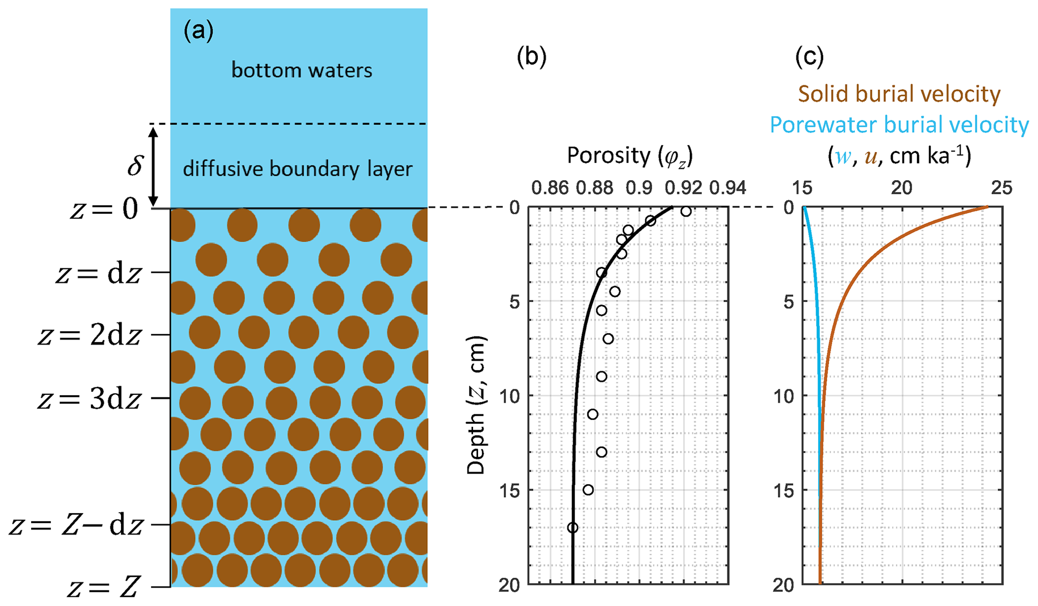
Figure 1 Schematic of RADI's vertical structure alongside steady-state depth profiles of porosity φ_z (see Eqs. 3 and 4), porewater (u, solid light blue line) and solid (w, solid brown line) burial velocities at in situ conditions taken at station 7 of Sayles et al. (2001). Burial velocity varies with depth due to porosity, as described in Sect. 2.3. The open circles in the porosity profile are porosity measurements from Sayles et al. (2001).

Multiple numerical models simulating early diagenesis have previously been published (Burdige and Gieskes, 1983; Rabouille and Gaillard, 1991; Boudreau, 1996b; Van Cappellen and Wang, 1996; Soetaert et al., 1996b; Archer et al., 2002; Munhoven, 2007, 2021; Couture et al., 2010; Yakushev et al., 2017; Hülse et al., 2018), each with its own assumptions and best area of application (Paraska et al., 2014). For instance, most existing models are limited to a steady state and are thus unable to predict the transient sediment response to time-dependent phenomena such as tides, seasonal change, ocean deoxygenation, or acidification. Moreover, most of these models do not take the presence of a DBL into account, even though diffusion through the DBL may control the overall rate of many biogeochemical reactions. Finally, as the landscape of computing software and programming languages evolves and improves computing efficiency and code accessibility, it is important to leverage emerging developments to implement new biogeochemical models. Here, we describe a new sediment porewater model built upon earlier work termed RADI, an acronym accounting for the main processes included in the model that control the vertical distribution of solutes and solids: chemical reactions, advection, molecular and bio-diffusion, and bio-irrigation. The novelty of RADI is that it combines degradation-driven organic matter CaCO₃ dissolution (Archer et al., 2002) with a diffusive boundary layer (Boudreau, 1996b) and integrates the state-of-the art parameterization of CaCO₃ dissolution kinetics in seawater (Dong et al., 2019; Naviaux et al., 2019a). RADI thus links mechanistic surface reaction modeling to global-scale biogeochemical models (Carroll et al., 2020). By integrating components (e.g., total alkalinity) rather than individual chemical species (e.g., carbonate and bicarbonate ions), RADI is easy to compare to observations. RADI is implemented in two popular scientific programming languages: Julia and MATLAB/GNU Octave. To our knowledge, this is the first diagenetic model implemented in Julia (https://julialang.org, last access: 28 January 2022), a high-level, high-performance, and cross-platform programming language that is free and open source (Bezanson et al., 2017). Here, we first describe the scientific background behind RADI and its implementations. Following this, we evaluate its performance in three selected locations and explore other potential applications, such as the influence of tides and seasonality on early diagenesis in the deep ocean.

2 Model description

In the following section, we describe how reactions, advection, diffusion, and irrigation are implemented in RADIv1. Model variables are italicized and their names as coded in the model are shown in monospaced font. Tables 1 and 2 include an inventory of model variables and parameters and a list of nomenclature for chemical species, respectively.

Table 1 Nomenclature of model parameters and variables.

Table 2 Nomenclature of modeled chemical species. All variables are concentrations, expressed in mol per cubic meter of solid for solid species and mol per cubic meter of water for solute species.

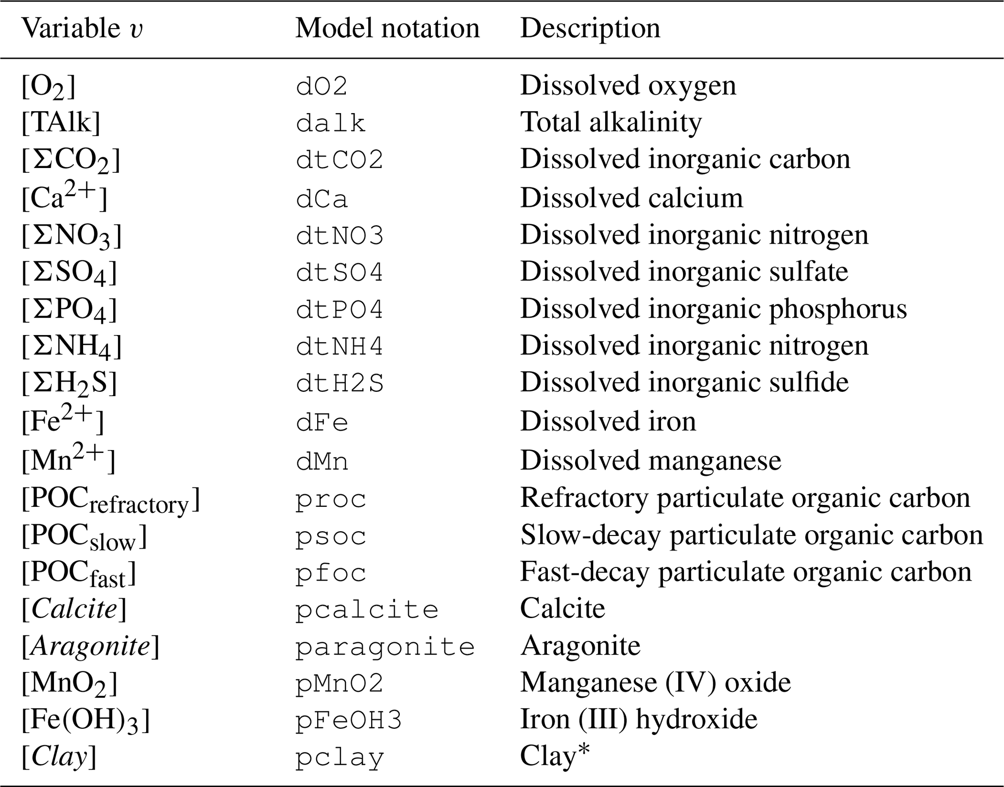
^* We consider all clay minerals to be montmorillonite (Al₂H₂O₁₂Si₄; molar mass is equal to 360.31 g mol⁻¹).

2.1 Model structure and fundamental equation

RADI uses the same set of reactive-transport partial differential equations as implemented in CANDI (Boudreau, 1996b), i.e., for each solute component,

$$\begin{array}{}\text{(1)}& {\displaystyle \frac{\partial \mathit{\nu }}{\partial t}}={\displaystyle \frac{\mathrm{1}}{\mathit{\phi }}}{\displaystyle \frac{\partial }{\partial z}}\left(\mathit{\phi }d{\displaystyle \frac{\partial \mathit{\nu }}{\partial z}}-\mathit{\phi }u\mathit{\nu }\right)+\mathit{\alpha }(v_{\mathrm{w}}-v)+\sum R,\end{array}$$

and for each solid component,

$$\begin{array}{}\text{(2)}& {\displaystyle \frac{\partial \mathit{\nu }}{\partial t}}={\displaystyle \frac{\mathrm{1}}{{\mathit{\phi }}_{\mathrm{s}}}}{\displaystyle \frac{\partial }{\partial z}}\left({\mathit{\phi }}_{\mathrm{s}}b{\displaystyle \frac{\partial \mathit{\nu }}{\partial z}}-{\mathit{\phi }}_{\mathrm{s}}w\mathit{\nu }\right)+\sum R,\end{array}$$

where v is the concentration of a given component, t is time, φ is sediment porosity, φ_s is the solid–volume fraction, d is the effective molecular diffusion coefficient, b is the bioturbation coefficient, z is depth, u is the porewater burial velocity, w is the solid burial velocity, α is the irrigation coefficient, v_w is the concentration of a solute in the bottom waters, and ΣR is the net production rate from all biogeochemical reactions for a given component. Each of these terms will be described in detail later in this section. These partial differential equations are solved numerically using the method of lines described in Boudreau (1996b). Instead of searching for steady-state solutions directly, RADI computes the concentrations of a set of solids and solutes at each depth and time step following a time vector set by the user. The user determines the simulation time depending on the objectives, e.g., multimillennial to predict a steady state, or a few days to study the response of the sedimentary system to high-frequency cyclic phenomena such as tides. For initial conditions, the user can choose between predefined uniform values (e.g., set all concentrations to zero) or a set of saved concentrations (e.g., from a previous simulation that has reached steady state). T is the total simulation time, dt is the temporal resolution, i.e., the interval between each time step, and t refers to the array of modeled time points. All time units are in years (a). The interface between the surface sediment and overlying seawater, conventionally set at a sediment depth z=0, represents the top layer of RADI's vertical axis (Fig. 1). The bottom layer of the model is at a sediment depth Z. Between these limits, n layers are present, each being separated by a constant vertical gap dz. Depth units are in meters. The values assigned to dz and dt depend on the nature of the problem and on the kinetics of the chemical reactions. In the present study, all cases use dz=2 mm and $\mathrm{d}t=\mathrm{1}/\mathrm{128}\mathrm{000}$ a, i.e., ∼4 min. If a lower dz is used, dt needs to be lowered as well to preserve numerical stability. In general, the ratio $\mathrm{d}z/\mathrm{d}t$ should be kept below a value of 256 m a⁻¹. If dz is divided by two, dt needs to be divided by two as well, and the speed at which RADI runs will be reduced by a factor of four.

RADI operates on a static, user-defined porosity profile. Sediment porosity, φ_z in Fig. 1, refers to the porewater volume fraction in the sediment (dimensionless) and typically decreases exponentially with sediment depth due to steady-state compaction. The sediment porosity profile is parameterized following Boudreau (1996b) as follows:

$$\begin{array}{}\text{(3)}& {\mathit{\phi }}_z={\mathit{\phi }}_{\mathrm{\infty }}+({\mathit{\phi }}_{\mathrm{0}}-{\mathit{\phi }}_{\mathrm{\infty }})e^{-\mathit{\beta }z},\end{array}$$

where φ_∞ is the porosity at great depth, φ₀ is the porosity at the sediment–water interface, and β is an attenuation coefficient (in m⁻¹). A typical deep-sea sediment porosity profile is shown in Fig. 1. Here the measured porosity profile at station 7 of cruise NBP98-2 (Sayles et al., 2001) is fit using φ_∞=0.87, φ₀=0.915, and β=33 m⁻¹. The solid volume fraction (φ_s, dimensionless) is defined as follows:

$$\begin{array}{}\text{(4)}& {\mathit{\phi }}_{\mathrm{s},z}=\mathrm{1}-{\mathit{\phi }}_z,\end{array}$$

and increases with sediment depth (as compaction forces squeeze porewaters out).

Within this grid and for each time step, RADI computes the concentrations of 11 solute variables (TAlk, ΣCO₂, O₂, Ca²⁺, ΣNO₃, ΣSO₄, ΣPO₄, ΣNH₄, ΣH₂S, Fe²⁺, and Mn²⁺) and 8 solid variables (Calcite, Aragonite, Fe(OH)₃, MnO₂, Clay, and three kinds of particulate organic carbon, collectively termed POC). Note that clay is simply modeled as a non-reactive solid that is included because the clay accumulation flux to the sediment–water interface participates in the calculation of the solid burial velocity; see Sect. 2.3. Concentration units are in mol per square meter of water for solutes and in mol per square meter of solid for solid species. For each modeled solute or solid concentration v at time t and sediment depth z, the following equation applies:

$$\begin{array}{}\text{(5)}& v_{(t+\mathrm{d}t),z}=v_{t,z}+\left[R\right(v_{t,z})+A(v_{t,z})+D(v_{t,z})+I(v_{t,z}\left)\right]\cdot \mathrm{d}t,\end{array}$$

where R(v_t,z) quantifies the rate of change of v_t,z due to chemical reactions, A(v_t,z) quantifies the rate of change of v_t,z due to advection, D(v_t,z) quantifies the rate of change of v_t,z due to molecular and bio-diffusion, and I(v_t,z) quantifies the rate of change of v_t,z due to bio-irrigation. In general, only the subscript z variables are explicitly written out in this paper for variables and parameters that vary with depth. The t variables are implicit but excluded for clarity.

2.2 Reactions

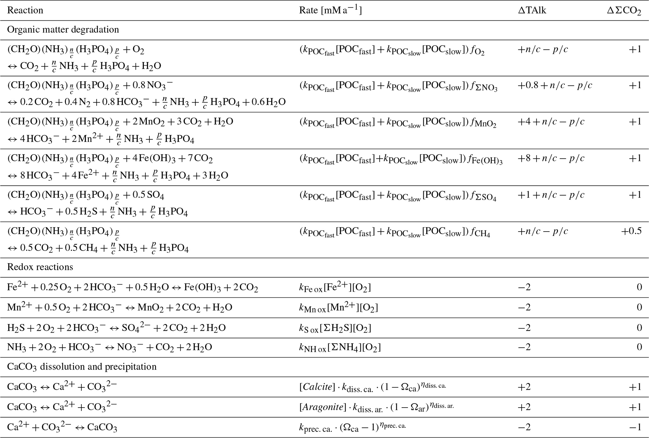
In RADI, biogeochemical reactions operate on solutes and solids throughout the entire sediment column, including the very top and bottom layers. R(v_z) is the net rate at which v_z is being consumed (negative R) or produced (positive R) by these reactions. Biogeochemical reactions in RADI (Table 3) are grouped into three categories: (i) organic matter degradation, (ii) oxidation of reduced metabolites (organic matter degradation byproducts), and (iii) dissolution or precipitation of calcium carbonate minerals. RADI has been designed for early diagenesis in deep-sea sediments, and thus formation and re-oxidation of metal sulfide minerals are not considered.

Table 3 Diagenetic reactions, reaction rates, and reaction contributions to porewater.

2.2.1 Organic matter degradation

Organic carbon deposited on the seafloor originates mainly from primary production in the upper ocean or on land and (to a lesser extent) from the ocean interior via chemoautotrophy. Despite the differences in origin, detrital organic matter found in marine sediments typically has the same composition: ∼60 % proteins, ∼20 % lipids, ∼20 % carbohydrates, and a fraction of other compounds (Hedges et al., 2002; Burdige, 2007; Middelburg, 2019). Here, the stoichiometry of organic matter is represented by the coefficients c (for carbon), n (for nitrogen), and p (for phosphorus). By default, the c:p ratio is set to 106:1 and the n:p ratio set to 16:1, following the Redfield ratio that describes the average composition of phytoplankton biomass (Redfield, 1958), but these values can easily be adjusted. In RADI, $c/p$ is denoted RC, $n/p$ is denoted RN, and $p/p$ is denoted RP, which is unity. Organic matter is also simplified here as an elementary carbohydrate (CH₂O). In reality, loss of H and O during biosynthesis of proteins, lipids, and polysaccharides occurs (Anderson, 1995; Hedges et al., 2002; Middelburg, 2019), which results in an effective molar ratio of O₂ consumed to C degraded of ∼1.2 during aerobic respiration (Anderson and Sarmiento, 1994) instead of 1 as assumed here (Table 3).

Observations show that some organic compounds are preferentially degraded and become selectively depleted (Cowie and Hedges, 1994; Lee et al., 2000). As a result, the bulk reactivity of organic matter decreases with increasing age (Middelburg, 1989). Degradation of organic matter deposited at the seafloor typically follows a sequential utilization of available oxidants, O₂, ${{\mathrm{NO}}_{\mathrm{3}}}^{-}$, MnO₂, Fe(OH)₃, and ${{\mathrm{SO}}_{\mathrm{4}}}^{\mathrm{2}-}$, followed by methanogenesis (Froelich et al., 1979; Berner, 1980; Arndt et al., 2013). All organic matter degradation reactions implemented in RADI are shown in Table 3.

To account for the decrease in organic matter degradation rate with sediment depth, we separate organic matter into fractions of different reactivity, and we assign a rate constant to each of the degradable fractions. Following Jørgensen (1978), Westrich and Berner (1984), and Soetaert et al. (1996b), three different classes of organic matter are considered: refractory, slow-decay, and fast-decay organic matter. The refractory organic matter class is not reactive during the timescales considered here. The fast- and slow-decay organic matter fractions each have a depth-dependent, oxidant-independent reactivity. The overall organic matter degradation rate decreases with depth because the quantity of organic matter and the relative proportions of fast- and slow-decay materials decline with depth. Organic matter is degraded following the sequential utilization of available oxidants. The oxidant limitation is represented by a Michaelis–Menten-type (also termed “Monod”) function, in which each oxidant has an associated half-saturation constant (K_oxidant in mol m⁻³) that symbolizes the oxidant concentration at which the process proceeds at half its maximal speed (Soetaert et al., 1996b). The presence of some oxidants may also inhibit other metabolic pathways; this is represented by an inhibition constant ($K_{\text{oxidant}}^{\prime }$ in mol m⁻³) that is specific to each oxidant. These limiting and inhibitory functions have been widely used (Boudreau, 1996b; Van Cappellen and Wang, 1996; Soetaert et al., 1996b; Couture et al., 2010), they allow a single equation to be used for each component across the entire model depth range, and they also permit some overlap between the different pathways, as observed in nature (Froelich et al., 1979). In RADI, the overall degradation of fast- or slow-decay organic carbon occurs at the following rate:

$$\begin{array}{}\text{(6)}& R_{{\text{POC}}_{\text{fast\hspace{0.17em}or\hspace{0.17em}slow}},z}=f_{\text{oxidant},z}\cdot k_{{\text{POC}}_{\text{fast\hspace{0.17em}or\hspace{0.17em}slow}}}\cdot [{\text{POC}}_{\text{fast\hspace{0.17em}or\hspace{0.17em}slow}}{]}_z\end{array}$$

where k_POC is the rate constant for the degradation of a given type of organic carbon (fast- or slow-decay types, expressed in a⁻¹), [POC_{fast or slow}] is the concentration of organic carbon (fast- or slow-decay) in sediments, and f_Ox. is the sum of the fractions of organic carbon degraded by each oxidant (dimensionless, always equal to one), given by

$$\begin{array}{ll}{\displaystyle }{f}_{\text{oxidant},z}=& {\displaystyle }{f}_{{\mathrm{O}}_{\mathrm{2}},z}+f_{\mathrm{\Sigma }{\mathrm{NO}}_{\mathrm{3}},z}+f_{{\mathrm{MnO}}_{\mathrm{2}},z}+f_{\mathrm{Fe}(\mathrm{OH}{)}_{\mathrm{3}},z}\\ \text{(7)}& {\displaystyle }& {\displaystyle }+f_{\mathrm{\Sigma }{\mathrm{SO}}_{\mathrm{4}},z}+f_{{\mathrm{CH}}_{\mathrm{4}},z},\end{array}$$

where

$$\begin{array}{ll}\text{(8a)}& {\displaystyle }{f}_{{\mathrm{O}}_{\mathrm{2}},z}=& {\displaystyle }{\displaystyle \frac{[{\mathrm{O}}_{\mathrm{2}}{]}_z}{K_{{\mathrm{O}}_{\mathrm{2}}}+[{\mathrm{O}}_{\mathrm{2}}{]}_z}},{\displaystyle }{f}_{\mathrm{\Sigma }{\mathrm{NO}}_{\mathrm{3}},z}=& {\displaystyle }{\displaystyle \frac{[\mathrm{\Sigma }{\mathrm{NO}}_{\mathrm{3}}{]}_z}{K_{\mathrm{\Sigma }{\mathrm{NO}}_{\mathrm{3}}}+[\mathrm{\Sigma }{\mathrm{NO}}_{\mathrm{3}}{]}_z}}\\ \text{(8b)}& {\displaystyle }& {\displaystyle }\times {\displaystyle \frac{K_{{\mathrm{O}}_{\mathrm{2}}}^{\prime }}{K_{{\mathrm{O}}_{\mathrm{2}}}^{\prime }+[{\mathrm{O}}_{\mathrm{2}}{]}_z}},{\displaystyle }{f}_{{\mathrm{MnO}}_{\mathrm{2}},z}=& {\displaystyle }{\displaystyle \frac{[{\mathrm{MnO}}_{\mathrm{2}}{]}_z}{K_{{\mathrm{MnO}}_{\mathrm{2}}}+[{\mathrm{MnO}}_{\mathrm{2}}{]}_z}}{\displaystyle \frac{K_{\mathrm{\Sigma }{\mathrm{NO}}_{\mathrm{3}}}^{\prime }}{K_{\mathrm{\Sigma }{\mathrm{NO}}_{\mathrm{3}}}^{\prime }+[\mathrm{\Sigma }{\mathrm{NO}}_{\mathrm{3}}{]}_z}}\\ \text{(8c)}& {\displaystyle }& {\displaystyle }\times {\displaystyle \frac{K_{{\mathrm{O}}_{\mathrm{2}}}^{\prime }}{K_{{\mathrm{O}}_{\mathrm{2}}}^{\prime }+[{\mathrm{O}}_{\mathrm{2}}{]}_z}},{\displaystyle }{f}_{\mathrm{Fe}(\mathrm{OH}{)}_{\mathrm{3}},z}=& {\displaystyle }{\displaystyle \frac{[\mathrm{Fe}(\mathrm{OH}{)}_{\mathrm{3}}{]}_z}{K_{\mathrm{Fe}(\mathrm{OH}{)}_{\mathrm{3}}}+[\mathrm{Fe}(\mathrm{OH}{)}_{\mathrm{3}}{]}_z}}{\displaystyle \frac{K_{{\mathrm{MnO}}_{\mathrm{2}}}^{\prime }}{K_{{\mathrm{MnO}}_{\mathrm{2}}}^{\prime }+[{\mathrm{MnO}}_{\mathrm{2}}{]}_z}}\\ \text{(8d)}& {\displaystyle }& {\displaystyle }\times {\displaystyle \frac{K_{\mathrm{\Sigma }{\mathrm{NO}}_{\mathrm{3}}}^{\prime }}{K_{\mathrm{\Sigma }{\mathrm{NO}}_{\mathrm{3}}}^{\prime }+[\mathrm{\Sigma }{\mathrm{NO}}_{\mathrm{3}}{]}_z}}{\displaystyle \frac{K_{{\mathrm{O}}_{\mathrm{2}}}^{\prime }}{K_{{\mathrm{O}}_{\mathrm{2}}}^{\prime }+[{\mathrm{O}}_{\mathrm{2}}{]}_z}},{\displaystyle }{f}_{\mathrm{\Sigma }{\mathrm{SO}}_{\mathrm{4}},z}=& {\displaystyle }{\displaystyle \frac{[\mathrm{\Sigma }{\mathrm{SO}}_{\mathrm{4}}{]}_z}{K_{\mathrm{\Sigma }{\mathrm{SO}}_{\mathrm{4}}}+[\mathrm{\Sigma }{\mathrm{SO}}_{\mathrm{4}}{]}_z}}{\displaystyle \frac{K_{\mathrm{Fe}(\mathrm{OH}{)}_{\mathrm{3}}}^{\prime }}{K_{\mathrm{Fe}(\mathrm{OH}{)}_{\mathrm{3}}}^{\prime }+[\mathrm{Fe}(\mathrm{OH}{)}_{\mathrm{3}}{]}_z}}\\ {\displaystyle }& {\displaystyle }\times {\displaystyle \frac{K_{{\mathrm{MnO}}_{\mathrm{2}}}^{\prime }}{K_{{\mathrm{MnO}}_{\mathrm{2}}}^{\prime }+[{\mathrm{MnO}}_{\mathrm{2}}{]}_z}}{\displaystyle \frac{K_{\mathrm{\Sigma }{\mathrm{NO}}_{\mathrm{3}}}^{\prime }}{K_{\mathrm{\Sigma }{\mathrm{NO}}_{\mathrm{3}}}^{\prime }+[\mathrm{\Sigma }{\mathrm{NO}}_{\mathrm{3}}{]}_z}}\\ \text{(8e)}& {\displaystyle }& {\displaystyle }\times {\displaystyle \frac{K_{{\mathrm{O}}_{\mathrm{2}}}^{\prime }}{K_{{\mathrm{O}}_{\mathrm{2}}}^{\prime }+[{\mathrm{O}}_{\mathrm{2}}{]}_z}},{\displaystyle }{f}_{{\mathrm{CH}}_{\mathrm{4}},z}=& {\displaystyle }{\displaystyle \frac{K_{\mathrm{\Sigma }{\mathrm{SO}}_{\mathrm{4}}}^{\prime }}{K_{\mathrm{\Sigma }{\mathrm{SO}}_{\mathrm{4}}}^{\prime }+[\mathrm{\Sigma }{\mathrm{SO}}_{\mathrm{4}}{]}_z}}{\displaystyle \frac{K_{\mathrm{Fe}(\mathrm{OH}{)}_{\mathrm{3}}}^{\prime }}{K_{\mathrm{Fe}(\mathrm{OH}{)}_{\mathrm{3}}}^{\prime }+[\mathrm{Fe}(\mathrm{OH}{)}_{\mathrm{3}}{]}_z}}\\ {\displaystyle }& {\displaystyle }\times {\displaystyle \frac{K_{{\mathrm{MnO}}_{\mathrm{2}}}^{\prime }}{K_{{\mathrm{MnO}}_{\mathrm{2}}}^{\prime }+[{\mathrm{MnO}}_{\mathrm{2}}{]}_z}}{\displaystyle \frac{K_{\mathrm{\Sigma }{\mathrm{NO}}_{\mathrm{3}}}^{\prime }}{K_{\mathrm{\Sigma }{\mathrm{NO}}_{\mathrm{3}}}^{\prime }+[\mathrm{\Sigma }{\mathrm{NO}}_{\mathrm{3}}{]}_z}}\\ \text{(8f)}& {\displaystyle }& {\displaystyle }\times {\displaystyle \frac{K_{{\mathrm{O}}_{\mathrm{2}}}^{\prime }}{K_{{\mathrm{O}}_{\mathrm{2}}}^{\prime }+[{\mathrm{O}}_{\mathrm{2}}{]}_z}}.\end{array}$$

Half-saturation and inhibition constants for each oxidant used in RADI are given in Table 4. The degradation rate constant of organic carbon, $k_{{\text{POC}}_{\text{fast\hspace{0.17em}or\hspace{0.17em}slow}}}$, is computed as a function of the flux of organic carbon reaching the seafloor and is sediment depth dependent (Archer et al., 2002):

$$\begin{array}{}\text{(9a)}& {\displaystyle }{k}_{{\text{POC}}_{\text{fast}}}& {\displaystyle }=(\mathrm{1.5}\times {\mathrm{10}}^{-\mathrm{1}})(F_{\text{POC}}\cdot {\mathrm{10}}^{\mathrm{2}}{)}^{\mathrm{0.85}},\text{(9b)}& {\displaystyle }{k}_{{\text{POC}}_{\text{slow}}}& {\displaystyle }=(\mathrm{1.3}\times {\mathrm{10}}^{-\mathrm{4}})(F_{\text{POC}}\cdot {\mathrm{10}}^{\mathrm{2}}{)}^{\mathrm{0.85}},\end{array}$$

where F_POC is the total flux of organic carbon reaching the seafloor (i.e., fast, slow, and refractory, in $\mathrm{mol}{\mathrm{m}}^{-\mathrm{2}}{\mathrm{a}}^{-\mathrm{1}}$). The numbers $\mathrm{1.3}\times {\mathrm{10}}^{-\mathrm{4}}$ and $\mathrm{1.5}\times {\mathrm{10}}^{-\mathrm{1}}$ have been tuned to best fit observations of both a Southern Ocean station and a North Atlantic station; see Sect. 3.

Table 4 Suggested values for model parameters.

¹ Assuming a solid density of 2.65 g cm⁻³. ² Values for the “deep sea”.

2.2.2 Oxidation of organic matter degradation by-products

Organic matter degradation reactions primarily change oxidants (e.g., O₂, ${{\mathrm{NO}}_{\mathrm{3}}}^{-}$, MnO₂, Fe(OH)₃, ${{\mathrm{SO}}_{\mathrm{4}}}^{\mathrm{2}-}$) into their reduced forms (e.g., H₂O, N₂, Mn²⁺, Fe²⁺, H₂S; Table 3). If oxygen is introduced into the system or the reduced metabolites diffuse upwards in oxic porewaters, then these reduced byproducts are converted back into their oxidized form and the energy contained in them becomes available to the microbial community, though these energetics are not considered in RADI.

Here, four redox reactions involving organic matter degradation byproducts are implemented (Table 3): oxidation of Fe²⁺, Mn²⁺, ΣH₂S, and ΣNH₃, respectively. These four reactions consume porewater total alkalinity (TAlk) but do not alter porewater ΣCO₂ (Table 3), thus locally acidifying porewaters. Here, we use the TAlk definition of Dickson (1981), in which TAlk is defined as “the number of moles of hydrogen ion equivalent to the excess of proton acceptors (bases formed from weak acids with a dissociation constant $K\le {\mathrm{10}}^{-\mathrm{4.5}}$ and zero ionic strength) over proton donors (acids with $K>{\mathrm{10}}^{-\mathrm{4.5}}$) in one kilogram of sample.” This scheme should be sufficient for all open-ocean applications but may not be suitable for coastal and anoxic environments with extensive metal sulfide mineral turnover, which require a more complete set of redox reactions such as that from the CANDI model of Boudreau (1996b). Additional components and reactions can easily be implemented in future versions (see Sect. 5). The rate constants for these four redox reactions are taken from Boudreau (1996b) and reported in Table 4.

2.2.3 CaCO₃ dissolution and precipitation

RADI includes two CaCO₃ polymorphs: low Mg calcite and aragonite, but more could be added in future versions, e.g., high Mg calcite and/or vaterite. Calcite and aragonite both have different dissolution kinetics, in which their dissolution rates increase as the undersaturation state of seawater with respect to calcite ($\mathrm{1}-{\mathrm{\Omega }}_{\text{ca},z}$) or aragonite ($\mathrm{1}-{\mathrm{\Omega }}_{\text{ar},z}$) increases (Keir, 1980; Walter and Morse, 1985; Sulpis et al., 2017; Dong et al., 2019; Naviaux et al., 2019b). Here, Ω_z is the sediment-depth-dependent saturation state of seawater with respect to calcite or aragonite, computed as $[{\mathrm{Ca}}^{\mathrm{2}+}{]}_z\cdot [{{\mathrm{CO}}_{\mathrm{3}}}^{\mathrm{2}-}{]}_z/K_{\text{sp}}^{\ast }$, where $K_{\text{sp}}^{\ast }$ is the stoichiometric solubility constant of calcite or aragonite at in situ temperature, pressure, and salinity, as given in Mucci (1983) and Millero (1995). At each time step, Ω_z is computed using porewater [Ca²⁺]_z and $[{{\mathrm{CO}}_{\mathrm{3}}}^{\mathrm{2}-}{]}_z$ from the previous time step, the latter being calculated as a function of TAlk and the proton concentration [H⁺]. At each model time step, the total hydrogen ion concentration [H⁺] is computed from TAlk and ∑CO₂ using a single Newton–Raphson iteration from the previous time step (Humphreys et al., 2022):

$$\begin{array}{ll}{\displaystyle }[{\mathrm{H}}^{+}{]}_t& {\displaystyle }=[{\mathrm{H}}^{+}{]}_{t-\mathrm{1}}\\ \text{(10)}& {\displaystyle }& {\displaystyle }-{\displaystyle \frac{\left[\text{TAlk}\right]\left(\right[{\mathrm{H}}^{+}{]}_{t-\mathrm{1}},[\sum {\mathrm{CO}}_{\mathrm{2}}])-[\text{TAlk}]}{\mathrm{d}\left[\text{TAlk}\right]\left(\right[{\mathrm{H}}^{+}{]}_{t-\mathrm{1}},[\sum {\mathrm{CO}}_{\mathrm{2}}])/\mathrm{d}[{\mathrm{H}}^{+}{]}_{t-\mathrm{1}}}},\end{array}$$

where [H⁺]_t is the new [H⁺] value and $[{\mathrm{H}}^{+}{]}_{t-\mathrm{1}}$ is the [H⁺] from the previous time step. TAlk($[{\mathrm{H}}^{+}{]}_{t-\mathrm{1}}$, ∑CO₂) is the total alkalinity computed from user-specified total dissolved silicate, [∑PO₄] and total borate calculated from salinity (Uppström, 1974), plus equilibrium constants for silicic acid (Sillén et al., 1964) and phosphoric acid (Yao and Millero, 1995). Its derivative is computed following the approach of CO2SYS; see Humphreys et al. (2022). The carbonate ion concentration is then computed as follows:

$$\begin{array}{}\text{(11)}& \left[{{\mathrm{CO}}_{\mathrm{3}}}^{\mathrm{2}-}\right]={\displaystyle \frac{[\sum {\mathrm{CO}}_{\mathrm{2}}]\times K_{\mathrm{1}}^{\ast }\times K_{\mathrm{2}}^{\ast }}{K_{\mathrm{1}}^{\ast }\times K_{\mathrm{2}}^{\ast }+K_{\mathrm{1}}^{\ast }\times [{\mathrm{H}}^{+}{]}_t+[{\mathrm{H}}^{+}{]}_t^{\mathrm{2}}}},\end{array}$$

where $K_{\mathrm{1}}^{\ast }$ and $K_{\mathrm{2}}^{\ast }$ are the first and second dissociation constants for carbonic acid, respectively, taken from Lueker et al. (2000).

The dissolution rates (R_diss, in $\mathrm{mol}{\mathrm{m}}^{-\mathrm{3}}{\mathrm{a}}^{-\mathrm{1}}$) of calcite (solid blue line in Fig. 2a) and of aragonite (solid red line in Fig. 2a) as a function of (1−Ω_ca) are empirically defined as follows:

$$\begin{array}{}\text{(12)}& {\displaystyle }{R}_{\text{diss.\hspace{0.17em}ca.},z}& {\displaystyle }=\left[\mathit{\text{Calcite}}\right]\cdot k_{\text{diss.\hspace{0.17em}ca.}}\cdot (\mathrm{1}-{\mathrm{\Omega }}_{\text{ca}}{)}^{\mathit{\eta }\text{diss.\hspace{0.17em}ca.}},\text{(13)}& {\displaystyle }{R}_{\text{diss.\hspace{0.17em}ar.},z}& {\displaystyle }=\left[\mathit{\text{Aragonite}}\right]\cdot k_{\text{diss.\hspace{0.17em}ar.}}\cdot (\mathrm{1}-{\mathrm{\Omega }}_{\text{ar}}{)}^{{\mathit{\eta }}_{\text{diss.\hspace{0.17em}ar.}}}.\end{array}$$

In these expressions, the dissolution rate constant (k_diss, in a⁻¹) and the reaction order (η_diss, unitless) are mineral specific. The dissolution rate constants implicitly account for each mineral's specific surface area. Similar formulations have previously been implemented to describe calcite dissolution rates (e.g., Archer et al., 2002) but in most cases used a high reaction order and a tuned rate constant independent of solution chemistry (Fig. 2). Such discretizations are convenient but lack a mechanistic description of the controls on calcite dissolution in seawater (Adkins et al., 2021).

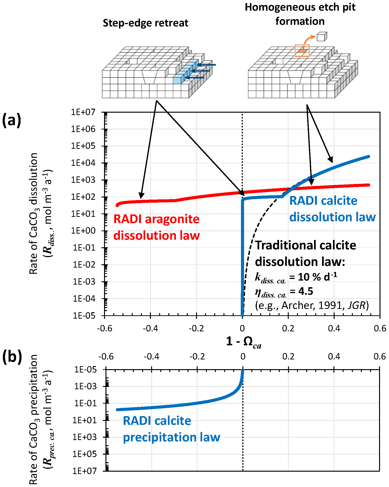
Figure 2 (a) Dissolution rate of calcite as computed using Eq. (12) and [Calcite]=10⁴ mol m⁻³ (solid blue line), and dissolution rate of aragonite as computed using Eq. (13) and [Aragonite]=10⁴ mol m⁻³ (solid red line). Note that for each dissolution rate profile, two different rate constants (k_diss) and reaction orders (η_diss) are used, depending on the seawater saturation state, with each accounting for a separate dissolution mechanism, i.e., step-edge retreat or homogeneous-edge pit formation. The dashed black line stands for a “traditional” dissolution rate profile obtained using [Calcite]=10⁴ mol m⁻³, a single dissolution rate constant for the entire (1−Ω_ca) range k_diss=10 % d⁻¹, and a reaction order η_diss of 4.5. (b) Precipitation rate of calcite as computed from Eq. (14). Note that dissolution rates are normalized here per total solid sediment volume and not per CaCO₃ surface area as in traditional kinetics studies.

The latest advances using isotope-labeling approaches to study carbonate dissolution kinetics show abrupt changes in dissolution mechanism depending on solution saturation state with either calcite or aragonite (Subhas et al., 2017; Dong et al., 2019; Naviaux et al., 2019a, b). Close to equilibrium, dissolution occurs primarily at sites on the crystal surfaces that are most exposed to the solution, e.g., steps and kinks. Further away from equilibrium, dissolution etch pits are activated at surface sites associated with defects and impurity atoms. Far away from equilibrium, there is enough free energy for dissolution etch pits to occur anywhere on the mineral surface, without the aid of crystal defects (Adkins et al., 2021). However, at temperatures most relevant to the deep oceans, ∼5 ^∘C or less, the defect-assisted dissolution mechanism is skipped (Naviaux et al., 2019b) and only the step-edge retreat (close to equilibrium) and homogeneous etch-pit formation (far away from equilibrium) dissolution regimes remain (Naviaux et al., 2019b) (Fig. 2). For both aragonite and calcite, while homogeneous etch-pit formation is indeed associated with a high-order dependency on the solution saturation state, step-edge retreat dissolution rates dominating near equilibrium show very little dependence on seawater saturation (Dong et al., 2019; Naviaux et al., 2019a). This could have significant consequences for the predicted carbonate dissolution rate near equilibrium: saturation-state-independent step-edge retreat dissolution will always be predicted to be faster close to equilibrium than dissolution associated with a high reaction order because a high reaction order forces the dissolution rate to converge to zero as the solution gets closer to equilibrium (Fig. 2).

Naviaux et al. (2019a) derived reaction orders for two separate regions of the (1−Ω_ca) spectrum: the Ω_ca threshold value dividing these two regions was Ω_{ca. critical}≈0.8. Here, based on the results of Naviaux et al. (2019a), we set η_diss. ca.=0.11 for $\mathrm{0.828}<{\mathrm{\Omega }}_{\text{ca}}<\mathrm{1}$ and η_diss. ca.=4.7 for Ω_ca≤0.828. The Ω_{ca critical} value used here is slightly higher than the ∼0.8 value given in Naviaux et al. (2019a) in order to have a smooth transition between defect-assisted and homogeneous dissolution. For aragonite, based on the results of Dong et al. (2019), we set η_diss. ar.=0.13 for $\mathrm{0.835}<{\mathrm{\Omega }}_{\text{ar}}<\mathrm{1}$ and η_diss. ar.=1.46 for Ω_ar≤0.835. The rate constants are tuned to best fit the observations in the two stations presented in Sect. 3. We use $k_{\text{diss.\hspace{0.17em}ca.}}=\mathrm{6.3}\times {\mathrm{10}}^{-\mathrm{3}}$ a⁻¹ for $\mathrm{0.828}<{\mathrm{\Omega }}_{\text{ca}}<\mathrm{1}$, k_diss. ca.=20 a⁻¹ for Ω_ca≤0.828, $k_{\text{diss.\hspace{0.17em}ar.}}=\mathrm{3.8}\times {\mathrm{10}}^{-\mathrm{3}}$ a⁻¹ for $\mathrm{0.835}<{\mathrm{\Omega }}_{\text{ar}}<\mathrm{1}$, and $k_{\text{diss.\hspace{0.17em}ar.}}=\mathrm{4.2}\times {\mathrm{10}}^{-\mathrm{2}}$ a⁻¹ for Ω_ar≤0.835. Both calcite and aragonite dissolution rate constants are lower than the values reported in the original publications. We suspect that (i) the reactive surface area of grains in sediments is much smaller than their specific surface area measured using adsorption isotherms via the Brunauer–Emmett–Teller (BET) method and (ii) unaccounted dissolution inhibitors are present in sediments, such as dissolved organic carbon (Naviaux et al., 2019a). A comparison of the steady-state [${{\mathrm{CO}}_{\mathrm{3}}}^{\mathrm{2}-}$] and [Calcite] porewater profiles predicted by RADI using the tuned rate constants implemented in RADIv1 and the original rate constants is shown in Fig. S1 in the Supplement.

Calcite precipitation is also included in the model and its rate (solid blue line in Fig. 2b) is parameterized with the following function:

$$\begin{array}{}\text{(14)}& R_{\text{prec.\hspace{0.17em}ca.},z}=k_{\text{prec.\hspace{0.17em}ca.}}\cdot ({\mathrm{\Omega }}_{\text{ca}}-\mathrm{1}{)}^{{\mathit{\eta }}_{\text{prec.\hspace{0.17em}ca.}}},\end{array}$$

where k_prec. ca is the precipitation rate constant set to 0.4 $\mathrm{mol}{\mathrm{m}}^{-\mathrm{3}}{\mathrm{a}}^{-\mathrm{1}}$ and η is equal to 1.76. The precipitation reaction order is taken from Zuddas and Mucci (1998), corrected for a seawater-like ionic strength of 0.7 mol kg⁻¹. The precipitation and dissolution rate continuum implemented in RADI (see Fig. 2) is very different from what a classic model with only calcite dissolution following high reaction order kinetics would display. For comparison, the dissolution rate of calcite using a dissolution rate constant k_diss of 10 % d⁻¹ and a reaction order η of 4.5, as implemented in most diagenetic models, including Archer (1991), is shown in Fig. 2a. The value of 10 % d⁻¹ for the rate constant was chosen because it makes the “traditional” calcite dissolution law overlap with the RADI dissolution law so that any differences between the two can be attributed to enhanced dissolution caused by step-edge retreat close to equilibrium. Mechanistic interpretations of the “kinks” in the dissolution rate profiles and of a non-zero dissolution rate near equilibrium still require more research, but the implications of these features for our understanding of marine CaCO₃ cycles can be explored with the present model.

2.3 Advection

The solid burial velocity at the sediment–water interface, w₀ in m a⁻¹, is given by

$$\begin{array}{}\text{(15)}& w_{\mathrm{0}}=\sum {\displaystyle \frac{F_v\cdot M_v}{{\mathit{\rho }}_v}}/{\mathit{\phi }}_{\mathrm{s},\mathrm{0}},\end{array}$$

where F_v is the flux of a solid species at the sediment–water interface ($\mathrm{mol}{\mathrm{m}}^{-\mathrm{2}}{\mathrm{a}}^{-\mathrm{1}}$), M_v is the molar mass of that solid (g mol⁻¹), and ρ_v is its solid density (g m⁻³). The solid and porewater burial velocity at greater depth are assumed to be equal and are computed as follows:

$$\begin{array}{}\text{(16)}& w_{\mathrm{\infty }}=u_{\mathrm{\infty }}=w_{\mathrm{0}}{\mathit{\phi }}_{\mathrm{s},\mathrm{0}}/{\mathit{\phi }}_{\mathrm{s},\mathrm{\infty }}.\end{array}$$

Thus, the porewater burial velocity, u, at all depths is

$$\begin{array}{}\text{(17)}& u_z=u_{\mathrm{\infty }}{\mathit{\phi }}_{\mathrm{\infty }}/{\mathit{\phi }}_z,\end{array}$$

and the solid burial velocity, w, is

$$\begin{array}{}\text{(18)}& w_z=w_{\mathrm{\infty }}{\mathit{\phi }}_{\mathrm{s},\mathrm{\infty }}/{\mathit{\phi }}_{\mathrm{s},z}.\end{array}$$

Depth profiles of u and w are shown in Fig. 1, computed from the solid fluxes at station 7 of cruise NBP98-2 (Sayles et al., 2001); see Sect. 3.2. In Fig. 1, the sharp porosity decline in the top centimeters of the sediments causes the solid fraction at ∼5 cm depth to be roughly 50 % higher than just below the interface. This leads to a solid burial velocity decrease of about the same magnitude (Fig. 1).

Advection is implemented following Boudreau (1996b), where the advection rate (A_z, in $\mathrm{mol}{\mathrm{m}}^{-\mathrm{3}}{\mathrm{a}}^{-\mathrm{1}}$) for solutes is given by

$$\begin{array}{ll}{\displaystyle }{A}_z\left(v\right)=& {\displaystyle }-\left(u_z-{\displaystyle \frac{d_z\left(v\right)}{{\mathit{\phi }}_z}}\cdot {\displaystyle \frac{\mathrm{d}{\mathit{\phi }}_z}{\mathrm{d}z}}-d{}^{\circ }\left(v\right)\cdot {\displaystyle \frac{\mathrm{d}(\mathrm{1}/{\mathit{\theta }}_z^{\mathrm{2}})}{\mathrm{d}z}}\right)\\ \text{(19)}& {\displaystyle }& {\displaystyle }\cdot {\displaystyle \frac{v_{(z+\mathrm{d}z})-v_{(z-\mathrm{d}z})}{\mathrm{2}\mathrm{d}z}},\end{array}$$

where d_z is the effective diffusion coefficient for a given solute at a given depth (in m² a⁻¹), d^∘ is the “free-solution” molecular diffusion coefficient for a given solute (in m² a⁻¹), and θ_z is the depth-dependent tortuosity (unitless) defined in Sect. 2.4. For solids, a more sophisticated weighted-difference scheme is employed (Fiadeiro and Veronis, 1977; Boudreau, 1996b):

$$\begin{array}{ll}{\displaystyle }{A}_z\left(v\right)=& {\displaystyle }-\left(w_z-{\displaystyle \frac{\mathrm{d}{b}_z}{\mathrm{d}z}}-{\displaystyle \frac{b_z}{{\mathit{\phi }}_{\mathrm{s},z}}}\cdot {\displaystyle \frac{\mathrm{d}{\mathit{\phi }}_{\mathrm{s},z}}{\mathrm{d}z}}\right)\\ \text{(20)}& {\displaystyle }& {\displaystyle }\cdot {\displaystyle \frac{(\mathrm{1}-{\mathit{\sigma }}_z)v_{(z+\mathrm{d}z)}+\mathrm{2}{\mathit{\sigma }}_z{v}_z-(\mathrm{1}+{\mathit{\sigma }}_z)v_{(z-\mathrm{d}z)}}{\mathrm{2}\mathrm{d}z}},\end{array}$$

where b_z is the depth-dependent bioturbation coefficient (m² a⁻¹) and

$$\begin{array}{}\text{(21)}& {\mathit{\sigma }}_z\left(v\right)=\mathrm{1}/\tanh \left({\mathit{\text{Pe}}}_{h,z}\right)-\mathrm{1}/{\mathit{\text{Pe}}}_{h,z},\end{array}$$

where

$$\begin{array}{}\text{(22)}& {\mathit{\text{Pe}}}_{h,z}=w_z\cdot \mathrm{d}z/\mathrm{2}{b}_z.\end{array}$$

The parameter Pe_h is half of the cell Péclet number, which expresses the influence of advection relative to bioturbation across a distance separating two points of the grid, centered at the depth z. If bioturbation dominates (Pe_h≪1), e.g., near the sediment–water interface, σ_z tends toward zero and a centered-difference discretization is implemented. If advection dominates (Pe_h≫1), e.g., deeper in sediments, σ_z tends toward unity and backward-difference discretization prevails; see Eq. (20). This differencing scheme, originally developed by Fiadeiro and Veronis (1977), maintains stability in the entire sediment column (Boudreau, 1996b).

2.4 Diffusion

The diffusion flux of any species depends on its effective diffusion coefficient, d_z(v), which varies with depth within the sediment.

For each solute, free-solution diffusion coefficients, denoted d_z^∘(v), were computed at in situ temperatures (Li and Gregory, 1974; Boudreau, 1997; Schulz, 2006). For solute variables representing several individual species (e.g., ΣPO₄, ΣCO₂), the diffusion coefficient of the dominant species was considered. Given the high proportion of ${{\mathrm{HCO}}_{\mathrm{3}}}^{-}$ relative to ${{\mathrm{CO}}_{\mathrm{3}}}^{\mathrm{2}-}$ and CO_2 (aq) in seawater and porewaters (see Fig. S2 in the Supplement), the diffusion coefficient of ${{\mathrm{HCO}}_{\mathrm{3}}}^{-}$ was adopted for both TAlk and ΣCO₂. However, this approach may not be suited for sedimentary environments in which pH is lower than 7 because a greater proportion of dissolved inorganic species would then be under the form of carbonic acid, i.e., CO_2 (aq), which has a higher diffusion coefficient than ${{\mathrm{HCO}}_{\mathrm{3}}}^{-}$ (Fig. S2). Free-solution diffusion coefficients, their temperature dependencies, and their sources are reported in Table 5. The diffusion of solutes in the porewaters is slower than in an equivalent volume of water as a result of the physical barriers caused by the presence of solid grains in a sediment. To correct for this effect, we follow Boudreau (1996b) and compute the effective diffusion coefficient for a given solute as follows:

$$\begin{array}{}\text{(23)}& d_z\left(v\right)=d{}^{\circ }\left(v\right)/\left({\mathit{\theta }}_z^{\mathrm{2}}\right),\end{array}$$

where so-called tortuosity (θ) is defined as follows (Boudreau, 1996a):

$$\begin{array}{}\text{(24)}& {\mathit{\theta }}_z=\sqrt{\mathrm{1}-\mathrm{2}\ln \left({\mathit{\phi }}_z\right)}.\end{array}$$

Table 5 Temperature-dependent molecular diffusion coefficients (m² a⁻¹).

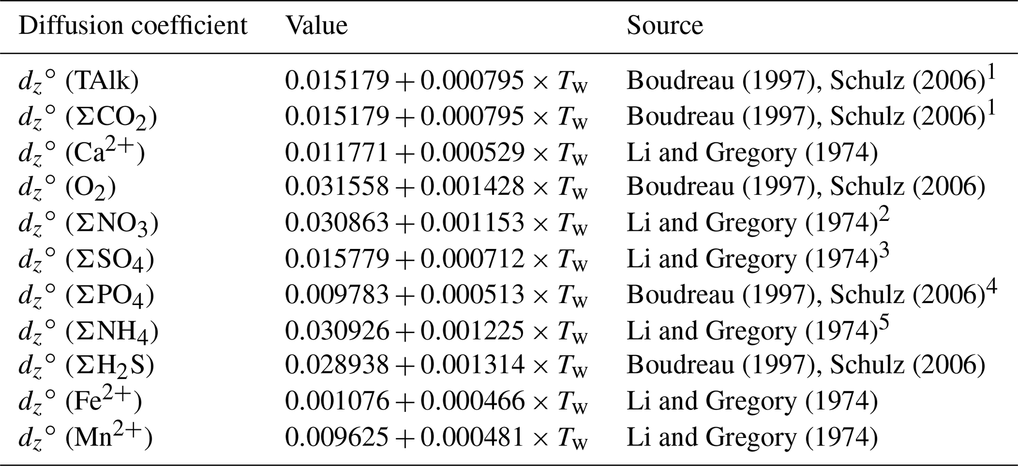
¹ value for ${{\mathrm{HCO}}_{\mathrm{3}}}^{-}$ ion, ² Value for ${{\mathrm{NO}}_{\mathrm{3}}}^{-}$ ion. ³ Value for ${{\mathrm{SO}}_{\mathrm{4}}}^{\mathrm{2}-}$ ion. ⁴ Value for ${{\mathrm{HPO}}_{\mathrm{4}}}^{\mathrm{2}-}$ ion. ⁵ Value for ${{\mathrm{NH}}_{\mathrm{4}}}^{+}$ ion.

For each solid, effective diffusion occurs through the mixing action of burrowing microorganisms, quantified using a bioturbation coefficient that decreases with depth. Archer et al. (2002) used a dataset including 53 sediment sites ranging in depth from 47 to 5668 m to derive an optimal bioturbation rate profile, in which the rate of bioturbation increases with increasing flux of total organic carbon reaching the seafloor (F_POC) and attenuates in low-oxygen conditions. This pattern was also observed by Smith et al. (1997) and Smith and Rabouille (2002). As in Archer et al. (2002), we couple both bioturbation and irrigation to the incoming carbon deposition flux (Fig. 3) rather than water depth or sediment accumulation rate (Boudreau, 1994; Middelburg et al., 1997; Soetaert et al., 1996c), although all these quantities are related to each other. From an ecological perspective, more carbon to the seafloor represents more food available to benthic communities, hence more biological transport. Linking bioturbation activity to carbon deposition flux also allows for a direct coupling with Earth system models simulating carbon sinking fluxes in the ocean. Following Archer et al. (2002), we express the surficial bioturbation mixing rate (b₀, in m² a⁻¹) as follows:

$$\begin{array}{}\text{(25)}& b_{\mathrm{0}}=(\mathrm{2.32}\times {\mathrm{10}}^{-\mathrm{6}})(F_{\text{POC}}\times {\mathrm{10}}^{\mathrm{2}}{)}^{\mathrm{0.85}},\end{array}$$

where F_POC is expressed in $\mathrm{mol}{\mathrm{m}}^{-\mathrm{2}}{\mathrm{a}}^{-\mathrm{1}}$. The bioturbation mixing rate at all depths (b_z, in m² a⁻¹) is

$$\begin{array}{}\text{(26)}& b_z=b_{\mathrm{0}}{e}^{-(z/{\mathit{\lambda }}_{\mathrm{b}}{)}^{\mathrm{2}}}{\displaystyle \frac{[{\mathrm{O}}_{\mathrm{2}}{]}_{\mathrm{w}}}{[{\mathrm{O}}_{\mathrm{2}}{]}_{\mathrm{w}}+\mathrm{0.02}}},\end{array}$$

where the characteristic depth λ_b=8 cm, following Archer et al. (2002), and [O₂]_w is the oxygen concentration in the bottom waters. This depth-dependent bioturbation mixing rate is common to all solids, and its depth distribution is shown in Fig. 3 as a function of in situ [O₂]_w and F_POC. The effective diffusion coefficient for solids is then set as follows:

$$\begin{array}{}\text{(27)}& d_z\left(v\right)=b_z.\end{array}$$

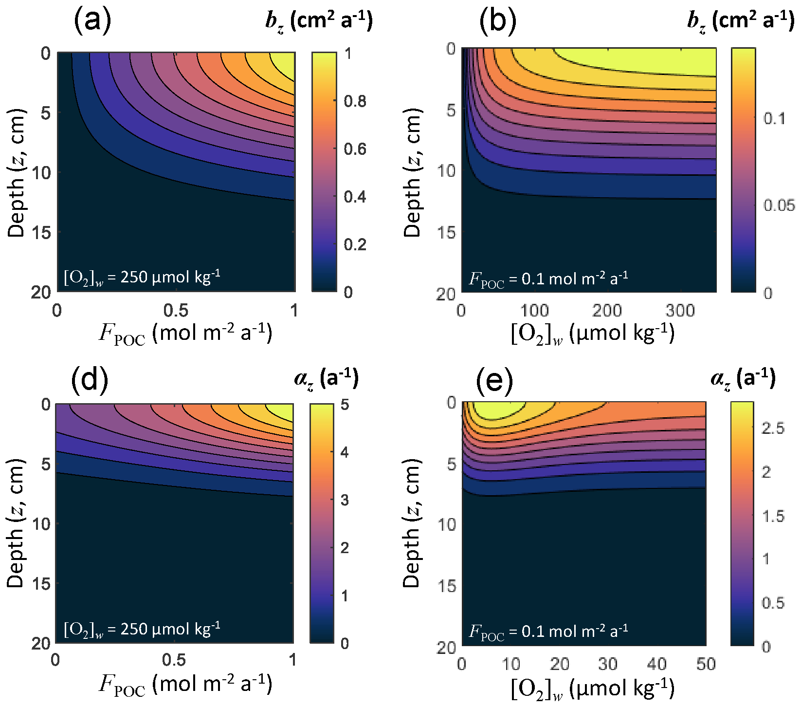
Figure 3 Bioturbation mixing rate b_z and irrigation coefficients α_z as a function of sediment depth z, organic carbon deposition flux F_POC, and dissolved oxygen concentration in the bottom waters [O₂]_w.

The (bio)diffusion is implemented in RADI following the centered difference discretization scheme from Boudreau (1996b). At sediment depth z, where $\mathrm{0}<z<Z$, for both solutes and solids:

$$\begin{array}{}\text{(28)}& D_z\left(v\right)=d_z\left(v\right)\cdot (v_{(z-\mathrm{d}z)}-\mathrm{2}{v}_z+v_{(z+\mathrm{d}z)})/(\mathrm{d}z{)}^{\mathrm{2}},\end{array}$$

where d_z(v) is the relevant effective diffusion coefficient.

2.5 Irrigation

The mixing of solutes caused by burrow flushing or ventilation occurs through an ensemble of processes collectively termed irrigation. Macroscopic burrows are often present in the seafloor sediment, with a complex three-dimensional structure and filled with oxygenated water that is ventilated for aerobic respiration. In a one-dimensional framework, this causes apparent internal sources or sinks of porewater solutes at particular depths (Boudreau, 1984; Emerson et al., 1984; Aller, 2001). Mathematically, this is parameterized as a non-local exchange function, i.e., a first-order kinetic reaction:

$$\begin{array}{}\text{(29)}& I_{t,z}\left(v\right)={\mathit{\alpha }}_z(v_{\mathrm{w}}-v_z),\end{array}$$

where α_z is an irrigation coefficient common to all solutes (expressed in a⁻¹). Following Archer et al. (2002), who used a dataset of 53 sediment sites comprised of microelectrode oxygen profiles and chamber oxygen fluxes across the sediment–water interface to derive an irrigation rate profile, we express the surficial irrigation coefficient as a function of the organic carbon deposition flux and the oxygen concentration of the overlaying waters:

$$\begin{array}{ll}{\displaystyle }{\mathit{\alpha }}_{\mathrm{0}}=& {\displaystyle }\mathrm{11}\left({\displaystyle \frac{{\tan }^{-\mathrm{1}}\left(\frac{\mathrm{5}{F}_{\text{POC}}\times {\mathrm{10}}^{\mathrm{2}}-\mathrm{400}}{\mathrm{400}}\right)}{\mathit{\pi }}}+\mathrm{0.5}\right)-\mathrm{0.9}\\ \text{(30)}& {\displaystyle }& {\displaystyle }+{\displaystyle \frac{\mathrm{20}[{\mathrm{O}}_{\mathrm{2}}{]}_{\mathrm{w}}}{[{\mathrm{O}}_{\mathrm{2}}{]}_{\mathrm{w}}+\mathrm{0.01}}}\cdot {\displaystyle \frac{F_{\text{POC}}\times {\mathrm{10}}^{\mathrm{2}}}{F_{\text{POC}}\times {\mathrm{10}}^{\mathrm{2}}+\mathrm{30}}}\cdot e^{\frac{-[{\mathrm{O}}_{\mathrm{2}}{]}_{\mathrm{w}}}{\mathrm{0.01}}}\end{array}$$

and the irrigation coefficient at all depths as follows:

$$\begin{array}{}\text{(31)}& {\mathit{\alpha }}_z={\mathit{\alpha }}_{\mathrm{0}}{e}^{-(z/{\mathit{\lambda }}_{\mathrm{i}}{)}^{\mathrm{2}}},\end{array}$$

where the characteristic depth λ_i is 5 cm (Archer et al., 2002). The depth distribution of the irrigation coefficient is shown in Fig. 3 as a function of in situ [O₂]_w and F_POC.

2.6 Boundary conditions

Modeling of advection and diffusion processes requires appropriate boundary conditions in the layers above and below (z−dz and z+dz, respectively). Effective values of each variable immediately adjacent to the modeled depth domain are calculated following Boudreau (1996b) and used to compute the effects of advection and diffusion in the top and bottom layers using the same equations as within the sediment itself.

At the sediment–water interface, RADI enables prescribed solid fluxes and a diffusive boundary layer control for solutes. Following Boudreau (1996b), we calculate advection and diffusion at z=0 for solutes and solids as follows:

$$\begin{array}{}\text{(32)}& v_{(-\mathrm{d}z)}=v_{\mathrm{d}z}+{\displaystyle \frac{\mathrm{2}{\mathit{\theta }}_z^{\mathrm{2}}\mathrm{d}z}{\mathit{\delta }}}(v_{\mathrm{w}}-v_{\mathrm{0}}),\end{array}$$

and

$$\begin{array}{}\text{(33)}& v_{(-\mathrm{d}z)}=v_{\mathrm{d}z}+{\displaystyle \frac{\mathrm{2}\mathrm{d}z}{b_{\mathrm{0}}}}\left({\displaystyle \frac{F_v}{{\mathit{\phi }}_{\mathrm{s},\mathrm{0}z}}}-w_{\mathrm{0}}{v}_{\mathrm{0}}\right),\end{array}$$

respectively. Here, θ is the tortuosity, δ is the boundary layer thickness (expressed in m; see Fig. 1), and v_w is the solute concentration above the diffusive boundary layer, i.e., in the bottom waters. At the sediment depth z=Z, v_(Z+dz) falls outside the depth range of the model. The bottom boundary condition demands that concentration gradient disappear, which can be translated by the following for both solutes and solids:

$$\begin{array}{}\text{(34)}& v_{(Z+\mathrm{d}z)}=v_{(Z-\mathrm{d}z)}.\end{array}$$

This “no-flux” bottom boundary condition should be appropriate here because we set Z so that all action occurs at shallower depth. However, if anaerobic methane oxidation or subsurface weathering are included in future versions, a “constant” flux boundary condition might need to be included.

2.7 Julia and MATLAB/GNU Octave implementations

We have implemented RADI both in Julia (Humphreys and Sulpis, 2021) and in MATLAB/GNU Octave (Sulpis et al., 2021). Both implementations use similar nomenclature and provide identical results. Documentation for both is available from https://radi-model.github.io (last access: March 2022). The Julia implementation is available from https://github.com/RADI-model/Radi.jl (last access: March 2022), and the MATLAB/GNU Octave implementation is available from https://github.com/RADI-model/Radi.m (last access: March 2022).

Julia (https://julialang.org, last access: March 2022) is a high-level, high-performance, and cross-platform programming language that is free and open source (Bezanson et al., 2017). Its high performance stems primarily from just-in-time (JIT) compilation of code before execution, which has been built-in since its origin. RADI uses Julia's multiple-dispatch paradigm, a core feature of the language, which improves the readability of the code and reduces the scope for errors. Specifically, each modeled component of the sediment column is either a porewater solute or a solid. These components are initialized in the model as variables either of Solute or Solid type. Advection and diffusion are governed by different equations for porewater solutes than for solids, but the same top-level functions (advect! and diffuse!) can be used within RADI to calculate the effects of these processes for both component types; the multiple-dispatch paradigm ensures that the correct equations are automatically used on the basis of the type of the input variable. While the model has been designed to solve a single profile at a time, Julia's support for parallelized computation (across multiple processors) would also support efficient computations across a series or grid of vertical profiles.

As of version R2015b, MATLAB also features JIT compilation with a corresponding execution speed-up. However, MATLAB is an expensive, proprietary software, which limits how widely it can be used. The MATLAB implementation also runs in GNU Octave (https://www.gnu.org/software/octave/, last access: March 2022), which is a free and open-source clone of MATLAB. However, GNU Octave executes more slowly than MATLAB for a variety of reasons, including a lack of JIT compilation.

For a model that necessarily includes long simulations with relatively short time steps, computational speed is an important consideration. Our testing indicates that the Julia implementation runs ∼3 times faster than the MATLAB (R2020a) implementation and ∼70 times faster than the GNU-Octave implementation.

Simultaneously developing the model in two languages allowed us to quickly identify and remedy bugs and typographical errors in both implementations. Each was coded independently, with equations and parameterizations written out from the original sources, thus avoiding code copy-and-paste errors. Frequent comparisons were made throughout this process to ensure that the results were consistent. For a typographical error to survive to the final models would therefore require an identical mistake to have been made independently in both implementations. The risk of such errors is thus substantially reduced by our dual-language approach. Where errors were identified, in some cases they were subtle enough that they may otherwise not have been noticed, while still causing meaningful errors in final model results.

3 Model evaluation

To evaluate the performance of RADI, we used in situ data obtained at three different locations and compared our predictions to the measured porewater and sediment solid-phase composition profiles. We used these comparisons to tune the CaCO₃ dissolution and POC degradation rate constants; all other parameters were assigned a priori using values from the literature. Thus, we did not aim to reproduce observations as accurately as possible by tuning a wide selection of parameters. Instead, we evaluated whether a generic approach using measured deposition fluxes and bottom-water conditions could explain observations while tuning only the inorganic and organic reactivity constants.

3.1 Northwestern Atlantic Ocean

First, RADI was compared to the porewater and sediment composition measurements of station no. 9 described in Hales et al. (1994), located in the northwestern Atlantic Ocean (24.33^∘ N, 70.35^∘ W) at a 5210 m depth. The bottom-water TAlk and ΣCO₂ were 2342 and 2186 µmol kg⁻¹, respectively, bottom-water in situ temperature was 2.2 ^∘C, salinity was 34.9, and oxygen concentration was 266.6 µmol kg⁻¹ (Hales et al., 1994). The computed bottom-water saturation state with respect to calcite was 0.88. The only CaCO₃ polymorph reaching the seafloor was assumed to be calcite. The calcite flux to the seafloor was set to 0.20 $\mathrm{mol}{\mathrm{m}}^{-\mathrm{2}}{\mathrm{a}}^{-\mathrm{1}}$ (20.02 $\mathrm{g}{\mathrm{m}}^{-\mathrm{2}}{\mathrm{a}}^{-\mathrm{1}}$) and the POC flux to 0.18 $\mathrm{mol}{\mathrm{m}}^{-\mathrm{2}}{\mathrm{a}}^{-\mathrm{1}}$, which correspond to the low end of fluxes measured by sediment traps on the continental slope (Hales et al., 1994). The clay flux was set to a value of 26 $\mathrm{g}{\mathrm{m}}^{-\mathrm{2}}{\mathrm{a}}^{-\mathrm{1}}$ to fit the calcite sediment surface concentration measured by Hales et al. (1994). The porosity at the sediment–water interface was set to that measured by Sayles et al. (2001) in the Southern Pacific Ocean station; see Fig. 1. Following the diffusive boundary layer distribution from Sulpis et al. (2018), δ at the station location was set to 938 µm. This value represents an annual-mean estimate derived using a number of assumptions, e.g., considering the sediment–water interface to be a horizontal surface and neglecting sediment roughness. A complete description of the environmental parameters for this North Atlantic station, along with their sources, is available in Table S1 in the Supplement.

RADI was run using the environmental conditions described above and the steady-state concentration profiles of O₂, ΣNO₃, calcite, and POC were compared with observations. Complete methods for solute and solids measurements are described in Hales et al. (1994). Briefly, porewater O₂ concentration was measured both in situ using microelectrodes and on board (along with ΣNO₃) from the retrieved box core (Hales et al., 1994). The steady-state calcite, TAlk and ΣCO₂ profiles were compared to those obtained from a RADI simulation with “traditional”, 4.5-order calcite dissolution kinetics (see Fig. 2) with all other variables being unchanged.

RADI predicts a porewater O₂ concentration decreasing from the bottom-water value to zero at ∼20 cm depth (Fig. 4). In the top 2 cm, the RADI porewater O₂ predictions near the surface are in good agreement with the in situ microelectrode measurements. The RADI-predicted [O₂] is lower than that measured on board, but [ΣNO₃] is well reproduced by RADI. RADI predicts that organic matter respiration is mainly aerobic (see Table 3a) until about 20 cm depth. Between 20 and 35 cm depth, ΣNO₃ is the preferred oxidant for organic matter degradation (see Table 3b), which leads to a decrease in porewater [ΣNO₃] in both RADI predictions and observations, followed by ΣSO₄ deeper than 35 cm depth. The calcite profile is relatively well reproduced by RADI in the top 20 cm, but the measured calcite concentration drop below 20 cm depth is not well reproduced. When “traditional” 4.5-order calcite dissolution kinetics are implemented, calcite concentrations are similar to those predicted by RADI, but the predicted [TAlk] and [∑CO₂] are slightly different, being lower (≲10 µmol kg⁻¹​​​​​​​) than RADI's in the top 15 cm, and higher in the deeper part of the sediment column. The observed lower calcite concentrations below 20 cm depth may be attributed to a lower calcite accumulation rate to the seafloor in the past, whereas the model considers accumulation of solids to be unchanged through time. Calcite concentration predicted by RADI does increase again below 25 cm depth due to porewater supersaturation (Ω_ca at 40 cm depth is about 1.05), but this increase is too small to be noticed in the figure.

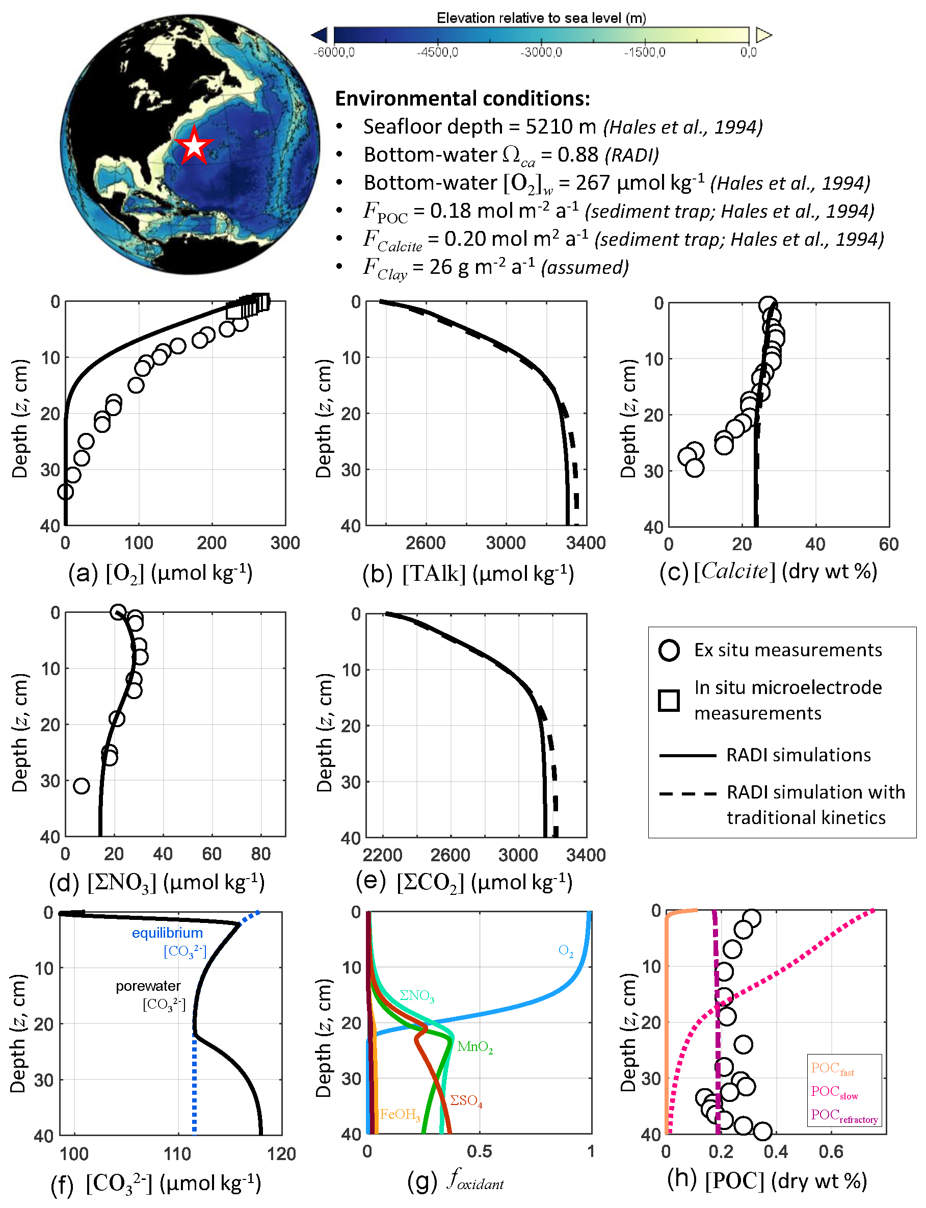
Figure 4 Comparison of RADI with measurements from the northwestern Atlantic station no. 9 described in Hales et al. (1994). The lower panels represent (f) the computed ${{\mathrm{CO}}_{\mathrm{3}}}^{\mathrm{2}-}$ concentrations in porewaters (solid black line) and at equilibrium with respect to calcite (dashed blue line) and (g) the fractions of organic matter degraded by a given oxidant.

3.2 Southern Pacific Ocean

RADI was also compared with data collected at the station no. 7 mooring no. 3 described in Sayles et al. (2001), located in the southern Pacific Ocean (60.15^∘ S, 170.11^∘ W), where the seafloor lies at a 3860 m depth. This dataset (http://usjgofs.whoi.edu/jg/dir/jgofs/southern/nbp98_2/, last access: 28 January 2022) constrains the sedimentary system well: sediment trap CaCO₃ and POC fluxes, CaCO₃, and POC sediment composition, sediment porosity, and porewater solute depth profiles are all available from the same cruise and location.

The bottom-water chemical composition was taken from the GLODAPv2 $\mathrm{1}{}^{\circ }\times \mathrm{1}{}^{\circ }$ climatologies (Lauvset et al., 2016), linearly interpolated over depth, latitude, and longitude to match the station location and seafloor depth. The bottom-water in situ temperature was 0.84 ^∘C, salinity was 34.696, oxygen concentration was 215.7 µmol kg⁻¹, and calculated saturation state with respect to calcite was 0.85. Solid fluxes at this station were measured by Sayles et al. (2001) using sediment traps collecting sinking particles between the months of November and December 1997. Their deepest sediment trap available was at a depth of 3257 m, i.e., 600 m a.s.f., which we assume to be representative of sinking fluxes to the seafloor, although the loss of material after collection usually causes sediment traps to underestimate the real sinking fluxes (Buesseler et al., 2007). The only CaCO₃ polymorph reaching the seafloor was assumed to be calcite, and its flux was set to 0.25 $\mathrm{mol}{\mathrm{m}}^{-\mathrm{2}}{\mathrm{a}}^{-\mathrm{1}}$ (25.02 $\mathrm{g}{\mathrm{m}}^{-\mathrm{2}}{\mathrm{a}}^{-\mathrm{1}}$), rather than using the sediment trap value, in order to fit the calcite sediment surface concentration measured by Sayles et al. (2001). This CaCO₃ flux to the seafloor is slightly higher than the measured CaCO₃ flux at 600 m above the seafloor in mid-January 1997 (0.19 $\mathrm{mol}{\mathrm{m}}^{-\mathrm{2}}{\mathrm{a}}^{-\mathrm{1}}$; Sayles et al., 2001). The POC flux was set to 0.14 $\mathrm{mol}{\mathrm{m}}^{-\mathrm{2}}{\mathrm{a}}^{-\mathrm{1}}$ (4.62 $\mathrm{g}\mathrm{OM}{\mathrm{m}}^{-\mathrm{2}}{\mathrm{a}}^{-\mathrm{1}}$), which is also slightly higher than the measured POC flux averaged between the months of November and December 600 m above the seafloor (0.11 $\mathrm{mol}{\mathrm{m}}^{-\mathrm{2}}{\mathrm{a}}^{-\mathrm{1}}$). The clay flux, which we considered to be the total measured sediment flux minus the assumed POC and calcite fluxes, was 32 $\mathrm{g}{\mathrm{m}}^{-\mathrm{2}}{\mathrm{a}}^{-\mathrm{1}}$. The porosity profile was tuned to best fit the porosity measurements at this station (Sayles et al., 2001, see Fig. 1). Finally, using the diffusive boundary layer world map computed in Sulpis et al. (2018) based on bottom current speeds at in situ temperature and pressure measurements, the diffusive boundary layer thickness (δ) at the station location was set to 715 µm. A complete description of the environmental parameters for this station, along with their sources, is available in Table S2 in the Supplement.

RADI was run using the environmental conditions described above to compare the steady-state concentration profiles of TAlk, ΣCO₂, O₂, ΣNO₃, calcite, and POC to in-situ measurements. Methods for solutes and solids concentration analyses are described in Sayles et al. (2001). Briefly, TAlk, ΣCO₂, and ΣNO₃ were sampled in situ using the Woods Hole Interstitial Marine Probe (Sayles, 1979), while O₂ was sampled at a higher depth resolution but in the ship laboratory using whole-core squeezing (Bender et al., 1987). We also compare the RADI steady-state concentration profiles with those obtained from a simulation with “traditional” 4.5-order calcite dissolution kinetics, all other variables being the same.

RADI predicts porewater O₂ concentrations that are slightly higher than observed (Fig. 5). Because RADI does not predict porewater O₂ to go to zero until about the 30 cm depth, the dominant organic matter degradation pathway switches from mainly aerobic to ΣNO₃ at about the 30 cm depth. Nevertheless, the RADI-predicted ΣNO₃ profile is lower than observed values, particularly toward the bottom of the resolved depth. The TAlk and ΣCO₂ porewater profiles predicted by a RADI simulation using 4.5-order calcite dissolution kinetics are slightly lower (≲40 µmol kg⁻¹) than those using the new calcite dissolution kinetics scheme, and the predicted calcite concentrations are slightly higher (≲2 %).

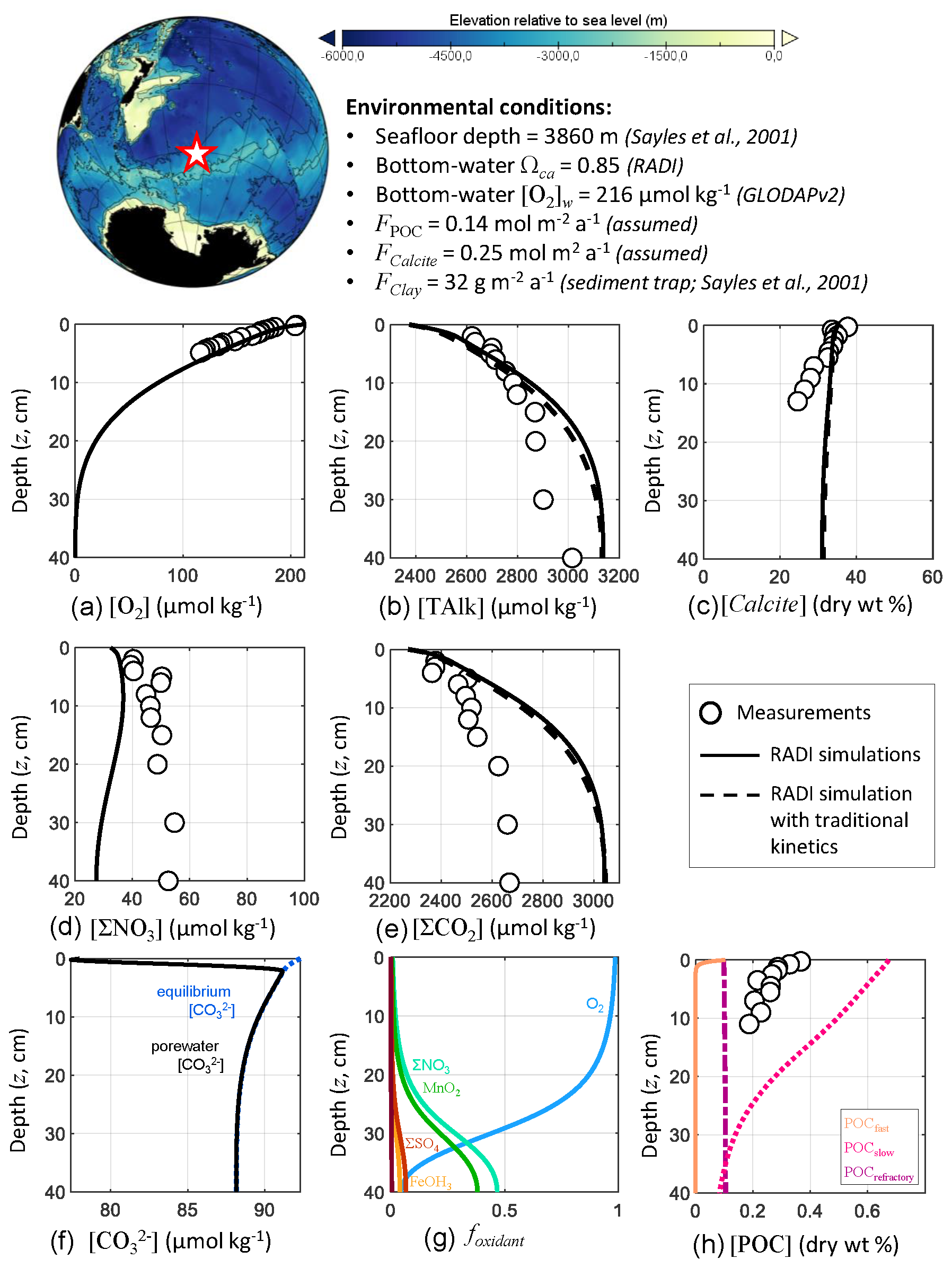
Figure 5 Comparison of RADI with measurements from the station no. 7 mooring no. 3 MC-1 described in Sayles et al. (2001). The lower panels represent (f) the computed ${{\mathrm{CO}}_{\mathrm{3}}}^{\mathrm{2}-}$ concentrations in porewaters (solid black line) and at equilibrium with respect to calcite (dashed blue line) and (g) the fractions of organic matter degraded by a given oxidant.

3.3 Central equatorial Pacific Ocean

As a third case study to evaluate the performance of RADI, solute fluxes through the sediment–water interface computed from model steady-state runs were compared to fluxes measured using benthic chambers. The comparison took place at station no. W-2 described in Berelson et al. (1994) and Hammond et al. (1996), located in the central equatorial Pacific Ocean (0^∘ N, 139.9^∘ W) at a depth of 4370 m. Bottom-water in situ temperature was set to 1.40 ^∘C and salinity was set to 34.69 (Lauvset et al., 2016). Bottom-water oxygen concentration was set to 159.7 µmol kg⁻¹ and the bottom-water saturation state with respect to calcite computed using the carbonate system solver within RADI was 0.78. For the purposes of this evaluation, the CaCO₃ flux to the seafloor was assumed to be entirely calcite. The calcite flux was set to 0.22 $\mathrm{mol}{\mathrm{m}}^{-\mathrm{2}}{\mathrm{a}}^{-\mathrm{1}}$, which represents 22.02 g of calcite m⁻² a⁻¹, the POC flux was 0.20 $\mathrm{mol}{\mathrm{m}}^{-\mathrm{2}}{\mathrm{a}}^{-\mathrm{1}}$, that is, 6.6 g of organic matter m⁻² a⁻¹, and the clay flux was set to 2.0 $\mathrm{g}{\mathrm{m}}^{-\mathrm{2}}{\mathrm{a}}^{-\mathrm{1}}$. The steady-state calcite content within the top centimeter was 61 dry wt %, in line with CaCO₃ contents observed in this area (Archer, 1996; Hammond et al., 1996). The porosity profile was built using an attenuation coefficient β=33 m⁻¹, φ₀=0.85, which is the measured surface porosity (Hammond et al., 1996), and φ_∞=0.74, which is the measured porosity at depth (Berelson et al., 1994); see Eq. (3). The DBL thickness, δ, was fixed to a value of 1 mm. A complete description of the environmental parameters for this station, along with their sources, is available in Table S3 in the Supplement.

The diffusive fluxes for a given solute (J_v) between the sediment–water interface and the bottom waters occur as a response to the concentration gradient within the DBL and can be expressed by

$$\begin{array}{}\text{(35)}& J_v={\mathit{\phi }}_{\mathrm{0}}{D}_v\times {\displaystyle \frac{v_{\mathrm{0}}-v_{\mathrm{w}}}{\mathit{\delta }}},\end{array}$$

where v₀ and v_w are solute concentrations at the sediment–water interface and in bottom waters, respectively. In this definition, a positive J_v indicates a solute release from the sediment porewaters to the bottom waters, while a negative J_v represents a solute flux towards the sediment.

The predicted TAlk, ΣCO₂, ΣPO₄, and O₂ fluxes (0.30 $\mathrm{mol}{\mathrm{m}}^{-\mathrm{2}}{\mathrm{a}}^{-\mathrm{1}}$, 0.32 $\mathrm{mol}{\mathrm{m}}^{-\mathrm{2}}{\mathrm{a}}^{-\mathrm{1}}$, 1.9 $\mathrm{mmol}{\mathrm{m}}^{-\mathrm{2}}{\mathrm{a}}^{-\mathrm{1}}$, and −0.23 $\mathrm{mol}{\mathrm{m}}^{-\mathrm{2}}{\mathrm{a}}^{-\mathrm{1}}$, respectively) are all within the uncertainty bounds of the fluxes measured by benthic chambers at the same location (0.28±0.09 $\mathrm{mol}{\mathrm{m}}^{-\mathrm{2}}{\mathrm{a}}^{-\mathrm{1}}$, 0.24±0.09 $\mathrm{mol}{\mathrm{m}}^{-\mathrm{2}}{\mathrm{a}}^{-\mathrm{1}}$, 1.4±0.5 $\mathrm{mmol}{\mathrm{m}}^{-\mathrm{2}}{\mathrm{a}}^{-\mathrm{1}}$, and $-\mathrm{0.26}\pm \mathrm{0.03}$ $\mathrm{mol}{\mathrm{m}}^{-\mathrm{2}}{\mathrm{a}}^{-\mathrm{1}}$, respectively; see Fig. 6). Nevertheless, the predicted ΣNO₃ flux (9.0 $\mathrm{mmol}{\mathrm{m}}^{-\mathrm{2}}{\mathrm{a}}^{-\mathrm{1}}$) is lower than its measured value (18±5 $\mathrm{mmol}{\mathrm{m}}^{-\mathrm{2}}{\mathrm{a}}^{-\mathrm{1}}$).

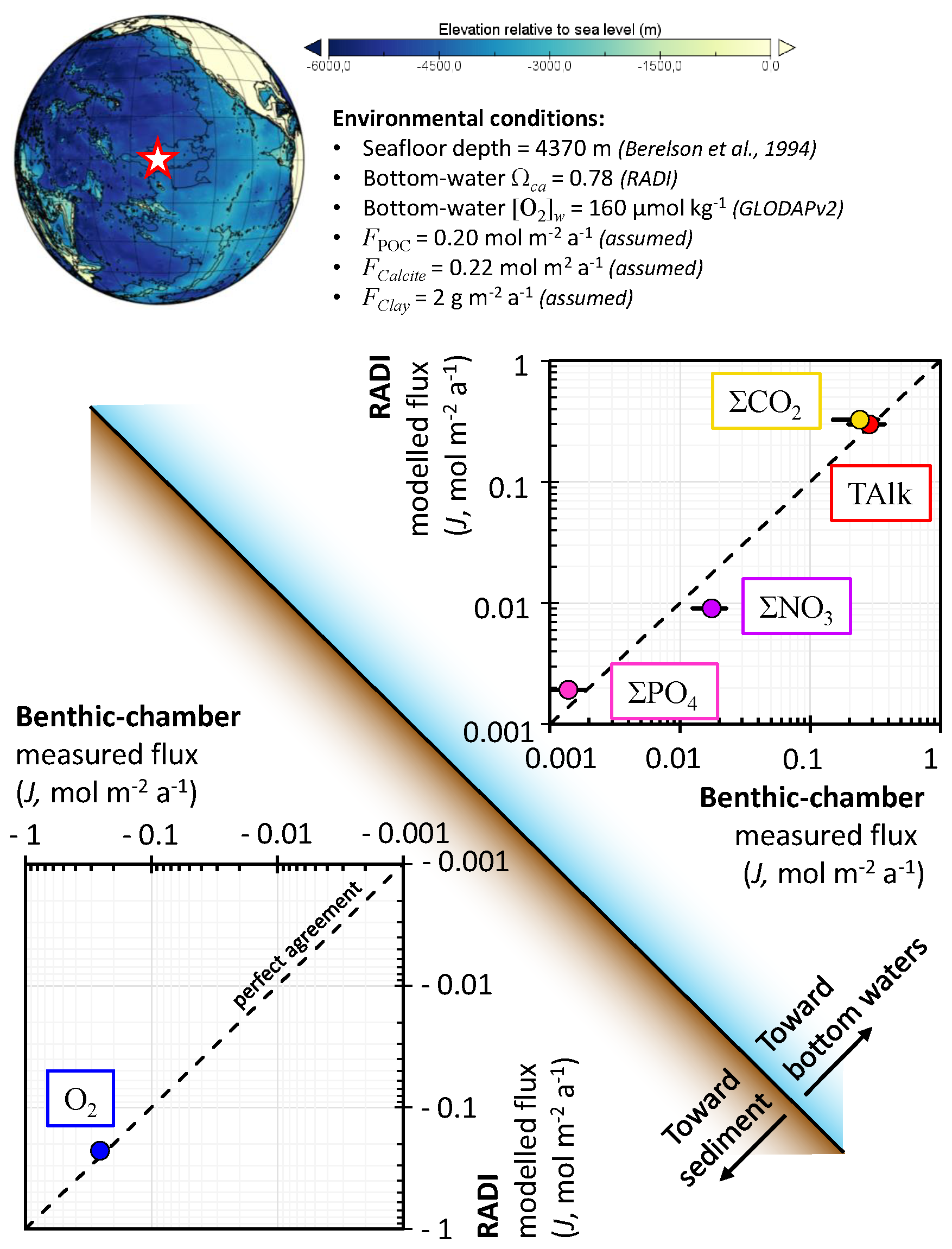
Figure 6 Comparison of fluxes computed from RADI with benthic-chamber measurements from the station no. W-2 described in Hammond et al. (1996). Error bars are included for all measured fluxes but are not always visible.

3.4 Discussion of model performance

These three model evaluation examples allowed us to determine a set of organic carbon degradation rate constants, CaCO₃ dissolution rate constants and organic carbon flux composition (fast-decay, slow-decay, or refractory) that can best reproduce sediment and porewater measurements in all stations while keeping all other model parameters to values from the literature. In each station, bottom-water composition was fixed from observations. Due to a lack of adequate data, solid deposition fluxes were tuned to best fit observed CaCO₃ and POC contents in sediments, except in the northwestern Atlantic station, where the CaCO₃ and POC fluxes were taken from measurements, and in the southern Pacific station, where the clay flux was inferred from observations. The POC composition that allows to best fit porewater and sediment data in the three stations was as follows: 70 % of fast-decay POC, 27 % of slow-decay POC, and 3 % of refractory POC. The tuned fast- and slow-decay POC degradation rate constants are reported in Sect. 2.2.1 and are of similar orders of magnitude as in most other models (Arndt et al., 2013). The tuned CaCO₃ dissolution rate constants are reported in Sect. 2.2.3 and are 2 orders of magnitude lower than their laboratory-based values (Fig. S1), which we attribute to the presence of dissolution inhibitors (e.g., dissolved organic carbon, Naviaux et al., 2019a) or to the reactive surface area of natural grains in situ being lower than in laboratory experimental settings. Thus, with its current settings, RADI should be able to accurately predict porewater chemistry and sediment composition in deep-sea environments, provided that the POC and CaCO₃ deposition fluxes are known.

In the central equatorial Pacific, all RADI diffusive fluxes are within the uncertainty range of observations except the ΣNO₃ flux, which is underestimated by RADI. The low ΣNO₃ flux could be attributed, for example, to the presence of organic matter with a stoichiometry different than the Redfield ratio used in the current version of RADI or to errors in the nitrification parameters.

In addition, we note that the choice of calcite dissolution kinetics implemented in RADI does not seem to have a large impact on TAlk and ΣCO₂ porewater profiles or on the predicted calcite concentrations. RADI's step-edge retreat dissolution regime and its low reaction order induce calcite dissolution rates near equilibrium that are orders of magnitude higher than what is predicted in a high-order rate law (Fig. 2), but if the rate constant of a high-order rate law is tuned so that it overlaps the homogeneous dissolution rate law far from equilibrium, differences are limited (Fig. 2). Thus, we conclude that using a 4.5-order rate law with a 10 % d⁻¹ rate constant or using the new, mechanistic calcite dissolution rate scheme implemented in RADI should lead to similar predictions.

4 Potential model applications

In the following section, we continue to analyze the results obtained using the environmental conditions of the equatorial Pacific station no. W-2 and present a few examples of relevant model applications. RADI can be used to study both steady-state and transient conditions, but in the following subsections we focus on time-dependent problems, since transient diagenetic models are underrepresented in the literature.

4.1 Seasonal variability

At the seafloor, the fluxes of sinking material regulating the chemical composition of sediment porewaters are patchy in both space and time. Seafloor microbes and macrofauna respond quickly to pulses of organic matter delivery to the seafloor (Smith et al., 1992), causing short-term variability of sediment oxygen consumption (Smith and Baldwin, 1984; Smith et al., 1994). In addition, both the POC and CaCO₃ fluxes to the deep seafloor are strongly affected by seasonal flux variability (Billett et al., 1983; Smith and Baldwin, 1984; Lampitt, 1985; Lampitt et al., 1993, 2010). In the northeastern Atlantic Ocean at 3000 m depth, Lampitt et al. (2010) have shown that the summer POC and CaCO₃ fluxes can be ∼10 and ∼4 times higher, respectively, than the wintertime minima. The seasonal coupling between organic matter and CaCO₃ fluxes to the seafloor and the state of upper-ocean ecosystem is the result of rapid vertical transport of these materials (Sayles et al., 1994). If the fluxes of reactive material reaching the seafloor are affected by seasons, early diagenesis could display a seasonal signal, and this should be taken into account when interpreting sedimentary data (Martin and Bender, 1988; Sayles et al., 1994; Soetaert et al., 1996a). Here we use RADI to assess how the porewater chemistry and solid composition of deep-sea sediments may be impacted by seasonally varying fluxes.

Seasonally time-varying solid fluxes to the seafloor (F, in $\mathrm{mol}{\mathrm{m}}^{-\mathrm{2}}{\mathrm{a}}^{-\mathrm{1}}$) can be represented with the following sinusoidal function:

$$\begin{array}{}\text{(36)}& F\left(t\right)=F_{\text{average}}+\mathrm{\Delta }F\sin \left({\displaystyle \frac{\mathrm{2}\mathit{\pi }t}{\mathrm{\Delta }t}}\right),\end{array}$$

where t is time in years, Δt is the time period separating two maxima (here set to 1 year), and ΔF is the amplitude. We assume that all CaCO₃ settling at the seafloor is calcite and set the mean F_Calcite to 0.22 $\mathrm{mol}{\mathrm{m}}^{-\mathrm{2}}{\mathrm{a}}^{-\mathrm{1}}$, its amplitude change ΔF_Calcite to 0.11 $\mathrm{mol}{\mathrm{m}}^{-\mathrm{2}}{\mathrm{a}}^{-\mathrm{1}}$, the mean F_POC to 0.20 $\mathrm{mol}{\mathrm{m}}^{-\mathrm{2}}{\mathrm{a}}^{-\mathrm{1}}$, and its amplitude change ΔF_POC to 0.10 $\mathrm{mol}{\mathrm{m}}^{-\mathrm{2}}{\mathrm{a}}^{-\mathrm{1}}$. All other parameters correspond to values from the central equatorial Pacific stations described in Sect. 3.3.

Seasonal variations in the calcite and POC fluxes reaching the seafloor are visible in sediment profiles of both solids and solutes (Fig. 7). Nonetheless, the amplitude of concentration changes separating an annual minimum from an annual maximum is very small, barely if (at all) detectable by observations. The annual amplitude is about 0.5 wt % for calcite, 0.07 wt % for POC, 2 µmol kg⁻¹ for [O₂], and 7 µmol kg⁻¹ for [ΣCO₂]. While concentrations at the sediment–water interface respond quickly to seasonal flux changes, there is a phase lag that increases with depth between the concentrations of solids and porewater solutes and the seasonally changing fluxes to the seafloor. Thus, it is possible that porewaters and solid particles at the top millimeter-thick sediment layers are never really at a steady state but always lagging behind seasonal changes, even if these are minimal. This is in agreement with earlier modeling (Martin and Bender, 1988) and observational (Sayles et al., 1994) studies, indicating that biogeochemical reactions and bioturbation at the deep seafloor are too slow to show a discernible seasonal signal. However, this might not be the case for sites receiving more reactive organic matter (Soetaert et al., 1996a).

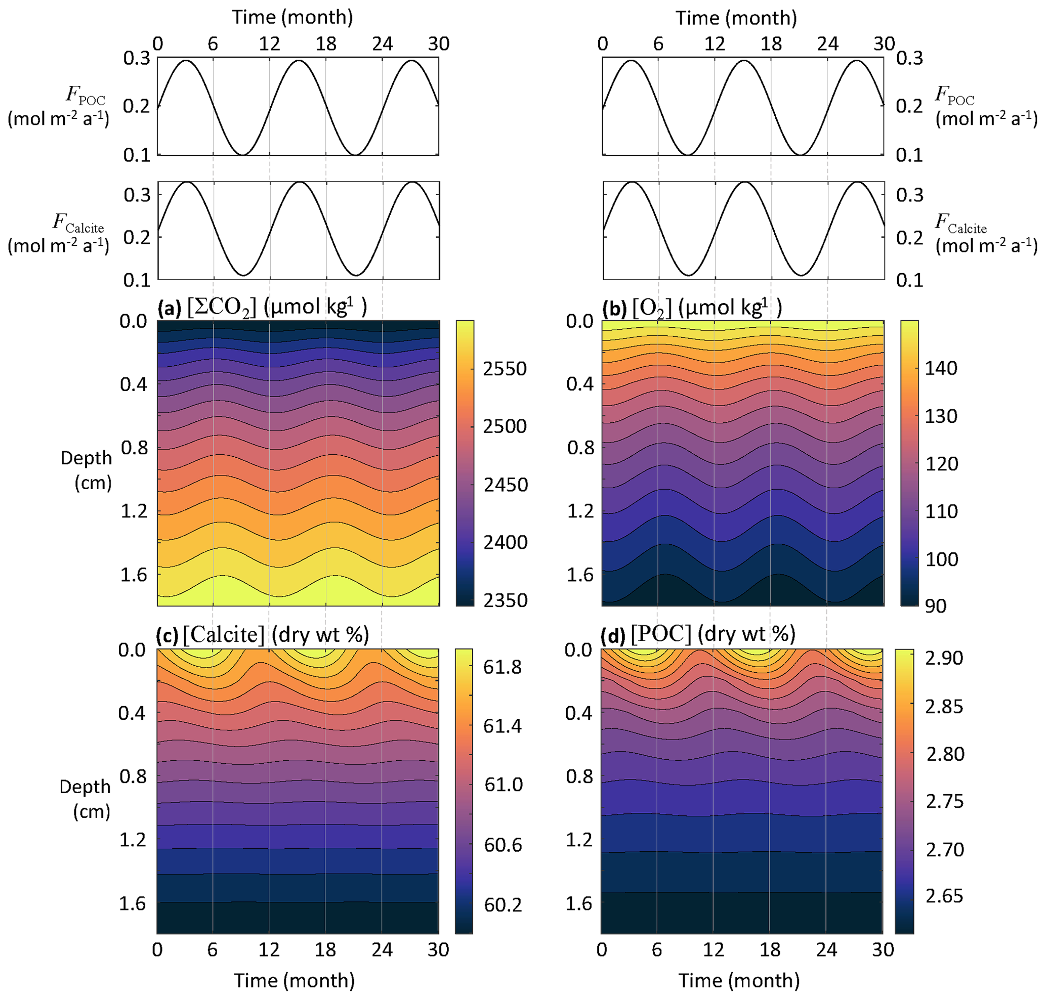
Figure 7 Response of porewater O₂, ΣCO₂, calcite, and POC concentrations to seasonal fluctuations in the calcite and POC fluxes reaching the seafloor.​​​​​​​

4.2 Tidal cycles

This section explores the applicability of RADI for studying the response of sediments to higher-frequency phenomena such as tides. The DBL thickness is dependent on the overlying current speed (Levich, 1962; Santschi et al., 1983; Lorke et al., 2003): slower currents generate thicker DBLs, whereas faster currents cause the DBL to thin (Larkum et al., 2003; Lorke et al., 2003; Higashino and Stefan, 2004). In the deep sea, tidal forces are an important contributor to benthic current speeds, which means that tidal currents are a potentially important contributor to biogeochemical exchanges across the sediment–water interface (Egbert and Erofeeva, 2002; Sulpis et al., 2019). If tidal current speed fluctuations induce DBL thickness fluctuations, they may induce solute concentration fluctuations at the sediment–water interface, thus affecting early diagenesis. The strongest tidal currents occur during the transition from high to low tides. For semidiurnal tides, the time period separating a low from a high tide is ∼6 h (Pugh, 1987). Setting the average DBL thickness to δ=1 mm and assuming that tides generate δ fluctuations with an amplitude Δδ=0.5 mm, the time-dependent δ can be expressed as follows:

$$\begin{array}{}\text{(37)}& \mathit{\delta }\left(t\right)={\mathit{\delta }}_{\text{average}}+\mathrm{\Delta }\mathit{\delta }\sin \left({\displaystyle \frac{\mathrm{2}\mathit{\pi }t}{\mathrm{\Delta }t}}\right),\end{array}$$

where t is time in years and Δt is set to $\mathrm{1}/\mathrm{1461}$ a (∼6 h). RADIv1 was run using the steady-state solutes and solids depth profiles from the equatorial Pacific station no. W-2 as initial conditions, with a DBL thickness fluctuating in response to tidal currents computed using Eq. (37).

While none of the solids seem to respond to tidal velocity fluctuation due to their slow accumulation rate, solutes show a clear response (Fig. 8). At the sediment–water interface, the simulated porewater [ΣCO₂] variation amplitude within a single tidal cycle is about 25 µmol kg⁻¹, while [O₂] oscillates with an amplitude of about 8 µmol kg⁻¹. Deeper than a few millimeters below the sediment–water interface, the amplitude of both [ΣCO₂] and [O₂] changes become very small and tidal cycles are not measurable in the concentration profiles.

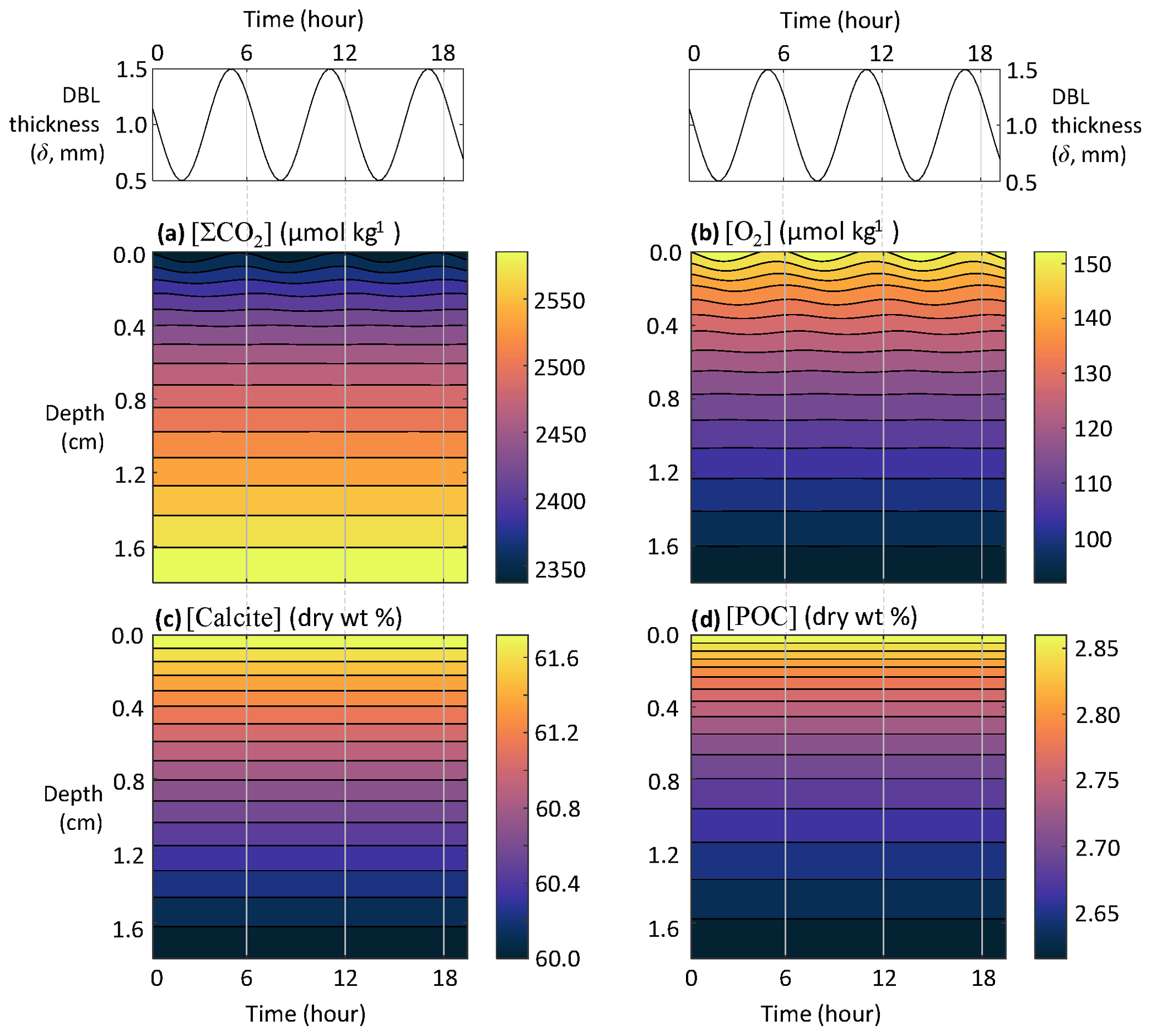
Figure 8 Response of porewater O₂, ΣCO₂, calcite, and POC concentrations to fluctuations in DBL thickness (δ) driven by tidal currents.

The implications are potentially important for our interpretation of porewater microprofiles. Profiles of pH (Archer et al., 1989b; Cai and Reimers, 1993; Zhao and Cai, 1999; Cai et al., 2000); pCO₂ (Cai et al., 2000; Zhao and Cai, 1997); ${{\mathrm{CO}}_{\mathrm{3}}}^{\mathrm{2}-}$ (de Beer et al., 2008; Han et al., 2014; Cai et al., 2016); O₂ (Revsbech et al., 1980; Reimers, 1987; Archer et al., 1989a; Sosna et al., 2007); and even dissolved Fe, Mn, or S(-II) (Brendel and Luther, 1995) microelectrodes have been developed during the past decades. According to the results presented here, microprofiles, which capture instantaneous snapshots of porewater chemistry, should show appreciable differences depending on when they are carried out during a tidal cycle. That organic matter degradation rates inferred from oxygen microprofiles span a wide range (Archer et al., 1989a; Arndt et al., 2013; Wenzhöfer et al., 2016) may be, among other factors, due to the dependency on tidal and other ocean bottom current fluctuations. To adequately capture O₂ consumption rate in sediments, O₂ fluxes should be measured and integrated over a period of time longer than a tidal cycle (Berg et al., 2022).

4.3 Benthic chambers

RADI can also be used in the calibration of sensors and the optimization of sampling protocols and experimental designs. In the DBL, molecular diffusion is the dominant mode of solute transport, and laboratory experiments of CaCO₃ dissolution in seawater suggest that diffusion through the DBL is the rate-limiting step for CaCO₃ dissolution at the seafloor in the absence of organic matter respiration (Sulpis et al., 2017; Boudreau et al., 2020). Nevertheless, earlier assessments of in situ CaCO₃ dissolution at the sediment–water interface in the central equatorial Pacific indicated that DBL thickness does not impact overall dissolution rates (Berelson et al., 1994).

In their study, Berelson et al. (1994) deployed a set of free-sinking benthic chambers onto the seafloor. In each chamber, the portion of the chamber exposed above the sediment–water interface was sealed and isolated from external bottom waters, and water samples were drawn during the incubation period. Each incubation lasted between 80 and 120 h. Chambers were stirred with a paddle at various rates to quantify the dependency of the measured diffusive fluxes across the sediment–water interface on the DBL thickness, which were calibrated via anhydrite dissolution to the 300–600 µm range. Seeing no influence of the stirring rate on the measured diffusive fluxes, Berelson et al. (1994) discarded the hypothesis of fast, surficial carbonate dissolution and instead argued for slow, high reaction order calcite dissolution kinetics at the seafloor, as subsequently implemented in most models. To better interpret the results from a benthic-chamber study such as that of Berelson et al. (1994), RADI can be used to predict the time response of diffusive fluxes across the DBL following an instantaneous change of DBL thickness due to, for instance, a change in paddle stirring rate within a chamber.

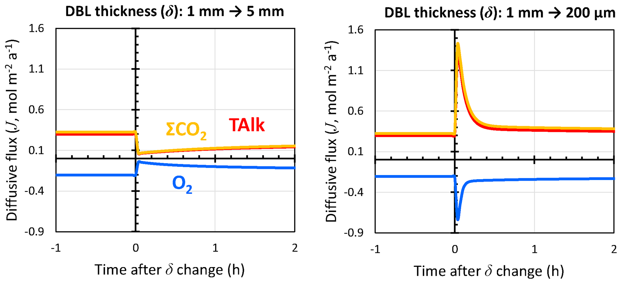
Figure 9 Response of TAlk, ΣCO₂, and O₂ diffusive fluxes through the DBL to instantaneous changes in the DBL thickness (δ) as caused by, for instance, a stirred benthic chamber. Positive values represent solute fluxes toward the bottom waters, while negative values represent solute fluxes toward the sediments.

RADI was run using the steady-state solutes and solids depth profiles from the equatorial Pacific station no. W-2 as initial conditions. In the initial run, the DBL thickness was set to 1 mm. We simulated the response of this sediment to an instantaneous change in the DBL thickness, with one model run representing a situation where δ increases from 1 to 5 mm (e.g., a slow stirring rate) and one model run representing a δ drop from 1 mm to 200 µm (e.g., a fast stirring rate). Following a 5-fold increase in δ, diffusive fluxes of TAlk, ΣCO₂, and O₂ initially decrease by a factor ∼5 but then increase back as the solute concentrations at the interface adapt to the new DBL (Fig. 9). A total of 2 h after the δ increase, diffusive fluxes converge toward a new steady state. Following a 5-fold decrease in δ, diffusive fluxes immediately increase by the same magnitude but go back to close to their initial value within an hour as the interfacial porewater concentrations adjust to the new DBL. These results suggest that the incubation periods of the Berelson et al. (1994) benthic-chamber experiments were long enough to let porewaters adjust to the changes caused by the paddle stirrers and confirm that, in sediment rich in organic matter and CaCO₃ such as that of the Equatorial Pacific, the influence of a DBL on diffusive fluxes across the sediment–water interface should indeed be limited. Additionally, these results confirm the observation by Berelson et al. (1994) that changing the stirring rate in a benthic chamber does not alter steady-state diffusive fluxes by much under the CaCO₃ and POC deposition fluxes encountered in the equatorial Pacific. Part of the reason may be the quick adjustment of porewater concentrations to the new diffusive boundary layer (see Fig. S3 in the Supplement).

4.4 Additional applications

The time-dependent problems presented above focus on relatively short timescales (from minutes to months). A non-steady-state model such as RADI can also be used to project the sediment response to perturbations over longer periods of time. Examples include estimating the effect of negative emission technologies, such as coastal enhanced weathering with olivine on early diagenesis (Meysman and Montserrat, 2017; Montserrat et al., 2017), deep-sea mining (Haffert et al., 2020), or bottom trawling (Trimmer et al., 2005; van de Velde et al., 2018; De Borger et al., 2021); the impacts of a decadal bottom-water deoxygenation event such as in the Saint Lawrence estuary (Jutras et al., 2020); or the present anthropogenic CO₂ transient. However, the current version of RADI cannot deal with long-term major dissolution (erosion) events because the burial velocity calculation scheme currently implemented does not account for solid mass gain or loss within the sediment. To study the response of sediments to a global-scale, long-duration ocean acidification event such as the Paleocene–Eocene Thermal Maximum (Zachos et al., 2005; Cui et al., 2011), a different burial velocity calculation scheme would have to be implemented, such as that adopted by Munhoven (2021).

5 Future developments

One advantage of RADI is that it is easily tunable by the user: adding new components is straightforward as long as the chemical reactions are known. In future releases, we plan to add oxygen, carbon, and calcium isotopes as individual components in order to predict the diagenetic response of isotopic signals. Additionally, adsorption and desorption reactions on clay surfaces could be a critically important advance, especially regarding the prediction of sedimentary pH profiles (Meysman et al., 2003), as RADI currently treats clay minerals as non-reactive.

The representation of organic matter in the current version of the model is oversimplified. All reactive organic matter in RADI is associated with a Redfield stoichiometry, but marine organic matter can considerably deviate from this ideal (Martiny et al., 2013; Teng et al., 2014).

Finally, a model is only as good as its assumptions. RADI is targeted to study deep-sea, carbonate sediments. To be used in coastal environments, additional biogeochemical reactions would be necessary, particularly those involving methane and iron sulfide. Close to the shore, sediments become more permeable, and the assumption of molecular diffusion as the dominant mode of solute transport in porewaters does not hold. In very shallow environments that are subject to high wave energy, pressure-induced advection in the sediment porewaters also needs to be included (Huettel et al., 2014). Moreover, coastal sediments typically have lower pH than open-ocean sediments, which may render our assumption of both ΣCO₂ and TAlk diffusing with a fixed diffusion coefficient set to that of the ${{\mathrm{HCO}}_{\mathrm{3}}}^{-}$ ion inaccurate; see Fig. S2. Other chemical species (e.g., dissolved sulfide, ammonium) that also contribute to the measured pore water alkalinity may also invalidate this assumption.