the Creative Commons Attribution 4.0 License.
the Creative Commons Attribution 4.0 License.
 | 18 Feb 2022
Mapping high-resolution basal topography of West Antarctica from radar data using non-stationary multiple-point geostatistics (MPS-BedMappingV1)
Chen Zuo
Emma J. MacKie
The subglacial bed topography is critical for modelling the evolution of Thwaites Glacier in the Amundsen Sea Embayment (ASE), where rapid ice loss threatens the stability of the West Antarctic Ice Sheet. However, mapping of subglacial topography is subject to uncertainties of up to hundreds of metres, primarily due to large gaps of up to tens of kilometres in airborne ice-penetrating radar flight lines. Deterministic interpolation approaches do not reflect such spatial uncertainty. While traditional geostatistical simulations can model such uncertainty, they become difficult to apply because of the significant non-stationary spatial variation of topography over such large surface area. In this study, we develop a non-stationary multiple-point geostatistical (MPS) approach to interpolate large areas with irregular geophysical data and apply it to model the spatial uncertainty of entire ASE basal topography. We collect 166 high-quality topographic training images (TIs) of resolution 500 m to train the gap-filling of radar data gaps, thereby simulating realistic topography maps. The TIs are extensively sampled from deglaciated regions in the Arctic as well as Antarctica. To address the non-stationarity in topographic modelling, we introduce a Bayesian framework that models the posterior distribution of non-stationary TIs assigned to the local line data. Sampling from this distribution then provides candidate training images for local topographic modelling with uncertainty, constrained to radar flight line data. Compared to traditional MPS approaches that do not consider uncertain TI sampling, our approach results in a significant improvement in the topographic modelling quality and efficiency of the simulation algorithm. Finally, we simulate multiple realizations of high-resolution ASE topographic maps. We use the multiple realizations to investigate the impact of basal topography uncertainty on subglacial hydrological flow patterns.
- Article
(43257 KB) - Full-text XML
- BibTeX
- EndNote


The topography beneath the Greenland and Antarctic ice sheets is essential for nearly every ice sheet investigation, including modelling subglacial hydrology (e.g. De Fleurian et al., 2018; MacKie et al., 2021a; Siegert et al., 2016; Sommers et al., 2018), interpreting geologic conditions (Bingham and Siegert, 2009; King et al., 2009; Rippin et al., 2014; Holschuh et al., 2020; Alley et al., 2021), estimating ice volume and sea level rise contributions (e.g. Fretwell et al., 2013; Morlighem et al., 2020) and ice sheet modelling for sea level rise projections (e.g. Le clec'h et al., 2019; Schlegel et al., 2018; Seroussi et al., 2017). The characterization of subglacial topography is particularly important for Thwaites Glacier in the Amundsen Sea Embayment, which is experiencing accelerating ice loss (Rignot et al., 2019) that could destabilize the West Antarctic Ice Sheet (Joughin et al., 2014). Subglacial topography is predominantly measured with airborne ice-penetrating radar along flight lines separated by up to tens of kilometres (e.g. Bingham et al., 2017; Fretwell et al., 2013; Herzfeld et al., 1993). Large gaps in data remain, which are generally interpolated deterministically using methods such as kriging (Herzfeld et al., 1993), the ArcGIS Topogrid algorithm (Fretwell et al., 2013), spline interpolation (Lytheand Vaughan, 2001; Holt et al., 2006) or ice sheet model inversions (Farinotti et al., 2017; Huss and Farinotti, 2012; Morlighem et al., 2017, 2020). These approaches produce topography that is unrealistically smooth and provide limited morphological information. Furthermore, deterministically interpolated topography does not sample the uncertainty space, making it difficult to quantify uncertainty in ice sheet models with respect to topographic uncertainty. These issues have previously been addressed with two-point geostatistical simulation, such as fast Fourier transforms (Goff et al., 2014; Graham et al., 2017; MacKie et al., 2020) or sequential Gaussian simulation (SGSIM) (MacKie et al., 2021a). The objective of geostatistical simulation is to generate multiple realizations of phenomena that reproduce the spatial variability of observations, as modelled by variogram or spatial covariance and can be used to quantify uncertainty (e.g. Deutsch and Journel, 1998). Goff et al. (2014) also conducted a conditional simulation of Thwaites Glacier. To improve the modelling quality, the channelized structures and the abrupt transition between lowland and highland are individually handled. The method has the advantage to ensure the continuity of fjord-like channels beneath the glacier. Geostatistical simulation has also been applied in Antarctica and Greenland to quantify uncertainty in subglacial hydrology (MacKie et al., 2020, 2021a; Zuo et al., 2020).
However, spatial variation over very large areas is inherently non-stationary. For example, the Greenland and Antarctic ice sheets are thousands of kilometres in length and contain a wide range of topographic and geologic settings. This means that the nature of spatial variation changes significantly and possibly in complex ways over the domain of interest. Traditional geostatistical ways of dealing with non-stationary data are through the modelling of trend functions (e.g. Pyrcz and White, 2015) or using covariates (e.g. Almeida and Journel, 1994; MacKie et al., 2021a). However, such approaches typically model the variation in the mean (trend) or some degree of correlation (co-simulation). Another approach is using a non-stationary spatial covariance model (Schmidt and O'Hagan, 2003). Such an approach becomes exceedingly difficult to apply over large areas because of the use of Markov chain Monte Carlo in its Bayesian inference. Regardless, most two-point geostatistical approaches are limited in expressing non-stationarity in terms of a mean or covariance function only.
The non-stationary bed topography is measured using high-resolution remote sensing data such as satellite imagery but only in deglaciated areas (Porter et al., 2018). Deglaciated topographic images reveal glaciated morphologies resembling the topography beneath the contemporary ice sheets (King et al., 2009; Margold et al., 2015; Spagnolo et al., 2017). They therefore bear significant morphological information on the subglacial topography. Exposed topography has previously been used to perform deterministic interpolations (Clarke et al., 2009). However, deglaciated topography has not been used to stochastically simulate subglacial topography, until the very recent alpine glacier study by Neven et al. (2021) using multiple-point geostatistics.
Recent developments in multiple-point geostatistics (MPS) has shown great potential in using high-resolution training images (e.g. satellite images) to fill remote sensing gaps (e.g. Gravey and Mariethoz, 2020; Mariethoz et al., 2012; Yin et al., 2017; Zakeri and Mariethoz, 2021; Zuo et al., 2020). MPS approaches use the training images (TIs) as explicit prior models to generate realistic topographical models and quantify spatial uncertainty. The simulation of non-stationary and morphologically complex topography can also be achieved with MPS (Hoffimann et al., 2017, 2019; Mariethoz and Caers, 2014). Compared to alternative machine learning or deep learning approaches (Laloy et al., 2018; Mo et al., 2020), MPS has a flexible conditioning capability and can accommodate sparse and non-uniform sampling in space. It can generate multiple topographic model realizations conditioned to the radar line observations, without requiring a large amount of training data.
We briefly review three categories of approaches to build non-stationary geospatial models using MPS. The first way is to divide non-stationary TI or simulation grid into several stationary subareas. Each stationary simulation area has its specified stationary TI (Honarkhah and Caers, 2012; Strebelle, 2002; Wu et al., 2008; Zhou et al., 2014). However, the zonation may create artefacts in areas where two zones meet. Therefore, the second way is most commonly used. It incorporates spatially continuous non-stationary maps (named as “auxiliary variables”) with weighted aggregation or so-called “ad-hoc weighting” (Chugunova and Hu, 2008; Mariethoz et al., 2010; Oriani et al., 2014; Zuo et al., 2020). Such auxiliary variables determine which TI patterns should fill which location in the simulation domain in a spatially smooth manner. The limitation is that the ad-hoc weights do not scale to the complexity of bed topography. The determination of weights is also subjective. Moreover, auxiliary variables are very difficult to obtain in subglacial topographic modelling. Another challenge in the non-stationary modelling is how to choose training images (Tahmasebi, 2018). This is particularly important as the MPS modelling relies on the spatial information provided by the training images. In the third option, Hoffimann et al. (2019) introduced an approach to generate time-series training images to model the spatial and temporal evolutions of geomorphology, which is similar to Pirot et al. (2014, 2015). A training image transitional model in time was proposed to reproduce the non-stationary geomorphologic evolutions. However, in subglacial topographic modelling, there is limited training imagery because subglacial topographic measurements are only made along flight lines. Graham et al. (2017) provided a synthetic bed elevation terrain for Antarctica. Satellite-based observations from deglaciated areas in the Arctic offer a potential source of training imagery. But these Arctic training images would be non-stationary due to the natural variability of the landscape. Furthermore, the Arctic provides a vast amount of deglaciated topographic data, which present a significant computational burden on MPS simulation algorithms. We therefore need a strategy to explicitly specify which training images or patterns should go where when filling the radar line gaps.
In this paper, we generalize a geospatial modelling framework to fill irregular geophysical data gaps in large areas. We use MPS to address the non-stationary topographic modelling by probabilistically selecting non-stationary training images. We first collect a large number of TIs from the deglaciated areas in the Arctic and Antarctica. Then we develop a probability aggregation method to estimate each TI's probability of being assigned to different local radar lines. This probabilistic TI selection scheme avoids the use of auxiliary variables with arbitrary ad-hoc weighting. We demonstrate our method using the entire Amundsen Sea Embayment (ASE) in West Antarctica. This region has alternating areas of sparse and dense measurements with a variety of radar line orientations. We show that the training image sampling process accommodates a range of data configurations. We generate realistic non-stationary topographic realizations that reflect the subglacial topographic uncertainty in ASE. We then use the topographic simulations to model subglacial hydrologic flow in order to investigate the impact of topographic uncertainty on hydrologic uncertainty.
The topographic data for the ASE include seafloor bathymetry measurements from the International Bathymetric Chart of the Southern Ocean (IBCSO) (Arndt et al., 2013), subaerial topography from the Reference Elevation Model of Antarctica (REMA) (Howat et al., 2019), and ice-penetrating radar measurements of subglacial topography (Blankenship et al., 2001; Gogineni, 2012; Holschuh et al., 2020; Holt et al., 2006; Vaughan et al., 2006; Young et al., 2016). The data are gridded at a 500 m spatial resolution by averaging the measurements within each grid cell (Fig. 1). The swath bathymetry data (Arndt et al., 2013) and subglacial swath radar data (Holschuh et al., 2020) provide some training imagery. To have more extensive representations of the subglacial topography, we increase the available training data with deglaciated subaerial topography from ArcticDEM V3 (Porter et al., 2018). The Arctic and much of North America were formerly covered by the Laurentide and Cordilleran ice sheets and share morphological similarities with Antarctic subglacial topography (King et al., 2009; Margold et al., 2015). While the seafloor and subaerial topography may have experienced additional erosional and depositional processes after deglaciation, any topographic alterations are likely minimal at a 500 m resolution. We sampled a total 166 candidate training images to capture a variety of geological settings (Fig. 2). Each training image has a size of 100 km × 100 km. The training image data repository is publicly accessible on the Zenodo repository (https://zenodo.org/record/5083715#.YQT2JI5Kiiw (last access: 8 July 2021), https://doi.org/10.5281/zenodo.5083715, MacKie et al., 2021b).
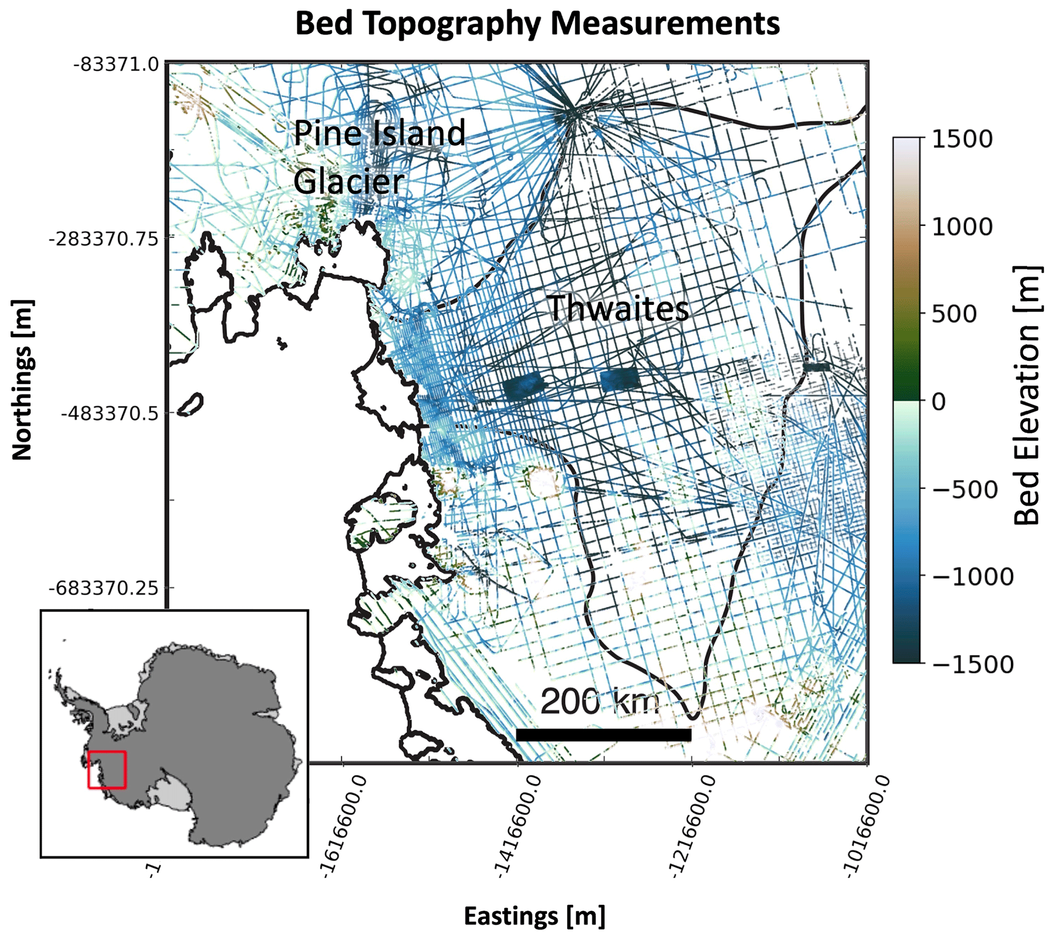
Figure 1Radar line surveys of the Thwaites and Pine Island glaciers in the Amundsen Sea Embayment of West Antarctica. The red box implies the location of the study area in Antarctica. Black lines indicate boundaries for Thwaites Glacier, ice shelves, and the grounding line (the point where the ice detaches from the bed and achieves flotation). The two topography patches in the centre of Thwaites Glacier were measured using swath radar (Holschuh et al., 2020).
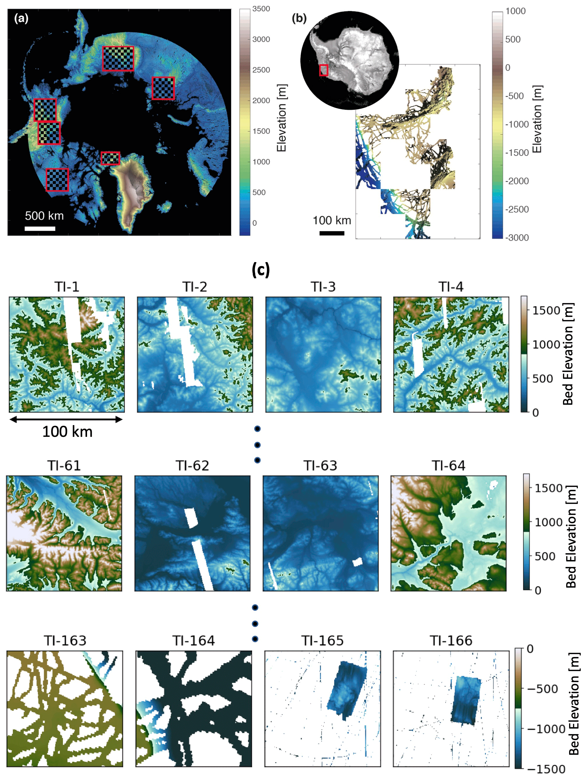
Figure 2Geographical locations of the 166 training images in (a) ArcticDEM (red boxes encompass TI regions) and (b) Antarctica's Amundsen Sea Embayment region. (c) Examples of the 166 training images.
3.1 Multiple-point geostatistics
3.1.1 Overview
Multiple-point geostatistics (Journel and Zhang, 2006; Mariethoz and Caers, 2014; Srivastava, 2018; Strebelle, 2002) is the field of study that focuses on the digital representation of physical reality by reproducing high-order statistics inferred from training images. The emphasis in MPS lies on capturing higher order (hence multi-point statistics) from training images that have been selected to be representative for a specific area of study. In that sense, it differs from spatial covariance-based (variograms) methods (e.g. Gaussian process regression or kriging) (Matheron, 1963; Williams and Rasmussen, 1996) that are based on spatial correlation (two values at a time). Both MPS and covariance-based methods have the ability to interpolate data exactly at the data locations. Exact interpolation, if desired, is also where geostatistics differs from machine learning or computer vision methods, where such exact interpolation is not usually considered important.
Several MPS simulation algorithms (e.g. Gravey and Mariethoz, 2020; Hoffimann et al., 2017; Mariethoz et al., 2010; Strebelle and Journel, 2001) have been developed that use training images to generate multiple realizations that interpolate the data exactly. The algorithm used in this work is direct sampling (DS) (Mariethoz et al., 2010; Mariethoz and Renard, 2010), which will be introduced in the following section. These algorithms do not address the challenge of selecting the training images themselves. For example, if an area of the simulation grid contains dense data, few training images may be compatible with those data. On the other hand, an area with sparse data may have many compatible training images. Finally, training images selected for two adjacent areas are not necessarily independent from each other.
To date, there has not been any attempt to use MPS to interpolate ice-penetrating radar measurements of topography at the scale of the Amundsen Sea Embayment. In doing so, additional challenges occur that are not present in smaller study areas. The challenges may include limited number of training images, non-stationarity over the ASE, and running time cost when generating high-resolution topographic maps. Before moving to the methodology that addresses these challenges, we first introduce the direct sampling method and a probabilistic framework for representing training images in metric spaces.
3.1.2 Direct sampling
Direct sampling is a widely used MPS approach for achieving spatial modelling and gap filling (Mariethoz, 2018; Mariethoz et al., 2012; Zuo et al., 2020). Figure 3 provides a simplified example of DS in the context of flight lines. The values in the grid indicate the elevation. In general, there are two major components within DS. First, the algorithm visits an unknown location in the simulation grid and collects neighbouring observed points as conditioning data. For example, in Fig. 3a, three conditioning points are detected near an unknown location (marked with “?”). DS records the values and relative locations of known points. Second, a searching programme is launched to find the similar structure in TI. The similarity within DS is defined by a certain distance metric (e.g. Hamming distance for categorical variable and Euclidean distance for continuous variable). As Fig. 3d shows, the programme finds a matching structure. The centre of the similar instance is pasted into the simulation grid. Thus, the value of an unknown point is predicted. The preceding simulation programme is repeatedly performed until there is no unknown point in the grid.
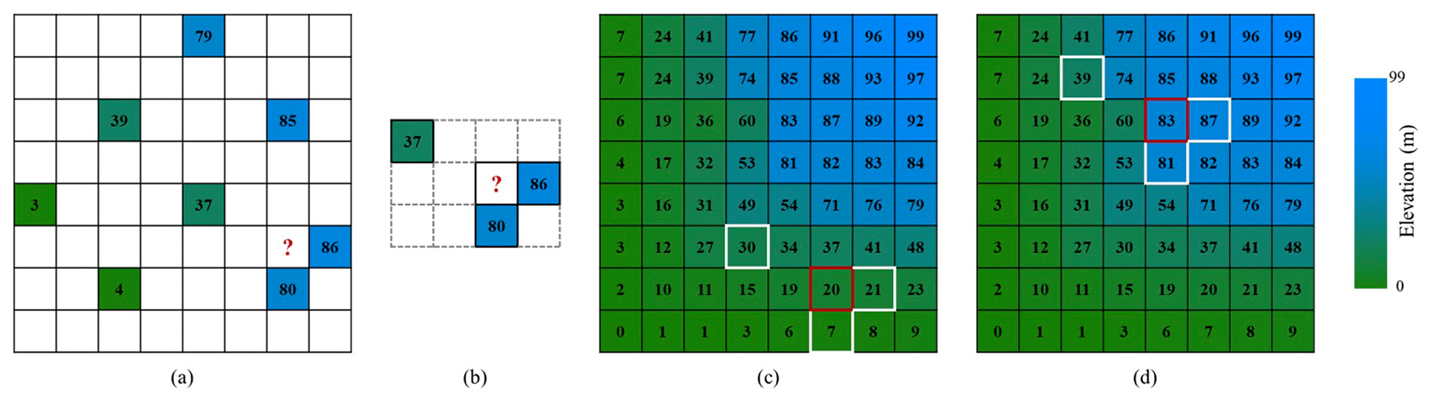
Figure 3Conceptual example of the DS point simulation. (a) Radar lines on the simulation grid; (b) three known points (values: 37, 80, 86) constitute a conditioning data pattern; (c) a mismatch pattern in TI; (d) a similar pattern in TI.
Based on the explanation above, there are three main key parameters within DS. (1) The first parameter is the number of conditioning points n. In a continuous simulation scenario, n≥30 is suggested to extract complex patterns from TI as well as the simulation grid (Bruna et al., 2019; Meerschman et al., 2013). (2) Then there is the distance threshold t. It is possible that there is no completely matching structure in the TI. Therefore, the algorithm accepts a training pattern whose distance with the conditioning pattern is lower than t. When many suitable patterns exist in TI, the first pattern found will be accepted. The value of t has a significant influence on the DS performance. A small value will improve modelling quality but may result in a significant computational cost. In most cases, t=0.1 is generally recognized as the upper bound (Meerschman et al., 2013; Zuo et al., 2020). (3) Lastly, there is the fraction of scanned TI f. Repeated morphological structures can be common in TI. With the aim of saving time, we can scan only a fraction of TI. For example, f=0.1 implies that the computer only inspects 10 % TI. According to the investigation conducted by Mariethoz and Caers (2014), a recommended value of f ranges from 0.1 to 0.5.
3.1.3 A metric space for training images
A metric space expresses the relationship between objects by using a distance function defining the similarity between any two objects. In metric spaces, we do not know the exact coordinates of objects but only how far objects are apart. Metric spaces are therefore useful in representing high-dimensional objects, such as training images. In this paper, we employ metric spaces for two purposes: (1) to visualize the difference between training images and (2) to estimate probabilities of training images to occur over some areas.
To define a meaningful distance between any two training images, we create a set of representative patterns for each training image. The TI morphological features are mainly concerned when creating the representative patterns. This requires first removing the effects of the original TI elevations. To do so, we rescale each TI to a range between 0 and 1 by min–max normalization (Han et al., 2012). Then, like other MPS approaches (Honarkhah and Caers, 2010; Strebelle, 2002), we extract all the spatial patterns from each TI using a fixed template. Next, we use agglomerative hierarchical clustering (Romary et al., 2015) to divide the spatial patterns of each TI into a finite number of groups. The number of groups is determined by a distance threshold between the clustered groups in agglomerative hierarchical clustering. As mentioned in Sect. 3.1.2, we set the distance threshold as 0.1 since it is commonly used to distinguish two patterns in DS (Meerschman et al., 2013). Therefore, a TI with more complex spatial patterns will have more clusters and thus more representative patterns. The medoid pattern of each group is taken as the representative pattern of the TI. Figure 4 shows a few representative patterns. The distance used in the clustering is the normalized Euclidean distance between the pixel-wise evaluations.

Figure 4Calculating the distance between any two training images (TIA and TIB) using modified Hausdorff distance. There are three key steps. (1) The first is to extract training patterns with a fixed template. (2) The representatives are selected by a hierarchical clustering method. In this example, the method found 16 important patterns from TIA, and 21 patterns are from TIB. The number of representatives is dependent on the complexity of morphology. (3) The third step is to calculate the modified Hausdorff distance between two pattern sets. The output distance becomes an indicator of similarity between two TIs.
After clustering and medoid selection, TIs can now be expressed by a set of representative patterns. We define the difference between any two training images as the difference between their sets of representative patterns. To do this, we use the modified Hausdorff distance (Dubuisson and Jain, 1994; Huttenlocher et al., 1993). This distance is commonly used to quantify the difference between shapes of high-dimensional objects. In detail, if we call the set of representative patterns for training image A as 𝒜 and for training image B as ℬ, then the modified Hausdorff distance is
where x𝒜 any one of the representative patterns in 𝒜, and yℬ is any pattern in ℬ. d is the Euclidean distance between any two representative patterns. |A| and |B| are respectively the sizes of 𝒜 and ℬ. In essence, the modified Hausdorff distance represents the maximum of expected minimum distances between the two TIs' representative patterns. Once a distance is defined, we can visualize the metric space in low-dimensional Cartesian space using multi-dimensional scaling or MDS (Scheidt et al., 2018). The main idea of MDS is to project objects from a high-dimensional space into a 2-D Cartesian space to visualize the similarity between all TIs. Figure 5 shows the projection of 166 training images in 2-D; each dot represents a TI. Similar training images map close to each other in the MDS scatterplot.
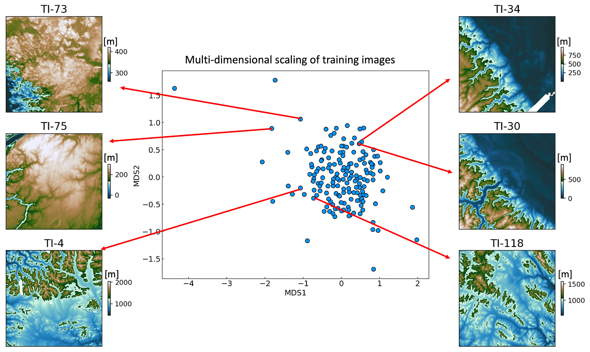
Figure 5Visualization of the metric space using multi-dimensional scaling (MDS) into a two-dimensional Cartesian space. Each dot on the plot represents a TI. It shows TIs with similar morphology are close in this metric space.
3.2 Illustration case and overview of the mapping strategy
To illustrate the proposed methodology, we focus on a small area of the ASE overlapping Pine Island Glacier (see Fig. 6). In this area, we observe a variety of radar line geometries and densities, as well as elevation changes. This smaller area is divided into four subareas. Strategies for such subdivision will be discussed later in the application to the entire domain. Direct sampling, by construction, avoids any artefact boundary between the radar line subareas, because the data template is not limited by subareas borders. With this strategy, two problems now need to be addressed. First, we need to find training images that are consistent with radar data within a selected subarea. There could be multiple such training images. Second, we need to model training image cross-correlation between different subareas. Training images of two adjacent subareas are not necessarily independent because of spatial correlations between the subareas. Our approach is to model the posterior TI distribution of each area through a probability aggregation problem.
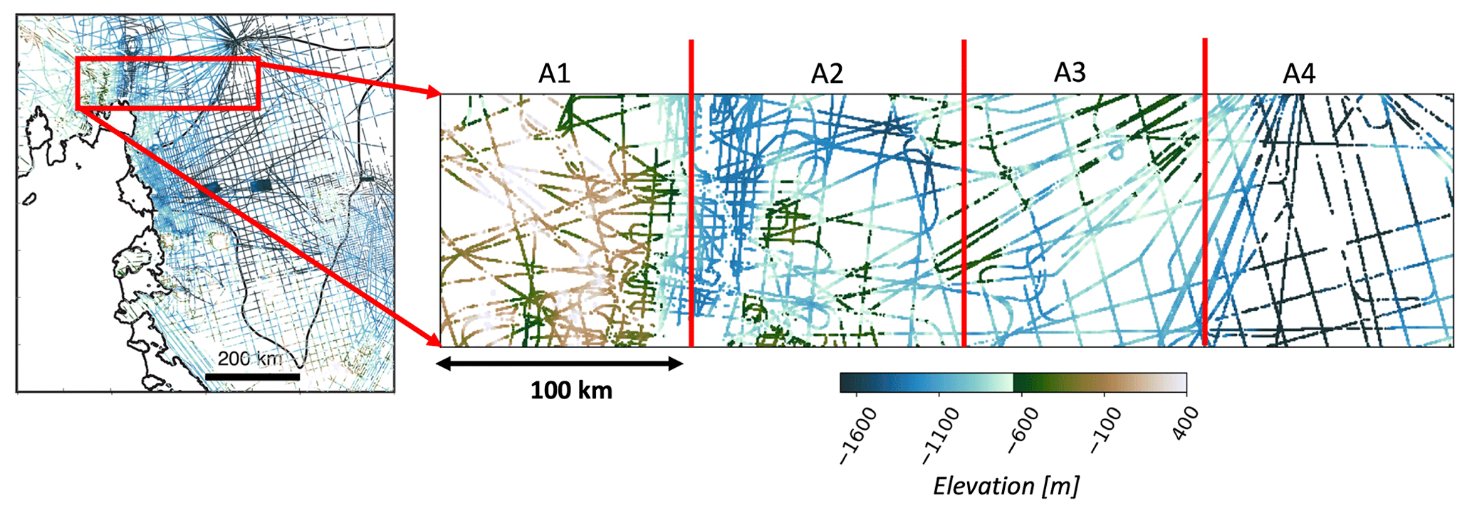
Figure 6A subset of the pine island glacier is used to illustrate the methodology. The red line divided four subareas: A1, A2, A3, and A4. The black coloured areas highlight line gaps of the selected subset.
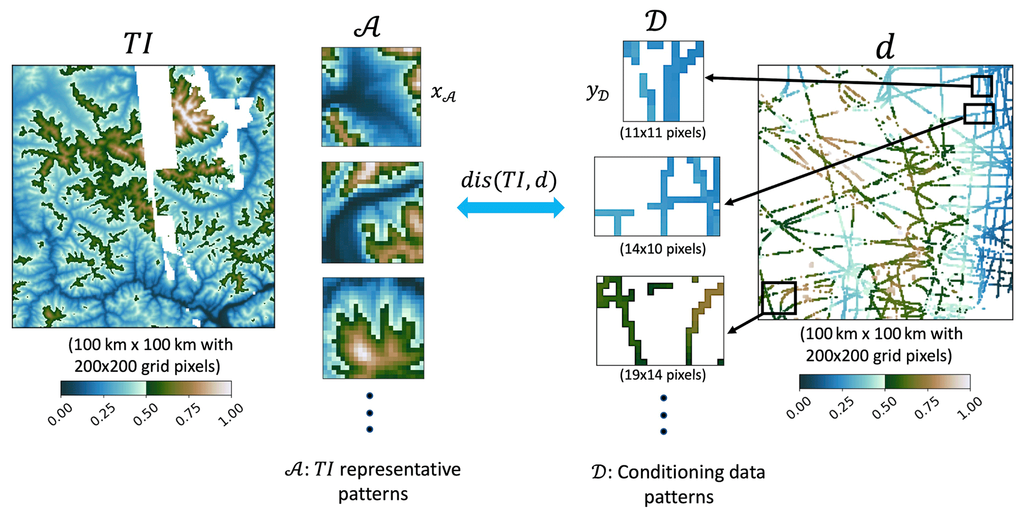
Figure 7Illustration of measuring the distance between training image and radar line data (d) in subarea A1. We first extract a group of radar data patterns D from the simulation grid with flexible-sized templates. Then the Hausdorff distances between the representative patterns A and radar patterns D are individually computed. Representative pattern xA has a fixed size of 23×23 pixels, while the size of conditioning data pattern yD varies.
3.3 Formulation of the problem through probability aggregation
Our goal is to estimate, for each area A1,…A4, the posterior distribution of training images, given the flight radar line data . This can be formulated as
TI(Ai) is a discrete random variable that has 166 possible outcomes (number of candidate TIs). To obtain the posterior distribution, we first estimate individual conditional probability ), then aggregate them into a single estimate for Eq. (2). We will use a simple aggregation model that uses log ratios (Allard et al., 2012), as follows:
Here, i and j are indices of the subarea, respectively. To aggregate these individual conditional probabilities, the log ratios can be summed relative to the prior:
Here, ri is the log ratio of in Eq. (2). r is the log ratio of the prior. The prior is a uniform distribution over all training images. Thus r is calculated as
Then, we can solve Eq. (4) for ri and invert the log ratio to get ).
However, in summing, we make a conditional independence assumption (Allard et al., 2012). Indeed, summing logarithms is equivalent to making products of the actual probabilities, which entails a form of conditional independence. Assuming conditional independence, when that assumption is untrue in reality, often results in overconfidence and too-small uncertainty. To mitigate this issue, we add an additional weight term wij:
Logically, we would like the weight to account for the correlation between data in different regions. For example, if data of region Ai are highly correlated with data in region Aj, then they are likely redundant with respect to the training image selection. Hence, we will make the weight wij function of the correlation structure between different subareas. In the next section, we will detail the subtasks ahead: (1) modelling and estimating ) and (2) calculating the weights wij.
3.4 Probability of training images given radar line data
3.4.1 Most probable set of training images
A direct estimate of ) is challenging because the line data are very high dimensional. For example, there are 7982 radar measurements in subarea A2. We turn this high-dimensional problem into a low-dimensional space as follows. Using the data in area Ai, we find those training images that constitute a set of most probable training images, i.e. those images closest to the radar lines in that area in terms of morphological similarities. We term this set as . Then given this set, we replace the radar line data with the most probable set:
To determine this set, we solve the following optimization problem:
where 𝕀TI is an indicator function which returns , a n-size subset of TI. , which is the total set of training images. We will explain how to determine the size n of via particle swarm optimization (see the Appendix). The distance (dis) in Eq. (8) measures the distance between the radar line data and any given training image. To calculate dis, we rely on the same modified Hausdorff distance approach as in Sect. 3.1.3:
𝒟 is now the set of patterns y𝒟 extracted from the radar lines. By pattern, we mean the radar line data are scanned within a given template. We use flexible-sized templates when scanning the radar lines over each subarea Ai. The template size varies in order to collect 40 neighbouring radar data points but with a maximum radius up to 15 pixels. 𝒜 is the set of TI representative patterns x𝒜, obtained in Sect. 3.1.3. Figure 7 provides an illustration of this idea.

Figure 8(a) The estimated set of most probable training images on MDS plots for each subarea (A1, A2, A3, A4). The red dots highlight the estimated . (b) Examples of displayed in the topographic modelling space.
We use a particle swarm optimization (PSO) to minimize the distance function (see the Appendix). As a heuristic optimization approach, PSO has its specific advantages in requiring less parameterization, easy implementation, and fast convergence with good accuracy (Rezaee Jordehi and Jasni, 2013; Sengupta et al., 2019). These characteristics make PSO a preferred optimizer for our initial training image selection. In conjunction with PSO, we employ the profile log-likelihood function to find the optimal size n of . A detailed explanation of the PSO algorithm and profile log-likelihood function implementations is provided in the Appendix. Figure 8 shows the selected in metric space for each subarea (A1, A2, A3, and A4). In this figure, we also plot examples of in the radar line map grid.
3.4.2 Kernel density estimation of )
We will use the optimal set of training images to infer ). We assume that TIs near the on the MDS plot tend to have similarly high probability of being assigned to the radar data subarea. This is because nearby TIs in the MDS metric space (see Fig. 5) show similar morphological patterns. We therefore consider a Gaussian kernel density estimation (KDE) to predict the probability of TI being assigned to a subarea Ai. The probability of each TI is estimated according to its distance with in the MDS plot (Fig. 5):
Here, is the kth selected TI using PSO. n is the size of the set . ) is modified Hausdorff distance between a TI and . K is the Gaussian kernel function (Eq. 11). The bandwidth h is the variance of the Gaussian kernel. We calculate the optimal bandwidth h by following Silverman's rule of thumb (Silverman, 1981). Figure 9 shows the KDE-estimated probability of each TI for subarea A1.

Figure 9(a) Estimated for subarea A1 in MDS space. The red dots are the , while blue points represent other TIs. (b) Kernel density smoothing assigns likelihoods (densities) to the total set of training images by using .
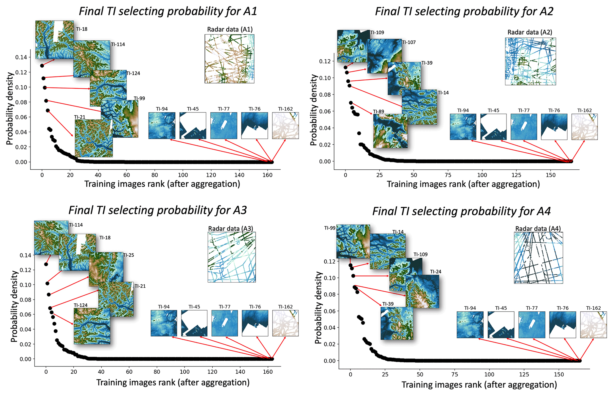
Figure 10Probability distribution of final aggregated TI probability in each radar line subarea.
3.5 Aggregation by weighting log ratios
Next, we aggregate the KDE-estimated probabilities by weighting the log ratios to obtain the posterior . The weights wij required in the log-ratio aggregation of Eq. (6) are used to quantify the spatial correlation between the radar line subareas. We use a variogram-based approach proposed by Fouedjio (2020) to measure spatial correlation between any two areas. In detail, the variogram dissimilarity is calculated as the sum of absolute values of all direct and cross variograms between the two subareas.
where dissim(Ai,Aj) is the dissimilarity between subareas Ai and Aj. According to Fouedjio (2020), (xi,xj) are the spatial centre locations of Ai and Aj, respectively. xl and are the radar data point locations in Ai and Aj. KE(⋅) is the Epanechnikov kernel function (Fouedjio, 2020). z(x) are the radar data measured values at location x. Using the calculated dissim(Ai,Aj), the weights wij are
With wij, we can aggregate the probability using the Eq. (4). Figure 10 shows the aggregated posterior probability of TIs for each subarea.
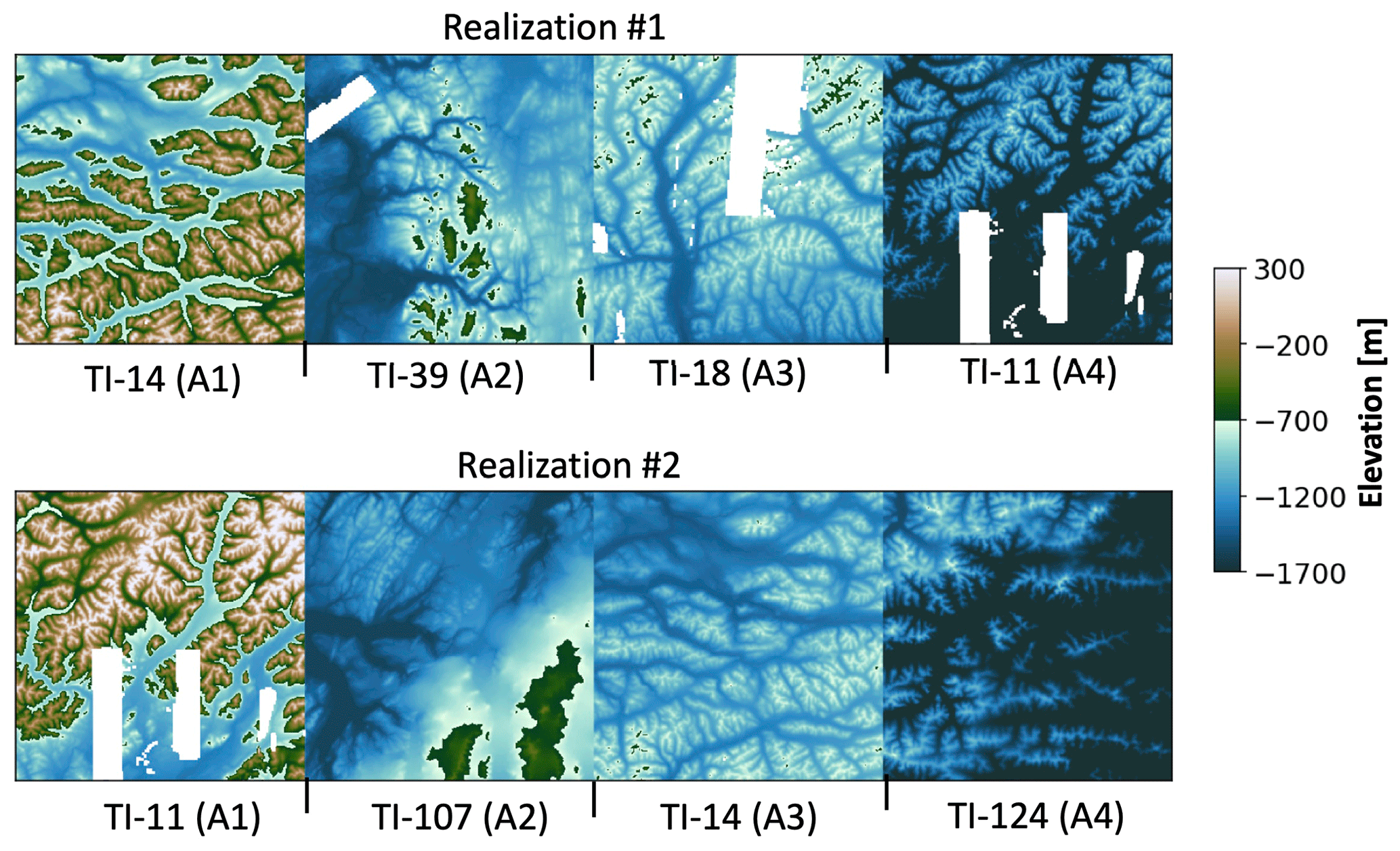
Figure 11Examples of sampled TIs from the posterior distributions corresponding to the subarea (A1, A2, A3, A4). The TIs are rescaled back to the local radar data range by inverting the min–max normalization.
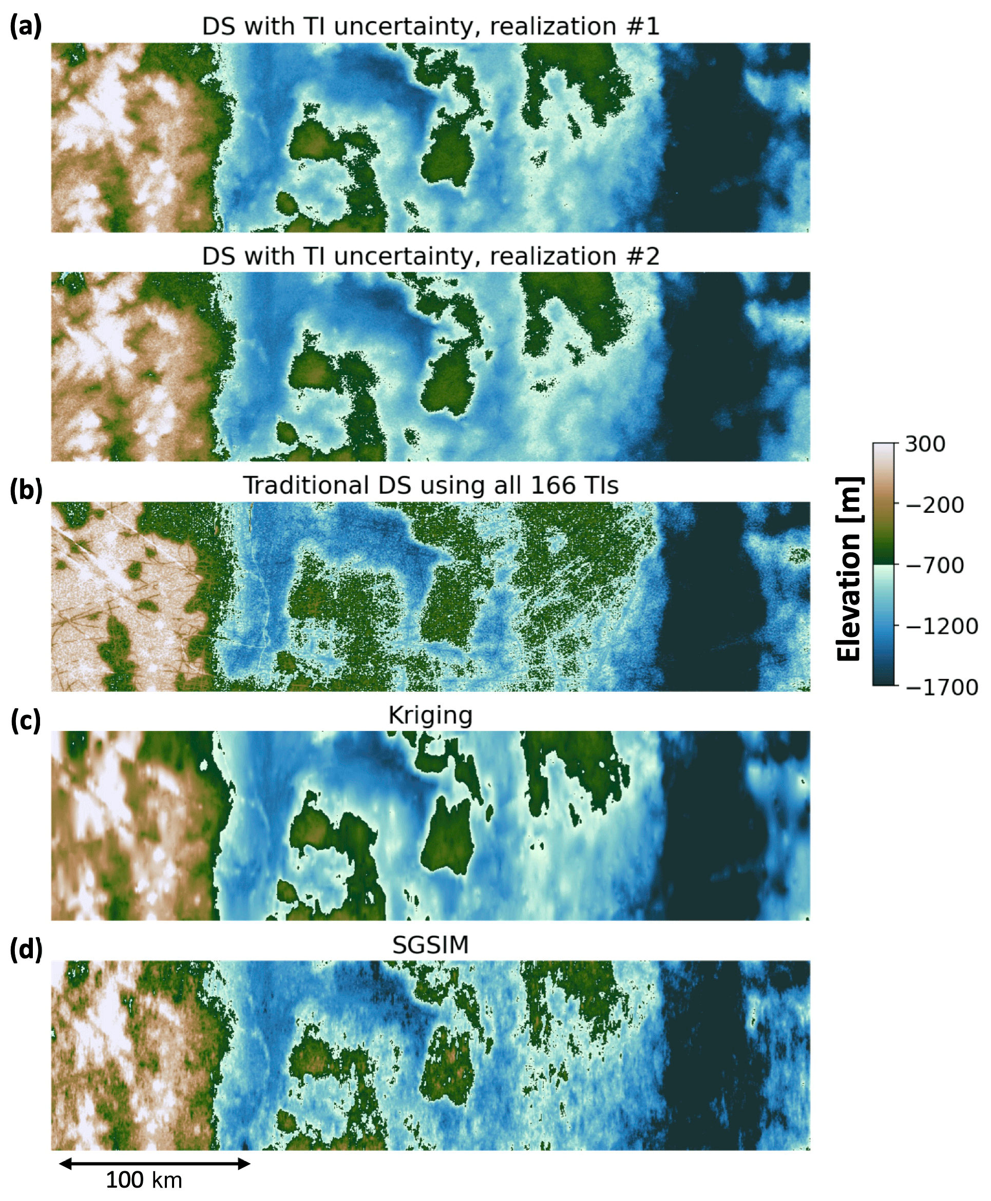
Figure 12(a) Two topographical model realizations from using our proposed DS with uncertain TI sampling to fill the radar line gaps. The model realization number corresponds to the TI realization number in Fig. 11. (b) Line gap filling by traditional DS using all the 166 TIs (without TI sampling). Panels (c) and (d) show line gap filling using kriging and SGSIM.
3.6 Direct sampling with uncertain TI sampling
Using the aggregated posterior TI probability ), we can now sample training images from the posterior distribution (Fig. 10) in each subarea. Figure 11 plots two realizations of sampled training images on the radar line map. We observe that the sampled topography TIs are different between the realizations. For example, the TIs sampled for A1 tend to have higher elevations and more mountain peaks than A2. A2 and A4 tend to have larger-scale low-elevation valleys, while the TIs in A1 and A3 data have more small-scale valleys. For each realization of training images, we run a DS simulation. Finally, multiple realizations of topographical models are generated, each with multiple realizations of TIs. Figure 12a shows two example realizations of the DS simulated results. We can observe large valleys in A2 and A4 areas, while A1 and A3 areas mainly have high elevation peaks. The non-stationarity of both simulated topography realizations also agreed well with their sampled TIs when compared to the TIs in Fig. 11.
3.7 Comparison with traditional MPS modelling and two-point geostatistical modelling
Our results are compared to the conventional MPS simulation without proposed TI sampling. Here, we use the same DS simulation parameters as our TI sampling approach, except that the training images are different. In the conventional test, we run the DS simulation by scanning all 166 TIs to fill the radar line gaps. Figure 12b shows one realization created by the conventional DS. It is obvious that the conventional approach results in a much noisier topographical model, and there are significant line artefacts that make the model unrealistic. To gain a detailed understanding, we take a cross section A–A′ across the trunk of Pine Island Glacier and plot the gap-filling result comparison in Fig. 13. We can observe that the DS without TI sampling creates more unrealistic elevation peaks and troughs. In particular, at the main channel of Pine Island Glacier (marked by the dashed box in Fig. 13) where dense radar data are available, unrealistic channels are simulated between the radar data observations. This suggests that, when using all the 166 TIs without proper sampling, the DS finds too-large a set of patterns of which many are incompatible with the sparse data. Our TI sampling approach avoids this problem by limiting the algorithm to a small number of most suitable TIs, thereby improving the result (see Fig. 12a). More importantly, avoiding the channel artefacts is critically important for modelling subglacial hydrological flow (see Sect. 4.2). In terms of running time, the conventional DS approach with 166 TIs took nearly 21 h to simulate one realization. By contrast, our TI sampling approach took less than 1 h. Our initial DS implementation tests are run on a PC with an Intel i9-11900 2.5 GHz processor and 32 GB of RAM.
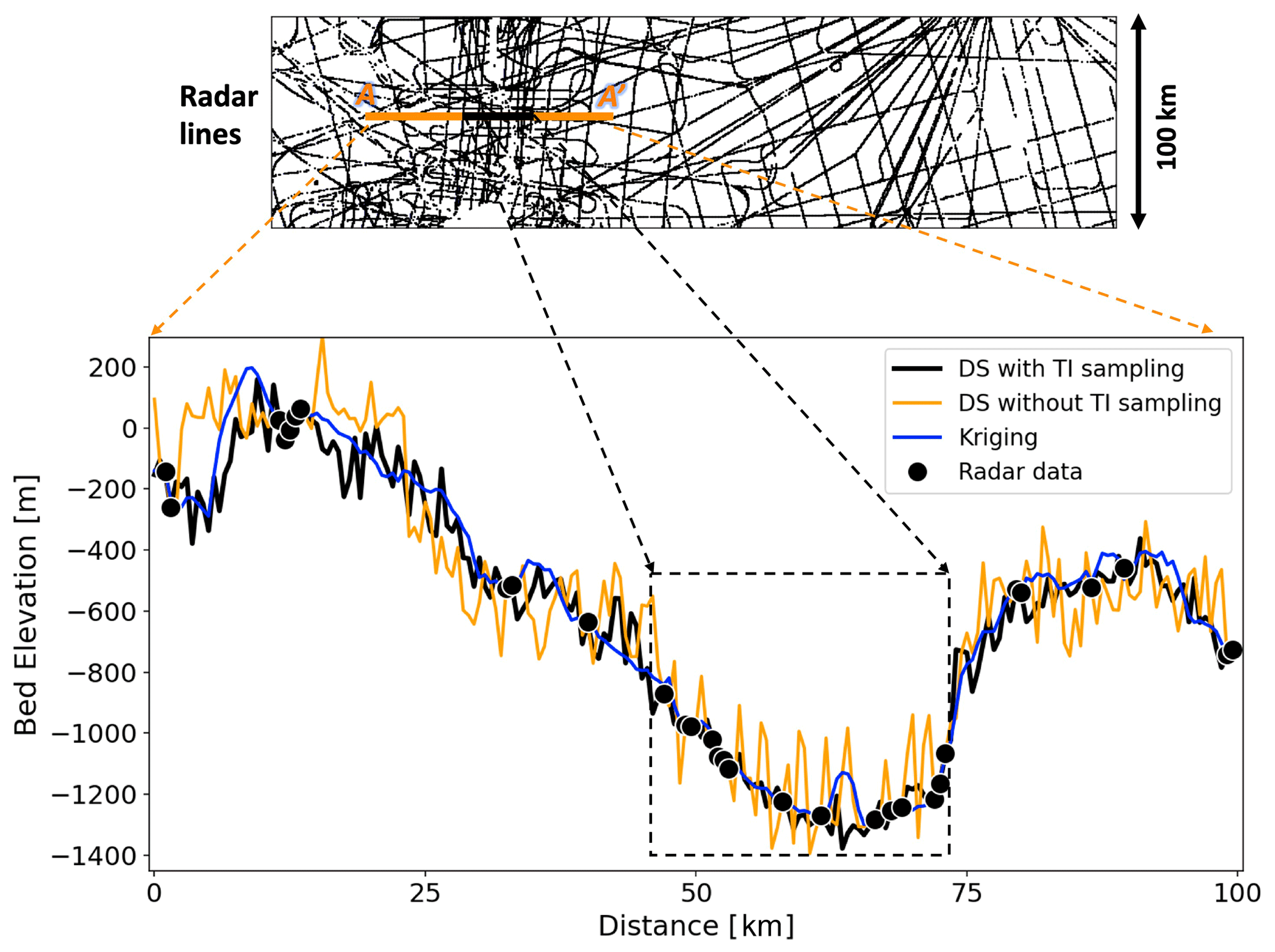
Figure 13Cross-section view of the modelled topography maps at line A–A′. The dashed black box shows main channel of Pine Island Glacier.

Figure 14Comparison of SGSIM and the proposed method of DS with uncertain TI sampling in a local sparse line area. Red ovals highlight the areas where SGSIM does not to simulate morphologically meaningful channels.
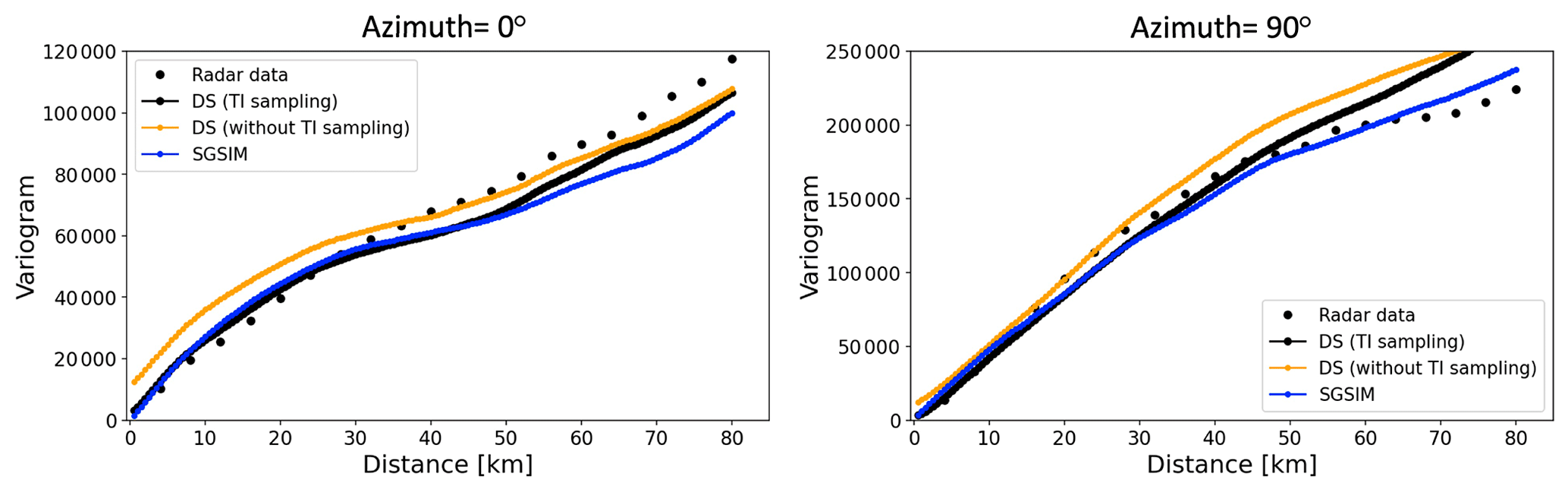

We further compare our approach with the two-point geostatistical modelling methods, kriging, and SGSIM (Fig. 12c and d). We observe that kriging produces the smoothest topographical model. The oversmoothed features are clear from the detailed cross section in Fig. 13. Besides, kriging is a deterministic modelling approach. It cannot generate multiple topographical models to quantify the spatial uncertainty. The SGSIM approach here uses local ordinary kriging; this way, non-stationarity is addressed by limiting the neighbourhood of spatial inference. As a spatial covariance-based approach, SGSIM is limited in its ability to capture complex morphological features, especially when the radar line data are very sparse. This limitation can be clearly observed in Fig. 14, where SGSIM does not produce morphologically meaningful channels in the area with sparse lines when comparing to our proposed approach. In Fig. 15, we further compare the empirical variograms from the modelled topographical maps using the three different approaches. It shows the DS using sampled TIs has reproduced the observed radar data variogram. The SGSIM maps also reproduce the variograms from the observed radar data, because they directly use the radar data variograms for modelling. However, the DS without TI sampling has a nugget (noise) effect. Overall, it shows the TI sampling approach performs the best in terms of improving the modelling speed, simulation quality, and capturing the spatial uncertainty. It is also important to note that there are other TI selection approaches. For example, Pérez et al. (2014) ranked TIs using high-order consistency with conditioning data, while Abdollahifard et al. (2019) used image contours to select compatible TIs. The unique contribution of our approach is that it quantifies posterior probabilities and uses a sampling method. In this sampling method, we may use different TIs for different realizations generated, as shown later in Fig. 17.
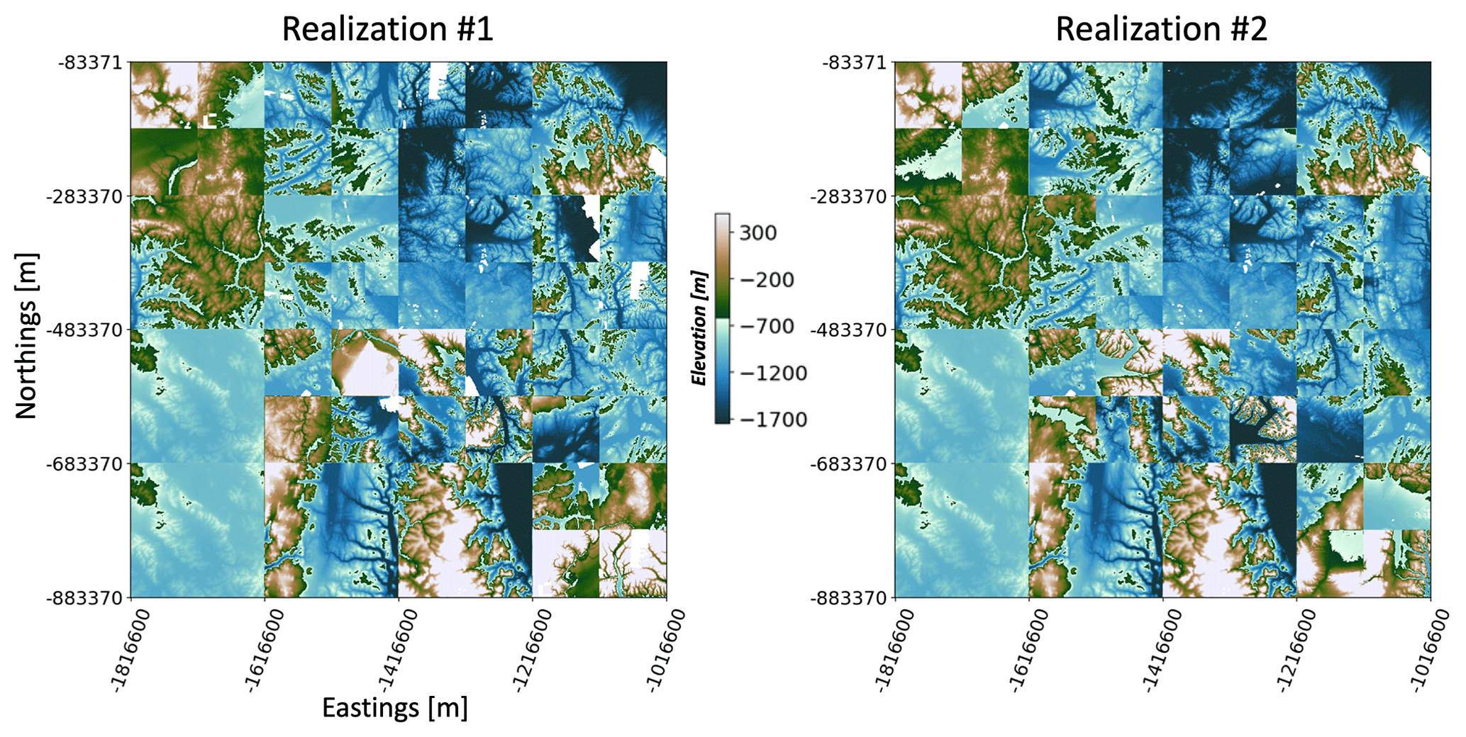
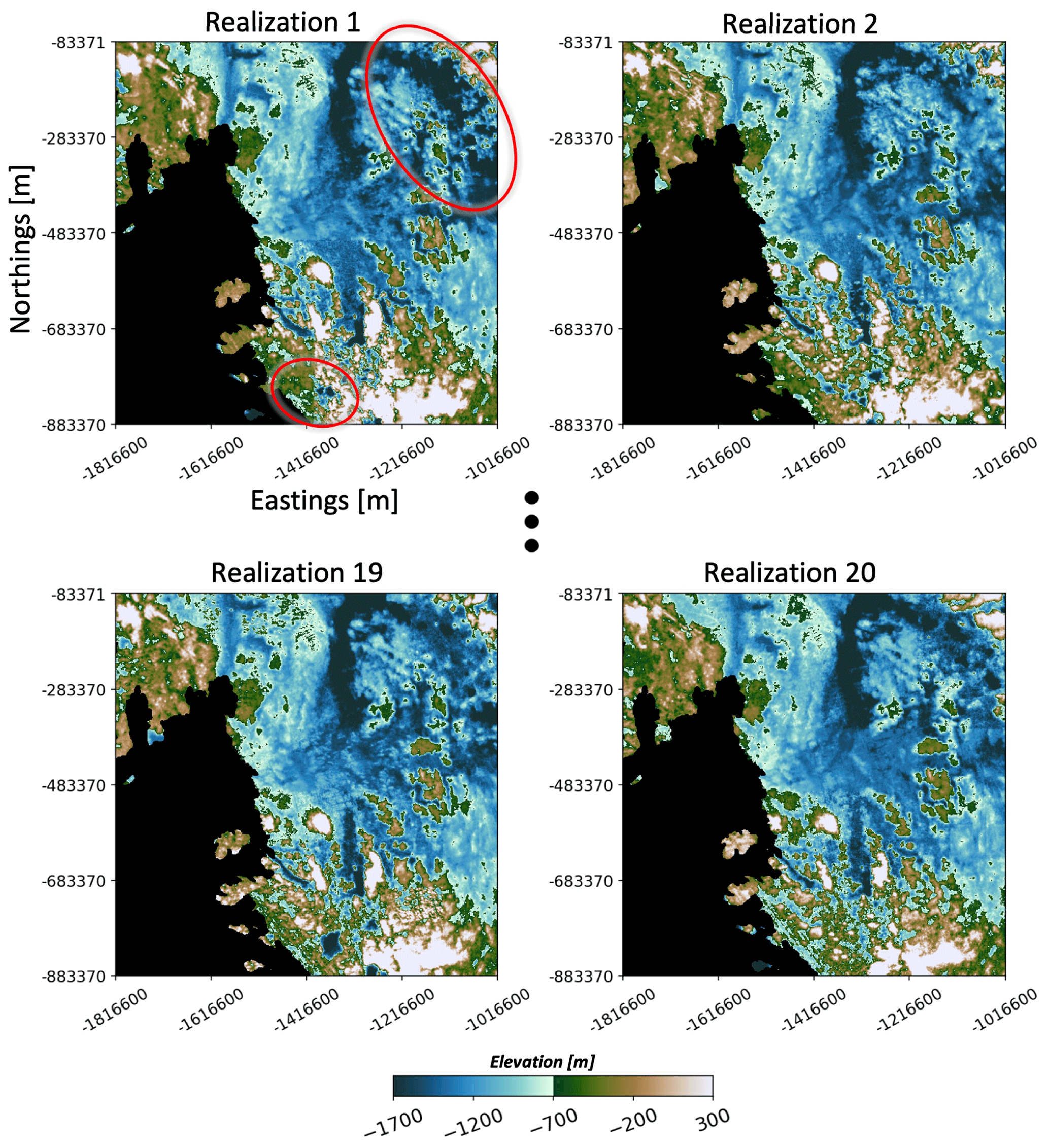
Figure 18Realizations of the ASE topography after filling the radar line gaps. The ovals highlight the areas with high spatial variations across the realizations. The black area is the non-study area with no radar data.
4.1 Training image sampling and DS simulation
We apply the proposed methodology to fill the radar line gaps of the entire ASE area to generate high-quality topography maps at a resolution of 500 m. To address the spatial non-stationarity and sample TIs, we first divide the whole ASE area into local subareas. We use the following recursive steps to divide the entire ASE into L subareas based on the line data density:
- Step 1.
Equally divide the ASE area into four quadrants in the shape of a square.
- Step 2.
For each subarea, if it has more than N radar data points, continue to divide it into four equally sized areas.
- Step 3.
Repeat step 2 until the number of data measurements is below the threshold number N. In this case, we set N=10 000 and divide ASE into a total of 56 subareas.
Figure 16 shows the final ASE subareas with the corresponding radar data density. Next, we calculate posterior TI probability for each subarea . We can then use the posterior probability to sample one single TI for each subarea. Figure 17 plots two realizations of the sampled TIs in the entire ASE space. For each TI realization, we run DS to fill the radar line gaps to generate high-resolution topography maps. To reflect the spatial uncertainty, 20 topography map realizations are simulated using 20 realizations of TI sets. The generated high-resolution bed topography is shown in Fig. 18.
4.2 Uncertainty in subglacial hydrological flow
We use the topographic realizations to investigate the sensitivity of subglacial water routing to topographic uncertainty. A water-routing model was applied to the 20 realizations generated from Sect. 4.1 to model the flow of water at the ice–bed interface. The direction of water flow can be determined by calculating hydraulic potential, ϕ, using the Shreve equation (Shreve, 1972):
where ρw is the density of water (1000 kg m−3), ρi is the density of ice (917 kg m−3), g is gravitational acceleration 9.8 m s−2), h is bed elevation, and H is ice thickness. The hydrological model was implemented using the Antarctic Mapping Tools (Greene et al., 2017) and the FLOWobj function and multiple flow direction (MFD) algorithm from the TopoToolbox package (Schwanghart and Scherler, 2014). These functions use the hydraulic potential gradient to compute flow accumulation, or the number of pixels that flow into another pixel. We use the “multi” setting, where downward flow in different directions is distributed based on a hydraulic gradient. We assume spatially uniform basal melt rates and that the subglacial pressure is equal to the ice overburden pressure. The results are compared to a hydrological model made using BedMachine topography (Morlighem et al., 2020), which was derived using the mass conservation inversion method.
The water-routing models vary across each realization (Fig. 19). In particular, the Thwaites Glacier tributaries flowing towards the grounding zone (the area where the ice meets the ocean and decouples from the bed) show significant differences across each realization. The average of the hydrological models across different realizations is different from the hydrological model made using the mass conservation topography, particularly in the main trunk of Thwaites Glacier (Fig. 19d and e). This demonstrates that deterministic DEMs cannot be used to sample the range of possible flow path locations, which could lead to the misinterpretation of hydrological conditions. In contrast, geostatistical simulation provides a framework for quantifying hydrological uncertainty with respect to topographic uncertainty.
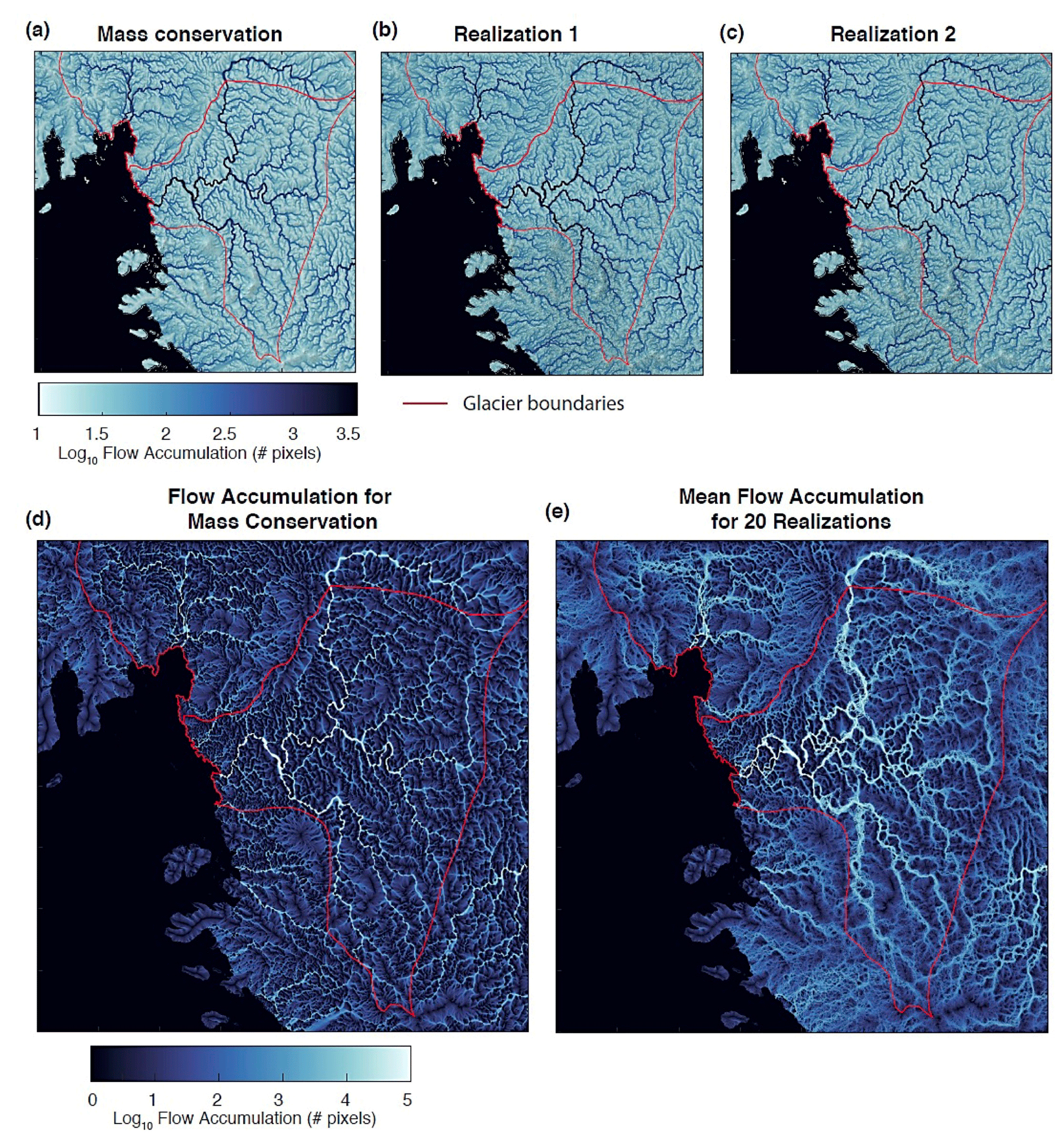
Figure 19(a) Subglacial water routing from mass conservation; (b, c) water routing using two topographic realizations from our DS simulation with TI sampling; (d) flow accumulation for mass conservation; (e) mean flow accumulation for 20 topographic realizations from our DS simulation.
Some of the modelled tributaries are located over a system of active subglacial lakes – lakes at the ice–bed interface that periodically drain and refill (Hoffman et al., 2020; Smith et al., 2017). These lakes are hypothesized to be hydrologically connected, with a drain and refill cycle that depends on the level of connectivity (Malczyk et al., 2020; Smith et al., 2017). Lake drainage events are sometimes associated with increases in ice velocity (Fricker et al., 2016; Stearns et al., 2008), making it important to characterize the connectivity of active lake systems. The topographic models created by the proposed method can be used to investigate the nature of hydrological drainage at Thwaites and highlight areas that require additional observational constraints.
We developed a non-stationary multiple-point geostatistical approach to fill large-scale geophysical data gaps and applied it to map high-resolution (500 m) subglacial topography of the Amundsen Sea Embayment in West Antarctica. The radar data gaps were filled using morphological features learned from high-resolution topographic training images. To reflect the geospatial uncertainty, we modelled multiple realizations of topography maps using 166 high-resolution training images from the Arctic and Antarctica. These training images represent the diversity of subglacial geologic settings. We have placed them in a publicly accessible repository for training subglacial topography models (see Data and code availability section). The TI repository can be further expanded in the future upon the acquisition of additional swath bathymetry and swath radar measurements.
Our major contribution was to show a probabilistic method to model posterior TI probabilities, then sample TIs to model the global non-stationarity in subglacial topography. This was achieved by probabilistically assigning non-stationary TIs from the provided repository to the local radar data. We used the collected 166 topographic training images as prior. The posterior distribution is calculated based on the modified Hausdorff distance between each TI and local radar data. To address the spatial correlation across the global area, we aggregate the TI probability between the local areas based on their spatial correlation. The aggregated posterior TI distribution then enabled us to sample training images. Finally, we ran DS to fill the radar line gaps. Multiple realizations of high-resolution topography maps were generated using multiple realizations of sampled training images. This non-stationary TI sampling framework avoids the use of auxiliary variables and arbitrary ad-hoc weighting. It has significantly improved the topography modelling quality from DS. It also dramatically reduced the DS running time from 21 to 1 h when given a large number of training images. Compared to the traditional deterministic interpolation (kriging) and two-point geostatistical simulation (SGSIM) approaches, our approach was shown to provide more realistic topographic maps for spatial uncertainty quantification, whilst retaining the spatial correlation measured by radar data.
We applied our proposed approach to fill the radar line gaps for the entire Amundsen Sea Embayment in West Antarctica. The improved modelling efficiency enabled us to simulate 20 realistic high-resolution topographic maps on a local PC. We then used the 20 topographic realizations to investigate the sensitivity of subglacial water routing to topographic uncertainty. The results reveal significant variabilities in the Thwaites Glacier tributaries across different realizations. These tributaries intersect a system of active subglacial lakes, which are hypothesized to be hydrologically connected and could have the potential to influence ice sheet velocity. The high hydrological uncertainty in this area highlights the need for additional measurement constraints. These findings demonstrate the utility of geostatistically simulating subglacial topography rather than performing deterministic interpolations. Our non-stationary MPS framework provides a path forward for implementing geostatistical simulations at continental scales.
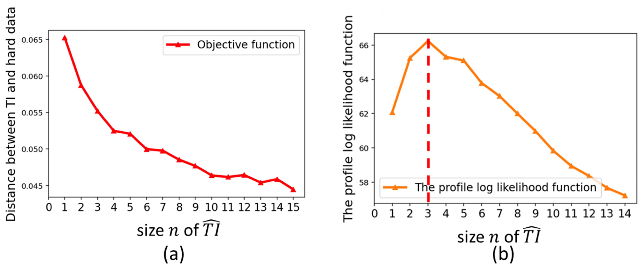
Figure A1(a) PSO minimum distance vs. the swarm size n. (b) Profile log likelihood of the curve in panel (a), suggesting the optimal number of training images is three.
We perform particle swarm optimization to minimize the distance function in Eq. (8). Following the PSO algorithm (Rezaee Jordehi and Jasni, 2013), we start with a random initialization of m selected TIs). Each individual TI selection is regarded as an individual particle (Pi). To find TIs that minimize the distance function, each particle will explore the whole TI space iteratively with a velocity Vi. The position (TI index) of Pi at time step t+1 is determined by its previous position Pi(t) and searching “velocity” Vi(t+1).
The velocity Vi(t+1) is determined by the particle's current logged best TI index and the best TI index for the whole swarm, as
where Vi(t) is the velocity from the previous time step. w is the “inertia weight” that controls the contribution of Vi(t) to Vi(t+1). A smaller w means less influence from the previous velocity and thus higher PSO exploration capability. Here, we set w as 0.8 according to the study by Han et al. (2010). r1 and r2 are two random numbers for a stochastic update of the velocity. They have a uniform distribution with the interval of [0,1]. c1 and c2 are the acceleration parameters that pull the particles towards and . are recommended for most optimization problems according to Ozcan and Mohan (1999). We adopt the recommended settings. The swarm size m also affects the PSO performance. So far, there are no exact rules for the selection of swarm size (Rezaee Jordehi and Jasni, 2013). Here, we use the size n of to determine the swarm size m. We create particles in the PSO population to enhance searching ability and running time.
Another important question is how to determine the optimal number n of . To specify n, we use a profile log-likelihood approach from Zhu and Ghodsi (2006) and Honarkhah and Caers (2010). Specifically, we expect that the distance between training images and radar line data will decrease as we visit more training images. The PSO optimized distance should decrease dramatically when the optimal n TIs is visited and then start flattening out. Hence, there will be an elbow point corresponding to the optimal number of TIs. Based on the study in Honarkhah and Caers (2010), the elbow is found by maximizing profile log likelihood. We find the optimal number of TIs using the following steps.
-
Run PSO to obtain the minimized distances disn with different size n, where .
-
For every n, we define two samples of and . Calculate the log likelihood ln(n) as
where μ1, μ2 are the means of φ1 and φ2, By contrast, σ2 is the common scale variance. σ1 and σ2 are the sample variances of φ1 and φ2.
-
Obtain the optimal (elbow) size based on the empirical maximum value of ln(n).
We use the illustration case area A1 as an example to show how to select . Figure A1a plots the PSO distance function between A1 radar lines and TIs with varying TI numbers. We can observe a fast drop of the distance at the beginning, and the distance then drops slowly after n=3. To find out the exact elbow, we calculate the log-likelihood values and plot them in Fig. A1b. Figure A1b clearly indicates that the optimal number of TIs is three.
The subglacial topography training image database is publicly available at https://doi.org/10.5281/zenodo.5083715 (MacKie et al., 2021b). The MPS modelling code and notebooks (MPS-BedMappingV1) used in this study are available on GitHub https://github.com/sdyinzhen/MPS-BedMappingV1 (last access: 4 September 2021) and archived at https://doi.org/10.5281/zenodo.5453360 (Yin et al., 2021).
ZY and CZ are co-first authors and contributed the main concepts and methodology development, conducted the technical applications, and drafted this paper.
EJM is the second author and prepared the project data, performed the hydrological modelling, contributed critical insights during the research developments, and drafted part of the paper.
JC is the PI of the research project and provided overall supervision and funding for this project, contributed major and critical ideas to the research development, and revised the manuscript.
The contact author has declared that neither they nor their co-authors have any competing interests.
Publisher's note: Copernicus Publications remains neutral with regard to jurisdictional claims in published maps and institutional affiliations.
This paper was edited by Alexander Robel and reviewed by John Goff, Wei Ji Leong, and one anonymous referee.
Abdollahifard, M. J., Baharvand, M., and Mariéthoz, G.: Efficient training image selection for multiple-point geostatistics via analysis of contours, Comput. Geosci., 128, 41–50, https://doi.org/10.1016/j.cageo.2019.04.004, 2019.
Allard, D., Comunian, A., and Renard, P.: Probability Aggregation Methods in Geoscience, Math. Geosci., 44, 545–581, https://doi.org/10.1007/s11004-012-9396-3, 2012.
Alley, R. B., Holschuh, N., MacAyeal, D. R., Parizek, B. R., Zoet, L., Riverman, K., Muto, A., Christianson, K., Clyne, E., Anandakrishnan, S., Stevens, N. and Collaboration, G.: Bedforms of Thwaites Glacier, West Antarctica: Character and Origin, J. Geophys. Res.-Earth Surf., 126, e2021JF006339, https://doi.org/10.1029/2021JF006339, 2021.
Almeida, A. S. and Journel, A. G.: Joint simulation of multiple variables with a Markov-type coregionalization model, Math. Geol., 26, 565–588, https://doi.org/10.1007/BF02089242, 1994.
Arndt, J. E., Schenke, H. W., Jakobsson, M., Nitsche, F. O., Buys, G., Goleby, B., Rebesco, M., Bohoyo, F., Hong, J., Black, J., Greku, R., Udintsev, G., Barrios, F., Reynoso-Peralta, W., Taisei, M., and Wigley, R.: The International Bathymetric Chart of the Southern Ocean (IBCSO) Version 1.0 – A new bathymetric compilation covering circum-Antarctic waters, Geophys. Res. Lett., 40, 3111–3117, https://doi.org/10.1002/grl.50413, 2013.
Bingham, R. G. and Siegert, M. J.: Quantifying subglacial bed roughness in Antarctica: implications for ice-sheet dynamics and history, Quaternary Sci. Rev., 28, 223–236, https://doi.org/10.1016/j.quascirev.2008.10.014, 2009.
Bingham, R. G., Vaughan, D. G., King, E. C., Davies, D., Cornford, S. L., Smith, A. M., Arthern, R. J., Brisbourne, A. M., De Rydt, J., Graham, A. G. C., Spagnolo, M., Marsh, O. J., and Shean, D. E.: Diverse landscapes beneath Pine Island Glacier influence ice flow, Nat. Commun., 8, 1618, https://doi.org/10.1038/s41467-017-01597-y, 2017.
Blankenship, D. D., Morse, D. L., Finn, C. A., Bell, R. E., Peters, M. E., Kempf, S. D., Hodge, S. M., Studinger, M., Behrendt, J. C., and Brozena, J. M.: Geologic Controls on the Initiation of Rapid Basal Motion for West Antarctic Ice Streams: A Geophysical Perspective Including New Airborne Radar Sounding and Laser Altimetry Results, The West Antarctic Ice Sheet: Behavior and Environment, 105–121, https://doi.org/10.1029/AR077p0105, 2001.
Bruna, P.-O., Straubhaar, J., Prabhakaran, R., Bertotti, G., Bisdom, K., Mariethoz, G., and Meda, M.: A new methodology to train fracture network simulation using multiple-point statistics, Solid Earth, 10, 537–559, https://doi.org/10.5194/se-10-537-2019, 2019.
Chugunova, T. L. and Hu, L. Y.: Multiple-Point Simulations Constrained by Continuous Auxiliary Data, Math. Geosci., 40, 133–146, 10.1007/s11004-007-9142-4, 2008.
Clarke, G. K. C., Berthier, E., Schoof, C. G., and Jarosch, A. H.: Neural Networks Applied to Estimating Subglacial Topography and Glacier Volume, J. Climate, 22, 2146–2160, https://doi.org/10.1175/2008JCLI2572.1, 2009.
De Fleurian, B., Werder, M. A., Beyer, S., Brinkerhoff, D. J., Delaney, I. A. N., Dow, C. F., Downs, J., Gagliardini, O., Hoffman, M. J., Hooke, R. L., Seguinot, J. and Sommers, A. N.: SHMIP The subglacial hydrology model intercomparison Project, J. Glaciol., 64, 897–916, https://doi.org/10.1017/jog.2018.78, 2018.
Deutsch, C. V. and Journel, A. G.: GSLIB Geostatistical Software Library and User’s Guide, 2nd Edn., Oxford University Press, pp 369, ISBN 0195100158, 1998.
Dubuisson, M. and Jain, A. K.: A modified Hausdorff distance for object matching, in: Proceedings of 12th International Conference on Pattern Recognition, Jerusalem, Israel, Abstract no. 4985725, vol. 1, 566–568, https://doi.org/10.1109/ICPR.1994.576361, 9–13 October 1994.
Farinotti, D., Brinkerhoff, D. J., Clarke, G. K. C., Fürst, J. J., Frey, H., Gantayat, P., Gillet-Chaulet, F., Girard, C., Huss, M., Leclercq, P. W., Linsbauer, A., Machguth, H., Martin, C., Maussion, F., Morlighem, M., Mosbeux, C., Pandit, A., Portmann, A., Rabatel, A., Ramsankaran, R., Reerink, T. J., Sanchez, O., Stentoft, P. A., Singh Kumari, S., van Pelt, W. J. J., Anderson, B., Benham, T., Binder, D., Dowdeswell, J. A., Fischer, A., Helfricht, K., Kutuzov, S., Lavrentiev, I., McNabb, R., Gudmundsson, G. H., Li, H., and Andreassen, L. M.: How accurate are estimates of glacier ice thickness? Results from ITMIX, the Ice Thickness Models Intercomparison eXperiment, The Cryosphere, 11, 949–970, https://doi.org/10.5194/tc-11-949-2017, 2017.
Fouedjio, F.: Clustering of multivariate geostatistical data, WIREs Comput. Stat., 12, e1510, https://doi.org/10.1002/wics.1510, 2020.
Fretwell, P., Pritchard, H. D., Vaughan, D. G., Bamber, J. L., Barrand, N. E., Bell, R., Bianchi, C., Bingham, R. G., Blankenship, D. D., Casassa, G., Catania, G., Callens, D., Conway, H., Cook, A. J., Corr, H. F. J., Damaske, D., Damm, V., Ferraccioli, F., Forsberg, R., Fujita, S., Gim, Y., Gogineni, P., Griggs, J. A., Hindmarsh, R. C. A., Holmlund, P., Holt, J. W., Jacobel, R. W., Jenkins, A., Jokat, W., Jordan, T., King, E. C., Kohler, J., Krabill, W., Riger-Kusk, M., Langley, K. A., Leitchenkov, G., Leuschen, C., Luyendyk, B. P., Matsuoka, K., Mouginot, J., Nitsche, F. O., Nogi, Y., Nost, O. A., Popov, S. V., Rignot, E., Rippin, D. M., Rivera, A., Roberts, J., Ross, N., Siegert, M. J., Smith, A. M., Steinhage, D., Studinger, M., Sun, B., Tinto, B. K., Welch, B. C., Wilson, D., Young, D. A., Xiangbin, C., and Zirizzotti, A.: Bedmap2: improved ice bed, surface and thickness datasets for Antarctica, The Cryosphere, 7, 375–393, https://doi.org/10.5194/tc-7-375-2013, 2013.
Fricker, H. A., Siegfried, M. R., Carter, S. P. and Scambos, T. A.: A decade of progress in observing and modelling Antarctic subglacial water systems, Philos. T. R. Soc. A, 374, 20140294, https://doi.org/10.1098/rsta.2014.0294, 2016.
Goff, J. A., Powell, E. M., Young, D. A., and Blankenship, D. D.: Conditional simulation of Thwaites Glacier (Antarctica) bed topography for flow models: Incorporating inhomogeneous statistics and channelized morphology, J. Glaciol., 60, 635–646, https://doi.org/10.3189/2014JoG13J200, 2014.
Gogineni, P.: CReSIS radar depth sounder data, Center for Remote Sensing of Ice Sheets, Lawrence, KS, https://data.cresis.ku. edu/ (last access: 10 December 2021), 2012.
Graham, F. S., Roberts, J. L., Galton-Fenzi, B. K., Young, D., Blankenship, D. and Siegert, M. J.: A high-resolution synthetic bed elevation grid of the Antarctic continent, Earth Syst. Sci. Data, 9, 267–279, https://doi.org/10.5194/essd-9-267-2017, 2017.
Gravey, M. and Mariethoz, G.: QuickSampling v1.0: a robust and simplified pixel-based multiple-point simulation approach, Geosci. Model Dev., 13, 2611–2630, https://doi.org/10.5194/gmd-13-2611-2020, 2020.
Greene, C. A., Gwyther, D. E., and Blankenship, D. D.: Antarctic Mapping Tools for Matlab, Comput. Geosci., 104, 151–157, https://doi.org/10.1016/j.cageo.2016.08.003, 2017.
Han, J., Kamber, M., and Pei, J.: 3 – Data Preprocessing, in: The Morgan Kaufmann Series in Data Management Systems, edited by: Han, J., Kamber, M., and J. B. T.-D. M. Third E. Pei, Morgan Kaufmann, Boston, 83–124, 2012.
Han, W., Yang, P., Ren, H., and Sun, J.: Comparison study of several kinds of inertia weights for PSO, in: 2010 IEEE International Conference on Progress in Informatics and Computing, Shanghai, China, Abstract no. 11747156m vol. 1, 280–284, https://doi.org/10.1109/PIC.2010.5687447, 10–12 December 2010.
Herzfeld, U. C., Eriksson, M. G., and Holmlund, P.: On the influence of kriging parameters on the cartographic output – A study in mapping subglacial topography, Math. Geol., 25, 881–900, https://doi.org/10.1007/BF00891049, 1993.
Hoffimann, J., Scheidt, C., Barfod, A., and Caers, J.: Stochastic simulation by image quilting of process-based geological models, Comput. Geosci., 106, 18–32, https://doi.org/10.1016/j.cageo.2017.05.012, 2017.
Hoffimann, J., Bufe, A., and Caers, J.: Morphodynamic Analysis and Statistical Synthesis of Geomorphic Data: Application to a Flume Experiment, J. Geophys. Res.-Earth, 124, 2561–2578, https://doi.org/10.1029/2019JF005245, 2019.
Hoffman, A. O., Christianson, K., Shapero, D., Smith, B. E., and Joughin, I.: Brief communication: Heterogenous thinning and subglacial lake activity on Thwaites Glacier, West Antarctica, The Cryosphere, 14, 4603–4609, https://doi.org/10.5194/tc-14-4603-2020, 2020.
Holschuh, N., Christianson, K., Paden, J., Alley, R. B., and Anandakrishnan, S.: Linking postglacial landscapes to glacier dynamics using swath radar at Thwaites Glacier, Antarctica, Geology, 48, 268–272, https://doi.org/10.1130/G46772.1, 2020.
Holt, J. W., Blankenship, D. D., Morse, D. L., Young, D. A., Peters, M. E., Kempf, S. D., Richter, T. G., Vaughan, D. G., and Corr, H. F. J.: New boundary conditions for the West Antarctic Ice Sheet: Subglacial topography of the Thwaites and Smith glacier catchments, Geophys. Res. Lett., 33, L09502, https://doi.org/10.1029/2005GL025561, 2006.
Honarkhah, M. and Caers, J.: Stochastic Simulation of Patterns Using Distance-Based Pattern Modeling, Math. Geosci., 42, 487–517, https://doi.org/10.1007/s11004-010-9276-7, 2010.
Honarkhah, M. and Caers, J.: Direct Pattern-Based Simulation of Non-stationary Geostatistical Models, Math. Geosci., 44, 651–672, https://doi.org/10.1007/s11004-012-9413-6, 2012.
Howat, I. M., Porter, C., Smith, B. E., Noh, M.-J., and Morin, P.: The Reference Elevation Model of Antarctica, The Cryosphere, 13, 665–674, https://doi.org/10.5194/tc-13-665-2019, 2019.
Huss, M. and Farinotti, D.: Distributed ice thickness and volume of all glaciers around the globe, J. Geophys. Res.-Earth, 117, F04010, https://doi.org/10.1029/2012JF002523, 2012.
Huttenlocher, D. P., Klanderman, G. A., and Rucklidge, W. J.: Comparing images using the Hausdorff distance, IEEE T. Pattern Anal., 15, 850–863, https://doi.org/10.1109/34.232073, 1993.
Joughin, I., Smith, B. E., and Medley, B.: Marine Ice Sheet Collapse Potentially Under Way for the Thwaites Glacier Basin, West Antarctica, Science, 344, 735–738, https://doi.org/10.1126/science.1249055, 2014.
Journel, A. and Zhang, T.: The Necessity of a Multiple-Point Prior Model, Math. Geol., 38, 591–610, https://doi.org/10.1007/s11004-006-9031-2, 2006.
King, E. C., Hindmarsh, R. C. A., and Stokes, C. R.: Formation of mega-scale glacial lineations observed beneath a West Antarctic ice stream, Nat. Geosci., 2, 585–588, https://doi.org/10.1038/ngeo581, 2009.
Laloy, E., Hérault, R., Jacques, D., and Linde, N.: Training-Image Based Geostatistical Inversion Using a Spatial Generative Adversarial Neural Network, Water Resour. Res., 54, 381–406, https://doi.org/10.1002/2017WR022148, 2018.
Le clec'h, S., Quiquet, A., Charbit, S., Dumas, C., Kageyama, M., and Ritz, C.: A rapidly converging initialisation method to simulate the present-day Greenland ice sheet using the GRISLI ice sheet model (version 1.3), Geosci. Model Dev., 12, 2481–2499, https://doi.org/10.5194/gmd-12-2481-2019, 2019.
Lythe, M. B., and Vaughan, D. G.: BEDMAP: A new ice thickness and subglacial topographic model of Antarctica, J. Geophys. Res., 106, 11335–11351, https://doi.org/10.1029/2000JB900449, 2001.
MacKie, E. J., Schroeder, D. M., Caers, J., Siegfried, M. R., and Scheidt, C.: Antarctic Topographic Realizations and Geostatistical Modeling Used to Map Subglacial Lakes, J. Geophys. Res.-Earth, 125, e2019JF005420, https://doi.org/10.1029/2019JF005420, 2020.
MacKie, E. J., Schroeder, D. M., Zuo, C., Yin, Z., and Caers, J.: Stochastic modeling of subglacial topography exposes uncertainty in water routing at Jakobshavn Glacier, J. Glaciol., 67, 75–83, https://doi.org/10.1017/jog.2020.84, 2021a.
MacKie, E., Yin, Z., Zuo, C., and Caers, J.: Subglacial Topography Training Image Database, Zenodo [data set], https://doi.org/10.5281/zenodo.5083715, 2021b.
Malczyk, G., Gourmelen, N., Goldberg, D., Wuite, J., and Nagler, T.: Repeat Subglacial Lake Drainage and Filling Beneath Thwaites Glacier, Geophys. Res. Lett., 47, e2020GL089658, https://doi.org/10.1029/2020GL089658, 2020.
Margold, M., Stokes, C. R., and Clark, C. D.: Ice streams in the Laurentide Ice Sheet: Identification, characteristics and comparison to modern ice sheets, Earth-Sci. Rev., 143, 117–146, https://doi.org/10.1016/j.earscirev.2015.01.011, 2015.
Mariethoz, G.: When Should We Use Multiple-Point Geostatistics? BT – Handbook of Mathematical Geosciences: Fifty Years of IAMG, edited by: Daya Sagar, B. S., Cheng, Q., and Agterberg, F., Springer International Publishing, Cham, 645–653, 2018.
Mariethoz, G. and Renard, P.: Reconstruction of Incomplete Data Sets or Images Using Direct Sampling, Math. Geosci., 42, 245–268, https://doi.org/10.1007/s11004-010-9270-0, 2010.
Mariethoz, G., Renard, P., and Straubhaar, J.: The Direct Sampling method to perform multiple-point geostatistical simulations, Water Resour. Res., 46, W11536, https://doi.org/10.1029/2008WR007621, 2010.
Mariethoz, G., McCabe, M. F., and Renard, P.: Spatiotemporal reconstruction of gaps in multivariate fields using the direct sampling approach, Water Resour. Res., 48, W10507, https://doi.org/10.1029/2012WR012115, 2012.
Mariethoz, P. G. and Caers, J.: Multiple-point Geostatistics: Stochastic Modeling with Training Images, Wiley, 376 pp., ISBN: 978-1-118-66293-9, 2014.
Matheron, G.: Principles of geostatistics, Econ. Geol., 58, 1246–1266, https://doi.org/10.2113/gsecongeo.58.8.1246, 1963.
Meerschman, E., Pirot, G., Mariethoz, G., Straubhaar, J., Van Meirvenne, M., and Renard, P.: A practical guide to performing multiple-point statistical simulations with the Direct Sampling algorithm, Comput. Geosci., 52, 307–324, https://doi.org/10.1016/j.cageo.2012.09.019, 2013.
Mo, S., Zabaras, N., Shi, X., and Wu, J.: Integration of Adversarial Autoencoders With Residual Dense Convolutional Networks for Estimation of Non-Gaussian Hydraulic Conductivities, Water Resour. Res., 56, e2019WR026082, https://doi.org/10.1029/2019WR026082, 2020.
Morlighem, M., Williams, C. N., Rignot, E., An, L., Arndt, J. E., Bamber, J. L., Catania, G., Chauché, N., Dowdeswell, J. A., Dorschel, B., Fenty, I., Hogan, K., Howat, I., Hubbard, A., Jakobsson, M., Jordan, T. M., Kjeldsen, K. K., Millan, R., Mayer, L., Mouginot, J., Noël, B. P. Y., O'Cofaigh, C., Palmer, S., Rysgaard, S., Seroussi, H., Siegert, M. J., Slabon, P., Straneo, F., van den Broeke, M. R., Weinrebe, W., Wood, M., and Zinglersen, K. B.: BedMachine v3: Complete Bed Topography and Ocean Bathymetry Mapping of Greenland From Multibeam Echo Sounding Combined With Mass Conservation, Geophys. Res. Lett., 44, 11051–11061, https://doi.org/10.1002/2017GL074954, 2017.
Morlighem, M., Rignot, E., Binder, T., Blankenship, D., Drews, R., Eagles, G., Eisen, O., Ferraccioli, F., Forsberg, R., Fretwell, P., Goel, V., Greenbaum, J. S., Gudmundsson, H., Guo, J., Helm, V., Hofstede, C., Howat, I., Humbert, A., Jokat, W., Karlsson, N. B., Lee, W. S., Matsuoka, K., Millan, R., Mouginot, J., Paden, J., Pattyn, F., Roberts, J., Rosier, S., Ruppel, A., Seroussi, H., Smith, E. C., Steinhage, D., Sun, B., Broeke, M. R. van den, Ommen, T. D. van, Wessem, M. van, and Young, D. A.: Deep glacial troughs and stabilizing ridges unveiled beneath the margins of the Antarctic ice sheet, Nat. Geosci., 13, 132–137, https://doi.org/10.1038/s41561-019-0510-8, 2020.
Neven, A., Dall'Alba, V., Juda, P., Straubhaar, J., and Renard, P.: Ice volume and basal topography estimation using geostatistical methods and ground-penetrating radar measurements: application to the Tsanfleuron and Scex Rouge glaciers, Swiss Alps, The Cryosphere, 15, 5169–5186, https://doi.org/10.5194/tc-15-5169-2021, 2021.
Oriani, F., Straubhaar, J., Renard, P., and Mariethoz, G.: Simulation of rainfall time series from different climatic regions using the direct sampling technique, Hydrol. Earth Syst. Sci., 18, 3015–3031, https://doi.org/10.5194/hess-18-3015-2014, 2014.
Ozcan, E. and Mohan, C. K.: Particle swarm optimization: surfing the waves, in: Proceedings of the 1999 Congress on Evolutionary Computation-CEC99 (Cat. No. 99TH8406), vol. 3, 1939–1944, 1999.
Pérez, C., Mariethoz, G., and Ortiz, J. M.: Verifying the high-order consistency of training images with data for multiple-point geostatistics, Comput. Geosci., 70, 190–205, https://doi.org/10.1016/j.cageo.2014.06.001, 2014.
Pirot, G., Straubhaar, J., and Renard, P.: Simulation of braided river elevation model time series with multiple-point statistics, Geomorphology, 214, 148–156, https://doi.org/10.1016/j.geomorph.2014.01.022, 2014.
Pirot, G., Straubhaar, J., and Renard, P.: A pseudo genetic model of coarse braided-river deposits, Water Resour. Res., 51, 9595–9611, https://doi.org/10.1002/2015WR017078, 2015.
Porter, C., Morin, P., Howat, I., Noh, M.-J., Bates, B., Peterman, K., Keesey, S., Schlenk, M., Gardiner, J., Tomko, K., Willis, M., Kelleher, C., Cloutier, M., Husby, E., Foga, S., Nakamura, H., Platson, M., Wethington Jr., M., Williamson, C., Bauer, G., Enos, J., Arnold, G., Kramer, W., Becker, P., Doshi, A., D'Souza, C., Cummens, P., Laurier, F., and Bojesen, M.: ArcticDEM, https://doi.org/10.7910/DVN/OHHUKH, 2018.
Pyrcz, M. J. and White, C. D.: Uncertainty in reservoir modeling, Interpretation, 3, SQ7–SQ19, https://doi.org/10.1190/INT-2014-0126.1, 2015.
Rezaee Jordehi, A. and Jasni, J.: Parameter selection in particle swarm optimisation: a survey, J. Exp. Theor. Artif. In., 25, 527–542, https://doi.org/10.1080/0952813X.2013.782348, 2013.
Rignot, E., Mouginot, J., Scheuchl, B., van den Broeke, M., van Wessem, M. J., and Morlighem, M.: Four decades of Antarctic Ice Sheet mass balance from 1979–2017, P. Natl. Acad. Sci. USA, 116, 1095–1103, https://doi.org/10.1073/pnas.1812883116, 2019.
Rippin, D. M., Bingham, R. G., Jordan, T. A., Wright, A. P., Ross, N., Corr, H. F. J., Ferraccioli, F., Le Brocq, A. M., Rose, K. C., and Siegert, M. J.: Basal roughness of the Institute and Möller Ice Streams, West Antarctica: Process determination and landscape interpretation, Geomorphology, 214, 139–147, https://doi.org/10.1016/j.geomorph.2014.01.021, 2014.
Romary, T., Ors, F., Rivoirard, J., and Deraisme, J.: Unsupervised classification of multivariate geostatistical data: Two algorithms, Comput. Geosci., 85, 96–103, https://doi.org/10.1016/j.cageo.2015.05.019, 2015.
Scheidt, C., Li, L., and Caers, J.: Quantifying Uncertainty in Subsurface Systems, Wiley, 63–66, ISBN: 978-1-119-32583-3, 2018.
Schlegel, N.-J., Seroussi, H., Schodlok, M. P., Larour, E. Y., Boening, C., Limonadi, D., Watkins, M. M., Morlighem, M., and van den Broeke, M. R.: Exploration of Antarctic Ice Sheet 100-year contribution to sea level rise and associated model uncertainties using the ISSM framework, The Cryosphere, 12, 3511–3534, https://doi.org/10.5194/tc-12-3511-2018, 2018.
Schmidt, A. M. and O'Hagan, A.: Bayesian inference for non-stationary spatial covariance structure via spatial deformations, J. R. Stat. Soc. Ser. B-Met., 65, 743–758, https://doi.org/10.1111/1467-9868.00413, 2003.
Schwanghart, W. and Scherler, D.: Short Communication: TopoToolbox 2 – MATLAB-based software for topographic analysis and modeling in Earth surface sciences, Earth Surf. Dynam., 2, 1–7, https://doi.org/10.5194/esurf-2-1-2014, 2014.
Sengupta, S., Basak, S. and Peters, R. A.: Particle Swarm Optimization: A Survey of Historical and Recent Developments with Hybridization Perspectives, Mach. Learn. Knowl. Extr., 1, 157–191, https://doi.org/10.3390/make1010010, 2019.
Seroussi, H., Nakayama, Y., Larour, E., Menemenlis, D., Morlighem, M., Rignot, E., and Khazendar, A.: Continued retreat of Thwaites Glacier, West Antarctica, controlled by bed topography and ocean circulation, Geophys. Res. Lett., 44, 6191–6199, https://doi.org/10.1002/2017GL072910, 2017.
Shreve, R. L.: Movement of Water in Glaciers, J. Glaciol., 11, 205–214, https://doi.org/10.3189/S002214300002219X, 1972.
Siegert, M. J., Ross, N., and Le Brocq, A. M.: Recent advances in understanding Antarctic subglacial lakes and hydrology, Philos. T. R. Soc. A, 374, 20140306, https://doi.org/10.1098/rsta.2014.0306, 2016.
Silverman, B. W.: Using Kernel Density Estimates to Investigate Multimodality, J. R. Stat. Soc. Ser. B-Met., 43, 97–99, https://doi.org/10.1111/j.2517-6161.1981.tb01155.x, 1981.
Smith, B. E., Gourmelen, N., Huth, A., and Joughin, I.: Connected subglacial lake drainage beneath Thwaites Glacier, West Antarctica, The Cryosphere, 11, 451–467, https://doi.org/10.5194/tc-11-451-2017, 2017.
Sommers, A., Rajaram, H., and Morlighem, M.: SHAKTI: Subglacial Hydrology and Kinetic, Transient Interactions v1.0, Geosci. Model Dev., 11, 2955–2974, https://doi.org/10.5194/gmd-11-2955-2018, 2018.
Spagnolo, M., Bartholomaus, T. C., Clark, C. D., Stokes, C. R., Atkinson, N., Dowdeswell, J. A., Ely, J. C., Graham, A. G. C., Hogan, K. A., King, E. C., Larter, R. D., Livingstone, S. J., and Pritchard, H. D.: The periodic topography of ice stream beds: Insights from the Fourier spectra of mega-scale glacial lineations, J. Geophys. Res.-Earth, 122, 1355–1373, https://doi.org/10.1002/2016JF004154, 2017.
Srivastava, M. R.: The Origins of the Multiple-Point Statistics (MPS) Algorithm BT – Handbook of Mathematical Geosciences: Fifty Years of IAMG, edited by: Daya Sagar, B. S., Cheng, Q., and Agterberg, F., Springer International Publishing, Cham, 655–672, 2018.
Stearns, L. A., Smith, B. E., and Hamilton, G. S.: Increased flow speed on a large East Antarctic outlet glacier caused by subglacial floods, Nat. Geosci., 1, 827–831, https://doi.org/10.1038/ngeo356, 2008.
Strebelle, S.: Conditional Simulation of Complex Geological Structures Using Multiple-Point Statistics, Math. Geol., 34, 1–21, https://doi.org/10.1023/A:1014009426274, 2002.
Strebelle, S. B. and Journel, A. G.: Reservoir Modeling Using Multiple-Point Statistics, SPE Annu. Tech. Conf. Exhib., 11, SPE-71324-MS, https://doi.org/10.2118/71324-MS, 2001.
Tahmasebi, P.: Multiple Point Statistics: A Review BT – Handbook of Mathematical Geosciences: Fifty Years of IAMG, edited by: Daya Sagar, B. S., Cheng, Q., and Agterberg, F., Springer International Publishing, Cham, 613–643, 2018.
Vaughan, D. G., Corr, H. F. J., Ferraccioli, F., Frearson, N., O'Hare, A., Mach, D., Holt, J. W., Blankenship, D. D., Morse, D. L., and Young, D. A.: New boundary conditions for the West Antarctic ice sheet: Subglacial topography beneath Pine Island Glacier, Geophys. Res. Lett., 33, https://doi.org/10.1029/2005GL025588, 2006.
Williams, C. K. I. and Rasmussen, C. E.: Gaussian processes for regression, in: Advances in Neural Information Processing Systems 8, edited by: Touretzky, D. S., Mozer, M. C., and Hasselmo, M. E., MIT, ISBN: 0262201070, 1996
Wu, J., Boucher, A., and Zhang, T.: A SGeMS code for pattern simulation of continuous and categorical variables: FILTERSIM, Comput. Geosci., 34, 1863–1876, https://doi.org/10.1016/j.cageo.2007.08.008, 2008.
Yin, G., Mariethoz, G., and McCabe, M. F.: Gap-Filling of Landsat 7 Imagery Using the Direct Sampling Method, Remote Sens., 9, 12, https://doi.org/10.3390/rs9010012, 2017.
Young, D. A., Schroeder, D. M., Blankenship, D. D., Kempf, S. D., and Quartini, E.: The distribution of basal water between Antarctic subglacial lakes from radar sounding, Philos. T. R. Soc. A-Math., 374, 20140297, https://doi.org/10.1098/rsta.2014.0297, 2016.
Zakeri, F. and Mariethoz, G.: A review of geostatistical simulation models applied to satellite remote sensing: Methods and applications, Remote Sens. Environ., 259, 112381, https://doi.org/10.1016/j.rse.2021.112381, 2021.
Zhou, H., Gómez-Hernández, J. J., and Li, L.: Inverse methods in hydrogeology: Evolution and recent trends, Adv. Water Resour., 63, 22–37, https://doi.org/10.1016/J.ADVWATRES.2013.10.014, 2014.
Zuo, C., Yin, Z., Pan, Z., MacKie, E. J., and Caers, J.: A Tree-Based Direct Sampling Method for Stochastic Surface and Subsurface Hydrological Modeling, Water Resour. Res., 56, e2019WR026130, https://doi.org/10.1029/2019WR026130, 2020.