An automatic lake-model application using near-real-time data forcing: development of an operational forecast workflow (COASTLINES) for Lake Erie

For enhanced public safety and water resource management, a three-dimensional operational lake hydrodynamic forecasting system, COASTLINES (Canadian cOASTal and Lake forecastINg modEl System), was developed. The modeling system is built upon the three-dimensional Aquatic Ecosystem Model (AEM3D) model, with predictive simulation capabilities developed and tested for a large lake (i.e., Lake Erie). The open-access workflow derives model forcing, code execution, post-processing, and web-based visualization of the model outputs, including water level elevations and temperatures, in near-real time. COASTLINES also generates 240 h predictions using atmospheric forcing from 15 and 25 km horizontal-resolution operational meteorological products from the Environment Canada Global Deterministic Forecast System (GDPS). Simulated water levels were validated against observations from six gauge stations, with model error increasing with forecast horizon. Satellite images and lake buoys were used to validate forecast lake surface temperature and the water column thermal stratification. The forecast lake surface temperature is as accurate as hindcasts, with a root-mean-square deviation <2 ^∘C. COASTLINES predicted storm surges and up-/downwelling events that are important for coastal flooding and drinking water/fishery management, respectively. Model forecasts are available in real time at https://coastlines.engineering.queensu.ca/ (last access: January 2022​​​​​​​). This study provides an example of the successful development of an operational forecasting workflow, entirely driven by open-access data, that may be easily adapted to simulate aquatic systems or to drive other computational models, as required for management and public safety.

1 Introduction

Lakes hold a large proportion of the global surface freshwater, which supports biodiversity and supplies water resources for drinking, transportation, and recreation. However, anthropogenic stressors are causing significant changes in the properties of lakes, such as rapid warming of surface water (O'Reilly et al., 2015), large seasonal water level fluctuations (Gronewold and Rood, 2019), increased frequency of extreme events (Saber et al., 2020), and severe water quality issues such as oxygen depletion (Rowe et al., 2019; Scavia et al., 2014) and harmful algal blooms (Brookes and Carey, 2011; Watson et al., 2016). Effort has focused on investigating the long-term responses of physical processes in lakes to climate change (O'Reilly et al., 2015; Woolway and Merchant, 2019; Jabbari et al., 2021), but improving lake monitoring and developing short-term forecast models to predict the occurrence of extreme events is also necessary (Woolway et al., 2020). The biogeochemical cycles in lakes are complex and often regulated by physical forcing; therefore, the first step to model and forecast water quality issues, such as harmful algal blooms (Paerl and Paul, 2012; O'Neil et al., 2012) and hypoxia (Rao et al., 2008, 2014), is the development of accurate hydrodynamic models.

Over the past several decades, many computer models have been applied to hindcast (running models forced with and validated against historically collected data) lake hydrodynamics to aid management. These range from one-dimensional (1-D) models such as the Dynamics Reservoir Simulation Model (DYRESM) (Antenucci and Imerito, 2000), Simstrat (Gaudard et al., 2017), and GLM (Hipsey et al., 2014) to three-dimensional (3-D) models such as Delft3D (Lesser et al., 2004), FVCOM (Chen et al., 2012; Rowe et al., 2019), and the Estuary and Lake Computer Model (ELCOM) (Hodges et al., 2000). Several of these hydrodynamic models may be coupled to biogeochemical models to allow for prediction of water quality. In the case of hindcast applications, the complex and time-consuming setup and calibration procedure of these models can result in a significant time lag (months to years) between when a project is initiated and when the model results are communicated to stakeholders. This delay severely limits the utility of computational models for policy and management decision making. For better application of these powerful computational tools, the ability to obtain rapid monitoring and simulation forecasts should be established.

In addition to the significant effort required to setup and calibrate models, other hurdles exist, such as data-sharing agreements between the agencies collecting forcing/validation data and those running the models. For example, the US National Oceanic and Atmospheric Administration (NOAA) Great Lakes Coastal Forecasting System (GLCFS) (Chu et al., 2011; Anderson et al., 2018) is a comparatively large-budget multi-institutional (NOAA-GLERL and U. Michigan-CIGLR) project that predicts water levels, temperature profiles, currents, and wave heights over a 120 h timeframe in the five Laurentian Great Lakes and connecting channels, using FVCOM on a 3-D unstructured grid with 30–2000 m horizontal resolution. Similarly, http://meteolakes.ch (last access: December 2021)​​​​​​​ (Baracchini et al., 2020b) applies Delft3D for short-term 3-D forecasts (4.5 d) of four Swiss lakes and http://simstrat.eawag.ch (last access: December 2021​​​​​​​) (Gaudard et al., 2019) applies Simstrat for near-real-time 1-D simulation of 54 Swiss​​​​​​​ lakes. These latter applications employ a data-sharing agreement between Swiss Federal Institute of Aquatic Science and Technology (EAWAG), École Polytechnique Fédérale de Lausanne (EPFL) and MeteoSwiss.

Due to the present online proliferation of near-real-time lake observation data (e.g., National Data Buoy Center (NDBC; https://www.ndbc.noaa.gov/, last access: December 2021​​​​​​​); Great Lakes Observation System (GLOS; http://www.glos.us/, last access: December 2021)) and high-resolution meteorological forecasts (e.g., Global Deterministic Prediction System, GDPS; http://dd.weather.gc.ca/model_gem_global/, last access: December 2021; High Resolution Rapid Refresh, HRRR; http://rapidrefresh.noaa.gov/hrrr/, last access: December 2021), the data-sharing agreements and managed data transfer protocols are no longer required. When coupled with recent dramatic improvements in workflow efficiency (e.g., Gaudard et al., 2019; Baracchini et al., 2020b), near-real-time inclusion of forcing from meteorological forecasts allows for the development of specific simulations tailored to meet diverse lake-management needs (e.g., prediction of coastal flooding, spill modeling, fish habitat, beach closures, and optimization of treatment or source water monitoring strategies).

In the present study, we developed and tested the COASTLINES (Canadian cOASTal and Lake forecastINg modEl System; http://coastlines.engineering.queensu.ca/, last access: December 2021) lake-model application workflow that rapidly accesses near-real-time online data (weather forecasts, water level, and temperature observations) for automated model forcing, execution, and validation. Hydrodynamic forecasts are automatically post-processed and posted on a web platform. We provide an overview of the COASTLINES system, including model implementation for Lake Erie (Sect. 2: data and methods) and the accuracy of COASTLINES in forecasting water levels and temperature fields over timescales of 24 and 240 h (Sect. 3: results). In the discussion (Sect. 4), the predictive ability of COASTLINES for decision making is showcased through prediction of hydrodynamic events associated with fish kills, hypoxia near a drinking water intake, and coastal flooding from a storm surge. We also discuss the relative advantages of COASTLINES in comparison to other model products, including bias and uncertainty.

2 Data and methods

2.1 Study site

Lake Erie is the shallowest lake of the Great Lakes with a mean depth of 19 m. Lake-wide hydrodynamics predominantly exhibits free surface and current oscillations from the 14 h barotropic seiche (Hamblin, 1987; Boegman et al., 2001). The lake morphometry consists of distinct, yet interconnected western, central, and eastern basins (Fig. 1), each with its own water quality concerns: the 11 m deep western basin is typically well mixed and has frequent harmful algae blooms related to climate-driven meteorological forcing (Michalak et al., 2013). The ephemeral stratification in late summer (Loewen et al., 2007) regulates vertical biogeochemical fluxes (Boegman et al., 2008). The 20 m deep central basin is prone to large-scale hypolimnetic hypoxia (Scavia et al., 2014). Hydrodynamics are governed by an internal Poincaré wave (Bouffard et al., 2012; Valipour et al., 2015) and a bowl-shaped depression of the summer thermocline, which influence the oxygen budget (Beletsky et al., 2012; Bouffard et al., 2014). The 65 m deep eastern basin has nearshore water quality concerns from Cladophora (Higgins et al., 2006) and ecosystem engineering by dreissenid mussels (Hecky et al., 2004). Hydrodynamics of this region are controlled by the coastal internal Kelvin wave (Valipour et al., 2019).

Figure 1 Map of Lake Erie showing the bathymetric depths and observation sites. The bathymetric map is at the resolution of the 500 m grid applied in the model. The western, central, and eastern basins are labeled as WB, CB, and EB, respectively. Blue circles indicate lake buoys and black squares indicate water level gauges.

2.2 Model description

COASTLINES applies the three-dimensional Aquatic Ecosystem Model (AEM3D, version 1.1.1, HydroNumerics Pty Ltd.). This model solves the unsteady 3-D Reynolds-averaged Navier–Stokes equations for incompressible flow employing the Boussinesq and hydrostatic approximations. Momentum advection is based on the Euler–Lagrange method with a conjugate-gradient solution for the free-surface height (Casulli and Cheng, 1992) and a conservative ULTIMATE QUICKEST discretization scheme for advection of scalars (Leonard, 1991). AEM3D is a parallel version of the commonly applied ELCOM (Hodges et al., 2000). ELCOM has been applied to Lake Erie to simulate currents and seasonal circulation (León et al., 2005), the internal Poincaré (Valipour et al., 2015) and Kelvin waves (Valipour et al., 2019), ice cover (Oveisy et al., 2012), and the response of the thermal structure, in Lake Erie, to air temperature and wind speed changes (Liu et al., 2014). ELCOM has been coupled with the biogeochemical the Computational Aquatic Ecosystem Dynamics Model (CAEDYM) to simulate Lake Erie phytoplankton and nutrients (León et al., 2011), and the response of hypoxia (Bocaniov and Scavia, 2016) and algae blooms (Scavia et al., 2016) to nutrient load reductions. Recent applications of AEM3D include a study of the water level in Lake Arrowhead, California (Saber et al., 2020), ice cover in Lake Constance (Caramatti et al., 2019), and pollutant transport in Lake St. Clair (Madani et al., 2020).

2.3 Model setup and meteorological forcing variables

To adequately resolve the coastal boundary layer (∼ 3 km width (Rao and Murthy, 2001)) and basin-scale internal waves (Poincaré (16.8 h) and Kelvin waves), the bathymetry of Lake Erie (https://www.ngdc.noaa.gov/mgg/greatlakes/erie.html, last access: January 2021​​​​​​​) was discretized into a 500 m × 500 m horizontal grid, which is ∼ 10 % of the internal Rossby radius (Schwab and Beletsky, 1998). The lake was discretized into 45 vertical layers, with fine resolution (0.5 m) through the surface layer, metalimnion and bottom of the central basin, and coarse layers (5 m) through the hypolimnion of the deeper eastern basin to the maximum depth of 64 m.

The model was “cold started” on 8 April 2020​​​​​​​ (day of year 99) with an initial temperature field spatially interpolated from observed water temperatures at stations 45142 and MHRO1, a time when spring turnover causes thermal stratification to be minimal. The model time step is dt=300 s to satisfy the Courant–Friedrichs–Lewy (CFL) of $\sqrt{\mathrm{2}}$ condition for internal waves (Hodges et al., 2000).

The model is forced by the surface meteorology (wind speed, wind direction, air temperature, shortwave solar radiation, relative humidity, air pressure, and net longwave radiation), with net longwave radiation being computed internally within AEM3D from cloud cover and the modeled surface temperature. In order to address the spatial variability of meteorological conditions across the lake, the computational domain was forced with meteorological data on horizontal grids at 15 km (https://dd.weather.gc.ca/model_gem_global/15km/, last access: January 2022) and 25 km (https://dd.weather.gc.ca/model_gem_global/25km/, last access: October 2021) resolution using meteorological forecasts from the Environment and Climate Change Canada Global Deterministic Forecast System (GDPS). This resulted in 31 and 23 meteorological sections for the 15 and 25 km models, respectively. Wind speed, wind direction, air temperature, relative humidity, air pressure, dew point, and cloud cover are direct outputs from GDPS, with solar radiation calculated based on dew point and air pressure (Meyers and Dale, 1983; Appendix C in Gaudard et al., 2019). The meteorological forecast has an output time step of 3 h and a forecast length of 240 h. The GRIB2 meteorological data were retrieved with the “urllib” library in Python and formatted into AEM3D input files using the nctoolbox in MATLAB.

In this pilot application, the Lake Erie inflows and outflows, which roughly balance, are neglected; however, evaporation and precipitation are accounted for in the water balance. Over short timescales (<10 d), the contributions from evaporation and precipitation to water level change are minor, with water level oscillations resulting from storm surges and surface seiches (Trebitz, 2006).

2.4 Observations, implementation, and model validation

The water levels and temperatures simulated by COASTLINES were validated using both in situ and satellite observations. Near-real-time water level data were used from six stations along the Canadian coastline, which reported hourly observations (Bar Point, Kingsville, Erieau, Port Stanley, Port Dover, and Port Colborne; Fig. 1; Table 1), retrieved from Fisheries and Oceans Canada (https://marees.gc.ca/eng/find/zone/44, last access: January 2022). The data are parsed using the “BeautifulSoup” library in Python and saved as .csv files to be read with MATLAB for model validation. The observations showed higher fluctuations in the western (Bar Point and Kingsville) and eastern (Port Dover and Port Colborne) basins (Fig. 1). Thus, we quantify the water level forecast capability and uncertainty in terms of the root-mean-square deviation (RMSD) and relative error (RE):

$$\begin{array}{}\text{(1)}& {\displaystyle }\mathrm{RMSD}={\left[{\displaystyle \frac{\mathrm{1}}{N}}{\sum }_{i=\mathrm{1}}^N(x_i-y_i{)}^{\mathrm{2}}\right]}^{\mathrm{1}/\mathrm{2}},\text{(2)}& {\displaystyle }\mathrm{RE}=\mathrm{100}{\displaystyle \frac{\mathrm{RMSD}}{\log .\text{mean(daily range)}}},\end{array}$$

where x_i and y_i(i=1, 2, 3, … N) are the model and observed water level time series and N is the number of samples. RMSD is the absolute error of the model against the observation. The difference between the observed daily minimum and maximum value was defined as the daily water level fluctuation range, where RE is the ratio between the RMSD and lognormal mean of daily range over April to September 2020. Given that our study focuses on a 240 h forecast, RE can characterize the forecast bias regardless of the instantaneous water level position. Here, forecast uncertainty is in the evaluation statistic from combining forecast dates – not actual uncertainty in an individual forecast.

Table 1 Details of field stations with water level gauges and lake buoys.

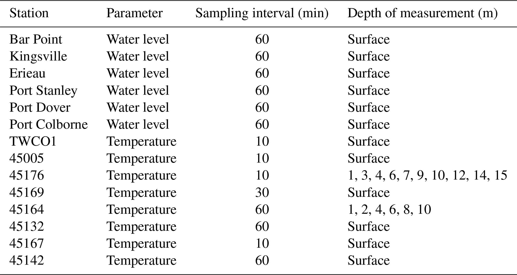
Eight in situ lake buoys, distributed over the nearshore areas of the three basins (Fig. 1; Table 1), provided near-real-time model validation data through the Great Lakes Observing System (GLOS: http://www.glos.us/, last access: January 2022) and National Data Buoy Center (NDBC: https://www.ndbc.noaa.gov/, last access: January 2022) portals. For each station, the text-based NDBC observations are parsed using the “BeautifulSoup” Python library, and the GLOS observations are retrieved using “webdriver” from the “selenium” Python library. All the lake buoy observations are saved as .csv files and read into MATLAB for post-processing. Attempts to retrieve missing variables would result in run-time errors.

The lake buoys are deployed from April or May to mid-October, spanning the spring/fall turnover and seasonal summer stratification periods. However, due to COVID-19-related delays in instrument deployments in 2020, only two buoys located offshore of Cleveland, near the water intake crib (station 45176 and station 45164), were equipped with thermistor chains to monitor temperature profiles. The other six buoys provide air and lake surface temperature as well as wind speed and direction observations for hydrodynamic and meteorological forecast validation. Satellite-based observations of lake surface temperature were obtained from the Great Lakes Surface Environmental Analysis (GLSEA2), which is derived from NOAA CoastWatch AVHRR (Advanced Very High-Resolution Radiometer) imagery and updated on NOAA GLERL website (https://coastwatch.glerl.noaa.gov/erddap/files/GLSEA_GCS/, last access: Deccember 2021). GLSEA2 produced daily observations, with 2.6 km resolution, from the cloud-free portions of the satellite images (Schwab et al., 1999). The NetCDF data are retrieved using the “BeautifulSoup” library and “webdriver” from “selenium”.

We quantified the temperature forecast capability using the statistical measures of RMSD (Eq. 1) and mean bias deviation (MBD):

$$\begin{array}{}\text{(3)}& \mathrm{MBD}=\mathrm{100}{\displaystyle \frac{\frac{\mathrm{1}}{N}{\sum }_{i=\mathrm{1}}^N(x_i-y_i)}{\frac{\mathrm{1}}{N}{\sum }_{i=\mathrm{1}}^N{y}_i}}.\end{array}$$

For the spatial MBD and RMSD (s-MBD and s-RMSD), x_i and y_i are the model and observed temperature in each grid, and N is the total number of grids. For time series MBD and RMSD (t-MBD and t-RMSD), x_i and y_i are the model and observed temperature at each sample time, and N is the total number of samples.

2.5 System operation

The COASTLINES operational forecast system is run on a local server supported by Queen's University ITS (Kingston, Canada). The COASTLINES workflow is presented in Fig. 2. The system consists of input data acquisition and preparation, 24 h hydrodynamic simulations, 240 h hydrodynamic simulations, validation against in situ observations, and uploading the model forecasts and validation to the web platform. Given that the standard deviations of meteorological forecast variables increase with forecast lead time (Buehner et al., 2015), we performed separate 24 and 240 h forecast simulations each day. The model advances every day according to the 24 h forecast simulation and terminates by generating “restart” files. These files are then used to hot start the 240 h forecast simulation and the 24 h simulations for the next day. The input files for the 240 h forecast simulations are iteratively replaced by the new 240 h meteorological forecast generated each day. The 24 and 240 h forecast model outputs are compared against observations to evaluate the forecast performance against forecast lead time.

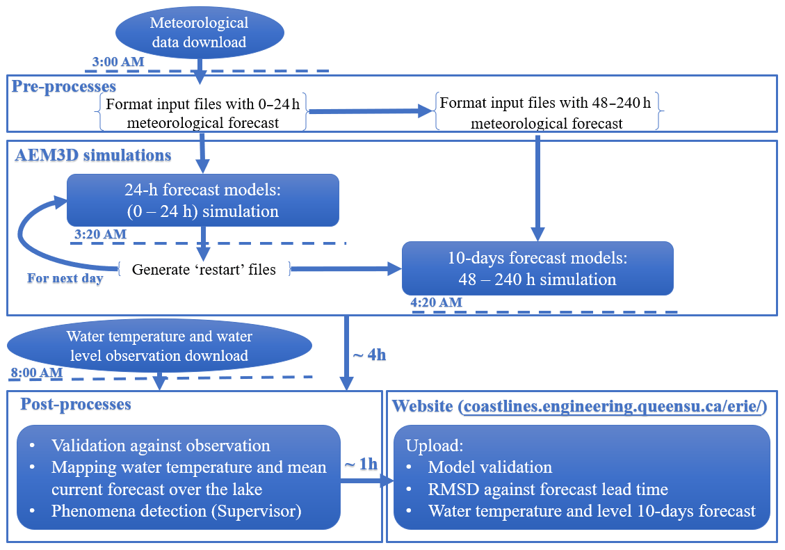
Figure 2 Daily workflow and automated processes in the COASTLINES operational system as performed on the local server.

The long-term stability of employing daily “hot” restarts can be seen in a comparison between simulated temperature profiles from a continuous run and that from stitching together the 24 h hot-start simulations (Appendix A; Fig. A1). At present, the initial water level cannot be modified using the AEM3D restart files. Therefore, to account for long-term drift in surface water level, we used real-time gauge observations as the datum point for water level forecasts (automatically performed by MATLAB in post-processing) and only consider errors resulting from simulation of storm surges and seiches, as opposed to those from seasonal changes in mean lake level. Automation of the processing tasks in the workflow is performed by Python scripts triggered by the Windows Task Scheduler every 24 h at midnight. The online meteorological forecast data are retrieved from GDPS once updated at 03:00 EST. Forcing variables are then formatted in MATLAB, called by the Python scripts once the meteorological forecast data have been retrieved. The AEM3D pre-compiled executable is then run as a black-box code, triggered by Python. The 24 and 240 h simulations take 0.5 and 4 h to complete, respectively. The observed data, including water levels from gauge stations, water temperatures from lake buoys, and satellite images, are scraped with Python at 08:00 EST, followed by post-processing in MATLAB to validate model output, calculate statistical metrics (RMSD, MBD), and generate figures. The results are exported to Google sheets and published to the COASTLINES website (e.g., Appendix B). The authors (supervisors of COASTLINES) and Queen's ITS monitor forecast results and maintain system operation.

Global coverage of the GDPS forecasts enables this operational system to be readily implemented at other sites where lake bathymetry, boundary flows, and in situ validation data are available. The workflow may be easily modified to include additional meteorological forecasts or other black-box hydrodynamic drivers (e.g., HRRR and Delft3D, respectively; Rey and Mulligan, 2021). This would require simple modification of the COASTLINES MATLAB-based write statements to meet the formatting requirements of a particular driver.

3 Results

The COASTLINES water level and temperature forecasts have been operational since April and July 2020, respectively. The 24 and 240 h forecast water levels from the 15 and 25 km resolution models were validated against real-time gauge station observations. The water level statistical metrics (RMSD and RE) were averaged over April to September 2020. The 24 and the 240 h forecast lake surface temperature and temperature profiles, from the models, were also validated against real-time lake buoy data and daily averaged satellite imagery. The time series and spatial MBD and RMSD (t-RMSD, t-MBD and s-RMSD, s-MBD) were averaged over July to September 2020.

3.1 Water level

The RE of the forecast water level increases with forecast time when averaged over April to September 2020; the 24 h forecast error being ∼ 40 % at all six gauge stations (Fig. 3a, c, e, g, i, k). Given the large water level fluctuation at Port Colborne (Fig. 3l), the 240 h forecast RE is highest at this station, exceeding 70 % (Fig. 3k). Of the six gauge stations reported in this study, those at the western (Bar Point and Kingsville) and eastern (Port Dover and Port Colborne) ends of Lake Erie longitudinal axis had the largest water level fluctuations, resulting from the predominant southwesterly winds generating strong wind setup and surface seiches (Fig. 3b, d, f, h, j, l). The lognormal means of the daily range in water level at the six gauge stations are 0.21 (Bar Point), 0.16 (Kingsville), 0.07 (Erieau), 0.10 (Port Stanley), 0.15 (Port Dover), and 0.17 cm (Port Colborne).

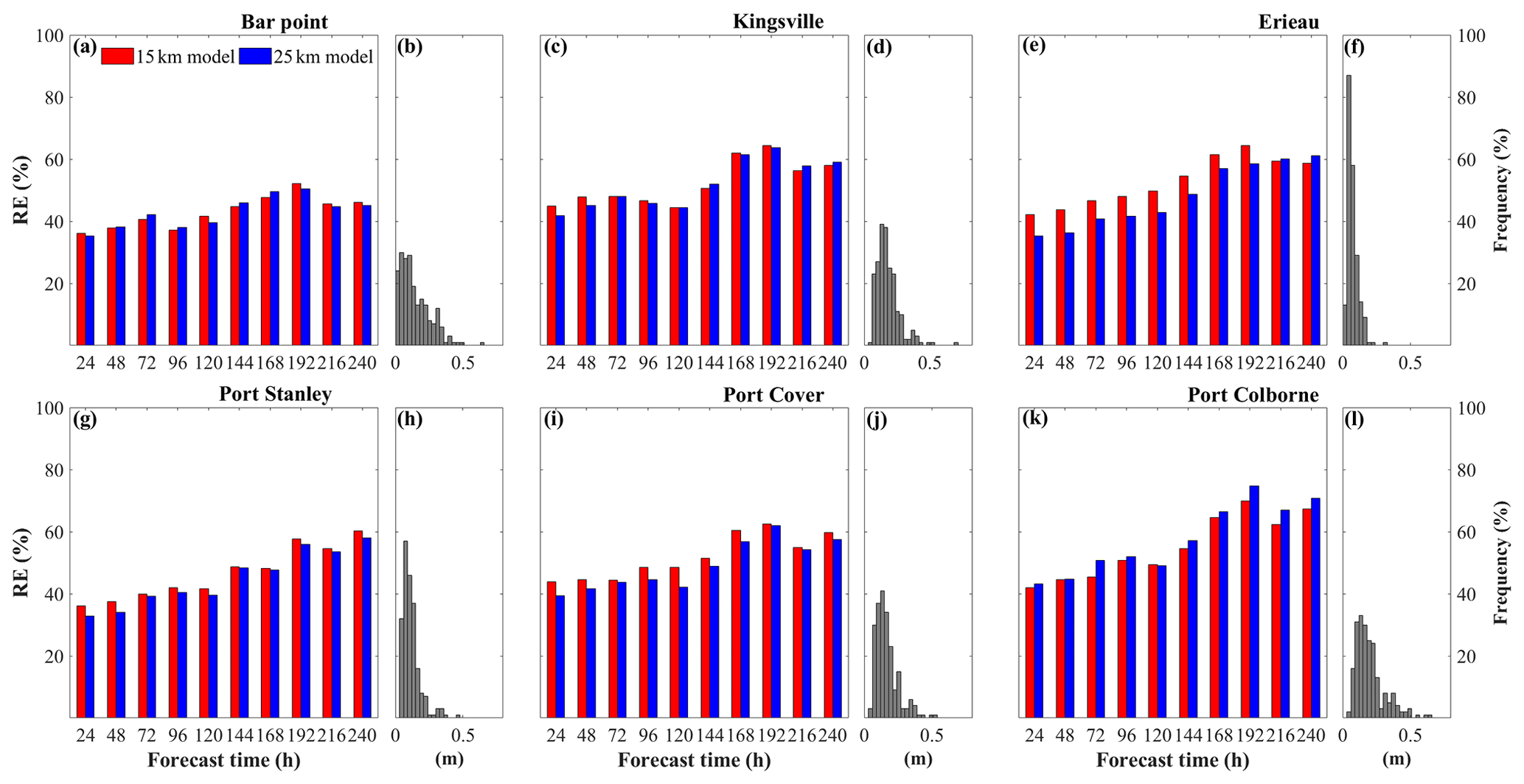
Figure 3 Relative error (RE) in water level predictions against forecast time at six stations (a, c, e, g, i, k). Panels (b), (d), (f), (h), (j), and (l) are the corresponding frequency distribution of lognormal means of the daily water level fluctuation range (x axes, unit: meters) at Bar Point, Kingsville, Erieau, Stanley, Port Dover, and Port Colborne, respectively.

The 24 h forecasts show qualitative agreement with observations in phase and magnitude (Fig. 4). The 24 h forecasts reproduce the dramatic surface seiches induced by westerly winds >15 m s⁻¹ (Fig. C2) on day 251 (RMSD <0.1 cm), especially the obvious water level fluctuations at stations in the western and eastern basins (Fig. 4a, b, e). However, the prediction of water level at Bar Point showed a large bias (Fig. 4f), with the model overestimating the water level fluctuation. The uncertainty in the model forecast, which increased with the range of the daily fluctuation, was captured by the 24 h forecast RE over April to September (the shaded areas in Fig. 4). Overall, the confidence interval of the 24 h forecast included most of the discrepancies between the observations and the model results.

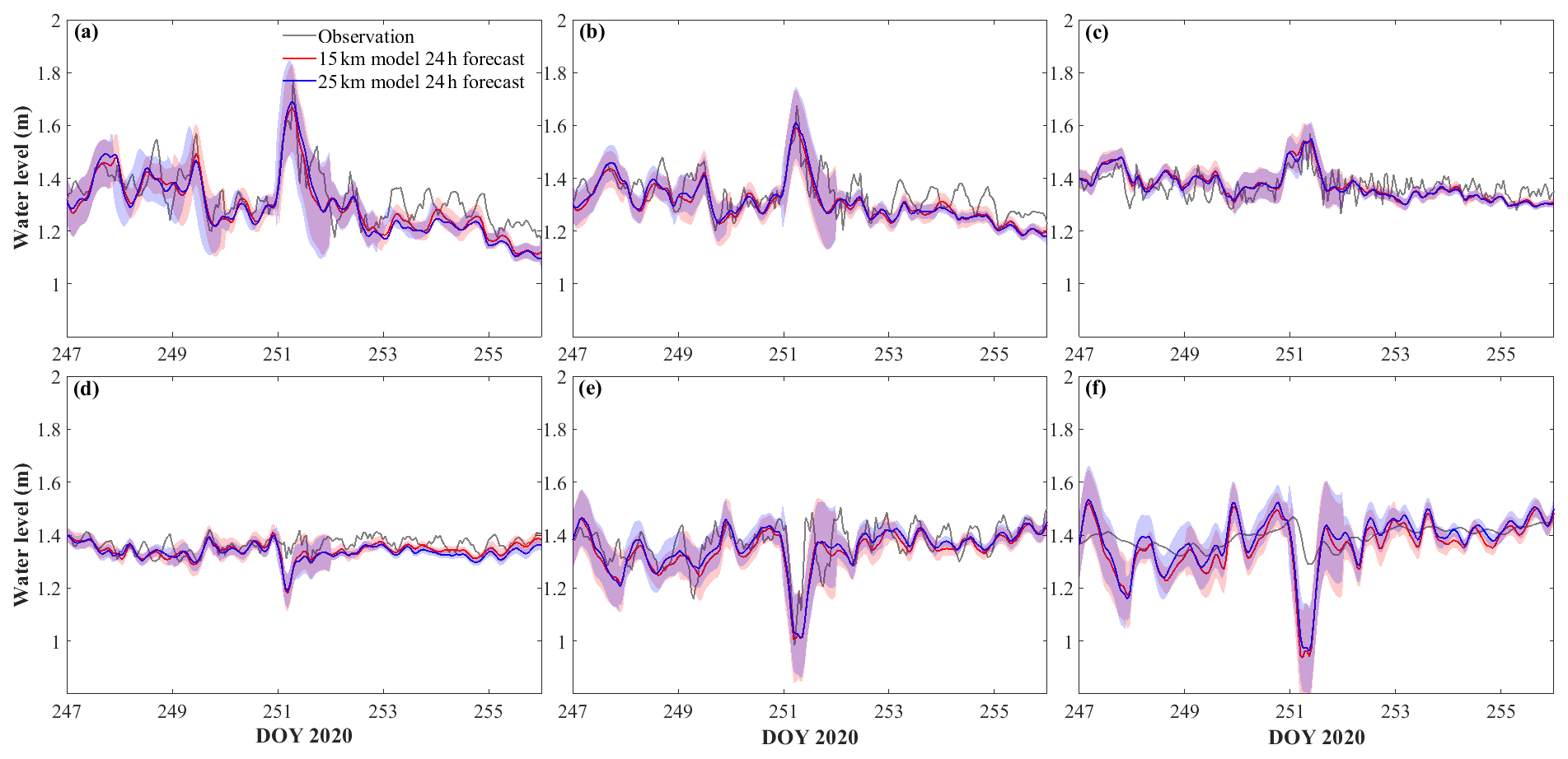
Figure 4 Comparison between observed and stitched 24 h forecast modeled water level at (a) Port Colborne, (b) Port Dover, (c) Port Stanley, (d) Erieau, (e) Kingsville, and (f) Bar Point. The shaded areas show the confidence interval of the 15 km model (red shading) and the 25 km model (blue shading), as given by the 24 h RE in Fig. 3.

Time series validations for the 240 h model forecast (Fig. 5) include confidence intervals from the RE (Fig. 3). As shown, the forecast began 6 d in advance of the large surface seiche event on day 251 and predicted the seiche to crest at Port Colborne 1–2 h ahead of the observations, and to trough at Kingsville 1–2 h behind the observations (Fig. 5a, c). Damping of the seiche oscillations (∼ 144 h in the future) was excessive, with the water levels being underestimated and the phase shifted by approximately 12 h (Fig. 5a, b). Despite the wide confidence intervals, due to the increasing RE with forecast time, large bias existed after the seiche event (forecast time >168 h). When the forecast was initiated close to the event (3 d before), the prediction of seiche phase was more accurate (Fig. 5d, e, f); however, the seiche decay still had a 12 h phase shift. The discrepancies in seiche amplitude (<0.1 m) were within the confidence intervals of the models.

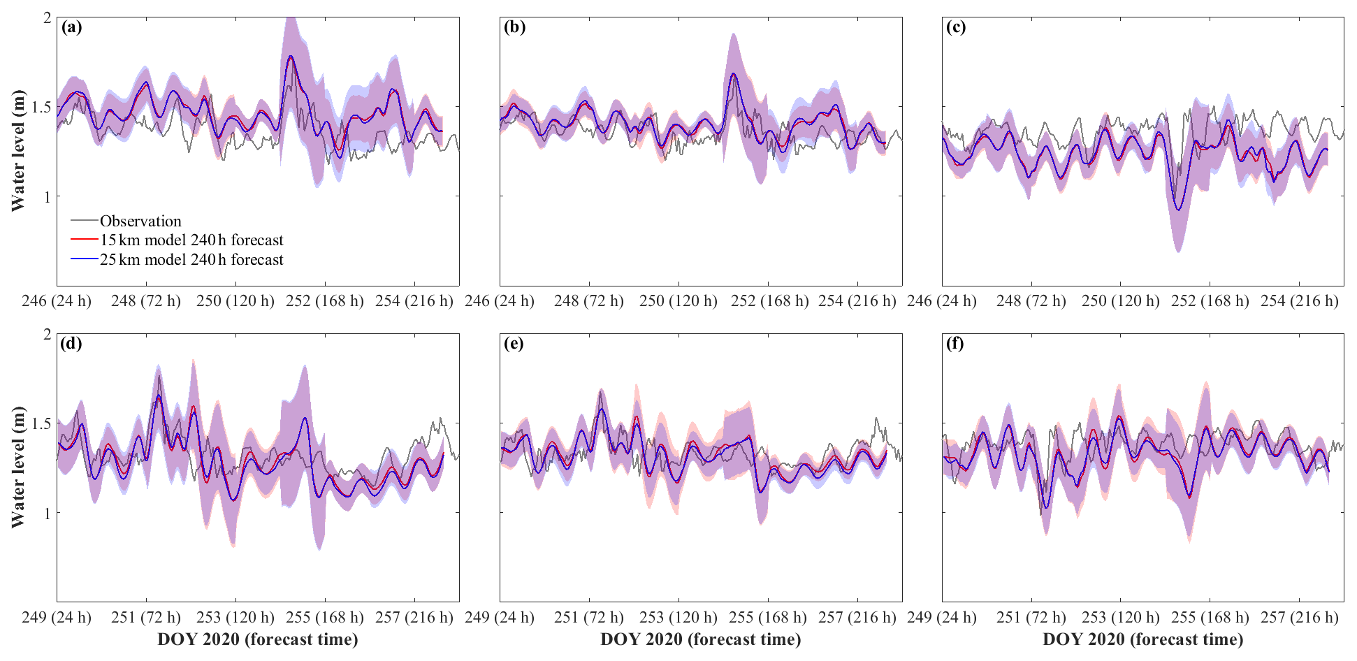
Figure 5 Comparison between the observed water level and 240 h forecast hot started on day 245 (a, b, c) and day 248 (d, e, f) at Port Colborne, Port Dover, and Kingsville, respectively. The shaded areas show the confidence interval of the 15 km model (red shading) and the 25 km model (blue shading), as given by the 240 h RE in Fig. 4.

3.2 Water temperature

3.2.1 Lake surface temperature

Using satellite-based and lake-buoy-based observations, we evaluated the lake surface temperature forecast (Fig. 6). The 24 h forecast captured the seasonal variation of lake surface temperature, particularly the rapid increase in temperature on days 180–190, and the gradual decrease in temperature after day 240, at all eight stations. However, the forecast overestimated the lake surface temperature in July by 3–5 ^∘C (days 180–210), particularly at stations (STNs) 45167 and 45142. Due to the 3 h output interval associated with the meteorological forecast data, the forecast model was insensitive to temperature fluctuations over shorter timescales, as recorded by the lake buoys, and it underestimated the sudden decrease in temperature near days 220 and 255 at STN 45005.

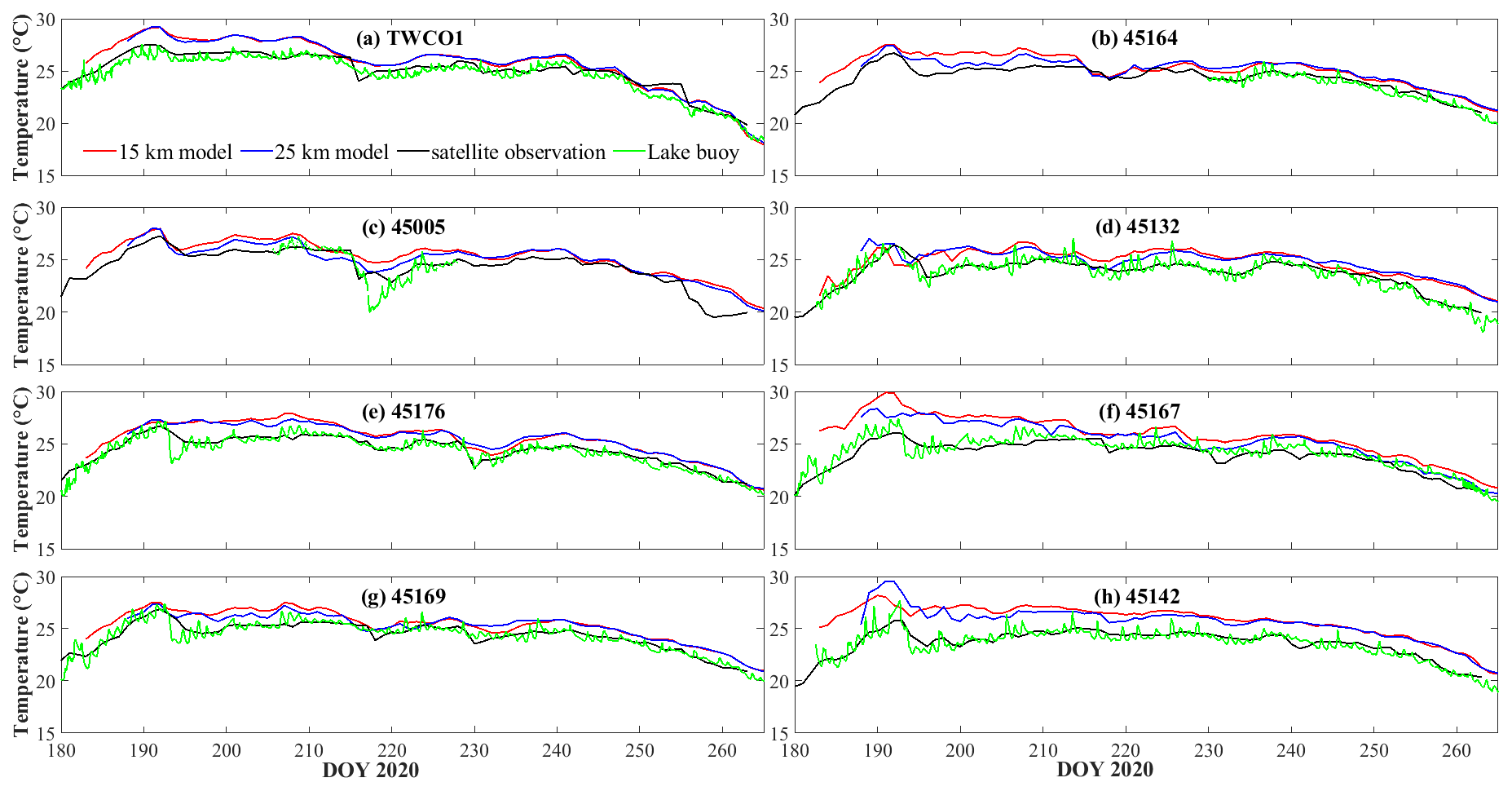
Figure 6 Comparison between the stitched 24 h forecast and observed lake surface temperature at eight stations (a) TWCO1, (b) 45164, (c) 45005, (d) 45132, (e) 45176, (f) 45167, (g) 45169, and (h) 45142. The green lines are time series observations from lake buoys; the black lines are daily observations derived from satellite imagery.

Overall, the t-MBD and t-RMSD, over these eight stations, were ∼ 6 % and 1.4 ^∘C (15 km model) and ∼ 5 % 1.3 ^∘C (25 km model) for the 24 h forecast, respectively (Table 2). The average s-MBD and s-RMSD over the 50 d from July–September were ∼ 4 % and 1.2 ^∘C, respectively, for both 15 and 25 km resolution models.

Table 2 Statistical measures of t-MBD (MBD) and t-RMSD (RMSD) between the 24 h forecast model and observations of water temperature.

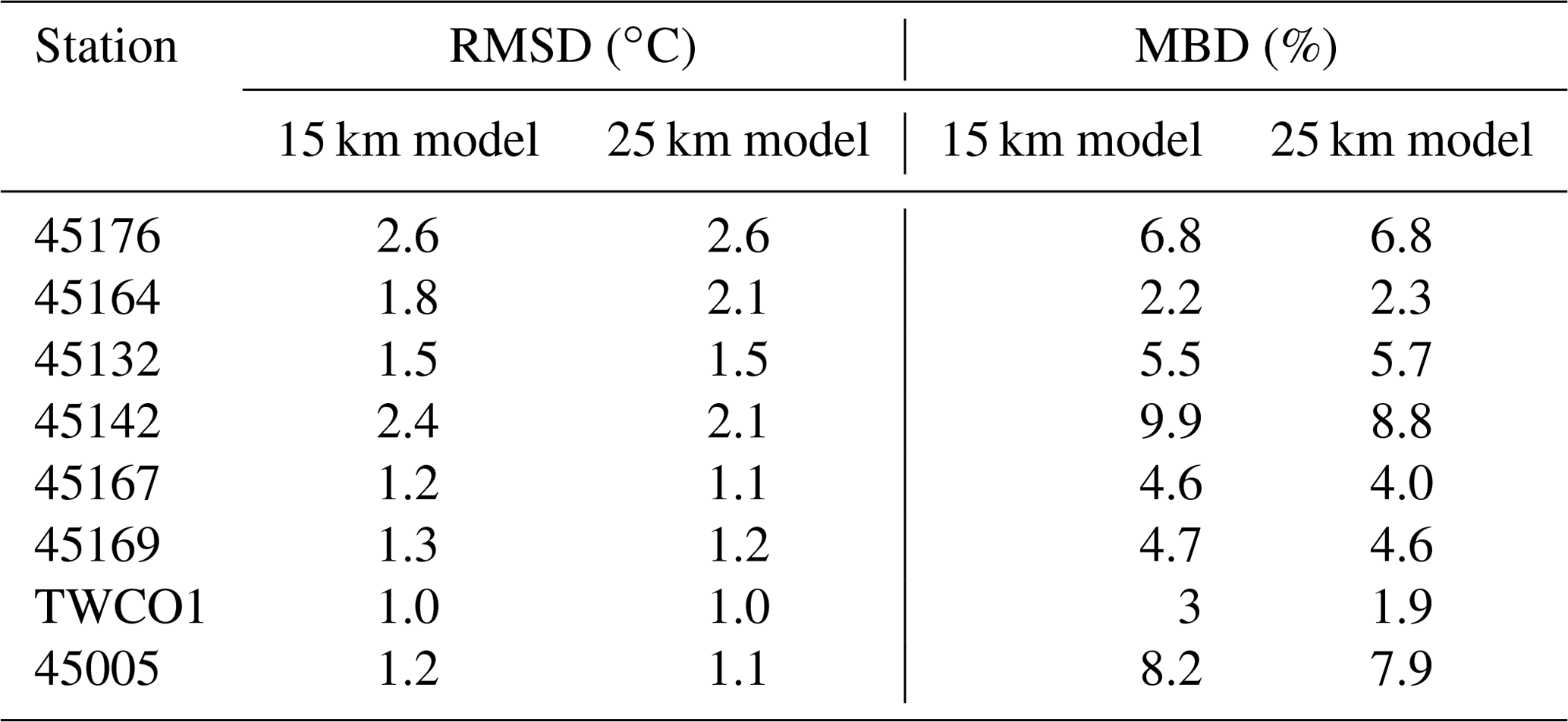
The 240 h forecast MBD and RMSD, surprisingly, do not show an increase in error with forecast time (Fig. 7a, b). Both t-MBD and s-MBD, over the 240 h forecast, are ∼ 4 %–5 %, with s-MBD 0.5 %–1 % higher than t-MBD. Although both 240 h s- and t-RMSD are under 2 ^∘C, the t-RMSD show the error with forecast time to be higher than s-RMSD. Both time series observations from lake buoys and daily averaged observations from satellite imagery fall into the forecast confidence interval based on the 240 h t-RMSD (Fig. 7c–f).

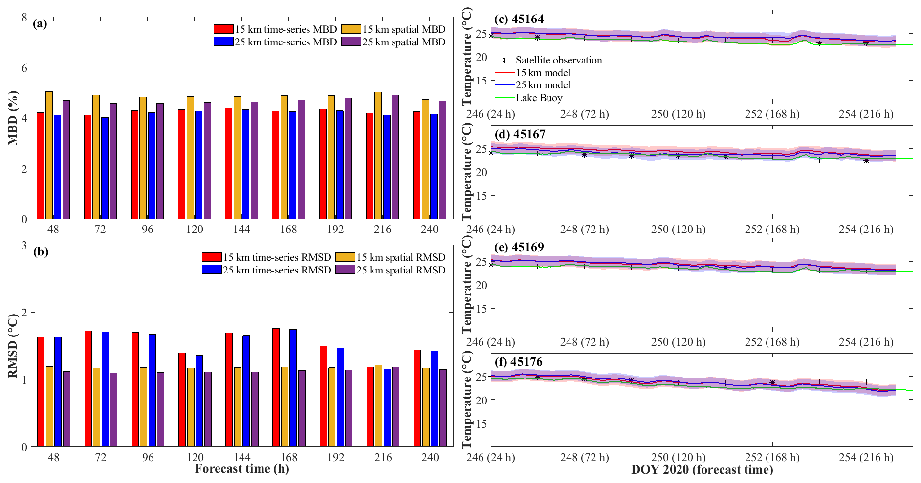
Figure 7 (a) MBD against forecast time; (b) RMSD against forecast time. (c–f) Time series of 240 h forecast and observed lake surface temperature at stations 45164, 45167, 45169, and 45176, respectively, and daily averaged satellite lake surface temperature (black asterisks). The confidence interval (shaded areas) in panels (c)–(f) represents the uncertainty of the 240 h forecast model through the time series RMSD with the forecast time (panel b).

Spatial comparisons of satellite-based observations to the 24, 48, 120, and 168 h surface temperature forecasts illustrate that the forecast system (with 15 km meteorological data) predicted the cooler water mass along the northwest shoreline of the central basin with a cold bias ∼ 2 ^∘C (Fig. 8); this may be upwelling hypolimnetic water (see following Sect. 4.2). The model also predicted lower surface temperatures in coastal regions of the western basin with a cold bias ∼ 2 ^∘C (Fig. 8m–t); the bias presumably was induced by neglecting riverine inflows (e.g., Detroit River and Maumee River; see also Sect. 4.3), which are typically near the air temperature and several degrees warmer than the lake surface (Wang and Boegman, 2021). Further comparisons between model predictions and satellite-based observations of lake surface temperature can be found in Appendix D (Figs. D1–D2).

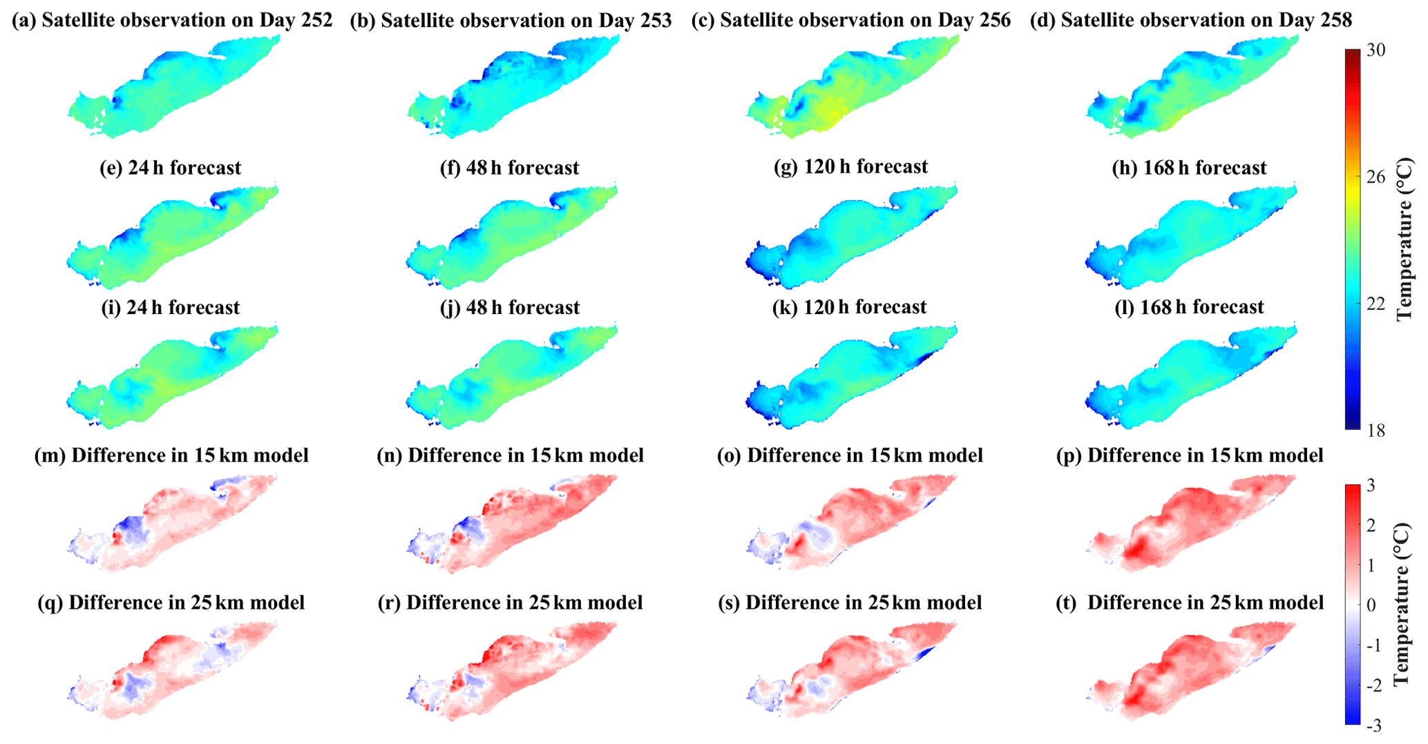
Figure 8 Comparison of lake surface temperature from (a–d) satellite observations, (e–h) 15 km model forecast, and (i–l) 25 km model forecast during late summer. The models were hot started on day 251. The differences between observations and models are shown in panels (m)–(t).

3.2.2 Thermal structure

The 3-D AEM3D model structure applied in COASTLINES enables the prediction of the thermal profiles in the lake. On 15 June 2020 (day 168), a rapid drop (∼ 6 ^∘C) in surface temperature was recorded by the thermistor at STN 45176 and predicted by the stitched 24 h COASTLINES model (15 km meteorological input) (Fig. 9a, b). The timing and intensity of this upwelling event were accurately forecast, but before and after the upwelling event, the mixed layer depth was modeled to be deeper than observed, which is perhaps a result of spurious numerical diffusion resulting from the thermocline swashing along the stair-step z-level grid at the lake perimeter. The 240 h forecast model was not yet operational at this time.

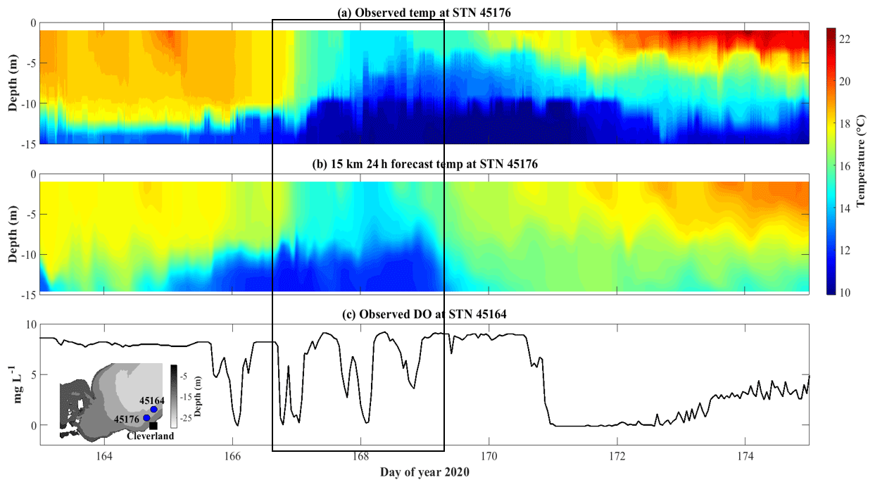
Figure 9 Temperature profile comparisons between (a) observations and (b) stitched daily 24 h forecasts from the 15 km resolution model at station 45176. (c) Observed dissolved oxygen concentration at station 45164 from lake buoy (http://www.glos.us/, last access: December 2021). The inset image shows the bathymetry and locations of lake buoys. The black square indicates the timing of the upwelling event.

Both the 240 h 15 and 25 km resolution forecasts predicted the downwelling event on 11 July 2020 (day 193) at STN 45176 (Fig. 10). The forecasts were hot started 7 d before the event (day 187), successfully predicting when warm surface water downwelled toward the bed displacing the thermocline (Fig. 10b, c), but the 15 km resolution underestimated the intensity of downwelling, predicting thermocline recovery on day 193. The forecast hot started 5 d before the event (day 189) gave a more accurate prediction with the downwelling persisting over 2 d (Fig. 10d, e) – as observed (Fig. 10a).

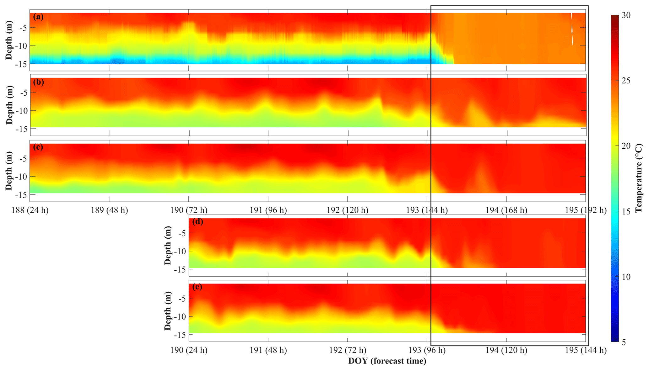
Figure 10 Comparisons of (a) observed temperature profile, (b, d) 240 h 15 km resolution modeled, and (c, e) 240 h 25 km resolution modeled temperature profiles at STN 45176. The forecast models were hot started on day 187 (b, c) and day 189 (d, e). The black square indicates the downwelling event.

4 Discussion

4.1 Prediction of coastal upwelling for fishery and drinking water management

The central basin of Lake Erie is vulnerable to hypoxia in summer from near-bed thermal stratification and the relatively large ratio of sediment area to hypolimnetic volume (Bouffard et al., 2013; Nakhaei et al., 2021). Associated fish-kill events (tens of thousands) are regularly reported, including an event on north shore of the central basin in the late summer of 2012, which was presumably was caused by upwelling of cold anoxic water from the hypolimnion (MOE, 2014; Rao et al., 2014). Similarly, thousands of freshwater drum were killed in a rapid warming event (∼ 5 ^∘C per week) in the western basin in 2020 (https://www.13abc.com/content/news/Hundreds-of-dead-fish-wash-up-in-Sandusky-Bay-571025541.html, last access: June 2020). Similarly, shoreward advection of hypoxic water, from upwelling or internal waves, also adversely affects source water quality at drinking water intakes (https://epa.ohio.gov, last access: August 2020), whereby high Fe and Mn or low pH, associated with hypoxic water, requires adjustment of treatment processes. This is a particular issue along the Ohio coast of the central basin (Ruberg et al., 2008; Rowe et al., 2019).

The ability to predict these movements of hypolimnion water would aid management of both Lake Erie fisheries and drinking water treatment. Here, we test the ability of the model to predict upwelling of cold bottom water in the region where the fish kill was observed in 2012. On days 249–253 in 2020 (Fig. 8), strong southwesterly winds (∼ 12 m s⁻¹; Fig. C2) were modeled and observed to create upwelling along the north shore, as expected from Ekman drift of the surface layer (Jabbari et al., 2019). The upwelled cold hypolimnetic water is shown near the coast of Erieau in the satellite observations and the 15 km resolution model (Fig. 8a, b, e, f). The depth-averaged water temperature and current circulation in the forecast show upwelling to persist for several days (Fig. 11), with cold hypolimnetic water accumulating along the north shore and strong eastward currents along the northern shoreline of the east-central basin. The upwelling region matched that shown in a 2013 hindcast simulation (Valipour et al., 2019), revealing the hotspots of vertical transport of nutrients and anoxic hypolimnetic water.

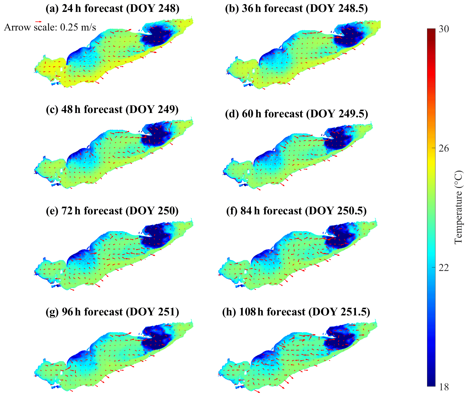
Figure 11 Color maps showing the forecast depth-averaged temperature throughout the lake. The red arrows represent forecast depth-averaged currents. The model results are from the 240 h forecast model hot started on day 247.

Another upwelling event occurred near the Cleveland drinking water intake crib on days 167–170 (Fig. 9). This event was accompanied by simultaneous ∼ 8 mg L⁻¹ oscillations in the observed dissolved oxygen concentration (Fig. 9c) at STN 45164 (∼ 20 km away from STN 45176), followed by the dissolved oxygen concentration becoming locally hypoxic (<2 mg L⁻¹) for ∼ 2 d. The COASTLINES model predicted this event (Sect. 3.2.2), which would have provided sufficient notice for drinking water plane operators to implement the additional treatment required for hypoxic water (Rowe et al., 2019). Future work, using the coupled iWaterQuality biogeochemical module (formerly CAEDYM) could extend COASTLINES to forecast water quality in Lake Erie (León et al., 2011), including dissolved oxygen concentrations and formation of algae blooms (Bocaniov et al., 2020).

4.2 Prediction of storm-surge events for public safety

Due to its shallowness and long fetch aligned with the predominant southwest winds (Hamblin, 1979), Lake Erie has the largest daily range of water level amongst the Great Lakes (Trebitz, 2006); these water level fluctuations are mainly due to storm surges and surface seiches (Mortimer, 1987). In every month of 2020, Lake Erie set new mean water level records (https://www.tides.gc.ca/C&A/bulletin-eng.html, last access: December 2020), causing the shoreline to be exposed to high risk from erosion and flooding and making the shoreline communities susceptible to costly damage and economic loss (e.g., https://www.lowerthames-conservation.on.ca/flood-forecasting/flood-notices/, last access: December 2020). Given the ability of COASTLINES to predict water level fluctuations induced by storm surges and seiches (Figs. 3, 5), we tested the ability of the model to act as a coastal flooding warning system. Due to the unpredictability and severity of water level fluctuations in Lake Erie, there is currently a need to improve short-term water level forecasts and water level warning systems (Gronewold and Rood, 2019). This would assist early decision-making during natural hazards (Gronewold and Rood, 2019).

We forecast the storm event on 15 November 2020, which generated a wind-induced storm surge (∼ 1–1.5 m) in the eastern basin with associated strong surface currents (Fig. 12). The inset image, taken during the event, shows the coastal flooding from this event. COASTLINES successfully predicted the high-water-level phase at Port Dover 72 h in advance but underestimated the water level increase by 0.5 m. The hot-start forecast 24 h in advance was more accurate in predicting the water level prediction, with a difference <0.5 m from the observations (Fig. 12d). Note that both forecasts missed the small (∼ 0.5 m) seiche before the significant increase at the end of day 320, presumably due to the low temporal resolution of the meteorological forecast input or local topography near the gauge. The overall wind-induced tilt of the free surface was lower from the 72 h hot start relative to the 24 h hot start (Fig. E1), which predicted a larger local storm surge (Fig. 12d).

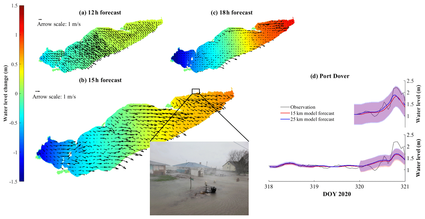
Figure 12 Color maps showing the water level change compared to 15 November at 00:00 EST from (a) 12 h, (b) 15 h, and (c) 18 h forecasts from the 15 km resolution model. The black arrows are depth-averaged mean current fields. Panel (d) shows a comparison between forecast and observed water level at Port Dover. The upper panel shows the forecast hot started on 15 November 2020 (day 320), and the lower panel shows the forecast hot started on 12 November 2020 (day 317). The shaded region indicates the confidence interval. The inset image (extracted from a footage by Jason Homewood​​​​​​​ from Lower Thames Valley Conservation Authority) shows the flooding induced by the dramatic water level increase during this event. The two cottages shown in the images were destroyed later in the afternoon.

The impacts of coastal flooding could be improved by including simulation of wind waves through enabling the coupled surface wave model SWAN (Booij et al., 1999) in AEM3D. Similarly coupled Delft3D-SWAN models have recently been applied in the development of a real-time predictive system for the coastal ocean and large estuaries (Rey and Mulligan, 2021).

4.3 Bias and uncertainty

The AEM3D model (formerly ELCOM) employed in COASTLINES has shown skill in temperature hindcasts in the Great Lakes with RMSD ∼ 0.9–3 ^∘C in Lake Erie (Liu et al., 2014; Oveisy et al., 2012) and 1.5–1.9 ^∘C in Lake Ontario (Paturi et al., 2012). Similarly, the 24 h COASTLINES forecast predicted water temperatures with an average s-RMSD and t-RMSD <2 ^∘C at the surface (Table 2). Therefore, the forecasts are within ∼ 1 ^∘C RMSD in comparison to hindcasts, showing sufficient model skill for predictive simulations to aid lake management (movements of hypoxic water, fish thermal habitat, etc.). The accuracy of the COASTLINES forecasts may result from the high spatial resolution and coverage of meteorological forecast compensating for the inherent inaccuracies in the weather forecast data. Errors in forcing data may be compensated for using data assimilation (Baracchini et al., 2020b). In the hindcast models, Liu et al. (2014) applied uniform Lake Erie meteorological forcing over four zones and Valipour et al. (2019) utilized six zones, each spanning ∼ 100 km. These included land-based observations, when there was no available lake buoy data, which induce error, especially in large shallow lakes (Hamblin, 1987). The comparatively high-resolution GDPS meteorological forecast was 4–5 times higher in horizontal resolution than used in the hindcast simulations, improving the representation of regional meteorological and climatological conditions.

Compared to other operational lake forecast systems, the 240 h COASTLINES forecast is longer (e.g., GLCFS forecasts 120 h and meteolakes.ch forecasts 108 h) and is the only one forced with open-access meteorological data that have global coverage. The GLCFS provided 48 h water level forecasts with RMSD ∼ 0.12 m at the Buffalo gauge and ∼ 0.14 m at the Toledo gauge, corresponding to RE ∼ 60 % and 51 %, respectively (O'Connor et al., 1999; Trebitz, 2006), using the older 4 km grid Princeton Ocean Model implementation, as opposed to the newer unstructured grid FVCOM GLCFS. COASTLINES gives better 48 h water level forecast performance (RE ∼ 40 %) at six gauge stations. For temperature, benefitting from a smaller domain, finer-resolution meteorological input (∼ 2.2 km), and data assimilation, the 4.5 d lake surface temperature predicted by meteolakes.ch has a RMSD = 0.8 ^∘C (Baracchini et al., 2020b), whereas COASTLINES predicted the 120 h (5 d) lake surface temperature with RMSD ∼ 1.7 ^∘C. COASTLINES also outperforms 1-D climatological hindcasts (e.g., Freshwater Lake; FLake), with 2–4 ^∘C RMSD over a 120 h lake surface temperature forecast (Lv et al., 2019; Gu et al., 2015) and has similar error to the 3-D Princeton Ocean Model (Kelley et al., 1998), with 0.6–0.9 ^∘C mean absolute error in the 36 h lake surface temperature forecast at station 45005.

The uncertainty and bias in the COASTLINES forecast result from error induced by the initial conditions at each hot start, error in the meteorological forecasts, and error in the numerical methods. These errors could be reduced by improving model calibration through data assimilation. For example, Baracchini et al. (2020b) reduced the RMSE temperature simulation of Lake Geneva from ∼ 2 to ∼ 1 ^∘C by employing a sequential data assimilation routine; this would correspond to a <5 % improvement in simulation of Lake Erie summer surface temperature. In AEM3D, sequential data assimilation could be implemented through modification of the restart files (aem3d_restart_v3_type.f90); however, this is beyond the scope of the present study. Future work will focus on adding real-time model calibration (e.g., Gaudard et al., 2019), which is not presently included in the COASTLINES forecast workflow. For example, Baracchini et al. (2020a) employed OpenDA as a black-box wrapper to calibrate Delft3D for Lake Geneva.

The errors induced by hot starting were shown to be negligible (Figs. 4, 6, 7a, b, A1). However, uncertainty from boundary conditions, especially the meteorological forcing, may introduce error. The 23 to 31 meteorological zones from the forecast wind field provides spatial variability required to simulate the mean surface circulation (Laval et al., 2003), water level (Trebitz, 2006), and thermocline motions (Valipour et al., 2015, 2019). However, the 3 h time interval between GDPS forecast dataset updates is much less than the 10 min interval associated with meteorological data observed at lake buoys (typically one to six) used to drive hindcasts (e.g., León et al., 2005) and so the coarse temporal resolution in the GDPS forecast may alias temporal events, such as wind gusts (Fig. C1). This is of particular concern in large shallow lakes, such as Lake Erie, where winds play the dominant role in driving hydrodynamics. The rapid response of the water level to windstorms (Hamblin, 1987) could result in the effects of aliasing and forecast error being passed to the water level, leading to the growth of RE against forecast time (Fig. 3). The meteorological forecast from the 15 and 25 km GDPS models did not show discrepancies (Figs. C2–C5) and the evaluation metrics indicate that forecast results were largely insensitive to the meteorological inputs in Lake Erie (Figs. 3, 7). However, the 15 km model better predicted the mesoscale upwelling event (Figs. 8, 9, D2). The 24 h air temperature and wind speed forecasts had ∼ 1.5 ^∘C and ∼ 2 m s⁻¹ RMSDs, respectively. However, bias in the 240 h forecast increases with forecast time (Buehner et al., 2015). The 168 h forecast meteorological data overestimated wind speeds by up to 10 m s⁻¹ (Fig. C4), and bias in the air temperature forecast (Fig. C5) may cause the consistent warm bias (up to 3 ^∘C) in forecast lake surface temperature (Fig. 8). These errors may be corrected through real-time calibration using data assimilation (Baracchini et al., 2020a, b). The growing bias in air temperature, with forecast time, does not affect the lake surface temperature (Fig. 7), presumably due to the buffer effect of surface mixing layer (Schertzer et al., 1987).

Neglecting the inflows and outflows in the predictive simulation could induce bias in the forecast. The overestimation of water level fluctuation range near Bar Point (Fig. 4f) may result from neglecting the large Detroit River inflow, which regulates the seiche magnitude. The inflows also adjust more rapidly to air temperatures compared to deep lake waters. Thus, the up-to-2 ^∘C cold bias in coastal regions of the western basin (Figs. 8m–t, D2) could be induced by neglecting the heated flux from two major inflows (i.e., Detroit River and Maumee River) of Lake Erie.

In addition to inaccuracy in initial and boundary conditions, the discrepancies in simulating temperature profiles forecast may result from numerical diffusion arising due to the discrete nature of the vertical and horizontal grids. The simulated thermocline depth is overestimated (Figs. 9, 10), as in applications of ELCOM with both higher (Nakhaei et al., 2019) and lower resolution (Paturi et al., 2012). COASTLINES has the potential to predictively simulate mesoscale physical processes, such as Kelvin waves (Bouffard and Lemmin, 2013) and nearshore–offshore exchange (Valipour et al., 2019); however, model performance is poor in nearshore areas, where topographic features remain poorly resolved.

5 Conclusions

We developed an operational forecast system, COASTLINES, using the Windows Task Scheduler, Python-based data scrapping/formatting, and MATLAB data processing scripts, to automate application of a black-box hydrodynamic driver (AEM3D) to Lake Erie as an operational forecast tool. The resulting real-time and predictive lake modeling system used meteorological forecasts to generate 240 h forecasts of the lake surface level and 3-D temperature and current fields on a 500 m × 500 m (horizontal) × ∼ 1 m (vertical) grid, compares model output with near-real-time observations, and publishes the model output on a web-based platform.

The favorable agreement between forecast model results and observed physical variables (e.g., water level RE ∼ 40 % and temperature t-RMSD and s-RMSD <2 ^∘C) in Lake Erie demonstrates the ability of the forecast system to make predictions of hydrodynamic processes on time horizons up to 240 h that are as accurate as traditional hindcast simulations using directly observed meteorological forcing. This enables the near-real-time updates to the web platform to be used as a communication tool that rapidly disseminate forecast results to managers and stakeholders. Examples include >24 h prediction of (i) up- and downwelling events leading to fish kills; (ii) upwelling events transporting hypoxic water to a drinking water intake; and (iii) coastal flooding events from storm surges.

This operational system shows the feasibility of applying freely available meteorological forecasts (e.g., GDPS, HRRR), in situ buoy data, and satellite images to drive and validate any computational lake model (e.g., AEM3D, Delft3D, GLM), without modifying the source code. The global coverage of the weather model allows generalization of model application to lake or coastal domain. To facilitate further development of open-access predictive modeling systems, agencies are encouraged to share model validation observations, in real time, through organizations such as GLEON (https://gleon.org/, last access: December 2021) and GLOS (http://www.glos.us, last access: December 2021). This will enable extension of COASTLINES to include prediction of the physical–biogeochemical variables that drive sediment transport, hypoxia, and harmful algal blooms.

Appendix A: Comparison of 24 h model run with restart files and model run with continuous files

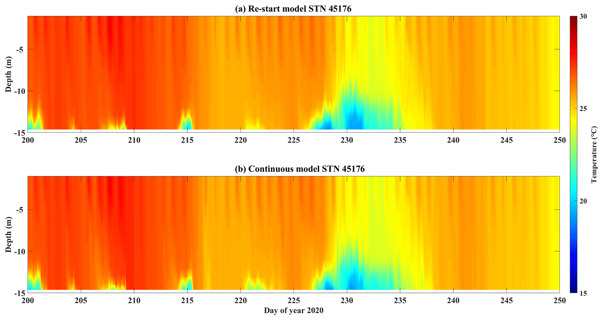
Figure A1 Temperature profile comparison between (a) stitched 24 h model run with restart files and (b) the model run with continuous input files.

Appendix B: COASTLINES website snapshot

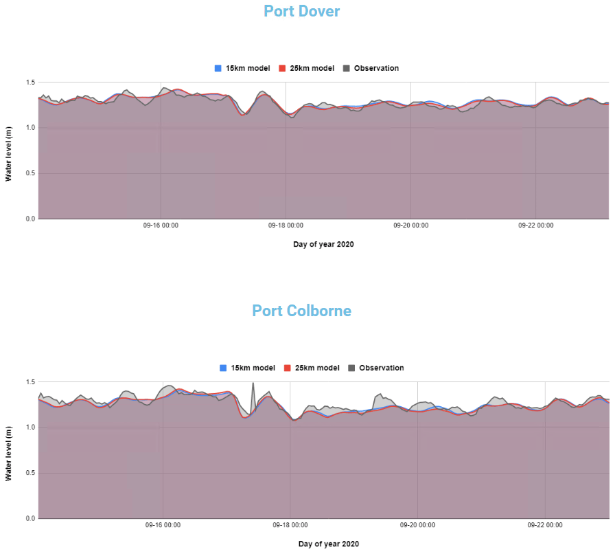
Figure B1 Snapshot of water level forecast validation web page displayed on the COASTLINES online platform: https://coastlines.engineering.queensu.ca/erie/water-level-forecast (last access: December 2021​​​​​​​) (status on 23 September 2020).

Appendix C: Validation of meteorological input variables

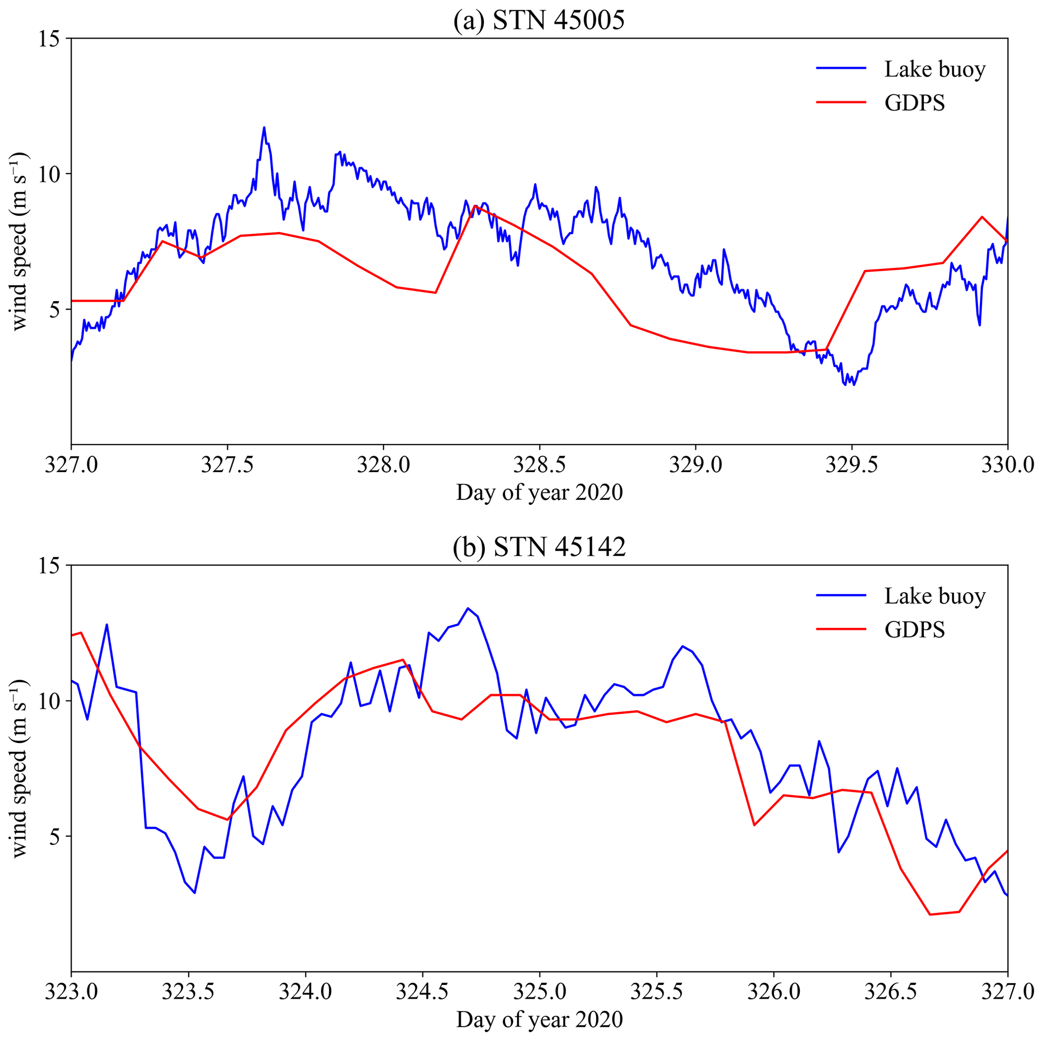
Figure C1 Comparisons of stitched GDPS wind forecast with 3 h delivery interval and lake-buoy-measured wind speed at (a) station 45005 (10 min sampling interval) and (b) station 45142 (1 h sampling interval). The wind gusts on day 327 at station 45005 and day 324 at station 45142 were missed by the wind forecast.

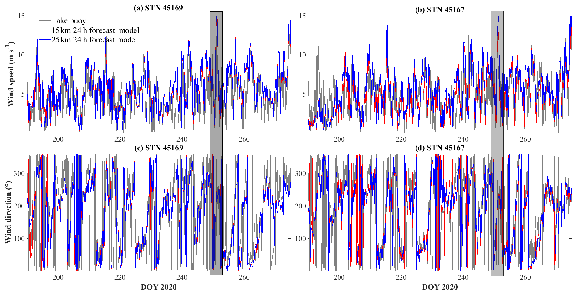
Figure C2 Comparisons of 24 h meteorological forecast and lake buoy observations of wind speed (a, b) and wind direction (c, d). The gray rectangle indicates the storm that led to upwelling along northern shoreline on days 248–253.

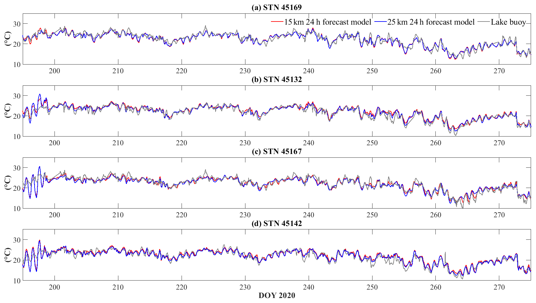
Figure C3 Comparisons of 24 h air temperature forecast and lake buoy observations of air temperature.

Figure C4 Comparisons of 240 h meteorological forecast and lake buoy observations of wind speed (a, b) and wind direction (c, d).

Figure C5 Comparisons of 240 h air temperature forecast and lake buoy observations.

Appendix D: Temperature validation against satellite observations

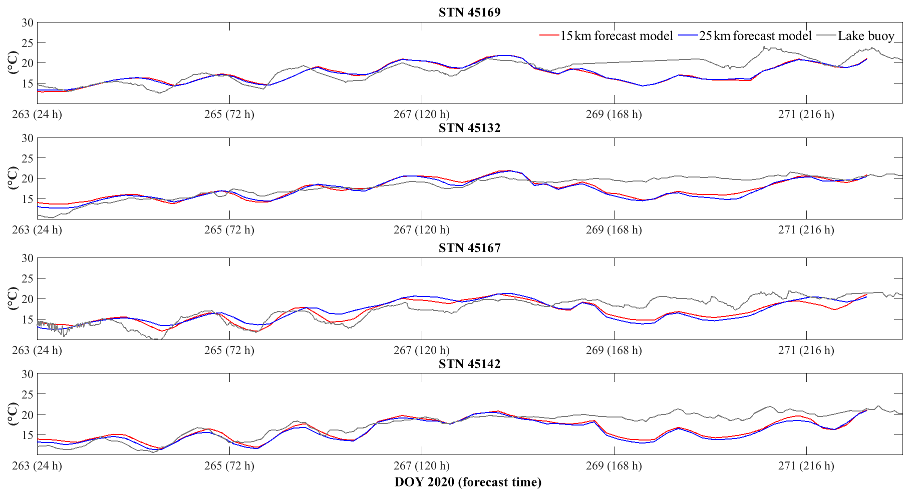
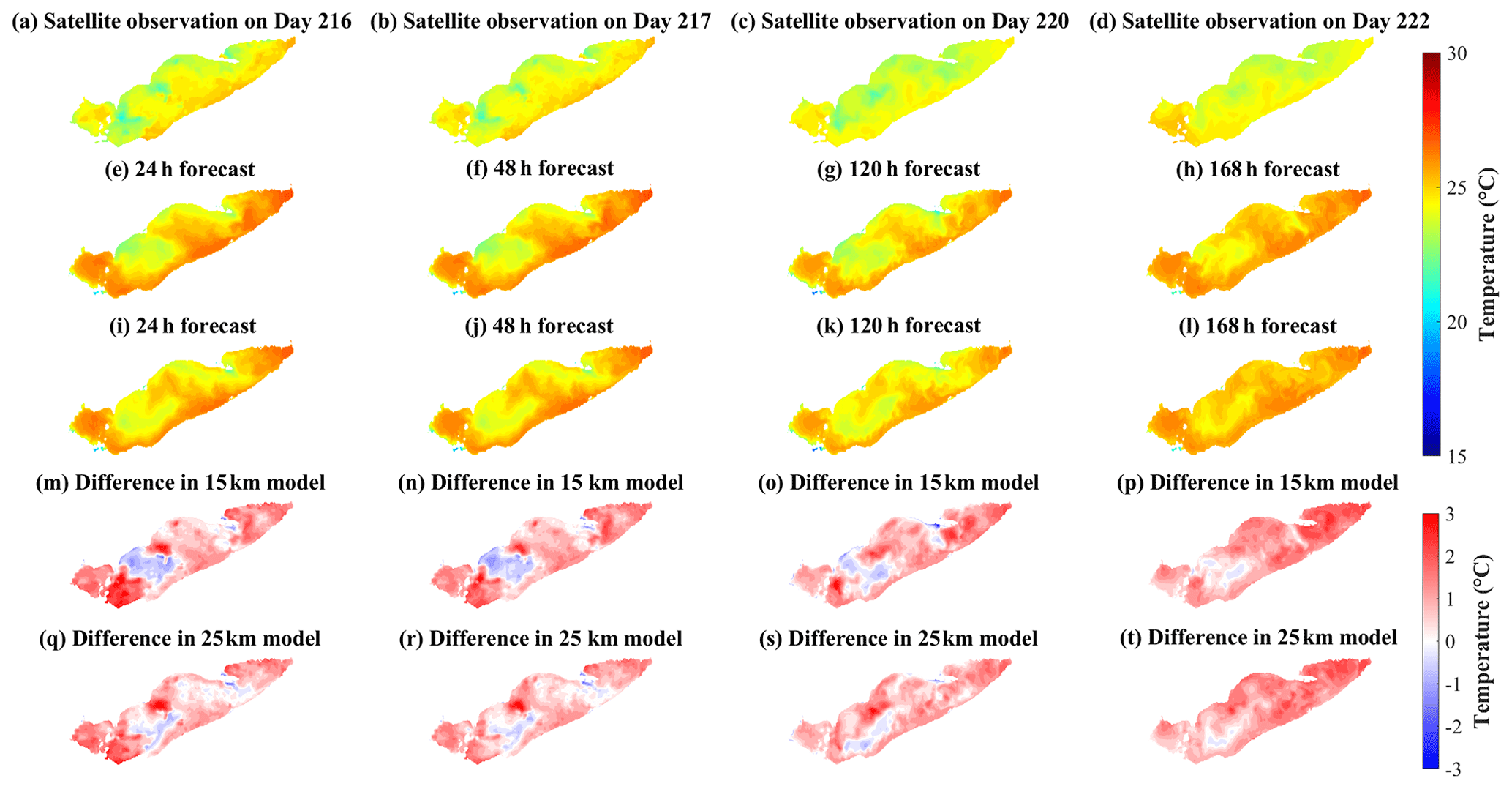
Figure D1 Comparisons of (a–d) satellite observations, (e–h) 15 km model 240 h forecast, and (i–l) 25 km model 240 h forecast during summer. The models were hot started on day 215. The differences between observations and models are shown in panels (m)–(t).

Figure D2 Comparisons of (a–d) satellite observations, (e–h) 15 km model 240 h forecast, and (i–l) 25 km model 240 h forecast during late summer. The models were hot started on day 244. The differences between observations and models are shown in panels (m)–(t).

Appendix E: Water level change during the windstorm on 15 November 2020

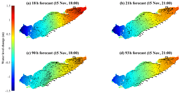
Figure E1 Spatial distribution of water level change from forecasts hot started on 15 November (a, b) and 12 November (c, d). The water level on 15 November at 00:00 EST is the reference level. The black arrows are depth-averaged mean current fields. The black squares in the upper right corners of each map indicate the location of Port Dover (Fig. 12d).