the Creative Commons Attribution 4.0 License.
the Creative Commons Attribution 4.0 License.
 | 01 Dec 2021
Recalculation of error growth models' parameters for the ECMWF forecast system
Aleš Raidl
Jiří Mikšovský
This article provides a new estimate of error growth models' parameters approximating predictability curves and their differentials, calculated from data of the ECMWF forecast system over the 1986 to 2011 period. Estimates of the largest Lyapunov exponent are also provided, along with model error and the limit value of the predictability curve. The proposed correction is based on the ability of the Lorenz (2005) system to simulate the predictability curve of the ECMWF forecasting system and on comparing the parameters estimated for both these systems, as well as on comparison with the largest Lyapunov exponent (λ=0.35 d−1) and limit value of the predictability curve (E∞=8.2) of the Lorenz system. Parameters are calculated from the quadratic model with and without model error, as well as by the logarithmic, general, and hyperbolic tangent models. The average value of the largest Lyapunov exponent is estimated to be in the < 0.32; 0.41 > d−1 range for the ECMWF forecasting system; limit values of the predictability curves are estimated with lower theoretically derived values, and a new approach for the calculation of model error based on comparison of models is presented.
- Article
(4497 KB) - Full-text XML
- BibTeX
- EndNote


Forecast errors in numerical weather prediction systems grow in time because of the inaccuracy of the initial state (initial error), chaotic nature of the system itself, and the model imperfections (model error). The growth of forecast error in weather prediction is exponential on average. As an error becomes larger, its growth slows down and then stops, with the magnitude saturating at about the average distance between two states chosen randomly from dynamically and statistically possible states (limit, or saturated, error). For very short lead times the error growth could be superexponential either due to small-scale processes (Zhang et al., 2019) or due to decorrelation between analysis and forecast errors. This average growth of forecast error as a function of time is called the predictability curve.
Predictability curves (Froude et al., 2013) of the European Centre for Medium-Range Weather Forecasts (ECMWF) numerical weather prediction system are calculated by the approach developed by Lorenz (1982), whereby two types of error growth can be obtained (Lorenz, 1982). The first type is calculated as the root mean square difference between forecast data of increasing lead times and analysis data valid for the same time. This error growth estimate consists of initial and model error that is often referred to as practical predictability, but following Lorenz (1982) we will call it the lower-bound predictability curve (L). The second type is calculated as the root mean square difference between pairs of forecasts valid for the same time but with times differing by some fixed time interval (the difference between two forecasts issued with 24 h lag but valid at the same time is used in this article). This type, which is historically referred to as the perfect model assumption, consists of initial error, and we will call it the upper-bound predictability curve (U). Predictability curves of Lorenz's 05 system (L05; Lorenz, 2005) can be controlled by model parameters and by the size of the initial error, and they are set to be as close to predictability curves of ECMWF forecasting system as possible.
Over the years several error growth models approximating predictability curves have been developed, aiming to quantify Lyapunov exponents, model errors (for the imperfect model case in which the atmosphere is not perfectly modeled), and limit (saturated) errors. The first, called quadratic (Km), was designed by Lorenz (1969). Dalcher and Kalney (1987) added model error to the quadratic model, and Savijarvi (1995) changed it to the form (Kmβ) that is used today. An alternative, called the logarithmic model (Lm), was introduced by Trevisan et al. (1992) and Trevisan (1993). The general model (Gm) was introduced by Stroe and Royer (1993, 1994). All these models are based on time derivatives of the error (error growth rate). Newer models approximate the predictability curve directly by the hyperbolic tangent (Tm and Tmβ) (Žagar et al., 2017).
Values of parameters calculated from error growth models are used to evaluate the improvement of the ECMWF forecasting system (Magnusson and Kallen, 2013), to estimate the predictability or the limit error (Bengtsson et al., 2008), to quantify impacts of different model resolutions (Buizza, 2010), and to study chaos and model error on different spatial–temporal scales (Žagar et al., 2015, 2017). They are also used by researchers when the need arises to estimate chaoticity, model error, or predictability, but their validity cannot be proven because standard methods (Sprott, 2006) to calculate the largest Lyapunov exponents for the ECMWF forecasting system cannot be used due to a large number of variables. An independent value estimated from forecast and analysis anomalies can be calculated for the limit error (Simmons et al., 1995), and its validity will be discussed. The need for correct values of error growth models' parameters is increasing because the quadratic model with model error is used to describe multiscale weather (Zhang et al., 2019); a parameter that usually measures model error represents the intrinsic upscale error growth and propagation from small scales here.
This article intends to provide a new estimate of parameters of error growth models in the ECMWF forecasting system calculated from data over the 1986 to 2011 period. The correction is based on comparing the parameters calculated from the error growth models for the L05 system and the ECMWF forecasting system as well as on comparison with the largest Lyapunov exponent and the limit value of the predictability curve of the L05 system that can be calculated independently and with sufficient accuracy. To make the correction valid, predictability curves of the ECMWF forecasting system and the L05 systems are compared for two different methods (arithmetic and geometric averages), and the number of variables of the L05 system pertaining to the best match of the predictability curves is identified. As a result, a new approach to the calculation of model error based on a comparison of models is presented.
This article is divided into seven sections. The second describes the experimental setting. The third describes calculation of the predictability curves. The fourth provides a comparison of predictability curves of the ECMWF forecasting system and the L05 system, and the fifth deals with the estimation of Lyapunov exponents, model, and limit errors of the ECMWF forecasting system based on the correction. Discussion and conclusions are then presented in the final two sections.
The L05 model is based on the low-dimensional atmospheric system presented by Lorenz (1996). It is a nonlinear model, with N variables connected by governing equations:
. Xn−2, Xn−1, Xn, and Xn+1 are unspecified (i.e., unrelated to actual physical variables) scalar meteorological quantities, F is a constant representing external forcing, and t is time. The index is cyclic so that and variables can be viewed as existing around a circle. Nonlinear terms of Eq. (1) simulate advection. Linear terms represent mechanical and thermal dissipation. The model quantitatively, to a certain extent, describes weather systems, but, unlike the well-known Lorenz model of atmospheric convection (Lorenz, 1963), it cannot be derived from any atmospheric dynamic equations. The motivation was to formulate the simplest possible set of dissipative chaotically behaving differential equations that share some properties with the “real” atmosphere. One of the model's properties is to have five to seven main highs and lows that correspond to planetary waves (Rossby waves) and a number of smaller waves that correspond to synoptic-scale waves. For Eq. (1) this is only valid for N=30 and that is, as will be seen, not sufficient for the experimental setting. Therefore, spatial continuity modification of the L05 system is used, whereby Eq. (1) is rewritten to the form
where
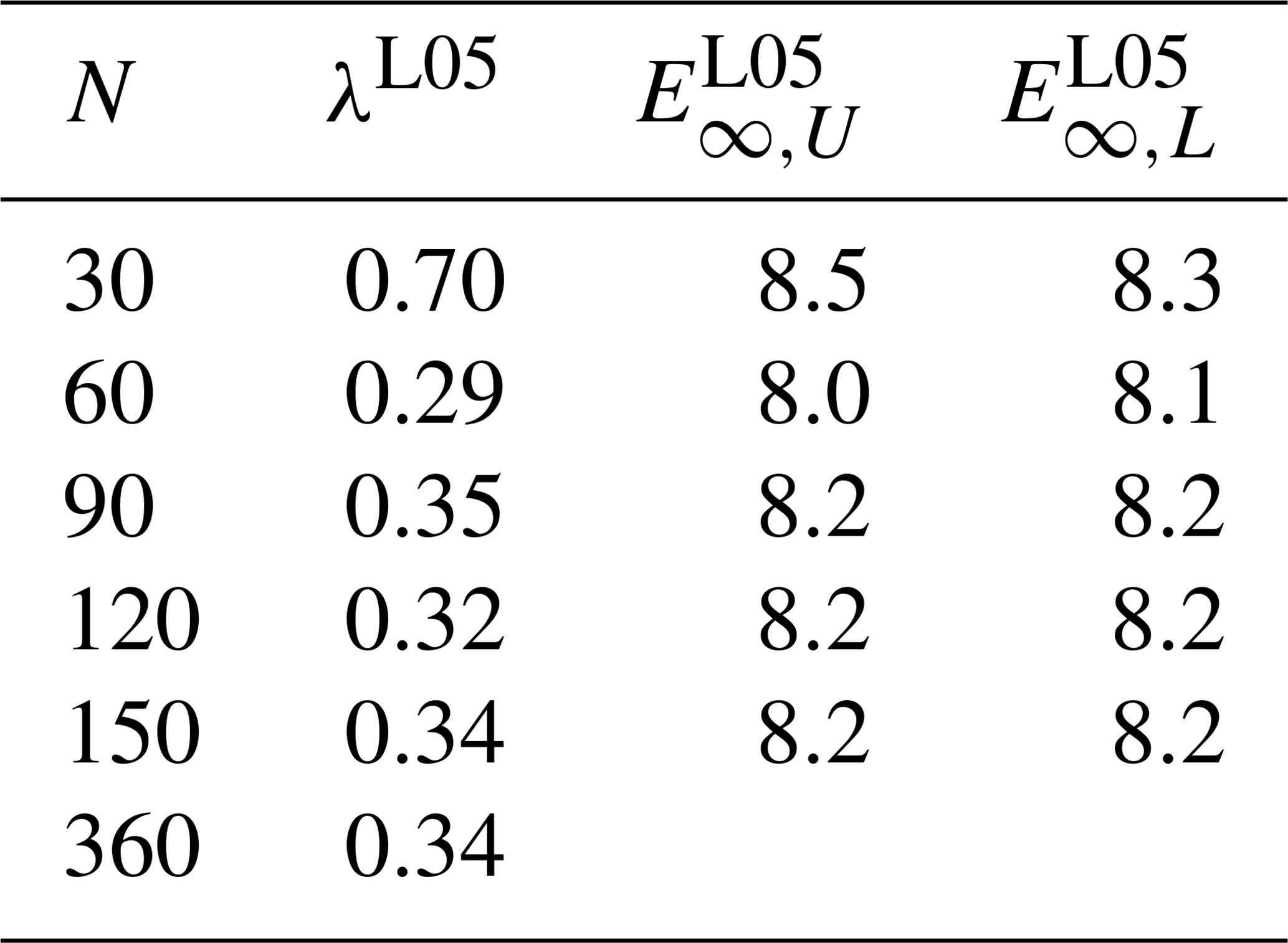
If L is even, denotes a modified summation, in which the first and last terms are to be divided by 2. If L is odd, denotes an ordinary summation. Generally, L is much smaller than N and if K is even and if L is odd. For comparison with predictability curves of the ECMWF forecasting system, we choose N=30, 60, 90, 120, 150, and 360. To keep a desirable number of main pressure highs and lows, Lorenz (2005) suggested to keep the ratio and therefore L=1, 2, 3, 4, 5, and 12. For even values of L we have J=1, 2, and 6, and for odd values of L we have J=0, 1, and 2. The parameter F=15 is selected as a compromise between a Lyapunov exponent that is too high (smaller F) and undesirable shorter waves (larger F). For this setting and by the method of numerical calculation (Sprott, 2006), the largest global Lyapunov exponents are calculated (Table 2). By the definition of Lorenz (1969): “A bounded dynamical system with a positive Lyapunov exponent is chaotic”. Because the value of the largest Lyapunov exponent is positive and the system under study is bounded, it is chaotic. Strictly speaking (Aligood et al., 1996), we also need to exclude the asymptotically periodic behavior, but such a task is impossible to fulfill for the numerical simulation. The choice of parameters F and time unit =5 d is made to obtain a similar value of the largest Lyapunov exponent as the ECMWF forecasting system.
To calculate predictability curves (Lorenz, 1996), arbitrary values of the variables Xn are chosen, and, using a fourth-order Runge–Kutta method with a time step Δt=0.05 or 6 h, they are integrated forward for 14 400 steps or 10 years. Final values X0,n, which should be free of transient effect, are the initial values of “reality”. Initial values of “prediction” are , where e0,n is the initial error and it is chosen randomly from a normal distribution ND(μ;σ), where μ=0 is mean and σ is the standard deviation, which is chosen from comparison with the ECMWF forecasting system. From X0,n and Eq. (2) is integrated forward for 37.5 d (K=150 steps). For upper-bound predictability curves, Xn and are chosen with the same number of variables (N=30, 60, 90, 120, 150). For lower-bound predictability curves, Xn is defined by X0,n and by Eq. (2) with N0=360 and by and by Eq. (2) with N=30, 60, 90, 120, and 150. The size of the model error is corrected by the difference of N for Xn and . If, for example, N=120 then Xn is compared with in each third point of N0. This method was presented by Lorenz (2005). Although not only resolution but also physical parameterization affects the deficiencies of the ECMWF system, which make it different from the real atmosphere, Buizza (2010) showed that a comparison of predictability curves of the ECMWF system calculated from differences of prediction and analysis as well as from two predictions of systems with different horizontal resolutions leads to the same overall conclusions. Despite the sub-differences mentioned by Buizza (2010), this method is sufficient for comparing the L05 system and the ECMWF forecasting system.
In each time step Δt of numerical integration N “real” and N “predicted” values are obtained. The size of the error at a given time for upper-bound predictability curves is , where and and for lower-bound predictability curves , where , (except for N0). (except for N0) is the location of the value for N=360, where for N=30, 60, 90, 120, and 150. The predictability curves of the ECMWF forecasting system, in this case, are obtained from annual averages of daily data. To simulate that, the number of runs M=400 is made. In each new run, initial values X0,n are the last values XK,n from the previous run. M⋅N values are obtained for each k. Final formulas of prediction errors that constitute predictability curves by calculation with arithmetic mean (A) are
Formulas to calculate prediction errors by geometric means (G) are
For an overview of the symbols see Table 1.
To calculate predictability curves for the ECMWF forecasting system (EFS) values of 500 hPa geopotential height are used. Data were obtained from ECMWF (Magnusson, 2018). Lower-bound predictability curves are calculated (Magnusson and Kallen, 2013) from 21 root mean squares over the Northern Hemisphere (20–90∘ N) obtained daily from 1 January 1986 to 31 December 2011. Means are differences between operational forecasts and analyses from ERA-Interim for a given day. Forecasts range from 0.5 d ago relative to the given day to 10 d ago, with time step 0.5 d. The difference between operational analysis and analysis from ERA-Interim is taken as the initial error. Upper-bound predictability curves are calculated (Magnusson and Kallen, 2013) from 27 root mean squares over the Northern Hemisphere (20–90∘) obtained daily from 1 January 1986 to 31 December 2011. Means are differences between two operational forecasts issued with a 1 d lag but that are valid on the same day. Specifically, the following differences are obtained for a given day (hours): 0–24, 6–30, 12–36, 18–42, 24–48, 30–54, 36–60, 42–66, 48-72, 54–78, 60–84, 66–90, 72–96, 78–102, 84–108, 90–114, 96–120, 108–132, 120–144, 132–156, 144–168, 156–180, 168–192, 180–204, 192–216, 204–228, and 216–240. Prediction errors constituting the predictability curves are calculated as annual averages of daily data. Detailed information about calculating predictability curves of the ECMWF forecasting system can be found in Lorenz (1982).
Table 1Description of symbols that indicate types of predictability curve, types of mean and systems for prediction error E, theoretically calculated limit error E∞, and parameters of error growth models α, β, p, and Elim (Eqs. 8–13).
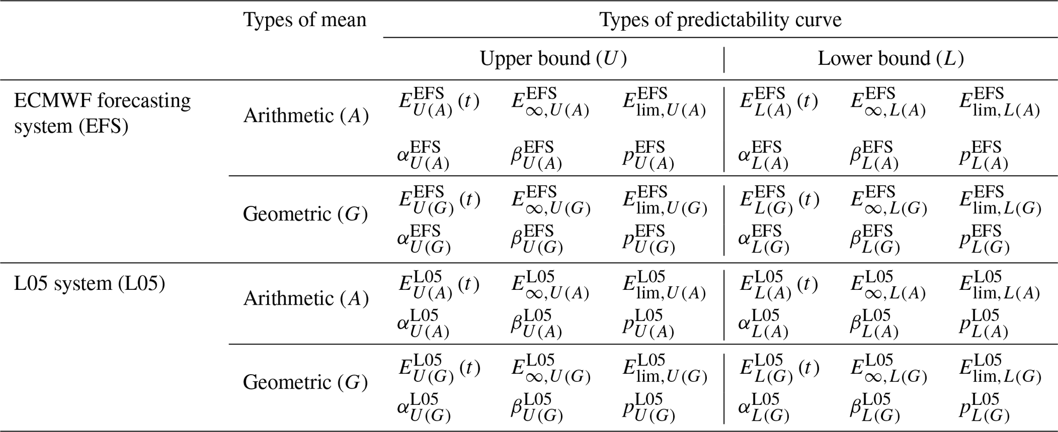
Table 2Values of the largest global Lyapunov exponents λL05 and limit values of predictability curves and for the displayed number of variables N of the L05 system.
Comparisons of model predictability curves are done through values normalized by the limit (saturated) errors (, . Because the maximum forecast time for the ECMWF forecasting system is 10 d, presented predictability curves do not reach their limit value. An independent measure of limit error can be calculated as
where is the time-averaged anomaly with respect to climate and is the time-averaged analysis anomaly with respect to climate. The climate is defined from ERA-Interim daily climatology. E∞,U and E∞,L differ if the ECMWF forecasting system does not sufficiently describe the variability of the atmosphere (model error). More information can be found in Simmons et al. (1995). Because it will be shown that values of limit error calculated by this method are not correct, predictability curves of the ECMWF forecasting system are normalized by values calculated by Eq. (15).
Predictability curves of the ECMWF (26 annual averages) and L05 systems are compared to find a setting of the L05 system (number of variables N, the size of the initial errors, preference of arithmetic or geometric mean) that gives the most similar progress of systems' predictability curves.
Predictability curves of the L05 system show negative growth for the first time step (6 h) but turn into an increase thereafter. At the second time step (12 h) values of predictability curves reach approximately the same values as they had initially. A possible explanation could be that initial errors set the initial state off the attractor and a decrease occurs because the first tendency is to get on the attractor (Brisch and Kantz, 2019). With an increase in average errors, chaotic behavior becomes dominant. Predictability curves of the ECMWF forecasting system do not exhibit this type of behavior. This may be because of larger time steps or methods of objective analysis. We aim to get the most similar predictability curves of both models, and therefore the first two time steps (up to 12 h) of the L05 model's predictability curves are filtered out.
A description of symbols that indicate the type of prediction error E in the text is provided in Table 1. Initial values and or equivalently standard deviations σ from a normal distribution ND(μ;σ) of the L05 system are calculated from a comparison of initial values of the ECMWF system (26 annual averages) that are normalized (ENorm) by limit (saturated) errors calculated by Eq. (15). Upper-bound predictability curves start for the ECMWF forecasting system on day 1 (the difference between 1 d prediction and the analysis), and therefore is calculated from predictability curves that are close on the first day: . Initial values for the L05 system are computed for N=60, 90, 120, and 150. Normalized predictability curves with N=30 exhibit different evolution compared to predictability curves of the ECMWF forecasting system, and they are not displayed. Initial prediction errors calculated by arithmetic and geometric mean as well as N=60, 90, 120, and 150 have the same values, and these values are in the interval , where lower values correspond to initial prediction errors of the ECMWF system from later years and higher values pertain to early years. For lower-bound predictability curves of the ECMWF forecasting system, the initial error is computed as a difference between analysis from the operational forecasting system and analysis from ERA-Interim. Initial errors of the L05 system are calculated as and , where lower values correspond to initial prediction errors of the ECMWF system from later years and higher values pertain to early years. Initial values are the same for all N as well as arithmetic and geometric mean.
Predictability curves calculated by arithmetic and geometric mean show a significant difference for the L05 system (all N), which agrees with Ruiqiang and Jianping (2011), and a minor difference for the ECMWF forecasting system. For the L05 system and upper- and lower-bound predictability curves, the maximal difference is between 6.5 % and 10.5 % of or , and these maximal values occur between 5 and 9 d of forecast length. For the ECMWF forecasting system and upper- and lower-bound predictability curves, the maximal difference is 2 % of or , and these maximal values occur at the end of the forecast length (10 d). The choice of the averaging method does not significantly change the evolution of the ECMWF forecasting system's predictability curves, and it does not change values of parameters of the approximations. For the L05 system, the choice of averaging method is significant, and it changes values of the parameters. The reason for this sensitivity can be found in the spread of values that are used for averaging. For the ECMWF forecasting system, the values are closer to each other than for the L05 system, and from the definition of means, it leads to the aforementioned difference. Calculating predictability curves by arithmetic and geometric mean, although it does not affect predictability curves of the ECMWF forecasting system, is mentioned because it affects the calculation of predictability curves of the L05 system, and this then affects the comparison of predictability curves, which is important for recalculation of error growth models' parameters for the ECMWF forecast system.
The comparison of predictability curves is done with given initial values. Predictability curves of the ECMWF forecasting system are normalized by or (Fig. 7, black full curves) and for the L05 system by and displayed in Table 2 (for a description of the symbols see Table 1). For the L05 system predictability curves are calculated with N=60, 90, 120, and 150 variables and by arithmetic and geometric mean (for lower-bound predictability curves this sets different values of the model error). For the ECMWF forecasting system only arithmetic mean is used.
A comparison of lower-bound predictability curves (Fig. 2) shows the most similar predictability curves of the ECMWF forecasting system and the L05 system for the L05 system calculated by arithmetic mean with N=90 (the fact that this would mean unrealistic values of the model error for the ECMWF forecasting system is further discussed). For upper-bound predictability curves (Fig. 1), predictability curves for the L05 system with N=90 are the most similar to the year 1999 for predictability curves of the L05 system calculated by geometric mean and after 1999 by the arithmetic mean.
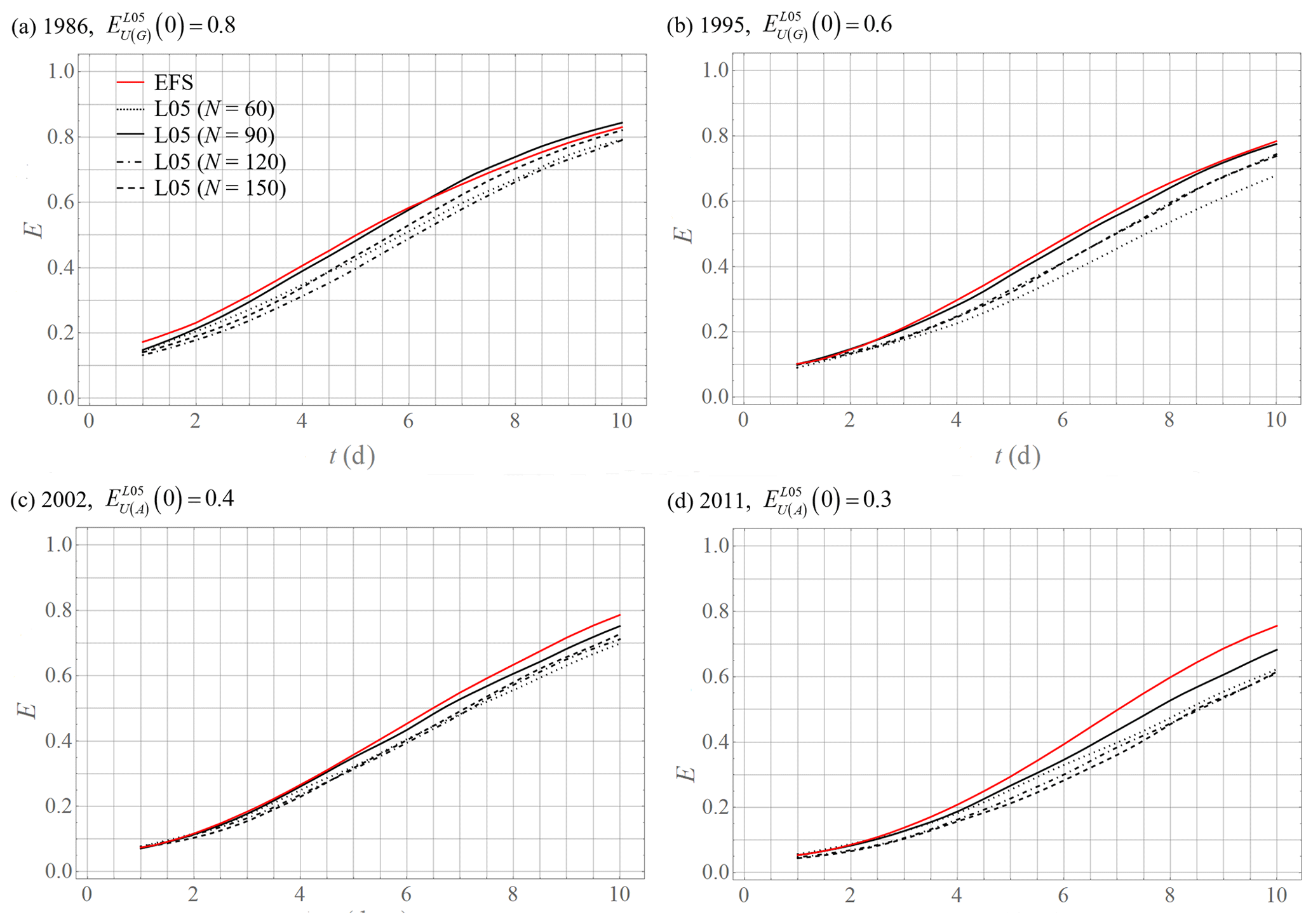
Figure 1Comparison of upper-bound predictability curves Enorm,U of the ECMWF forecasting system normalized by (Eq. 15) (EFS; annual arithmetic means, representative samples from 1986–2011) and the L05 system normalized by (Table 2) (L05; geometric means 1986–1999, arithmetic means 2000–2011).
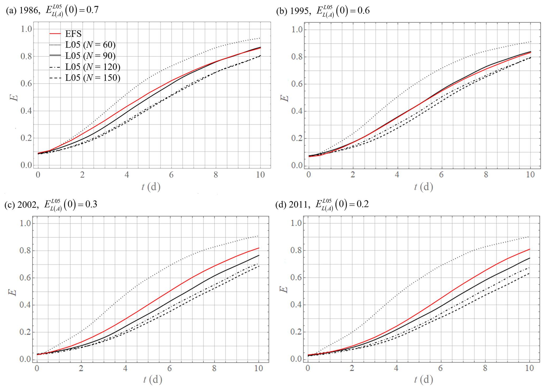
Figure 2Comparison of lower-bound predictability curves Enorm,L of the ECMWF forecasting system normalized by (Eq. 15) (EFS; annual arithmetic means, representative samples from1986–2011) and the L05 system normalized by (Table 2) (L05; arithmetic mean).
Parameters of error growth models are the Lyapunov exponent, model error, and limit error. They are estimated from approximations of predictability curves or differences of predictability curves , where t is time and Δt=0.25 d (Figs. 3 and 4). Error growth models considered here are
where parameters of Tm are α=2a, , and
where parameters of Tmβ are , , and . E is an average forecast error. t represents time, α is the estimate of the Lyapunov exponent λ, β is the parameter of model error ( when E=0), Elim is the limit (saturated) value of E (value of E when , theoretically E∞; Figs. 3 and 4), and p, A, B, a, and b are parameters.
The calculation is done for the ECMWF forecasting system (26 annual averages) and the L05 system (N=90) for arithmetic (A) and geometric (G) means, upper-bound predictability curves (U), and lower-bound predictability curves (L). See Tables 3 and 4 for root mean square (rms) values of parameters , , , and that are calculated over all initial errors used for the L05 system and all calculated years for the ECMWF forecasting system.
Table 3The rms values calculated over all initial errors used for the L05 system (N=90) and over all years for the ECMWF forecasting system of parameters and (for description see Table 1).

Table 4The rms values calculated over all initial errors used for the L05 system (N=90) and over all years for the ECMWF forecasting system of parameters and (for description see Table 1).
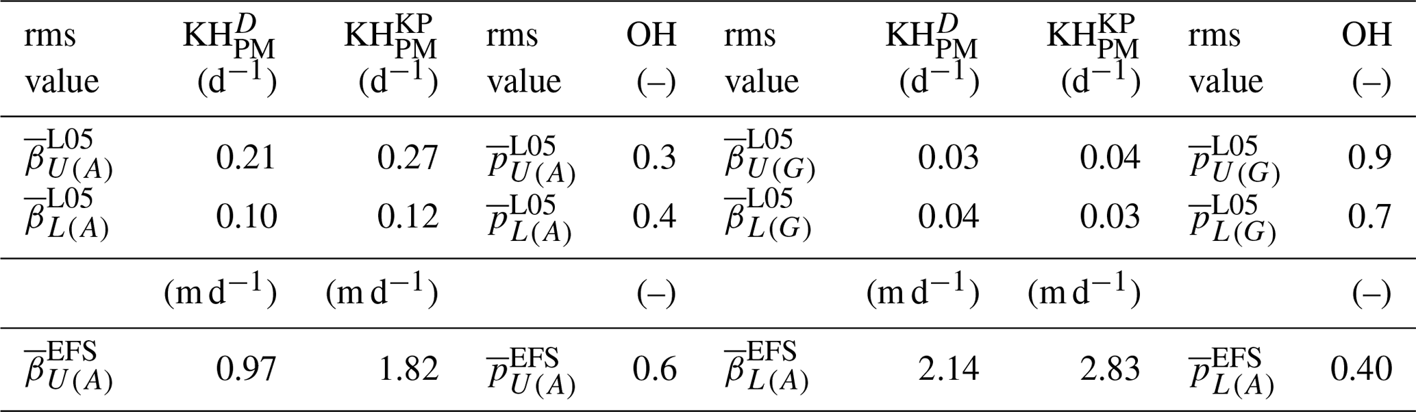
The average values of parameters and are higher for the lower-bound predictability curves than for the upper-bound predictability curves. Upper-bound predictability curves should not include model error (theoretically β=0), but from Table 4 it can be seen that for the L05 system (arithmetic mean) the values are even higher than for the lower-bound predictability curves. For the ECMWF forecasting system the values of are higher for lower-bound predictability curves, which is theoretically more acceptable, but is not zero for the upper-bound predictability curves. A possible explanation can be the sensitivity to correct approximation (cases with higher β have lower α), but this cannot fully explain the discrepancy. For the values of upper- and lower-bound predictability curves are similar to each other (L05 system and ECMWF forecasting system).
There are significant differences of parameters , , , and between predictability curves calculated by arithmetic and geometric mean for the L05 system (for the ECMWF forecasting system only arithmetic mean is presented). The most significant differences are detected for and ; for values are closer to zero for geometric mean and values of predictability curves calculated by arithmetic mean are 2 or 3 times higher. Values of parameter are closer to for geometric mean. This means that differences of predictability curves calculated by geometric mean have a shape that is close to a symmetric parabola (for example, Fig. 3a), but for the arithmetic mean the parabolic shape is skewed to the left (for example, Fig. 3c).
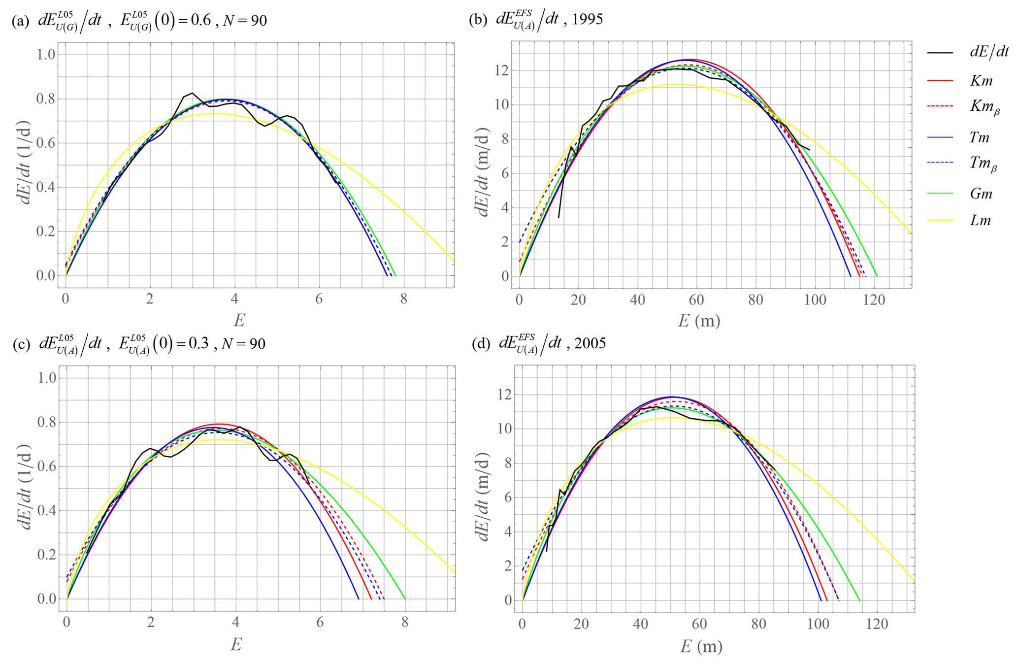
Figure 3Approximations of differences of upper-bound predictability curves (representative samples). (a, b) The most similar predictability curves in the year 1995 of the ECMWF forecasting system. (c, d) The most similar predictability curves in the year 2005 of the ECMWF forecasting system. Parameters from Tm used in Km (blue) and parameters from Tmβ used in Kmβ (blue dashed).
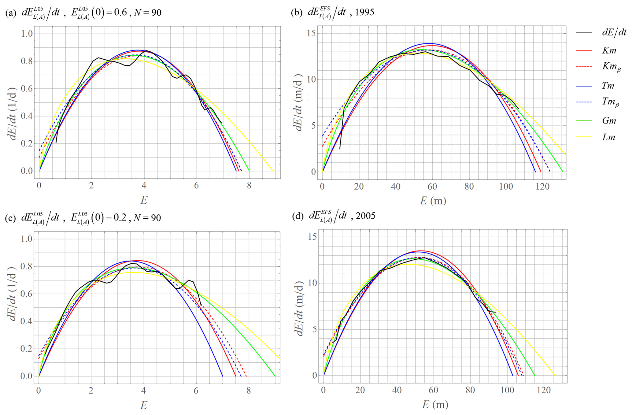
Figure 4Approximations of differences of lower-bound predictability curves (representative samples). (a, b) The most similar predictability curves in the year 1995 of the ECMWF forecasting system. (c, d) The most similar predictability curves in the year 2005 of the ECMWF forecasting system. Tm displays parameters from Tm used in Km, and Tmβ displays parameters from Tmβ used in Kmβ.
Note that the description of symbols that indicate the type of parameters of error growth models α, β, p, and Elim in the text is provided in Table 1. The Lyapunov exponent of the ECMWF forecasting system is recalculated by the formula
where αEFS and αL05 are parameters of error growth models and λL05=0.35 d−1. The formula (Eq. 14) is based on the assumption that if normalized predictability curves of the L05 system and the ECMWF forecasting system are similar, then the differences between true values of the largest global Lyapunov exponents (λEFS, λL05) and values determined from error growth models (αEFS, αL05) are similar (). Similarity of differences λ−α allows us to estimate the largest global Lyapunov exponents of the ECMWF forecasting system. For upper-bound predictability curves (the L05 system with N=90 to the year 1999 calculated by geometric mean and after 1999 by arithmetic mean), the average value over all error growth models is in the range 〈0.33;0.41〉 d−1 (Fig. 5a). Lm is not used because this error growth model is not sufficient to approximate predictability curves. Root mean square errors (RMSEs) of are mostly about 0.01 d−1 only in the years 1991, 1995, and 1997; a 1999 RMSE is about 0.02 d−1. For comparison, RMSEs of are in the range 〈0.02;0.07〉 d−1 (Fig. 5a). For lower-bound predictability curves (the L05 system with N=90 calculated by arithmetic mean), the average value over all error growth models is in the range 〈0.32;0.41〉 d−1 (Fig. 5b). RMSEs of are in the range 〈0.01;0.02〉 d−1. For comparison, RMSEs of are in the range 〈0.03;0.07〉 d−1 (Fig. 5b). The average value over upper- and lower-bound predictability curves is shown in Fig. 6, and RMSEs of are mostly about 0.01 d−1. Low values of RMSEs of compared to RMSEs of and similar values of for upper- and lower-bound predictability curves (low values of RMSEs of ) prove the validity of . Values of and are generally closer to parameters αEFS of Kmβ, Tmβ, and Gm than to αEFS of Km, Tm, and Lm, but none of the error growth models approximate (Fig. 6).
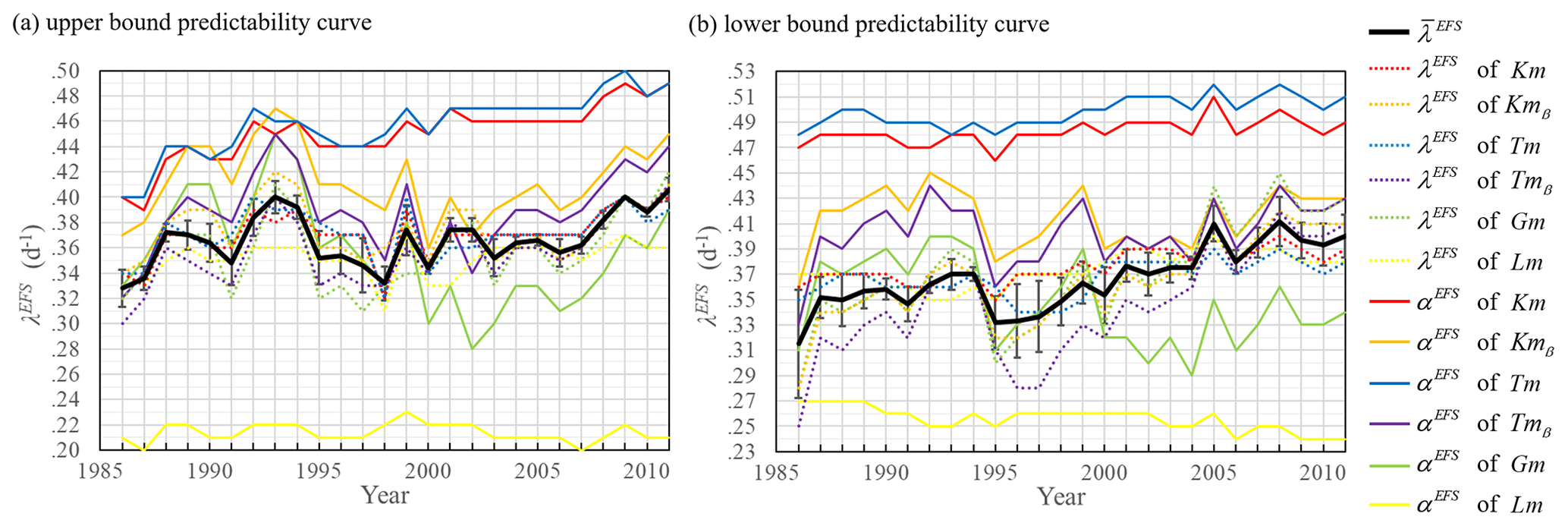
Figure 5Lyapunov exponents λEFS of the ECMWF forecasting system calculated by Eq. (14) and parameters αEFS of error growth models for (a) upper- and (b) lower-bound predictability curves. is the average value over all error growth models.
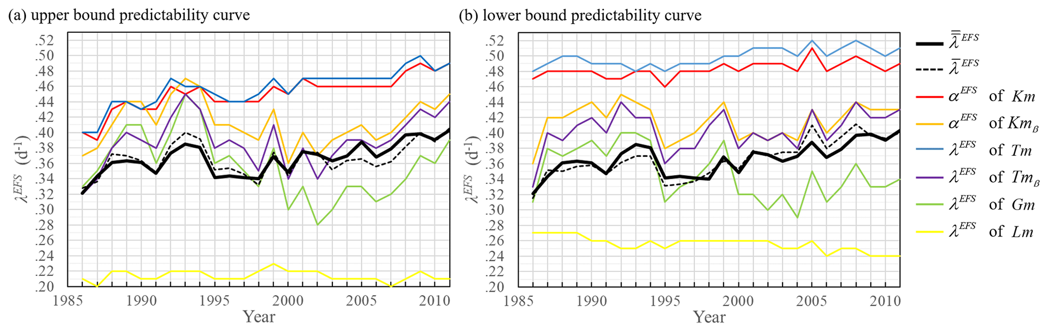
Figure 6Average values over upper- and lower-bound predictability curves of Lyapunov exponents (black, solid), average values (black dashed) for (a) upper- and (b) lower-bound predictability curves of the ECMWF forecasting system calculated by Eq. (14), and parameters αEFS of error growth model for (a) upper- and (b) lower-bound predictability curves of the ECMWF forecasting system.
New limit values are calculated from the error growth models by the formula
where and are values from error growth models and . As in calculating λEFS, Eq. (15) is based on the assumption that if normalized predictability curves of the L05 system and the ECMWF forecasting system are similar, then the differences between true limit values (, ) and values determined from error growth models (, ) are similar. In this case, however, only normalized values can be compared:
Similarity of normalized differences () allows us to estimate new limit values of the ECMWF forecasting system. For upper-bound predictability curves (the L05 system with N=90), the average value over all error growth models is in the range 〈96;133〉 m (Fig. 7a). Lm is not used because this error growth model is not sufficient to approximate predictability curves. RMSEs of are mostly about 1 m only in the years 1987, 1988, 1995, 1997, and 2003, and in 2011 it is about 2 m. For comparison, RMSEs of are in the range 〈2;6〉 m (Fig. 7a). For lower-bound predictability curves (the L05 system with N=90 calculated by arithmetic mean), the average value over all error growth models is in the range 〈114;134〉 m (Fig. 7b). Lm is not used because this error growth model is not sufficient to approximate predictability curves. RMSEs of are mostly 3 m, and after the year 2004, they are 4 m. RMSEs of are in the range 〈3;6〉 m (Fig. 7b). Lower values of RMSEs of and calculated by Eq. (15) compared to RMSEs of and prove the validity of and .
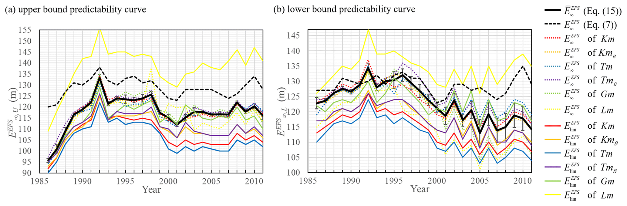
Figure 7Limit values of the ECMWF forecasting system calculated by Eq. (15) and parameters of error growth models for (a) upper- and (b) lower-bound predictability curves. (Eq. 15) is the average value over all error growth models, and (Eq. 7) represents limit values calculated by Eq. (7).
The argument that favors calculated by Eq. (15) (Fig. 7, black full curves) instead of calculated by Eq. (7) (Fig. 7, black dashed curves) is based on the parameter of model error β. The most similar predictability curves of the L05 system and the ECMWF forecasting system with calculated by Eq. (15) are found for the L05 system with N=90 (for lower-bound predictability curves calculated by arithmetic mean and for upper-bound predictability curves calculated by geometric mean to 1999 and after by arithmetic mean). The most similar predictability curves of the L05 system and the ECMWF forecasting system with calculated by Eq. (7) are found for the L05 system with N=90 by the arithmetic mean for upper- and lower-bound predictability curves. It means that if the comparison is valid and model error is constant for the L05 system (same number of variables over years in the L05 system means constant model error over years), it must also be constant for the ECMWF forecasting system, but the calculation of parameters shows a decreasing trend with increasing time (Fig. 8b). But parameters have nonzero values (Fig. 8a) that are close to for some years, and that is inconsistent with the theoretical expectation that upper-bound predictability curves should be without model error; therefore, β should be 0 m d−1. This inconsistency can be solved by the new definition of the model error. From Fig. 6 it can be seen that a closer value of αEFS to for αEFS is approximated from error growth models Kmβ, Tmβ, and Gm than for αEFS approximated from error growth models Km, Tm, and Lm. Gm has parameter p that defines skewness of the originally parabolic shape of the difference of predictability curves. p=1 pertains to symmetrical parabolic shape (Gm becomes Km) and p=0 means the greatest skewness to the left (Gm becomes Lm). Parameters β also skew the originally parabolic shape (Figs. 3 and 4). The model error can be seen as a difference between skewness of upper- and lower-bound predictability curves, and the new definition of model error would be
Results (Fig. 9a) show good agreement for (Eq. 16) calculated from Kmβ and Tmβ, a decreasing trend of with increasing time for predictability curves with calculated by Eq. (15), and almost constant values of with increasing years (slight decrease can be due to the error of approximations) for predictability curves with calculated by Eq. (7). There is also good agreement with trends of |pL−pU| (Fig. 9b). Because constant values of βL−U for predictability curves with calculated by Eq. (7) are not theoretically possible, predictability curves with calculated by Eq. (15) are favored. The reason for the decreasing trend of , which is found for predictability curves of the L05 system with N=90 that are the most similar to predictability curves of the ECMWF forecasting system normalized by calculated by Eq. (15), is that they are partly calculated by geometric and partly by the arithmetic mean.
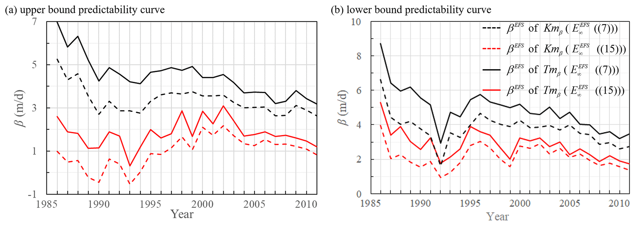
Figure 8Parameters βEFS (a) for upper-bound predictability curves and (b) for lower-bound predictability curves . Black curves represent βEFS approximated from predictability curves with calculated by Eq. (7), red curves pertain to βEFS approximated from predictability curves with calculated by Eq. (15), full curves correspond to βEFS calculated from Tmβ, and dashed curves correspond to βEFS calculated from Kmβ.
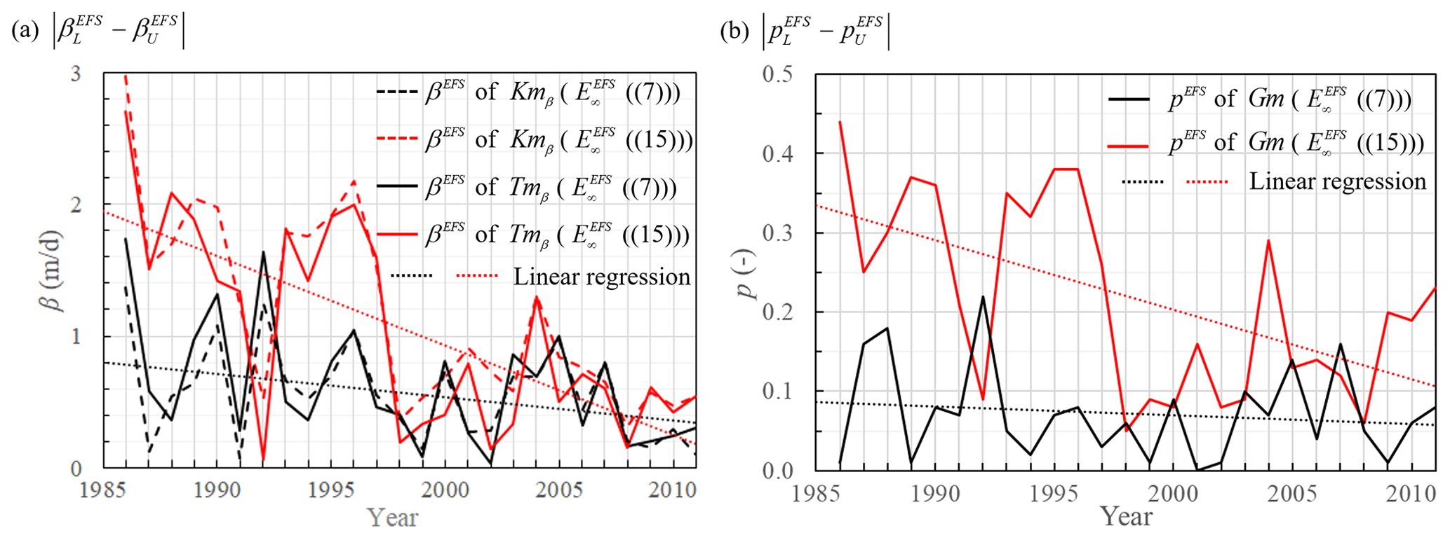
Figure 9Absolute values of differences of parameters (a) and (b) between lower- and upper-bound predictability curves. For the notation see Fig. 8.
These arguments are taken as proof of the validity of and calculated by Eq. (15). The reason for the overestimation of calculated by Eq. (7) (Fig. 7) can be found in the multiscale behavior of weather. If some events are predictable on a timescale longer than 10 d (for example, long-lived anomalies in sea surface temperature or soil moisture), then they would not be captured by medium-range weather forecast (Simmons et al., 1995; Brisch and Kantz, 2019). It is also possible that the overestimation is due to the different source of data used for calculation of by Eqs. (7) and (15). For calculated by Eq. (7) only data from ERA-Interim (Janoušek, 2011) are used, but for calculated by Eq. (15) data from the operational forecast are employed.
At the end of this section, it is important to remind the readers about the importance of the correct values of the parameters. Zhang et al. (2019) used Kmβ in the ECMWF forecasting system to estimate the influence of different spatiotemporal scales with the parameter β newly representing the intrinsic upscale error growth and propagation from small scales and α representing synoptic-scale error growth. The results of our analysis support this approach by the new definition of model error (Eq. 16) and by showing the errors of approximations for individual error growth models.
The values of error growth models' (Eqs. 8–13) parameters that approximate predictability curves and their differences (Figs. 3 and 4) in the ECMWF forecast system (Tables 3 and 4) were recalculated. This is based on similarities of normalized upper- and lower-bound predictability curves (Figs. 1 and 2) of the ECMWF forecasting system (annual arithmetic mean of geopotential heights of 500 hPa from years 1986–2011) and the L05 system (N=90, arithmetic mean for lower-bound predictability curves; geometric mean up to 1999 and arithmetic mean after 1999 for upper-bound predictability curves). It is also based on knowledge of the largest Lyapunov exponent (λ=0.35 d−1) and the limit value of the predictability curve (E∞=8.2) of the L05 system.
Lyapunov exponents of the ECMWF forecasting system were recalculated by Eq. (14). The average value over all error growth models for upper-bound predictability is in the range 〈0.33;0.41〉 d−1 (Fig. 5a) and RMSEs are mostly about 0.01 d−1. For lower-bound predictability curves the average value over all error growth models is in the range 〈0.32;0.41〉 d−1 (Fig. 5b). RMSEs are in the range 〈0.01;0.02〉 d−1. The average value over upper- and lower-bound predictability curves is shown in Fig. 6 and RMSEs are mostly about 0.01 d−1. Values of the Lyapunov exponent are generally closer to parameters αEFS of Kmβ, Tmβ, and Gm than to αEFS of Km, Tm, and Lm (Fig. 6).
New limit values were calculated from the error growth models by Eq. (15). For upper-bound predictability curves, the average value over all error growth models is in the range 〈96;133〉 m (Fig. 7a) and RMSEs are mostly about 1 m. For lower-bound predictability curves the average value over all error growth models is in the range 〈114;134〉 m (Fig. 7b) and RMSEs are mostly 3 m.
The argument that favors limit values calculated by Eq. (15) (Fig. 7, black full curves) instead of limit values calculated by Eq. (7) (Fig. 7, black dashed curves) is based on the new definition of model error (Eq. 16) that shows a decreasing trend with increasing years for predictability curves with limit values calculated by Eq. (15) and an almost constant trend with increasing time (slight decrease can be due to the error of approximations) for predictability curves with limit values calculated by Eq. (7), which is theoretically impossible (Fig. 9a). This new model error calculated as a difference of model error parameters between the upper- (Fig. 8a) and lower-bound (Fig. 8b) predictability curves supports model error parameters calculated for upper-bound predictability curves that are used to represent the intrinsic upscale error growth and propagation from small scales (Zhang et al., 2019).
The ECMWF forecasting system dataset was obtained from the personal repository of Linus Magnusson (Magnusson, 2013). The L05 system dataset, products from the ECMWF forecasting system dataset, codes, and figures were conducted in Wolfram Mathematica, and they are permanently stored at https://doi.org/10.17605/OSF.IO/CEK32 (Bednář, 2020).
HB proposed the idea, carried out the experiments, and wrote the paper. AR and JM supervised the study and co-authored the paper.
The contact author has declared that neither they nor their co-authors have any competing interests.
Publisher's note: Copernicus Publications remains neutral with regard to jurisdictional claims in published maps and institutional affiliations.
The authors are grateful to Linus Magnusson for offering the dataset.
This research has been supported by the Czech Science Foundation (grant no. 19-16066S).
This paper was edited by Richard Neale and reviewed by two anonymous referees.
Alligood, K. T., Sauer, T. D., and Yorke, J. A.: Chaos an Introduction to Dynamical System, Springer, New York, USA, 1996.
Bednář, H.: Recalculation of error growth models’ parameters for the ECMWF forecast system, OSF [code and data set] https://doi.org/10.17605/OSF.IO/CEK32, 2020.
Bengtsson, L. K., Magnusson, L., and Kallen, E.: Independent Estimations of the Asymptotic Variability in an Ensemble Forecast System, Mon. Weather Rev., 136, 4105–4112, https://doi.org/10.1175/2008MWR2526.1, 2008.
Brisch, J. and Kantz, H.: Power law error growth in multi-hierarchical chaotic system-a dynamical mechanism for finite prediction horizon, New J. Phys., 21, 1–7, https://doi.org/10.1088/1367-3630/ab3b4c, 2019.
Buizza, R.: Horizontal Resolution Impact on Short- and Long-range Forecast Error, Q. J. Roy. Meteorol. Soc., 136, 1020–1035, https://doi.org/10.1002/qj.613, 2010.
Dalcher, A. and Kalney, E.: Error growth and predictability in operational ECMWF analyses, Tellus A, 39, 474–491, https://doi.org/10.1111/j.1600-0870.1987.tb00322.x, 1987.
Froude, L. S., Bengtsson, L., and Hodges, K. I.: Atmospheric Predictability Revised, Tellus A, 63, 1–13, https://doi.org/10.3402/tellusa.v65i0.19022, 2013
Janoušek, M.: ERA-Interim daily climatology, https://confluence.ecmwf.int/download/attachments/24316422/daily_climatology_description.pdf (last access: 20 October 2018), 2011.
Lorenz, E. N.: Deterministic nonperiodic flow, J. Atmos. Sci., 20, 130–141, https://doi.org/10.1175/1520-0469(1963)020<0130:DNF>2.0.CO;2, 1963.
Lorenz, E. N.: Atmospheric predictability as revealed by naturally occurring analogs, J. Atmos. Sci., 26, 636–646, https://doi.org/10.1175/1520-0469(1969)26<636:APARBN>2.0.CO;2, 1969.
Lorenz, E. N.: Atmospheric predictability experiments with a large numerical model, Tellus, 34, 505–513, https://doi.org/10.1111/j.2153-3490.1982.tb01839.x, 1982.
Lorenz, E. N.: Predictability: a problem partly solved, in: Predictability of Weather and Climate, edited by: Palmer, T. and Hagedorn, R., Cambridge University Press, Cambridge, UK, 1–18, https://doi.org/10.1017/CBO9780511617652.004, 1996.
Lorenz, E. N.: Designing chaotic models, J. Atmos. Sci., 62, 1574–1587, https://doi.org/10.1175/JAS3430.1, 2005.
Magnusson, L.: Factors Influencing Skill Improvements in the ECMWF Forecasting System, available from personal repository: linus.magnusson@ecmwf.int [data set] (last access: 13 November 2018), 2013.
Magnusson, L. and Kallen, E.: Factors Influencing Skill Improvements in the ECMWF Forecasting System, Mon. Weather Rev., 141, 3142–3153, https://doi.org/10.1175/MWR-D-12-00318.1, 2013.
Ruiqiang, D. and Jianping, L.: Comparisons of Two Ensemble Mean Methods in Measuring the Average Error Growth and the Predictability, Acta Meteor. Sin., 25, 395–404, https://doi.org/10.1007/s13351-011-0401-4, 2011.
Savijarvi, H.: Error Growth in a Large Numerical Forecast System, Mon. Weather Rev., 123, 212–221, https://doi.org/10.1175/1520-0493(1995)123<0212:EGIALN>2.0.CO;2, 1995.
Simmons, A. J., Mureau, R., and Petroliagis, T.: Error growth and estimates of predictability from the ECMWF forecasting system, Q. J. Roy. Meteorol. Soc., 121, 1739–1771, https://doi.org/10.1002/qj.49712152711, 1995.
Sprott, J. C.: Chaos and Time-series Analysis, Oxford university press, New York, USA, 2006.
Stroe, R. and Royer, J. F.: Comparison of Different Error Growth Formulas and Predictability Estimation in Numerical Extended-range Forecasts, Ann. Geophys., 11, 296–316, 1993.
Stroe, R. and Royer, J. F.: An Improved Formula to Describe Error Growth in Meteorological Models, in: Predictability and Nonlinear Modelling in Natural Sciences and Economics, edited by: Grasman, J. and van Straten, G., Kluwer Academic Publishers, Wageningen, NE, 45–56, 1994.
Trevisan, A.: Impact of Transient Error Growth on Global Average Predictability Measure, J. Atmos. Sci., 50, 1016–1028, https://doi.org/10.1175/1520-0469(1993)050<1016:IOTEGO>2.0.CO;2, 1993.
Trevisan, A., MalgguziI, P., and Fantini, M.: On Lorenz's law for the growth of large and small errors in the atmosphere. J. Atmos. Sci., 49, 713–719, https://doi.org/10.1175/1520-0469(1992)049<0713:OLLFTG>2.0.CO;2, 1992.
Žagar, N., Buizza, R., and Tribbia, J.: A Three-Dimensional Multivariate Modal Analysis of Atmospheric Predictability with Application to the ECMWF Ensemble, J. Atmos. Sci., 72, 4423–4444, https://doi.org/10.1175/JAS-D-15-0061.1, 2015.
Žagar, N., Horvat, M., Zaplotnik, Ž., and Magnusson, L.: Scale-dependent Estimates of the Growth of Forecast Uncertainties in Global Prediction System, Tellus A, 69, 1–14, https://doi.org/10.1080/16000870.2017.1287492, 2017.
Zhang, F., Sun, Q., Magnusson, L., Buizza, R., Lin, S. H., Chen, J. H., and Emanuel, K.: What is the Predictability Limit of Multilatitude Weather, J. Atmos. Sci., 76, 1077–1091, https://doi.org/10.1175/JAS-D-18-0269.1, 2019.
- Abstract
- Introduction
- Experimental setting
- Calculation of predictability curves
- Comparison of predictability curves
- Estimation of parameters
- Discussion
- Conclusions
- Code and data availability
- Author contributions
- Competing interests
- Disclaimer
- Acknowledgements
- Financial support
- Review statement
- References