the Creative Commons Attribution 4.0 License.
the Creative Commons Attribution 4.0 License.
 | 30 Nov 2021
STEMMUS-UEB v1.0.0: integrated modeling of snowpack and soil water and energy transfer with three complexity levels of soil physical processes
Lianyu Yu
Zhongbo Su
A snowpack has a profound effect on the hydrology and surface energy conditions of an area through its effects on surface albedo and roughness and its insulating properties. The modeling of a snowpack, soil water dynamics, and the coupling of the snowpack and underlying soil layer has been widely reported. However, the coupled liquid–vapor–air flow mechanisms considering the snowpack effect have not been investigated in detail. In this study, we incorporated the snowpack effect (Utah energy balance snowpack model, UEB) into a common modeling framework (Simultaneous Transfer of Energy, Mass, and Momentum in Unsaturated Soils with Freeze-Thaw, STEMMUS-FT), i.e., STEMMUS-UEB. It considers soil water and energy transfer physics with three complexity levels (basic coupled, advanced coupled water and heat transfer, and finally explicit consideration of airflow, termed BCD, ACD, and ACD-air, respectively). We then utilized in situ observations and numerical experiments to investigate the effect of snowpack on soil moisture and heat transfer with the abovementioned model complexities. Results indicated that the proposed model with snowpack can reproduce the abrupt increase of surface albedo after precipitation events while this was not the case for the model without snowpack. The BCD model tended to overestimate the land surface latent heat flux (LE). Such overestimations were largely reduced by ACD and ACD-air models. Compared with the simulations considering snowpack, there is less LE from no-snow simulations due to the neglect of snow sublimation. The enhancement of LE was found after winter precipitation events, which is sourced from the surface ice sublimation, snow sublimation, and increased surface soil moisture. The relative role of the mentioned three sources depends on the timing and magnitude of precipitation and the pre-precipitation soil hydrothermal regimes. The simple BCD model cannot provide a realistic partition of mass transfer flux. The ACD model, with its physical consideration of vapor flow, thermal effect on water flow, and snowpack, can identify the relative contributions of different components (e.g., thermal or isothermal liquid and vapor flow) to the total mass transfer fluxes. With the ACD-air model, the relative contribution of each component (mainly the isothermal liquid and vapor flows) to the mass transfer was significantly altered during the soil thawing period. It was found that the snowpack affects not only the soil surface moisture conditions (surface ice and soil water content in the liquid phase) and energy-related states (albedo, LE) but also the transfer patterns of subsurface soil liquid and vapor flow.
- Article
(8918 KB) - Full-text XML
-
Supplement
(6056 KB) - BibTeX
- EndNote


In cold regions, the snowpack has a profound effect on hydrology and surface energy through its change of surface albedo, roughness, and insulating properties (Boone and Etchevers, 2001; Zhang, 2005). In contrast to rainfall, the melted snowfall enters the soil with a significant lag in time, and a large and sudden outflow or runoff may be produced because of the snowmelt effect. The heat-insulating property of snow cover also provides a buffer layer to reduce the magnitude of the underlying subsurface temperature variations and thus markedly affects the thickness of the active layer in cold regions. The effect of snow cover on the subsurface soils has been studied and reviewed (e.g., Zhang, 2005; Hrbáček et al., 2016). For instance, snow cover can act as an insulator between atmosphere and soil with its low thermal conductivity (Zhang, 2005; Hrbáček et al., 2016). The snowmelt functions as the energy sink via the absorption of heat due to phase change (Zhang, 2005). Yi et al. (2015) investigated the seasonal snow cover effect on the soil freezing and thawing process and its related carbon implications. Such studies mainly focus on the thermal effect of snowpack on the frozen soils. However, the effect of snowpack on the soil water and vapor transfer process is rarely reported (Hagedorn et al., 2007; Iwata et al., 2010; Domine et al., 2019).
Table 1Brief overview of current soil–snow modeling efforts.
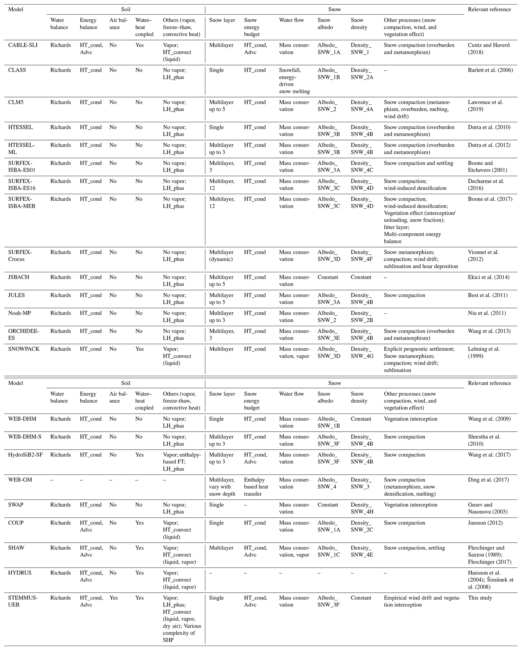
The abbreviations used in the table are as follows: HT_cond, heat conduction; Advc, advection; LH_phas, latent heat due to phase change; HT_Convect, convective heat due to liquid; SHP, soil physical process; Albedo_SNW_1A, snow albedo 1A, a function of snow age; Albedo_SNW_1B, snow albedo 1B, empirical function considering dry and wet states; Albedo_SNW_1C, snow albedo 1C, a function of extinction coefficient, grain size, and solar zenith angle; Albedo_SNW_2, snow albedo 2, a two-stream radiative transfer solution considering snow aging, solar zenith angle, optical parameters, and impurity; Albedo_SNW_3A, snow albedo 3A, prognostic snow albedo considering aging effect; Albedo_SNW_3B, snow albedo 3B, prognostic snow albedo considering aging effect and vegetation type dependent; Albedo_SNW_3C, snow albedo 3C, prognostic snow albedo considering aging and optical diameter; Albedo_SNW_3D, snow albedo 3D, prognostic snow albedo considering age and microstructure; Albedo_SNW_3E, snow albedo 3E, prognostic snow albedo considering aging effect and dry and wet states; Albedo_SNW_3F, snow albedo 3F, prognostic snow albedo considering aging effect and solar zenith angle; Albedo_SNW_4, snow albedo 4, diagnostic snow albedo considering snow aging, sleet and snowfall fraction, grain diameter, cloud fraction, and solar elevation effect; Density_SNW_1, snow density 1 relying on in situ measurements; Density_SNW_2A, snow density 2A, a function of air temperature; Density_SNW_2B, snow density 2B, a function of extinction coefficient and grain-size; Density_SNW_2C, snow density 2C, a function of old (densification), newly fallen (air temperature) snow pack density, and snow depth; Density_SNW_3, snow density 3, diagnostic density considering wet-bulb temperature; Density_SNW_4A, snow density 4A, prognostic density considering temperature, wind effect, snow compaction, and water and ice states; Density_SNW_4B, snow density 4B, prognostic density considering overburden and thermal metamorphisms; Density_SNW_4C, snow density 4C, prognostic snow density considering snow compaction and settling; Density_SNW_4D, snow density 4D, prognostic snow density considering snow compaction and wind-induced densification; Density_SNW_4E, snow density 4E, prognostic snow density considering snow compaction, settling, and vapor transfer; Density_SNW_4F, snow density 4F, prognostic density, a function of wind speed and air temperature; Density_SNW_4G, Snow density 4G, prognostic density, a function of stress state and microstructure; Density_SNW_4H, Snow density 4H, prognostic density considering snow temperature.
A great amount of effort has been made to better reproduce the snowpack characteristic and its effects in models. Initially, snowpack dynamics were expressed as a simple function of temperature. Nevertheless, these empirical relations have limited applications in complex climate conditions (Pimentel et al., 2015). Many physically based models for the mass and energy balance in the snowpack have been developed for their coupling with hydrological models or atmospheric models. Boone and Etchevers (2001) divided these snow models into three main categories: (i) simple force-restore schemes with the snow modeled as the composite snow–soil layer (Pitman et al., 1991; Douville et al., 1995; Yang et al., 1997) or a single explicit snow layer (Verseghy, 1991; Tarboton and Luce, 1996; Slater et al., 1998; Sud and Mocko, 1999; Dutra et al., 2010); (ii) detailed internal snow process schemes with multiple snow layers of fine vertical resolution (Jordan, 1991; Lehning et al., 1999; Vionnet et al., 2012; Leroux and Pomeroy, 2017); and (iii) intermediate-complexity schemes with physics from the detailed schemes but with a limited number of layers, which are intended for coupling with atmospheric models (e.g., Sun et al., 1999; Boone and Etchevers, 2001). The intercomparison results of the abovementioned snow models at an alpine site indicated that all three types of schemes are capable of representing the basic features of the snow cover over the 2-year period but behaved differently on shorter timescales. Furthermore, the Snow Model Intercomparison Project (SnowMIP) at two mountainous alpine sites revealed that the albedo parameterization was the major factor influencing the simulation of net shortwave radiation. Though this parameterization is independent of model complexity (Etchevers et al., 2004) it directly affects the snow simulation. SnowMIP2 evaluated 33 snowpack models across a wide range of hydrometeorological and forest canopy conditions. It identified the shortcomings of different snow models and highlighted the necessity of studying the separate contribution of individual components to the mass and energy balance of snowpack (Rutter et al., 2009). With the majority of research focused on the intercomparison of the snowpack models with various physical complexities, little attention has been paid to the treatment of the underlying soil physical processes (see the brief overview of current soil–snow modeling efforts in Table 1).
In current soil–snow modeling research, soil water and heat transfer are usually not fully coupled, and moreover the vapor flow and airflow are absent (Koren et al., 1999; Niu et al., 2011; Swenson et al., 2012). This may lead to the unrealistic interpretation of the underlying soil physical processes and the snowpack energy budgets (Su et al., 2013; Wang et al., 2017). Researchers have emphasized the need to consider the coupled soil water and heat transfer mechanisms (Scanlon and Milly, 1994; Bittelli et al., 2008; Zeng et al., 2009a, b; Yu et al., 2018a). As a consequence, dedicated efforts have been made to implement it in the recent updated models (e.g., Painter et al., 2016; Wang et al., 2017; Cuntz and Haverd, 2018). On the other hand, the role of the airflow has been reported as being important in many relevant studies, including retarding soil water infiltration (Touma and Vauclin, 1986; Prunty and Bell, 2007), enhancing surface evaporation after precipitation (Zeng et al., 2011a, b), enlarging the temperature difference between the upper and lower part of a permafrost talus slope (Wicky and Hauck, 2017), interacting with soil ice and vapor components, and enhancing the vapor transfer in frozen soils (Yu et al., 2018a, 2020c). However, to our knowledge, few soil–snow models have taken into account the soil–dry air transfer processes and moreover the multi-parameterization of the soil physical processes (from the basic coupled to the advanced coupled water and heat transfer processes and then to the explicit consideration of airflow), resulting in the lack of understanding on how and to what extent the complex soil physics affect the model interpretation of the snowpack effects.
In this paper, one of the widely used snowpack models (Utah energy balance snowpack model, UEB, Tarboton and Luce, 1996) was incorporated into a common soil modeling framework (Simultaneous Transfer of Energy, Mass and Momentum in Unsaturated Soils with Freeze-Thaw, STEMMUS-FT, Zeng et al., 2011a, b; Zeng and Su, 2013; Yu et al., 2018a). The new model is named STEMMUS-UEB and is configured with various levels of model complexity in terms of mass and energy transport physics. We utilized in situ observations and numerical experiments with STEMMUS-UEB to investigate the effect of snowpack on the underlying soil mass and energy transfer with different complexities of soil models. The description of the coupled soil–snow modeling framework STEMMUS-UEB and the model setup for this study are presented in Sect. 2. Section 3 verifies the proposed model and identifies the effect of snowpack on soil liquid–vapor fluxes. The uncertainties and limitations of this study and the applicability of the proposed model are discussed in Sect. 4.
This section first presents the coupling procedure of STEMMUS-FT and UEB model, followed by the detailed description of the two models and their successful applications. Then the used model configurations and two tested experimental sites in the Tibetan Plateau were elaborated. The Maqu case is for investigating the effect of snowpack on the underlying soil hydrothermal regimes. The Yakou case is for demonstrating the validity of the developed STEMMUS-UEB model in reproducing the snowpack dynamics (results were presented in Appendix B). In addition, the relationship between the snow cover properties and albedo was presented in Appendix B4, which confirmed the validity of using the albedo to identify the presence of snowpack and its lasting time.
2.1 Coupling procedure
The coupled process between the snowpack model (UEB) and the soil water model (STEMMUS-FT) was illustrated in Fig. 1. The sequential coupling is employed to couple the soil model with the current snowpack model. The role of the snowpack is explicitly considered by altering the water and heat flow of the underlying soil. The snowpack model takes the atmospheric forcing as the input (precipitation, air temperature, wind speed and direction, relative humidity, shortwave and longwave radiation) and solves the snowpack energy and mass balance (Eqs. A8 and A9; subroutines: ALBEDO, PARTSNOW, PREDICORR), which provides the melt water flux and heat flux as the surface boundary conditions for the soil model STEMMUS-FT (subroutines: h_sub and Enrgy_sub for the advanced coupled models and Diff_Moisture_Heat for the basic coupled model). The soil–snow coupling variables are the snowmelt water flux Mr, the convective heat flux due to snowmelt water Qm, and the heat conduction flux Qg. STEMMUS-FT then solves the energy and mass balance equations of soil layers in one time step. To highlight the effect of the snowpack on the soil water and vapor transfer process, we constrained the soil surface energy boundary as the Dirichlet-type condition (take the specific soil temperature as the surface boundary condition). Surface soil temperature was derived from the soil profile measurements and was not permitted to be higher than zero when there is snowpack. In such way, the reliability of the soil surface energy boundary condition is maintained and the snow thermal effect is implicitly considered. The snowmelt water flux, in addition to the rainfall, was added to the topsoil boundary for solving soil water transfer. To ensure numerical convergence, the adapted time step strategy was used. Half-hourly meteorological forcing measurements were linearly interpolated to the running time steps (Subroutine Forcing_PARM). The precipitation rate (validated at 3 h time intervals) was regarded uniformly within the 3 h duration (refer to Table S6.1 in the Supplement for details). The general description of the primary subroutines in STEMMUS-UEB was presented in Table 2. It includes the main functions, input and output, and their connections with other subroutines (linked with Tables S6.1 and S6.2 in the Supplement for the description of model input parameters and outputs for this study; see the detailed description in Tarboton and Luce, 1996; Zeng and Su, 2013; Yu et al., 2018a).
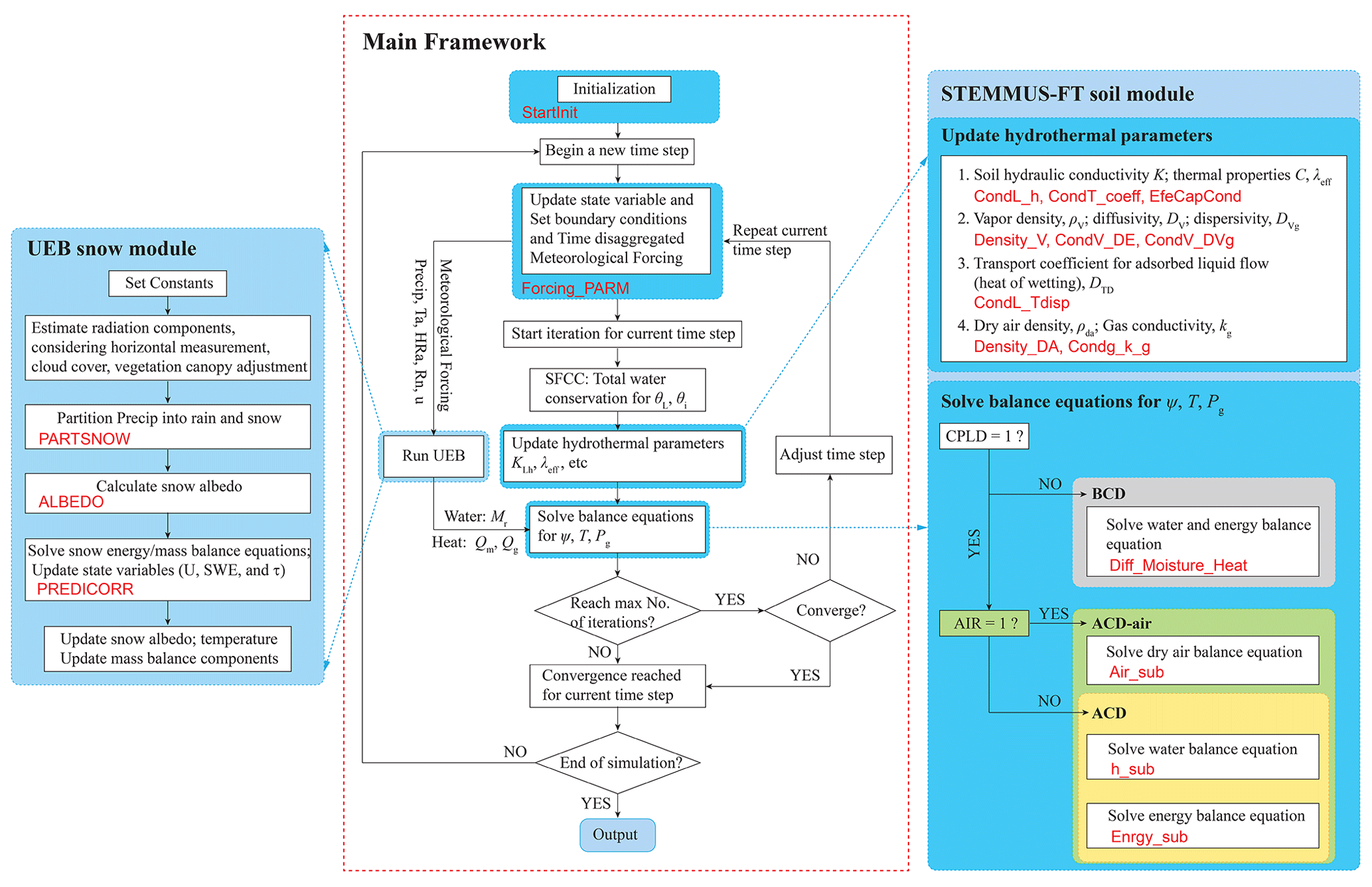
Figure 1The overview of the coupled STEMMUS-FT and UEB model framework and model structure. SFCC is soil freezing characteristic curve, θL and θi are soil liquid water and ice content, KLh is soil hydraulic conductivity, and λeff is thermal conductivity. are the state variables for soil module STEMMUS-FT (matric potential, temperature, and air pressure, respectively). U, SWE, and τ are the state variables for snow module UEB (snow energy content, snow water equivalent, and snow age, respectively). UEB is the Utah energy balance module. Precip, Ta, HRa, Rn, and u are the meteorological inputs (precipitation, air temperature, relative humidity, radiation, and wind speed, respectively). Mr is the snowmelt water flux, Qm is the convective heat flux due to snowmelt water, and Qg is the heat conduction flux. Model subroutines are in red.
Table 2Main subroutines in STEMMUS-UEB.
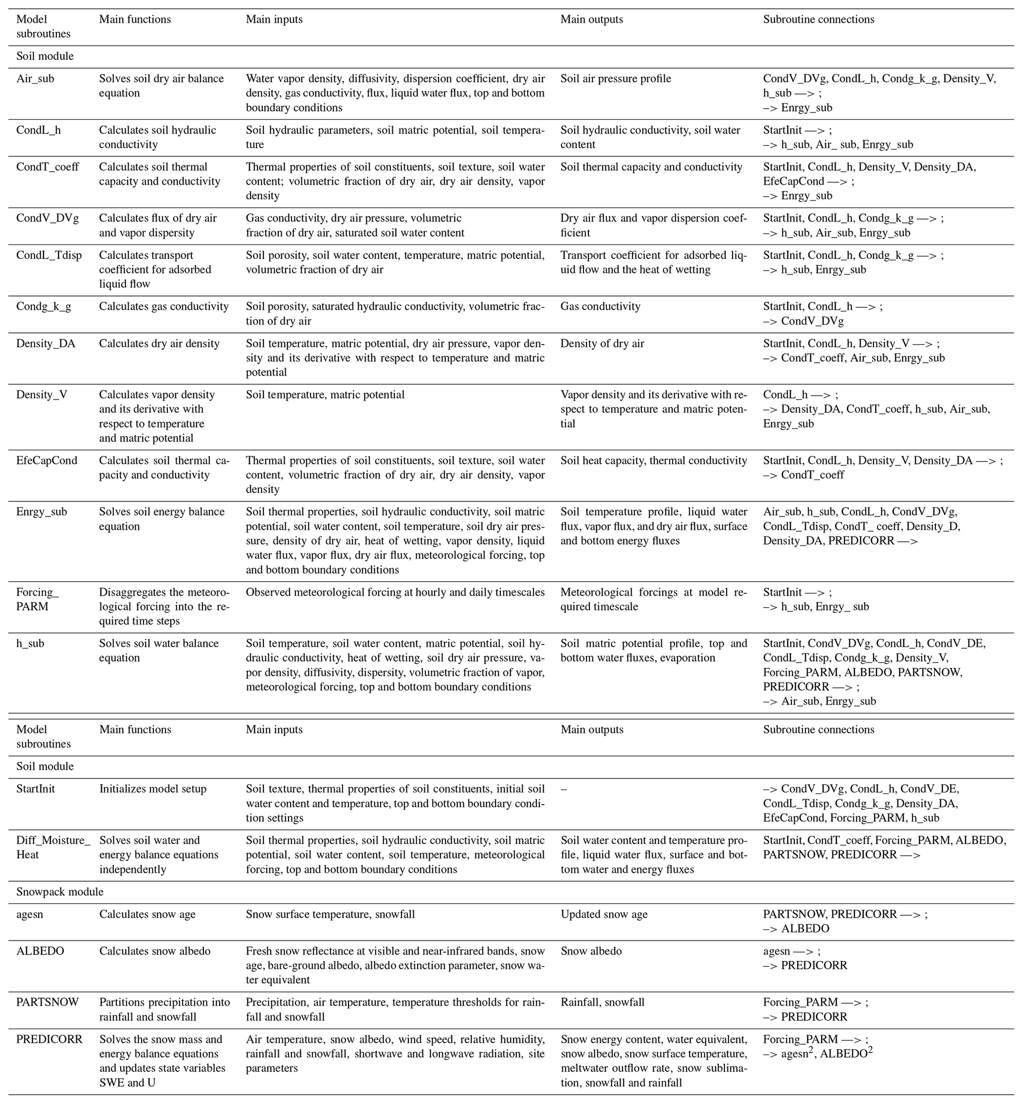
Note that —> means the relevant subroutines that are incoming to the current one, and –> means the relevant subroutines for which the current subroutine is output to. agesn2 and ALBEDO2 mean the use of subroutines agesn and ALBEDO after solving the snowpack energy and mass conservation equations to update the snow age and albedo, respectively.
2.2 Soil mass and heat transfer module
The detailed physically based two-phase flow soil model (STEMMUS) was first developed to investigate the underlying physics of soil water, vapor, and dry air transfer mechanisms and their interaction with the atmosphere (Zeng et al., 2011a, b; Zeng and Su, 2013). It is achieved by simultaneously solving the balance equations of soil mass, energy, and dry air in a fully coupled way. The mediation effect of vegetation on such interactions was recently incorporated via the root water uptake sub-module (Yu et al., 2016) and by coupling with the detailed soil and vegetation biogeochemical process (Wang et al., 2021; Yu et al., 2020a). It facilitates our understanding of the hydrothermal dynamics of respective components in the frozen soil medium (i.e., soil liquid water, water vapor, dry air, and ice) by implementing the freeze–thaw process (hereafter STEMMUS-FT, for applications in cold regions, Yu et al., 2018a, 2020c).
The frozen soil physics considered in STEMMUS-FT includes three parts: (i) the ice blocking effect on soil hydraulic conductivities (see Sect. S2.2.2 in the Supplement), (ii) the inclusion of ice effect in the calculation of soil thermal capacity and conductivity (see Sect. S2.2.8), and (iii) the exchange of latent heat flux during phase change periods. With the aid of Clausius–Clapeyron relation, which characterizes the phase transition between liquid and solid phase in the thermal equilibrium system, the soil water characteristic curve (e.g., van Genuchten, 1980) is then extended to consider the freezing temperature dependence, i.e., soil freezing characteristic curve (Hansson et al., 2004; Dall'Amico et al., 2011). The fraction of soil liquid–solid water at a given temperature was then calculated prognostically with the soil freezing characteristic curve. Soil hydraulic parameters were further used in the Mualem (1976) model to compute the soil hydraulic conductivity. The ice effect is considered by reducing the soil saturated hydraulic conductivity as a function of ice content (Yu et al., 2018a).
In response to minimize the potential model-comparison uncertainties from various model structures and to figure out which process matters, three levels of complexity of mass and heat transfer physics are made available in the current STEMMUS-FT modeling framework (Yu et al., 2020c). First, the 1D Richards equation and heat conduction were deployed in STEMMUS-FT to describe the isothermal water flow and heat flow (termed BCD). The BCD model considers the interaction of soil water and heat transfer implicitly via the parameterization of heat capacity, thermal conductivity, and the water phase change effect. The water flow is fully affected by soil temperature regimes in the advanced coupled water and heat transfer model (termed ACD model). The movement of water vapor, as the primary linkage between soil water and heat flow, is explicitly characterized. STEMMUS-FT further enables the simulation of temporal dynamics of three water phases (liquid, vapor, and ice), together with the soil dry air component (termed ACD-air model). The governing equations of liquid water flow, vapor flow, airflow, and heat flow were listed in Appendix A1 (see the more detailed model description in Zeng et al., 2011a, b; Zeng and Su, 2013; Yu et al., 2018a, 2020c).
2.3 Snowpack module UEB
The Utah energy balance snowpack model (UEB; Tarboton and Luce, 1996) is a single-layer physically based snow accumulation and melt model. Two precipitation types, i.e., rainfall and snowfall, are discriminated by their dependence on air temperature. The snowpack is characterized using two primary state variables, snow water equivalent (SWE), and the internal energy U. Snowpack temperature is expressed diagnostically as the function of SWE and U together with the states of the snowpack (i.e., solid, solid and liquid mixture, and liquid). Given the insulation effect of the snowpack, snow surface temperature differs from the snowpack bulk temperature, which is mathematically considered using the equilibrium method (i.e., balances energy fluxes at the snow surface). The age of the snow surface, as the auxiliary state variable, is utilized to calculate the snow albedo (see Appendix A3). When the snowpack is shallow, the albedo is the weighting function of the snow albedo and the bare-ground albedo. The solar radiation penetration in the shallow snowpack is exponentially attenuated and expressed in the weighting factor. The melt outflow is calculated using Darcy's law with the liquid fraction as inputs. The conservation of mass and energy forms the physical basis of UEB (Tarboton and Luce, 1996, as presented in Appendix A2).
UEB is recognized as one simple yet physically based snowmelt model. It captures the snow process well (e.g., diurnal variation of meltwater outflow rate, snow accumulation, and ablation; see the general overview of UEB model development and applications in Table S6.3). It requires little effort in parameter calibration and can be easily transferable and applicable to various locations (e.g., Gardiner et al., 1998; Schulz and de Jong, 2004; Watson et al., 2006; Sultana et al., 2014; Pimentel et al., 2015; Gichamo and Tarboton, 2019), especially for data-scarce regions like the Tibetan Plateau. We thus selected the original parsimonious UEB (Tarboton and Luce, 1996) as the snow module to be coupled with the soil module (STEMMUS-FT).
2.4 Configurations of numerical experiments
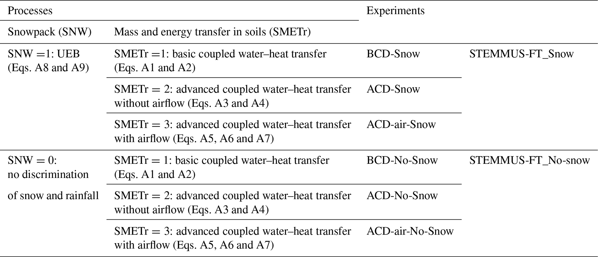
On the basis of the aforementioned STEMMUS-UEB coupling framework, the various complexities of vadose zone physics were further implemented as three alternative model versions. First, the soil ice effect on soil hydraulic and thermal properties and the heat flow due to the water phase change were taken into account, while the water and heat transfer is not coupled in STEMMUS-FT and is termed the BCD model. Second, the STEMMUS-FT with the fully coupled water and heat transfer physics (i.e., water vapor flow and thermal effect on water flow) was applied and termed the ACD model. Lastly, on top of the ACD model, the air pressure was independently considered as a state variable (therefore, the airflow) and termed the ACD-air model. With the abovementioned model versions (STEMMUS-FT_Snow), taking into account the no-snow scenarios (STEMMUS-FT_No-Snow), Table 3 lists the configurations of all six designed numerical experiments. The model parameters used for all simulations for the tested experimental site are listed in Table S6.2.
Table 3Numerical experiments with various mass and energy transfer schemes with and without explicit consideration of snow cover (Eqs. A1–A7 are listed in Appendix A1; Eqs. (A8)–(A9) are listed in Appendix A2).
2.5 Description of the tested experimental sites
Maqu station, equipped with a catchment-scale soil moisture and soil temperature (SMST) monitoring network and micro-meteorological observing system, is situated on the northeastern edge of the Tibetan Plateau (Su et al., 2011; Dente et al., 2012; Zeng et al., 2016). According to the updated Köppen–Geiger climate classification system, it can be characterized as a cold climate with dry winter and warm summer. The annual mean precipitation is about 620 mm, and the annual average potential evaporation is about 1353.4 mm. Precipitation in Maqu is uneven over the year, with most of the precipitation events occurring from May to October and little precipitation or snowfall during the wintertime. The average annual air temperature is 1.2 ∘C, and the mean air temperatures of the coldest month (January) and the warmest month (July) are about −10.0 and 11.7 ∘C, respectively. Alpine meadows (e.g., Cyperaceae and Gramineae), with a height varying from 5 to 15 cm throughout the growing season, are the dominant land cover in this region. This site is seasonally snow covered, with temporal snow in the non-growing season, which is due to the intermittent snowfall and the rapid snow melting and sublimation caused by the high air temperature and strong solar radiation in the daytime. The general soil types are sandy loam, silt loam, and organic soil for the upper soil layers (Dente et al., 2012; Zheng et al., 2015; Zhao et al., 2018a). The soil texture and hydraulic properties were listed in Table S6.2, and how these were used in STEMMUS-UEB is illustrated in Fig. 1 and Table 2.
The Maqu SMST monitoring network spans an area of approximately 40 km × 80 km with an elevation ranging from 3200 m to 4200 m a.s.l. (– N, – E). SMST profiles are automatically measured by 5TM ECH2O probes (METER Group, Inc., USA) installed at different soil depths, i.e., 5, 10, 20, 40, and 80 cm. The micro-meteorological observing system consists of a 20 m planetary boundary layer (PBL) tower providing the meteorological measurements at five heights above ground (i.e., wind speed and direction, air temperature and relative humidity), and an eddy covariance system (EC150, Campbell Scientific, Inc., USA) equipped for measuring the turbulent sensible and latent heat fluxes and carbon fluxes. The equipment for four-component downwelling and upwelling solar and thermal radiation (NR01-L, Campbell Scientific, Inc., USA) and liquid precipitation (T200B, Geonor, Inc., USA) are also deployed. A dataset from 1 December 2015 to 15 March 2016 was utilized in this study. Independent precipitation data (3 h time interval) during the same testing period from an adjacent meteorological station were used as the mutual validation data.
Yakou super snow station ( N, E, 4145 m) is located in the upstream Heihe basin in the northeastern Tibetan Plateau. It is a high-elevation snow-covered site with the wet summers and dry winters. The dominant land type is tundra with frozen ground below. There is a unique seasonal variation of snow depth with the maximum snow depth usually being in the springtime (32 cm during the period 2014–2017). Loam is the main soil type with the silt loam near the surface and sandy soil for the deeper soil layers.
The integrated hydrometeorological, snow cover, and frozen ground data were published and available from the Cold and Arid Regions Science Data Center at Lanzhou (Che et al., 2019; Li et al., 2019; Li, 2019). The meteorological data (air temperature, wind speed, precipitation, downward shortwave and longwave radiation, and relative humidity) were recorded by the automatic meteorological station (AMS). In situ measurements of snow cover properties (snow depth and snow water equivalent) were obtained using the state-of-the-art instruments (SR50A and GammaMONitor, Campbell Scientific, USA). Soil moisture profiled at 4, 10, 20, 40, 80, 120, and 160 cm soil depth was measured using ECH2O-5 probes (METER Group, Inc., USA). In addition to the seven soil depths, the surface soil temperature (0 cm) was also recorded using the Avalon AV-10T sensors (Avalon Scientific, Inc., USA). The eddy covariance system was equipped at the Yakou site for measuring land surface turbulent fluxes. The dataset from 1 September to 31 December 2016 was used to validate the model performance in mimicking the dynamics of snow water equivalent, soil hydrothermal regimes, and land surface evaporation. The calibrated soil hydraulic and snow cover properties were listed in the Supplement in Table S6.2.
3.1 Albedo
The time series of surface albedo, calculated as the ratio of upwelling shortwave radiation to the downwelling shortwave radiation and estimated using BCD, ACD, and ACD-air models, is shown in Fig. 2 together with precipitation. As the snowpack has a higher albedo than the underlying surface (e.g., soil, vegetation) compared to the observations, models without snow module presented a relatively flat variation of daily average surface albedo and lacked the response to the winter precipitation events (Fig. 2, Table 4). With the snow module, STEMMUS-UEB models can mostly capture the abrupt increase of surface albedo after winter precipitation events. The mismatches in terms of the magnitude or absence of increased albedo after precipitation events indicated that the model tended to underestimate the albedo dynamics. The shallow snowfall events might be not well captured by the model (see Sect. 4.1). Three model versions (BCD-Snow, ACD-Snow, and ACD-air-Snow) produced similar fluctuations regarding the presence of snow cover with slight differences in terms of the magnitude of albedo.
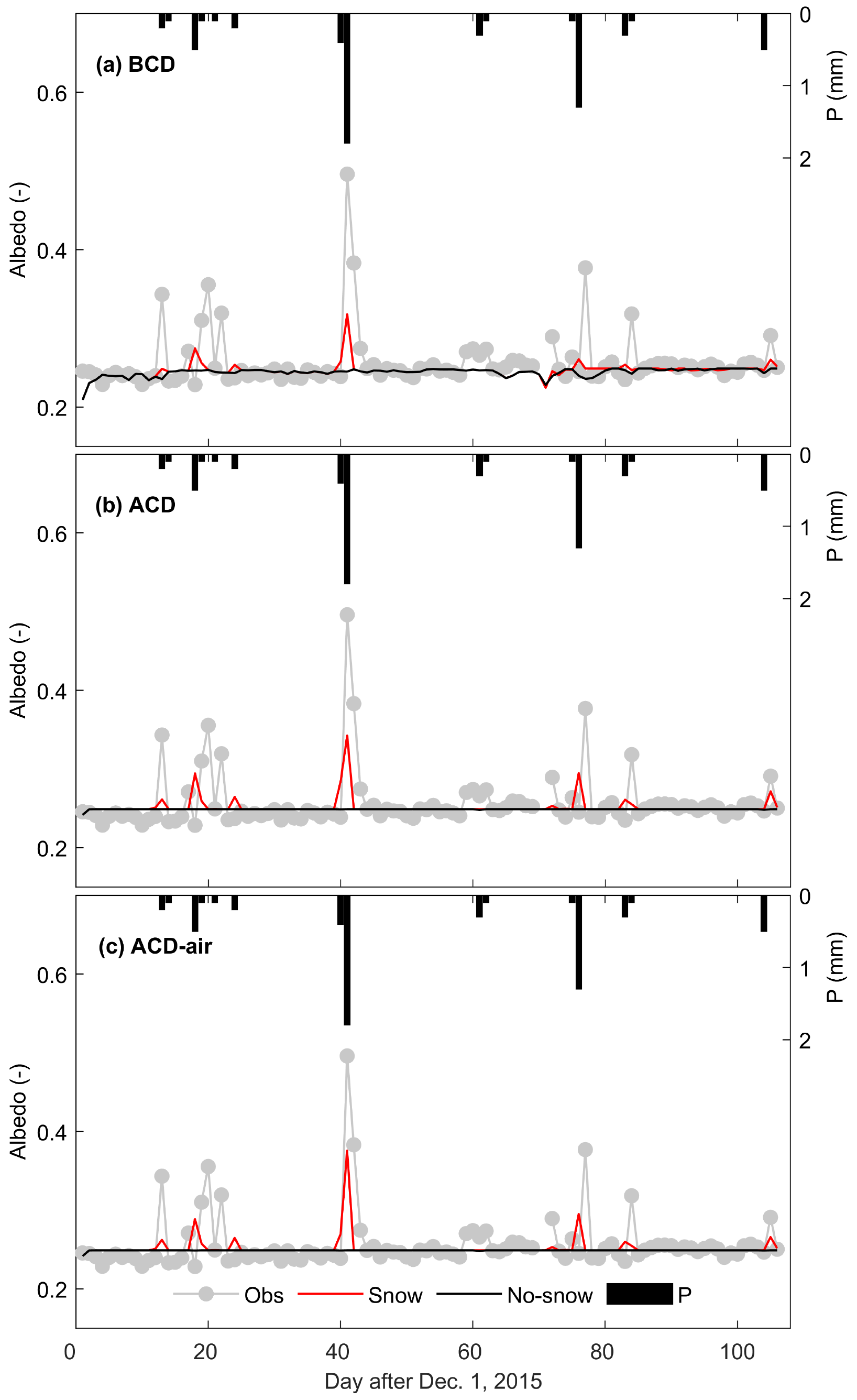
Figure 2Time series of observed and model simulated daily average albedo using (a) BCD, (b) ACD, and (c) ACD-air soil models with and without consideration of the snow module (including precipitation).
Table 4Comparative statistics values of various model versions for snow albedo, LE, soil temperature, and soil moisture. The best statistical performance is highlighted in bold font, while the values with poor statistical model performance are highlighted in italic font.

Note that BIAS , , and RMSE , where yi and are the measured and model simulated values of the selected variable (snow albedo, latent heat flux or LE, and soil temperature and moisture), is the mean value of the measurements of the selected variable (snow albedo, LE, and soil temperature and moisture), and n is the number of data points. The correlations are all significant at the 0.01 level excluding values marked with “–”, which indicates that the correlation is not significant.
3.2 Soil temperature and moisture dynamics
The observed spatial and temporal dynamics of soil temperature from five soil layers were used to verify the performance of different models (Fig. 3). The initial soil temperature state can be characterized as the warm bottom and cool surface soil layers (based on in situ observations). The freezing front (indicated by the zero-degree isothermal line, ZDIL) developed downwards rapidly until the 70th day after 1 December 2015, when it reached its maximum depth. Following this, the freezing front stabilized as an offset effect of latent heat release (termed the zero-curtain effect). Such influence can be sustained until all the available water to that layer is frozen, at which point the latent heat effect is negligible compared to the heat conduction. At shallower layers, the atmospheric forcing dominates the fluctuation of thermal states. The isothermal lines (e.g., −2 ∘C) had a larger variation than that of ZDIL. At deeper soil layers, the temporal dynamics of isothermal lines were smoother than that of ZDIL, indicating that the effect of fluctuated atmospheric force on soil temperature was damped with the increase of soil depth. Compared to the observations, BCD-Snow model presented an earlier development of the freezing front and arrival of the maximum freezing depth (60th day after 1 December 2015). The deeper and more fluctuated freezing front indicates that a stronger control of atmospheric forcing on soil thermal states was produced by BCD-Snow model. The ACD models can capture the propagation characteristic of the freezing front well in terms of the variation magnitude and maximum freezing depth. There is no significant difference in soil thermal dynamics between the model with and without the snow module, except at the surface soil layers (Table 4).
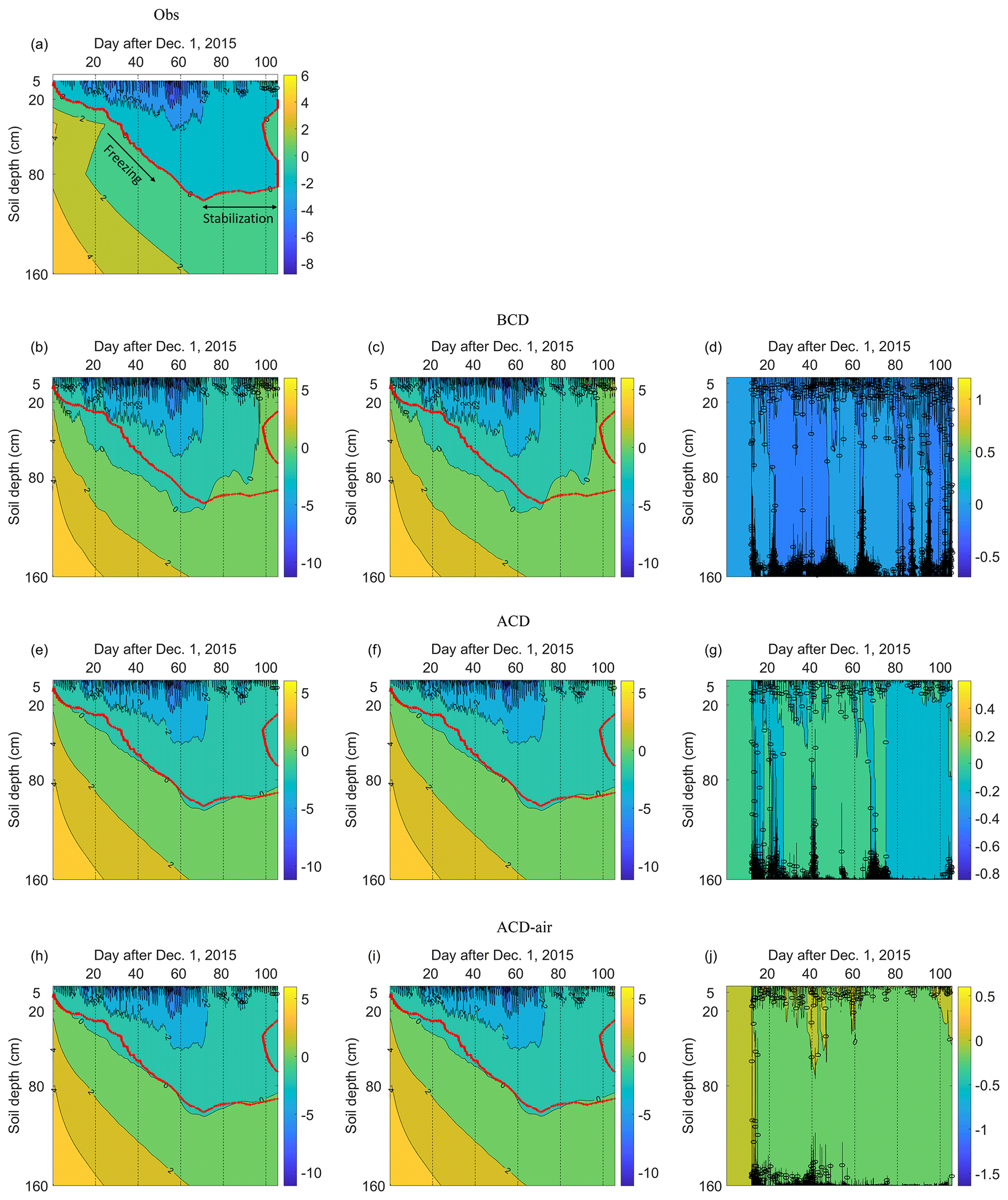
Figure 3The spatial and temporal dynamics of observed (a) and simulated soil temperature using BCD, ACD, and ACD-air soil models both with and without consideration of the snow module (snow: b, e, h; no snow: c, f, i) and the difference between them (d, g, j) (simulations with snow minus simulations without snow). The red line indicates the zero-degree isothermal line (ZDIL) from the measured soil temperature. The observed soil freezing stage and stabilization stage is marked in Fig. 3a.
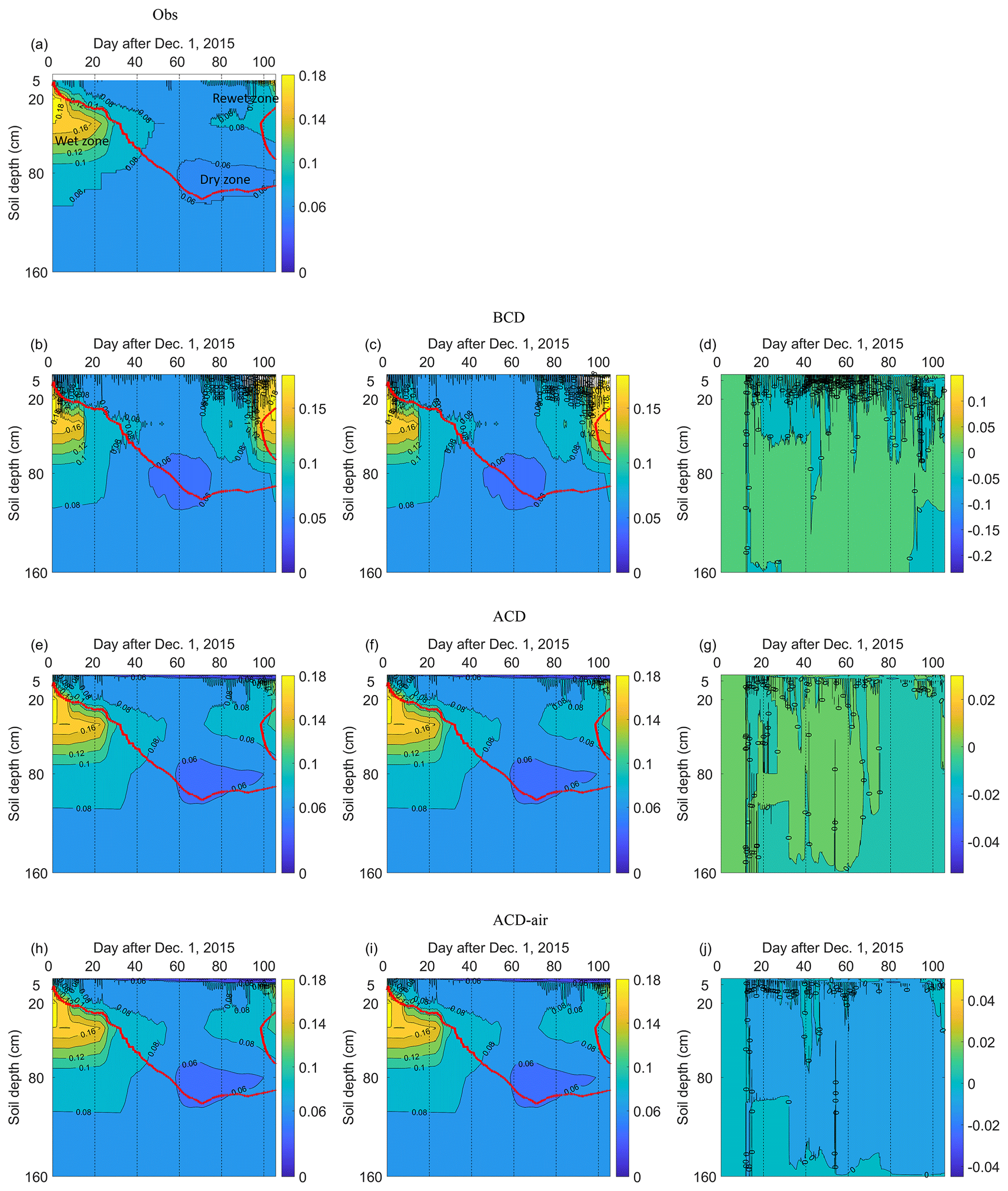
Figure 4The spatial and temporal dynamics of observed (a) and simulated soil volumetric water content using BCD, ACD, and ACD-air soil models both with and without consideration of the snow module (snow: b, e, h; no snow: c, f, i) and the difference between them (d, g, j) (simulations with snow minus simulations without snow). The red line indicates the ZDIL from the measured soil temperature. The observed wet zone, dry zone, and rewet zone of soil moisture is indicated in Fig. 4a.
Figure 4 shows the spatial and temporal dynamics of observed and simulated soil water content in the liquid phase (SWCL). The SWCL of active layers depends to a large extent on the soil freezing and thawing status. Soil is relatively wet at soil layers of 10–60 cm for the starting period. Its temporal development was disrupted by the presence of soil ice and tended to increase wetness during the thawing period. A relatively dry zone (θL<0.06 m3 m−3) above the freezing front was found, indicating the nearly completely frozen soil during the stabilization stage. The initial wet zone of soil moisture was narrowed down and the rewetting zone tended to enlarge from BCD-Snow simulation due to its early freezing and thawing of soil (Fig. 4b). The position of the dry zone occurred earlier due to the early reaching of the stabilization period in the BCD-Snow model (Fig. 3b). For the ACD models, the position and development of initial wet zone, rewetting zone, and dry zone are similar to those from the observations, indicating the soil moisture dynamics can be captured well by the ACD models. Compared to the STEMMUS-FT_Snow model, there was no observable difference in the SWCL dynamics at deeper soil layers from STEMMUS-FT_No-Snow simulations. The surface SWCL was found affected from STEMMUS-FT_Snow simulations (Table 4).
3.3 Surface latent heat flux
Figure 5 shows the comparison of time series of observed and model-simulated surface cumulative latent heat flux using three models with and without consideration of the snow module. Considerable overestimation of latent heat flux was produced by the BCD-Snow model: 121.79 % more than was observed. Such overestimations were largely reduced by ACD and ACD-air models. There is a slight underestimation of cumulative latent heat flux in the ACD-Snow and ACD-air-Snow models, with values of −8.33 % and −7.05 %, respectively. Compared with STEMMUS-FT_Snow simulations, there is less latent heat flux produced by the STEMMUS-FT_No-snow simulations. This is mainly due to the sublimation of snow cover, which cannot be simulated by the STEMMUS-FT_No-snow models. The difference in cumulative latent heat flux between STEMMUS-FT with and without snow module increases from BCD to ACD-air schemes, with the values of 2.02 %, 7.69 %, and 8.97 % for BCD, ACD, and ACD-air schemes, respectively.
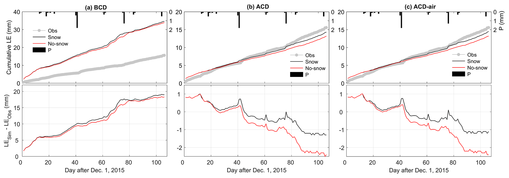
Figure 5Time series of observed and model simulated surface cumulative latent heat flux (LE) using (a) BCD, (b) ACD, and (c) ACD-air soil models with and without consideration of the snow module (including precipitation). The top row shows the comparisons, and the bottom row shows the model bias of the cumulative surface LE.
3.4 Liquid and vapor fluxes
To further elaborate the effect of snowpack on LE, we presented the diurnal variations of LE and its components at two typical episodes with precipitation events (freezing and thawing period, respectively). The relative contribution of liquid and vapor flow to the total mass transfer after precipitation events was separately presented in Figs. 8 and 9, i.e., the liquid water flux driven by temperature qLT, matric potential qLh and air pressure qLa, water vapor flux driven by temperature qVT, matric potential qVh, and air pressure qVa.
3.4.1 LE
Diurnal dynamics of the observed and simulated latent heat flux during the rapid freezing period with the occurrence of precipitation events, from 10th to 14th days after 1 December 2015, are shown as Fig. 6a, b, and c. Compared to the observations, the diurnal variations of latent heat flux were captured by the proposed model with various levels of complexities. Performance of BCD, ACD, and ACD-air models in simulating LE differed mainly regarding the magnitude and response to precipitation events. For the BCD-Snow model, the overestimation of LE was found at the 10th and 11th day after 1 December due to relatively high surface soil moisture simulation (Fig. S6.1b). A certain amount of enhanced surface evaporation was produced shortly after precipitation, which is most probably due to the snow sublimation. Snow sublimation does not appear to intuitively match with observations. The mismatch in the LE enhancement after precipitation events can be attributed to the fact that the partition process of precipitation into various components (rainfall, snowfall, canopy interception) might not be captured by the model well. Such a response to the winter precipitation events was absent from the BCD-No-Snow simulations.
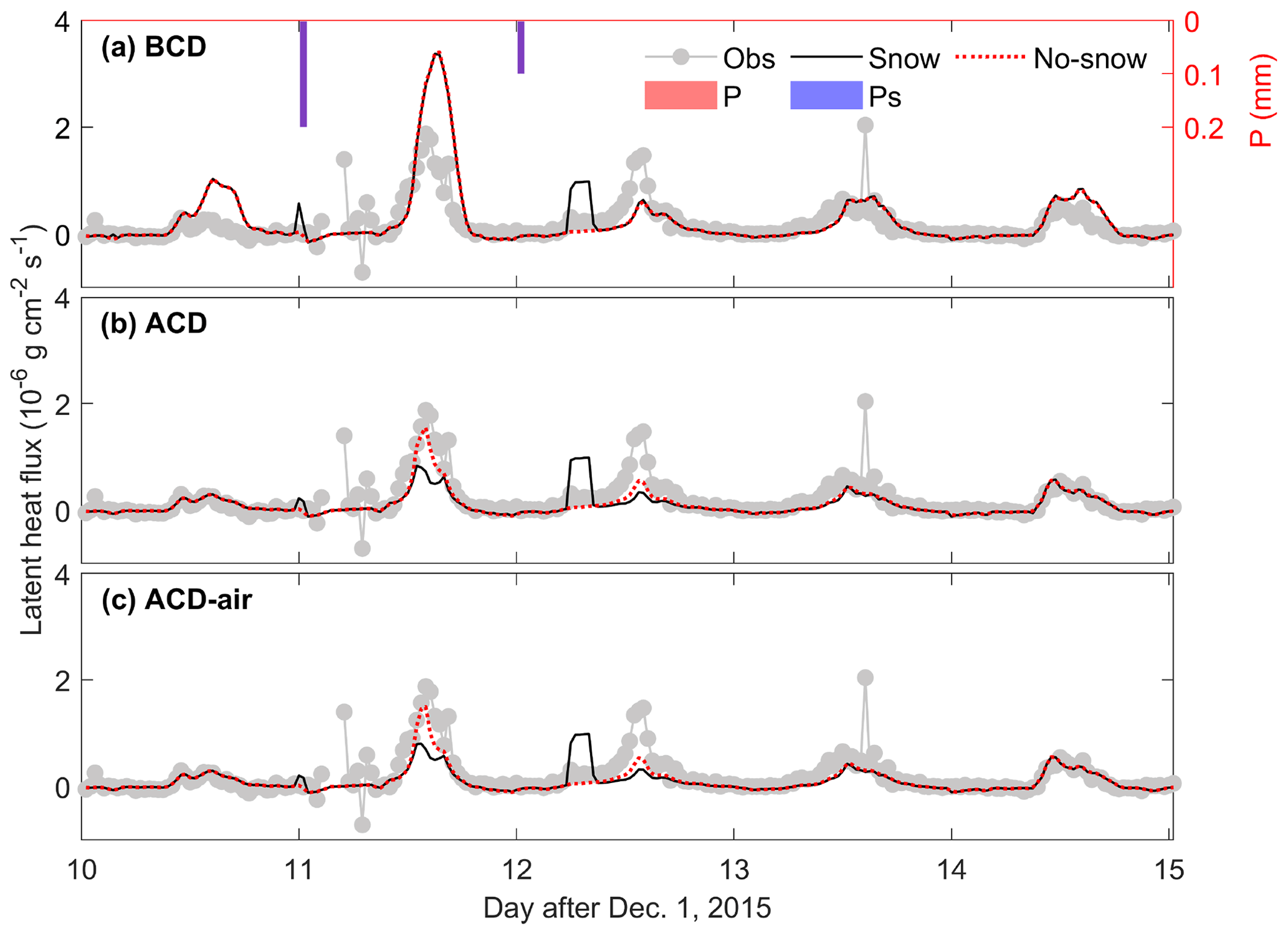
Figure 6Observed and model simulated latent heat flux using (a) BCD, (b) ACD, and (c) ACD-air soil models with and without the snow module of a typical 5 d freezing period (from the 10th to 14th day after 1 December 2015). P is the precipitation and Ps is the snowfall. All precipitation is in the form of snowfall.
The overestimation of LE was reduced by ACD and ACD-air models (Fig. 6b and c). Compared to the ACD-Snow model simulations, the ACD-No-snow model produced a stronger diurnal variation of LE after the precipitation and is approaching the measured LE. Lower diurnal variation of LE for the ACD-Snow model can be ascribed to the lower surface SWCL (see Fig. S6.1d and g). For the ACD-Snow model, precipitation was partitioned into rainfall and snowfall, part of which was directly evaporated as sublimation. The sum of rainfall and the melting part of snowfall reached the soil surface as the incoming water flux, which is less than that for the ACD-No-snow model (taking all the precipitation as the incoming water flux). There is no significant difference in the dynamics of LE between simulations by ACD models and ACD-air models.
During the thawing period, the diurnal variations of LE were simulated well by the models (Fig. 7). There are some discrepancies regarding the peak values of LE. For the BCD-Snow model, overestimations were found in 100th, 101st, and 102nd day after 1 December 2015. The high LE values on 100th and 101st day are probably due to the high surface soil moisture by the thawing water (Fig. S6.2b), whereas on the 102nd day it is due to the snow sublimation (Fig. 7a). The peak values were reproduced but shifted by BCD-No-Snow simulation, which occurred on 100th day and at the end of 102nd day, indicating the shift of surface soil moisture states (Fig. S6.2b).
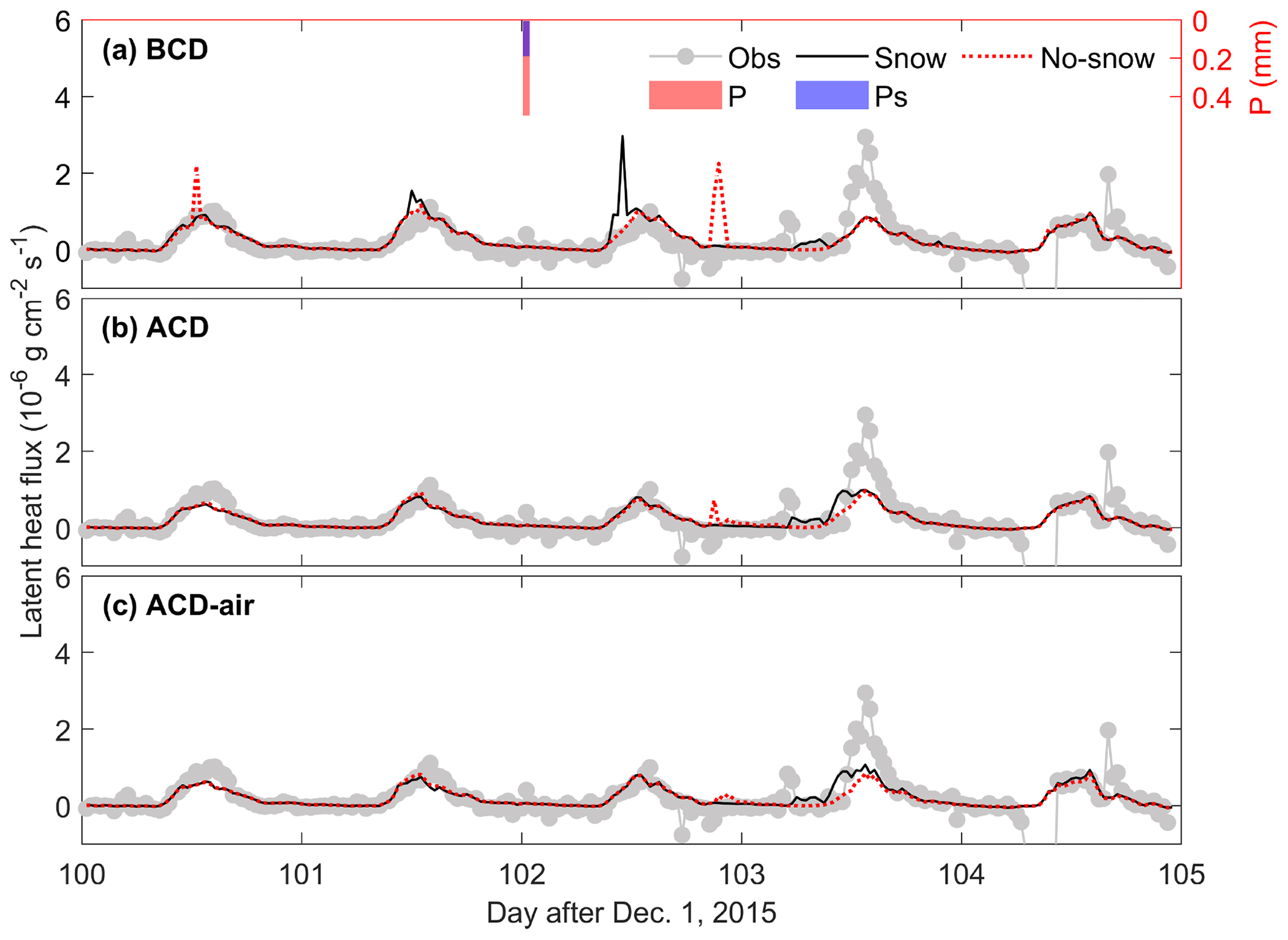
Figure 7Observed and model simulated latent heat flux using (a) BCD, (b) ACD, and (c) ACD-air soil models with and without the snow module of a typical 5 d thawing period (from the 100th to 104th day after 1 December 2015). P is the precipitation and Ps is the snowfall.
For the ACD model, the difference in latent heat flux between snow and no-snow simulations was noticeable 2 d after precipitation. The larger values of LE from the ACD-No-snow model occurred earlier than those from the ACD-Snow model due to the earlier response of surface soil moisture to the precipitation event (Fig. S6.2). Compared to the observations, the enhancement of LE advanced from the ACD-Snow simulations (Fig. 7b). This enhanced evaporation can be attributed to the snow sublimation and increased surface soil moisture content. Similar lag behavior of precipitation-enhanced evaporation was produced by the ACD-air-Snow models (Fig. 7c). There are mismatches in the time and magnitude of LE enhancement between ACD-Snow model simulations and observations (Fig. 7b). This discrepancy lies in the uncertainties of snowpack simulations, which can be attributed to either the inaccurate precipitation measurements (Barrere et al., 2017; Günther et al., 2019) or to the fact that the precipitation partition process is not described well by the model (Harder and Pomeroy, 2014; Ding et al., 2017).
3.4.2 LE and decomposition of surface mass transfer
During the freezing period, the soil water vapor rather than the liquid water flux dominated the surface mass transfer process. Missing the description of the vapor diffusion process hindered the BCD models ability to realistically depict the decomposition of surface mass transfer dynamics (Fig. 8a and b).
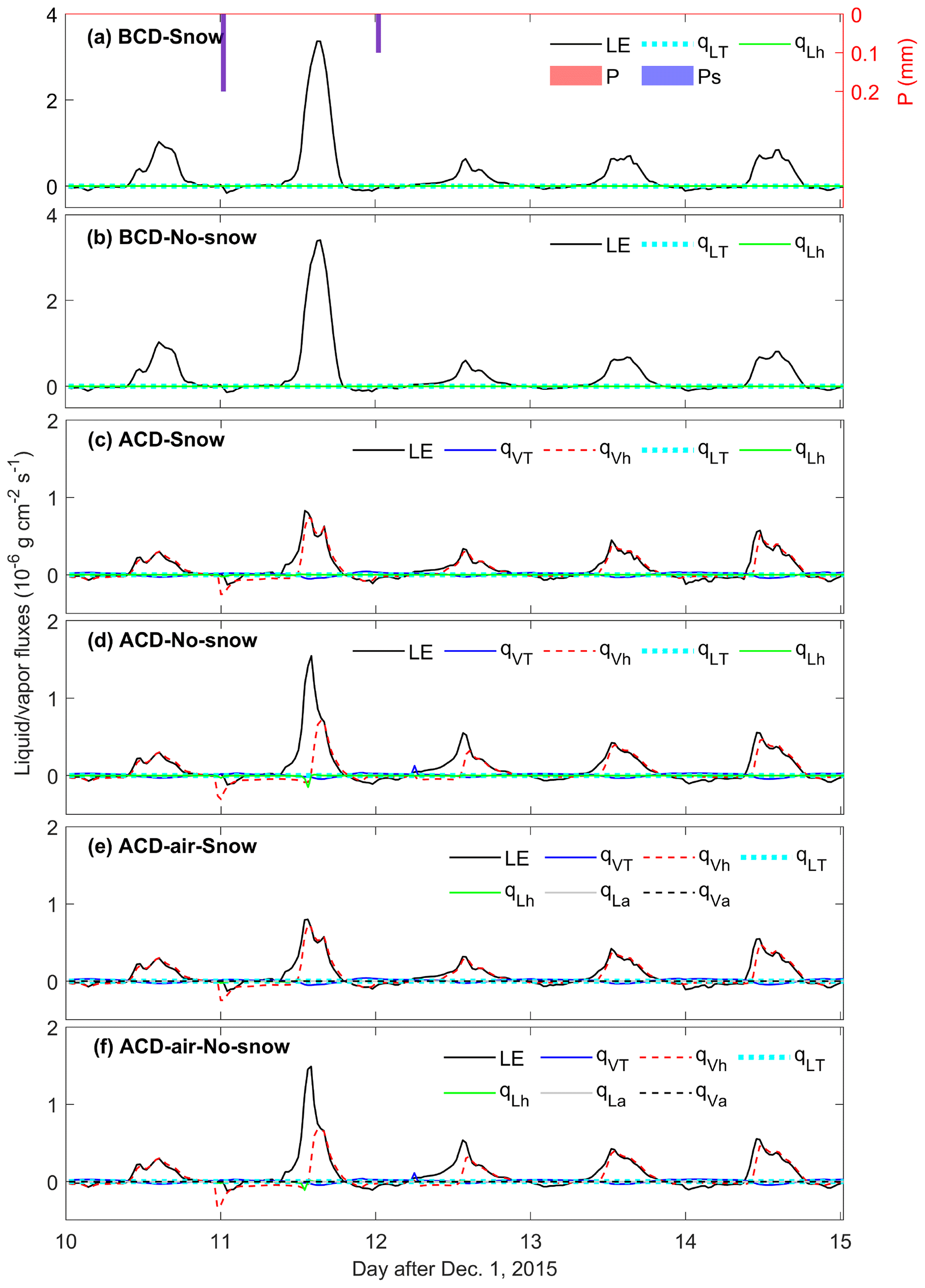
Figure 8Model-simulated latent heat flux and surface soil (0.1 cm) thermal and isothermal liquid water and vapor fluxes (LE, qVT, qVh, qLT, qLh, qLa, qVa) with and without the snow module of a typical 5 d freezing period (from the 10th to 14th day after 1 December 2015). Panels (a), (c), and (e) are the surface soil thermal and isothermal liquid water and vapor fluxes simulated by the BCD-Snow, ACD-Snow, and ACD-air-Snow models, respectively. Panels (b), (d), and (f) are the surface soil thermal and isothermal liquid water and vapor fluxes simulated by the BCD-No-Snow, ACD-No-Snow, and ACD-air-No-Snow models, respectively. LE is the latent heat flux, qVT and qVh are the water vapor fluxes driven by temperature and matric potential gradients, respectively, qLT and qLh are the liquid water fluxes driven by temperature and matric potential gradients, respectively, and qLa and qVa are the liquid and vapor water fluxes driven by air pressure gradients, respectively. Positive and negative values indicate upward and downward fluxes, respectively. Note that the surface LE fluxes without snow sublimation are presented here. P is the precipitation, and Ps is the snowfall. All precipitation is in the form of snowfall.
There is a visible diurnal variation of thermal vapor flux qVT from the ACD model simulation (Fig. 8c and d). The isothermal vapor flux qVh contributed to most of the mass transfer during the freezing period. It should be noted that the sum of water–vapor fluxes at the 0.1 cm soil layer cannot balance the surface evaporation, especially after the precipitation events (Fig. 8c). We assumed this premise and attributed it to the surface ice sublimation process. Precipitation water was frozen on the soil surface, and only vapor fluxes are active in the topsoil layers. Sublimation of surface ice may contribute to the gaps between liquid–vapor fluxes and LE (Yu et al., 2018a). As more precipitation water was frozen on the soil surface from the ACD-No-Snow model (Fig. 8d), the difference between the sum of water–vapor fluxes at the top 0.1 cm soil layer and the surface evaporative water enlarged compared to ACD-Snow simulations. Thermal liquid water flux qLT appears negligible to the total mass flux during the whole simulation period. There is no significant difference recognized in the mass transfer between the ACD-air and ACD during the freezing period.
During the thawing period, a certain amount of upward liquid water flux was produced by the BCD model, supplying the water to the topsoil and evaporate into the atmosphere (Fig. 9a and b). Compared to the isothermal liquid flux qLh, the thermal liquid flux qLT was negligible to the total mass flux.
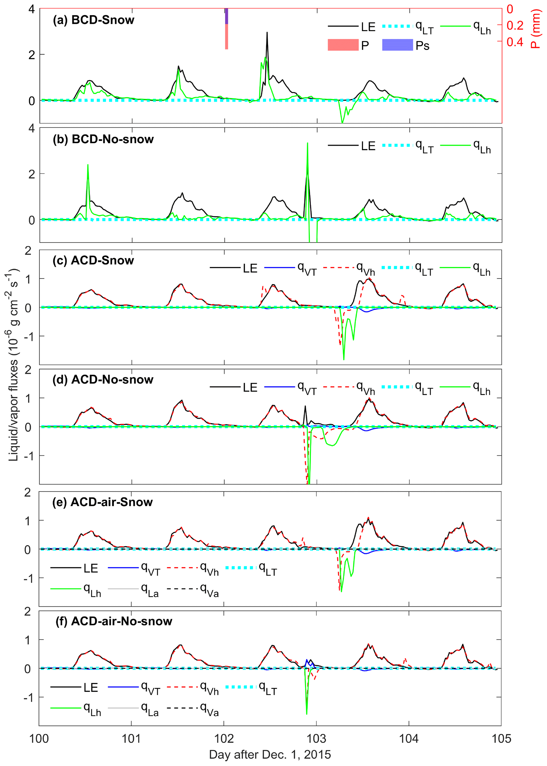
Figure 9Model-simulated latent heat flux and surface soil (0.1 cm) thermal and isothermal liquid water and vapor fluxes (LE, qVT, qVh, qLT, qLh, qLa, qVa) using BCD (a, b), ACD (c, d), and ACD-air (e, f) simulations with and without the snow module, respectively, during the typical 5 d thawing periods (from the 100th to 104th day after 1 December 2015). Panel (a), (c), and (e) are the surface soil thermal and isothermal liquid water and vapor fluxes simulated by BCD-Snow, ACD-Snow, and ACD-air-Snow model, respectively. Panels (b), (d), and (f) are the surface soil thermal and isothermal liquid water and vapor fluxes simulated by BCD-No-Snow, ACD-No-Snow, and ACD-air-No-Snow model, respectively. LE is the latent heat flux, qVT and qVh are the water vapor fluxes driven by temperature and matric potential gradients, respectively, qLT and qLh are the liquid water fluxes driven by temperature and matric potential gradients, respectively, and qLa and qVa are the liquid and vapor water fluxes driven by air pressure gradients, respectively. Positive and negative values indicate upward and downward fluxes, respectively. Note that the surface LE fluxes without snow sublimation are presented here. P is the precipitation, and Ps is the snowfall.
For the ACD model, the diurnal variation of thermal vapor flux qVT was enhanced after precipitation, producing a larger amount of upward and downward vapor flux during the nighttime and daytime, respectively (e.g., Fig. 9c). As the surface soil is relatively dry, the isothermal vapor flux qVh contributes nearly all of the mass flux during the selected thawing period. Driven by the matric potential gradient, a large amount of isothermal water vapor flux qVh, accompanied by downward liquid water flux qLh, can be found after the nighttime precipitation event (Fig. 9c, d, e, f). These precipitation-induced isothermal liquid–vapor fluxes were lagged and less intense from the ACD-Snow model than that from the ACD-No-Snow model simulation (e.g., Fig. 9c vs. Fig. 9d). The snowpack reduces the instant precipitation infiltration process and enables the snowmelt afterwards, which led to the lagged and weaker response of surface SWCL to the precipitation (Fig. S6.2). This breaks the balance between isothermal vapor flux and evaporative LE (around the 103rd day after 1 December 2015). Compared to the ACD-No-Snow model, the imbalance was enlarged for the ACD-Snow model during the thawing period (Fig. 9c and d).
Compared to the ACD-No-Snow simulations, the upward thermal vapor flux qVT was enhanced after precipitation for the ACD-air-No-Snow model (Fig. 9f). This enhanced upward vapor flux reduced the soil liquid water content at 0.1 cm (Fig. S6.2f) and decreased the soil hydraulic conductivity and then the downward isothermal liquid–vapor flux (qLh, qVh). Other than that there is no significant difference between the ACD-air model and the ACD model during the thawing period.
4.1 Uncertainties in simulations of surface albedo and limitations
After a winter precipitation event, land surface albedo increases considerably (Fig. 2), indicating the presence of the snowpack. However, such snowfall events were episodic with small magnitudes (similar to those in Li et al., 2017), which means that they are difficult to capture well. Such difficulties can be partially attributed to the inherent uncertainties in precipitation measurements (both the precipitation amount and types). Due to the spatial variability of precipitation, the accurate observation of winter precipitation has proven to be a challenge, especially during windy winters (Barrere et al., 2017; Pan et al., 2017). It is necessary to have more snowpack-relevant measurements (e.g., the high-resolution measurements of the spatiotemporal field of wind speed, precipitation, and snowpack variations) to understand the dynamics of snowpack and its effect on energy and water fluxes. Furthermore, the temporal resolution of precipitation measurements adopted in this study is relatively coarse (3 h). In the current precipitation partition parameterization, the amount of snowfall was determined as a function of precipitation and air temperature thresholds. Given the coarse temporal resolution of precipitation measurements, the model may produce a time shift of snowfall events or even the misidentification of snowfall. The simple relation between the air temperature and precipitation types may be not suitable for this region because air temperature is not the best indicator of precipitation types, as argued by Ding et al. (2014). Other factors, i.e., relative humidity, surface elevation, and wet-bulb temperature, are also very relevant and should be taken into account for the discrimination of precipitation types. The other uncertainty lies in the representation of the snow process. For example, the wind blow effect and canopy snow interception, which have been recognized as important to the accurate simulation of snowpack dynamics (Mahat and Tarboton, 2014), are not taken into account in detail. Last but not least, the interpretation of surface albedo dynamics needs to be adapted to the specific site, especially regarding the shallow snow situations (Ueno et al., 2007, 2012; Ding et al., 2017; Wang et al., 2017). The albedo of the underlying surface should also be properly accommodated to this Tibetan meadow system. Regardless of the aforementioned uncertainties, our proposed model was capable of capturing the surface albedo variations with precipitation (Fig. 2) and can be seen as acceptable for analyzing snow cover effects in such a harsh environment.
4.2 Snow-cover-induced evaporation enhancement
In contrast to precipitation water from rainfall, precipitation water from snowfall enters the soil considerably lagged in time due to the water storage by snow cover (You et al., 2019). With the snow module, precipitation was partitioned into rainfall and snowfall. Part of the snowfall evaporated into the atmosphere as sublimation, and the other part, together with the rainfall, infiltrated into the underlying soil. It resulted in the delay of incoming water to the soil with a lower amount compared to that without consideration of the snow module. This amount of incoming water increased the evaporation after precipitation (Figs. 6 and 7). The other source for the enhanced evaporation flux after precipitation is snow sublimation, which is absent from the model without the snow module. Sublimation occurs readily under certain weather conditions (e.g., with freezing temperatures, enough energy). It can be more active in regions with low relative humidity, low air pressure, and dry winds. Such an amount of sublimation has been reported as being important from the perspective of climate and hydrology (e.g., Strasser et al., 2008; Jambon-Puillet et al., 2018), especially in high-altitude regions with low air pressure. During the freezing period, the evaporation enhancement can be also sourced from the sublimation of surface ice. The amount of the ice sublimation appeared to decrease during the freezing period in the presence of a transient snowpack (e.g., Fig. 8c vs. Fig. 8d). This is consistent with the results of Hagedorn et al. (2007), who investigated the effect of snow cover on the mass balance of ground ice with an artificially continuous annual snow cover. According to their results, the snow cover enhanced the vapor transfer into the soil and thus reduced the long-term ice sublimation. The relative contribution of increased surface soil moisture, snow sublimation, and surface ice sublimation to the enhanced evaporation is dependent on the pre-precipitation soil moisture and temperature states, air temperature, and the time and magnitude of precipitation events. Under the conditions of the low pre-precipitation SWCL with a freezing soil temperature (e.g., Fig. 8e, 11th vs. 12th day after 1 December), the precipitation falls on the surface as snowfall and rainfall (most freezes as ice). The sublimation from surface ice can contribute to most of the total mass transfer (e.g., Fig. 8e, 11th day after 1 December). If the soil temperature rises above the freezing temperature, there will be no sublimation of surface ice, in terms of contributing to the enhanced evaporation (e.g., Fig. 9e, 102nd day after 1 December).
4.3 Snow cover impacts with different soil model complexities
The model with different complexities of soil mass and energy transfer physics behaves differently in response to the winter precipitation events. During the freezing period, there is no significant difference in soil moisture simulated using the BCD models with and without the snow module. The precipitation water freezes at the soil surface, which cannot be transferred downwards with the BCD model physics. The sublimation, from either the snow or the surface ice, contributes to the precipitation-enhanced evaporation for the BCD model. As with vapor flow, the surface ice increases the soil moisture at lower layers via the downward isothermal vapor flux (Fig. 8). The surface ice sublimation and increased moisture-induced soil evaporation enhancement can be identified from the ACD model simulation. The role of airflow was negligible for the mass transfer during the freezing period.
When it comes to the thawing period, the BCD model produced a certain amount of liquid water flow, contributing considerably to the mass transfer. The obvious fluctuation of SWCL was noticed due to the thawing water and precipitation event. The main source for the increased evaporation was interpreted as isothermal liquid water flow, while for the ACD model the situation becomes more complex. Thawing surface ice and snowmelt water may coexist at the soil surface, resulting in different soil moisture response to precipitation events. The ice sublimation, snow sublimation, and increased soil moisture contribute to the evaporation enhancement after precipitation. When considering airflow, dry air interacts with soil ice and liquid and vapor water in soil pores (Yu et al., 2018a) and alters the soil moisture state. It thus considerably changes the relative contribution of each component to the mass transfer (Fig. 9).
With the aim to investigate the hydrothermal effect of the snowpack on the underlying soil system, we developed the integrated process-based soil–snow–atmosphere model, STEMMUS-UEB v1.0.0, which is based on the easily transferable and physically based description of the snowpack process and the detailed interpretation of the soil physical process with various complexities. From STEMMUS-UEB simulations, snowpack affects not only the soil surface conditions (surface ice and SWCL) and energy-related states (albedo, latent heat flux) but also the transfer patterns of subsurface soil liquid and vapor flow. STEMMUS-FT model can mostly capture the abrupt increase of surface albedo after winter precipitation events with consideration of the snow module. There is a significant overestimation of cumulative surface latent heat flux by the BCD model. The ACD and ACD-air models produce a slight underestimation of cumulative LE compared to the observations. Without sublimation from snowpack, there is less latent heat flux produced by STEMMUS-FT_No-snow simulations compared with snow simulations. The presence of snowpack alters the partition process of precipitation and thus the surface SWCL. BCD models with and without snowpack produced similar surface SWCL during the freezing period while resulting in an abrupt increase of soil moisture in response to the precipitation during the thawing period. The ACD-Snow model simulated a less intensive and lagged soil moisture variation in response to precipitation compared to the ACD-No-Snow model during both the freezing and thawing period, respectively. The ACD-air model affected the intensity of increased surface soil moisture, especially during the thawing period.
Three mechanisms, surface ice sublimation, snow sublimation, and increased soil moisture, can contribute to enhanced latent heat flux after winter precipitation events. The relative role of each mechanism in the total mass transfer can be affected by the time and magnitude of precipitation and pre-precipitation soil moisture and temperature states (see Sect. 4.3). The simple BCD model cannot provide a realistic partitioning of mass transfer. The ACD model, which takes into consideration vapor diffusion and thermal effect on water flow and snowpack, can produce a reasonable analysis of the relative contributions of different water flux components. When considering airflow, the relative contribution of each component to the mass transfer was substantially altered during the thawing period. Further work will take into account the thermal interactive effects between snowpack and the underlying soil, which explicitly considers the convective and conductive heat fluxes and the solar radiation attenuation due to the snowpack. Such work will inevitably enhance our confidence in interpreting the underlying mechanisms and physically elaborating on the role of snowpack in cold regions.
A1 STEMMUS-FT model with three levels of complexity
A1.1 Uncoupled soil water and heat transfer physics
The Richard equation, which describes the water flow under gravity and capillary forces in isothermal conditions, is solved for variably saturated soils.
where θ (m3 m−3) is the volumetric water content, q (kg m−2 s−1) is the water flux, z (m) is the vertical-direction coordinate (positive upwards), S (s−1) is the sink term for root water uptake, ρL (kg m−3) is the soil liquid water density, K (m s−1) is the soil hydraulic conductivity, ψ (m) is the soil water potential, and t (s) is the time.
The heat conservation equation, considering the latent heat due to water phase change, can be expressed as follows:
where Csoil (J kg−1 ∘C−1) is the specific heat capacity of bulk soil, T (∘C) is the soil temperature, ρi (kg m−3) is the density of soil ice, Lf (J kg−1) is the latent heat of fusion, θi (m3 m−3) is the soil ice volumetric water content, and λeff (W m−1 ∘C−1) is the effective thermal conductivity of the soil.
A1.2 Coupled water and heat transfer
For the coupled water and heat transfer physics, the liquid water flow is non-isothermal and affected by soil temperature regimes. The movement of water vapor, as the linkage between soil water and heat flow, is explicitly characterized. With modifications made by Milly (1982), the extended version of Richards (1931) equation with consideration of the liquid and vapor flow is written as follows:
where ρV and ρi (kg m−3) are the density of water vapor and ice, respectively; θL and θV (m3 m−3) are the volumetric water content (liquid and vapor, respectively); qL and qV (kg m−2 s−1) are the soil water fluxes of liquid water and water vapor (positive upwards), respectively; KLh (m s−1) and KLT (m2 s−1 ∘C−1) are the isothermal and thermal hydraulic conductivities, respectively; DVh (kg m−2 s−1) is the isothermal vapor conductivity; and DVT (kg m−1 s−1 ∘C−1) is the thermal vapor diffusion coefficient.
On the basis of the work of De Vries (1958) and Hansson et al. (2004), the heat transport function in frozen soils, considering the fully coupled water and heat transport physics, can be expressed as follows:
where Cs, CL, CV, and Ci (J kg−1 ∘C−1) are the specific heat capacities of solids, liquid water, water vapor, and ice, respectively; ρs (kg m−3) is the density of solids; θs is the volumetric fraction of solids in the soil; Tr (∘C) is the arbitrary reference temperature; L0 (J kg−1) is the latent heat of vaporization of water at the reference temperature Tr; and W (J kg−1) is the differential heat of wetting (the amount of heat released when a small amount of free water is added to the soil matrix).
A1.3 Coupled mass and heat physics with airflow
In STEMMUS-FT, the temporal dynamics of three phases of water (liquid, vapor and ice), together with the soil dry air component are explicitly presented and simultaneously solved by spatially discretizing the corresponding governing equations of liquid water flow, vapor flow, and airflow.
where qLh, qLT, and qLa (kg m−2 s−1) are the liquid water fluxes driven by the gradient of matric potential , temperature , and air pressure , respectively. qVh, qVT, and qVa (kg m−2 s−1) are the water vapor fluxes driven by the gradient of matric potential , temperature , and air pressure , respectively. Pg (Pa) is the mixed pore air pressure. γW (kg m−2 s−2) is the specific weight of water; DTD (kg m−1 s−1 ∘C−1) is the transport coefficient for adsorbed liquid flow due to temperature gradient; DVh (kg m−2 s−1) is the isothermal vapor conductivity; DVT (kg m−1 s−1 ∘C−1) is the thermal vapor diffusion coefficient; and DVa is the advective vapor transfer coefficient (Zeng et al., 2011a, b).
STEMMUS-FT takes into account different heat transfer mechanisms, including heat conduction ( ), convective heat transferred by liquid flux (, ), vapor flux (), and airflow (qaCa(T−Tr)). The latent heat of vaporization (ρVθVL0), the latent heat of freezing and thawing (−ρiθiLf), and a source term associated with the exothermic process of wetting of a porous medium (integral heat of wetting)() are all considered here.
where ρda (kg m−3) is the density of dry air, Ca (J kg−1 ∘C−1) is the specific heat capacity of dry air, and qa (kg m−2 s−1) is the air flux. The airflow balance equation for solving the coupled water and heat equations is written as in Zeng et al. (2011a, b) and Zeng and Su (2013):
where ε is the porosity, Sa () is the degree of air saturation in the soil, SL () is the degree of saturation in the soil, Hc is Henry's constant, De (m2 s−1) is the molecular diffusivity of water vapor in soil, Kg (m2) is the intrinsic air permeability, μa (kg m−2 s−1) is the air viscosity, θa(=θV) is the volumetric fraction of dry air in the soil, and DVg (m2 s−1) is the gas-phase longitudinal dispersion coefficient.
A2 Snowpack module UEB
A2.1 Mass balance equation
The increase or decrease of snow water equivalence with time equals the difference of income and outgoing water flux:
where SWE (m) is the snow water equivalent, Pr (m s−1) is the rainfall rate, Ps (m s−1) is the snowfall rate, Mr (m s−1) is the meltwater outflow from the snowpack, and E is the sublimation from the snowpack.
A2.2 Energy balance equation
The energy balance of snowpack can be expressed as follows:
where Qsn (W m−2) is the net shortwave radiation, Qli (W m−2) is the incoming longwave radiation, Qp (W m−2) is the advected heat from precipitation, Qg (W m−2) is the ground heat flux, Qle (W m−2) is the outgoing longwave radiation, Qh (W m−2) is the sensible heat flux, Qe (W m−2) is the latent heat flux due to sublimation and condensation, and Qm (W m−2) is the advected heat removed by meltwater.
Equations (8) and (9) form a coupled set of first-order, nonlinear ordinary differential equations. The Euler predictor–corrector approach was employed in the UEB model to solve the initial value problems of these equations (Tarboton and Luce, 1996).
A3 Albedo calculation
A3.1 Ground albedo
Instead of the constant bare soil albedo in the original UEB model, the bare soil albedo is expressed as a decreasing linear function of soil moisture in STEMMUS-UEB.
where αg,v and αg,ir are the bare soil and ground albedo for the visible and infrared band, respectively. αsat is the saturated soil albedo, depending on local soil color. θ is the surface volumetric soil moisture.
A3.2 Vegetation albedo
The calculation of vegetation albedo is developed to capture the essential features of a two-stream approximation model using an asymptotic equation. It approaches the underlying surface albedo αg,λ or the thick canopy albedo αc,λ when the LSAI is close to zero or infinity.
where subscripts Veg, b, d, c, g, and λ represent vegetation, direct beam, diffuse radiation, thick canopy, ground, and spectrum bands of either visible or infrared bands. μ is the cosine of solar zenith angle; ωλ is the single-scattering albedo, amounting to 0.15 for the visible band and 0.85 for the infrared band, respectively; β is assigned as 0.5; LSAI is the sum of leaf area index LAI and stem area index (SAI); and αc,λ is the thick canopy albedo, which is dependent on vegetation type.
The bulk snow-free surface albedo, averaged between bare-ground albedo and vegetation albedo, is written as follows:
where αη,λ is the averaged bulk snow-free surface albedo and fVeg is the fraction of vegetation cover.
A3.3 Snow albedo
According to Dickinson et al. (1993), snow albedo can be expressed as a function of snow surface age and solar illumination angle. The snow surface age, which is dependent on snow surface temperature and snowfall, is updated with each time step in UEB. Visible and near-infrared bands are separately treated when calculating reflectance and are further averaged as the albedo with modifications of illumination angle and snow age. The reflectance in the visible and near-infrared bands can be written as follows:
where αvd and αird represent diffuse reflectance in the visible and near-infrared bands, respectively. Cv (=0.2) and Cir (=0.5) are parameters that quantify the sensitivity of the visible and infrared band albedo to snow surface aging (grain size growth), and αvo (=0.85) and αiro (=0.65) are fresh snow reflectance in visible and infrared bands, respectively. Sage is a function to account for aging of the snow surface and is given by
where τ is the non-dimensional snow surface age that is incremented at each time step by the quantity designed to emulate the effect of the growth of surface grain sizes.
where Δt is the time step in seconds with τo=106 s. r1 is the parameter to represent the effect of grain growth due to vapor diffusion and is dependent on snow surface temperature:
r2 describes the additional effect near and at the freezing point due to melt and refreeze:
r3=0.03 (0.01 in Antarctica) represents the effect of dirt and soot.
The reflectance of radiation with illumination angle (measured relative to the surface normal) is computed as follows:
where
where b is a parameter set at 2 as in Dickinson et al. (1993).
When the snowpack is shallow (depth .01 m), the albedo is calculated by interpolating between the snow albedo and bare-ground albedo with the exponential term approximating the exponential extinction of radiation penetration of snow.
where .
B1 Snow water equivalent
STEMMUS-UEB can reproduce the dynamics of snow water equivalent (Fig. B1). The discrepancies mainly happened under conditions with lower snow water equivalent. These intermittent shallow snowpack processes are difficult to capture well due to the drifting snow effect and temporal and complex ground heat conditions, and they require both high-quality observations and advanced snowpack models.
B2 Daily surface evaporation
Compared to the observations, surface evaporation was underestimated by the model with no snow module during the snowfall periods (Fig. B2). Models with snow module, however, produced a generally good agreement but with overestimations and underestimations, which corresponds to the mismatches in the snow water equivalent results. When the snow water equivalent is overestimated, snowpack sublimation and surface evaporation were overestimated.
Compared to the model without the snow module, the model with the snow module produced a better correlation with the measured daily surface evaporation (Fig. B3). Surface evaporation was underestimated by the model without the snow module and slightly overestimated by the model with snow module.
B3 Soil moisture and temperature
Models both with and without the snow module can reproduce the soil moisture dynamics in terms of their response to precipitation events (Fig. B4). Soil moisture was underestimated by the model without the snow module due to the lower amount of incoming water flux. Such underestimation was damped as the soil depth increases. Models with the snow module gain more incoming water (snowmelt water), and thus the underestimation of soil moisture was alleviated.
The dynamics of soil temperature were reproduced well by models both with and without the snow module (Fig. B5). There is no significant difference between soil temperature simulations of models with and without the snow module.
B4 Snow cover properties and albedo
There is a good correlation between the snow depth and surface albedo (Fig. B6). Figure B7 shows that surface albedo variations correspond well to the dynamics of the snow cover properties. This demonstrated that surface albedo is a reliable indicator to identify the presence of the snowpack and its influencing periods. Three example periods were selected to illustrate the validity of using the indirect method (albedo variation and ancillary meteorological data, i.e., air temperature, and precipitation) to define the presence and lasting time of the snowpack. Results indicated that the snowpack duration was successfully characterized using the indirect method (results were shown in Table S6.4 in the Supplement).
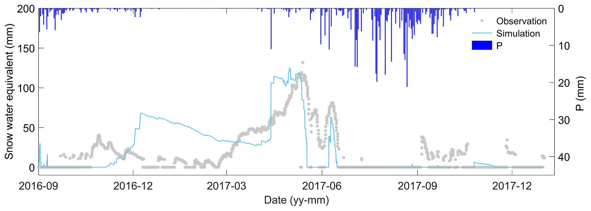
Figure B1Time series of the observed and estimated snow water equivalent using the developed STEMMUS-UEB model.
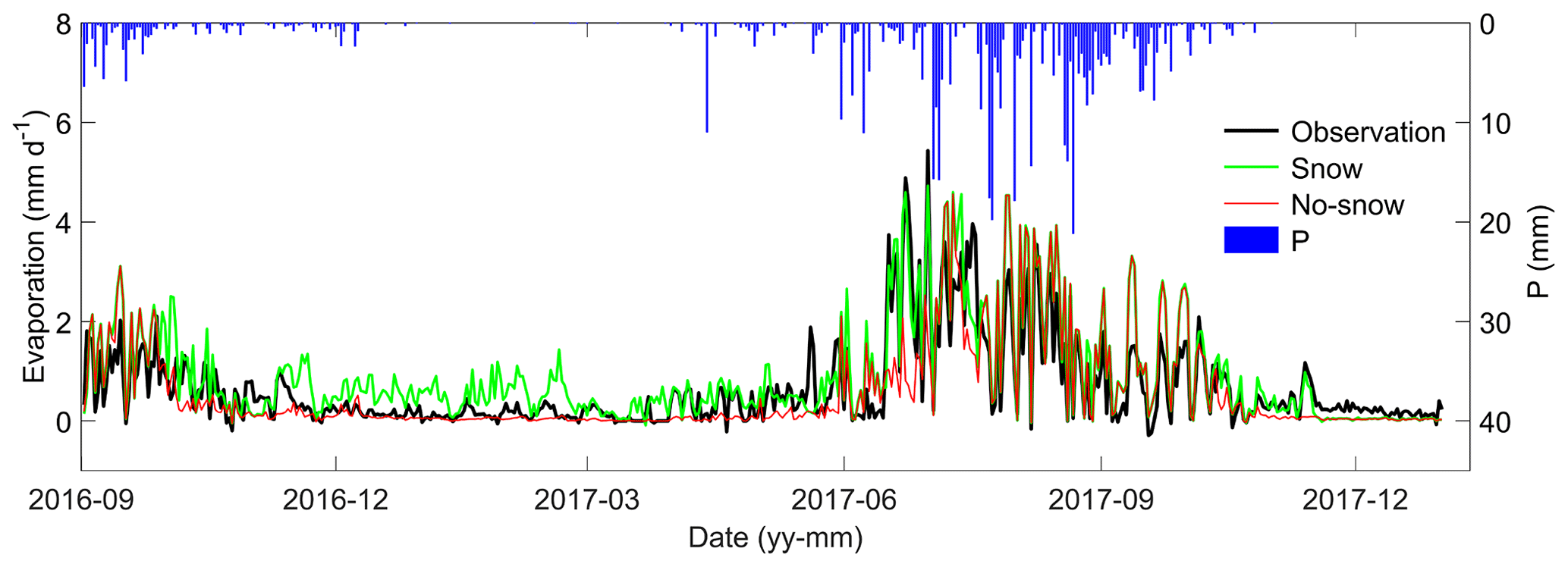
Figure B2Intercomparison of the observed and estimated surface evaporation using the model with and without the snow module.

Figure B3Measured and estimated daily surface evaporation using the model with and without snow module (a and b, respectively).
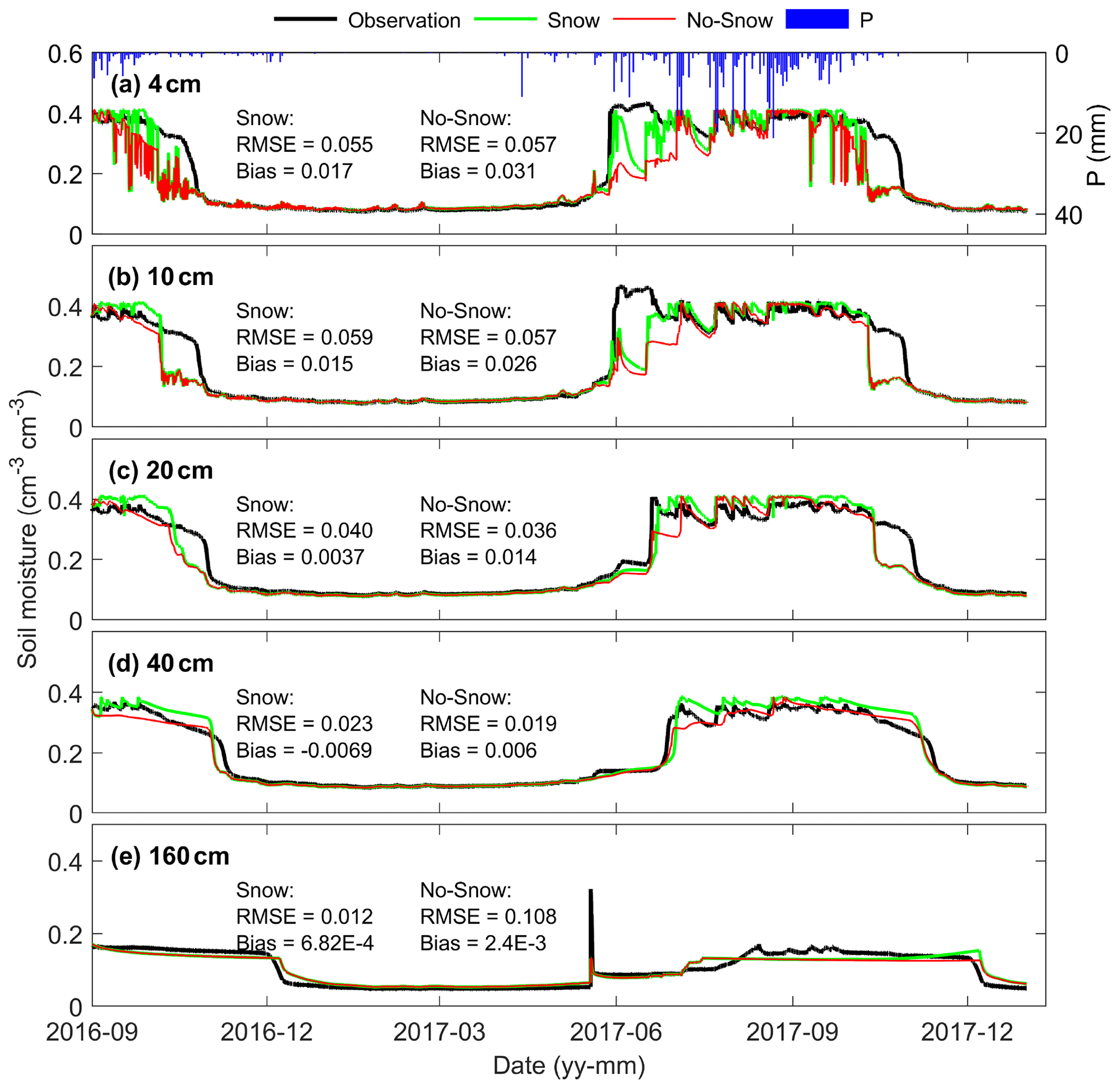
Figure B4Observed and estimated soil moisture at various soil layers using the model with and without the snow module.
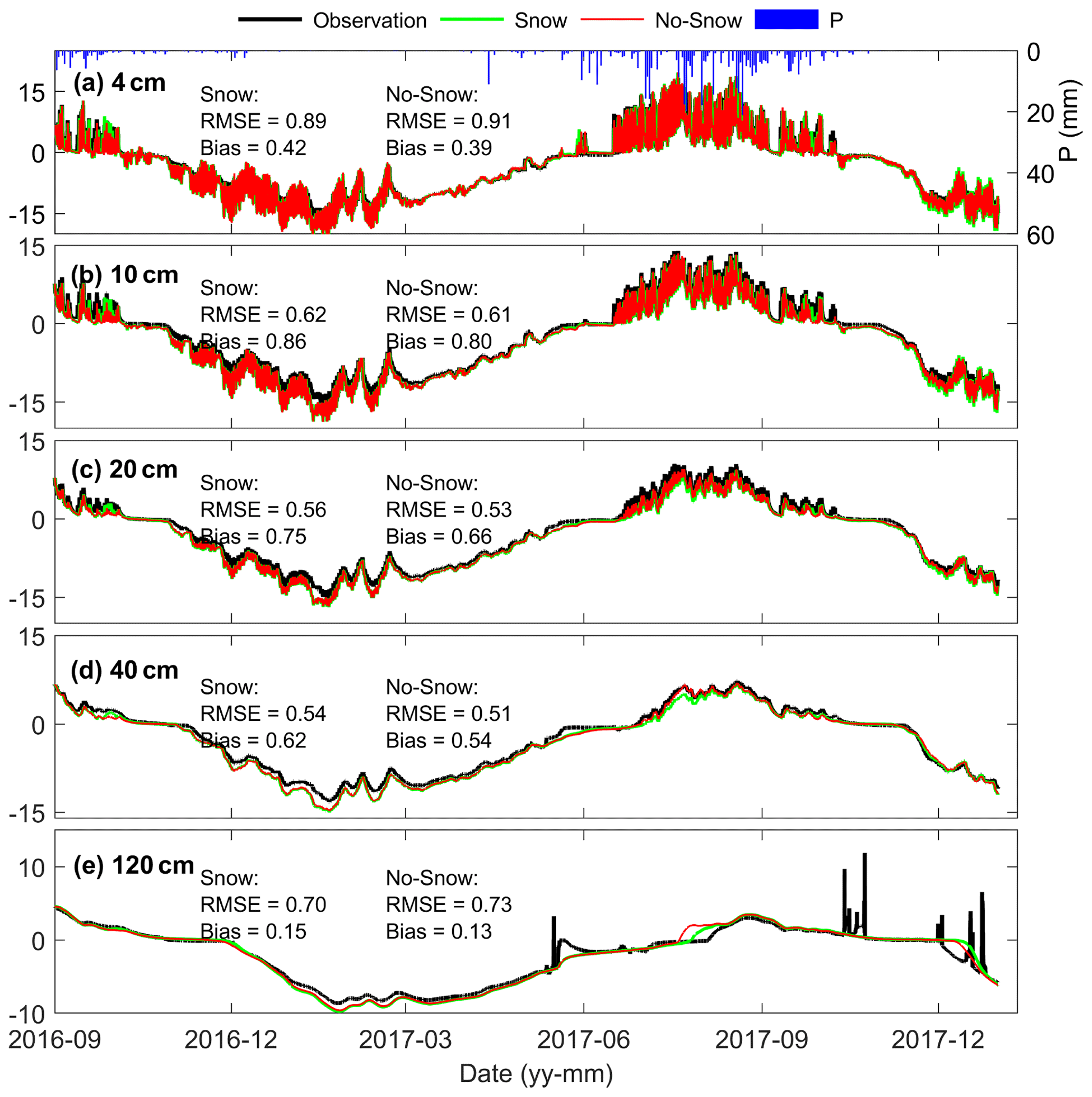
Figure B5Observed and estimated soil temperature at various soil layers using the model with and without the snow module.

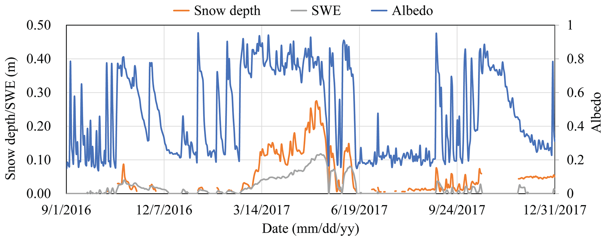
Figure B7Time series of the snow depth, snow water equivalent (SWE), and albedo (Yakou station).
The coupled soil–snow model (STEMMUS-UEB v1.0.0) with three levels of complexity of soil water and heat transfer physics was developed based on the STEMMUS-FT (Simultaneous Transfer of Energy, Momentum and Mass in Unsaturated Soils with Freeze and Thaw) and UEB (Utah energy balance) models. The original STEMMUS source code is available from the GitHub website via https://github.com/yijianzeng/STEMMUS (Zeng and Su, 2020). The snowmelt module is based on the code of Tarboton and Luce (1996). The coupled STEMMUS-UEB v1.0.0 code is archived on Zenodo (https://doi.org/10.5281/zenodo.3975846, Yu et al., 2020b), licensed under the Apache License, version 2.0. The current code is tested by MATLAB 2019b using an Intel Core i7 processor (Intel® Core™ i7-6700HQ CPU @ 2.60 GHz 2.59 GHz), an installed memory (RAM, 16.0 GB), and a 64-bit Windows 10 Enterprise operating system. The relevant data can be accessed from 4TU.ResearchData (https://doi.org/10.4121/uuid:cc69b7f2-2448-4379-b638-09327012ce9b, Yu et al., 2018b; https://doi.org/10.4121/uuid:c712717c-6ac0-47ff-9d58-97f88082ddc0, Zhao et al., 2018b, for Maqu the case) and the Cold and Arid Regions Science Data Center at Lanzhou (https://doi.org/10.3972/hiwater.001.2019.db, Li, 2019, for the Yakou case).
The supplement related to this article is available online at: https://doi.org/10.5194/gmd-14-7345-2021-supplement.
ZS, YZ, and LY designed and conceptualized this study. YZ and ZS provided the original version of STEMMUS model code and supervised the further modeling development. LY developed the STEMMUS-UEB model coupling framework with contributions from YZ. LY and YZ prepared the original draft of the paper. LY, YZ, and ZS all contributed to the reviewing and editing of the final paper.
The contact author has declared that neither they nor their co-authors have any competing interests.
Publisher's note: Copernicus Publications remains neutral with regard to jurisdictional claims in published maps and institutional affiliations.
The authors thank the editors and referees very much for their constructive comments and suggestions for improving the manuscript.
This research has been supported by the National Natural Science Foundation of China (grant no. 41971033) and the Fundamental Research Funds for the Central Universities (CHD; grant no. 300102298307).
This paper was edited by Heiko Goelzer and reviewed by three anonymous referees.
Barlett, P. A., MacKay, M. D., and Verseghy, D. L.: Modified snow algorithms in the Canadian Land Surface Scheme: Model runs and sensitivity analysis at three boreal forest stands, Atmos. Ocean, 44, 207–222, https://doi.org/10.3137/ao.440301, 2006.
Barrere, M., Domine, F., Decharme, B., Morin, S., Vionnet, V., and Lafaysse, M.: Evaluating the performance of coupled snow–soil models in SURFEXv8 to simulate the permafrost thermal regime at a high Arctic site, Geosci. Model Dev., 10, 3461–3479, https://doi.org/10.5194/gmd-10-3461-2017, 2017.
Best, M. J., Pryor, M., Clark, D. B., Rooney, G. G., Essery, R. L. H., Ménard, C. B., Edwards, J. M., Hendry, M. A., Porson, A., Gedney, N., Mercado, L. M., Sitch, S., Blyth, E., Boucher, O., Cox, P. M., Grimmond, C. S. B., and Harding, R. J.: The Joint UK Land Environment Simulator (JULES), model description – Part 1: Energy and water fluxes, Geosci. Model Dev., 4, 677–699, https://doi.org/10.5194/gmd-4-677-2011, 2011.
Bittelli, M., Ventura, F., Campbell, G. S., Snyder, R. L., Gallegati, F., and Pisa, P. R.: Coupling of heat, water vapor, and liquid water fluxes to compute evaporation in bare soils, J. Hydrol., 362, 191–205, https://doi.org/10.1016/j.jhydrol.2008.08.014, 2008.
Boone, A., Samuelsson, P., Gollvik, S., Napoly, A., Jarlan, L., Brun, E., and Decharme, B.: The interactions between soil–biosphere–atmosphere land surface model with a multi-energy balance (ISBA-MEB) option in SURFEXv8 – Part 1: Model description, Geosci. Model Dev., 10, 843–872, https://doi.org/10.5194/gmd-10-843-2017, 2017.
Boone, A. A. and Etchevers, P.: An intercomparison of three snow schemes of varying complexity coupled to the same land surface model: Local-scale evaluation at an alpine site, J. Hydrometeorol., 2, 374-394, https://doi.org/10.1175/1525-7541(2001)002<0374:AIOTSS>2.0.CO;2, 2001.
Che, T., Li, X., Liu, S., Li, H., Xu, Z., Tan, J., Zhang, Y., Ren, Z., Xiao, L., Deng, J., Jin, R., Ma, M., Wang, J., and Yang, X.: Integrated hydrometeorological, snow and frozen-ground observations in the alpine region of the Heihe River Basin, China, Earth Syst. Sci. Data, 11, 1483–1499, https://doi.org/10.5194/essd-11-1483-2019, 2019.
Cuntz, M. and Haverd, V.: Physically Accurate Soil Freeze-Thaw Processes in a Global Land Surface Scheme, J. Adv. Model. Earth Sy., 10, 54–77, https://doi.org/10.1002/2017ms001100, 2018.
Dall'Amico, M., Endrizzi, S., Gruber, S., and Rigon, R.: A robust and energy-conserving model of freezing variably-saturated soil, The Cryosphere, 5, 469–484, https://doi.org/10.5194/tc-5-469-2011, 2011.
Decharme, B., Brun, E., Boone, A., Delire, C., Le Moigne, P., and Morin, S.: Impacts of snow and organic soils parameterization on northern Eurasian soil temperature profiles simulated by the ISBA land surface model, The Cryosphere, 10, 853–877, https://doi.org/10.5194/tc-10-853-2016, 2016.
Dente, L., Vekerdy, Z., Wen, J., and Su, Z.: Maqu network for validation of satellite-derived soil moisture products, Int. J. Appl. Earth Obs. Geoinf., 17, 55–65, https://doi.org/10.1016/j.jag.2011.11.004, 2012.
De Vries, D. A.: Simultaneous transfer of heat and moisture in porous media, Eos T. Am. Geophys. Un. 39, 909–916, https://doi.org/10.1029/TR039i005p00909, 1958.
Dickinson, R. E., Henderson-Sellers, A., and Kennedy, P. J.: Biosphere-atmosphere Transfer Scheme (BATS) Version 1e as Coupled to the NCAR Community Climate Model (No. NCAR/TN-387+STR), University Corporation for Atmospheric Research, 1993.
Ding, B., Yang, K., Qin, J., Wang, L., Chen, Y., and He, X.: The dependence of precipitation types on surface elevation and meteorological conditions and its parameterization, J. Hydrol., 513, 154–163, https://doi.org/10.1016/j.jhydrol.2014.03.038, 2014.
Ding, B., Yang, K., Yang, W., He, X., Chen, Y., Lazhu, Guo, X., Wang, L., Wu, H., and Yao, T.: Development of a Water and Enthalpy Budget-based Glacier mass balance Model (WEB-GM) and its preliminary validation, Water Resour. Res., 53, 3146–3178, https://doi.org/10.1002/2016WR018865, 2017.
Domine, F., Picard, G., Morin, S., Barrere, M., Madore, J.-B., and Langlois, A.: Major Issues in Simulating Some Arctic Snowpack Properties Using Current Detailed Snow Physics Models: Consequences for the Thermal Regime and Water Budget of Permafrost, J. Adv. Model. Earth Sy., 11, 34–44, https://doi.org/10.1029/2018ms001445, 2019.
Douville, H., Royer, J. F., and Mahfouf, J. F.: A new snow parameterization for the Météo-France climate model, Clim. Dynam., 12, 21–35, https://doi.org/10.1007/BF00208760, 1995.
Dutra, E., Balsamo, G., Viterbo, P., Miranda, P. M. A., Beljaars, A., Schar, C., and Elder, K.: An improved snow scheme for the ECMWF land surface model: Description and offline validation, J. Hydrometeorol., 11, 899–916, https://doi.org/10.1175/2010JHM1249.1, 2010.
Dutra, E., Viterbo, P., Miranda, P. M. A., and Balsamo, G.: Complexity of snow schemes in a climate model and its impact on surface energy and hydrology, J. Hydrometeorol., 13, 521–538, https://doi.org/10.1175/JHM-D-11-072.1, 2012.
Ekici, A., Beer, C., Hagemann, S., Boike, J., Langer, M., and Hauck, C.: Simulating high-latitude permafrost regions by the JSBACH terrestrial ecosystem model, Geosci. Model Dev., 7, 631–647, https://doi.org/10.5194/gmd-7-631-2014, 2014.
Etchevers, P., Martin, E., Brown, R., Fierz, C., Lejeune, Y., Bazile, E., Boone, A., Dai, Y.-J., Essery, R., Fernandez, A., Gusev, Y., Jordan, R., Koren, V., Kowalczyk, E., Nasonova, N. O., Pyles, R. D., Schlosser, A., Shmakin, A. B., Smirnova, T. G., Strasser, U., Verseghy, D., Yamazaki, T., and Yang, Z.-L.: Validation of the energy budget of an alpine snowpack simulated by several snow models (SnowMIP project), Ann. Glaciol., 38, 150–158, https://doi.org/10.3189/172756404781814825, 2004.
Flerchinger, G. N.: The Simultaneous Heat and Water (SHAW) Model: Technical Documentation Version 3.0, Northwest Watershed Research Center, USDA Agricultural Research Service, Boise, Idaho, USA, Technical Rep., 43 pp., 2017.
Flerchinger, G. N. and Saxton, K. E.: Simultaneous heat and water model of a freezing snow-residue-soil system. I. Theory and development, T. Am. Soc. Agr. Eng., 32, 565–571, 1989.
Gardiner, M. J., Ellis-Evans, J. C., Anderson, M. G., and Tranter, M.: Snowmelt modelling on Signy Island, South Orkney Islands, Ann. Glaciol., 26, 161–166, https://doi.org/10.3189/1998aog26-1-161-166, 1998.
Gichamo, T. Z. and Tarboton, D. G.: Ensemble Streamflow Forecasting Using an Energy Balance Snowmelt Model Coupled to a Distributed Hydrologic Model with Assimilation of Snow and Streamflow Observations, Water Resour. Res., 55, 10813–10838, https://doi.org/10.1029/2019wr025472, 2019.
Günther, D., Marke, T., Essery, R., and Strasser, U.: Uncertainties in Snowpack Simulations – Assessing the Impact of Model Structure, Parameter Choice, and Forcing Data Error on Point-Scale Energy Balance Snow Model Performance, Water Resour. Res., 55, 2779–2800, https://doi.org/10.1029/2018wr023403, 2019.
Gusev, Y. M. and Nasonova, O. N.: The simulation of heat and water exchange in the boreal spruce forest by the land-surf ace model SWAP, J. Hydrol., 280, 162–191, https://doi.org/10.1016/S0022-1694(03)00221-X, 2003.
Hagedorn, B., Sletten, R. S., and Hallet, B.: Sublimation and ice condensation in hyperarid soils: Modeling results using field data from Victoria Valley, Antarctica, J. Geophys. Res.-Earth, 112, F03017, https://doi.org/10.1029/2006jf000580, 2007.
Hansson, K., Šimůnek, J., Mizoguchi, M., Lundin, L. C., and van Genuchten, M. T.: Water flow and heat transport in frozen soil: Numerical solution and freeze-thaw applications, Vadose Zone J., 3, 693–704, 2004.
Harder, P. and Pomeroy, J. W.: Hydrological model uncertainty due to precipitation-phase partitioning methods, Hydrol. Process., 28, 4311–4327, https://doi.org/10.1002/hyp.10214, 2014.
Hrbáček, F., Láska, K., and Engel, Z.: Effect of snow cover on the active-layer thermal regime – a case study from James Ross island, Antarctic Peninsula, Permafrost Periglac., 27, 307–315, 2016.
Iwata, Y., Hayashi, M., Suzuki, S., Hirota, T., and Hasegawa, S.: Effects of snow cover on soil freezing, water movement, and snowmelt infiltration: A paired plot experiment, Water Resour. Res., 46, W09504, https://doi.org/10.1029/2009WR008070, 2010.
Jambon-Puillet, E., Shahidzadeh, N., and Bonn, D.: Singular sublimation of ice and snow crystals, Nat. Commun., 9, 4191, https://doi.org/10.1038/s41467-018-06689-x, 2018.
Jansson, P. E.: CoupModel: Model Use, Calibration, and Validation, T. ASABE, 55, 1337, https://doi.org/10.13031/2013.42245, 2012.
Jordan, R.: A one-dimensional temperature model for a snow cover: Technical documentation for SNTHERM. 89, Cold Regions Research and Engineering Lab Hanover NH, 1991.
Koren, V., Schaake, J., Mitchell, K., Duan, Q. Y., Chen, F., and Baker, J. M.: A parameterization of snowpack and frozen ground intended for NCEP weather and climate models, J. Geophys. Res.-Atmos., 104, 19569–19585, https://doi.org/10.1029/1999JD900232, 1999.
Lawrence, D. M., Fisher, R. A., Koven, C. D., Oleson, K. W., Swenson, S. C., Bonan, G., Collier, N., Ghimire, B., van Kampenhout, L., Kennedy, D., Kluzek, E., Lawrence, P. J., Li, F., Li, H., Lombardozzi, D., Riley, W. J., Sacks, W. J., Shi, M., Vertenstein, M., Wieder, W. R., Xu, C., Ali, A. A., Badger, A. M., Bisht, G., van den Broeke, M., Brunke, M. A., Burns, S. P., Buzan, J., Clark, M., Craig, A., Dahlin, K., Drewniak, B., Fisher, J. B., Flanner, M., Fox, A. M., Gentine, P., Hoffman, F., Keppel-Aleks, G., Knox, R., Kumar, S., Lenaerts, J., Leung, L. R., Lipscomb, W. H., Lu, Y., Pandey, A., Pelletier, J. D., Perket, J., Randerson, J. T., Ricciuto, D. M., Sanderson, B. M., Slater, A., Subin, Z. M., Tang, J., Thomas, R. Q., Val Martin, M., and Zeng, X.: The Community Land Model Version 5: Description of New Features, Benchmarking, and Impact of Forcing Uncertainty, J. Adv. Model. Earth Sy., 11, 4245–4287, https://doi.org/10.1029/2018MS001583, 2019.
Lehning, M., Bartelt, P., Brown, B., Russi, T., Stöckli, U., and Zimmerli, M.: SNOWPACK model calculations for avalanche warning based upon a new network of weather and snow stations, Cold Reg. Sci. Technol., 30, 145–157, https://doi.org/10.1016/S0165-232X(99)00022-1, 1999.
Leroux, N. R. and Pomeroy, J. W.: Modelling capillary hysteresis effects on preferential flow through melting and cold layered snowpacks, Adv. Water Resour., 107, 250–264, https://doi.org/10.1016/j.advwatres.2017.06.024, 2017.
Li, D., Wen, L., Long, X., and Chen, S.: Observation Study on Effects of Snow Cover on Local Micro Meteorological Characteristics in Maqu, Plateau Meteorol., 36, 330–339, https://doi.org/10.7522/j.issn.1000-0534.2016.00074, 2017.
Li, H., Li, X., Yang, D., Wang, J., Gao, B., Pan, X., Zhang, Y., and Hao, X.: Tracing Snowmelt Paths in an Integrated Hydrological Model for Understanding Seasonal Snowmelt Contribution at Basin Scale, J. Geophys. Res.-Atmos., 124, 8874–8895, https://doi.org/10.1029/2019JD030760, 2019.
Li, X.: Integrated hydrometeorological – snow – frozen ground observations in the alpine region of the Heihe River Basin, China, Cold and Arid Regions Science Data Center at Lanzhou (CARD) [data set], https://doi.org/10.3972/hiwater.001.2019.db, 2019.
Mahat, V. and Tarboton, D. G.: Representation of canopy snow interception, unloading and melt in a parsimonious snowmelt model, Hydrol. Process., 28, 6320–6336, https://doi.org/10.1002/hyp.10116, 2014.
Milly, P. C. D.: Moisture and heat transport in hysteretic, inhomogeneous porous media: A matric head-based formulation and a numerical model, Water Resour. Res., 18, 489–498, https://doi.org/10.1029/WR018i003p00489, 1982.
Mualem, Y.: A new model for predicting the hydraulic conductivity of unsaturated porous media, Water Resour. Res., 12, 513–522, https://doi.org/10.1029/WR012i003p00513, 1976.
Niu, G. Y., Yang, Z. L., Mitchell, K. E., Chen, F., Ek, M. B., Barlage, M., Kumar, A., Manning, K., Niyogi, D., Rosero, E., Tewari, M., and Xia, Y.: The community Noah land surface model with multiparameterization options (Noah-MP): 1. Model description and evaluation with local-scale measurements, J. Geophys. Res.-Atmos., 116, D12109, https://doi.org/10.1029/2010JD015139, 2011.
Painter, S. L., Coon, E. T., Atchley, A. L., Berndt, M., Garimella, R., Moulton, J. D., Svyatskiy, D., and Wilson, C. J.: Integrated surface/subsurface permafrost thermal hydrology: Model formulation and proof-of-concept simulations, Water Resour. Res., 52, 6062–6077, https://doi.org/10.1002/2015WR018427, 2016.
Pan, X., Helgason, W., Ireson, A., and Wheater, H.: Field-scale water balance closure in seasonally frozen conditions, Hydrol Earth Syst Sci, 21, 5401-5413, https://doi.org/10.5194/hess-21-5401-2017, 2017.
Pimentel, R., Herrero, J., Zeng, Y., Su, Z., and Polo, M. J.: Study of Snow Dynamics at Subgrid Scale in Semiarid Environments Combining Terrestrial Photography and Data Assimilation Techniques, J. Hydrometeorol., 16, 563–578, https://doi.org/10.1175/jhm-d-14-0046.1, 2015.
Pitman, A. J., Yang, Z.-L., Cogley, J. G., and Henderson-Sellers, A.: Description of bare essentials of surface transfer for the Bureau of Meteorology Research Centre AGCM, Macquarie University, North Ryde, NSW, Australia, BMRC Res. Rep., 117 pp., 1991.
Prunty, L. and Bell, J.: Infiltration rate vs. gas composition and pressure in soil columns, Soil Sci. Soc. Am. J., 71, 1473–1475, https://doi.org/10.2136/sssaj2007.0072N, 2007.
Richards, L. A.: Capillary Conduction of Liquids Through Porous Mediums, Physics, 1, 318–333, https://doi.org/10.1063/1.1745010, 1931.
Rutter, N., Essery, R., Pomeroy, J., Altimir, N., Andreadis, K., Baker, I., Barr, A., Bartlett, P., Boone, A., Deng, H., Douville, H., Dutra, E., Elder, K., Ellis, C., Feng, X., Gelfan, A., Goodbody, A., Gusev, Y., Gustafsson, D., Hellström, R., Hirabayashi, Y., Hirota, T., Jonas, T., Koren, V., Kuragina, A., Lettenmaier, D., Li, W.-P., Luce, C., Martin, E., Nasonova, O., Pumpanen, J., Pyles, R. D., Samuelsson, P., Sandells, M., Schädler, G., Shmakin, A., Smirnova, T. G., Stähli, M., Stöckli, R., Strasser, U., Su, H., Suzuki, K., Takata, K., Tanaka, K., Thompson, E., Vesala, T., Viterbo, P., Wiltshire, A., Xia, K., Xue, Y., and Yamazaki, T.: Evaluation of forest snow processes models (SnowMIP2), J. Geophys. Res.-Atmos., 114, D06111, https://doi.org/10.1029/2008JD011063, 2009.
Scanlon, B. R. and Milly, P. C. D.: Water and heat fluxes in desert soils: 2. Numerical simulations, Water Resour. Res., 30, 721–733, https://doi.org/10.1029/93WR03252, 1994.
Schulz, O. and de Jong, C.: Snowmelt and sublimation: field experiments and modelling in the High Atlas Mountains of Morocco, Hydrol. Earth Syst. Sci., 8, 1076–1089, https://doi.org/10.5194/hess-8-1076-2004, 2004.
Shrestha, M., Wang, L., Koike, T., Xue, Y., and Hirabayashi, Y.: Improving the snow physics of WEB-DHM and its point evaluation at the SnowMIP sites, Hydrol. Earth Syst. Sci., 14, 2577–2594, https://doi.org/10.5194/hess-14-2577-2010, 2010.
Šimůnek, J., Šejna, M., Saito, H., Sakai, M., and Van Genuchten, M.: The HYDRUS-1D Software Package for Simulating the One-Dimensional Movement of Water, Heat, and Multiple Solutes in Variably-Saturated Media, University of California Riverside, Riverside, California, USA, 330 pp., 2008.
Slater, A. G., Pitman, A. J., and Desborough, C. E.: The validation of a snow parameterization designed for use in general circulation models, Int. J. Climatol., 18, 595–617, https://doi.org/10.1002/(sici)1097-0088(199805)18:6<595::aid-joc275>3.0.co;2-o, 1998.
Strasser, U., Bernhardt, M., Weber, M., Liston, G. E., and Mauser, W.: Is snow sublimation important in the alpine water balance?, The Cryosphere, 2, 53–66, https://doi.org/10.5194/tc-2-53-2008, 2008.
Su, Z., Wen, J., Dente, L., van der Velde, R., Wang, L., Ma, Y., Yang, K., and Hu, Z.: The Tibetan Plateau observatory of plateau scale soil moisture and soil temperature (Tibet-Obs) for quantifying uncertainties in coarse resolution satellite and model products, Hydrol. Earth Syst. Sci., 15, 2303–2316, https://doi.org/10.5194/hess-15-2303-2011, 2011.
Su, Z., De Rosnay, P., Wen, J., Wang, L., and Zeng, Y.: Evaluation of ECMWF's soil moisture analyses using observations on the Tibetan Plateau, J. Geophys. Res.-Atmos., 118, 5304–5318, https://doi.org/10.1002/jgrd.50468, 2013.
Sud, Y. C. and Mocko, D. M.: New Snow-Physics to Complement SSiB Part I: Design and Evaluation with ISLSCP Initiative I Datasets, J. Meteorol. Soc. Jpn. Ser. II, 77, 335–348, https://doi.org/10.2151/jmsj1965.77.1B_335, 1999.
Sultana, R., Hsu, K.-L., Li, J., and Sorooshian, S.: Evaluating the Utah Energy Balance (UEB) snow model in the Noah land-surface model, Hydrol. Earth Syst. Sci., 18, 3553–3570, https://doi.org/10.5194/hess-18-3553-2014, 2014.
Sun, S., Jin, J., and Xue, Y.: A simple snow-atmosphere-soil transfer model, J. Geophys. Res.-Atmos., 104, 19587–19597, https://doi.org/10.1029/1999jd900305, 1999.
Swenson, S. C., Lawrence, D. M., and Lee, H.: Improved simulation of the terrestrial hydrological cycle in permafrost regions by the Community Land Model, J. Adv. Model. Earth Sy., 4, M08002, https://doi.org/10.1029/2012MS000165, 2012.
Tarboton, D. G. and Luce, C. H.: Utah Energy Balance Snow Accumulation and Melt Model (UEB), Computer model technical description and users guide, Utah Water Research Laboratory and USDA Forest Service Intermountain Research Station, Logan, Utah, USA, Rep., 64 pp., 1996.
Touma, J. and Vauclin, M.: Experimental and numerical analysis of two-phase infiltration in a partially saturated soil, Transp. Porous Media, 1, 27–55, https://doi.org/10.1007/BF01036524, 1986.
Ueno, K., Tanaka, K., Tsutsui, H., and Li, M.: Snow Cover Conditions in the Tibetan Plateau Observed during the Winter of 2003/2004, Arct. Antarct. Alp. Res., 39, 152–164, https://doi.org/10.1657/1523-0430(2007)39[152:SCCITT]2.0.CO;2, 2007.
Ueno, K., Sugimoto, S., Tsutsui, H., Taniguchi, K., Hu, Z., and Wu, S.: Role of patchy snow cover on the planetary boundary layer structure during late winter observed in the central Tibetan Plateau, J. Meteorol. Soc. Jpn. Ser. II, 90, 145–155, 2012.
van Genuchten, M. T.: A closed-form equation for predicting the hydraulic conductivity of unsaturated soils, Soil Sci. Soc. Am. J., 44, 892–898, https://doi.org/10.2136/SSSAJ1980.03615995004400050002X, 1980.
Verseghy, D. L.: Class – A Canadian land surface scheme for GCMS. I. Soil model, Int. J. Climatol., 11, 111–133, https://doi.org/10.1002/joc.3370110202, 1991.
Vionnet, V., Brun, E., Morin, S., Boone, A., Faroux, S., Le Moigne, P., Martin, E., and Willemet, J.-M.: The detailed snowpack scheme Crocus and its implementation in SURFEX v7.2, Geosci. Model Dev., 5, 773–791, https://doi.org/10.5194/gmd-5-773-2012, 2012.
Wang, L., Koike, T., Yang, D., and Yang, K.: Improving the hydrology of the Simple Biosphere Model 2 and its evaluation within the framework of a distributed hydrological model, Hydrol. Sci. J., 54, 989–1006, https://doi.org/10.1623/hysj.54.6.989, 2009.
Wang, L., Zhou, J., Qi, J., Sun, L., Yang, K., Tian, L., Lin, Y., Liu, W., Shrestha, M., Xue, Y., Koike, T., Ma, Y., Li, X., Chen, Y., Chen, D., Piao, S., and Lu, H.: Development of a land surface model with coupled snow and frozen soil physics, Water Resour. Res., 53, 5085–5103, https://doi.org/10.1002/2017WR020451, 2017.
Wang, T., Ottlé, C., Boone, A., Ciais, P., Brun, E., Morin, S., Krinner, G., Piao, S., and Peng, S.: Evaluation of an improved intermediate complexity snow scheme in the ORCHIDEE land surface model, J. Geophys. Res.-Atmos., 118, 6064–6079, https://doi.org/10.1002/jgrd.50395, 2013.
Wang, Y., Zeng, Y., Yu, L., Yang, P., Van der Tol, C., Yu, Q., Lü, X., Cai, H., and Su, Z.: Integrated modeling of canopy photosynthesis, fluorescence, and the transfer of energy, mass, and momentum in the soil–plant–atmosphere continuum (STEMMUS–SCOPE v1.0.0), Geosci. Model Dev., 14, 1379–1407, https://doi.org/10.5194/gmd-14-1379-2021, 2021.
Watson, F. G. R., Newman, W. B., Coughlan, J. C., and Garrott, R. A.: Testing a distributed snowpack simulation model against spatial observations, J. Hydrol., 328, 453–466, https://doi.org/10.1016/j.jhydrol.2005.12.012, 2006.
Wicky, J. and Hauck, C.: Numerical modelling of convective heat transport by air flow in permafrost talus slopes, The Cryosphere, 11, 1311–1325, https://doi.org/10.5194/tc-11-1311-2017, 2017.
Yang, Z.-L., Dickinson, R. E., Robock, A., and Vinnikov, K. Y.: Validation of the Snow Submodel of the Biosphere–Atmosphere Transfer Scheme with Russian Snow Cover and Meteorological Observational Data, J. Climate, 10, 353–373, https://doi.org/10.1175/1520-0442(1997)010<0353:votsso>2.0.co;2, 1997.
Yi, Y., Kimball, J. S., Rawlins, M. A., Moghaddam, M., and Euskirchen, E. S.: The role of snow cover affecting boreal-arctic soil freeze–thaw and carbon dynamics, Biogeosciences, 12, 5811–5829, https://doi.org/10.5194/bg-12-5811-2015, 2015.
You, Y., Meng, H., Dong, J., and Rudlosky, S.: Time-Lag Correlation Between Passive Microwave Measurements and Surface Precipitation and Its Impact on Precipitation Retrieval Evaluation, Geophys. Res. Lett., 46, 8415–8423, https://doi.org/10.1029/2019gl083426, 2019.
Yu, L., Zeng, Y., Su, Z., Cai, H., and Zheng, Z.: The effect of different evapotranspiration methods on portraying soil water dynamics and ET partitioning in a semi-arid environment in Northwest China, Hydrol. Earth Syst. Sci., 20, 975–990, https://doi.org/10.5194/hess-20-975-2016, 2016.
Yu, L., Zeng, Y., Wen, J., and Su, Z.: Liquid-Vapor-Air Flow in the Frozen Soil, J. Geophys. Res.-Atmos., 123, 7393–7415, https://doi.org/10.1029/2018jd028502, 2018a.
Yu, L., Zeng, Y., Su, Z., and Wen, J.: HydroThermal Dynamics of Frozen Soils on the Tibetan Plateau during 2015–2016, 4TU.ResearchData [data set], https://doi.org/10.4121/uuid:cc69b7f2-2448-4379-b638-09327012ce9b, 2018b.
Yu, L., Fatichi, S., Zeng, Y., and Su, Z.: The role of vadose zone physics in the ecohydrological response of a Tibetan meadow to freeze–thaw cycles, The Cryosphere, 14, 4653–4673, https://doi.org/10.5194/tc-14-4653-2020, 2020a.
Yu, L., Zeng, Y., and Su, Z.: STEMMUS-UEB v1.0: Integrated Modeling of Snowpack and Soil Mass and Energy Transfer with Three Levels of Soil Physical Process Complexities, Zenodo [code], https://doi.org/10.5281/zenodo.3975846, 2020b.
Yu, L., Zeng, Y., and Su, Z.: Understanding the mass, momentum, and energy transfer in the frozen soil with three levels of model complexities, Hydrol. Earth Syst. Sci., 24, 4813–4830, https://doi.org/10.5194/hess-24-4813-2020, 2020c.
Zeng, Y. and Su, Z.: STEMMUS source code, GitHub [code], available at: https://github.com/yijianzeng/STEMMUS, last access: 11 December 2020.
Zeng, Y., Su, Z., Wan, L., Yang, Z., Zhang, T., Tian, H., Shi, X., Wang, X., and Cao, W.: Diurnal pattern of the drying front in desert and its application for determining the effective infiltration, Hydrol. Earth Syst. Sci., 13, 703–714, https://doi.org/10.5194/hess-13-703-2009, 2009a.
Zeng, Y., Wan, L., Su, Z., Saito, H., Huang, K., and Wang, X.: Diurnal soil water dynamics in the shallow vadose zone (field site of China University of Geosciences, China), Environ. Geol., 58, 11–23, https://doi.org/10.1007/s00254-008-1485-8, 2009b.
Zeng, Y., Su, Z., Wan, L., and Wen, J.: Numerical analysis of air-water-heat flow in unsaturated soil: Is it necessary to consider airflow in land surface models?, J. Geophys. Res.-Atmos., 116, D20107, https://doi.org/10.1029/2011JD015835, 2011a.
Zeng, Y., Su, Z., Wan, L., and Wen, J.: A simulation analysis of the advective effect on evaporation using a two-phase heat and mass flow model, Water Resour. Res., 47, W10529, https://doi.org/10.1029/2011WR010701, 2011b.
Zeng, Y., Su, Z., van der Velde, R., Wang, L., Xu, K., Wang, X., and Wen, J.: Blending Satellite Observed, Model Simulated, and in Situ Measured Soil Moisture over Tibetan Plateau, Remote Sensing, 8, 268, https://doi.org/10.3390/rs8030268, 2016.
Zeng, Y. J. and Su, Z. B.: STEMMUS: Simultaneous Transfer of Engery, Mass and Momentum in Unsaturated Soil,University of Twente, Faculty of Geo-Information and Earth Observation (ITC), Enschede, ISBN: 978-90-6164-351-7, 2013.
Zhang, T.: Influence of the seasonal snow cover on the ground thermal regime: An overview, Rev. Geophys., 43, RG4002, https://doi.org/10.1029/2004rg000157, 2005.
Zhao, H., Zeng, Y., Lv, S., and Su, Z.: Analysis of soil hydraulic and thermal properties for land surface modeling over the Tibetan Plateau, Earth Syst. Sci. Data, 10, 1031–1061, https://doi.org/10.5194/essd-10-1031-2018, 2018a.
Zhao, H., Zeng, Y., and Su, Z.: Soil Hydraulic and Thermal Properties for Land Surface Modelling over the Tibetan Plateau, 4TU.ResearchData [data set], https://doi.org/10.4121/uuid:c712717c-6ac0-47ff-9d58-97f88082ddc0, 2018b.
Zheng, D., Van der Velde, R., Su, Z., Wang, X., Wen, J., Booij, M. J., Hoekstra, A. Y., and Chen, Y.: Augmentations to the Noah Model Physics for Application to the Yellow River Source Area. Part I: Soil Water Flow, J. Hydrometeorol., 16, 2659–2676, https://doi.org/10.1175/JHM-D-14-0198.1, 2015.
- Abstract
- Introduction
- Description of the coupled soil–snow modeling framework and model setup
- Results: comparison of simulation results of surface variables with and without snowpack effect
- Discussion
- Conclusions
- Appendix A
- Appendix B
- Code and data availability
- Author contributions
- Competing interests
- Disclaimer
- Acknowledgements
- Financial support
- Review statement
- References
- Supplement