the Creative Commons Attribution 4.0 License.
the Creative Commons Attribution 4.0 License.
 | 30 Nov 2021
Explicit silicate cycling in the Kiel Marine Biogeochemistry Model version 3 (KMBM3) embedded in the UVic ESCM version 2.9
David P. Keller
Wolfgang Koeve
Katrin J. Meissner
Christopher J. Somes
Wanxuan Yao
Andreas Oschlies
We describe and test a new model of biological marine silicate cycling, implemented in the Kiel Marine Biogeochemical Model version 3 (KMBM3), embedded in the University of Victoria Earth System Climate Model (UVic ESCM) version 2.9. This new model adds diatoms, which are a key component of the biological carbon pump, to an existing ecosystem model. This new model combines previously published parameterizations of a diatom functional type, opal production and export with a novel, temperature-dependent dissolution scheme. Modelled steady-state biogeochemical rates, carbon and nutrient distributions are similar to those found in previous model versions. The new model performs well against independent ocean biogeochemical indicators and captures the large-scale features of the marine silica cycle to a degree comparable to similar Earth system models. Furthermore, it is computationally efficient, allowing both fully coupled, long-timescale transient simulations and “offline” transport matrix spinups. We assess the fully coupled model against modern ocean observations, the historical record starting from 1960 and a business-as-usual atmospheric CO2 forcing to the year 2300. The model simulates a global decline in net primary production (NPP) of 1.4 % having occurred since the 1960s, with the strongest declines in the tropics, northern midlatitudes and Southern Ocean. The simulated global decline in NPP reverses after the year 2100 (forced by the extended RCP8.5 CO2 concentration scenario), and NPP returns to 98 % of the pre-industrial rate by 2300. This recovery is dominated by increasing primary production in the Southern Ocean, mostly by calcifying phytoplankton. Large increases in calcifying phytoplankton in the Southern Ocean offset a decline in the low latitudes, producing a global net calcite export in 2300 that varies only slightly from pre-industrial rates. Diatom distribution moves southward in our simulations, following the receding Antarctic ice front, but diatoms are outcompeted by calcifiers across most of their pre-industrial Southern Ocean habitat. Global opal export production thus drops to 75 % of its pre-industrial value by 2300. Model nutrients such as phosphate, silicate and nitrate build up along the Southern Ocean particle export pathway, but dissolved iron (for which ocean sources are held constant) increases in the upper ocean. This different behaviour of iron is attributed to a reduction of low-latitude NPP (and consequently, a reduction in both uptake and export and particle, including calcite scavenging), an increase in seawater temperatures (raising the solubility of particulate iron) and stratification that “traps” the iron near the surface. These results are meant to serve as a baseline for sensitivity assessments to be undertaken with this model in the future.
Please read the corrigendum first before continuing.
-
Notice on corrigendum
The requested paper has a corresponding corrigendum published. Please read the corrigendum first before downloading the article.
-
Article
(20048 KB)
-
The requested paper has a corresponding corrigendum published. Please read the corrigendum first before downloading the article.
- Article
(20048 KB) - Full-text XML
- Corrigendum
- BibTeX
- EndNote


It has become apparent in recent decades that the representation of elemental cycles of nutritive elements (N, P, Si, Fe) is important in order to simulate critical biogeochemical feedbacks (Heinze et al., 2019). Here, we describe an updated representation of ocean biogeochemistry (the Kiel Marine Biogeochemical Model, version 3; KMBM3) embedded in an Earth system model, the University of Victoria Earth System Climate Model version 2.9, second-level updates (UVic ESCM; Weaver et al., 2001; Eby et al., 2009), to which we have added a silicate cycle.
Silicate (considered here as any anion that combines silicon, Si, and between two and four oxygen molecules) is important for simulating ocean biogeochemistry for several reasons. It regulates the growth of diatoms, which are phytoplankton responsible for 40 % of the particulate carbon export in the modern ocean (Jin et al., 2006). Fluctuations in the relative abundance of diatoms might therefore affect air–sea CO2 exchange, with a globally significant influence on atmospheric CO2 concentrations over millennial and longer timescales (e.g. Matsumoto et al., 2002; Renaudie, 2016). High-latitude diatoms with low N : P ratios have been demonstrated to exert global control on the nitrogen budget (Weber and Deutsch, 2012) and are speculated to exert seasonal control on carbonate chemistry through competition with calcifiers (Merico et al., 2006). Silicic acid (Si(OH)4 and SiO(OH)) distributions are tightly controlled by diatom primary production (biogenic silica or opal; SiO2) and subsequent dissolution (e.g. only about 34 % global average ocean silicic acid is preformed, as opposed to biologically regenerated; Holzer et al., 2014). First attempts to constrain the marine silicate cycle demonstrate that representations of the silica cycle are well suited to parameter optimization (Holzer et al., 2014; Pasquier and Holzer, 2017). Due to diatoms' important role in biological carbon export, evaluating simulated silicate and diatoms presents a unique opportunity to constrain ocean carbon cycling.
In the following sections, we describe our new model of explicit diatoms and silicate cycling in the ocean. As far as we are aware, this model is unique among ecosystem models embedded within Earth system models in that it combines established parameterizations of a diatom functional type (i.e. fast growth rates and inefficient nutrient utilization, Tréguer et al., 2018) with a novel temperature-dependent opal dissolution parameterization and bottom-up and top-down competition for resources with explicit, fully independent calcifying phytoplankton and nitrogen fixing diazotrophs. These assumptions bias KMBM3 diatoms towards large species in the well-mixed high latitudes and early seasonal succession. Modelled silicate boundary conditions include hydrothermal silicate inputs and a benthic transfer function to approximate sediment sequestration. A ballast model applied to the calcifiers (Kvale et al., 2015b) further differentiates KMBM3, as does the ability to operate in an “offline” parameter optimization framework (Kvale et al., 2017; Yao et al., 2019).
2.1 Physics
UVic ESCM version 2.9 is a coarse-resolution (1.8∘ × 3.6∘ × 19 ocean depth layers) ocean–atmosphere–biosphere–cryosphere–geosphere model. Model structure and physics are described in Weaver et al. (2001), Meissner et al. (2003) and Eby et al. (2009). We use the second-level updates of version 2.9. Additionally, an ideal age tracer (Koeve et al., 2015) is merged into this version of the model to allow for explicit tracing of water mass age.
2.2 Biogeochemistry
Development of the Kiel Marine Biogeochemistry Model has progressed in recent years. Beginning with a base composition of nitrate, phosphate, dissolved inorganic carbon (DIC) and alkalinity as well as general phytoplankton, diazotrophs and one zooplankton functional type (Schmittner et al., 2005, 2008), Keller et al. (2012) updated zooplankton grazing and included a seasonally cycling iron mask (KMBM1). To this version, prognostic iron tracers were implemented by Nickelsen et al. (2015) (KMBM2), and prognostic CaCO3 and calcifying phytoplankton were added by Kvale et al. (2015b). Somes et al. (2013) included benthic denitrification and Muglia et al. (2017) included hydrothermal iron in MOBI, a separate branch of the UVic ESCM biogeochemistry. Kvale and Meissner (2017) examined the sensitivity of primary production in the model to changes in the light attenuation parameter following a correction in the calculation of light availability (Partanen et al., 2016). To the Keller et al. (2012) version, Kvale et al. (2017) added offline transport matrix method (TMM) capability, allowing for rapid matrix-based computation of model mean ocean tracer states and coupling to alternative physical models (Khatiwala et al., 2005; Khatiwala, 2007). The current model description unites divergent code, assimilating the Nickelsen et al. (2015) and Kvale et al. (2015b, 2017) models as well as the benthic denitrification code of Somes et al. (2013) and hydrothermal iron of Muglia et al. (2017) and expands the code to include explicit diatoms and a silicic acid tracer.
With up to 17 model tracers, KMBM3 biogeochemistry is now fairly complex. An abbreviated description is provided in the following sections, with only the relevant model developments described here. All simulations use the fully coupled UVic ESCM framework.
We introduce a new phytoplankton functional type to which have been assigned key physiological attributes of diatoms. This new model version therefore contains phytoplankton functional types “slow-growing low-latitude phytoplankton (LP)”, “slow-growing phytoplankton which can fix nitrogen when necessary, including diazotrophs (DZ)”, “moderate-growth phytoplankton, including calcifiers (CP)” and “fast-growing diatoms (DT)”. Zooplankton contribute to CaCO3 production. Prognostic tracers include nitrate, phosphate, oxygen, DIC, alkalinity, iron, CaCO3, silicic acid and particulate forms of iron and organic detritus. The new model schematic is shown in Fig. 1, and state variables are given in Table 1. Diatoms compete with the other functional types for light and nutrients. The diatoms' growth is also limited by dissolved silicic acid availability; they implicitly produce opal that instantly remineralizes back into dissolved silicic acid throughout the water column. To ensure absolute model conservation of silica, any opal that is lost due to implicit burial at the seafloor is replaced by external sources (prescribed atmospheric dust deposition, sediment release via a benthic transfer function, prescribed hydrothermal vent release and river fluxes that can be set to compensate for any remainder; see below for details). The phytoplankton and detritus production and remineralization are linked to nutrients through fixed Redfield stoichiometry using a base unit of mmol nitrogen m−3.
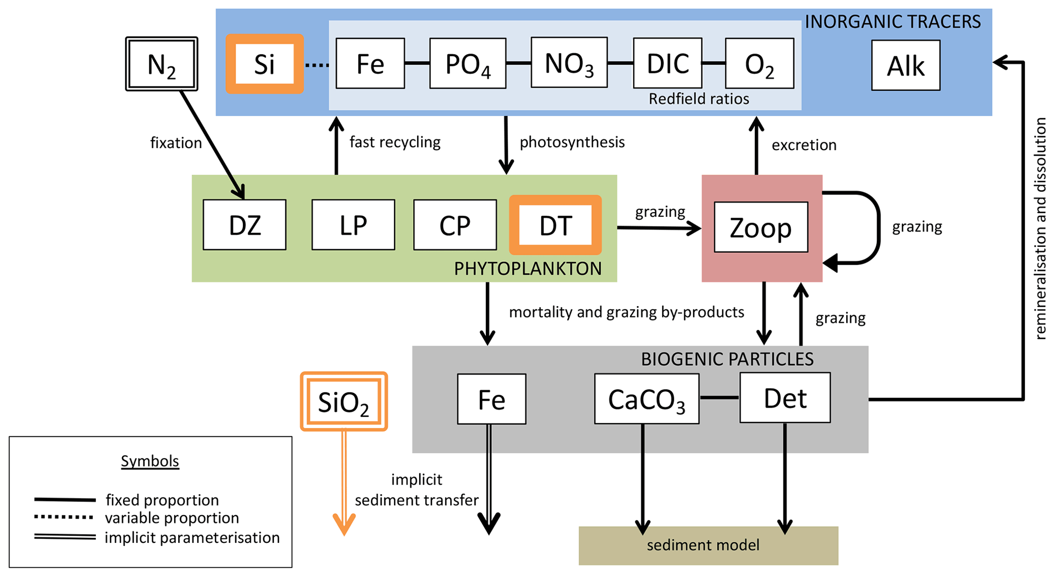
Figure 1The latest biogeochemical model structure for KMBM3. Previously unpublished features are shown in orange.
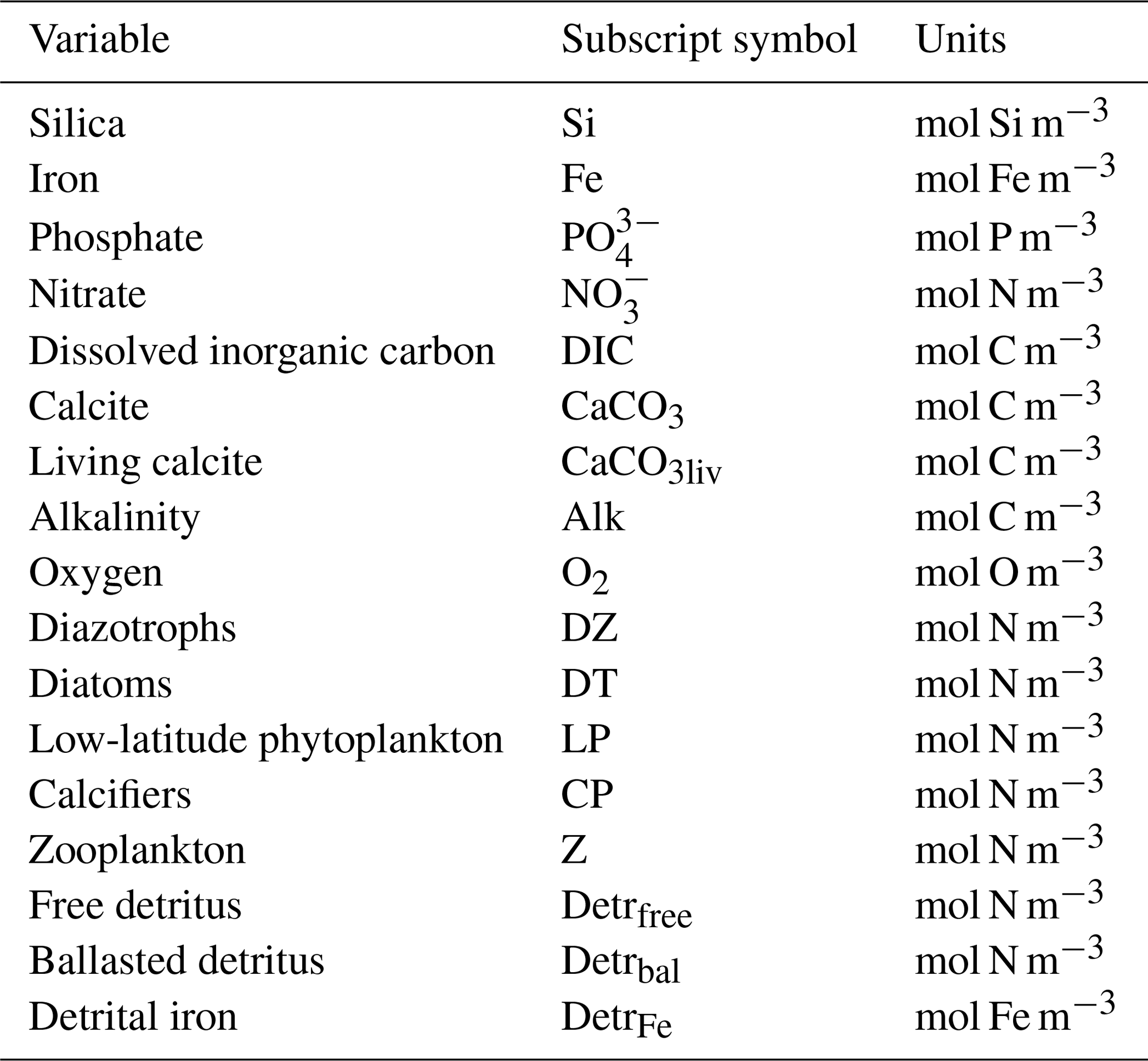
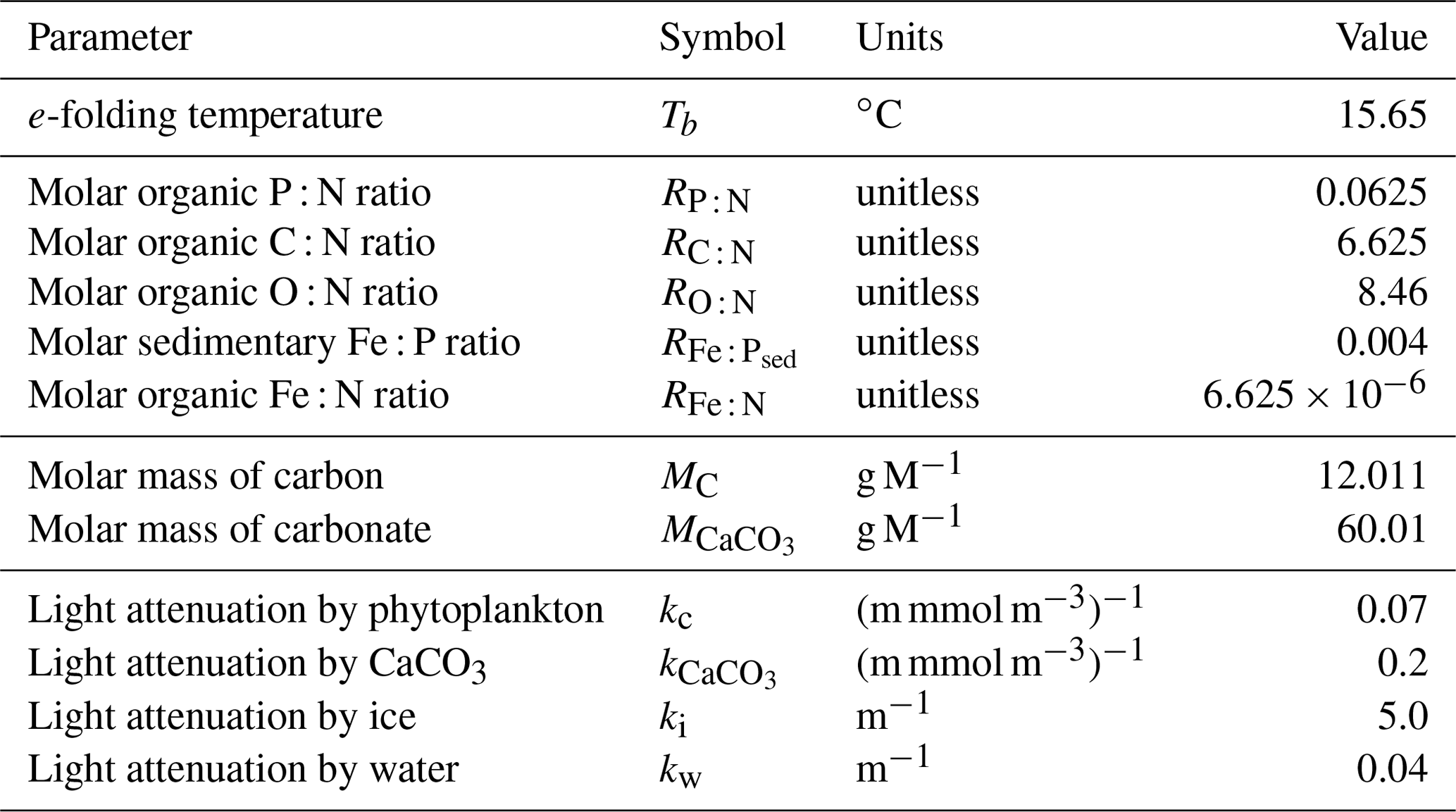
In the following model description, notation will generally follow the symbols used in Kvale et al. (2015b), with the abbreviations LP, CP, DT and DZ representing the phytoplankton functional types, and “Z” representing zooplankton when a distinction is necessary. The most important biogeochemical model parameters are listed in Tables 2 to 5. The model description here covers only the most relevant equations and equations that have changed in this newest version; please see Kvale et al. (2015b), Nickelsen et al. (2015), Keller et al. (2012) and Schmittner et al. (2005, 2008) for original references and a complete description of the other equations.
2.2.1 Sources and sinks
Tracer concentrations (C) vary according to
with T including all transport terms (advection, diffusion and convection), S representing all source and sink terms, and B representing air–sea interface boundary (including virtual evaporation–precipitation correction) fluxes and hydrothermal inputs, where relevant.
2.2.2 Phytoplankton
Phytoplankton (X representing all types except diazotrophs) biomass (in units of mmol nitrogen m−3) source and sink terms are
where growth (J), mortality (m) and fast recycling (μ*) rates are described below, and losses to zooplankton grazing (G) are described in the zooplankton equations. The diazotroph equation is similar except that it does not include a linear mortality loss, only a loss to fast recycling.
As in Keller et al. (2012), the maximum possible growth rate of phytoplankton (Jmax) is a modified Eppley curve (Eppley, 1972) and is a function of seawater temperature (T) in degrees Celsius, an e-folding temperature parameter Tb and iron limitation (uFe) modifying a growth parameter (a). This parameterization assumes sufficient iron is required for the utilization of other nutrients (Galbraith et al., 2010; Keller et al., 2012; Nickelsen et al., 2015).
As in earlier versions of the model, diazotroph growth rate is calculated following ordinary phytoplankton (now LP) and then multiplied with an additional handicap.
Nickelsen et al. (2015) assigned a constant iron half saturation (kFe) to diazotrophs, but in ordinary phytoplankton this parameter varied as a function of biomass (X) to implicitly represent different cell sizes in the model. Because KMBM3 contains multiple phytoplankton functional types, we revert to a prescribed but unique kFe for all functional types and calculate iron limitation as
The maximum potential growth rate is then multiplied by the minimum nutrient limitation term (u) for nitrate, phosphate and dissolved silicic acid (the latter for diatoms only) to calculate potential growth under nutrient limitation but replete light, where kN and kP are fixed half-saturation constants unique to each functional type (and kP is calculated from 16 P to 1 N Redfield stoichiometry). These equations are applied to obtain maximum possible growth rates as a function of temperature and nutrients following Liebig's law of the minimum:
Silica limitation uses the empirical fit to experimental data scaling of kSi in mmol Si m−3 from Aumont et al. (2003):
with a value adopted from Aumont et al. (2003) of 30 mmol Si m−3.
The potential growth rate under limited light availability (JI) but replete nutrients is calculated as
Nickelsen et al. (2015) introduced this parameterization to the model and discussed it at length; interested readers are recommended to read their Sect. 2.3.2. In the above equation, αchl is the initial slope of the photosynthesis versus irradiance (I) curve in chlorophyll units:
and θ is a Chl : C ratio (noting, chlorophyll is not a prognostic variable, Nickelsen et al., 2015):
The approximation of θ is simplistic and neglects other factors, e.g. irradiance, which can affect the ratio. For simplicity, the same maximum and minimum values of αchl and θ are used for all functional types.
Light attenuation by algae biomass and by coccoliths is included in the calculation of available irradiance at each depth level:
where PAR stands for the photosynthetically available radiation, kw, kc, and ki are the light attenuation coefficients for water, all phytoplankton, CaCO3 and ice, is the effective vertical coordinate, ai is the fractional sea ice cover, and hi and hs are calculated sea ice and snow cover thickness. Opal generated by diatoms is not explicitly traced and is therefore not included in the underwater light field.
The actual growth rate (JX) of phytoplankton is taken to be the minimum of the growth functions described above:
In Eq. (2), two loss terms other than predation are considered. Non-grazing mortality is parameterized using a linear mortality rate (m). Temperature-dependent fast remineralization is a loss term used to implicitly account for the microbial loop and dissolved organic matter cycling, and is parameterized using a temperature dependency multiplied by a constant () (Schmittner et al., 2008):
With this formulation, increasing seawater temperature increases the return of nutrients to the upper ocean.
2.2.3 Zooplankton
Changes in zooplankton population (Z) are calculated as the total ingested food (phytoplankton, zooplankton and organic detritus) scaled with a growth efficiency coefficient (ϖ) minus mortality. In addition to mortality from higher trophic level predation calculated with a quadratic mortality function (mZZ2), intra-guild predation is represented with a separate term (GZ) (Keller et al., 2012; Kvale et al., 2015b; Nickelsen et al., 2015).
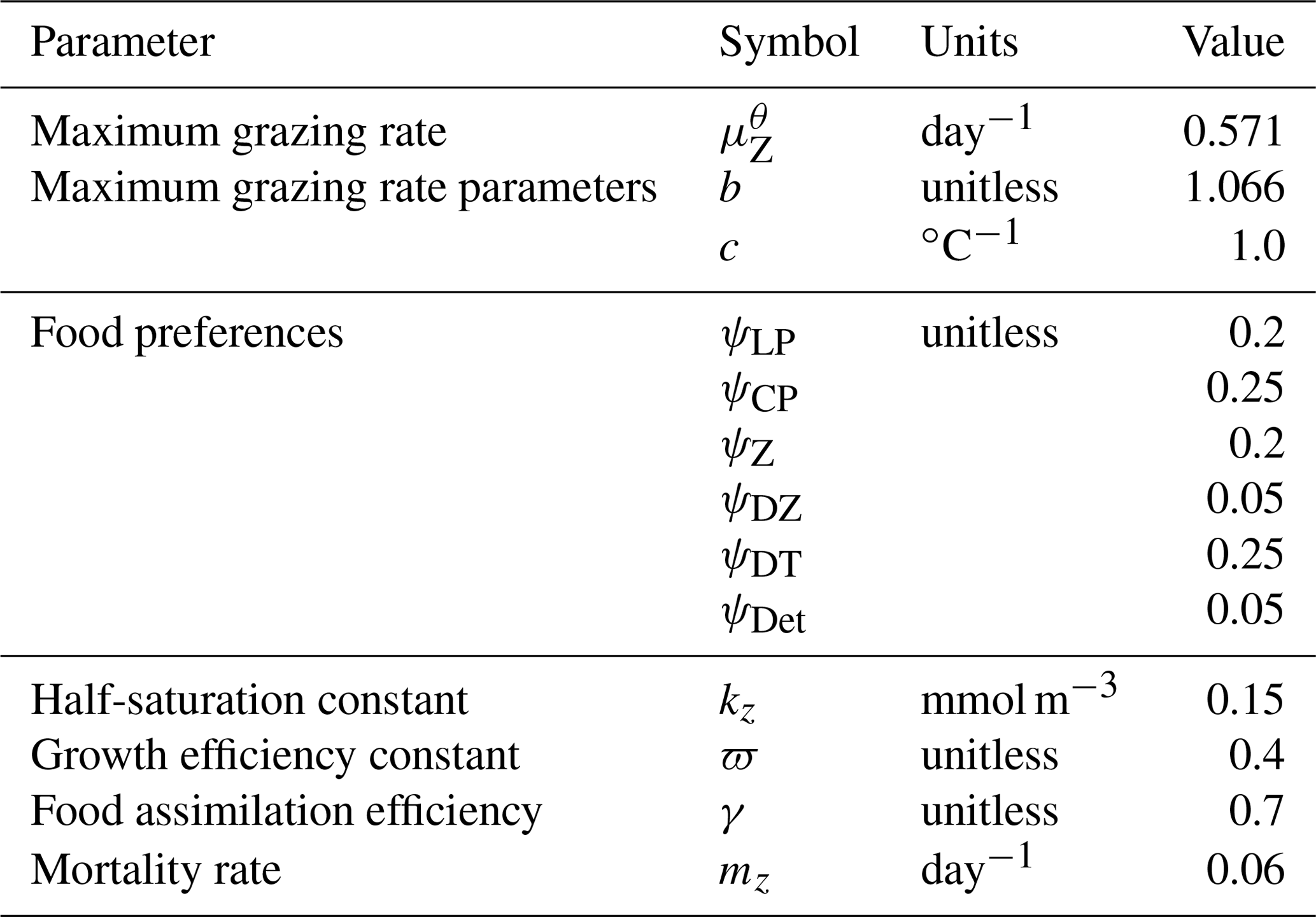
Zooplankton grazing (G) follows Keller et al. (2012). Relevant parameters are listed in Table 4. Grazing of each food source is calculated using a Holling II function, where a calculated maximum zooplankton grazing rate () is reduced by a scaling that is weighted by a relative food preference (ψX, where “X” stands for any of the food sources and the sum of all preferences must equal 1), the total prey population and a half-saturation constant for zooplankton ingestion (kz):
The calculated maximum potential grazing rate is a function of a maximum potential grazing rate at 0 ∘C (), temperature and oxygen, where grazing activity is capped when temperatures exceed 20 ∘C (Keller et al., 2012):
Grazing is also reduced under suboxic conditions ():
where O2 is dissolved oxygen in mmol m−3.
Table 3KMBM3 phytoplankton production and mortality parameters.
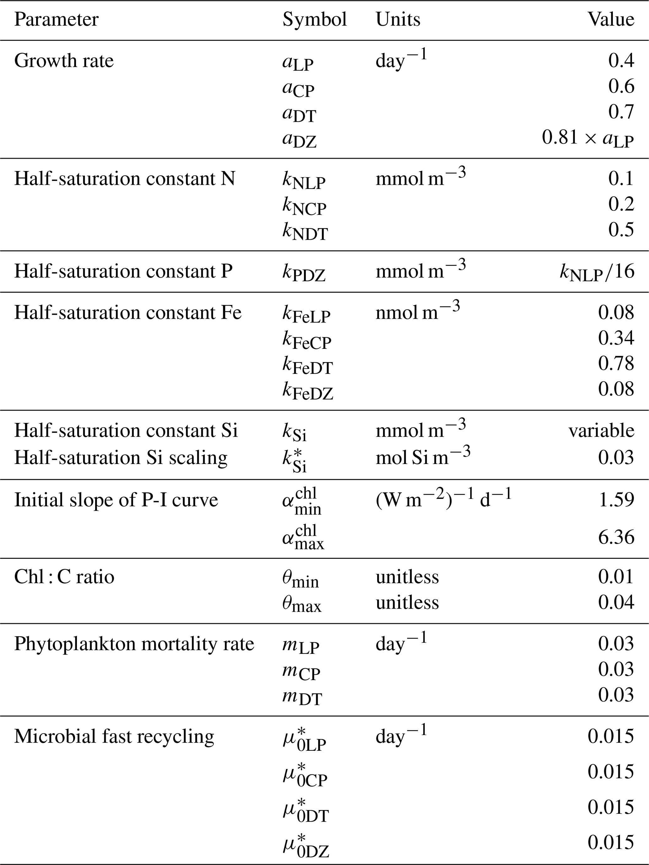
Table 4KMBM3 zooplankton parameters. Temperature-dependent parameter values are given for 0 ∘C.
2.2.4 Organic detritus
As was introduced in Kvale et al. (2015b), organic carbon detritus sources and sinks are split into “free” (Detrfree) and “ballast” (Detrbal) pools using a fixed ratio (Rbal : tot). Ballast detritus is formed from the CaCO3-protected portion of calcifying phytoplankton (CP) and zooplankton. This protected portion does not interact with nutrient pools directly and instead transfers from the “ballast” to the “free” detrital pool at the rate of CaCO3 dissolution ():
where γ is the food assimilation efficiency, is a fixed production ratio of CaCO3 to organic detritus, RC : N is a Redfield molar ratio, and wC is the sinking speed of calcite. Free detritus is described as
where μD is the detrital remineralization rate and wD is the sinking speed of organic detritus.
2.2.5 Detrital iron
Iron in detritus follows Nickelsen et al. (2015) but with the additional contribution of calcifiers and diatoms:
RFe : N is a fixed iron to nitrogen ratio that converts total organic nitrogen detritus sources into iron units. The remineralization and sinking of detrital iron occurs at the same rates as free organic detritus. Two scavenging processes are considered: adsorption of dissolved iron onto organic detritus ([Fe]orgads):
and particulate CaCO3 ():
calculated as a function of free organic detritus and carbonate particles converted to carbon units, respectively, a scavenging rate constant (kFeorg and kFeca), iron available for scavenging ([Fe′]) and inorganic precipitation of dissolved iron into colloidal material ([Fe]col), which is calculated as a linear function independent of organic particle concentration and unchanged from Nickelsen et al. (2015). While calcite is known to be a powerful scavenger of iron and other trace metals (Olsson et al., 2014), the strength of plankton-derived calcite in scavenging dissolved iron is unquantified. A test of this sensitivity is planned at a later stage, so for now the calcite scavenging parameter value is set equal to that of organic detritus.
2.2.6 Calcite
As in Kvale et al. (2015b), the source and sink terms for CaCO3 include both phytoplankton calcifier and zooplankton sources from grazing and mortality, and losses from dissolution and sinking:
where wC is the sinking speed of calcite, and the dissolution-specific rate () is calculated using a parameterization from Aumont et al. (2003) and Kvale et al. (2015b).
Calcite associated with living plankton is calculated separately (but not traced) as
2.2.7 Opal
The production of biogenic opal is calculated as a function of the diatom grazing and linear mortality loss terms:
where ROpal : POC is a production ratio that varies as
This parameterization was introduced by Aumont et al. (2003) and yields an average surface opal : free detritus export value of around 1 Si : C across the Southern Ocean, using a fixed average ratio (R) of 0.5. Production of lithogenic opal occurs mostly on land (Tréguer and De La Rocha, 2013), so its contribution to marine silicate cycling is included simplistically via the dissolved silicate river flux calculation. In linking opal production to diatom mortality, our model essentially focuses on the importance of its export pathway in establishing vertical gradients. Opal that is not exported is effectively assumed to be recycled to dissolved silicate within the surface layer.
Dissolution of opal in the water column is calculated by assuming instantaneous sinking of the vertically integrated production, where the local flux of opal (FOpal in mol Si m−2) is distributed down the water column using the e-folding temperature parameterization (unitless), scaled by a dissolution rate constant (λOpal, in day−1), which is divided by a sinking rate (wOpal, in metres day−1):
Dissolution is presented in units of mol Si m−3 d−1. This parameterization results in greater dissolution at warm temperatures and is similar to the instant-sinking-and-dissolution function applied to model calcite (Schmittner et al., 2008). Opal dissolution in the water column is primarily controlled by temperature and silicate saturation, with higher temperatures and lower silicate saturations leading to faster dissolution (Sarmiento and Gruber, 2006; Ridgwell et al., 2002). Secondary drivers include the aluminium content and surface area of diatom shells (Van Cappellen et al., 2002), and the presence or absence of organic coatings, where the loss of the coating increases opal dissolution rates (Bidle and Azam, 1999). We do not consider silicate or aluminium concentration dependencies explicitly in this model because we do not explicitly calculate thermodynamic dissolution of opal (nor do we simulate aluminium), but the temperature dependency exerts an influence on dissolution of the same sign (faster dissolution in warmer, i.e. shallower and undersaturated, water). We find this parameterization offers improved model fit to World Ocean Atlas silica distributions relative to other parameterizations that we tested, e.g. the temperature-dependent parameterization of Gnanadesikan (1999) or the temperature- and oxygen-dependent parameterization of Enright et al. (2014). The Gnanadesikan (1999) parameterization yields lower dissolution rates at low temperatures than the Enright et al. (2014) parameterization, which is similarly formulated but includes additional oxygen scaling. The Enright et al. (2014) oxygen scaling is not justified in their model description, but it has the effect of increasing Si dissolution rates in the deep ocean (exacerbating the over-estimation of Si dissolution in this region by the Gnanadesikan, 1999 scaling described in Ridgwell et al., 2002) and decreasing Si dissolution rates (to a lesser extent) in the near-surface area. Our temperature scaling has the effect of raising dissolution rates at the surface. Greater dissolution rates at the surface may be necessary to compensate for the low vertical resolution of the model. Global average implicit opal export, dissolution and seafloor loss rate profiles are plotted in Fig. 2 for model year 2014. Consistent with the estimates of Tréguer et al. (2021), opal cycling in the open ocean largely occurs in the shallower depths, with opal export following a power law decrease with increasing depth. The global ocean average opal dissolution rate at 1000 m depth is only half that at the ocean surface, and the average flux of opal at the seafloor at 500 m depth is only half that at the surface. Shallow shelf areas are hence an important and relatively fast region of turnover for our simulated silicate cycle.
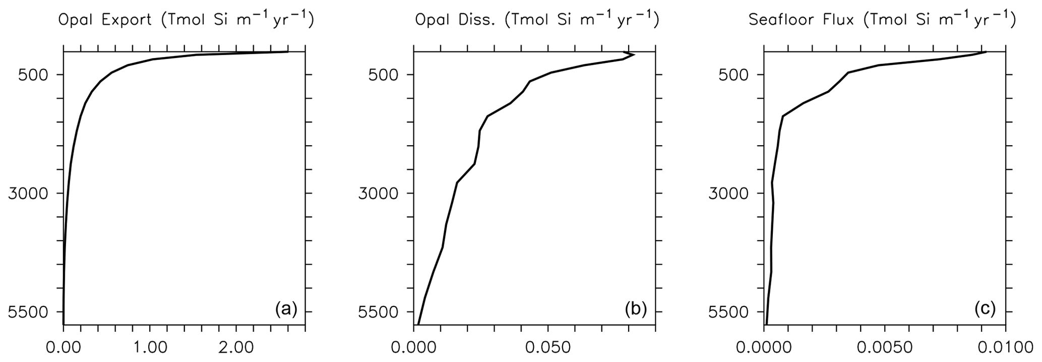
Figure 2Implicit opal export (a), water column dissolution (b) and seafloor burial (c) at model year 2014. Rates are globally integrated in the latitudinal and longitudinal planes but depth information is retained. Thus, opal export, dissolution and seafloor flux are reported in Tmol Si flux per metre of depth per year.
2.2.8 Particle sinking
Detritus (Schmittner et al., 2005), calcite (Kvale et al., 2015b) and iron (Nickelsen et al., 2015) particles are exported from the surface with a sinking speed (w) that increases linearly (wdc, wdd) with depth (z; Berelson, 2001) for calcite and ballasted organic detritus:
and free detritus and associated iron:
Alternative parameterizations exist and their effects on fluxes and model performance make for interesting comparisons (e.g. Kriest and Oschlies, 2011; Cael and Bisson, 2018), but we do not explore them here. The initial surface sinking speeds of particles are assigned different values to represent the denser structure of CaCO3 relative to that of organic detritus. Ballasted detritus sinks at the CaCO3 speed, but once it enters the free pool it uses the organic detrital sinking speed and remineralization rate. Any organic detritus reaching the sediments is dissolved back in to the water column to ensure conservation of carbon and phosphate in the model domain. Calcite particles that reach the seafloor enter the sediment model (Kvale et al., 2015b) if it is active, though we do not use it here (in this case, the particles dissolve instantly at the seafloor). Iron detritus reaching the sediments is lost from the ocean, unless bottom water oxygen falls below 5 mmol m−3, whereupon detrital iron reaching the bottom is dissolved back into the water column (Nickelsen et al., 2015). By definition, iron is not mass conserving in the model, but is formulated with open boundary conditions (atmosphere and sediments); hence, it is not just the oxygen threshold that can cause a loss or gain of marine iron. In the model, the oxygen threshold is only met along coastal boundaries in the North Pacific under modern conditions. A sedimentary release of dissolved iron ([Fe]sed) is prescribed as in Nickelsen et al. (2015):
where is a ratio of iron released from sediment in proportion to the flux of phosphorus in the organic detritus (FPOP, which includes free and ballast detritus) reaching the bottom.
Opal reaching the seafloor is either returned to the silicic acid tracer or considered lost to the sediments ([Si]sed) according to criteria laid out in Sarmiento and Gruber (2006):
Opal flux, F(Opal), is calculated as depth-integrated opal production (Pr(Opal)) less the depth-integrated instantaneous dissolution term (Di(Opal)). The model conserves silica when river fluxes are allowed to compensate for the net change due to the ocean sedimentary sink, hydrothermal input and atmospheric deposition.
The subgrid bathymetric scaling that was introduced for the iron model in Nickelsen et al. (2015) is extended here to apply to all particle fluxes reaching the bottom ocean grid. This scaling feature calculates a sedimentary exchange factor based on the proportion of each grid cell that falls outside of the model grid's depth according to a high-resolution bathymetric dataset. This scaling is used to account for high-relief bathymetric features, such as ridges and troughs, in the sediment transfer functions. We do not use the sediment model in this paper.
2.2.9 Dissolved inorganic tracers
Ocean nutrient sources and sinks (in concentration/time units) follow
where RP : N and RO : N are Redfield molar ratios and is nitrate availability (diazotrophs use nitrate when available). In suboxic water (less than 5 mmol m−3), oxygen consumption is replaced by denitrification ():
There are no additions of phosphate, nitrate or oxygen along the boundary (with the exception of air/sea gas exchange in the case of oxygen; Keller et al., 2012).
Dissolved iron includes sources and sinks of particulate iron mentioned above, as well as prescribed dust deposition ([Fe]dust) as in Nickelsen et al. (2015) and hydrothermal iron ([Fe]hydr) (Muglia et al., 2017) boundary terms (also in concentration/time units):
The Nickelsen et al. (2015) model applied the iron dust flux to the surface ocean after the biological routine and before the mixing routine. This resulted in low model sensitivity to iron dust inputs, because the dust was mixed away faster than the biological processes had a chance to access it. In this version, the iron dust flux is added prior to the biological routine (which operates on a shorter time step than ocean mixing) and results in a greater biological sensitivity to iron dust flux.
DIC and alkalinity tracer sources and sinks are a function of sources and sinks of prognostic CaCO3 (Kvale et al., 2015b).
With the exception of air–sea gas exchange of CO2, there are no boundary additions of DIC or alkalinity when the sediment model is deactivated (as is presented here).
Dissolved silicic acid tracer sources, sinks and boundary terms (all in concentration/time units) follow
where discharge from rivers ([Si]riv) is used as a budget balancing term to compensate for any remainder in the other external sources and sinks: wind-borne dust ([Si]dust), hydrothermal silicate ([Si]hydr) and loss to the sediments ([Si]sed). River inputs of silicate, alkalinity and DIC are scaled against seasonally variable river flow using the standard UVic ESCM version 2.9 O_rivflux.F forcing file. Dust deposition from the atmosphere is prescribed using an interpolated monthly pre-industrial dust flux derived from the NCAR's Community Climate System Model (Mahowald et al., 2006). The silica content of the dust is derived from maps (Zhang et al., 2015), with a global average dust solubility of 3 % assumed to produce annual bioavailable fluxes in agreement with estimates (Sarmiento and Gruber, 2006; Tréguer and De La Rocha, 2013). Observations demonstrate wide spatial variability in the solubility parameter (Tréguer and De La Rocha, 2013), so our single value represents a simplification. Silicate from hydrothermal sources are prescribed using a static mask scaled from the hydrothermal iron mask (Muglia et al., 2017) using a Fe : Si ratio to obtain the estimated annual total contribution from hydrothermal sources in Sarmiento and Gruber (2006) (0.6 Tmol Si yr−1). This estimate has recently been revised upward to 1.7 ± 0.8 Tmol Si yr−1 (Tréguer et al., 2021); thus, our hydrothermal contribution is under-estimated. Model sensitivity to both sources will be explored in future tests.
The model is spun up to equilibrium (greater than 15 000 years) at year 1765 boundary conditions, then forced with historical data for comparison to observational datasets. Forcing includes historical atmospheric CO2 concentrations, agricultural land cover, volcanic radiative forcing, sulfate aerosol and chlorofluorocarbon (CFC) concentrations, changes in land ice and solar forcing (Machida et al., 1995; Battle et al., 1996; Etheridge et al., 1996, 1998; Flückiger et al., 1999, 2004; Ferretti et al., 2005; Meure et al., 2006). Solar insolation at the top of the atmosphere, wind stress and wind fields vary seasonally (Kalnay et al., 1996), and wind fields are geostrophically adjusted to air temperature anomalies (Weaver et al., 2001).
Table 6 lists key biogeochemical properties diagnosed by the model for a modern climate, as well as corresponding properties diagnosed from KMBM1 (Keller et al., 2012). We compare model output at the year 2004, although data sources reflect a range of collection and publication dates. Net primary production (NPP) is similar to previous model versions (53.60 Pg C yr−1, e.g. compared to 54.33 Pg C yr−1 in Keller et al., 2012), and still within the literature range of 44–78 Pg C yr−1 (e.g. Carr et al., 2006; Jin et al., 2006). Calcite production is similar to and nitrogen fixation rates are somewhat improved with respect to earlier model versions, though they remain too low, as do deep particle fluxes of particulate organic carbon (POC) and shallow and deep calcite (also referred to as PIC, for particulate inorganic carbon). Diagnosed surface opal production is also too low and below the range of a recent estimate (Tréguer et al., 2021). Accordingly, deep ocean (2 km depth) opal fluxes are also too low (only about 50 % of the observationally based deep ocean estimates of Tréguer and De La Rocha, 2013). However, upper ocean (130 m) opal flux is about 9 % larger than the estimate provided by Tréguer et al., 2021. This may be due to the model under-estimating upper-ocean dissolution (10.3 Tmol Si yr−1 in our model compared to 124 Tmol Si yr−1 estimated in the surface mixed layer by Tréguer et al., 2021). There is too little dissolution of opal throughout the water column (74 % of the observational estimate in Tréguer et al., 2021, but the ratio of total water column dissolution to biogenic production is too high, with a ratio of 0.95 compared to 0.67 calculated by Tréguer et al., 2021). The calculated river flux is 2.38 Tmol Si yr−1; this is lower than the Tréguer et al. (2021) estimate of 8.1 Tmol Si yr−1. Overall, an increase in production and subsequent processes is required to improve the model agreement with independently estimated fluxes. Low bias in fluxes is also found in calcite production and nitrogen fixation, as well as in deep particle fluxes, which is due at least in part to the model bias of a too-sluggish deep circulation (Kriest et al., 2020). The calculated flux of silicate through the seafloor is only 70 % of that estimated by Tréguer et al. (2021). An under-estimation of seafloor flux is potentially corrected with an increase in pelagic opal production rates or an decrease in benthic return. Benthic fluxes are potentially improved with newer models of benthic transfer (e.g. Dale et al., 2021) and will be explored in the future. A recent review suggests the global silicate cycle sources and sinks are roughly balanced, but uncertainties are still substantial (Tréguer et al., 2021). It should be noted that the global silica cycle may be unbalanced between sources and sinks at present and observations of global input and output rates are both affected by anthropogenic perturbation and have large uncertainties (Tréguer and De La Rocha, 2013). Atmospheric and hydrothermal silica inputs are fixed in these simulations, but each source and sink of silicate produce a unique spatial distribution in the water column. These terms are slated for automated calibration in the future (e.g. Yao et al., 2019; Kriest, 2017; Kriest et al., 2017); thus, our hand-tuned simulations are meant to serve as a baseline for future improvements to the model. Also note that despite the deficiencies described above, KMBM3 demonstrates reasonable performance against a suite of state-of-the-art Earth system models (described below).
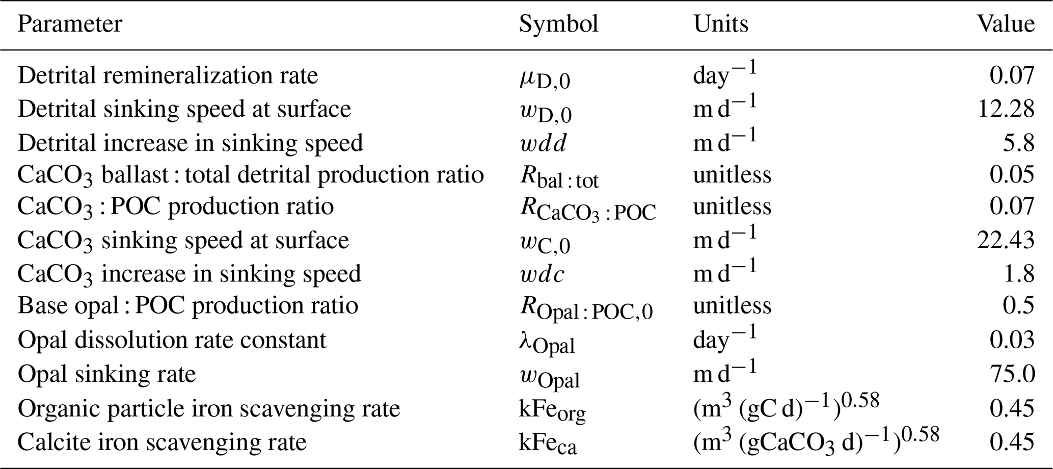
Table 6Globally integrated diagnosed biogeochemical properties at the year 2004. Corresponding values are also given using KMBM1 (Keller et al., 2012).

a Carr et al. (2006), Jin et al. (2006). b Smith and Gattuso (2011), Smith and Mackenzie (2016). c Tréguer et al. (2021). d Luo et al. (2014). e All particle fluxes from Honjo et al. (2008) unless noted. f Luo et al. (2014). g All biomass estimates from Buitenhuis et al. (2013). h Picophytoplankton. i Pteropods.
Total global phytoplankton biomass is on the low end, but within the range, of previous estimates (0.55 Pg C, virtually unchanged from Keller et al., 2012, compared to 0.5–2.4 Pg C from Buitenhuis et al., 2013; Table 6). KMBM3 explicitly represents only a fraction of the ecological complexity found in the real ocean, which causes our biomass estimates for the phytoplankton functional types to look dissimilar to the Buitenhuis et al. (2013) biomass estimates (e.g. with low-latitude mixed phytoplankton (a model-specific category, LP) having a biomass only 11 % of the lowest picophytoplankton estimate and both diazotrophs (DZ) and calcifiers (CP) having more biomass than the upper observational estimate). These functional types proved particularly difficult to tune by hand, with small variations in parameter values causing extinction. An over-estimate of calcifiers is compensated by the low PIC : POC production ratio (0.07), which is meant to represent 7 % of the phytoplankton class having a PIC : POC production ratio of 1 (compare to a ratio for Emiliania huxleyi of 0.51–2.30 from Paasche, 2001). Over-estimated diazotroph biomass results in an increase (0.04 Pg N yr−1) in nitrogen fixation compared to earlier model versions, which is improved with respect to, but still lower than, the observational independent estimate. In KMBM3, diazotrophs use preformed nitrate when available. Thus in our modelling context, this functional type can be considered “slow-growing phytoplankton capable of fixing nitrogen when necessary”. Constraints on this functional type will be explored in the future. Diatom biomass estimates are too low and outside the Buitenhuis et al. (2013) range, although the functional type is represented in the same relative proportion to low-latitude phytoplankton (LP) as is reported for picophytoplankton to diatoms by Buitenhuis et al. (2013).
Looking next at spatial distributions of biological rates, Fig. 3 compares KMBM3 NPP at year 2014 to the Westberry et al. (2008) model applied to MODIS (NASA, 2018) climatology from 2012–2018. As is repeatedly found in KMBM (see plot of the Keller et al., 2012 model NPP), open-ocean primary production rates are generally too high, particularly in the eastern equatorial Pacific and northern Indian Ocean. These very-high-production zones compensate in the globally integrated rate estimate for the diffuse and more widespread production calculated from satellites. The spatial pattern in NPP has changed somewhat from earlier model versions, with a continued under-estimate of NPP occurring within gyres and a new over-estimate of NPP in the 40–60∘ N and S ranges.
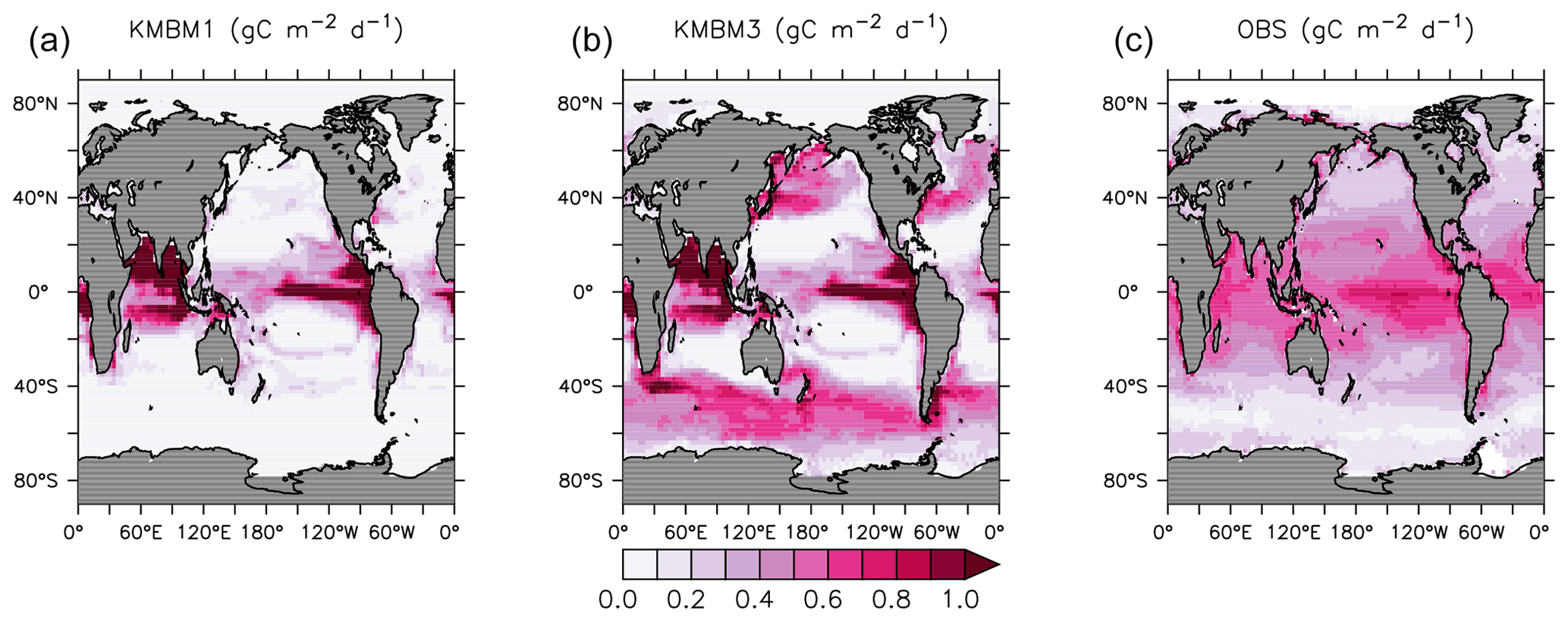
Figure 3Comparison of model NPP output at 2014 (a Keller et al., 2012; b this model) and satellite-derived NPP climatology (NASA, 2018), 2012–2018 (c) in gC m−2 d−1.
Spatial biases in NPP are also held in surface calcite concentrations. Figure 4 compares KMBM3 CaCO3 averaged between 2004–2014 with the 2002–2018 climatology data from MODIS (NASA, 2018). Model calcite is too high in the North Pacific and Southern Ocean between 40 and 60∘ S, and too low south of 60∘ S. Upwelling zones and the Indian Ocean have an over-estimated role in calcite production, and coastal calcite production is either not resolved or under-estimated.

Figure 4Comparison of model average 2004–2014 (a) and satellite CaCO3 climatology 2002–2018 (b) in mmol CaCO3 m−3. Data product is scaled by the model grid in the z direction, and in both plots only the upper 20 m are represented, where uniform coccolith concentration is assumed (Balch and Utgoff, 2009).
Phytoplankton biomass is compared to the MARine Ecosystem DATa (MAREDAT) datasets (Leblanc et al., 2012; Luo et al., 2012; O'Brien, 2012) in Fig. 5. Globally integrated diatom biomass is too low compared to observational estimates but the diatom geographical distributions agree roughly with the very sparse Leblanc et al. (2012) dataset (highest concentrations in the Southern Ocean, North Pacific and North Atlantic). Like the globally integrated biomass estimate, calcifiers (CP) are universally over-estimated compared to O'Brien (2012). As explained above, this functional type is meant to represent a variety of moderate growth, moderate nutrient affinity phytoplankton types, including those that calcify. Therefore, it is not unexpected to have an over-estimate of the biomass. Diazotroph biomass is primarily concentrated in the tropics, which agrees spatially but not in magnitude with the limited data of Luo et al. (2012). Mixed low-latitude phytoplankton (LP) is a model-specific category with no clear analogue in the MAREDAT dataset.
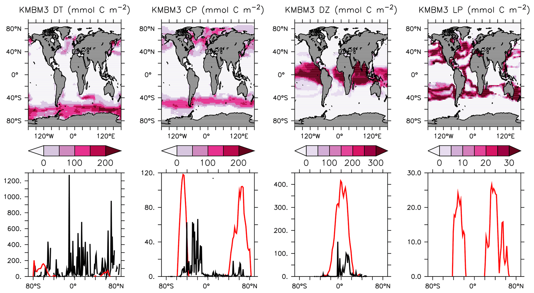
Figure 5Annually averaged and depth-integrated model biomass at the year 2014 (top row). Zonally averaged and depth-integrated model biomass plotted with the equivalent MAREDAT compilations (bottom row; Leblanc et al., 2012; O'Brien, 2012; Luo et al., 2012; no data compilation of “mixed” phytoplankton, a model-specific category). All units are mmol C m−2. Black lines represent MAREDAT; red lines are the model output.
We compare CMIP6 model output relative to KMBM3 model output due to the very low normalized correlation (0.04–0.15) and normalized standard deviation (0.10–0.22) of all models against the sparse Leblanc et al. (2012) diatom biomass dataset. At the time of writing, available CMIP6-simulated annual average diatom biomass shows diverse quantities (maximum concentrations from 0.0035 to 0.03 mol C m−3) and spatial distributions ranging from global maximum concentrations at the Equator (CanESM5-CanOE, Swart et al., 2019), to shallow seas and coastlines (IPSL-CM6A-LR, Boucher et al., 2018), to the high latitudes (CMCC-ESM2, EC-Earth3-CC, GFDL-ESM4, CESM2; Lovato et al., 2021; EC-Earth Consortium, 2021; Krasting et al., 2018; Danabasoglu, 2019, respectively). Figure 6 contextualizes these diatom biomass estimates relative to the KMBM3 diatom biomass, simulated at year 2014. KMBM3 is most closely correlated with GFDL-ESM4. KMBM3 has a near-perfect standard deviation and second-closest correlation with CMCC-ESM2, a higher-resolution fully coupled Earth system model with full representation of the global carbon cycle and ocean biogeochemistry. The CMCC-ESM4, KMBM3, CESM2 and CanESM5-CanOE models all fall outside the cluster in correlation and standard deviation of EC-Earth3-CC, IPSL-CM6A-LR and GFDL-ESM4. EC-Earth3-CC and IPSL-CM6A-LR both utilize the PISCES biogeochemical model (and are therefore expected to show similar correlation and standard deviation relative to a reference model), but GFDL-ESM4 utilizes COBALT (an independent biogeochemical model lineage). As stated above, phytoplankton biomass is difficult to tune for (particularly when multiple functional types are represented) due to the under-constrained parameter space, the theoretical nature of phytoplankton functional categories and the sparsity of gridded, annually averaged biomass datasets. Therefore, a wide range in model biomass estimates is expected across the CMIP6 ensemble.
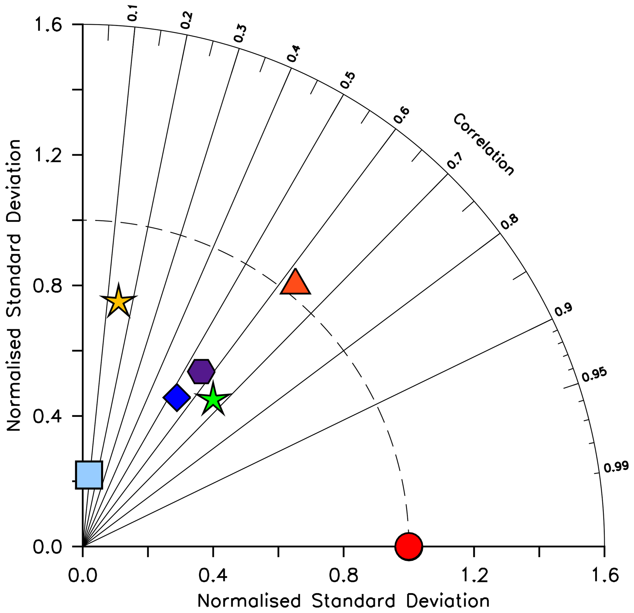
Figure 6Taylor diagram (Taylor, 2001) of CMIP6 annual average diatom biomass concentrations (in mol C m−3) at the year 2014 referenced to KMBM3. The distance to the origin represents the normalized standard deviation. Normalized correlation with KMBM3 is read from the azimuthal position. Perfect agreement with KMBM3 is a normalized standard deviation of 1 and a normalized correlation of 1. Normalization against the model, rather than observations, is shown due to the models having greater similarity with each other than with the very sparse observations of diatom biomass currently available. Models are KMBM3 (red circle), GFDL-ESM4 (green star; Krasting et al., 2018), CanESM5-CanOE (yellow star; Swart et al., 2019), CESM2 (light blue square; Danabasoglu, 2019), CMCC-ESM2 (orange triangle; Lovato et al., 2021), EC-Earth3-CC (blue diamond; EC-Earth Consortium, 2021) and IPSL-CM6A-LR (purple hexagon; Boucher et al., 2018). With the exception of KMBM3, the data for all models were obtained by mining the CMIP6 database (https://esgf-node.llnl.gov/search/cmip6/, last access: 5 February 2021) using the following search terms: CMIP/phydiat/historical/annual output. Data were accessed between 1–5 February 2021.
KMBM3 interior ocean particle flux performance is encouraging. Figure 7 compares model POC, PIC and opal fluxes at 2 km depth to the Honjo et al. (2008) data compilation. The model shows a general under-estimate with respect to the observations for all deep ocean particle fluxes, particularly for intermediate rates. Root mean square error is improved beyond Kvale et al. (2015a) for PIC (101.4 compared to 147.1 mmol C m−2 yr−1) and POC (96.7 versus 98.0 mmol C m−2 yr−1 in Kvale et al., 2015a). Root mean square error for opal flux at 2 km depth is 223.0 mmol Si m−2 yr−1. However, the model captures large-scale features of high flux rates in the north west Pacific and Southern Ocean, as well as moderate flux rates in the Indian and North Atlantic basins. KMBM3 demonstrates moderate skill at simulating annual average deep ocean opal fluxes relative to CMIP6 models (Fig. 8), with two of six models having a lower correlation with the Honjo et al. (2008) data compared to KMBM3 and four of six having a lower, or equal, normalized standard deviation. Two of six have an over-estimated bias in opal flux, relative to KMBM3. The GFDL-ESM4 performs best against the Honjo et al. (2008) dataset of the model simulations examined here.

Figure 7Comparison of model POC (a, d), CaCO3 (b, e) and opal (c, f) fluxes at the year 2004 and 2 km depth with Honjo et al. (2008) data. Red points are this model (KMBM3); blue points are the Keller et al. (2012) model (KMBM1). Statistics are given for KMBM3 only.
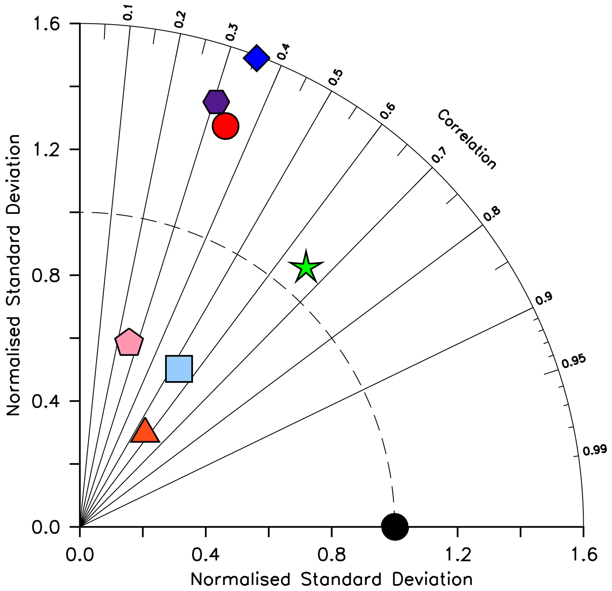
Figure 8Taylor diagram (Taylor, 2001) of CMIP6 annual average opal flux (in mol Si m−2 yr−2) at 2 km depth, for the year 2014, normalized to the Honjo et al. (2008) dataset. The distance to the origin represents the normalized standard deviation. Normalized correlation with observations is read from the azimuthal position. Perfect agreement with observations is a normalized standard deviation of 1 and a normalized correlation of 1. Models are KMBM3 (red circle), GFDL-ESM4 (green star; Krasting et al., 2018), CESM2 (light blue square; Danabasoglu, 2019), MPI-ESM1.2-LR (pink pentagon; Wieners et al., 2019), CMCC-ESM2 (orange triangle; Lovato et al., 2021), EC-Earth3-CC (blue diamond; EC-Earth Consortium, 2021) and IPSL-CM6A-LR (purple hexagon; Boucher et al., 2018). With the exception of KMBM3, the data for all models were obtained by mining the CMIP6 database (https://esgf-node.llnl.gov/search/cmip6/) using the following search terms: CMIP/expsi/historical/annual output. Data were accessed between 1–5 February 2021.
Particle flux rates, alongside the model's ocean circulation, impact ocean tracer distributions. Figure 9 shows carbon and nutrient profiles, globally averaged and for each basin, compared to Global Ocean Data Analysis Project (GLODAP) (Key et al., 2015; Lauvset et al., 2016) and World Ocean Atlas (WOA) (Garcia et al., 2014a, b) data. Nutrients are generally too high at depth, and oxygen is too low, partly as a result of over-estimated deep ocean POC flux rates in the Southern Ocean. Global root mean squared error is listed in the figure for each model dissolved inorganic tracer. All tracers except DIC, phosphate and oxygen show improvement with respect to the Keller et al. (2012) model version. Alkalinity is primarily affected by PIC flux and attenuation rates and shows relatively good agreement (global RMSE value of 0.34 µmol kg−1) with observations. Silicic acid has a global root mean squared error of 0.388 mmol Si m−3. Concentrations are too high in the Atlantic by as much as 50 mmol Si m−3 and too low in the Indian Ocean by as much as 50 mmol Si m−3.
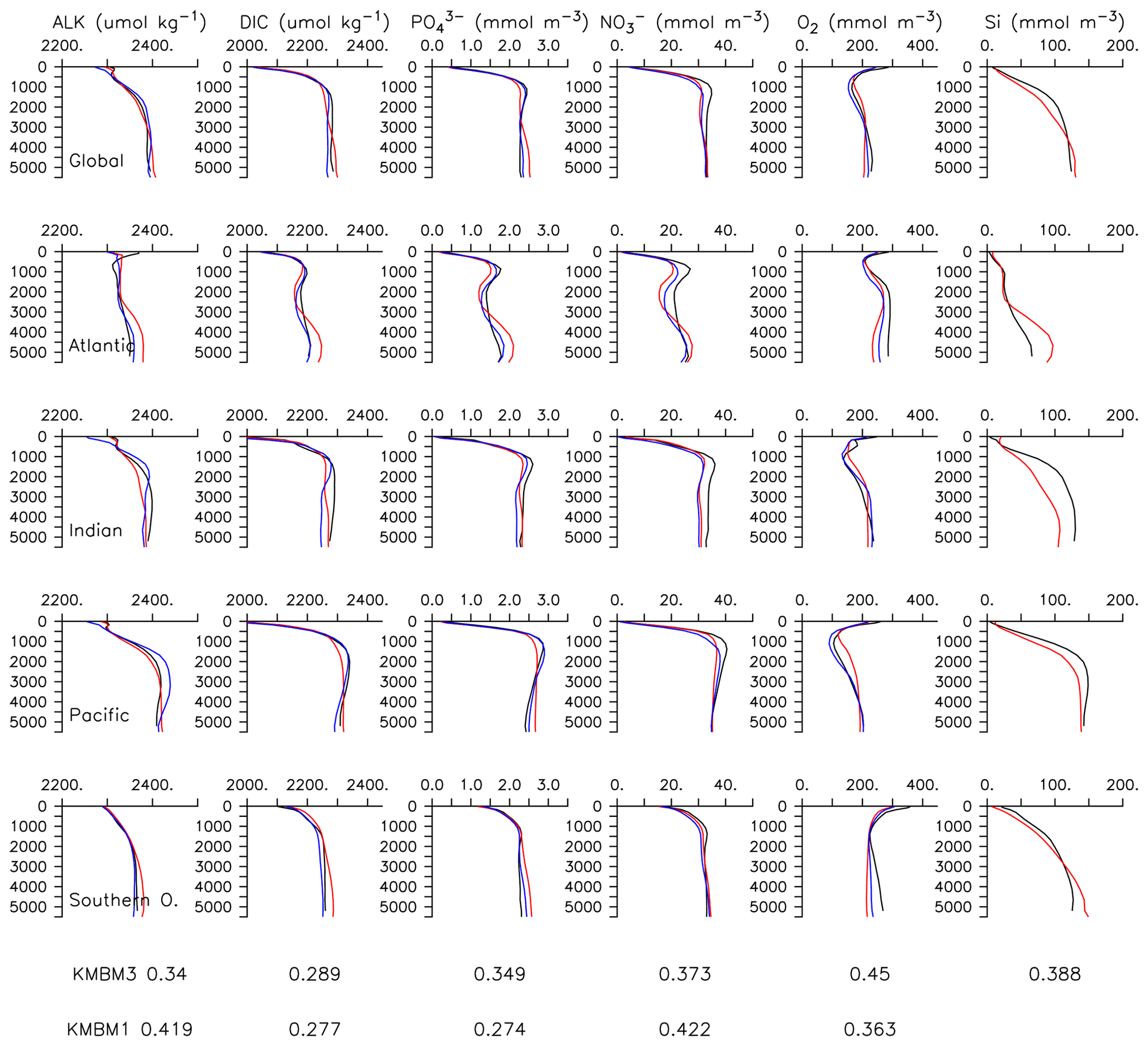
Figure 9Model global and basin average nutrient and carbon depth profiles at the year 2014 (KMBM3; red lines), compared to model output from the Keller et al. (2012) version (KMBM1; blue lines) and observational data (black lines; Garcia et al., 2014a, b; Key et al., 2015; Lauvset et al., 2016). Global root mean square error is given below each column.
Greater basin and surface detail in carbon and nutrient concentrations is displayed in Figs. 10–15. Interior ocean alkalinity is too high by as much as 50 µmol kg−1 and surface alkalinity too low by as much as 50 µmol kg−1, in the Atlantic, as it was with previous model versions (Eby et al., 2009; Keller et al., 2012; Kvale et al., 2015a). Alkalinity in the interior and surface Pacific is too high by as much as 20 µmol kg−1 along the Equator, whereas previously it was over-estimated at depth and under-estimated at the surface (Kvale et al., 2015a). The physical circulation has not changed since previously published model versions. Differences might be partly due to shifts in phytoplankton biogeography and calcification rates. Note, however, that surface alkalinity is also subject to evaporation–precipitation effects that might have also changed since previous model versions. The Indian Ocean interior alkalinity is under-estimated by as much as 60 µmol kg−1. Deep ocean DIC is not improved with respect to past model versions (Fig. 11), though (at least compared to Kvale et al., 2015a) this discrepancy might be partly attributed to the use of a transient year 2014 model output that includes an anthropogenic signal, instead of the pre-industrial spinup. The deep North Pacific shows a low bias of up to 40 µmol kg−1, similar to previous versions. Surface DIC anomalies are also similar to previous model versions, with DIC being too low in the western Pacific (a consequence of too-high export production in the model and physical biases) and too high in the surface Southern Ocean. As with earlier model versions, deep ocean phosphate concentrations (Fig. 12) are also generally too high, particularly in the Southern Ocean-sourced deep and intermediate water masses in the Indian and Pacific sectors. Nitrate, however, is too low in these water masses (Fig. 13), although in basin average the depth profiles of KMBM1 and KMBM3 are nearly identical for the Southern Ocean, Pacific and Indian basins below 3000 m. Oxygen anomalies mirror nutrient biases (Fig. 14), with oxygen being up to 50 mmol m−3 too low along the Southern Ocean particle export pathway and up to 50 mmol m−3 too high in the subsurface tropical ocean. The oxygen bias in the deep water masses might be addressed with better tuning of the biological production, export and flux parameters, but the tropical ocean deficiencies will require improvements to both the biogeochemistry as well as the physics (Oschlies et al., 2017).
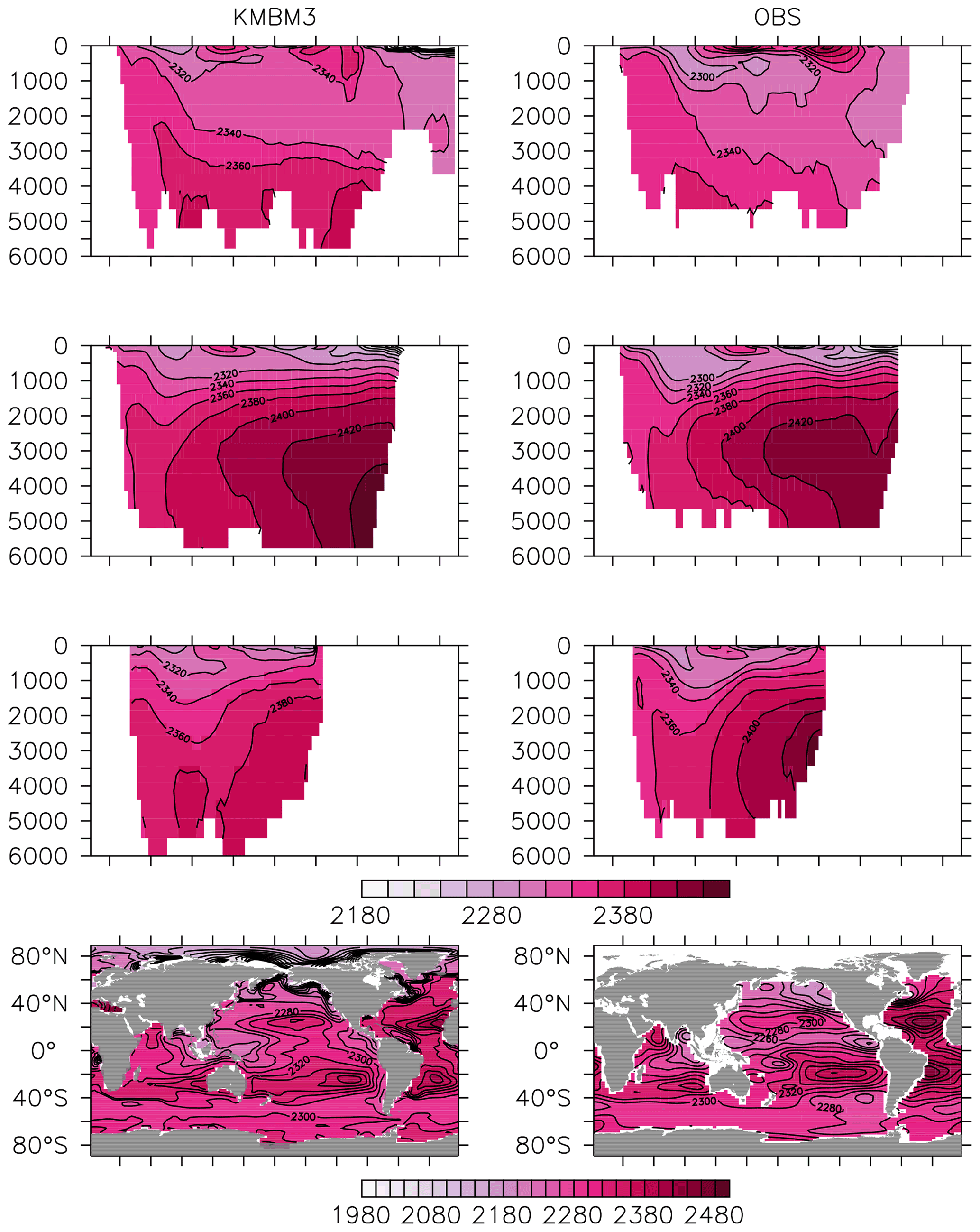
Figure 10Model (left column) year 2014 alkalinity (µmol kg−1) averaged by basin compared to GLODAP (right column; Key et al., 2015; Lauvset et al., 2016). Regions are as follows: Atlantic (top row), Pacific (second row), Indian (third row) and global surface (bottom row).
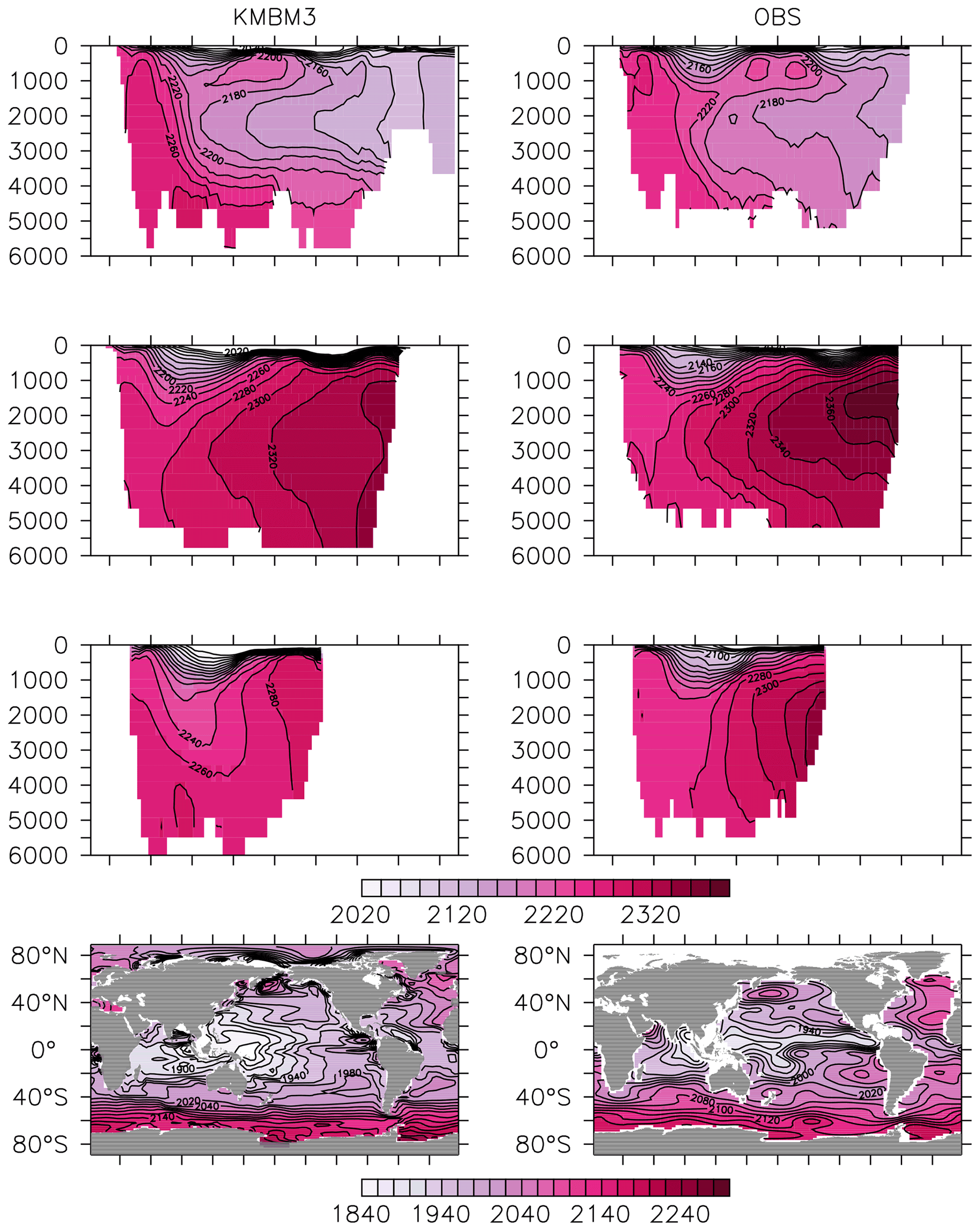
Figure 11Model (left column) year 2014 DIC (µmol kg−1) averaged by basin compared to GLODAP (right column; Key et al., 2015; Lauvset et al., 2016). Regions are as follows: Atlantic (top row), Pacific (second row), Indian (third row) and global surface (bottom row).
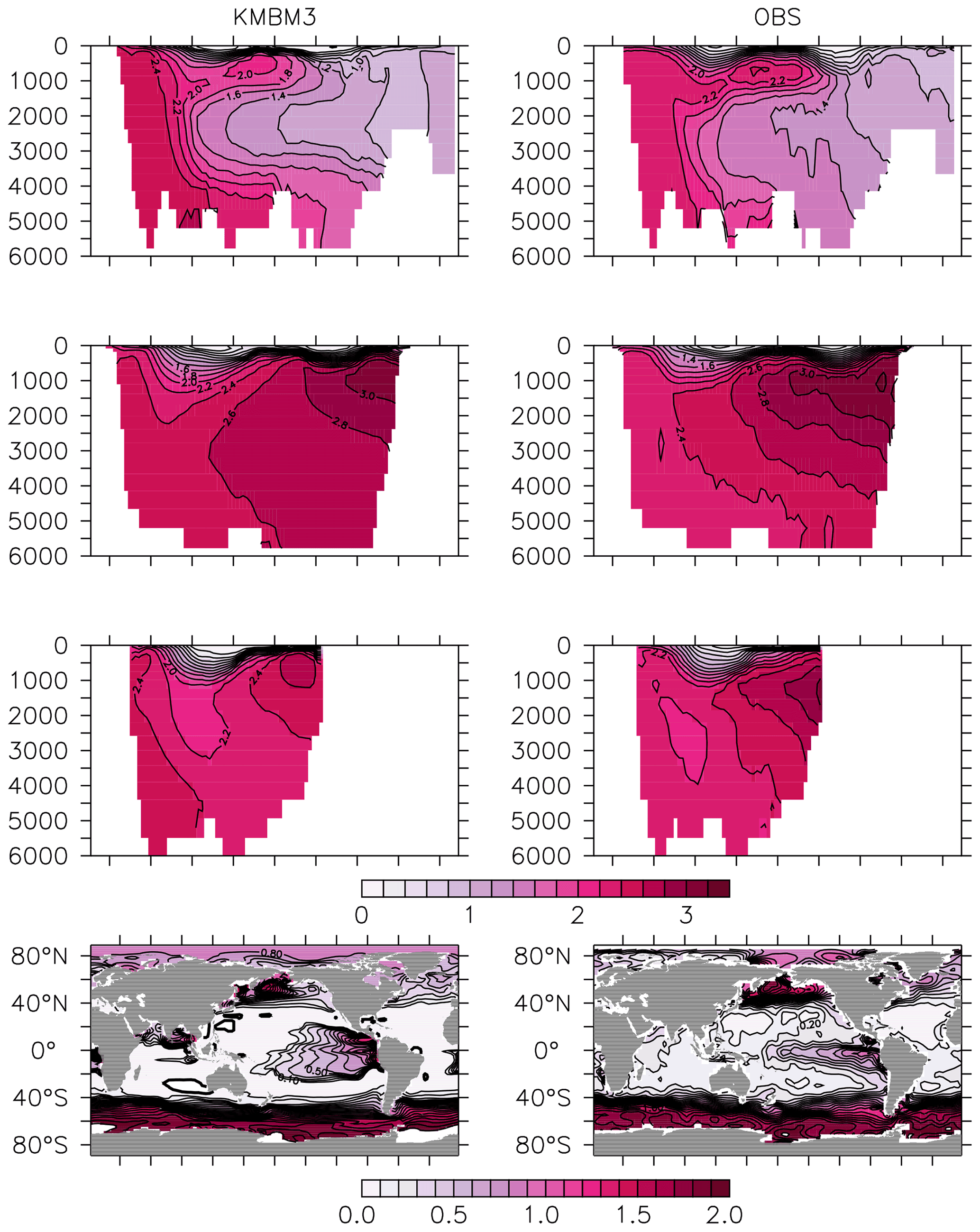
Figure 12Model (left column) year 2014 PO (mmol m−3) averaged by basin compared to WOA (right column; Garcia et al., 2014b). Regions are as follows: Atlantic (top row), Pacific (second row), Indian (third row) and global surface (bottom row).
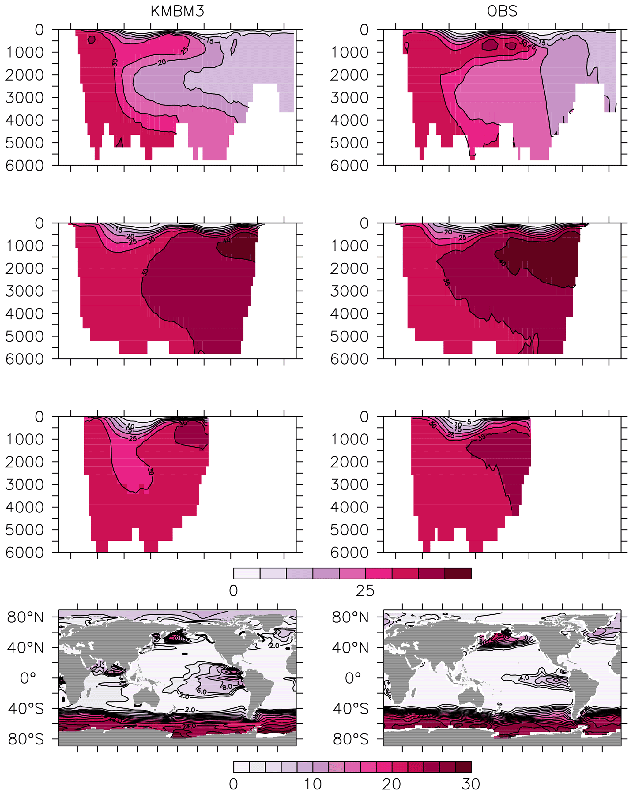
Figure 13Model (left column) year 2014 NO (mmol m−3) averaged by basin compared to WOA (right column; Garcia et al., 2014b). Regions are as follows: Atlantic (top row), Pacific (second row), Indian (third row) and global surface (bottom row).
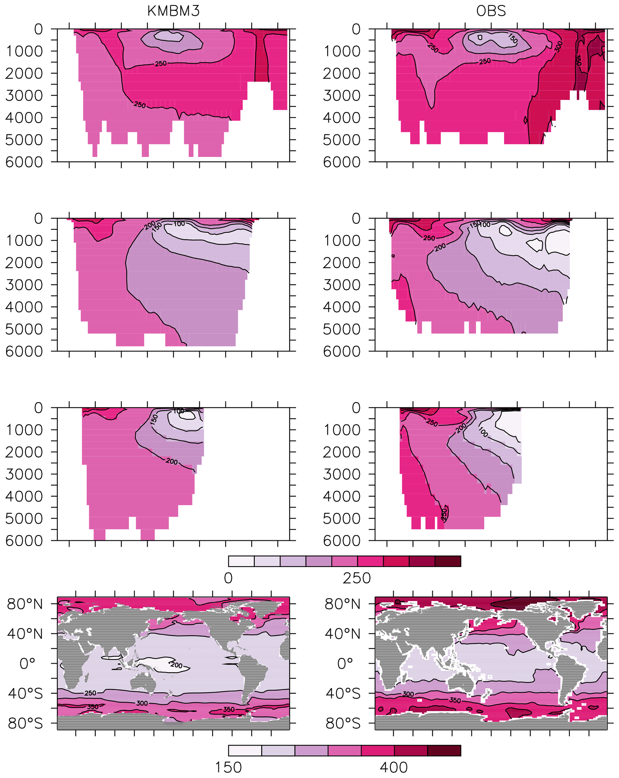
Figure 14Model (left column) year 2014 O2 (mmol m−3) averaged by basin compared to WOA (right column; Garcia et al., 2014a). Regions are as follows: Atlantic (top row), Pacific (second row), Indian (third row) and global surface (bottom row).
Silicic acid distributions are reasonably well captured by the model (Figs. 15, 16). KMBM3 demonstrates the second-highest correlation with gridded observations (Garcia et al., 2014b) of dissolved silicic acid at year 2014 compared to CMIP6 model output (Fig. 16). Two of seven models, MPI-ESM1.2-LR and CMCC-ESM2, have a greater difference in normalized standard deviation than KMBM3. Both correlation and standard deviation are generally better and show less inter-model spread for dissolved silicic acid than for other metrics. KMBM3 simulates the deep Southern Ocean maximum to within 20 mmol Si m−3, with a slight high bias in the deep Atlantic, Pacific and especially Indian sectors (Fig. 15). This spatial weighting to the Indian sector might represent the high bias in diatom biomass in this basin (also clearly seen in the opal flux plots). North Atlantic silicic acid gradients are well represented, while a low bias is apparent in the deep North Pacific of around 20 mmol Si m−3. A low bias is also simulated in the surface North Pacific, which possibly suggests deficiencies in the circulation within and between regional marginal seas (Nishioka et al., 2020). The North Pacific appears to perform well with respect to deep opal flux (Fig. 7), but small biases in fluxes can compound with time in dissolved nutrient fields. It might also be that sedimentary processes that influence deep water silicic acid concentrations would be important to resolve in this region. Our low-bias result in the deep North Pacific is interesting because the origins of the silicic acid-rich deep ocean plume in this region are still under debate (Tréguer and De La Rocha, 2013).
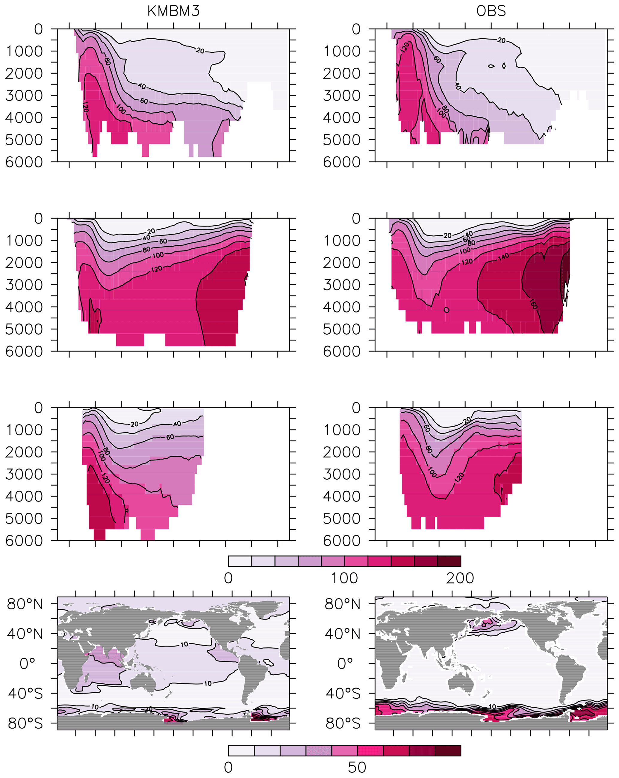
Figure 15Model (left column) year 2014 Si (mmol m−3) averaged by basin compared to WOA (right column; Garcia et al., 2014b). Regions are as follows: Atlantic (top row), Pacific (second row), Indian (third row) and global surface (bottom row).
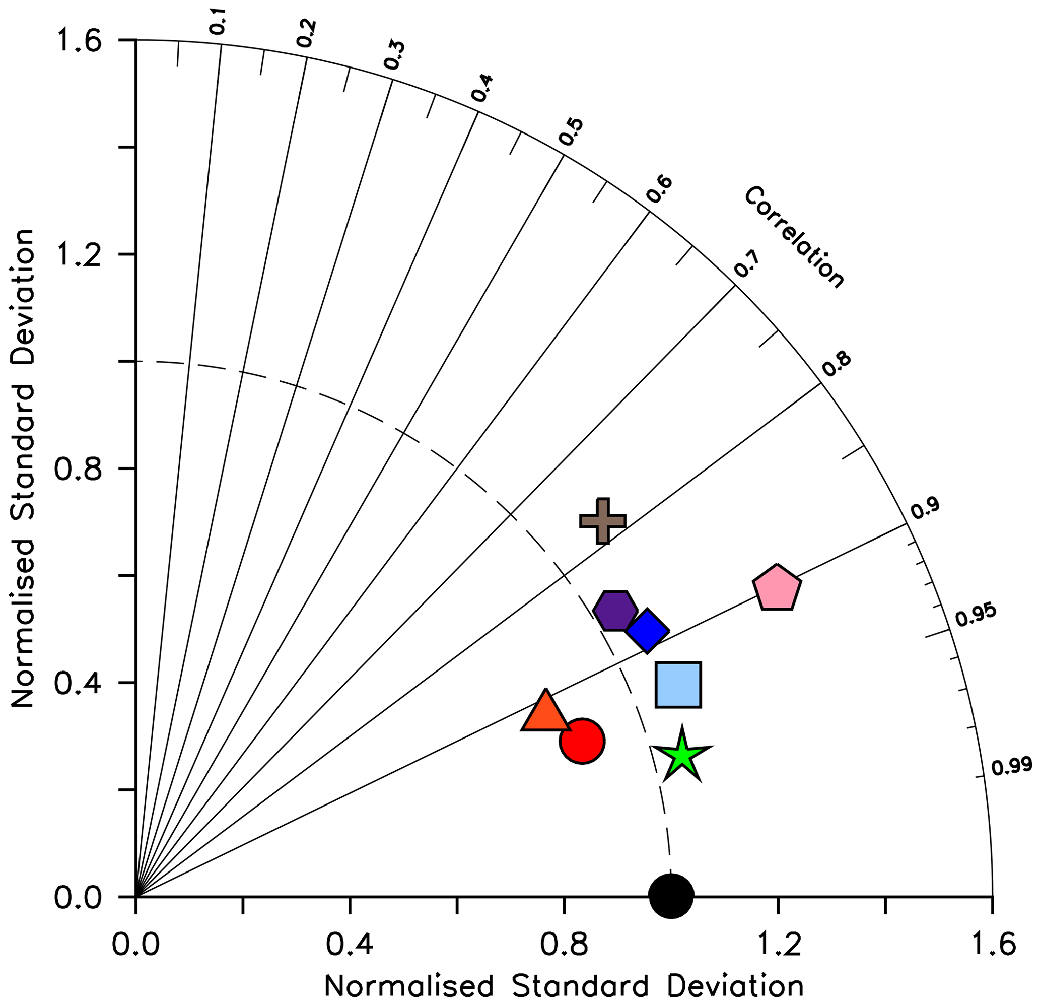
Figure 16Taylor diagram (Taylor, 2001) of CMIP6 annual average dissolved silicic acid distribution (in mol Si m−3) for year 2014, normalized to the Garcia et al. (2014b) dataset. The distance to the origin represents the normalized standard deviation. Normalized correlation with observations is read from the azimuthal position. Perfect agreement with observations is a normalized standard deviation of 1 and a normalized correlation of 1. Models are KMBM3 (red circle), GFDL-ESM4 (green star; Krasting et al., 2018), CESM2 (light blue square; Danabasoglu, 2019), MPI-ESM1.2-LR (pink pentagon; Wieners et al., 2019), NorESM2-LM (brown plus; Seland et al., 2019), CMCC-ESM2 (orange triangle; Lovato et al., 2021), EC-Earth3-CC (blue diamond; EC-Earth Consortium, 2021) and IPSL-CM6A-LR (purple hexagon; Boucher et al., 2018). With the exception of KMBM3, the data for all models were obtained by mining the CMIP6 database (https://esgf-node.llnl.gov/search/cmip6/) using the following search terms: CMIP/si/historical/annual output. Data were accessed between 1–5 February 2021.
Seasonal succession in functional types follows the general progression of zonal maxima in diatoms preceding calcifiers by a few weeks (albeit, in separate zonal ranges, Fig. 17). This succession is due to the higher nutrient requirements, and faster growth rates, of the diatoms, which are able to take advantage of winter mixing early in the growing season. Once surface nutrient concentrations start to decline, the calcifying phytoplankton become relatively more successful. This pattern is most pronounced in the Southern Ocean. In the lower latitudes, diazotroph biomass peaks earlier in the growing season than the low-latitude, non-calcifying phytoplankton (LP). Diazotrophs have a growth handicap with respect to LP, but their ability to fix nitrate gives them an advantage in more stratified summer conditions. This fixed nitrate is then used by the LP in the winter months.

In addition to the historical model forcings described earlier, from the year 2005 to 2300 the simulations are forced using increasing CO2 and non-CO2 greenhouse gas concentrations, projected changes to the fraction of the land surface devoted to agricultural uses (calculated to the year 2100 by Hurtt et al., 2011, and then held constant after) and changes in the direct effect of sulfate aerosols following “business-as-usual” RCP8.5 scenario (RCP8.5, Riahi et al., 2007; Meinshausen et al., 2011). The wind fields continue to be geostrophically adjusted to air temperature anomalies.
4.1 Historical changes (1964–2014)
We next explore model trends from the 1960s to the 2010s and compare to available data from this period. Significant changes are simulated to have already occurred in NPP and phytoplankton biomass, with most of the change over this period occurring since the 1980s (Fig. 18). Global NPP is simulated to have declined 1.4 % between 1964 and 2014, with the strongest declines in the tropics, northern midlatitudes and Southern Ocean due to increasing thermal stratification. In KMBM3, that decline is dominated by the simulated loss of diatom biomass (a 24.4 % decline) due to their high nutrient requirements, largely in the Southern Ocean (Fig. 19). Diazotrophs are simulated to have experienced a 2.0 % loss in biomass globally over this period. Calcifying phytoplankton and low-latitude non-calcifying phytoplankton are simulated to have experienced a 0.4 % and 1.5 % loss, respectively, in net biomass. Increases in calcifying phytoplankton are simulated to have occurred in the Arctic and in the Southern Ocean and decreases are simulated to have occurred in the middle latitudes, where LP have increased their biomass. Warming and a lengthening growing season (but increased stratification; see Arctic temperature trend in Fig. 20) in the Arctic benefit calcifiers. Expansion of coccolithophores into the Arctic has been observed over recent decades (Neukermans et al., 2018). In KMBM3, the Southern Ocean is also simulated to have experienced increasingly favourable conditions for calcifiers, with diatom biomass declining as calcifiers increase. Note, however, that this model does not resolve ocean acidification effects on calcification.
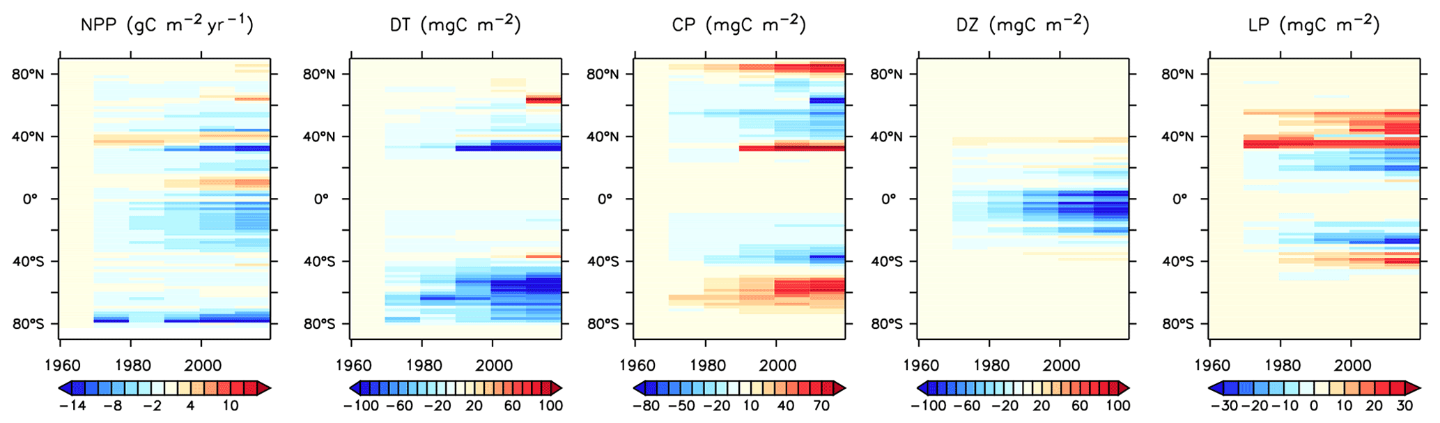
Figure 18Modelled historical changes in zonally averaged and depth-integrated NPP, and phytoplankton biomass, from 1964 to 2014.
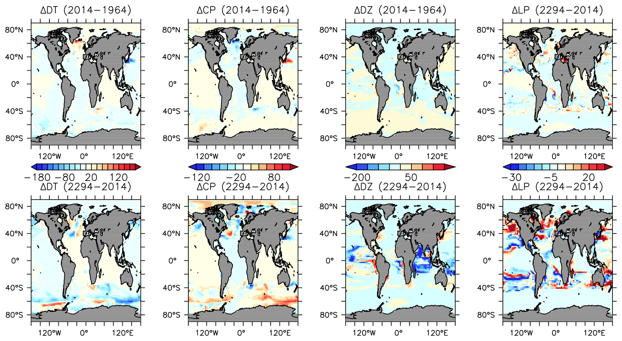
Figure 19Modelled changes in phytoplankton biomass (mmol C m−3) from 1964 to 2014 (top row) and from 2014 to 2294 (bottom row).
KMBM3 simulates a slower global decline in productivity and biomass than the scarce, and controversial, satellite and in situ chlorophyll record reconstructed by Boyce et al. (2010), who calculated a 1 % per year decline in chlorophyll. KMBM3 also does not simulate a large decline prior to the 1950s (Fig. 21). Wernand et al. (2013) found no historical trend in chlorophyll in their Forel–Ule ocean colour scale proxy from 1899 to 2000. However, both chlorophyll reconstructions (and KMBM3) suggest strong regional variation in the historical trends. KMBM3 also simulates a smaller decline in global NPP than an earlier modelling effort, which obtained a 6.5 % decline between 1960–2006 (Laufkötter et al., 2013). Their simulation similarly resulted in large declines in production in the low latitudes, which they attributed to warming and stratification over the historical period. KMBM3 simulates strong warming in the low latitudes (up to 0.5∘ warming in the zonal mean between 1964 and 2014; Fig. 20). Zonal mean trends in idealized natural radiocarbon (simulated without bomb or Suess effects, also Fig. 20) are also positive in the upper ocean, suggesting enhanced stratification and reduced vertical mixing, particularly in the tropical and subtropical Pacific and Indian Ocean basins. Laufkötter et al. (2013) also found strong changes in phytoplankton biogeography in the Southern Ocean and North Atlantic, which they attributed to increasing zonal wind stress and vertical mixing, and surface freshening inducing stratification, respectively. However, our models do not agree in the response of diatoms and high-latitude calcifiers, for which their model simulates high-latitude increases in diatoms. Our results are more similar to those of Rousseaux and Gregg (2015), who combined a model with satellite data to reconstruct ocean surface changes from 1998–2012. They simulated a global decline in diatoms over this period, which they attributed to an increase in nutrient limitation and photosynthetically available radiation, which favours other functional types. However, the Southern Ocean in their model showed no clear trend in phytoplankton community composition between 1998–2012 (Rousseaux and Gregg, 2015). The model we present here is fully competition driven. Variable particle sinking and remineralization rates, and explicit CaCO3 ballasting, further differentiate KMBM3. All of these factors may contribute to the different behaviour reported here.
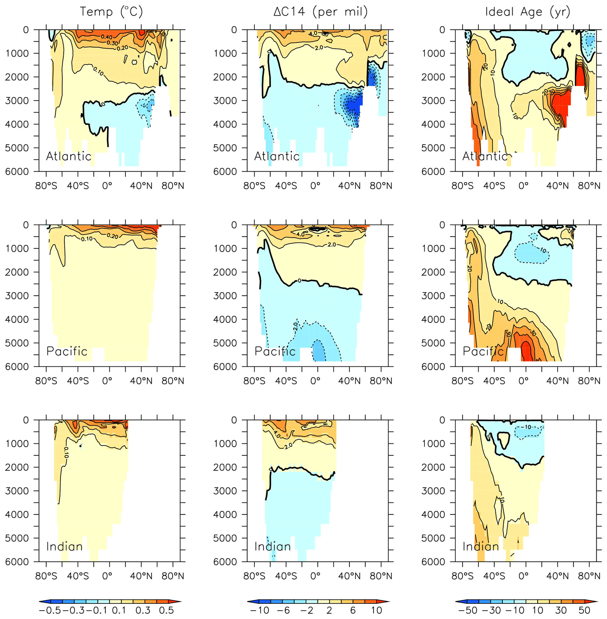
Figure 20Modelled change in temperature, radiocarbon and ideal age profiles by major ocean basins from 1964 to 2014.
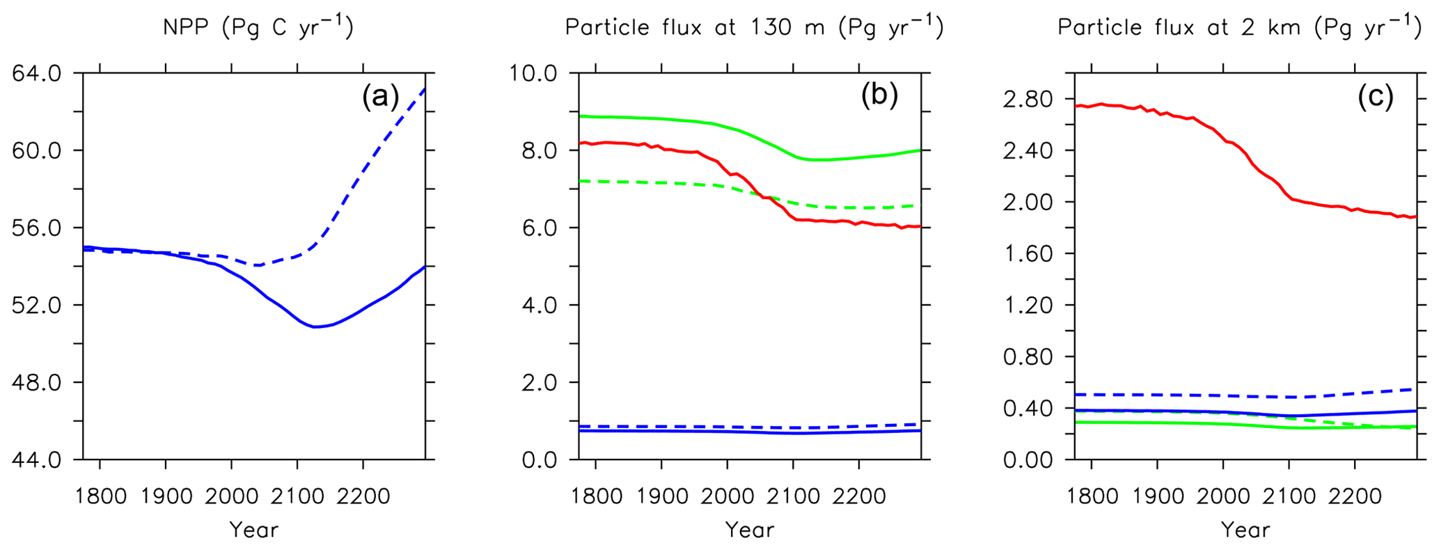
Figure 21Major biogeochemical fluxes in the model, 1776 to 2300. Panel (a) is total net primary production, (b) is total particle fluxes at 130 m depth, (c) is total particle fluxes at 2 km depth. Blue lines in the middle and right panels are PIC, green lines are POC, and red lines are opal. Solid lines are from this model (KMBM3); dashed lines are from the Keller et al. (2012) version (KMBM1).
Trends in biomass and NPP affect deep particle fluxes. Low-latitude declines in primary production result in less deep ocean particle export in the western Pacific and Indian Ocean basins, while deep POC and PIC export is simulated to have slightly increased in the Indian and Pacific sectors of the Southern Ocean and in the Arctic. Trends in deep ocean carbon particle export in KMBM3 generally follow trends in calcifier (CP) biomass (Fig. 19), as CaCO3 (PIC) ballasting contributes significantly to deep export (Kvale et al., 2015a, b, 2019). Declining POC export in the North Atlantic is also simulated to have occurred, though in this region the trend is driven by an increase in diatoms, which are less efficient exporters of organic carbon. Deep ocean opal export is simulated to have declined almost globally, with the largest loss in the Southern Ocean. Opal dissolution is temperature dependent; therefore, regional warming is almost certainly contributing to the reduction of deep ocean opal flux, but the loss of diatom biomass is the major driver of this trend in the Southern Ocean. Global losses of particle export across 2 km depth between 1964 and 2014 are calculated at 2.8 % (POC), 2.2 % (PIC) and 6.2 % (opal).
Unfortunately, there is no comparable historical reconstruction of deep particle fluxes over this time period. Just as with NPP, Laufkötter et al. (2013) simulated a larger decline (8 %) in export production (POC) between 1960 and 2006, which they calculated at 100 m depth. They also simulated the largest declines in the Indian Ocean and west-central Pacific basins, driven by declines in NPP, which in turn were driven by declines in nutrient availability owing to increasing stratification. The models disagree with respect to trends in the North Atlantic, with KMBM3 producing a decline in POC and PIC deep export (due to a decrease in calcifiers), and only a small increase in opal (due to an increase in diatoms). Both Laufkötter et al. (2013) and KMBM3 simulate a historical increase in diatoms in this region; the difference in export trends can be explained by which functional type (calcifiers or diatoms) is more efficient at POC export, with calcifiers being the more efficient carbon exporter in our formulation. Likewise, KMBM3 simulates different POC export trends in the Southern Ocean as Laufkötter et al. (2013), due to differences in model structure. Increasing calcifiers in the Indian sector in KMBM3 increase POC and PIC export there, while in Laufkötter et al. (2013) diatoms regionally increase.
Changes in carbon and nutrient profiles between 1964 and 2014 (Fig. 22) reflect a combination of physical–chemical uptake of anthropogenic CO2 and the changes in ocean circulation on tracer accumulation (Figs. 20 and 24). Dissolved inorganic carbon (DIC) is simulated to have increased by more than 10 mmol C m−3 in zonal mean over this time period in both the Southern Ocean and North Atlantic. Both regions, but particularly the Southern Ocean, are thought to be the primary regions for anthropogenic carbon uptake into the ocean interior (e.g. Khatiwala et al., 2009). The low latitudes are primary regions of carbon storage (Frölicher et al., 2015), and strong (greater than 25 mmol C m−3) increases in DIC are also seen here, in all ocean basins, in the zonal mean profiles.

Figure 22Modelled change in carbon and nutrient profiles by major ocean basins from 1964 to 2014.
Declines in phosphate and nitrate are simulated in the upper ocean in all basins, with the largest zonal mean declines of up to 0.1 mmol P m−3 and 0.5 mmol N m−3). Silicic acid increases by up to 20 mmol Si m−3 in the central North Pacific surface (Fig. 23) due to a regional shift from DT to CP dominance. A recent reconstruction suggests a positive silicate concentration trend in the upper 300 m in this region over the 1970–2017 time period (Stramma et al., 2020), although the estimated magnitude is lower (0.013±0.013 mmol Si m−3 yr−1). Dissolved iron shows an increasing trend in the tropical surface despite using constant atmospheric sources. Surface and subsurface (300 m depth) concentration trends (Fig. 23) reveal spatial heterogeneity, with declining surface and increasing subsurface phosphate occurring in the subarctic North Pacific (a result of increasing particle export) and increasing concentrations along the Humboldt Current (driven by a regional reduction in nitrate; not shown). These results compare favourably with surface declines in phosphate recorded in the North Pacific between 1961 and 2012 (Yasunaka et al., 2016). They also compare favourably with the recent data compilation of Stramma et al. (2020), which shows a decline in surface nutrients, and an increase in subsurface nutrients, in the subarctic Pacific. In KMBM3, this pattern is produced by the replacement of diatoms with calcifiers, who are more efficient exporters of nutrients. The UVic ESCM lacks a fully dynamic atmosphere model and therefore does not simulate multi-decadal oscillations in climate, which have been implicated in recent Pacific interior nutrient trends (Stramma et al., 2020). This may be why KMBM3 does a poor job reproducing observations of nutrient trends observed in the central Pacific (Stramma et al., 2020). Also, increases in nitrate are found in the observed record, which KMBM3 does not simulate. This may be because KMBM3 does not include anthropogenic sources of nitrate (summarized by Stramma et al., 2020).
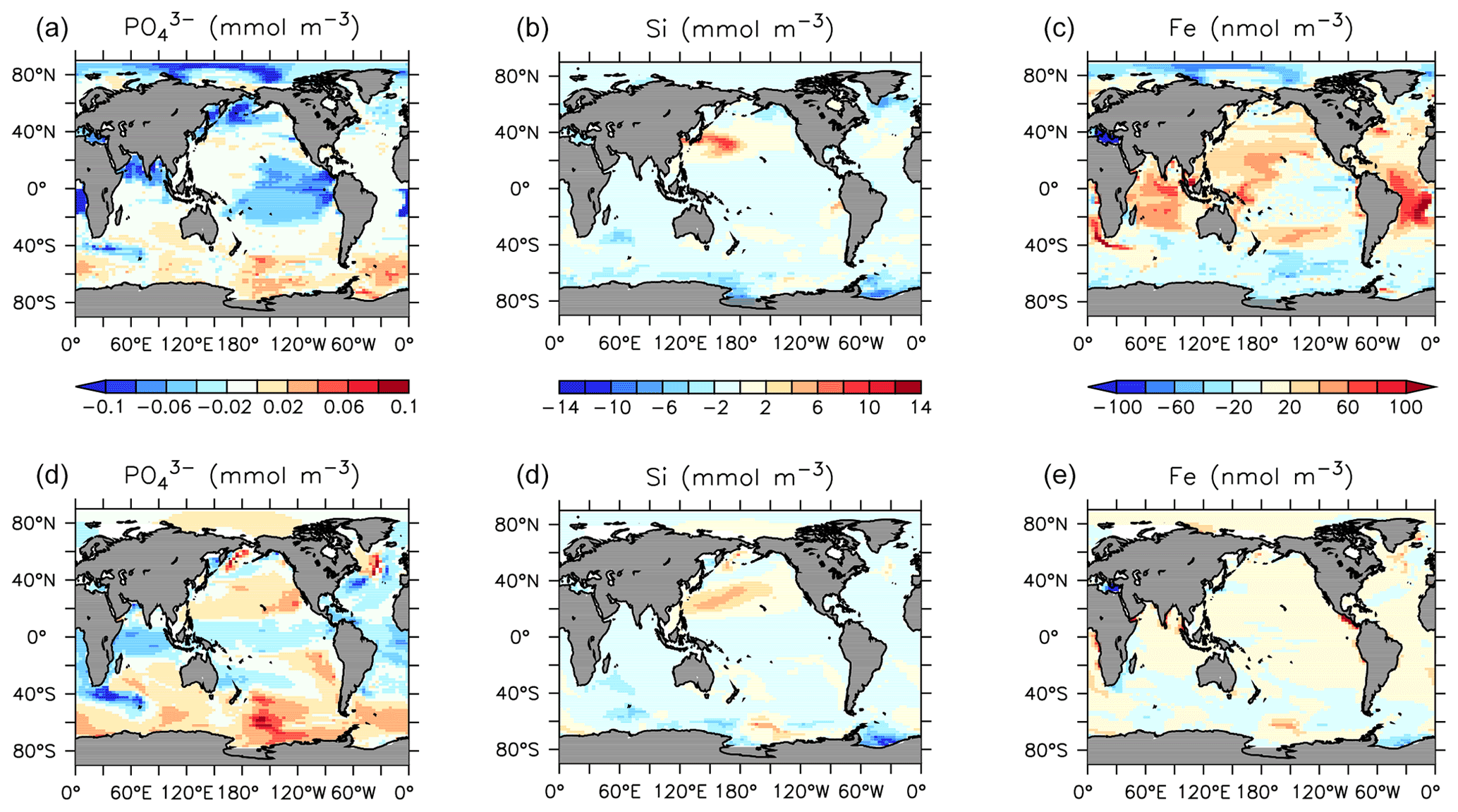
Figure 23Modelled change in nutrients at the surface (a–c) and 300 m depth (d–e) from 1964 to 2014.
Significant increases in North Atlantic deep ocean concentrations (below 3000 m depth) occur in phosphate, nitrate and silicic acid (Fig. 22). A decline in maximum meridional overturning (MOC) of about 1 Sv is apparent over this time, and the water has warmed more than 0.3∘ (Fig. 24). Warming of the Gulf Stream increases particle remineralization rates, thereby raising nutrient concentrations along the North Atlantic Deep Water pathway.
Southern Ocean-sourced intermediate and deep water is simulated to have increased nutrient concentrations from 1964 to 2014, with a positive trend in phosphate and nitrate outcropping along the Antarctic ice margin, in qualitative agreement with the limited observations of an increasing trend in the Indian sector from 1965–2008 (Iida et al., 2013). The Southern Ocean is simulated to have experienced subsurface increases in phosphate in the regions also experiencing increases in silicic acid and iron; this is due to the less efficient export of particles by diatoms (locally increasing over this time), relative to calcifiers.
Taken together, these results suggest declines in NPP and export production upstream of the Southern Ocean have introduced excess nutrients to the basin, raising the nutrient concentrations in Antarctic Bottom and Intermediate water masses despite declining Southern Ocean NPP. These production and export effects have been exacerbated by physical changes in the circulation; Fig. 20 shows a decline in ideal age (greater than 5 years in the zonal mean) in Pacific Intermediate water and the Indian Ocean, which leads to less particle remineralization (and hence, lower nutrient concentrations) there. Increasing water mass age in Southern Ocean-sourced intermediate and deep water masses (upwards of 30 years in the deep Pacific) likewise has the effect of producing more complete particle remineralization, resulting in higher nutrient concentrations.
Oxygen is simulated to have declined in all ocean basins, with the exception of the subsurface low latitudes. It has been previously estimated that the global ocean lost more than 2 % of its oxygen since the 1960s (Schmidtko et al., 2017). KMBM3 simulates a 0.7 % decline in total oxygen content from 1964–2014, which is an under-estimate resulting from physical biases in our model (i.e. deficiencies in simulating low-latitude ventilation), though biogeochemical deficiencies might also be contributing (Oschlies et al., 2017). In the deep ocean, the ageing of water masses (and associated more complete particle remineralization) contributes to the simulated decline in oxygen. In the upper ocean, warming has reduced oxygen solubility, lowering near-surface concentrations.
4.2 Long-term future changes (2014–2294)
More significant changes in ocean biogeochemistry are still to come, if applied boundary forcing assumptions hold over the next centuries. Figures 25 to 28 extend the previous analysis to the year 2294, with respect to 2014 biogeochemistry. Critically, spatial patterns in NPP trends reverse, with strong increases, in places exceeding 80 gC m−2 yr−1 in the zonal mean, in the Southern Ocean (Fig. 25). This trend is dominated by the increase in calcifiers (CP) and, to a lesser geographical extent, diatoms (DT) (Fig. 19). Calcifiers also continue their historical expansion into the Arctic (again, noting adverse physiological effects of ocean acidification are not simulated in this model), while diazotrophs are simulated to significantly increase in the middle latitudes after year 2100. Low-latitude phytoplankton (LP) also broadly increase in biomass between 20∘ S and 60∘ N, though the net NPP trend in the low latitudes remains negative.
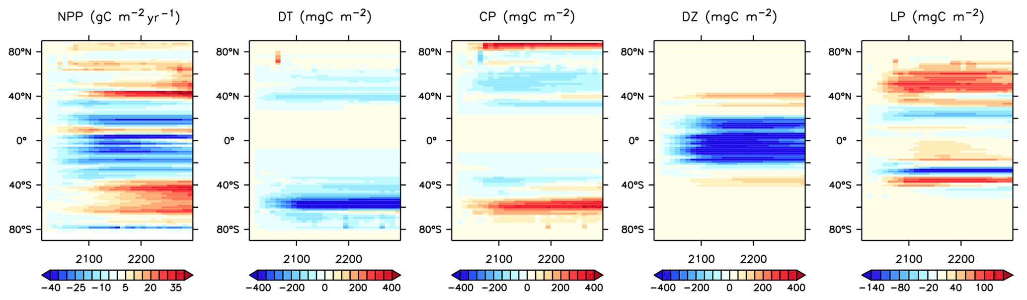
Figure 25Modelled changes in zonally averaged and depth-integrated NPP, and phytoplankton biomass, from 2014 to 2294.
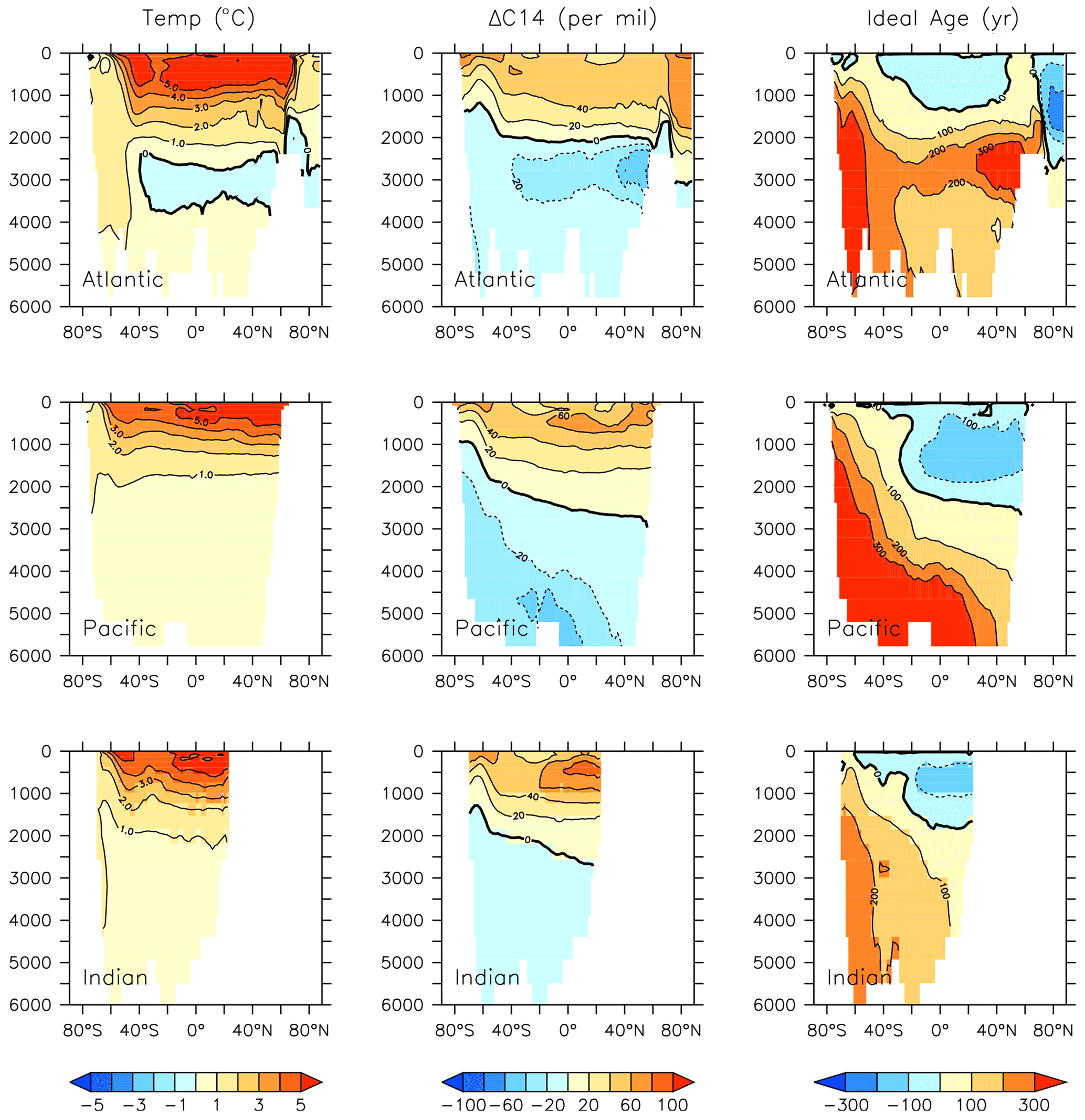
Figure 26Modelled change in temperature, radiocarbon and ideal age profiles by major ocean basins from 2014 to 2296.
This new ecosystem model responds differently to forcing than previous versions. Kvale et al. (2015a) compared the responses of the KMBM1 biogeochemistry (no calcifiers) to two versions of calcifier model, also integrated to 2300 using RCP8.5 forcing, and found the application of calcifiers eliminated the global reduction of NPP found in the Keller et al. (2012) version until around the year 2100. However, the introduction of diatoms and iron, and reorganization of the phytoplankton community structure, produces an even larger decline in global NPP to 2100 (close to 5 Pg C yr−1) in KMBM3 than found in KMBM1 (less than 1 Pg C yr−1). The difference appears to be in the low-latitude response, where calcifiers with low nutrient requirements in the previous version maintained NPP despite stratification, partly by supporting diazotroph nitrogen fixation through efficient ballast removal of surface nitrate (Kvale et al., 2019). In the current model, calcifiers have a lower biomass in the low latitudes and do not establish this symbiotic relationship with diazotrophs to the same extent. As a consequence, diazotrophs decline more strongly than previously. After 2100, NPP increases abruptly (Fig. 21). Rising NPP over the long-term is a long-standing feature of the KMBM biogeochemical model formulation and occurs because of the acceleration of nutrient recycling by the temperature-sensitive microbial loop in the low and middle latitudes (Schmittner et al., 2008). In this latest model version, this increase in NPP is much smaller (less than 4 Pg C yr−1 by 2300, compared to 11–13 Pg C yr−1 in previous model versions). Again, this reduced sensitivity in the low latitudes is due to the reduction of low-latitude ballast-forming calcifiers in the new version. The response of calcifiers outside of the low latitudes to ocean changes is also changed from previous versions, in that our model now simulates increases in biomass in the Southern Ocean as well as the Arctic. Whether these differences are competition effects or due to other model changes, such as the correction of light attenuation, is difficult to assess, but it confirms the finding of Fu et al. (2016) of a strong dependence on phytoplankton community structure in model response to climate change.
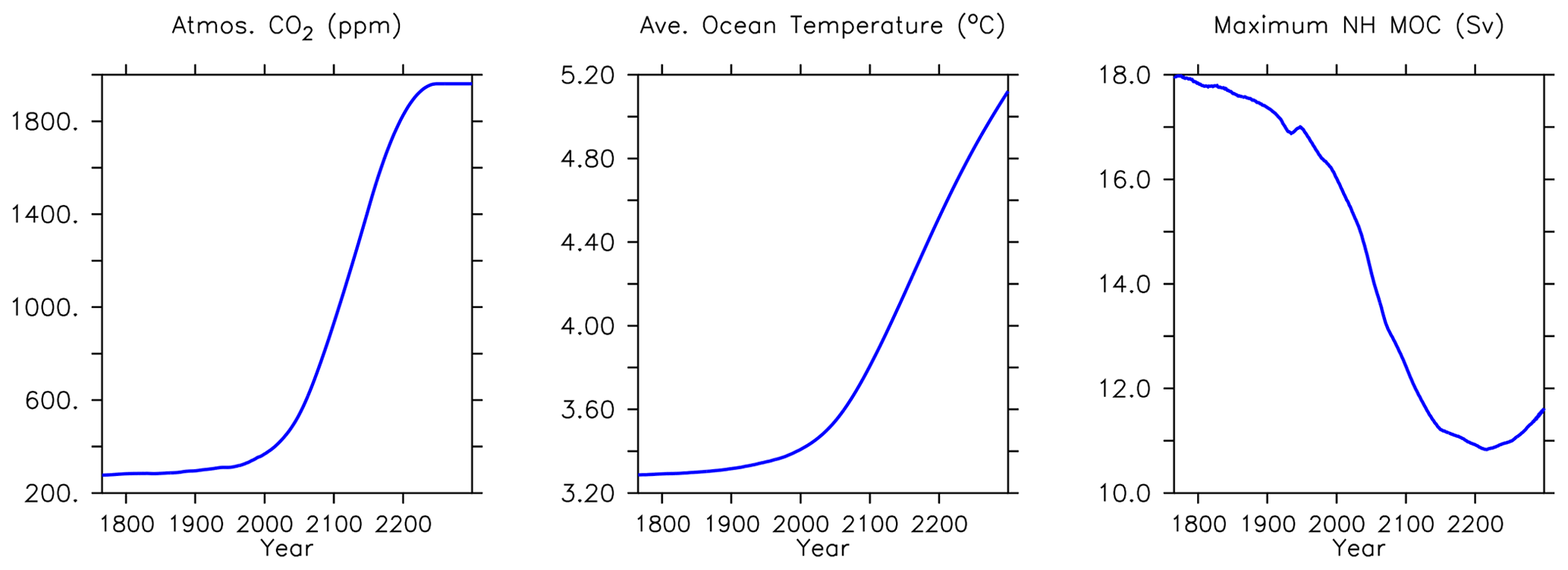
Trends in phytoplankton biomass and productivity can be explained by the physical changes in the model over this time (Figs. 24 and 26). Maximum MOC declines from 18 to 11 Sv over the period 1800 to 2200 before starting to increase after 2200. Slowing overturning helps to accelerate surface warming, and zonal mean temperatures in the upper North Atlantic rise more than 5∘ by 2294. Globally increased radiocarbon in the upper ocean suggests widespread increased stratification, as well as a more complete separation between upper and lower water masses globally (as previously reported by Kvale et al., 2018, with only slightly different forcing conditions). Ideal age trends similarly show the lengthening Southern Ocean-sourced deep water pathway that extends to ventilate all ocean basins from the south, replacing the shoaled northern ventilation pathways (also described in detail in Kvale et al., 2018). Ideal ages increase more than 300 years in the deep southern Pacific and Atlantic basins, and in the deep North Atlantic, where North Atlantic Deep Water formation has declined. The net effect of these physical changes is an overall decline in low-latitude productivity (driven by increased nutrient limitation) but a strong increase in Southern Ocean productivity, with a faster biogeochemical connection between the surface ocean south of the Polar Front and the abyssal basins (see the improved ventilation in the radiocarbon plots). At the poles, fast-growing, nutrient-demanding phytoplankton functional types (DT, CP) thrive, while in the lower latitudes it is the more efficient nutrient consumers (DZ and LP) which benefit.
Long-term particle export trends generally follow the historical trend but with increasing magnitude (Figs. 21 and 27). Globally integrated particle fluxes decline and remain suppressed with respect to pre-industrial rates, for POC and opal. PIC surface export rates change very little and deep export rates increase with climate forcing as a response to increasing surface calcifier POC export fluxes (e.g. Kvale et al., 2015a). The production of both opal and PIC are scaled against their respective plankton types' POC production, so it is expected that PIC and opal fluxes follow the POC export production trend. Just as with NPP, the POC export production decline in KMBM3 is larger than in previous versions (about 2.0 Pg C yr−1 by 2100, rather than 1.5 Pg C yr−1).

Figure 27Modelled change in particle fluxes at 2 km depth, from 2014 to 2294.
POC and PIC fluxes increase where calcifying phytoplankton biomass also increases: south of 40∘ S, in the eastern equatorial Pacific upwelling zone and along the Kuroshio Current into the North Pacific (Fig. 27). Strong decreases in calcifiers, and associated deep carbon export, occur in the Indian Ocean and North Atlantic. Opal export declines by more than 100 mmol Si m−2 yr−1 both south of 40∘ S and north of 40∘ N (with only small changes in the Arctic). However, opal export (and diatoms) increase south of 60∘ S, where increased nutrients (Fig. 28), particularly iron, and a short growing season favours diatoms over calcifiers.
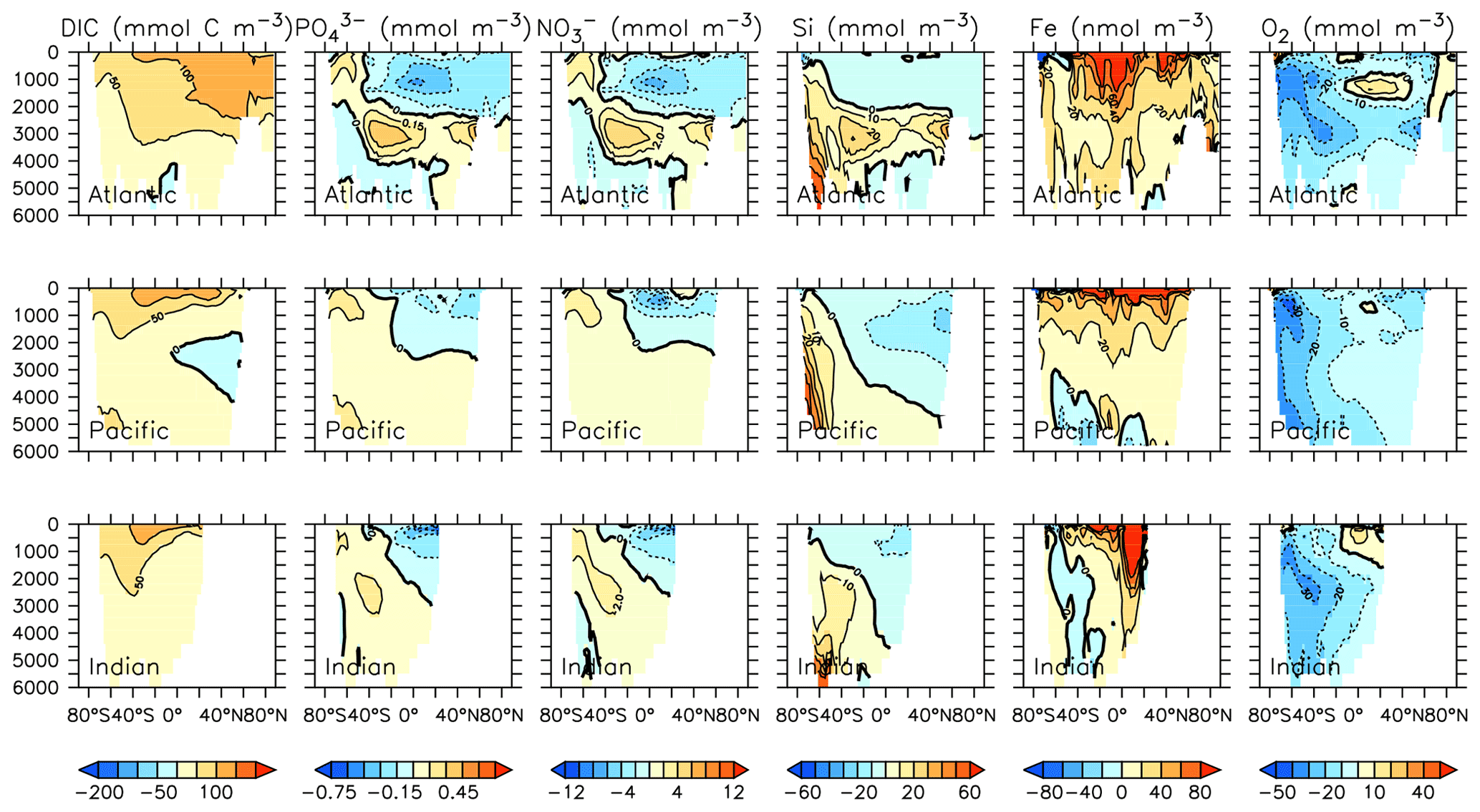
Figure 28Modelled change in carbon and nutrient profiles by major ocean basins from 2014 to 2294.
The historical trend in carbon and nutrients is similarly extended, with continuing increases in DIC in the upper ocean (as atmospheric CO2 continues to enter the ocean), declines in low-latitude upper ocean nutrients phosphate, nitrate and silicic acid (due to decreasing resupply from the deep ocean), increases in the deep ocean in the same nutrients, and widespread declines in oxygen (Fig. 28). Oxygen declines along the Southern Ocean–abyssal global ocean pathway due to both warming and increasing particle remineralization, which is also responsible for the increasing nutrient concentrations in the deep ocean. Decreasing phosphate and nitrate concentrations in the subsurface tropical ocean basins are a product of declining particle remineralization there, brought about by both warming, which shoals remineralization and increases respiration rates and a shift to less efficiently exporting phytoplankton (LP).
The striking trend in dissolved iron that emerges in these future projections of strongly increasing (more than 80 nmol m−3 in the zonal mean) concentrations in the upper ocean was previously described by Nickelsen et al. (2015). They attributed the increase to stratification “trapping” aerosol iron near the surface. However, the regions showing the greatest increases in dissolved iron are also the regions experiencing both strong declines in NPP (and hence, lower iron uptake) and strong declines in particle export (and hence, less particulate iron scavenging and removal). The loss of calcifiers in the Indian Ocean and central Pacific particularly increases iron concentrations there, because of the dual effect of reduced POC and PIC scavenging of iron.
Our future simulation results broadly agree with other long-term simulations in the sustained, and significant, increase in Southern Ocean primary production that couples with a reorganization of deep ocean circulation to produce a long term “nutrient trapping” effect in Southern Ocean-sourced interior water masses (e.g. Moore et al., 2018; Kvale et al., 2019). Near-surface increases in iron, and decreases in nitrate, phosphate and silicic acid, have also been observed to 2100 in a comparison of nine other Earth system models by Fu et al. (2016). These same models also simulate weak to strong increases in diatoms in the Southern Ocean to 2100, though in most, if not all, of them, diatoms are the most efficient exporters of carbon and nutrients (unlike in KMBM3). Phytoplankton community composition and export formulation were discussed by Fu et al. (2016) to be of critical importance in determining trends in NPP, nutrients and particle export over the coming century; thus, a diversity of model formulations benefits our understanding of how the global ocean ecosystem might change in the future.
Our paper describes a new model of the marine silicate cycle (KMBM3), evaluates its performance against previous KMBM versions and other Earth system models, as well as key biogeochemical data derived from observations of the ocean, and compares long-term ecosystem projections to similar models available in the literature. We find our new model shows general improvement in the representation of nutrients and particle fluxes with respect to previous versions of KMBM and is mechanistically more realistic, with the added complexity of iron, calcite and silicate merged into a single model code. Furthermore, its representation of the silicate cycle has similar performance with other state-of-the-art biogeochemical models.
Simulations using our new model suggest diatoms have been, and will continue to be, the losers as the Earth system warms. Their high nutrient requirements prove a disadvantage as the upper ocean stratifies, and small gains in productivity provided by sea ice retreat cannot compensate for the fact that their southern bound is ultimately limited geographically. Calcifying phytoplankton with more moderate nutrient requirements are the big winners across the high latitudes, while in the tropics slow-growing, less-nutrient-hungry phytoplankton are projected to thrive. From a deep ocean carbon sequestration perspective, the loss of diatom export production is of transient importance, as the calcifying phytoplankton increase their role in carbon export, efficiently sinking organic carbon as well as carbonate.
Our simulations also reveal the past may not accurately portray future trends, as evidenced by simulated historical declines in NPP in the Southern Ocean that reverse as conditions become more favourable for calcifiers. Significant and rapid increases in dissolved iron in the low-latitude tropical ocean is another potential biogeochemical “surprise”, still to come, if anthropogenic emissions of carbon follow the present trajectory.
Several aspects of KMBM3, including iron scavenging by calcite, silicate source and sink strengths, and different zooplankton grazing preferences are slated for further study. The impact of variable stoichiometry is another important potential aspect of biogeochemical modelling that is not explored here. More complete parameter assessment is planned in the context of offline parameter optimization and model calibration experiments (e.g. Kriest, 2017; Kriest et al., 2017; Yao et al., 2019) in the future, as is merging this new biogeochemical model into the latest UVic ESCM version (2.10) (Mengis et al., 2020). We look forward to further refinements and the many applications of this model to come.
Data and model code used in the writing of the paper are available on the OPeNDAP GEOMAR server at https://hdl.handle.net/20.500.12085/34412098-27f9-4cbb-992d-12d0d342aa45 (Kvale, 2020). The KMBM3 code released with our paper is only part of all model code required to use the UVic ESCM version 2.9, update 02. The UVic ESCM model code can be found at http://terra.seos.uvic.ca/model/ (Eby, 2021). The KMBM3 code is provided freely but with the requirement that prospective users contact Karin Kvale with their research plans to avoid parallel projects emerging.
Instructions for model use are as follows:
-
The KMBM3 code described, and released, with our paper is only part of all code needed to use the UVic ESCM version 2.9. UVic ESCM 2.9 Updates 02 must be downloaded from http://terra.seos.uvic.ca/model/. Please follow the instructions on this webpage for installation and use.
-
KMBM3 code released with our paper is available at https://hdl.handle.net/20.500.12085/34412098-27f9-4cbb-992d-12d0d342aa45. The code should be called first in the “mk.in” control file, with subsequent calls to the base model code.
KK designed the model and wrote the model code and paper. DPK, WK, CJS and WY contributed model code and bug fixes from previous model versions. KJM and AO contributed to the design of the model. All co-authors contributed to the analysis of the transient simulations and edited the manuscript.
The authors declare that they have no conflict of interest.
Publisher’s note: Copernicus Publications remains neutral with regard to jurisdictional claims in published maps and institutional affiliations.
The authors would like to acknowledge computer resources made available by Kiel University, as well as topical discussion with Michael Eby at the University of Victoria, plotting scripts from Andreas Schmittner (Oregon State University) and Iris Kriest (GEOMAR), plotting scripts and data from Markus Pahlow (GEOMAR), Hannah Geisinger who created a hydrothermal silicate mask, Himadri Saini for code testing and the rest of the Biogeochemical Modelling Department at GEOMAR for their kindness and expertise. Karin Kvale acknowledges support from GEOMAR Helmholtz Centre for Ocean Research, Kiel, and the New Zealand Ministry of Business, Innovation and Employment through the Global Change through Time programme. Katrin J. Meissner acknowledges support from the Australian Research Council (grant nos. DP180100048 and DP180102357). Model tuning was performed in part at the NCI National Facility at the Australian National University, through awards under the National Computational Merit Allocation scheme, the Intersect allocation scheme and the UNSW HPC at NCI scheme. Figure plotting used the Ferret plotting programme. Ferret is a product of NOAA's Pacific Marine Environmental Laboratory.
The article processing charges for this open-access publication were covered by the GEOMAR Helmholtz Centre for Ocean Research Kiel.
This paper was edited by Andrew Yool and reviewed by Mark Baird and two anonymous referees.
Aumont, O., Maier-Reimer, E., Blain, S., and Monfray, P.: An ecosystem model of the global ocean including Fe, Si, P colimitations, Global Biogeochem. Cy., 17, 1060, https://doi.org/10.1029/2001GB001745, 2003. a, b, c, d
Balch, W. M. and Utgoff, P. E.: Potential Interactions Among Ocean Acidification, Coccolithophores, and the Optical Properties of Seawater, Oceanography, 22, 146–159, https://doi.org/10.5670/oceanog.2009.104, 2009. a
Battle, M., Bender, M., Sowers, T., Tans, P., Butler, J., Elkins, J., Ellis, J., Conway, T., Zhang, N., Lang, P., and Clarke, A.: Atmospheric gas concentrations over the past century measured in air from firn at the South Pole, Nature, 383, 231–235, https://doi.org/10.1038/383231a0, 1996. a
Berelson, W. M.: Particle settling rates increase with depth in the ocean, Deep-Sea Res. Pt. II, 49, 237–251, https://doi.org/10.1016/S0967-0645(01)00102-3, 2001. a
Bidle, K. D. and Azam, F.: Accelerated dissolution of diatom silica by marine bacterial assemblages, Nature, 397, 508–512, https://doi.org/10.1038/17351, 1999. a
Boucher, O., Denvil, S., Levavasseur, G., Cozic, A., Caubel, A., Foujols, M.-A., Meurdesoif, Y., Cadule, P., Devilliers, M., Ghattas, J., Lebas, N., Lurton, T., Mellul, L., Musat, I., Mignot, J., and Cheruy, F.: IPSL IPSL-CM6A-LR model output prepared for CMIP6 CMIP historical, Earth System Grid Federation [data set], https://doi.org/10.22033/ESGF/CMIP6.5195, 2018. a, b, c, d
Boyce, D. G., Lewis, M. R., and Worm, B.: Global phytoplankton decline over the past century, Nature, 466, 591–596, https://doi.org/10.1038/nature09268, 2010. a
Buitenhuis, E. T., Vogt, M., Moriarty, R., Bednaršek, N., Doney, S. C., Leblanc, K., Le Quéré, C., Luo, Y.-W., O'Brien, C., O'Brien, T., Peloquin, J., Schiebel, R., and Swan, C.: MAREDAT: towards a world atlas of MARine Ecosystem DATa, Earth Syst. Sci. Data, 5, 227–239, https://doi.org/10.5194/essd-5-227-2013, 2013. a, b, c, d, e
Cael, B. B. and Bisson, K.: Particle Flux Parameterizations: Quantitative and Mechanistic Similarities and Differences, Front. Mar. Sci., 5, 395, https://doi.org/10.3389/fmars.2018.00395, 2018. a
Carr, M.-E., Friedrichs, M. A. M., Schmeltz, M., Aita, M. N., Antoine, D., Arrigo, K. R., Asanuma, I., Aumont, O., Barber, R., Behrenfeld, M., Bidigare, R., Buitenhuis, E. T., Campbell, J., Ciotti, A., Dierssen, H., Dowell, M., Dunne, J., Esaias, W., Gentili, B., Gregg, W., Groom, S., Hoepffner, N., Ishizaka, J., Kameda, T., Le Quéré, C., Lohrenz, S., Marra, J., Melin, F., Moore, K., Morel, A., Reddy, T. E., Ryan, J., Scardi, M., Smyth, T., Turpie, K., Tilstone, G., Waters, K., and Yamanaka, Y.: A comparison of global estimates of marine primary production from ocean color, Deep-Sea Res. Pt. II, 53, 741–770, 2006. a, b
Dale, A. W., Paul, K. M., Clemens, D., Scholz, F., Schroller-Lomnitz, U., Wallmann, K., Geilert, S., Hensen, C., Plass, A., Liebetrau, V., Grasse, P., and Sommer, S.: Recycling and Burial of Biogenic Silica in an Open Margin Oxygen Minimum Zone, Global Biogeochem. Cy., 35, e2020GB006583, https://doi.org/10.1029/2020GB006583, 2021. a
Danabasoglu, G.: NCAR CESM2 model output prepared for CMIP6 CMIP historical, Earth System Grid Federation [data set], https://doi.org/10.22033/ESGF/CMIP6.7627, 2019. a, b, c, d
Eby, M.: Earth System Climate Model, available at: http://terra.seos.uvic.ca/model/, last access: 18 October 2021. a
Eby, M., Zickfeld, K., Montenegro, A., Archer, D., Meissner, K. J., and Weaver, A. J.: Lifetime of Anthropogenic Climate Change: Millennial Time Scales of Potential CO2 and Surface Temperature Perturbations, J. Climate, 22, 2501–2511, https://doi.org/10.1175/2008JCLI2554.1, 2009. a, b, c
EC-Earth Consortium: EC-Earth-Consortium EC-Earth-3-CC model output prepared for CMIP6 CMIP historical, Earth System Grid Federation [data set], https://doi.org/10.22033/ESGF/CMIP6.4702, 2021. a, b, c, d
Enright, C., Buitenhuis, E., and Le Quere, C.: Description of the PlanktTOM10 equations, available at: http://greenocean-data.uea.ac.uk/model/PlankTOM10_Manual.pdf (last access: 5 June 2019), 2014. a, b, c
Eppley, R.: Temperature and phytoplankton growth in the sea, Fish. B. NOAA, 70, 1063—1085, 1972. a
Etheridge, D., Steele, L., Langenfelds, R., Francey, R., Barnola, J., and Morgan, V.: Natural and anthropogenic changes in atmospheric CO2 over the last 1000 years from air in Antarctic ice and firn, J. Geophys. Res.-Atmos., 101, 4115–4128, https://doi.org/10.1029/95JD03410, 1996. a
Etheridge, D., Steele, L., Francey, R., and Langenfelds, R.: Atmospheric methane between 1000 AD and present: Evidence of anthropogenic emissions and climatic variability, J. Geophys. Res.-Atmos., 103, 15979–15993, https://doi.org/10.1029/98JD00923, 1998. a
Ferretti, D., Miller, J., White, J., Etheridge, D., Lassey, K., Lowe, D., Meure, C., Dreier, M., Trudinger, C., van Ommen, T., and Langenfelds, R.: Unexpected changes to the global methane budget over the past 2000 years, Science, 309, 1714–1717, https://doi.org/10.1126/science.1115193, 2005. a
Flückiger, J., Dällenbach, A., Blunier, T., Stauffer, B., Stocker, T. F., Raynaud, D., and Barnola, J.-M.: Variations in atmospheric N2O concentration during abrupt climatic changes, Science, 285, 227–230, https://doi.org/10.1126/science.285.5425.227, 1999. a
Flückiger, J., Blunier, T., Stauffer, B., Chappellaz, J., Spahni, R., Kawamura, K., Schwander, J., Stocker, T. F., and Dahl-Jensen, D.: N2O and CH4 variations during the last glacial epoch: Insight into global processes, Global Biogeochem. Cy., 18, GB1020, https://doi.org/10.1029/2003GB002122, 2004. a
Frölicher, T. L., Sarmiento, J. L., Paynter, D. J., Dunne, J. P., Krasting, J. P., and Winton, M.: Dominance of the Southern Ocean in Anthropogenic Carbon and Heat Uptake in CMIP5 Models, J. Climate, 28, 862–886, https://doi.org/10.1175/JCLI-D-14-00117.1, 2015. a
Fu, W., Randerson, J. T., and Moore, J. K.: Climate change impacts on net primary production (NPP) and export production (EP) regulated by increasing stratification and phytoplankton community structure in the CMIP5 models, Biogeosciences, 13, 5151–5170, https://doi.org/10.5194/bg-13-5151-2016, 2016. a, b, c
Galbraith, E. D., Gnanadesikan, A., Dunne, J. P., and Hiscock, M. R.: Regional impacts of iron-light colimitation in a global biogeochemical model, Biogeosciences, 7, 1043–1064, https://doi.org/10.5194/bg-7-1043-2010, 2010. a
Garcia, H., Locarnini, R. A., Boyer, T. P., Antonov, J., Baranova, O., Zweng, M. M., Reagan, J., and Johnson, D.: World Ocean Atlas 2013, Volume 3: Dissolved Oxygen, Apparent Oxygen Utilization, and Oxygen Saturation, Tech. rep., NOAA Atlas NESDIS 75, U.S. Government Printing Office, Washington, D.C., 2014a. a, b, c
Garcia, H., Locarnini, R. A., Boyer, T. P., Antonov, J., Zweng, M. M., Reagan, J., Baranova, O., and Johnson, D.: World Ocean Atlas 2013, Volume 4: Dissolved Inorganic Nutrients (phosphate, nitrate, silicate), Tech. rep., NOAA Atlas NESDIS 76, U.S. Government Printing Office, Washington, D.C., 2014b. a, b, c, d, e, f, g
Gnanadesikan, A.: A global model of silicon cycling: Sensitivity to eddy parameterization and dissolution, Global Biogeochem. Cy., 13, 199–220, https://doi.org/10.1029/1998GB900013, 1999. a, b, c
Heinze, C., Eyring, V., Friedlingstein, P., Jones, C., Balkanski, Y., Collins, W., Fichefet, T., Gao, S., Hall, A., Ivanova, D., Knorr, W., Knutti, R., Löw, A., Ponater, M., Schultz, M. G., Schulz, M., Siebesma, P., Teixeira, J., Tselioudis, G., and Vancoppenolle, M.: ESD Reviews: Climate feedbacks in the Earth system and prospects for their evaluation, Earth Syst. Dynam., 10, 379–452, https://doi.org/10.5194/esd-10-379-2019, 2019. a
Holzer, M., Primeau, F. W., DeVries, T., and Matear, R.: The Southern Ocean silicon trap: Data-constrained estimates of regenerated silicic acid, trapping efficiencies, and global transport paths, J. Geophys. Res.-Oceans, 119, 313–331, https://doi.org/10.1002/2013JC009356, 2014. a, b
Honjo, S., Manganini, S. J., Krishfield, R. A., and Francois, R.: Particulate organic carbon fluxes to the ocean interior and factors controlling the biological pump: A synthesis of global sediment trap programs since 1983, Prog. Oceanogr., 76, 217–285, 2008. a, b, c, d, e, f
Hurtt, G. C., Chini, L. P., Frolking, S., Betts, R. A., Feddema, J., Fischer, G., Fisk, J. P., Hibbard, K., Houghton, R. A., Janetos, A., Jones, C. D., Kindermann, G., Kinoshita, T., Klein Goldewijk, K., Riahi, K., Shevliakova, E., Smith, S., Stehfest, E., Thomson, A., Thornton, P., van Vuuren, D. P., and Wang, Y. P.: Harmonization of land-use scenarios for the period 1500–2100: 600 years of global gridded annual land-use transitions, wood harvest, and resulting secondary lands, Climatic Change, 109, 117, https://doi.org/10.1007/s10584-011-0153-2, 2011. a
Iida, T., Odate, T., and Fukuchi, M.: Long-Term Trends of Nutrients and Apparent Oxygen Utilization South of the Polar Front in Southern Ocean Intermediate Water from 1965 to 2008, PLOS ONE, 8, 1–7, https://doi.org/10.1371/journal.pone.0071766, 2013. a
Jin, X., Gruber, N., Dunne, J. P., Sarmiento, J. L., and Armstrong, R. A.: Diagnosing the contribution of phytoplankton functional groups to the production and export of particulate organic carbon, CaCO3, and opal from global nutrient and alkalinity distributions, Global Biogeochem. Cy., 20, GB2015, https://doi.org/10.1029/2005GB002532, 2006. a, b, c
Kalnay, E., Kanamitsu, M., Kistler, R., Collins, W., Deaven, D., Gandin, L., Iredell, M., Saha, S., White, G., Woollen, J., Zhu, Y., Chelliah, M., Ebisuzaki, W., Higgins, W., Janowiak, J., Mo, K., Ropelewski, C., Wang, J., Leetmaa, A., Reynolds, R., Jenne, R., and Joseph, D.: The NCEP/NCAR 40-year reanalysis project, B. Am. Meteorol. Soc., 77, 437–471, https://doi.org/10.1175/1520-0477(1996)077<0437:TNYRP>2.0.CO;2, 1996. a
Keller, D. P., Oschlies, A., and Eby, M.: A new marine ecosystem model for the University of Victoria Earth System Climate Model, Geosci. Model Dev., 5, 1195–1220, https://doi.org/10.5194/gmd-5-1195-2012, 2012. a, b, c, d, e, f, g, h, i, j, k, l, m, n, o, p, q, r, s, t, u
Key, R., Olsen, A., van Heuven, S., Lauvset, A., Velo, Lin, X., Schirnick, C., Kozyr, A., Tanhua, T., Hoppema, M., Jutterström, S., Steinfeldt, R., Jeansson, E., Ishii, M., Perez, F. F., and Suzuki, T.: Global Ocean Data Analysis Project, Version 2 (GLODAPv2), Tech. rep., US Department of Energy, Carbon Dioxide Information Analysis Center, Oak Ridge National Laboratory, US Department of Energy, Oak Ridge, Tennessee [data set], https://doi.org/10.3334/CDIAC/OTG.NDP093_GLODAPv2, 2015. a, b, c, d
Khatiwala, S.: A computational framework for simulation of biogeochemical tracers in the ocean, Global Biogeochem. Cy., 21, GB3001, https://doi.org/10.1029/2007GB002923, 2007. a
Khatiwala, S., Primeau, F., and Hall, T.: Reconstruction of the history of anthropogenic CO2 concentrations in the ocean, Nature, 462, 346–349, https://doi.org/10.1038/nature08526, 2009. a
Khatiwala, S., Visbeck, M., and Cane, M.: Accelerated simulation of passive tracers in ocean circulation models, Ocean Model., 9, 51–69, https://doi.org/10.1016/j.ocemod.2004.04.002, 2005. a
Koeve, W., Wagner, H., Kähler, P., and Oschlies, A.: 14C-age tracers in global ocean circulation models, Geosci. Model Dev., 8, 2079–2094, https://doi.org/10.5194/gmd-8-2079-2015, 2015. a
Krasting, J. P., John, J. G., Blanton, C., McHugh, C., Nikonov, S., Radhakrishnan, A., Rand, K., Zadeh, N. T., Balaji, V., Durachta, J., Dupuis, C., Menzel, R., Robinson, T., Underwood, S., Vahlenkamp, H., Dunne, K. A., Gauthier, P. P., Ginoux, P., Griffies, S. M., Hallberg, R., Harrison, M., Hurlin, W., Malyshev, S., Naik, V., Paulot, F., Paynter, D. J., Ploshay, J., Schwarzkopf, D. M., Seman, C. J., Silvers, L., Wyman, B., Zeng, Y., Adcroft, A., Dunne, J. P., Dussin, R., Guo, H., He, J., Held, I. M., Horowitz, L. W., Lin, P., Milly, P., Shevliakova, E., Stock, C., Winton, M., Xie, Y., and Zhao, M.: NOAA-GFDL GFDL-ESM4 model output prepared for CMIP6 CMIP historical, Earth System Grid Federation [data set], https://doi.org/10.22033/ESGF/CMIP6.8597, 2018. a, b, c, d
Kriest, I.: Calibration of a simple and a complex model of global marine biogeochemistry, Biogeosciences, 14, 4965–4984, https://doi.org/10.5194/bg-14-4965-2017, 2017. a, b
Kriest, I. and Oschlies, A.: Numerical effects on organic-matter sedimentation and remineralization in biogeochemical ocean models, Ocean Model., 39, 275–283, https://doi.org/10.1016/j.ocemod.2011.05.001, 2011. a
Kriest, I., Sauerland, V., Khatiwala, S., Srivastav, A., and Oschlies, A.: Calibrating a global three-dimensional biogeochemical ocean model (MOPS-1.0), Geosci. Model Dev., 10, 127–154, https://doi.org/10.5194/gmd-10-127-2017, 2017. a, b
Kriest, I., Kähler, P., Koeve, W., Kvale, K., Sauerland, V., and Oschlies, A.: One size fits all? Calibrating an ocean biogeochemistry model for different circulations, Biogeosciences, 17, 3057–3082, https://doi.org/10.5194/bg-17-3057-2020, 2020. a
Kvale, K.: Supplementary Data to “Explicit silicate cycling in the Kiel Marine Biogeochemistry Model, version 3 (KMBM3) embedded in the UVic ESCM version 2.9”, OPeNDAP GEOMAR serve [code and data set], available at: https://hdl.handle.net/20.500.12085/34412098-27f9-4cbb-992d-12d0d342aa45 (last access: 18 October 2021), 2020. a
Kvale, K. F. and Meissner, K. J.: Primary production sensitivity to phytoplankton light attenuation parameter increases with transient forcing, Biogeosciences, 14, 4767–4780, https://doi.org/10.5194/bg-14-4767-2017, 2017. a
Kvale, K. F., Khatiwala, S., Dietze, H., Kriest, I., and Oschlies, A.: Evaluation of the transport matrix method for simulation of ocean biogeochemical tracers, Geosci. Model Dev., 10, 2425–2445, https://doi.org/10.5194/gmd-10-2425-2017, 2017. a, b, c
Kvale, K. F., Turner, K. E., Keller, D. P., and Meissner, K. J.: Asymmetric dynamical ocean responses in warming icehouse and cooling greenhouse climates, Environ. Res. Lett., 13, 125011, https://doi.org/10.1088/1748-9326/aaedc3, 2018. a, b
Kvale, K. F., Turner, K. E., Landolfi, A., and Meissner, K. J.: Phytoplankton calcifiers control nitrate cycling and the pace of transition in warming icehouse and cooling greenhouse climates, Biogeosciences, 16, 1019–1034, https://doi.org/10.5194/bg-16-1019-2019, 2019. a, b, c
Kvale, K. F., Meissner, K. J., and Keller, D. P.: Potential increasing dominance of heterotrophy in the global ocean, Environ. Res. Lett., 10, 074009, https://doi.org/10.1088/1748-9326/10/7/074009, 2015a. a, b, c, d, e, f, g, h
Kvale, K. F., Meissner, K. J., Keller, D. P., Eby, M., and Schmittner, A.: Explicit Planktic Calcifiers in the University of Victoria Earth System Climate Model, Version 2.9, Atmosphere-Ocean, 53, 332–350, https://doi.org/10.1080/07055900.2015.1049112, 2015b. a, b, c, d, e, f, g, h, i, j, k, l, m
Laufkötter, C., Vogt, M., and Gruber, N.: Long-term trends in ocean plankton production and particle export between 1960–2006, Biogeosciences, 10, 7373–7393, https://doi.org/10.5194/bg-10-7373-2013, 2013. a, b, c, d, e, f
Lauvset, S. K., Key, R. M., Olsen, A., van Heuven, S., Velo, A., Lin, X., Schirnick, C., Kozyr, A., Tanhua, T., Hoppema, M., Jutterström, S., Steinfeldt, R., Jeansson, E., Ishii, M., Perez, F. F., Suzuki, T., and Watelet, S.: A new global interior ocean mapped climatology: the 1∘ × 1∘ GLODAP version 2, Earth Syst. Sci. Data, 8, 325–340, https://doi.org/10.5194/essd-8-325-2016, 2016. a, b, c, d
Leblanc, K., Arístegui Ruiz, J., Armand, L. K., Assmy, P., Beker, B., Bode, A., Breton, E., Cornet, V., Gibson, J., Gosselin, M.-P., Kopczynska, E. E., Marshall, H. G., Peloquin, J. M., Piontkovski, S., Poulton, A. J., Quéguiner, B., Schiebel, R., Shipe, R., Stefels, J., van Leeuwe, M. A., Varela, M., Widdicombe, C. E., and Yallop, M.: Global distributions of diatoms abundance, biovolume and biomass – Gridded data product (NetCDF) – Contribution to the MAREDAT World Ocean Atlas of Plankton Functional Types, PANGAEA [data set], https://doi.org/10.1594/PANGAEA.777384, 2012. a, b, c, d
Lovato, T., Peano, D., and Butenschön, M.: CMCC CMCC-ESM2 model output prepared for CMIP6 CMIP historical, Earth System Grid Federation [data set], https://doi.org/10.22033/ESGF/CMIP6.13195, 2021. a, b, c, d
Luo, Y.-W., Doney, S. C., Anderson, L. A., Benavides, M., Berman-Frank, I., Bode, A., Bonnet, S., Boström, K. H., Böttjer, D., Capone, D. G., Carpenter, E. J., Chen, Y. L., Church, M. J., Dore, J. E., Falcón, L. I., Fernández, A., Foster, R. A., Furuya, K., Gómez, F., Gundersen, K., Hynes, A. M., Karl, D. M., Kitajima, S., Langlois, R. J., LaRoche, J., Letelier, R. M., Marañón, E., McGillicuddy Jr., D. J., Moisander, P. H., Moore, C. M., Mouriño-Carballido, B., Mulholland, M. R., Needoba, J. A., Orcutt, K. M., Poulton, A. J., Rahav, E., Raimbault, P., Rees, A. P., Riemann, L., Shiozaki, T., Subramaniam, A., Tyrrell, T., Turk-Kubo, K. A., Varela, M., Villareal, T. A., Webb, E. A., White, A. E., Wu, J., and Zehr, J. P.: Database of diazotrophs in global ocean: abundance, biomass and nitrogen fixation rates, Earth Syst. Sci. Data, 4, 47–73, https://doi.org/10.5194/essd-4-47-2012, 2012. a, b, c
Luo, Y.-W., Lima, I. D., Karl, D. M., Deutsch, C. A., and Doney, S. C.: Data-based assessment of environmental controls on global marine nitrogen fixation, Biogeosciences, 11, 691–708, https://doi.org/10.5194/bg-11-691-2014, 2014. a, b
Machida, T., Nakazawa, T., Fujii, Y., Aoki, S., and Watanabe, O.: Increase in the atmospheric nitrous-oxide concentration during the last 250 years, Geophys. Res. Lett., 22, 2921–2924, https://doi.org/10.1029/95GL02822, 1995. a
Mahowald, N. M., Muhs, D. R., Levis, S., Rasch, P. J., Yoshioka, M., Zender, C. S., and Luo, C.: Change in atmospheric mineral aerosols in response to climate: Last glacial period, preindustrial, modern, and doubled carbon dioxide climates, J. Geophys. Res.-Atmos., 111, https://doi.org/10.1029/2005JD006653, 2006. a
Matsumoto, K., Sarmiento, J. L., and Brzezinski, M. A.: Silicic acid leakage from the Southern Ocean: A possible explanation for glacial atmospheric pCO2, Global Biogeochem. Cy., 16, 5-1–5-23, https://doi.org/10.1029/2001GB001442, 2002. a
Meinshausen, M., Smith, S. J., Calvin, K., Daniel, J. S., Kainuma, M. L. T., Lamarque, J.-F., Matsumoto, K., Montzka, S. A., Raper, S. C. B., Riahi, K., Thomson, A., Velders, G. J. M., and van Vuuren, D. P. P.: The RCP greenhouse gas concentrations and their extensions from 1765 to 2300, Climatic Change, 109, 213–241, https://doi.org/10.1007/s10584-011-0156-z, 2011. a
Meissner, K., Weaver, A., Matthews, H., and Cox, P.: The role of land surface dynamics in glacial inception: A study with the UVic Earth System Model, Clim. Dynam., 21, 515–537, https://doi.org/10.1007/s00382-003-0352-2, 2003. a
Mengis, N., Keller, D. P., MacDougall, A. H., Eby, M., Wright, N., Meissner, K. J., Oschlies, A., Schmittner, A., MacIsaac, A. J., Matthews, H. D., and Zickfeld, K.: Evaluation of the University of Victoria Earth System Climate Model version 2.10 (UVic ESCM 2.10), Geosci. Model Dev., 13, 4183–4204, https://doi.org/10.5194/gmd-13-4183-2020, 2020. a
Merico, A., Tyrrell, T., and Cokacar, T.: Is there any relationship between phytoplankton seasonal dynamics and the carbonate system?, J. Marine Syst., 59, 120–142, 2006. a
Meure, M. C., Etheridge, D., Trudinger, C., Steele, P., Langenfelds, R., van Ommen, T., Smith, A., and Elkins, J.: Law Dome CO2, CH4 and N2O ice core records extended to 2000 years BP, Geophys. Res. Lett., 33, L14810, https://doi.org/10.1029/2006GL026152, 2006. a
Moore, J. K., Fu, W., Primeau, F., Britten, G. L., Lindsay, K., Long, M., Doney, S. C., Mahowald, N., Hoffman, F., and Randerson, J. T.: Sustained climate warming drives declining marine biological productivity, Science, 359, 1139–1143, https://doi.org/10.1126/science.aao6379, 2018. a
Muglia, J., Somes, C. J., Nickelsen, L., and Schmittner, A.: Combined Effects of Atmospheric and Seafloor Iron Fluxes to the Glacial Ocean, Paleoceanography, 32, 1204–1218, https://doi.org/10.1002/2016PA003077, 2017. a, b, c, d
NASA (NASA Goddard Space Flight Center, Ocean Ecology Laboratory, Ocean Biology Processing Group): Moderate-resolution Imaging Spectroradiometer (MODIS) Aqua Particulate Inorganic Carbon Data, 2018 Reprocessing, NASA OB.DAAC, Greenbelt, MD, USA [data set], https://doi.org/data/10.5067/AQUA/MODIS/L3M/PIC/2018, 2018. a, b, c
Neukermans, G., Oziel, L., and Babin, M.: Increased intrusion of warming Atlantic water leads to rapid expansion of temperate phytoplankton in the Arctic, Glob. Change Biol., 24, 2545–2553, https://doi.org/10.1111/gcb.14075, 2018. a
Nickelsen, L., Keller, D. P., and Oschlies, A.: A dynamic marine iron cycle module coupled to the University of Victoria Earth System Model: the Kiel Marine Biogeochemical Model 2 for UVic 2.9, Geosci. Model Dev., 8, 1357–1381, https://doi.org/10.5194/gmd-8-1357-2015, 2015 a, b, c, d, e, f, g, h, i, j, k, l, m, n, o, p, q
Nishioka, J., Obata, H., Ogawa, H., Ono, K., Yamashita, Y., Lee, K., Takeda, S., and Yasuda, I.: Subpolar marginal seas fuel the North Pacific through the intermediate water at the termination of the global ocean circulation, P. Natl. Acad. Sci. USA, 117, 12665–12673, https://doi.org/10.1073/pnas.2000658117, 2020. a
Olsson, J., Stipp, S., Makovicky, E., and Gislason, S.: Metal scavenging by calcium carbonate at the Eyjafjallajökull volcano: A carbon capture and storage analogue, Chem. Geol., 384, 135–148, https://doi.org/10.1016/j.chemgeo.2014.06.025, 2014. a
Oschlies, A., Duteil, O., Getzlaff, J., Koeve, W., Landolfi, A., and Schmidtko, S.: Patterns of deoxygenation: sensitivity to natural and anthropogenic drivers, Philos. T. R. Soc. A, 375, 20160325, https://doi.org/10.1098/rsta.2016.0325, 2017. a, b
O'Brien, C. J.: Global distributions of coccolithophores abundance and biomass – Gridded data product (NetCDF) – Contribution to the MAREDAT World Ocean Atlas of Plankton Functional Types, PANGAEA [data set], https://doi.org/10.1594/PANGAEA.785092, 2012. a, b, c
Paasche, E.: A review of the coccolithophorid Emiliania huxleyi (Prymnesiophyceae), with particular reference to growth, coccolith formation, and calcification-photosynthesis interactions, Phycologia, 40, 503–529, 2001. a
Partanen, A., Keller, D. P., Korhonen, H., and Matthews, H. D.: Impacts of sea spray geoengineering on ocean biogeochemistry, Geophys. Res. Lett., 43, 7600–7608, https://doi.org/10.1002/2016GL070111, 2016. a
Pasquier, B. and Holzer, M.: Inverse-model estimates of the ocean's coupled phosphorus, silicon, and iron cycles, Biogeosciences, 14, 4125–4159, https://doi.org/10.5194/bg-14-4125-2017, 2017. a
Renaudie, J.: Quantifying the Cenozoic marine diatom deposition history: links to the C and Si cycles, Biogeosciences, 13, 6003–6014, https://doi.org/10.5194/bg-13-6003-2016, 2016. a
Riahi, K., Gruebler, A., and Nakicenovic, N.: Scenarios of long-term socio-economic and environmental development under climate stabilization, Technol. Forecast. Soc., 74, 887–935, https://doi.org/10.1016/j.techfore.2006.05.026, 2007. a
Ridgwell, A., Watson, A., and Archer, D.: Modeling the response of the oceanic Si inventory to perturbation, and consequences for atmospheric CO2, Global Biogeochem. Cy., 16, 19-1–19-25, https://doi.org/10.1029/2002GB001877, 2002. a, b
Rousseaux, C. S. and Gregg, W. W.: Recent decadal trends in global phytoplankton composition, Global Biogeochem. Cy., 29, 1674–1688, https://doi.org/10.1002/2015GB005139, 2015. a, b
Sarmiento, J. and Gruber, N.: Ocean Biogeochemical Dynamics, Princeton University Press, Princeton and Oxford, 2006. a, b, c, d
Schmidtko, S., Stramma, L., and Visbeck, M.: Decline in global oceanic oxygen content during the past five decades, Nature, 542, 335–339, https://doi.org/10.1038/nature21399, 2017. a
Schmittner, A., Oschlies, A., Giraud, X., Eby, M., and Simmons, H.: A global model of the marine ecosystem for long-term simulations: Sensitivity to ocean mixing, buoyancy forcing, particle sinking, and dissolved organic matter cycling, Global Biogeochem. Cy., 19, GB3004, https://doi.org/10.1029/2004GB002283, 2005. a, b, c
Schmittner, A., Oschlies, A., Matthews, H. D., and Galbraith, E. D.: Future changes in climate, ocean circulation, ecosystems, and biogeochemical cycling simulated for a business-as-usual CO2 emission scenario until year 4000 AD, Global Biogeochem. Cy., 22, GB1013, https://doi.org/10.1029/2007GB002953, 2008. a, b, c, d, e
Seland, y., Bentsen, M., Oliviè, D. J. L., Toniazzo, T., Gjermundsen, A., Graff, L. S., Debernard, J. B., Gupta, A. K., He, Y., Kirkevåg, A., Schwinger, J., Tjiputra, J., Aas, K. S., Bethke, I., Fan, Y., Griesfeller, J., Grini, A., Guo, C., Ilicak, M., Karset, I. H. H., Landgren, O. A., Liakka, J., Moseid, K. O., Nummelin, A., Spensberger, C., Tang, H., Zhang, Z., Heinze, C., Iversen, T., and Schulz, M.: NCC NorESM2-LM model output prepared for CMIP6 CMIP historical, Earth System Grid Federation [data set], https://doi.org/10.22033/ESGF/CMIP6.8036, 2019. a
Smith, S. V. and Gattuso, J.-P.: Balancing the Oceanic Calcium Carbonate Cycle: Consequences of Variable Water Column Ψ, Aquat. Geochem., 17, 327–337, https://doi.org/10.1007/s10498-010-9109-9, 2011. a
Smith, S. V. and Mackenzie, F. T.: The Role of CaCO3 Reactions in the Contemporary Oceanic CO2 Cycle, Aquat. Geochem., 22, 153–175, https://doi.org/10.1007/s10498-015-9282-y, 2016. a
Somes, C. J., Oschlies, A., and Schmittner, A.: Isotopic constraints on the pre-industrial oceanic nitrogen budget, Biogeosciences, 10, 5889–5910, https://doi.org/10.5194/bg-10-5889-2013, 2013. a, b
Stramma, L., Schmidtko, S., Bograd, S. J., Ono, T., Ross, T., Sasano, D., and Whitney, F. A.: Trends and decadal oscillations of oxygen and nutrients at 50 to 300 m depth in the equatorial and North Pacific, Biogeosciences, 17, 813–831, https://doi.org/10.5194/bg-17-813-2020, 2020. a, b, c, d, e
Swart, N. C., Cole, J. N., Kharin, V. V., Lazare, M., Scinocca, J. F., Gillett, N. P., Anstey, J., Arora, V., Christian, J. R., Jiao, Y., Lee, W. G., Majaess, F., Saenko, O. A., Seiler, C., Seinen, C., Shao, A., Solheim, L., von Salzen, K., Yang, D., Winter, B., and Sigmond, M.: CCCma CanESM5-CanOE model output prepared for CMIP6 CMIP historical, Earth System Grid Federation [data set], https://doi.org/10.22033/ESGF/CMIP6.10260, 2019. a, b
Taylor, K. E.: Summarizing multiple aspects of model performance in a single diagram, J. Geophys. Res.-Atmos., 106, 7183–7192, https://doi.org/10.1029/2000JD900719, 2001. a, b, c
Tréguer, P., Bowler, C., Moriceau, B., Dutkiewicz, S., Gehlen, M., Aumont, O., Bittner, L., Dugdale, R., Finkel, Z., Iudicone, D., Jahn, O., Guidi, L., Lasbleiz, M., Leblanc, K., Levy, M., and Pondaven, P.: Influence of diatom diversity on the ocean biological carbon pump, Nat. Geosci., 11, 27–37, https://doi.org/10.1038/s41561-017-0028-x, 2018. a
Tréguer, P. J. and De La Rocha, C. L.: The World Ocean Silica Cycle, Annu. Rev. Mar. Sci., 5, 477–501, https://doi.org/10.1146/annurev-marine-121211-172346, 2013. a, b, c, d, e, f
Tréguer, P. J., Sutton, J. N., Brzezinski, M., Charette, M. A., Devries, T., Dutkiewicz, S., Ehlert, C., Hawkings, J., Leynaert, A., Liu, S. M., Llopis Monferrer, N., López-Acosta, M., Maldonado, M., Rahman, S., Ran, L., and Rouxel, O.: Reviews and syntheses: The biogeochemical cycle of silicon in the modern ocean, Biogeosciences, 18, 1269–1289, https://doi.org/10.5194/bg-18-1269-2021, 2021. a, b, c, d, e, f, g, h, i, j, k
Van Cappellen, P., Dixit, S., and van Beusekom, J.: Biogenic silica dissolution in the oceans: Reconciling experimental and field-based dissolution rates, Global Biogeochem. Cy., 16, 23-1–23-10, https://doi.org/10.1029/2001GB001431, 2002. a
Weaver, A., Eby, M., Wiebe, E., Bitz, C., Duffy, P., Ewen, T., Fanning, A., Holland, M., MacFadyen, A., Matthews, H., Meissner, K., Saenko, O., Schmittner, A., Wang, H., and Yoshimori, M.: The UVic Earth System Climate Model: Model description, climatology, and applications to past, present and future climates, Atmosphere-Ocean, 39, 361–428, 2001. a, b, c
Weber, T. and Deutsch, C.: Oceanic nitrogen reservoir regulated by plankton diversity and ocean circulation, Nature, 489, 419, https://doi.org/10.1038/nature11357 2012. a
Wernand, M. R., van der Woerd, H. J., and Gieskes, W. W. C.: Trends in Ocean Colour and Chlorophyll Concentration from 1889 to 2000, Worldwide, PLOS ONE, 8, 1–20, https://doi.org/10.1371/journal.pone.0063766, 2013. a
Westberry, T., Behrenfeld, M. J., Siegel, D. A., and Boss, E.: Carbon-based primary productivity modeling with vertically resolved photoacclimation, Global Biogeochem. Cy., 22, GB2024, https://doi.org/10.1029/2007GB003078, 2008. a
Wieners, K.-H., Giorgetta, M., Jungclaus, J., Reick, C., Esch, M., Bittner, M., Legutke, S., Schupfner, M., Wachsmann, F., Gayler, V., Haak, H., de Vrese, P., Raddatz, T., Mauritsen, T., von Storch, J.-S., Behrens, J., Brovkin, V., Claussen, M., Crueger, T., Fast, I., Fiedler, S., Hagemann, S., Hohenegger, C., Jahns, T., Kloster, S., Kinne, S., Lasslop, G., Kornblueh, L., Marotzke, J., Matei, D., Meraner, K., Mikolajewicz, U., Modali, K., Müller, W., Nabel, J., Notz, D., Peters, K., Pincus, R., Pohlmann, H., Pongratz, J., Rast, S., Schmidt, H., Schnur, R., Schulzweida, U., Six, K., Stevens, B., Voigt, A., and Roeckner, E.: MPI-M MPI-ESM1.2-LR model output prepared for CMIP6 CMIP historical, Earth System Grid Federation [data set], https://doi.org/10.22033/ESGF/CMIP6.6595, 2019. a, b
Yao, W., Kvale, K. F., Achterberg, E., Koeve, W., and Oschlies, A.: Hierarchy of calibrated global models reveals improved distributions and fluxes of biogeochemical tracers in models with explicit representation of iron, Environ. Res. Lett., 14, 114009, https://doi.org/10.1088/1748-9326/ab4c52, 2019. a, b, c
Yasunaka, S., Ono, T., Nojiri, Y., Whitney, F. A., Wada, C., Murata, A., Nakaoka, S., and Hosoda, S.: Long-term variability of surface nutrient concentrations in the North Pacific, Geophys. Res. Lett., 43, 3389–3397, https://doi.org/10.1002/2016GL068097, 2016. a
Zhang, Y., Mahowald, N., Scanza, R. A., Journet, E., Desboeufs, K., Albani, S., Kok, J. F., Zhuang, G., Chen, Y., Cohen, D. D., Paytan, A., Patey, M. D., Achterberg, E. P., Engelbrecht, J. P., and Fomba, K. W.: Modeling the global emission, transport and deposition of trace elements associated with mineral dust, Biogeosciences, 12, 5771–5792, https://doi.org/10.5194/bg-12-5771-2015, 2015. a
The requested paper has a corresponding corrigendum published. Please read the corrigendum first before downloading the article.
- Article
(20048 KB) - Full-text XML