the Creative Commons Attribution 4.0 License.
the Creative Commons Attribution 4.0 License.
 | 05 Nov 2021
Testing stomatal models at the stand level in deciduous angiosperm and evergreen gymnosperm forests using CliMA Land (v0.1)
Philipp Köhler
Liyin He
Russell Doughty
Renato K. Braghiere
Jeffrey D. Wood
Christian Frankenberg
At the leaf level, stomata control the exchange of water and carbon across the air–leaf interface. Stomatal conductance is typically modeled empirically, based on environmental conditions at the leaf surface. Recently developed stomatal optimization models show great skills at predicting carbon and water fluxes at both the leaf and tree levels. However, how well the optimization models perform at larger scales has not been extensively evaluated. Furthermore, stomatal models are often used with simple single-leaf representations of canopy radiative transfer (RT), such as big-leaf models. Nevertheless, the single-leaf canopy RT schemes do not have the capability to model optical properties of the leaves nor the entire canopy. As a result, they are unable to directly link canopy optical properties with light distribution within the canopy to remote sensing data observed from afar. Here, we incorporated one optimization-based and two empirical stomatal models with a comprehensive RT model in the land component of a new Earth system model within CliMA, the Climate Modelling Alliance. The model allowed us to simultaneously simulate carbon and water fluxes as well as leaf and canopy reflectance and fluorescence spectra. We tested our model by comparing our modeled carbon and water fluxes and solar-induced chlorophyll fluorescence (SIF) to two flux tower observations (a gymnosperm forest and an angiosperm forest) and satellite SIF retrievals, respectively. All three stomatal models quantitatively predicted the carbon and water fluxes for both forests. The optimization model, in particular, showed increased skill in predicting the water flux given the lower error (ca. 14.2 % and 21.8 % improvement for the gymnosperm and angiosperm forests, respectively) and better 1:1 comparison (slope increases from ca. 0.34 to 0.91 for the gymnosperm forest and from ca. 0.38 to 0.62 for the angiosperm forest). Our model also predicted the SIF yield, quantitatively reproducing seasonal cycles for both forests. We found that using stomatal optimization with a comprehensive RT model showed high accuracy in simulating land surface processes. The ever-increasing number of regional and global datasets of terrestrial plants, such as leaf area index and chlorophyll contents, will help parameterize the land model and improve future Earth system modeling in general.
- Article
(8567 KB) - Full-text XML
-
Supplement
(9594 KB) - BibTeX
- EndNote


© 2021 California Institute of Technology. Government sponsorship acknowledged.
Anthropogenic emissions have resulted in an unprecedentedly rapid increase in the atmospheric carbon dioxide (CO2) concentration and thus global warming (IPCC, 2014). The land system, a big carbon sink (Quéré et al., 2018; Friedlingstein et al., 2020), slows the increase in atmospheric [CO2] and climate change by taking up about one-third of anthropogenic emissions. Yet, whether the land system continues to be a carbon sink in the near future remains debatable (Anav et al., 2013; Arora et al., 2013; Jones et al., 2013; Sperry et al., 2019). Increasing tree mortality across the globe further complicates this prediction (Hartmann et al., 2015). A key to addressing this problem is to better simulate and monitor the coupled carbon, water, and energy fluxes at the land surface.
Terrestrial plants control the opening of tiny pores on leaves, called stomata, in response to a variety of environmental and physiological stimuli. Therefore, accurately representing this process is essential in land surface simulations, as stomata affect carbon and water fluxes as well as the surface energy balance. In the past decades, many stomatal models, based either on statistical regressions (e.g., Ball et al., 1987; Leuning, 1995; Medlyn et al., 2011) or optimization theories (e.g., Cowan and Farquhar, 1977; Wolf et al., 2016; Sperry et al., 2017; Mencuccini et al., 2019; Wang et al., 2020), have been proposed and used to model leaf-level stomatal responses. The empirical models are computationally efficient and skillfully represent stomatal responses to the environmental cues in the absence of water stress; thus, they are widely used in land surface models (LSMs). However, these empirical models rely on ad hoc tuning factors to force stomatal response to drought (Powell et al., 2013), which introduces additional uncertainty in carbon cycle modeling (Trugman et al., 2018).
In comparison, trait-based stomatal optimization models predict stomatal behavior based on the trade-off between the benefits of carbon gain and the risk of water loss from the stomatal opening (Wolf et al., 2016; Wang et al., 2020). For instance, when the soil gets drier, the risk of transporting the same amount of water increases due to a higher risk of xylem cavitation (Sperry et al., 2017), while the carbon gain remains unchanged. As a result, plants ought to reduce stomatal opening and, thus, water loss to balance gain and risk. A major advantage of stomatal optimization models is that they couple environmental stress (from both the atmosphere and soil) to plant physiology; thus, they more accurately represent mechanistic processes while also being less dependent on statistically fitted parameters. In particular, stomatal optimization models based on plant hydraulics have shown great potential in predicting leaf- and tree-level stomatal behavior at multiple scales, ranging from potted saplings to common garden and natural forest stands (Anderegg et al., 2018; Venturas et al., 2018; Wang et al., 2019; Liu et al., 2020). Also, attempts to employ the optimization theory at the regional scale have shown improved predictive skills compared with empirical stomatal models (Eller et al., 2020; Sabot et al., 2020). Furthermore, optimization theory can be readily extended to explain and model nighttime stomatal responses to the environment (Wang et al., 2021).
While traits used in stomatal optimization models improve predictive skill, the number of traits required to parameterize these process- and trait-based models makes it impractical to apply them at large spatial scales. As a result, stomatal optimization models have not been rigorously evaluated at the stand level or larger spatial scales. Eddy covariance measurements of carbon, water vapor, energy exchange, and environmental conditions give a good estimate of stand-level fluxes and provide a platform to test stomatal theories at the ecosystem level (Baldocchi et al., 2001; Baldocchi, 2020). Despite the often unknown plant traits and species composition within a flux tower footprint, continuous and high-quality data make it possible to invert a suite of average stand-level traits. However, more investigation is required to determine how well the stomatal optimization models perform at the stand level, which is a gap that this paper aims to address.
If high-quality flux tower data are used (such as a full suite of environmental conditions and carbon and water fluxes), the traits required to run stomatal optimization models can be inverted from flux tower observations. However, the sparse distribution of flux towers across the globe may be too sparse to provide a good estimate of how traits vary globally (Schimel et al., 2015), thereby impeding the implementation of stomatal optimization theory at the landscape level. Although it is possible to interpolate these traits using climate as a driving force, as done by Jung et al. (2020), these interpolated parameters cannot be verified in terms of carbon and water flux measurements directly. The growing amount of remote sensing data, such as canopy reflectance and fluorescence-based products, provides an alternative way to verify model parameterization (Schimel et al., 2019). For instance, solar-induced chlorophyll fluorescence (SIF) and near-infrared reflectance of vegetation correlate with plant productivity (Frankenberg et al., 2011; Sun et al., 2018; Badgley et al., 2019). Furthermore, it is possible to directly compare model-predicted reflectance and fluorescence spectra to satellite observations.
To date, all stomatal optimization models are used with simple canopy radiative transfer (RT) schemes due to their simplicity and efficiency (including the big-leaf model, which partitions the canopy into sunlit and shaded fractions; Campbell and Norman, 1998). The single-leaf representation of the canopy, however, is not adequate in modern LSMs in terms of simulating the reflectance or fluorescence of the entire canopy, which requires bidirectional radiation within the canopy to be simulated. Therefore, more complex models with multiple canopy layers, horizontal canopy heterogeneity (Braghiere et al., 2021), and more detailed representations of the canopy RT scheme are required for the purpose of simulating canopy optical parameters, such as the RT scheme used in the Soil Canopy Observation of Photosynthesis and Energy fluxes (SCOPE) model (Yang et al., 2017). This way, the advantages of stomatal optimization theory and those of a complicated multilayer canopy RT scheme are integrated, being able to better relate plant physiology to remotely sensed canopy spectra.
Here, we aim to advance land surface modeling by incorporating a recently developed stomatal optimization model (Wang et al., 2020) and the SCOPE RT concept in the land system of a new generation of Earth system model within the Climate Modeling Alliance (CliMA). With the CliMA Land model, we were able to link both plant productivity and canopy optical parameters to stomatal optimization theory. We evaluated our model by comparing the model-predicted ecosystem carbon and water fluxes to flux tower measurements as well as to two well-established empirical stomatal models, and comparing the model-predicted SIF to the TROPOspheric Monitoring Instrument (TROPOMI) SIF retrievals (Köhler et al., 2018).
We present our first step towards bridging stomatal control, plant hydraulics, and a comprehensive RT scheme in the land component of a new Earth system model developed by the Climate Modeling Alliance (CliMA). The CliMA Land model addresses soil water movement, plant water transport, stomatal regulation, canopy radiative transfer, and water, carbon, and energy fluxes in a highly modular manner (i.e., each component can be used as a stand-alone package; see Fig. 1 for the diagram of the CliMA Land model). Code and documentation of the in development CliMA Land model are freely and publicly available at https://github.com/CliMA/Land (last access: 29 March 2021). In the sections below, we introduce the model framework by highlighting improvements and modifications to existing vegetation model components. We note here that, compared with most LSMs, we implemented more complex biophysics in CliMA Land, such as a hyperspectral canopy radiative transfer scheme and multilayer canopy hydraulics. These detailed features, along with the high modularity of CliMA Land (such as turning on and off detailed features), allows users to perform research with different complexities and at multiple levels from the leaf to global scales (e.g., Wang and Frankenberg, 2021).
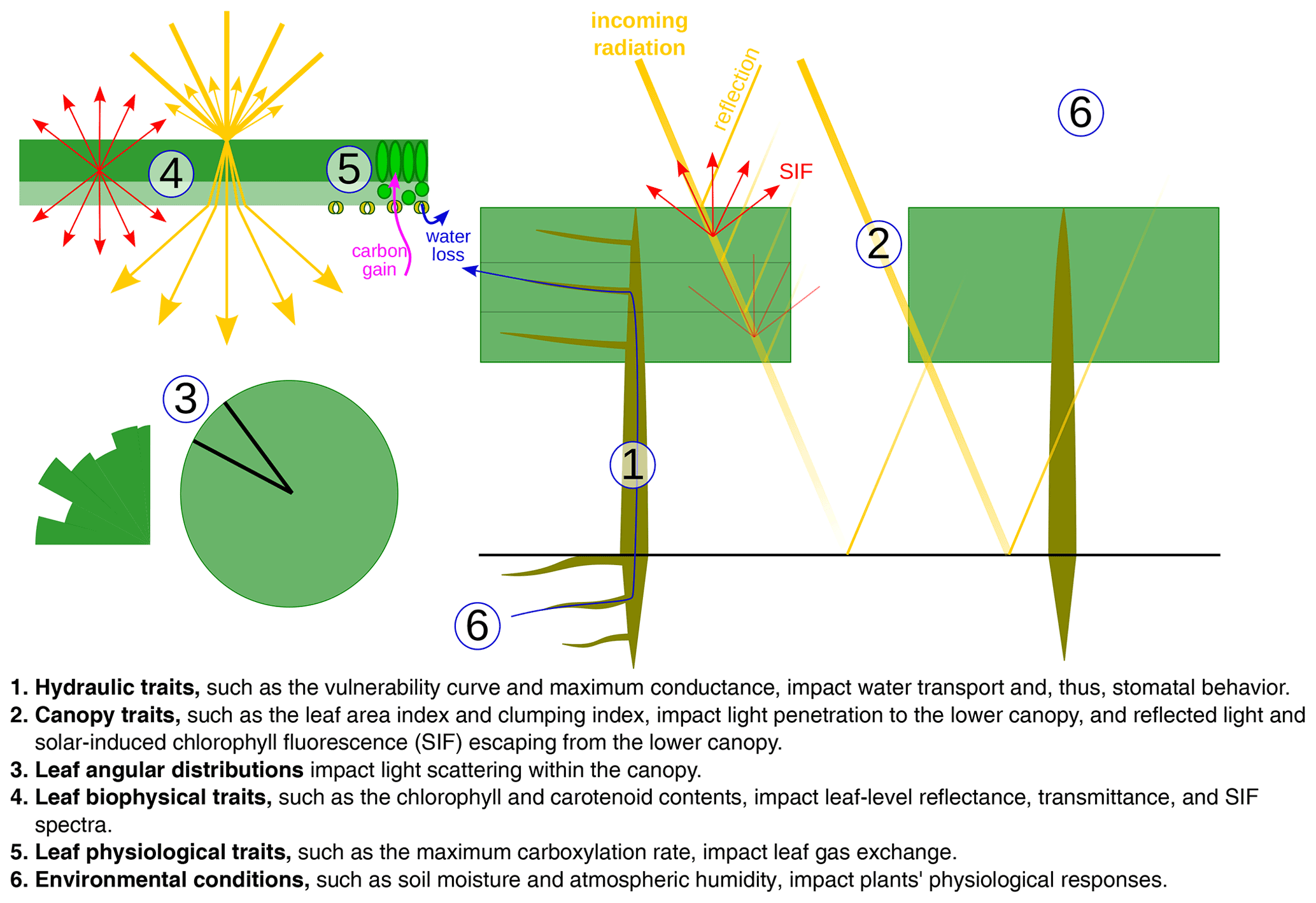
Figure 1Diagram of the CliMA Land model. CliMA Land is built on a highly modularized plant hydraulics module (labeled using 1). The plant hydraulic system has multiple roots, each tapping water in the corresponding soil layer; an optional trunk that elevates the plant canopy; and multiple branches, each connected to the corresponding canopy layer. The radiative transfer module within the canopy (labeled using 2) is responsible for simulating canopy-level light scattering by accounting for leaf angular distributions (labeled using 3) and leaf-level hyperspectral reflectance, transmittance, and fluorescence spectra (labeled using 4). The stomatal control module determines stomatal opening at the leaf level by assessing the photosynthetic and hydraulic status of the plant (labeled using 5) as well as environmental conditions (labeled using 6).
2.1 Plant architecture
In CliMA Land (v0.1), we treated a site as a uniform “mono-species” stand. Therefore, a suite of average plant traits were applied to the stand, and the stand-level simulation was done using these bulk traits. CliMA Land simulates plant hydraulics numerically using the most comprehensive and modular plant hydraulic system to date. The average plant was represented as a tree, and the modeled tree consisted of a multilayer root system, a trunk, and a multilayer canopy to match the soil and canopy setups (Fig. 2a). Each root layer corresponds to a horizontal soil layer, and contains a rhizosphere component and a root xylem in series (water flows through the rhizosphere and then the root xylem). All root layers are in parallel and connected to the base of the trunk. Each canopy layer corresponds to a horizontal air layer, containing a stem and leaves in series (water flows through the stem and then the leaves). All canopy layers are in parallel and connected to the top of the trunk. By default, we accounted for gravity in root and stem (gravity not accounted for in leaves); thus, each canopy layer has its own gravitational pressure drop. However, the gravity correction can be customized by setting the height changes of each root and stem. We note here that the hydraulic architecture in CliMA Land can be freely customized from a single xylem organ to a whole plant with any finite number of root and canopy layers. We assumed a uniformly distributed leaf area in the canopy, both vertically and horizontally, with the leaf orientation being evenly distributed in the azimuth. At each canopy layer and azimuth angle, we further adopted an angular distribution for the leaf inclination. By default, the leaf inclination angle is evenly distributed from 0 to 90∘. The inclusion of the leaf area fraction and leaf angle distribution allows us to simulate the bidirectional radiation within the canopy.

Figure 2The hydraulic system is customized to match the canopy layers to the canopy radiation model. (a) An example of a hydraulic system with multiple root layers, a trunk, and multiple canopy layers. (b) An example of a xylem water pressure profile in the hydraulic system when the soil water potential is −0.2 MPa for all soil layers. For better visualization, we use three root layers and three canopy layers in this example and compute the bulk mean leaf xylem pressure for all the leaves in each canopy layer. We account for the gravitational pressure drop in the root and stem (not in leaves) in the example; however, the gravitational pressure drop can be customized by setting the height change of each root and stem. We note here that there is an extraxylary component downstream of the leaf xylem. However, as the extraxylary flow does not impact xylem hydraulic conductance, it has little impact on the stomatal models that we use in our model. Nevertheless, the extraxylary component impacts the leaf water potential at the evaporation site and the leaf water content, and one needs to be cautious if the stomatal models are formulated using these physiology parameters.
We did not attempt to model the detailed hydraulic architecture within each root or canopy layer; thus, all transpiration within a root or canopy layer was transported via a single root or stem. All leaves in each canopy layer are in parallel and are connected to the end of the stem. The hydraulic flow and pressure profile were simulated for each leaf in each canopy layer. We simulated the flow and pressure at steady state; therefore, the following criteria were met: the total transpiration rate in each canopy layer was equal to the flow rate in the stem of that layer; the total flow rate of all canopy layers was equal to the flow rate in the trunk and the total flow rate of all root layers; and the root xylem pressure at the end of each root xylem was the same (namely, the pressure at the tree base; Fig. 2b).
We used constant leaf physiological parameters (such as hydraulic and photosynthetic traits) throughout the canopy, i.e., there was no difference between leaves with different azimuth or inclination angles. However, as we modeled the light environment for leaves at different layers and with different azimuth and inclination angles, we allowed the leaves to have different stomatal conductances and, thus, different photosynthetic rates. We note that our modeling framework allowed us to customize the vertical leaf area distribution, the leaf angular distribution, and the photosynthetic capacity profile vertically. Future research efforts to resolve these distributions within the canopy would make LSMs more realistic in terms of the upscaling of carbon, water, and energy fluxes. However, for now, we used even distributions in our model simulations due to the lack of knowledge on the true distributions at the study sites.
2.2 Canopy radiative transfer
We used the SCOPE model RT framework (Yang et al., 2017) to simulate the light environment within the canopy. However, we made some modifications to make the model more realistic. The first difference was that we accounted for carotenoid light absorption as part of absorbed photosynthetically active radiation (APAR; Frank and Cogdell, 1996; Kodis et al., 2004; Koyama et al., 2004). In brief, the relative absorption that is counted as APAR in SCOPE and CliMA Land (kAPAR,SCOPE and kAPAR,CliMA, respectively) differs as follows:
where αi is the feature absorption coefficient of the trace ingredient (cab for chlorophyll a + b, car for carotenoid), Ci is the content of each ingredient, and ∑(αiCi) is the sum of all ingredients (chlorophyll, violaxanthin and zeaxanthin carotenoid, brown pigment, anthocyanin, water, and dry mass). When accounting for carotenoids, APAR-related absorption relative to the total pigment absorption increases in the wavelength range from 400 to 550 nm (Fig. 3a). Thus, APAR increases for all leaves in each canopy layer because of the carotenoid absorption (an example is given in Fig. 3b). This extra light absorption by carotenoid drives increases in both SIF and gross primary productivity. As a result, our modeled photosynthetic rate and fluorescence ought to be higher than the original SCOPE model for the same model setup.
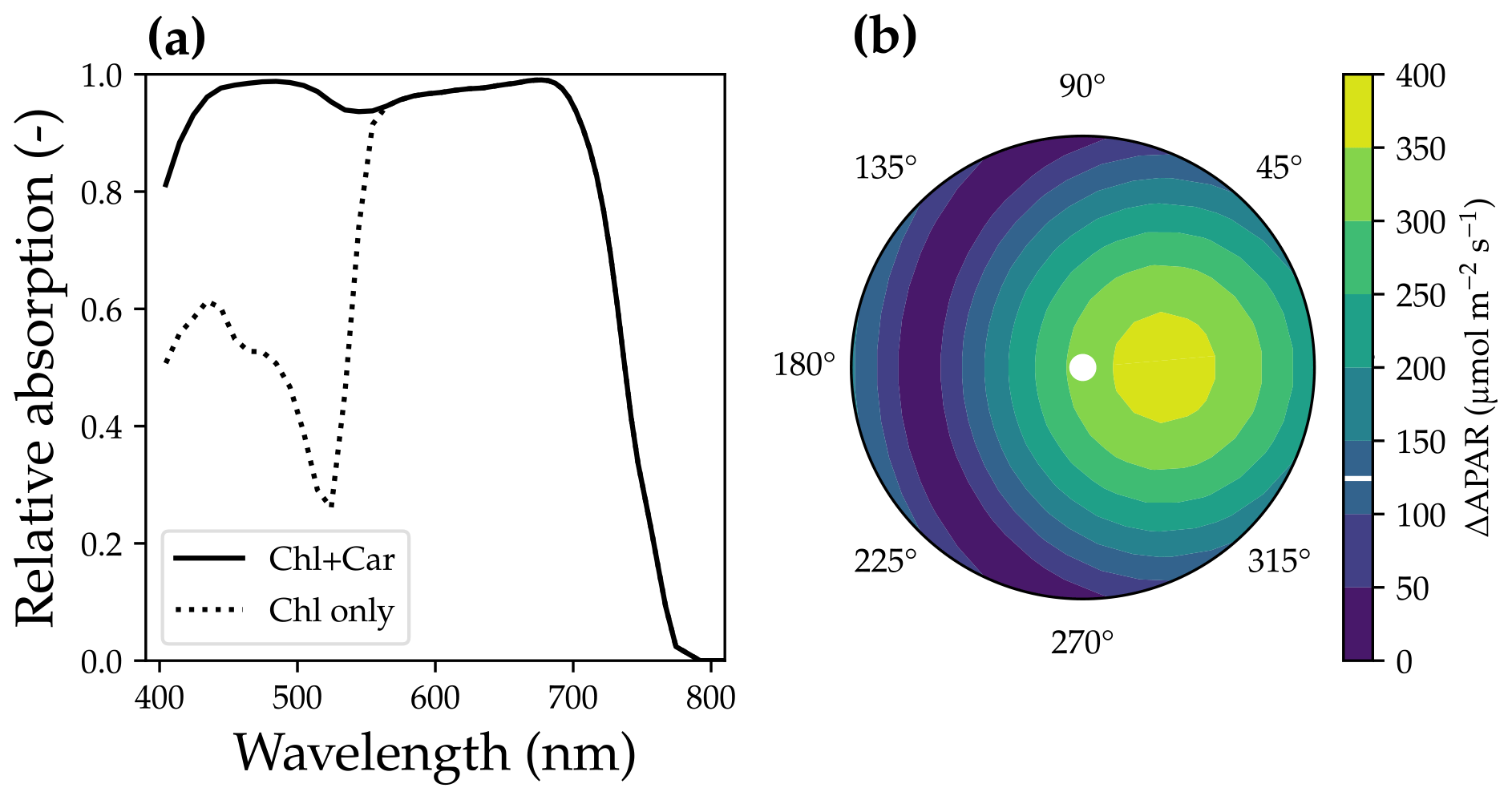
Figure 3The impact of carotenoid light absorption on absorbed photosynthetically active radiation (APAR). (a) The fraction of APAR light absorption relative to all pigment absorption. The solid curve represents the scenario when both chlorophyll and carotenoid absorption are counted as APAR. The dashed curve plots the scenario when only chlorophyll absorption is counted as APAR. (b) The APAR difference between the two scenarios for leaves with different azimuth angles (0 to 360∘) and inclination angles (axial direction, from 0 to 90∘). The colors indicate the increase in APAR for sunlit leaves with different angles when counting carotenoid absorption as APAR. The white line on the color bar indicates the increase in APAR for shaded leaves. The results are from the top canopy layer out of 20 layers for a canopy with a leaf area index of 3, a clumping index of 1, and a solar zenith angle of 30∘.
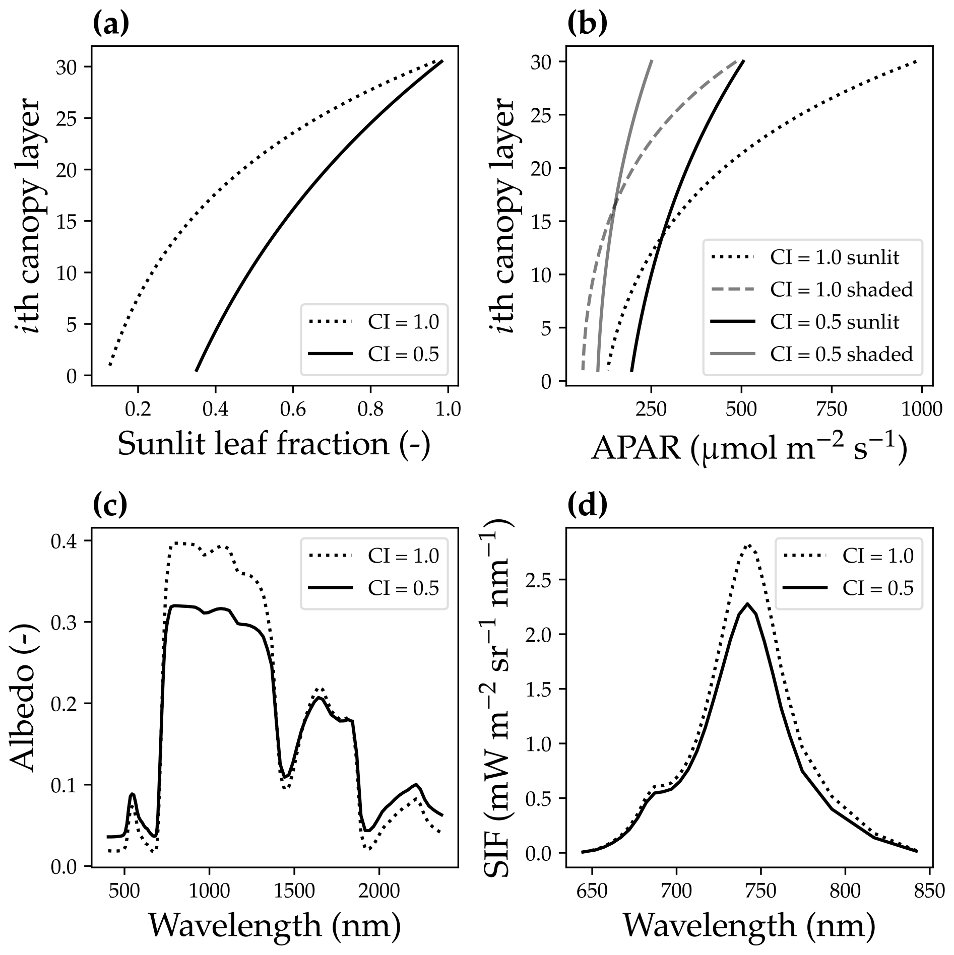
Figure 4The impact of canopy clumping on canopy radiative transfer. (a) The impact of the canopy clumping index (CI) on the sunlit leaf fraction. (b) CI impacts on the mean sunlit and shaded leaf-absorbed photosynthetic radiation (APAR). (c) CI impacts on the canopy reflectance spectrum. (d) CI impacts on the solar-induced chlorophyll fluorescence spectrum. The model simulation was done using a canopy with a leaf area index of 3, 30 canopy layers, a solar zenith angle of 30∘, a viewing zenith angle of 0∘, and a constant fluorescence yield of 1 %.
The second difference was that we accounted for the bidirectional reflectance distribution function effect of the canopy horizontal structure by incorporating a clumping index (CI; Braghiere et al., 2021). As the CI impacts the effective leaf area index (eLAI for effective value, and LAI for the true value) of an open canopy (Pinty et al., 2006; Braghiere et al., 2019, 2020), , we used eLAI in our model, whereas the original SCOPE model used LAI. When CI = 1, leaves are uniformly distributed in the horizontal; when CI < 1, there are gaps between and within clusters of leaves for each tree. The inclusion of a CI < 1 under low-soil-albedo values (we used a constant soil albedo of 0.2 in our model) results in a higher sunlit leaf fraction for every canopy layer, lower APAR for upper canopy layers, higher APAR for lower canopy layers, a different reflectance spectrum, and lower SIF (Fig. 4).
In the model simulations, we (1) calibrated the leaf chlorophyll fluorescence, reflectance, and transmittance spectra using the Fluspect-B model (Vilfan et al., 2016), which advances the PROSPECT model by computing the fluorescence matrices (Jacquemoud and Baret, 1990; Jacquemoud et al., 2009); (2) computed canopy optical properties (extinction coefficients for direct and diffuse light) from leaf inclination and azimuth distribution functions and sun-sensor geometry (Yang et al., 2017); (3) computed scattering coefficient matrices for direct and diffuse light based on the extinction coefficients and leaf reflectance and transmission spectra; (4) simulated the shortwave radiation through the canopy; (5) computed a variety of integrated fluxes, such as absorbed soil radiation and direct and diffuse APAR per layer (including angles for direct light); (6) calculated the steady-state stomatal conductance based on different stomatal models for each leaf angle, and then the fluorescence quantum yield from leaf photosynthesis; and (7) computed the four-stream radiation transport for SIF. We note here that as we include carotenoid absorption as APAR, leaf forward and backward fluorescence conversion matrices calculated using FLUSPECT-B model differ from those in SCOPE; however, leaf reflectance and transmittance spectra are the same as in SCOPE.
In the model, we represented a leaf azimuth angle from 0 to 360∘ at 10∘ increment steps (Nazim=36) and leaf inclination angle from 0 to 90∘ at 10∘ increment steps (Nincl=9). At each time step, we were able to calculate the fraction of sunlit leaf (fazim,incl) and APAR for each leaf angle combination (azimuth and inclination; e.g., Fig. 4). Therefore, we had a total of APAR values in each canopy layer (1 for the shaded leaf fraction), and the probability of each APAR value per layer was
where pazim,incl,n is the fraction of the sunlit part for the “azim”th azimuth angle and “incl”th inclination angle at the “n”th canopy layer (Nlay layers in total), and pshade,n is the fraction of the shaded part in the “n”th layer. Also, we had canopy reflectance and fluorescence spectra from a prescribed observation angle, from which we calculated SIF at 740 nm (SIF740).
2.3 Stomatal models
We used one optimization-based (Wang et al., 2020) and two empirical stomatal models (Ball et al., 1987; Medlyn et al., 2011) along with our modified version of the SCOPE RT scheme. For the optimization-based stomatal model (OSM), we calculated the steady-state stomatal conductance per leaf per canopy layer by maximizing the difference between the leaf-level carbon gain (represented by the net photosynthetic rate modeled using the classic Farquhar et al., 1980, model for C3 plants, Anet in ) and a risk (represented via leaf hydraulics and photosynthesis):
where E is the leaf-level transpiration rate (in ), and Ecrit is the critical transpiration rate for that leaf (in ), beyond which the leaf hydraulic conductance drops to 0.1 % of the maximum value (0.05 % in Sperry and Love, 2015; Sperry et al., 2016). Note that with the ascent of sap along the xylem, xylem water pressure becomes more negative (Fig. 2b), and the xylem hydraulic conductance decreases as a result of cavitation (Sperry and Tyree, 1988). The higher the leaf transpiration rate, the more negative the leaf xylem pressure is at the end of the leaf xylem in order to match transpiration and resupply of water to the leaf from the root system. However, leaf transpiration rate cannot be infinitely high because of xylem cavitation at negative xylem pressures. For example, for a leaf with a given xylem pressure at the leaf base (Ψbase), E peaks while leaf xylem pressure gets more and more negative (Fig. 5a), and E higher than this peak is physically unreachable.
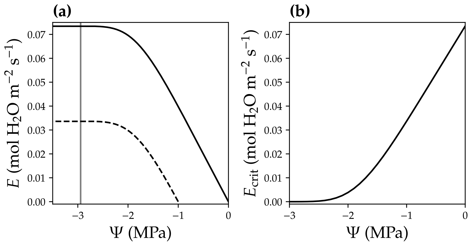
Figure 5Leaf critical flow rate changes with leaf base xylem pressure. (a) Leaf xylem water supply curves at two different leaf base xylem pressures (Ψbase; black solid curve for a Ψbase = 0 MPa, and black dashed curve for a Ψbase = −1 MPa). A xylem water supply curve is the plot of the leaf xylem flow rate (E) vs. leaf xylem end pressure (Ψ) at a given Ψbase (Ψ=Ψbase when E = 0). The gray vertical line plots the xylem pressure at which leaf xylem conductance reaches 0.1 % of the maximum. The intersection of the gray line and the xylem water supply curve indicates the critical xylem flow rate (Ecrit). (b) Ecrit decreases with more negative Ψbase.
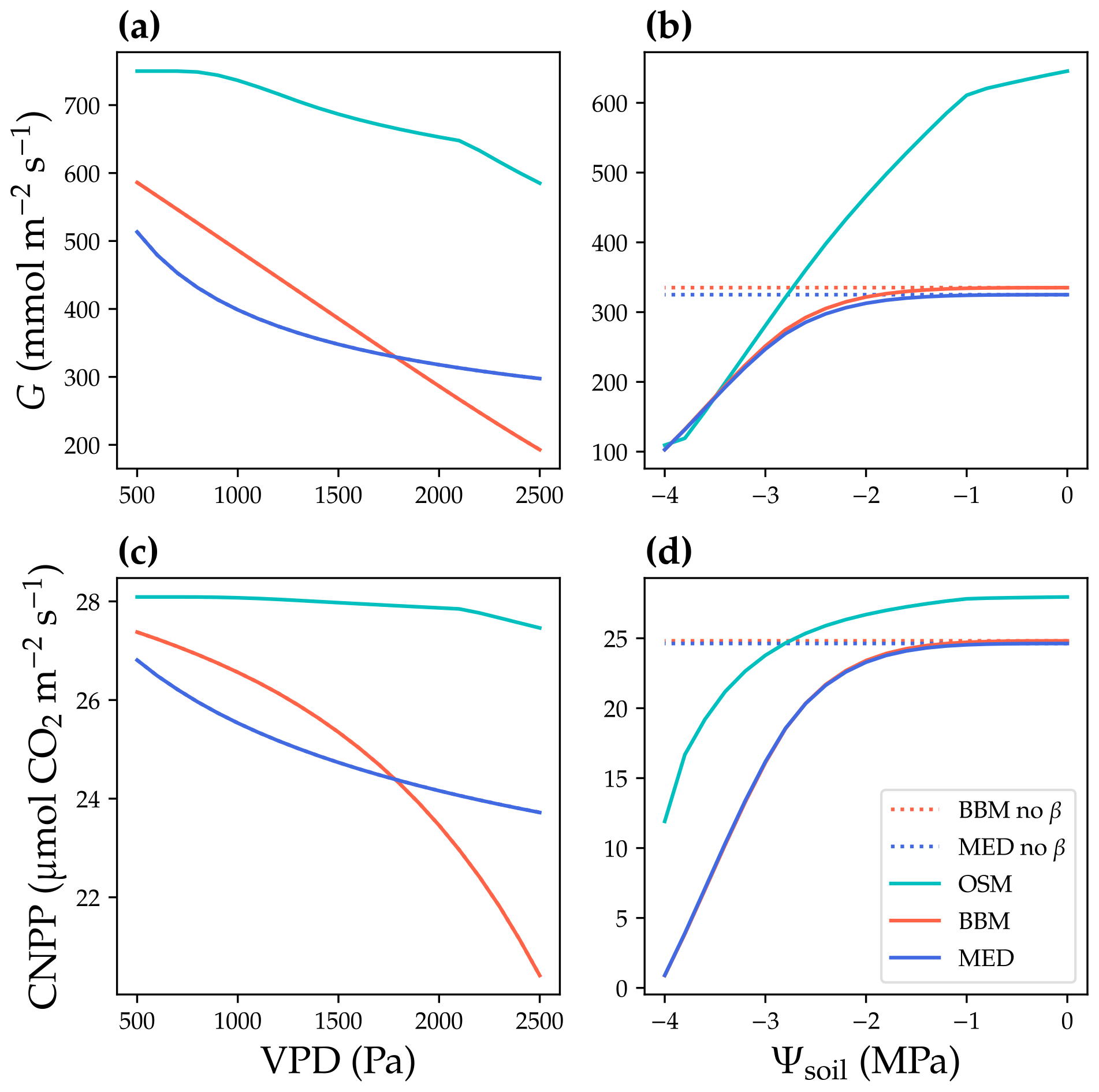
Figure 6Responses to environmental cues of three stomatal models. The stomatal models are the Ball et al. (1987), Medlyn et al. (2011), and Wang et al. (2020) stomatal model predictions (BBM, MED, and OSM, respectively). (a) Canopy cumulative stomatal conductance per ground area (G) response to the atmospheric vapor pressure deficit (VPD). The red and blue dotted lines plot the responses of the BBM and MED models without a tuning factor (β) for photosynthetic capacity, respectively. The red and blue solid lines plot the response of the BBM and MED models with a tuning factor for photosynthetic capacity (Eq. 8), respectively. The cyan solid line plots the response of the OSM model. The turning point around VPD = 1400 Pa is because leaf stomatal conductance hits the maximum structural limitation (0.2 in the example). (b) G responses to soil water potential (Ψsoil). (c–d) Canopy net primary productivity per ground area (CNPP, total canopy net photosynthetic rate per ground area, gross primary productivity minus canopy leaf respiration) responses to the VPD and Ψsoil.
We defined the transpiration rate at which the leaf xylem hydraulic conductance decreases to 0.1 % of the maximum value as Ecrit in our model (namely at 99.9 % loss of hydraulic conductance; Fig. 5a). We used a hybrid Bisection–Newton method algorithm provided by ConstrainedRootSolvers.jl (https://github.com/Yujie-W/ConstrainedRootSolvers.jl; last access: 13 April 2021) to numerically compute Ecrit (through solving the intersection of the gray line and xylem water supply curve in Fig. 5a). Ecrit decreases when Ψbase becomes more negative (Fig. 5; e.g., as a result of drier soil). The use of Ecrit in the risk function (Eq. 5) allowed us to predict the stomatal response to soil drought, as lower Ecrit resulted higher risk. See Fig. 6 for the theoretical whole-plant responses to the environmental stimuli for the OSM. Note that the risk term in Eq. (5) has the same mathematical form as Eq. (11a) in Wang et al. (2020), but the two differ in that Eq. (5) employs leaf-level flow rates for use with our adapted SCOPE RT model, whereas Eq. (11a) in the Wang et al. (2020) model employs mean canopy flow rates for use with the two-leaf radiation model. Therefore, Ecrit in CliMA Land differs among canopy layers given the different gravitational pressure drop and xylem pressure profiles.
For the Ball et al. (1987) stomatal model (BBM), we calculated the steady-state stomatal conductance (gsw in ) using an empirical formulation:
where RH is the relative humidity of the air (fraction; unitless), Cs is the leaf surface CO2 concentration (in µmol mol−1; after accounting for leaf boundary layer conductance as a function of wind speed), g0 (in ) and g1 (unitless) are fitting parameters for BBM, and βw is an empirical tuning factor that impacts leaf photosynthetic capacity and, thus, Anet. For the Medlyn et al. (2011) model (MED), the formulation reads
where D is the leaf-to-air vapor pressure deficit (in kPa), Ca is the atmospheric CO2 concentration (in µmol mol−1), and g0 (in ) and g1 (in ) are fitting parameters for MED. Note that these empirical stomatal models (BBM and MED) do not respond to soil moisture. To account for the soil moisture response, we followed the Community Land Model Version 5 (CLM5) approach by attenuating photosynthetic capacity via a stress factor (βw; Kennedy et al., 2019):
where K is the leaf hydraulic conductance calculated using the leaf xylem pressure, and Kmax is the maximal leaf hydraulic conductance. The use of a tuning factor helps address the stomatal response to soil moisture for BBM and MED. Note here that the tuning factor is applied per leaf per canopy layer. See Fig. 6 for the theoretical whole-plant responses to environmental stimuli for BBM and MED. As the BBM and MED models were used with a tuning factor on leaf photosynthetic capacity (represented by maximal carboxylation rate and maximal electron transport rate at a reference temperature, Vcmax25, and Jmax25 at 25 ∘C, respectively), the effective Vcmax25 used to compute photosynthetic rate was lower in the BBM and MED models compared with the OSM (when the three models used the same input). As a result, the BBM and MED model-predicted stomatal conductance and photosynthetic rate should be lower than the OSM (when the same model input was used; Fig. 6a, c). Furthermore, if the models are fitted to the same dataset, the BBM and MED tend to have higher fitted Vcmax25 to compensate for the negative effect from the tuning factor. The three models also differed in their sensitivity to soil moisture, as the penalty for the OSM increased with transpiration rate, whereas Vcmax25 would not be downregulated at relatively wet soil (e.g., soil water potential > −1 MPa; Fig. 6b, d).
For each of the three stomatal models (BBM, MED, and OSM), with the steady-state stomatal conductance for each APAR value, we computed the corresponding leaf net photosynthetic rate using the classic C3 photosynthesis model (Farquhar et al., 1980). The whole-canopy net primary productivity (CNPP, at an instant time) can then be computed using
3.1 Study sites
We used data from two flux tower sites to test the CliMA Land model. The first study site is located in a subalpine forest of the Niwot Ridge AmeriFlux core site (US-NR1) in the Rocky Mountains in Colorado, USA (40.03∘ N, 105.55∘ W; 3050 ; Fig. 7). The US-NR1 flux tower is surrounded by three dominate evergreen gymnosperm species: Abies lasiocarpa, Picea engelmannii, and Pinus contorta (Monson et al., 2002). The second study site is located in a broadleaf forest of the Missouri Ozark AmeriFlux site (US-MOz, MOFLUX) in Missouri, USA (38.74∘ N, 92.20∘ W; 219 ; Fig. 7). The US-MOz flux tower site is dominated by a deciduous angiosperm white oak (Quercus alba) mixed with several other deciduous species, including sugar maple (Acer saccharum) and hickory (Carya spp.) (Yang et al., 2007; Wood et al., 2019). See Tables 1 and 2 for details on the US-NR1 and US-MOz sites and the values used as model input. Hereafter, we refer the two sites as the gymnosperm site (US-NR1) and the angiosperm site (US-MOz).
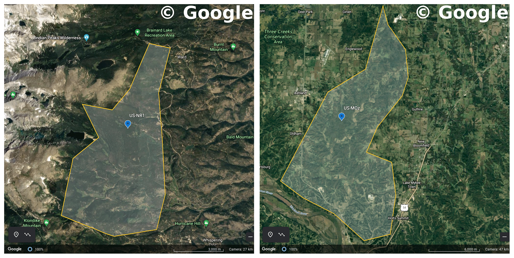
Figure 7Regions chosen to filter TROPOMI SIF observations. The left panel shows a Google Earth map for the US-NR1 flux tower site (Niwot Ridge, Colorado, USA). The right panel shows a Google Earth map for the US-MOz flux tower site (Ozark, Missouri, USA). The blue symbols show the flux tower locations, and the shaded regions are representative of area around the flux tower site. Map data were sourced from ©Google Earth Landsat/Copernicus.
Table 1Site and plant information of the Niwot Ridge flux tower site.
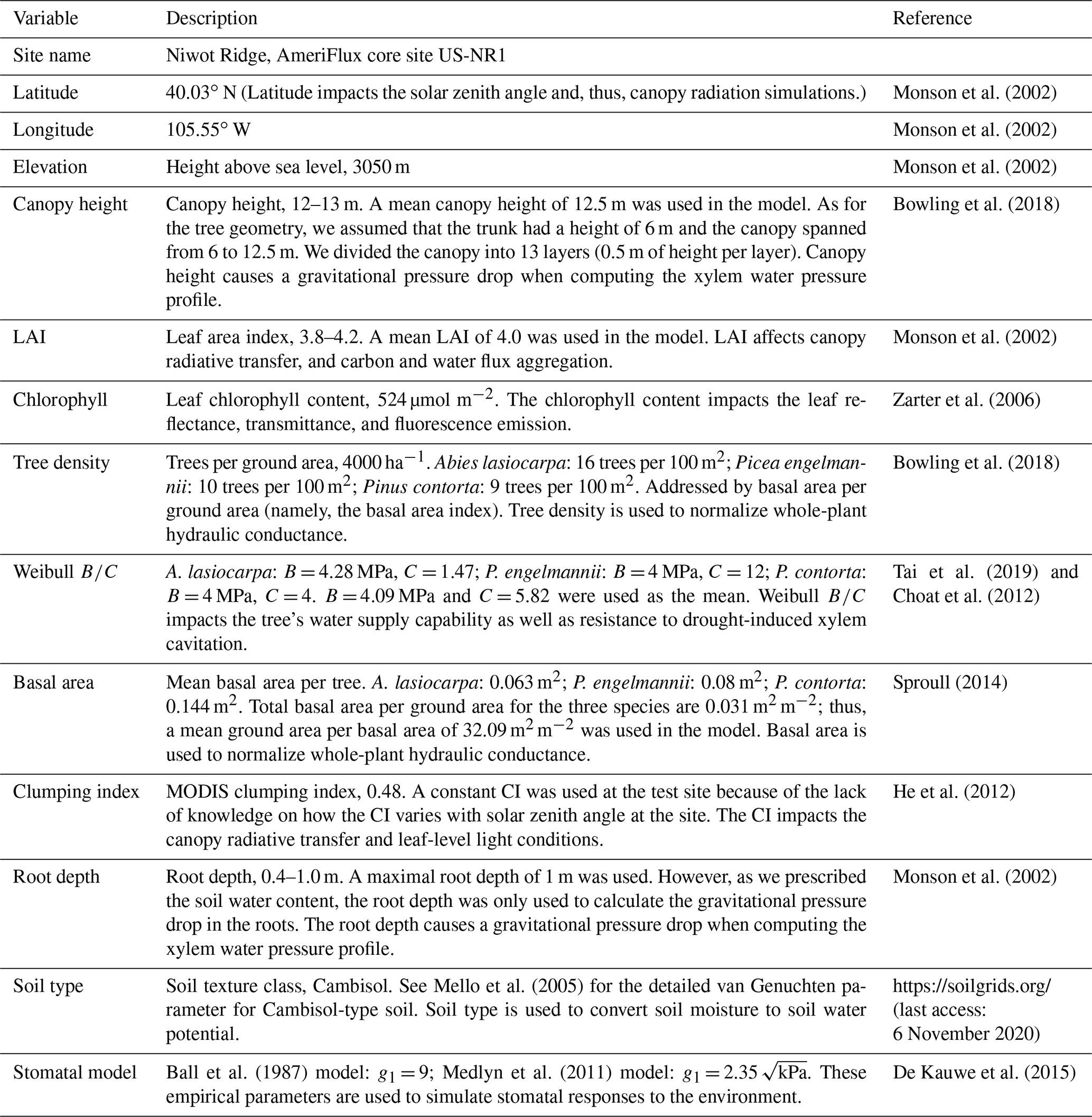
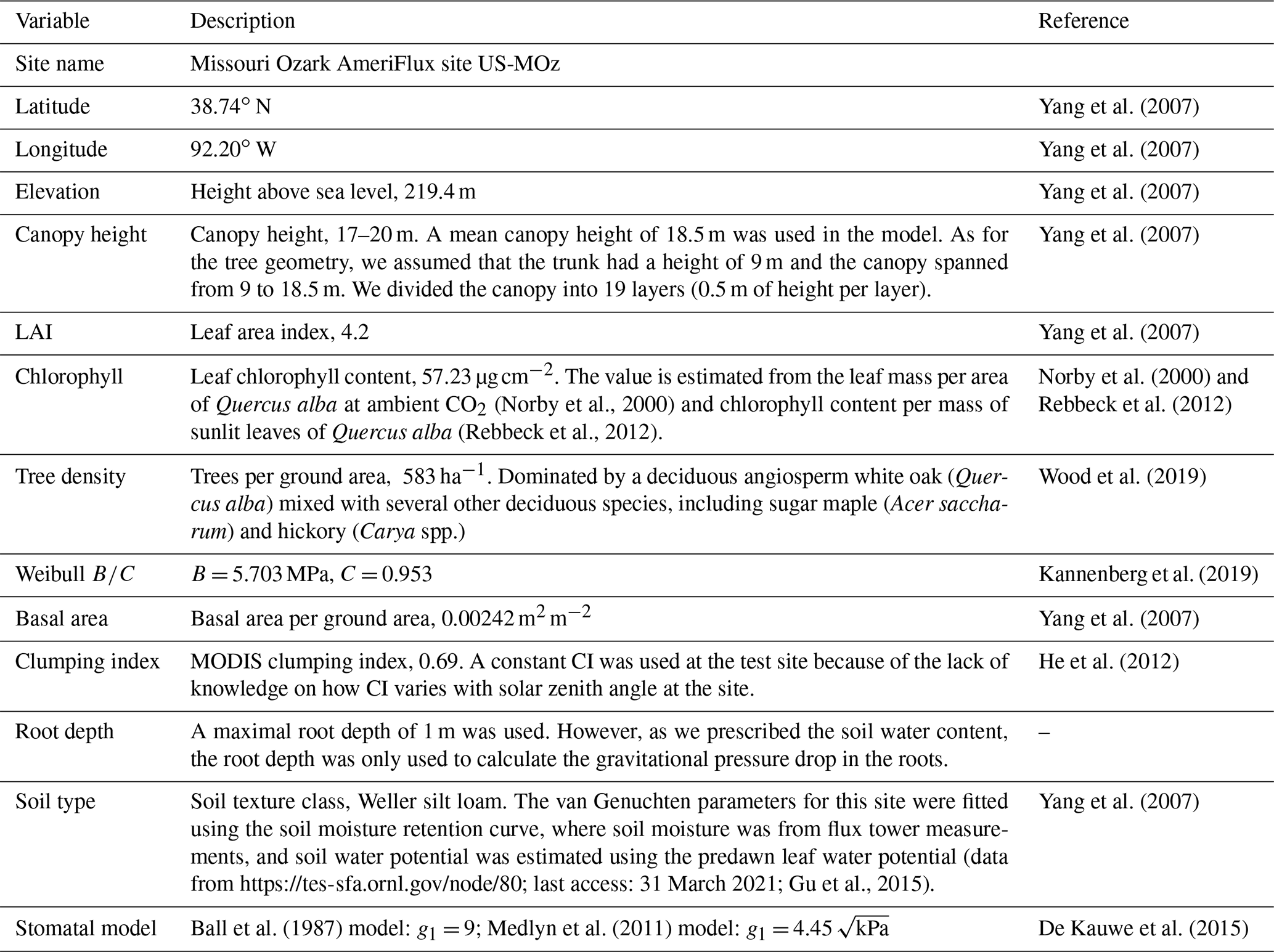
Table 2Site and plant information of the Missouri Ozark flux tower site (MOFLUX). See Table 1 for how each parameter is used in the model.
3.2 Model simulations
The flux tower sites have half-hourly mean flux estimates, as well as environmental conditions since 1998 (US-NR1) and 2004 (US-MOz). We chose the data from 2006 to 2019 to test our model due to the higher data quality (we omitted the year 2020 because the data were not yet available). We tested our model on an annual basis by splitting the original dataset into subsets (14 subsets for US-NR1, and 12 subsets for US-MOz due to missing data in 2006 and 2011). For each year, at each half-hour time step, we simulated the steady-state stomatal conductance and fluxes for the three stomatal models. To reduce uncertainty, we prescribed soil moisture, leaf temperature, and reported constant leaf area index (more details on the values we used can be found in Tables 1 and 2); we then ran offline simulations (namely, carbon, water, and energy fluxes do not feedback to the environmental conditions). We inverted leaf temperature using
where LWout is the surface-emitted longwave radiation from the flux tower measurement, ϵ is the emissivity of the leaf (0.97 following Campbell and Norman, 1998), σ is the Stefan–Boltzmann constant (5.67 × 10⁻⁸ W K−4), and Tleaf is the mean leaf temperature (in K).
To further reduce the uncertainty in the evaluation of flux tower data when comparing model simulations to observations, we compared the modeled carbon and water fluxes directly to flux tower estimations rather than reprocessed products such as gross primary productivity (GPP). Thus, we did not perform the typical step that partitions observed net ecosystem exchange of CO2 (NEE) into GPP and ecosystem respiration. Instead, we partitioned the ecosystem to canopy and non-canopy parts. We simulated NEE as the difference between the canopy net exchange (namely CNPP) and the remaining respiration (wood and soil, represented by Rremain): . In this way, the daytime canopy net photosynthetic rate and nighttime respiration rate were used as CNPP, whereas the remaining respiration of wood and soil was computed as a function of soil temperature (Tsoil):
where Rbase is the respiration normalized to a reference temperature (298.15 K in our model), f(Tsoil) is the temperature correction, and Q10 is the exponent used for temperature correction (1.4 for angiosperm and 1.7 for a gymnosperm plant following Lavigne and Ryan, 1997).
At each time step, we (1) calculated the soil water potential and leaf temperature from the flux tower measurements; (2) computed the solar zenith angle based on the site latitude and local time; (3) simulated the canopy radiative transfer, and obtained APAR values for sunlit and shaded leaves in each canopy layer; (4) updated environmental conditions and leaf temperature per canopy layer; (5) computed the steady-state stomatal conductance for each leaf angle in each canopy layer using the classic C3 photosynthesis model (Farquhar et al., 1980), and summed the canopy carbon and water fluxes of the entire canopy; (6) modeled leaf-level fluorescence yield using the computed steady-state photosynthetic rate with van der Tol et al. (2014) model parameters and modeled site-level SIF740 with the updated version of the SCOPE model; (7) calculated Rremain from soil temperature using Eq. (11); and (8) compared site-level modeled NEE and water fluxes (ET) to flux tower estimates. For the hydraulic system, we assumed that the xylem hydraulic conductance recovered when the soil rehydrated (in other words, we did not model the drought legacy effect within or across growing seasons).
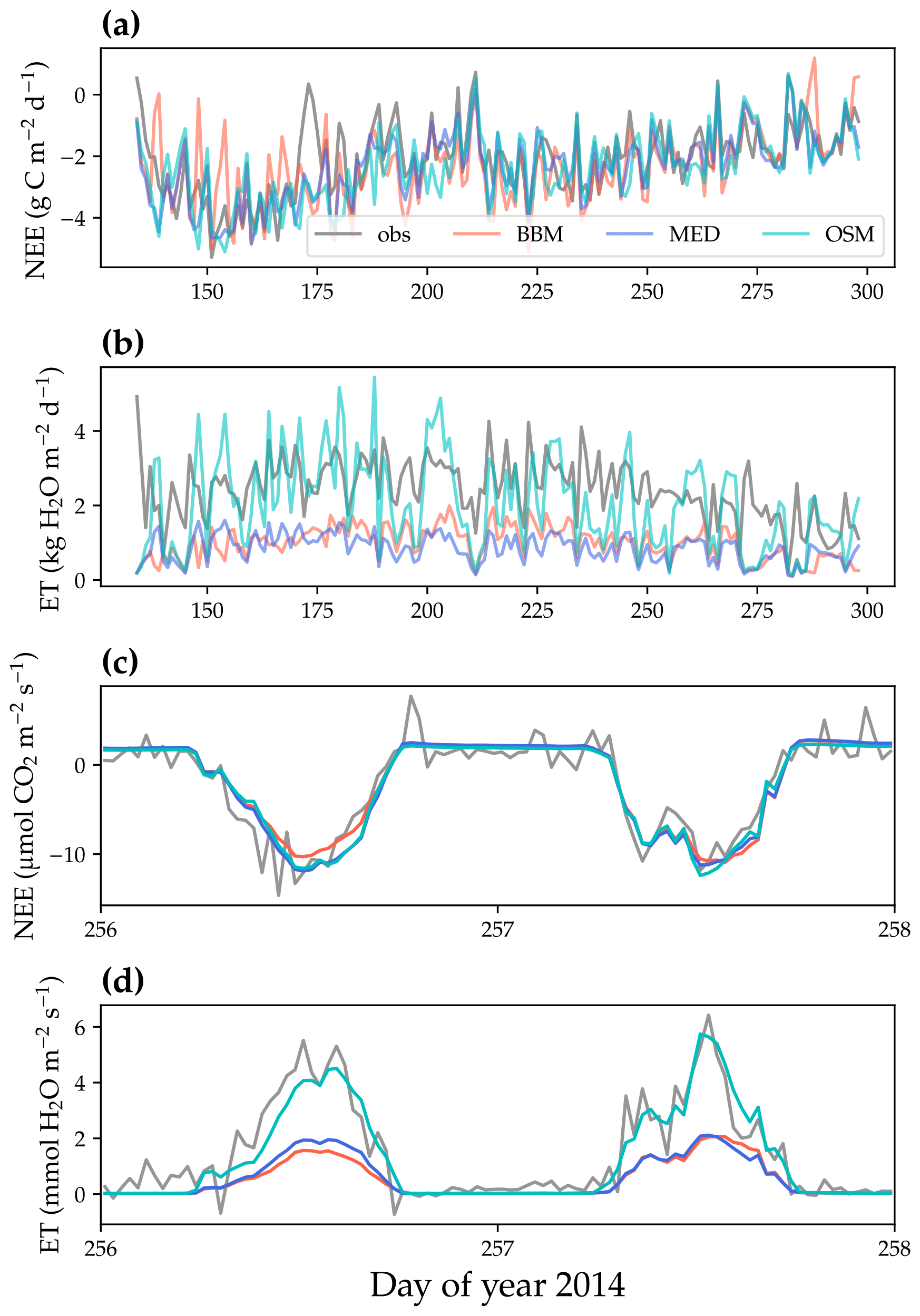
Figure 8Comparison of model-predicted carbon/water fluxes to the US-NR1 (Niwot Ridge, evergreen gymnosperm forest) flux tower – observations for the year 2014. (a) The gray curve plots the daily CO2 flux in the growing season. The shaded red, blue, and cyan curves plot the respective Ball et al. (1987), Medlyn et al. (2011), and Wang et al. (2020) stomatal model predictions (BBM, MED, and OSM, respectively). (b) Comparison of modeled and observed daily total transpiration flux. (c) Comparison of half-hourly modeled and observed net ecosystem carbon flux (NEE) for days 256–257 of the year 2014. (d) Comparison of modeled and observed ecosystem water flux (ET) for days 256–257 of the year 2014.
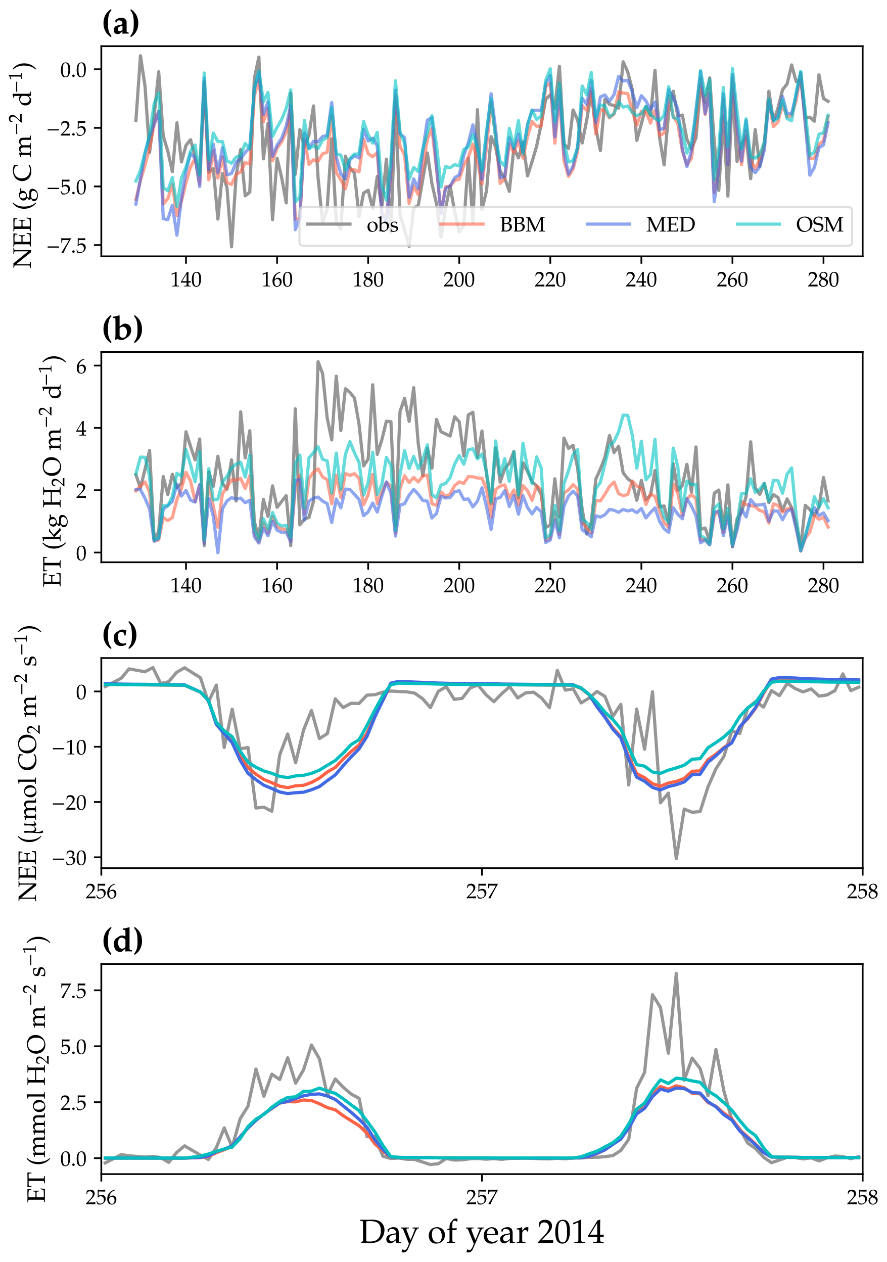
Figure 9Comparison of model-predicted carbon/water fluxes to the US-MOz (MOFLUX, deciduous angiosperm forest) flux tower – observations for the year 2014. (a) The gray curve plots the daily CO2 flux in the growing season. The shaded red, blue, and cyan curves plot the respective Ball et al. (1987), Medlyn et al. (2011), and Wang et al. (2020) stomatal model predictions (BBM, MED, and OSM, respectively). (b) Comparison of modeled and observed daily total transpiration flux. (c) Comparison of half-hourly modeled and observed net ecosystem carbon flux (NEE) for days 256–257 of the year 2014. (d) Comparison of modeled and observed ecosystem water flux (ET) for days 256–257 of the year 2014.
Note that there were some missing essential parameters in our model: site-level bulk photosynthetic capacity (namely, Vcmax25 and Jmax25), hydraulic conductance per basal area (namely, Kmax), and Rbase. These parameters have a large impact on model simulations, as Vcmax25, Jmax25, and Kmax affect stomatal opening (and, thus, canopy carbon and water fluxes), and Rbase affects stand carbon flux. We note that there were some Vcmax25 and Jmax25 observations for US-MOz for a few years (Gu et al., 2015), but a complete time series of Vcmax25 and Jmax25 was not available. Therefore, we fitted these parameters by minimizing the mean absolute standardized error of both carbon and water fluxes for each year:
where the subscripts “mod” and “obs” represent model and observation, respectively, and “mean” and “SD” are functions to compute mean value and standard deviation, respectively. Note that we fitted Vcmax25 (), Kmax (we assumed a constant root : stem : leaf resistance ratio of , consistent with the ratio used by Sperry et al., 2017), and Rbase for each stomatal model to make a fair comparison of the three models. We only used the flux data from the growing season of each year, and the growing season period was defined as the time when the mean daily carbon flux was higher than 1 for 7 consecutive days. Note that a constant Vcmax25 was used for all three models rather than a time series. However, because of the model setup, the OSM used a constant Vcmax25 throughout the growing season, whereas the BBM and MED used a variable effective Vcmax25 as a result of the tuning factor to account for the stomatal response to soil moisture. The reader is referred to Figs. 8 and 9 for examples of the fitted results for the gymnosperm and angiosperm forests, respectively.
3.3 Model performance
All three stomatal models (one optimization-based and two empirical models) were able to track the diurnal and seasonal carbon and water fluxes (e.g., Fig. 8 for the gymnosperm site and Fig. 9 for the angiosperm site). In general, all three models quantitatively predicted the net ecosystem carbon flux (Figs. 8a and c, 9a and c, 10, and 11). However, predicted water fluxes diverged across the models, as the BBM and MED models tended to underestimate water fluxes, and the OSM model better matched the magnitude of water flux (Figs. 8b and d and 9b and d). The reader is referred to Figs. S1–S26 in the Supplement for the comparison of the time series of carbon and water fluxes for each site in each growing season.
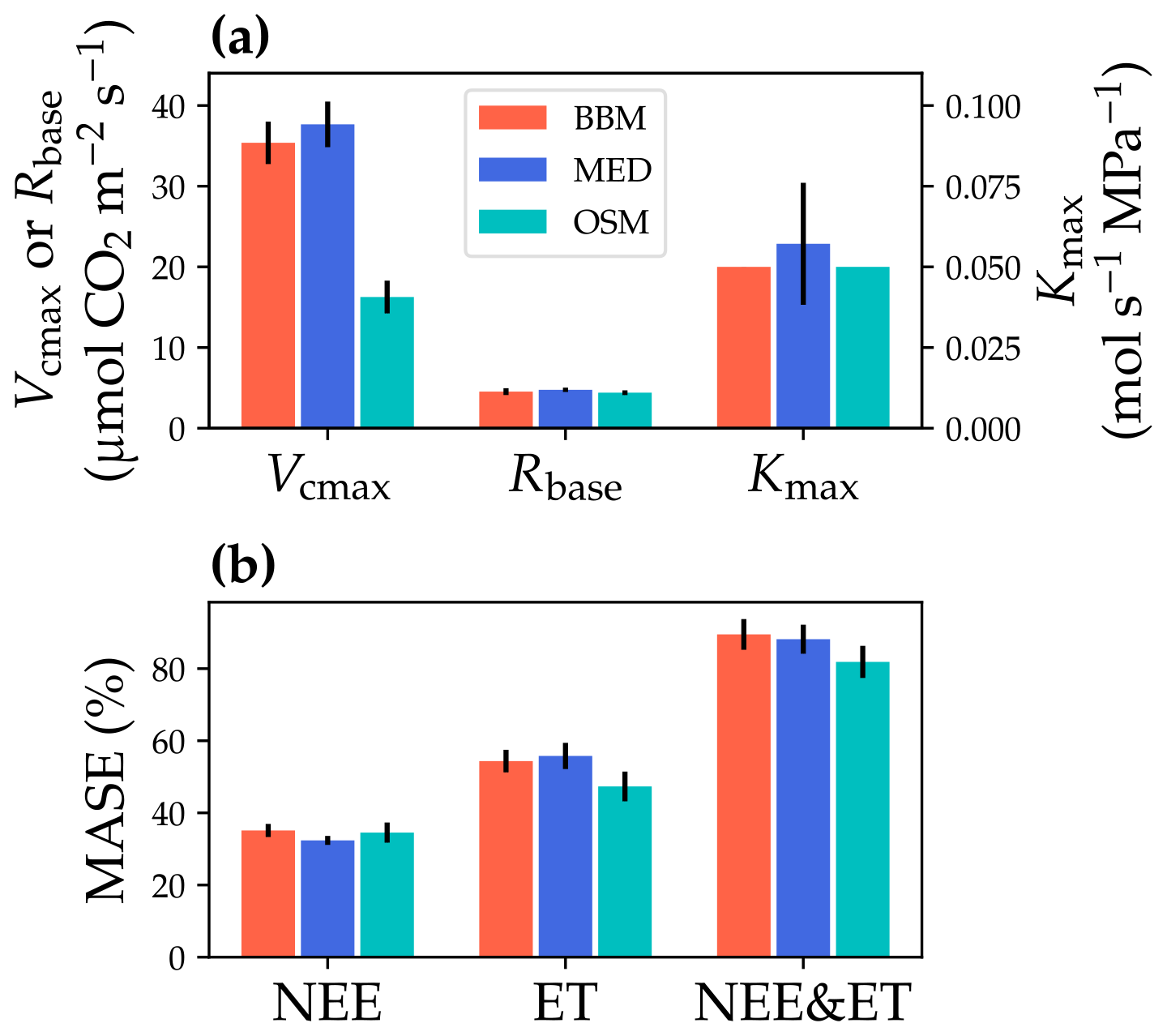
Figure 10Comparisons of the fitted model parameters and model predictive skills for the US-NR1 (Niwot Ridge, evergreen gymnosperm forest) flux tower. (a) The red bars plot the mean of the fitted parameters for the Ball et al. (1987) stomatal model (BBM). The fitting parameters are the maximal carboxylation rate at 25 ∘C (Vcmax25), the soil respiration rate at 25 ∘C (Rbase), and the maximal whole-plant hydraulic conductance (Kmax). The blue and cyan bars plot the means for the Medlyn et al. (2011) (MED) and Wang et al. (2020) (OSM) models, respectively. Black error bars plot the standard deviation of the fitting parameter. (b) Comparison of mean absolute standardized error (MASE, Eq. 12) for the carbon flux (NEE), water flux (ET), and both NEE and ET.
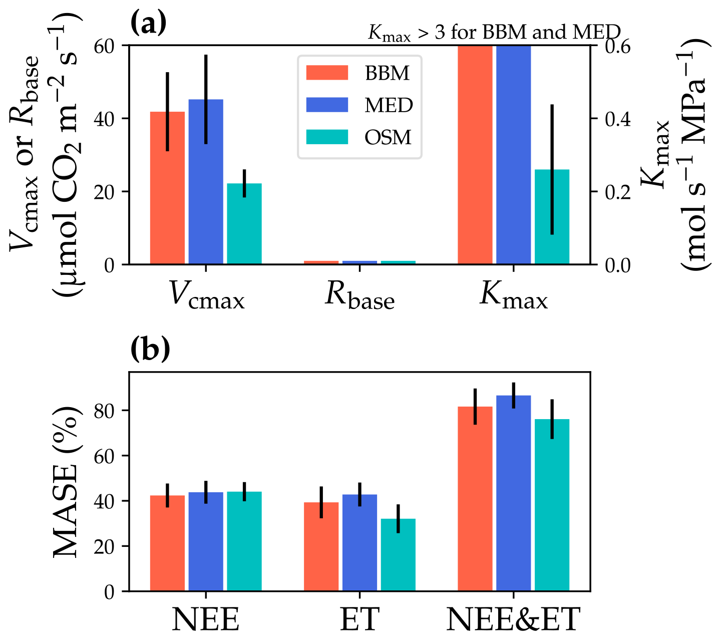
Figure 11Comparisons of the fitted model parameters and model predictive skills for the US-MOz (MOFLUX, deciduous angiosperm forest) flux tower. (a) The red bars plot the mean of the fitted parameters for the Ball et al. (1987) stomatal model (BBM). The fitting parameters are the maximal carboxylation rate at 25 ∘C (Vcmax25), the soil respiration rate at 25 ∘C (Rbase), and the maximal whole-plant hydraulic conductance (Kmax). The blue and cyan bars plot the means for the Medlyn et al. (2011) (MED) and Wang et al. (2020) (OSM) models, respectively. Black error bars plot the standard deviation of the fitting parameter. The fitted Kmax of the BBM and MED reaches the maximum limit of the Kmax ranges (4 ) and is way higher than that of the OSM; thus, the bars are cut off for comparison with the OSM. (b) Comparison of mean absolute standardized error (MASE, Eq. 12) for the carbon flux (NEE), water flux (ET), and both NEE and ET.
3.3.1 Fitting parameter variation
The same variables, Vcmax25, Rbase, and Kmax, were fitted for all three stomatal models. In terms of fitting parameter variation, the OSM generally had the lowest standard deviation, whereas BBM and MED generally had a higher standard deviation (Figs. 10a, 11a; Table 3). In terms of MASE, the OSM had the lowest error (sum of both carbon and water fluxes), whereas the BBM and MED had a higher error (Figs. 10b, 11b; Table 4).
Table 3Fitting parameters of the three stomatal models: the Ball et al. (1987) model (BBM), the Medlyn et al. (2011) model (MED), and the Wang et al. (2020) model (OSM). Numbers shown in the table are the mean ± standard deviation. The fitted parameters include the following: the maximum carboxylation rate at 25 ∘C (Vcmax25), root respiration at 25 ∘C (Rbase), the maximal tree hydraulic conductance per basal area (Kmax), and the empirical stomatal parameter g1 (unitless for BBM, in for MED).
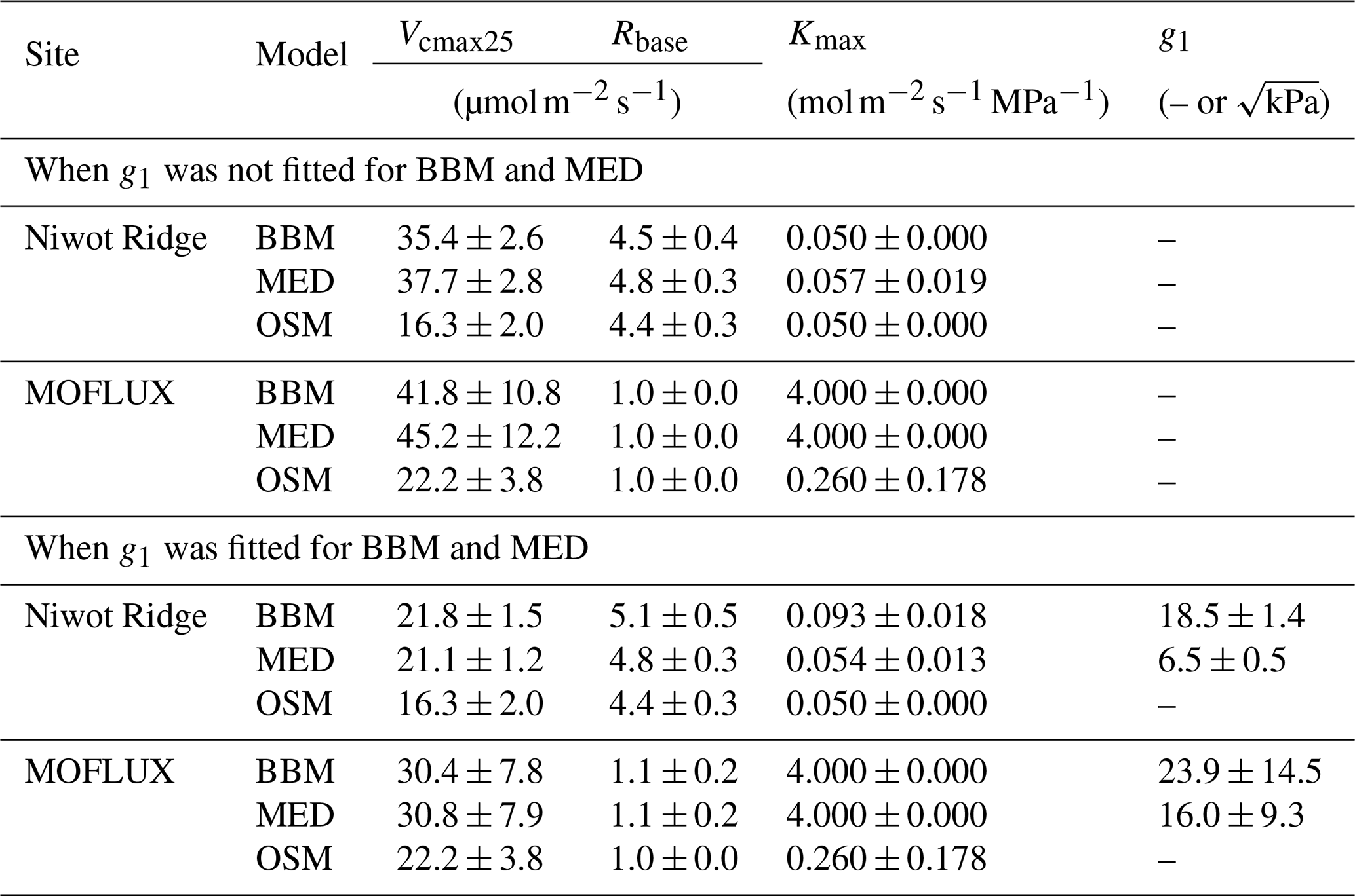
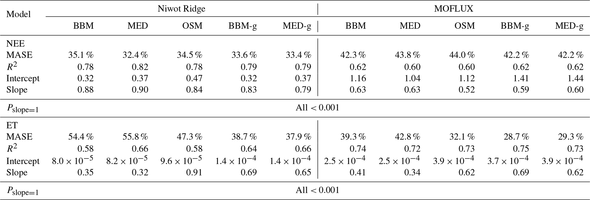
Table 4Statistics of the three stomatal models' predictive skills. The models are the Ball et al. (1987) model (BBM), the Medlyn et al. (2011) model (MED), and the Wang et al. (2020) model (OSM). The NEE section shows the regression details of the modeled vs. observed net ecosystem carbon flux (NEE), whereas the ET section shows the regression details of the modeled vs. observed ecosystem water flux (ET). The MASE row shows the mean absolute standardized error (mean for each year). The Pslope=1 row indicates the P value for which the slope is not different from one. The BBM-g and MED-g columns display the results when an extra empirical parameter “g1” (Eqs. 6, 7) is also fitted for the empirical model.
While all three stomatal models had similar fitted soil respiration (Rbase), the models had divergent fitted photosynthetic capacity (Vcmax25) and maximal hydraulic conductance (Kmax). In general, the empirical models required higher Vcmax25 (Figs. 10a, 11a). The reason for this is that the empirical models in the present study were used along with a tuning factor for effective Vcmax25 (Kennedy et al., 2019). In comparison, the stomatal optimization model weighs the carbon gain and risk trade-off to determine stomatal opening, and effective Vcmax25 is held constant throughout the simulation. Thus, for empirical models, leaf-level effective Vcmax25 is always lower than the fitted value because of the negative leaf xylem pressure. Given that the fitted parameters were bulk properties of the sites, we expected them to differ from leaf-level observations but be of the same magnitude. However, because of the limited direct measurements in the studied forest sites, we were only able to find one study reporting a Vcmax25 that ranged from 8 to 12 and a Jmax25 that ranged from 46 to 57 at Niwot Ridge (Tomaszewski and Sievering, 2007). Therefore, the OSM-estimated Vcmax25 = 15 seemed to be reasonable, and as we explained, the BBM- and MED-estimated Vcmax25 values had to be higher than the OSM estimate due to the tuning factor.
We note that varying the effective Vcmax25 based on leaf hydraulic conductance loss is only one form of the ad hoc tuning factor to force stomatal responses to drought (e.g., see Powell et al., 2013, Trugman et al., 2018, and Kennedy et al., 2019, for alternative formulations). The advantage of a Vcmax25 tuning factor is that it helps account for the decreasing effective Vcmax25 during drought (either due to a real drop in photosynthetic capacity or mesophyll conductance; Dewar et al., 2018) and, thus, could be more realistic in water-limited scenarios; however, tuning the effective Vcmax25 for short-term changes in leaf water potential may harm the model performance (such as diurnal changes of leaf water potential when there is no soil drought; Wang et al., 2020). In comparison, the OSM used a constant Vcmax25 throughout a growing season, and it would not be able to capture the decrease in Vcmax25 if it happens. Despite the fact that Vcmax25 does decrease during drought (e.g., Zhou et al., 2014, 2016), there is no direct evidence that Vcmax25 varies linearly with leaf water potential, plant/leaf hydraulic conductance, soil moisture, or soil water potential for all species. A better understanding of how Vcmax25 varies during and after a drought will improve the accuracy of modeling carbon and water fluxes for all stomatal models.
The fitted Kmax was comparable for all three models at the gymnosperm site, but it was much higher for empirical models at the angiosperm site. The reason for this contrasting behavior was also the tuning factor based on hydraulic conductivity loss. The xylem vulnerability curve in our model was represented by a Weibull function: , where B indicates the xylem pressure at ca. 63 % loss of conductivity, and C indicates the steepness of the decrease in k. Although the tested angiosperm forest had a higher B = 5.70 MPa compared with 4.09 MPa for the gymnosperm forest, C = 0.95 of the angiosperm site was much lower than that of gymnosperm site (5.82). As a result, the effective Vcmax25 used in the BBM and MED models dropped dramatically at relatively lower negative soil water potential for the angiosperm site (e.g., > −2 MPa), while the effective Vcmax25 barely changed for the gymnosperm site. At the default g1 setting, the empirical models underestimate water flux; thus, the optimized Kmax would be higher to increase the canopy water flux. However, we note that the error does not change much for very high Kmax because the water flux is mainly controlled by the g1 parameter in the empirical models.
3.3.2 Quantitative comparison
In terms of minimal under- or overestimation, the OSM showed the highest predictive skill because of its better performance with respect to predicting water fluxes. For the gymnosperm site, combining all data and simulations from 14 growing seasons from 2006 to 2019, we found that model-predicted carbon fluxes were generally near 1:1 compared to flux tower observations for all three models (Fig. 12a, b, c). However, the slopes of the linear regressions (red lines in Fig. 12a, b, c) for the carbon flux were all significantly lower than 1 (despite the fact that the slopes were close to 1; P<0.001; more detailed statistics are given in Table 4). As for the water flux, all three models underestimated water fluxes compared with the flux tower observations (Fig. 12d, e), and the slopes were all significantly lower than 1 (P<0.001; Table 4). The stomatal optimization model based on plant hydraulics (OSM), however, better predicted the water flux (Fig. 12f) compared with the empirical models. We found a similar pattern for the angiosperm site (Fig. 13; Table 4). In general, the model performances were slightly worse in MOFLUX, given the higher error in predicted NEE and the shallower slope for both the NEE and ET. The relatively worse performances were likely due to the higher variation in observed NEE and ET, e.g., many NEE observations were higher than 10 .
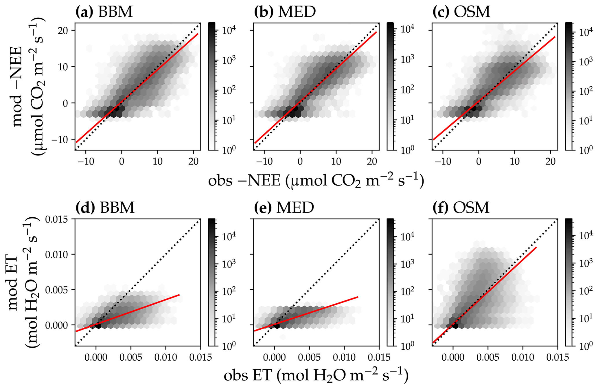
Figure 12Comparison of half-hourly modeled and observed carbon and water fluxes for the three stomatal models for the US-NR1 (Niwot Ridge, evergreen gymnosperm forest) flux tower. (a) Comparison of modeled (y axis) and observed (x axis) net ecosystem carbon flux (NEE) for the Ball et al. (1987) stomatal model (BBM). Shading represents density: the darker the hexagon, the more data that fell within the hexagon. The red solid line plots the linear regression of the data, and the black dotted line plots the 1:1 line. (b) Comparison of NEE for the Medlyn et al. (2011) model (MED). (c) Comparison of NEE for the Wang et al. (2020) model (OSM). (d) Comparison of ecosystem water flux (ET) for the BBM. (e) Comparison of ET for the MED. (f) Comparison of ET for the OSM.
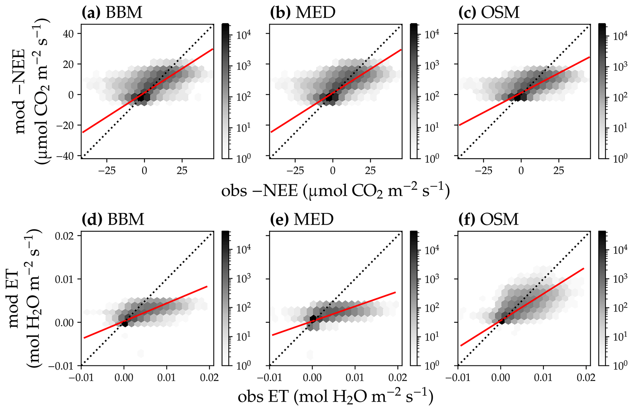
Figure 13Comparison of half-hourly modeled and observed carbon and water fluxes for the three stomatal models for the US-MOz (MOFLUX, deciduous angiosperm forest) flux tower. (a) Comparison of modeled (y axis) and observed (x axis) net ecosystem carbon flux (NEE) for the Ball et al. (1987) stomatal model (BBM). Shading represents density: the darker the hexagon, the more data that fell within the hexagon. The red solid line plots the linear regression of the data, and the black dotted line plots the 1:1 line. (b) Comparison of NEE for the Medlyn et al. (2011) model (MED). (c) Comparison of NEE for the Wang et al. (2020) model (OSM). (d) Comparison of ecosystem water flux (ET) for the BBM. (e) Comparison of ET for the MED. (f) Comparison of ET for the OSM.
Our model simulations suggest that implementing a plant hydraulic trait-based stomatal optimization model into vegetation models has great potential with respect to improving the model predictive skills, particularly for the water flux (Figs. 12, 13), adding new evidence to existing literature (e.g., Anderegg et al., 2018; Venturas et al., 2018; Wang et al., 2019; Eller et al., 2020; Sabot et al., 2020). Moreover, while the stomatal optimization model (Wang et al., 2020) had lower errors than the empirical models (Ball et al., 1987; Medlyn et al., 2011), the optimization model fitting parameters did not vary much (Figs. 10, 11). In comparison, the empirical models required more variable parameterization among years to achieve a similar error (Figs. 10a, 11a). Furthermore, as the stomatal optimization model did not rely on empirical parameters like g0 and g1, the stomatal optimization model can be used to simulate plant carbon and water fluxes with acclimated traits (Sperry et al., 2019). In comparison, it is unclear how g0 and g1 may vary with plant traits, adding extra uncertainties to modeling plant responses to future climate.
3.3.3 Land model parameterization
In general, the empirical models using default CLM setups did not perform as well as the stomatal optimization model. This underperformance may result from an imperfect land model parameterization that was adopted in our model simulations. For example, CLM uses a constant g1 for a plant functional type regardless of where the plant grows (in a wet or dry region); moreover, g1 is estimated using gas exchange measurements for well-watered plants and, thus, may not represent a drought stress scenario very well. Furthermore, the use of a Vcmax25 tuning factor interfered with the prescribed g1. For example, if the g1 was meant to be used with a tuning factor that affects g1 itself rather than Vcmax25, the use of g1 with a Vcmax25 tuning factor would make the model more sensitive to air humidity when the plant suffers from drought stress. The reason for this is that a Vcmax25 tuning factor would translate changes in leaf water potential into changes in effective Vcmax25, and stomatal conductance would then decrease faster in response to drier air. In this case, the prescribed g1 needs to be higher to mitigate the increased sensitivity resulting from the Vcmax25 tuning factor.
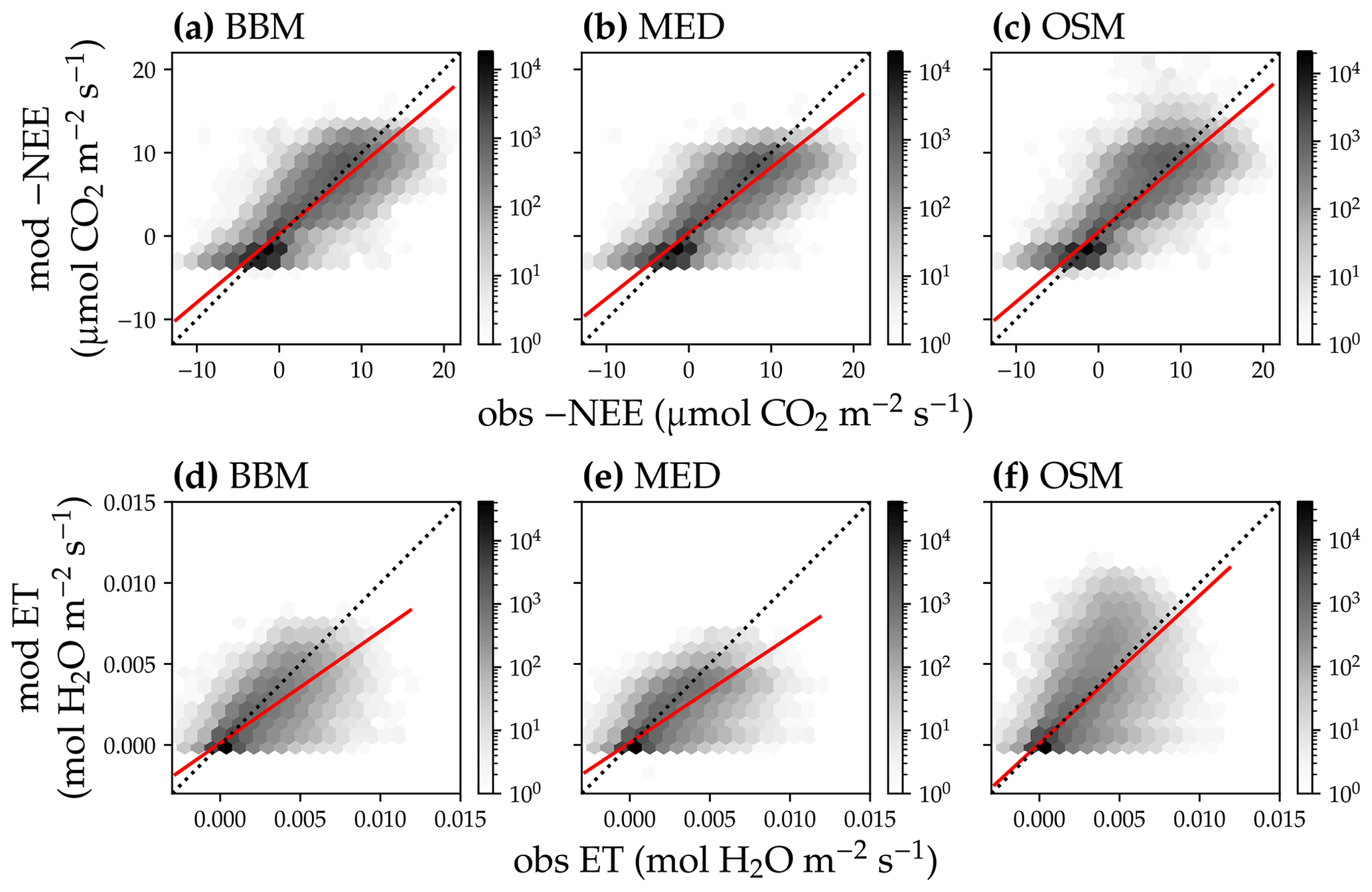
Figure 14Comparison of modeled and observed carbon and water fluxes for the three stomatal models when fitting an extra empirical model stomatal model parameter for the US-NR1 (Niwot Ridge, evergreen gymnosperm forest) flux tower site. (a) Comparison of modeled (y axis) and observed (x axis) net ecosystem carbon flux (NEE) for the Ball et al. (1987) stomatal model (BBM). Shading represents density: the darker the hexagon, the more data that fell within the hexagon. The red solid line plots the linear regression of the data, and the black dotted line plots the 1:1 line. (b) Comparison of NEE for the Medlyn et al. (2011) model (MED). (c) Comparison of NEE for the Wang et al. (2020) model (OSM). (d) Comparison of ecosystem water flux (ET) for BBM. (e) Comparison of ET for MED. (f) Comparison of ET for OSM. This figure differs from Fig. 12 in that g1s (Eqs. 6, 7) for BBM and MED are also fitted.
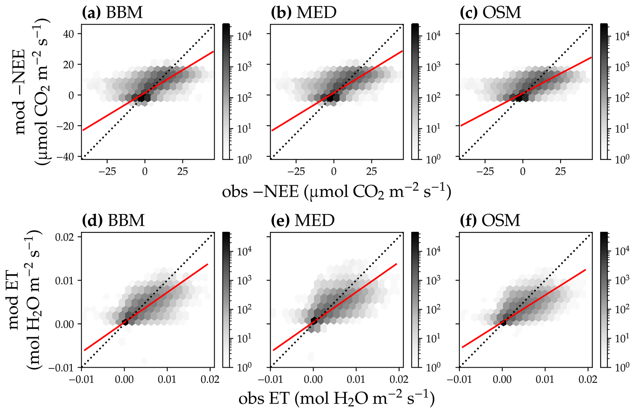
Figure 15Comparison of modeled and observed carbon and water fluxes for the three stomatal models when fitting an extra empirical model stomatal model parameter for the US-MOz (MOFLUX, deciduous angiosperm forest) flux tower site. (a) Comparison of modeled (y axis) and observed (x axis) net ecosystem carbon flux (NEE) for the Ball et al. (1987) stomatal model (BBM). Shading represents density: the darker the hexagon, the more data that fell within the hexagon. The red solid line plots the linear regression of the data, and the black dotted line plots the 1:1 line. (b) Comparison of NEE for the Medlyn et al. (2011) model (MED). (c) Comparison of NEE for the Wang et al. (2020) model (OSM). (d) Comparison of ecosystem water flux (ET) for BBM. (e) Comparison of ET for MED. (f) Comparison of ET for the OSM. This figure differs from Fig. 13 in that g1s (Eqs. 6, 7) for the BBM and MED are also fitted.
Indeed, when we fitted an extra g1 for both BBM and MED models, we found improved predictive skills in tracking water flux, as the slope between modeled and observed ET were closer to 1 (although still significantly lower than 1; Table 4; Figs. 14, 15). However, the increase in the slopes of ET was accompanied by decreases in the slopes of NEE (Table 4; Figs. 14, 15). As we expected, the fitted g1 was much higher than in the CLM5 default setups (Table 3). It is also worth noting that when g1 was fitted for the empirical stomatal models, our fitting g1 was higher than CLM defaults, and fitted Vcmax25 was also closer to the OSM (Table 3). The changes in the fitted Vcmax25 were likely due to the higher stomatal conductance caused by higher g1 (as the model-predicted water fluxes increased). For example, if the fitted Vcmax25 did not change when g1 was higher, the empirical models would predict higher stomatal conductance and, thus, a higher photosynthetic rate. In this case, the error between model-predicted carbon fluxes and flux tower observations would increase. As the BBM- and MED-predicted carbon flux was already centered along the 1:1 line vs. flux tower observations (as in Figs. 12a and b and 13a and b), an unchanged Vcmax25 would result in higher biases in the carbon flux, harming the overall empirical model performance. Therefore, the fitted Vcmax25 decreased, whereas g1 increased to minimize the error between model predictions and observations.
The alteration of g1 within the empirical models shows potential with respect to better capturing carbon and water fluxes than the tested stomatal optimization model (Table 4), and we believe that more site-specific g1 setups would improve the empirical model predictive skills. However, whether the fitted parameters also apply to other forests, and how to best represent the spatial and temporal variations in g1 require further investigation. Nevertheless, as g1 is supposed to change with time, empirical model-predicted future carbon and water fluxes may be very uncertain. In comparison, the OSM was less dependent on empirical curve-fitted parameters and had lower variation in the fitting parameters (Figs. 10, 11); thus, the model-predicted future carbon and water fluxes could be more reliable. Given the underperformance of empirical models when we used a different tuning factor algorithm (on photosynthetic capacity), we highlight the fact that (1) inverted model parameters for use in LSMs vary with the model used to fit these parameters, and (2) using parameters inverted from one model setup in another model would likely result in biases in model outputs.
Our model simulations highlighted the importance of land model parameterization as well as the potential pitfalls in using unpaired or untested parameter sets in land surface modeling. As such, we recommend revisiting and recalibrating the land model parameterization based on the stomatal model and tuning factor algorithm that was used for each LSM based on real measurements. Comparatively, the tested optimization model shows comparable predictive skills and is less dependent on the empirical parameters (better than the default CLM setups but worse than the scenario of fitting an extra g1). We also emphasize that using flux tower data to invert site-level bulk traits for use in stomatal optimization has great potential with respect to advancing future land surface modeling. We foresee how global flux tower data could be used to estimate the missing traits, particularly hydraulic traits. Furthermore, machine-learning-based algorithms along with climatological data would help solve the issue of sparsely distributed towers. Knowing how these traits vary globally not only helps global simulations using stomatal optimization theory but also provides a direct way to assess the status of plants' hydraulic health, thereby aiding in the prediction of zones that are at risk of drought-induced tree mortality and potentially shifting traits due to climate change. Better future land model parameterization ought to improve the land surface modeling and, thus, Earth system modeling.
4.1 Study sites
We used the TROPOMI SIF retrievals that fell within the region of the flux tower sites to test our model, excluding retrievals that had a cloud fraction higher than 10 % (see Fig. 7 for the region map). For the gymnosperm site, we chose retrievals that had at least 50 % overlap with a representative area around the flux tower site (a total of 99 data points in 2018 and 2019); for the angiosperm site, we chose retrievals that had at least an 80 % overlap with the representative site region (a total of 218 points in 2018 and 2019). For each valid TROPOMI SIF retrieval, we simulated the SIF emission using the actual sun-sensor geometry angles with our CliMA Land model (solar zenith angle, viewing zenith angle, and relative azimuth angle).
4.2 Model simulations
We first aligned the TROPOMI SIF retrievals with flux tower data (e.g., if the satellite observation occurred at 12:48 LT (local time), we aligned the data to a flux tower observation ranging from 12:30 to 13:00 LT). With the fitted Vcmax25, Kmax, and Rbase, we calculated the photosynthetic rate and fluorescence quantum yield at each time step (van der Tol et al., 2014). We then used the modeled quantum yield to simulate the canopy SIF spectrum for the given sun-sensor geometry. We modeled SIF at 740 nm for both the gymnosperm and angiosperm forests for 2018 and 2019, and compared our model-simulated SIF740 against TROPOMI SIF740. We simulated SIF in two scenarios: (i) a constant LAI (same prescribed value as the carbon and water flux simulations) was used to simulate SIF throughout the year, and (ii) a time series of LAI from the Moderate Resolution Imaging Spectroradiometer (MODIS) instrument was used (data from Yuan et al., 2011, with a spatial resolution of ∘ and a temporal resolution of 8 d).
4.3 Model performance
For both LAI scenarios (using constant site LAI or using variable MODIS LAI), the modeled SIF captured the trend of TROPOMI SIF retrievals well (Fig. 16; P < 0.001 for all four linear regressions). When using variable MODIS LAI, modeled SIF had better agreement with the SIF retrievals (lower root-mean-square error, RMSE, for both forests; Fig. 16). The statistically significant linear correlation between modeled and observed SIF suggests that satellite-based remote sensing data have potential with respect to constraining future land model parameterization.
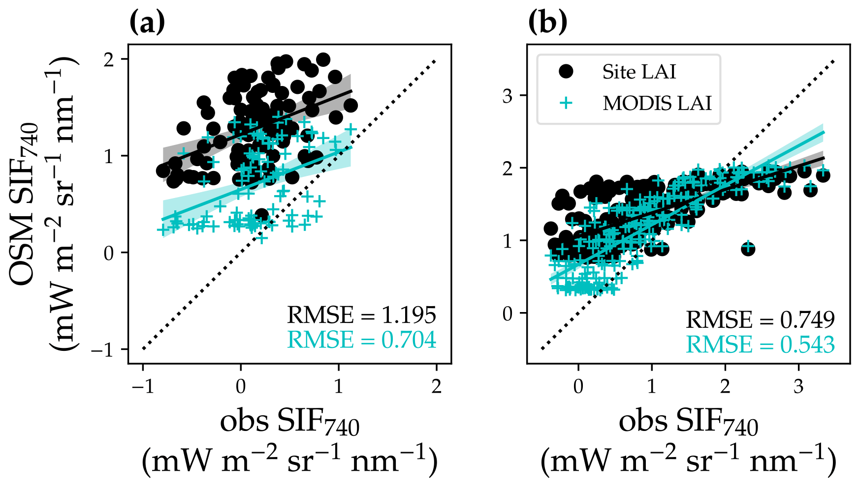
Figure 16Comparison of modeled and satellite-observed solar-induced chlorophyll fluorescence at 740 nm (SIF740). (a) Comparison for the US-NR1 flux tower site (evergreen gymnosperm forest). The black circles plot the comparison with modeled SIF using a constant site LAI, and the cyan “+” symbols plot the comparison using a variable MODIS LAI time series. The black line with shaded confidence interval regions plots the linear regression for the black circles (, R2=0.17, P<0.001). The cyan line with shaded regions plots the linear regression for the cyan symbols (, R2=0.14, P<0.001). (b) Comparison for the US-MOz flux tower site (deciduous angiosperm forest). The linear regressions are , R2=0.54, P<0.001 for the black circles and , R2=0.69, P<0.001 for the cyan symbols.
Our model captured the seasonal cycle of SIF compared to satellite observations, underscoring the potential to constrain land model parameterization using remote sensing products. However, we were not able to obtain a 1:1 relationship between modeled and retrieved SIF given the significant intercept (P< 0.001; Fig. 16). There are many potential reasons for the offset, e.g., retrieval noise (some TROPOMI SIF values were lower than zero), mismatches in the spatial and temporal domain, inaccurate parameters to model SIF (leaf biomass per area, leaf chlorophyll content, and seasonal changes in leaf area index), and high sustained non-photochemical quenching (NPQ) at Niwot Ridge due to low temperature (accounting for the sustained NPQ will make the modeled SIF lower in wintertime, namely the points with lower observed SIF; Porcar-Castell, 2011; Raczka et al., 2019). Despite all of these imperfections, we still found a strong correlation between modeled and satellite-based SIF. Furthermore, when we used an LAI time series (Yuan et al., 2011), the agreement between modeled and satellite-based SIF increased, which indicated the potential of constraining land model parameters using remote-sensing-based results. Future research with improved parameterization of our land model and more accurate plant and site traits would likely improve the model performance.
We implemented and tested a new land surface model that couples a comprehensive canopy radiative transfer scheme with a stomatal optimization model based on plant hydraulic traits, and two empirical stomatal models. We investigated how the three models performed at two flux tower sites (one dominated by gymnosperm species, and the other dominated by angiosperm species). We compared model-predicted carbon and water fluxes to flux tower estimations, and model-predicted SIF to satellite-based TROPOMI SIF retrievals. All three stomatal models performed well with respect to predicting site-level carbon fluxes, showing similar 1:1 correlations and errors among all three models. However, the stomatal optimization model showed better agreement with water flux observations, given the improved 1:1 comparison with the flux tower observations. In comparison, the empirical stomatal models underestimated water fluxes and had a higher error, probably due to the nonideal parameterization. Our model also reproduced the seasonal pattern of canopy SIF, with dynamic ranges most likely being different due to heterogeneity in the area around the tower. We concluded that the representation of the land model using the stomatal optimization theory along with a more comprehensive RT model have great potential with respect to predicting site-level carbon and water fluxes. Furthermore, the use of a comprehensive RT scheme allows us to quantitatively and directly link land surface processes to remote sensing, making it possible to constrain land model parameterization with a broad range of remote sensing datasets. The rapidly growing regional and global datasets will make it easier to better parameterize and evaluate land surface modeling and better predict the future carbon cycle and climate.
Flux tower datasets are freely available at AmeriFlux (registration required; US-NR1: https://doi.org/10.17190/AMF/1246088, Blanken et al., 2021; US-MOz: https://doi.org/10.17190/AMF/1246081, Wood and Gu, 2021). The gridded MODIS LAI is available at http://globalchange.bnu.edu.cn/research/laiv6 (Yuan et al., 2020, 2011) and has also been made available via “GriddingMachine.jl” (https://github.com/CliMA/GriddingMachine.jl, last access: 27 September 2021; https://doi.org/10.22002/D1.2129, Wang, 2021b). We refer the reader to the online documentation of “GriddingMachine.jl” for access to the datasets (along with other high-quality gridded datasets such as TROPOMI SIF). We coded our model and did the analysis using Julia (version 1.6.0), and the current version of the CliMA Land model is available from the project website (under the Apache 2.0 License): https://github.com/CliMA/Land (last access: 29 March 2021). The exact version of the model used to produce the results employed in this paper is archived on Zenodo (https://doi.org/10.5281/zenodo.4762775, Wang, 2021a), as are the input data and scripts to run the model and produce the plots for all the simulations presented (Wang, 2021a).
The supplement related to this article is available online at: https://doi.org/10.5194/gmd-14-6741-2021-supplement.
YW designed and conducted the research. YW, CF, and RKB developed the CliMA Land model. PK performed the TROPOMI SIF retrieval. YW, PK, LH, RD, RKB, JDW, and CF performed the general data analysis and wrote the paper.
The contact author has declared that neither they nor their co-authors have any competing interests.
Publisher's note: Copernicus Publications remains neutral with regard to jurisdictional claims in published maps and institutional affiliations.
We gratefully acknowledge the generous support of Eric and Wendy Schmidt (by recommendation of the Schmidt Futures) and the Heising-Simons Foundation. Part of this research was carried out at the Jet Propulsion Laboratory, California Institute of Technology, under a contract with the National Aeronautics and Space Administration (NASA).
This research has been supported by the NASA Earth Sciences Division (grant no. NNX15AH95G), the Schmidt Futures program, and the Heising-Simons Foundation.
This paper was edited by Christoph Müller and reviewed by two anonymous referees.
Anav, A., Friedlingstein, P., Kidston, M., Bopp, L., Ciais, P., Cox, P., Jones, C., Jung, M., Myneni, R., and Zhu, Z.: Evaluating the land and ocean components of the global carbon cycle in the CMIP5 earth system models, J. Climate, 26, 6801–6843, 2013. a
Anderegg, W. R., Wolf, A., Arango-Velez, A., Choat, B., Chmura, D. J., Jansen, S., Kolb, T., Li, S., Meinzer, F. C., Pita, P., de Dios, V. R., Sperry, J. S., Wolfe, B. T., and Pacala, S.: Woody plants optimise stomatal behaviour relative to hydraulic risk, Ecol. Lett., 21, 968–977, 2018. a, b
Arora, V. K., Boer, G. J., Friedlingstein, P., Eby, M., Jones, C. D., Christian, J. R., Bonan, G., Bopp, L., Brovkin, V., Cadule, P., Hajima, T., Ilyina, T. Lindsay, K., Tjiputra, J. F., and Wu, T.: Carbon–concentration and carbon–climate feedbacks in CMIP5 earth system models, J. Climate, 26, 5289–5314, 2013. a
Badgley, G., Anderegg, L. D., Berry, J. A., and Field, C. B.: Terrestrial gross primary production: Using NIRV to scale from site to globe, Glob. Change Biol., 25, 3731–3740, 2019. a
Baldocchi, D., Falge, E., Gu, L., Olson, R., Hollinger, D., Running, S., Anthoni, P., Bernhofer, C., Davis, K., Evans, R., Fuentes, J., Goldstein, A, Katul, G., Law, B., Lee, X., Malhi, Y., Meyers, T., Munger, W., Oechel, W., Paw U, K. T., Pilegaard, K., Schmid, H. P., Valentini, R., Verma, S., Vesala, T., Wilson, K., and Wofsy, S.: FLUXNET: A new tool to study the temporal and spatial variability of ecosystem-scale carbon dioxide, water vapor, and energy flux densities, Bulletin of the American Meteorological Society, 82, 2415–2434, 2001. a
Baldocchi, D. D.: How eddy covariance flux measurements have contributed to our understanding of Glob. Change Biol., 26, 242–260, 2020. a
Ball, J. T., Woodrow, I. E., and Berry, J. A.: A model predicting stomatal conductance and its contribution to the control of photosynthesis under different environmental conditions, in: Progress in Photosynthesis Research, edited by: Biggins, J., Springer, Dordrecht, the Netherlands, 221–224, 1987. a, b, c, d, e, f, g, h, i, j, k, l, m, n, o, p, q
Blanken, P. D., Monson, R. K., Burns, S. P., Bowling, D. R., and Turnipseed, A. A.: AmeriFlux BASE US-NR1 Niwot Ridge Forest (LTER NWT1), Ver. 18-5, AmeriFlux AMP [data set], https://doi.org/10.17190/AMF/1246088, 2021. a
Bowling, D. R., Logan, B. A., Hufkens, K., Aubrecht, D. M., Richardson, A. D., Burns, S. P., Anderegg, W. R., Blanken, P. D., and Eiriksson, D. P.: Limitations to winter and spring photosynthesis of a Rocky Mountain subalpine forest, Agr. Forest Meteorol., 252, 241–255, 2018. a, b
Braghiere, R. K., Quaife, T., Black, E., He, L., and Chen, J.: Underestimation of global photosynthesis in Earth System Models due to representation of vegetation structure, Global Biogeochem. Cy., 33, 1358–1369, 2019. a
Braghiere, R. K., Quaife, T., Black, E., Ryu, Y., Chen, Q., De Kauwe, M. G., and Baldocchi, D.: Influence of sun zenith angle on canopy clumping and the resulting impacts on photosynthesis, Agr. Forest Meteorol., 291, 108065, https://doi.org/10.1016/j.agrformet.2020.108065, 2020. a
Braghiere, R. K., Wang, Y., Doughty, R., Sousa, D., Magney, T. S., Widlowski, J.-L., Longo, M., Bloom, A. A., Worden, J., Gentine, P., and Frankenberg, C.: Accounting for canopy structure improves hyperspectral radiative transfer and sun-induced chlorophyll fluorescence representations in a new generation Earth System model, Remote Sens. Environ., 261, 112497, https://doi.org/10.1016/j.rse.2021.112497, 2021. a, b
Campbell, G. S. and Norman, J. M.: An introduction to environmental biophysics, Springer Science & Business Media, New York, USA, 1998. a, b
Choat, B., Jansen, S., Brodribb, T. J., Cochard, H., Delzon, S., Bhaskar, R., Bucci, S. J., Feild, T. S., Gleason, S. M., Hacke, U. G., Jacobsen, A. L., Lens, F., Maherali, H., Martínez-Vilalta, J., Mayr, S., Mencuccini, M., Mitchell, P. J., Nardini, A., Pittermann, J., Pratt, R. B., Sperry, J. S., Westoby, M., Wright, I. J., and Zanne, A. E.: Global convergence in the vulnerability of forests to drought, Nature, 491, 752–755, 2012. a
Cowan, I. R. and Farquhar, G. D.: Stomatal function in relation to leaf metabolism and environment, Sym. Soc. Exp. Biol., 31, 471–505, 1977. a
De Kauwe, M. G., Kala, J., Lin, Y.-S., Pitman, A. J., Medlyn, B. E., Duursma, R. A., Abramowitz, G., Wang, Y.-P., and Miralles, D. G.: A test of an optimal stomatal conductance scheme within the CABLE land surface model, Geosci. Model Dev., 8, 431–452, https://doi.org/10.5194/gmd-8-431-2015, 2015. a, b
Dewar, R., Mauranen, A., Mäkelä, A., Hölttä, T., Medlyn, B., and Vesala, T.: New insights into the covariation of stomatal, mesophyll and hydraulic conductances from optimization models incorporating nonstomatal limitations to photosynthesis, New Phytol., 217, 571–585, 2018. a
Eller, C. B., Rowland, L., Mencuccini, M., Rosas, T., Williams, K., Harper, A., Medlyn, B. E., Wagner, Y., Klein, T., Teodoro, G. S., Oliveira, R. S., Matos, I. S., Rosado, R. H. P., Fuchs, K., Wohlfahrt, G., Montagnani, L., Meir, P., Sitch, S., and Cox, P. M.: Stomatal optimization based on xylem hydraulics (SOX) improves land surface model simulation of vegetation responses to climate, New Phytol., 226, 1622–1637, 2020. a, b
Farquhar, G. D., von Caemmerer, S., and Berry, J. A.: A biochemical model of photosynthetic CO2 assimilation in leaves of C3 species, Planta, 149, 78–90, 1980. a, b, c
Frank, H. A. and Cogdell, R. J.: Carotenoids in photosynthesis, Photochem. Photobiol., 63, 257–264, 1996. a
Frankenberg, C., Fisher, J. B., Worden, J., Badgley, G., Saatchi, S. S., Lee, J.-E., Toon, G. C., Butz, A., Jung, M., Kuze, A., and Yokota, T.: New global observations of the terrestrial carbon cycle from GOSAT: Patterns of plant fluorescence with gross primary productivity, Geophys. Res. Lett., 38, L17706, https://doi.org/10.1029/2011GL048738, 2011. a
Friedlingstein, P., O'Sullivan, M., Jones, M. W., Andrew, R. M., Hauck, J., Olsen, A., Peters, G. P., Peters, W., Pongratz, J., Sitch, S., Le Quéré, C., Canadell, J. G., Ciais, P., Jackson, R. B., Alin, S., Aragão, L. E. O. C., Arneth, A., Arora, V., Bates, N. R., Becker, M., Benoit-Cattin, A., Bittig, H. C., Bopp, L., Bultan, S., Chandra, N., Chevallier, F., Chini, L. P., Evans, W., Florentie, L., Forster, P. M., Gasser, T., Gehlen, M., Gilfillan, D., Gkritzalis, T., Gregor, L., Gruber, N., Harris, I., Hartung, K., Haverd, V., Houghton, R. A., Ilyina, T., Jain, A. K., Joetzjer, E., Kadono, K., Kato, E., Kitidis, V., Korsbakken, J. I., Landschützer, P., Lefèvre, N., Lenton, A., Lienert, S., Liu, Z., Lombardozzi, D., Marland, G., Metzl, N., Munro, D. R., Nabel, J. E. M. S., Nakaoka, S.-I., Niwa, Y., O'Brien, K., Ono, T., Palmer, P. I., Pierrot, D., Poulter, B., Resplandy, L., Robertson, E., Rödenbeck, C., Schwinger, J., Séférian, R., Skjelvan, I., Smith, A. J. P., Sutton, A. J., Tanhua, T., Tans, P. P., Tian, H., Tilbrook, B., van der Werf, G., Vuichard, N., Walker, A. P., Wanninkhof, R., Watson, A. J., Willis, D., Wiltshire, A. J., Yuan, W., Yue, X., and Zaehle, S.: Global Carbon Budget 2020, Earth Syst. Sci. Data, 12, 3269–3340, https://doi.org/10.5194/essd-12-3269-2020, 2020. a
Gu, L., Pallardy, S. G., Hosman, K. P., and Sun, Y.: Drought-influenced mortality of tree species with different predawn leaf water dynamics in a decade-long study of a central US forest, Biogeosciences, 12, 2831–2845, https://doi.org/10.5194/bg-12-2831-2015, 2015. a, b
Hartmann, H., Adams, H. D., Anderegg, W. R. L., Jansen, S., and Zeppel, M. J. B.: Research frontiers in drought-induced tree mortality: Crossing scales and disciplines, New Phytol., 205, 965–969, 2015. a
He, L., Chen, J. M., Pisek, J., Schaaf, C. B., and Strahler, A. H.: Global clumping index map derived from the MODIS BRDF product, Remote Sens. Environ., 119, 118–130, 2012. a, b
IPCC: Climate change 2014: Synthesis report. Contribution of working groups I, II and III to the fifth assessment report of the Intergovernmental Panel on Climate Change, IPCC, Geneva, Switzerland, 2014. a
Jacquemoud, S. and Baret, F.: PROSPECT: A model of leaf optical properties spectra, Remote Sens. Environ., 34, 75–91, 1990. a
Jacquemoud, S., Verhoef, W., Baret, F., Bacour, C., Zarco-Tejada, P. J., Asner, G. P., François, C., and Ustin, S. L.: PROSPECT+ SAIL models: A review of use for vegetation characterization, Remote Sens. Environ., 113, S56–S66, 2009. a
Jones, C., Robertson, E., Arora, V., Friedlingstein, P., Shevliakova, E., Bopp, L., Brovkin, V., Hajima, T., Kato, E., Kawamiya, M., and Tjiputra, J.: Twenty-first-century compatible CO2 emissions and airborne fraction simulated by CMIP5 earth system models under four representative concentration pathways, J. Climate, 26, 4398–4413, 2013. a
Jung, M., Schwalm, C., Migliavacca, M., Walther, S., Camps-Valls, G., Koirala, S., Anthoni, P., Besnard, S., Bodesheim, P., Carvalhais, N., Chevallier, F., Gans, F., Goll, D. S., Haverd, V., Köhler, P., Ichii, K., Jain, A. K., Liu, J., Lombardozzi, D., Nabel, J. E. M. S., Nelson, J. A., O'Sullivan, M., Pallandt, M., Papale, D., Peters, W., Pongratz, J., Rödenbeck, C., Sitch, S., Tramontana, G., Walker, A., Weber, U., and Reichstein, M.: Scaling carbon fluxes from eddy covariance sites to globe: synthesis and evaluation of the FLUXCOM approach, Biogeosciences, 17, 1343–1365, https://doi.org/10.5194/bg-17-1343-2020, 2020. a
Kannenberg, S. A., Novick, K. A., and Phillips, R. P.: Anisohydric behavior linked to persistent hydraulic damage and delayed drought recovery across seven North American tree species, New Phytol., 222, 1862–1872, 2019. a
Kennedy, D., Swenson, S., Oleson, K. W., Lawrence, D. M., Fisher, R., Lola da Costa, A. C., and Gentine, P.: Implementing plant hydraulics in the community land model, version 5, J. Adv. Model. Earth Sy., 11, 485–513, 2019. a, b, c
Kodis, G., Herrero, C., Palacios, R., Marino-Ochoa, E., Gould, S., De La Garza, L., Van Grondelle, R., Gust, D., Moore, T. A., Moore, A. L., and Kennis, J. T. M.: Light harvesting and photoprotective functions of carotenoids in compact artificial photosynthetic antenna designs, J. Phys. Chem. B, 108, 414–425, 2004. a
Köhler, P., Frankenberg, C., Magney, T. S., Guanter, L., Joiner, J., and Landgraf, J.: Global retrievals of solar-induced chlorophyll fluorescence with TROPOMI: First results and intersensor comparison to OCO-2, Geophys. Res. Lett., 45, 10,456–10,463, 2018. a
Koyama, Y., Rondonuwu, F. S., Fujii, R., and Watanabe, Y.: Light-harvesting function of carotenoids in photo-synthesis: The roles of the newly found 11B state, Biopolymers, 74, 2–18, 2004. a
Lavigne, M. and Ryan, M.: Growth and maintenance respiration rates of aspen, black spruce and jack pine stems at northern and southern BOREAS sites, Tree Physiol., 17, 543–551, 1997. a
Le Quéré, C., Andrew, R. M., Friedlingstein, P., Sitch, S., Pongratz, J., Manning, A. C., Korsbakken, J. I., Peters, G. P., Canadell, J. G., Jackson, R. B., Boden, T. A., Tans, P. P., Andrews, O. D., Arora, V. K., Bakker, D. C. E., Barbero, L., Becker, M., Betts, R. A., Bopp, L., Chevallier, F., Chini, L. P., Ciais, P., Cosca, C. E., Cross, J., Currie, K., Gasser, T., Harris, I., Hauck, J., Haverd, V., Houghton, R. A., Hunt, C. W., Hurtt, G., Ilyina, T., Jain, A. K., Kato, E., Kautz, M., Keeling, R. F., Klein Goldewijk, K., Körtzinger, A., Landschützer, P., Lefèvre, N., Lenton, A., Lienert, S., Lima, I., Lombardozzi, D., Metzl, N., Millero, F., Monteiro, P. M. S., Munro, D. R., Nabel, J. E. M. S., Nakaoka, S., Nojiri, Y., Padin, X. A., Peregon, A., Pfeil, B., Pierrot, D., Poulter, B., Rehder, G., Reimer, J., Rödenbeck, C., Schwinger, J., Séférian, R., Skjelvan, I., Stocker, B. D., Tian, H., Tilbrook, B., Tubiello, F. N., van der Laan-Luijkx, I. T., van der Werf, G. R., van Heuven, S., Viovy, N., Vuichard, N., Walker, A. P., Watson, A. J., Wiltshire, A. J., Zaehle, S., and Zhu, D.: Global Carbon Budget 2017, Earth Syst. Sci. Data, 10, 405–448, https://doi.org/10.5194/essd-10-405-2018, 2018. a
Leuning, R.: A critical appraisal of a combined stomatal-photosynthesis model for C3 plants, Plant Cell Environ., 18, 339–355, 1995. a
Liu, Y., Kumar, M., Katul, G. G., Feng, X., and Konings, A. G.: Plant hydraulics accentuates the effect of atmospheric moisture stress on transpiration, Nat. Clim. Change, 10, 691–695, 2020. a
Medlyn, B. E., Duursma, R. A., Eamus, D., Ellsworth, D. S., Prentice, I. C., Barton, C. V. M., Crous, K. Y., de Angelis, P., Freeman, M., and Wingate, L.: Reconciling the optimal and empirical approaches to modelling stomatal conductance, Glob. Change Biol., 17, 2134–2144, 2011. a, b, c, d, e, f, g, h, i, j, k, l, m, n, o, p, q
Mello, C. R. d., Oliveira, G. C. d., Ferreira, D. F., Lima, J. M. d., and Lopes, D.: Modelos para determinação dos parâmetros da equação de van Genuchten para um Cambissolo, Rev. Bras. Eng. Agr. Amb., 9, 23–29, 2005. a
Mencuccini, M., Manzoni, S., and Christoffersen, B.: Modelling water fluxes in plants: From tissues to biosphere, New Phytol., 222, 1207–1222, 2019. a
Monson, R., Turnipseed, A., Sparks, J., Harley, P., Scott-Denton, L., Sparks, K., and Huxman, T.: Carbon sequestration in a high-elevation, subalpine forest, Glob. Change Biol., 8, 459–478, 2002. a, b, c, d, e, f
Norby, R. J., Long, T. M., Hartz-Rubin, J. S., and O'neill, E. G.: Nitrogen resorption in senescing tree leaves in a warmer, CO2-enriched atmosephere, Plant Soil, 224, 15–29, 2000. a, b
Pinty, B., Lavergne, T., Dickinson, R., Widlowski, J.-L., Gobron, N., and Verstraete, M.: Simplifying the interaction of land surfaces with radiation for relating remote sensing products to climate models, J. Geophys. Res.-Atmos., 111, D02116, https://doi.org/10.1029/2005JD005952, 2006. a
Porcar-Castell, A.: A high-resolution portrait of the annual dynamics of photochemical and non-photochemical quenching in needles of Pinus sylvestris, Physiol. Plantarum, 143, 139–153, 2011. a
Powell, T. L., Galbraith, D. R., Christoffersen, B. O., Harper, A., Imbuzeiro, H., Rowland, L., Almeida, S., Brando, P. M., Costa, A. C. L., Costa, M. H., and Moorcroft, P. R.: Confronting model predictions of carbon fluxes with measurements of Amazon forests subjected to experimental drought, New Phytol., 200, 350–365, 2013. a, b
Raczka, B., Porcar-Castell, A., Magney, T., Lee, J., Köhler, P., Frankenberg, C., Grossmann, K., Logan, B., Stutz, J., Blanken, P., Burns, S. P., Duarte, H., Yang, X., Lin, J. C., and Bowling, D. R.: Sustained nonphotochemical quenching shapes the seasonal pattern of solar-induced fluorescence at a high-elevation evergreen forest, J. Geophys. Res.-Biogeo., 124, 2005–2020, 2019. a
Rebbeck, J., Scherzer, A., and Gottschalk, K.: Do chestnut, northern red, and white oak germinant seedlings respond similarly to light treatments? II. Gas exchange and chlorophyll responses, Can. J. Forest Res., 42, 1025–1037, 2012. a, b
Sabot, M. E., De Kauwe, M. G., Pitman, A. J., Medlyn, B. E., Verhoef, A., Ukkola, A. M., and Abramowitz, G.: Plant profit maximization improves predictions of European forest responses to drought, New Phytol., 226, 1638–1655, 2020. a, b
Schimel, D., Pavlick, R., Fisher, J. B., Asner, G. P., Saatchi, S., Townsend, P., Miller, C., Frankenberg, C., Hibbard, K., and Cox, P.: Observing terrestrial ecosystems and the carbon cycle from space, Glob. Change Biol., 21, 1762–1776, 2015. a
Schimel, D., Schneider, F. D., Carbon, J., and Participants, E.: Flux towers in the sky: global ecology from space, New Phytol., 224, 570–584, 2019. a
Sperry, J. S. and Love, D. M.: What plant hydraulics can tell us about responses to climate-change droughts, New Phytol., 207, 14–27, 2015. a
Sperry, J. S. and Tyree, M. T.: Mechanism of water stress-induced xylem embolism, Plant Physiol., 88, 581–587, 1988. a
Sperry, J. S., Wang, Y., Wolfe, B. T., Mackay, D. S., Anderegg, W. R. L., McDowell, N. G., and Pockman, W. T.: Pragmatic hydraulic theory predicts stomatal responses to climatic water deficits, New Phytol., 212, 577–589, 2016. a
Sperry, J. S., Venturas, M. D., Anderegg, W. R. L., Mencuccini, M., Mackay, D. S., Wang, Y., and Love, D. M.: Predicting stomatal responses to the environment from the optimization of photosynthetic gain and hydraulic cost, Plant Cell Environ., 40, 816–830, 2017. a, b, c
Sperry, J. S., Venturas, M. D., Todd, H. N., Trugman, A. T., Anderegg, W. R. L., Wang, Y., and Tai, X.: The impact of rising CO2 and acclimation on the response of US forests to global warming, P. Natl. Acad. Sci. USA, 116, 25734–25744, 2019. a, b
Sproull, G. J.: Long-term changes in four plant communities along an elevational gradient in the front range of Colorado, PhD thesis, University of Denver, Denver, Colorado, USA, 2014. a
Sun, Y., Frankenberg, C., Jung, M., Joiner, J., Guanter, L., Köhler, P., and Magney, T.: Overview of Solar-Induced chlorophyll Fluorescence (SIF) from the Orbiting Carbon Observatory-2: Retrieval, cross-mission comparison, and global monitoring for GPP, Remote Sens. Environ., 209, 808–823, 2018. a
Tai, X., Mackay, D. S., Ewers, B. E., Parsekian, A. D., Beverly, D., Speckman, H., Brooks, P. D., and Anderegg, W. R.: Plant hydraulic stress explained tree mortality and tree size explained beetle attack in a mixed conifer forest, J. Geophys. Res.-Biogeo., 124, 3555–3568, 2019. a
Tomaszewski, T. and Sievering, H.: Canopy uptake of atmospheric N deposition at a conifer forest: Part II- response of chlorophyll fluorescence and gas exchange parameters, Tellus B, 59, 493–501, 2007. a
Trugman, A. T., Medvigy, D., Mankin, J. S., and Anderegg, W. R. L.: Soil moisture stress as a major driver of carbon cycle uncertainty, Geophys. Res. Lett., 45, 6495–6503, 2018. a, b
van der Tol, C., Berry, J., Campbell, P., and Rascher, U.: Models of fluorescence and photosynthesis for interpreting measurements of solar-induced chlorophyll fluorescence, J. Geophys. Res.-Biogeo., 119, 2312–2327, 2014. a, b
Venturas, M. D., Sperry, J. S., Love, D. M., Frehner, E. H., Allred, M. G., Wang, Y., and Anderegg, W. R. L.: A stomatal control model based on optimization of carbon gain versus hydraulic risk predicts aspen sapling responses to drought, New Phytol., 220, 836–850, 2018. a, b
Vilfan, N., Van der Tol, C., Muller, O., Rascher, U., and Verhoef, W.: Fluspect-B: A model for leaf fluorescence, reflectance and transmittance spectra, Remote Sens. Environ., 186, 596–615, 2016. a
Wang, Y.: Test CliMA Land model with flux tower and TROPOMI SIF datasets, Zenodo [code], https://doi.org/10.5281/zenodo.4762775, 2021a. a, b
Wang, Y.: Artifacts of GriddingMachine.jl (v0.2) for land modeling (Version 0.2), CaltechDATA [data set], https://doi.org/10.22002/D1.2129, 2021. a
Wang, Y. and Frankenberg, C.: On the impact of canopy model complexity on simulated carbon, water, and solar-induced chlorophyll fluorescence fluxes, Biogeosciences Discuss. [preprint], https://doi.org/10.5194/bg-2021-214, in review, 2021. a
Wang, Y., Sperry, J. S., Venturas, M. D., Trugman, A. T., Love, D. M., and Anderegg, W. R. L.: The stomatal response to rising CO2 concentration and drought is predicted by a hydraulic trait-based optimization model, Tree Physiol., 39, 1416–1427, 2019. a, b
Wang, Y., Sperry, J. S., Anderegg, W. R. L., Venturas, M. D., and Trugman, A. T.: A theoretical and empirical assessment of stomatal optimization modeling, New Phytol., 227, 311–325, 2020. a, b, c, d, e, f, g, h, i, j, k, l, m, n, o, p, q, r, s
Wang, Y., Anderegg, W. R., Venturas, M. D., Trugman, A. T., Yu, K., and Frankenberg, C.: Optimization theory explains nighttime stomatal responses, New Phytol., 230, 1550–1561, 2021. a
Wolf, A., Anderegg, W. R. L., and Pacala, S. W.: Optimal stomatal behavior with competition for water and risk of hydraulic impairment, P. Natl. Acad. Sci. USA, 113, E7222–E7230, 2016. a, b
Wood, J. and Gu, L.: AmeriFlux BASE US-MOz Missouri Ozark Site, Ver. 9-5, AmeriFlux AMP [data set], https://doi.org/10.17190/AMF/1246081, 2021. a
Wood, J., Sadler, E., Fox, N., Greer, S., Gu, L., Guinan, P., Lupo, A., Market, P., Rochette, S., Speck, A., and White, L. D.: Land–atmosphere responses to a total solar eclipse in three ecosystems with contrasting structure and physiology, J. Geophys. Res.-Atmos., 124, 530–543, 2019. a, b
Yang, B., Hanson, P. J., Riggs, J. S., Pallardy, S. G., Heuer, M., Hosman, K. P., Meyers, T. P., Wullschleger, S. D., and Gu, L.-H.: Biases of CO2 storage in eddy flux measurements in a forest pertinent to vertical configurations of a profile system and CO2 density averaging, J. Geophys. Res.-Atmos., 112, 2007. a, b, c, d, e, f, g, h
Yang, P., Verhoef, W., and van der Tol, C.: The mSCOPE model: A simple adaptation to the SCOPE model to describe reflectance, fluorescence and photosynthesis of vertically heterogeneous canopies, Remote Sens. Environ., 201, 1–11, 2017. a, b, c
Yuan, H., Dai, Y., Xiao, Z., Ji, D., and Shangguan, W.: Reprocessing the MODIS Leaf Area Index products for land surface and climate modelling, Remote Sens. Environ., 115, 1171–1187, 2011. a, b, c
Yuan, H., Dai, Y., and Li, S.: Reprocessed MODIS Version 6 Leaf Area Index data sets for land surface and climate modelling, Sun Yat-sun University [data set], available at: http://globalchange.bnu.edu.cn/research/laiv6, last access: 8 July 2020. a
Zarter, C. R., Adams III, W. W., Ebbert, V., Cuthbertson, D. J., Adamska, I., and Demmig-Adams, B.: Winter down-regulation of intrinsic photosynthetic capacity coupled with up-regulation of Elip-like proteins and persistent energy dissipation in a subalpine forest, New Phytol., 172, 272–282, 2006. a
Zhou, S., Medlyn, B., Sabaté, S., Sperlich, D., and Prentice, I. C.: Short-term water stress impacts on stomatal, mesophyll and biochemical limitations to photosynthesis differ consistently among tree species from contrasting climates, Tree Physiol., 34, 1035–1046, 2014. a
Zhou, S., Medlyn, B. E., and Prentice, I. C.: Long-term water stress leads to acclimation of drought sensitivity of photosynthetic capacity in xeric but not riparian Eucalyptus species, Ann. Bot.-London, 117, 133–144, 2016. a
- Abstract
- Copyright statement
- Introduction
- Model description
- Model evaluation: carbon and water fluxes
- Model evaluation: solar-induced chlorophyll fluorescence
- Conclusions
- Code and data availability
- Author contributions
- Competing interests
- Disclaimer
- Acknowledgements
- Financial support
- Review statement
- References
- Supplement