the Creative Commons Attribution 4.0 License.
the Creative Commons Attribution 4.0 License.
 | 27 Oct 2021
Object-based analysis of simulated thunderstorms in Switzerland: application and validation of automated thunderstorm tracking with simulation data
Timothy H. Raupach
Andrey Martynov
Luca Nisi
Alessandro Hering
Yannick Barton
Olivia Martius
We present a feasibility study for an object-based method to characterise thunderstorm properties in simulation data from convection-permitting weather models. An existing thunderstorm tracker, the Thunderstorm Identification, Tracking, Analysis and Nowcasting (TITAN) algorithm, was applied to thunderstorms simulated by the Advanced Research Weather Research and Forecasting (AR-WRF) weather model at convection-permitting resolution for a domain centred on Switzerland. Three WRF microphysics parameterisations were tested. The results are compared to independent radar-based observations of thunderstorms derived using the MeteoSwiss Thunderstorms Radar Tracking (TRT) algorithm. TRT was specifically designed to track thunderstorms over the complex Alpine topography of Switzerland. The object-based approach produces statistics on the simulated thunderstorms that can be compared to object-based observation data. The results indicate that the simulations underestimated the occurrence of severe and very large hail compared to the observations. Other properties, including the number of storm cells per day, geographical storm hotspots, thunderstorm diurnal cycles, and storm movement directions and velocities, provide a reasonable match to the observations, which shows the feasibility of the technique for characterisation of simulated thunderstorms over complex terrain.
- Article
(9729 KB) - Full-text XML
- BibTeX
- EndNote


Convection-permitting simulations will play a critical role in reducing the existing high uncertainty around the responses of thunderstorms (e.g. Diffenbaugh et al., 2013; Collins et al., 2013; Hartmann et al., 2013; Allen, 2018) and hailstorms (e.g. Martius et al., 2018; Allen, 2018; Raupach et al., 2021b) to climate change. Such models have sufficiently high resolution to explicitly resolve individual storm structures without parameterised convection (e.g. Weisman et al., 1997; Bryan et al., 2003) and thus address thunderstorm initiation, which cannot easily be addressed if proxy relationships are used to infer information about thunderstorm environments (e.g. Tippett et al., 2015). High-resolution simulations can be difficult to compare either to one another or to observations, since mismatches in timing or location of weather features can occur even when the overall statistical properties of the weather phenomena are in agreement, leading to point-to-point comparison results that do not properly show model performance (e.g. Ebert, 2009; Gilleland et al., 2010). Object- or feature-based comparisons are one way to address this problem (e.g. Ebert, 2009; Gilleland et al., 2010). In the object-based approach, objects – storm cells, for example – are identified individually and their number and properties calculated and compared. Object-based approaches have been used to study properties of mesoscale convective systems (e.g. Feng et al., 2019; Song et al., 2019) and evaluate output from numerical weather models (e.g. Done et al., 2004; Davis et al., 2006a, b), including through the use of storm tracking methods (Pinto et al., 2007; Caine et al., 2013; Feng et al., 2018, 2021), and they are a useful way to statistically summarise and compare model outputs and observations that may be otherwise difficult to compare (e.g. Gilleland et al., 2010; Caine et al., 2013). Several methods for Lagrangian tracking of thunderstorms are available (e.g. Dixon and Wiener, 1993; Hering et al., 2004; Feng et al., 2018; Fridlind et al., 2019; Heikenfeld et al., 2019). In this article we present a feasibility study to investigate the ability of an existing radar-based thunderstorm tracker to perform object-based analysis of simulated thunderstorms in the topographically complex region of Switzerland.
Simulations were run using the Advanced Research Weather Research and Forecasting (AR-WRF, version 4.0.1, hereafter WRF) weather model (Skamarock et al., 2019) at convection-permitting grid spacing and high temporal resolution for the month of May 2018. Thunderstorms were identified in the model output using the Thunderstorm Identification, Tracking, Analysis and Nowcasting (TITAN; Dixon and Wiener, 1993) algorithm (Git version lrose-cyclone-20190801-167-g85b01e9a3) run on simulated radar reflectivity fields. In this paper the results are compared to a database of thunderstorm observations for Switzerland (Nisi et al., 2018). These observations were made using the Swiss radar network and the MeteoSwiss-developed Thunderstorms Radar Tracking (TRT; Hering et al., 2004, 2008) algorithm. We consider the TRT algorithm results to be representative of the thunderstorm environment in Switzerland, and tested simulated thunderstorm results against this benchmark.
TITAN has previously been applied to WRF output: Pinto et al. (2007) used TITAN on WRF simulations and corresponding radar observations in the southeastern United States of America and found that although the WRF simulations produced storms that initiated at similar times as the observed storms, there were differences between the modelled and observed storm evolution and spatial coverage. More recently, Caine et al. (2013) used TITAN to compare WRF output and radar data for tropical storms in northern Australia. They showed the advantages of an object-based approach for comparing models to observations and used it to determine that WRF produced overly tall and small convective cells. Our study is the first to apply such a technique to the complex Alpine domain of Switzerland. A difference from previous studies is that we compare simulated thunderstorm properties to radar observations characterised by an independent thunderstorm tracker designed specifically for the Swiss domain, thus testing the ability of WRF and TITAN to characterise thunderstorms in the challenging Alpine environment.
In this work we aim to answer the question of whether storm properties produced using WRF and TITAN are reasonably representative of storms observed in Switzerland. If this question is answered in the positive, then this processing approach provides a useful way to study future severe storm scenarios for Switzerland and other complex domains. The rest of this article is organised as follows: the data and methods used are described in Sect. 2. Results of the simulation-to-observation comparisons are shown in Sect. 3. Implications of the results are discussed and conclusions are drawn in Sect. 4.
In this section we introduce the data and methods used in this work, starting with the study time period and location in Sect. 2.1. The reference dataset, which is used as the ground truth for storm characterisation, is introduced in Sect. 2.2. The TITAN storm tracker is described in Sect. 2.3. The weather model we used to simulate thunderstorms is described in Sect. 2.4. The methods by which the storm properties for simulations are compared to the reference dataset are explained in Sect. 2.5. Finally, optimisation of TITAN threshold parameters is described in Sect. 2.6.
2.1 Study period and domain
The study domain is centred over Switzerland, an area in which complex topography affects precipitation processes (e.g. Houze, 2012) and our ability to monitor them (e.g. Germann et al., 2015; Speirs et al., 2017). Thunderstorms (van Delden, 2001) and hailstorms (Houze et al., 1993; Willemse, 1995; Punge and Kunz, 2016; Nisi et al., 2016; Punge et al., 2017; Madonna et al., 2018) are a regular warm-season occurrences in Switzerland. The Swiss convective season runs from April to September, with storms occurring primarily in the foothill regions north and south of the main Alpine range and in the Jura Mountains (Nisi et al., 2016, 2018). The most populous area in Switzerland – the Swiss Plateau, between the Jura and the Alps – is regularly affected by severe thunderstorms that can be long-lived and produce hail (Houze et al., 1993; Nisi et al., 2018). Historical cases include storms that inflicted significant damage (e.g. Schmid et al., 1997, 2000; Peyraud, 2013; Trefalt et al., 2018). In Switzerland, severe storms are monitored primarily by a dual-polarisation radar network operated by MeteoSwiss (Germann et al., 2015). Switzerland's climate is expected to be significantly affected by global warming (CH2018, 2018), but high uncertainty remains regarding the likely future evolution of severe thunderstorms in Switzerland (CH2018, 2018; Willemse, 1995).
Figures 1 and 2 show the geographical area of the study, with the radar coverage area overlaid. The Alps run across the centre of the simulation domain and split it into northern and southern regions. Figure 3 shows the sub-domains used in this study; these correspond to geographical features and are modified versions of the domains used by Nisi et al. (2016). Table 1 lists the coordinates of the boundaries of the study domain, which was chosen to be well covered by both the radar data and simulations.
The study period was May 2018. In Switzerland, the 2018 convective season was characterised by lower than average overall rainfall (MétéoSuisse, 2018c) but high levels of convective activity in late May and early June (MétéoSuisse, 2018b, a). In May, thunderstorms occurred in Switzerland on days 6–9 and 11–13 of the month and then almost daily from the 15th until the end of the month (MétéoSuisse, 2018b). 22 May saw thunderstorms across the Central Plateau with a 30-year daily rain amount (73.2 mm) at Belp, and on 30 and 31 May there were extensive hailstorms over the Swiss Plateau that caused local flooding (MétéoSuisse, 2018b). Hail was reported in Switzerland on, 7, 8, 15, 21, 30, and 31 May (Sturmarchiv Schweiz, 2019).
Table 1Corner point coordinates for the study domain. E and N are the Swiss coordinates (CH1903+/LV95) in the east and north directions, respectively, while “long” and “lat” are the corresponding longitude and latitude. L and R stand for left and right, respectively.
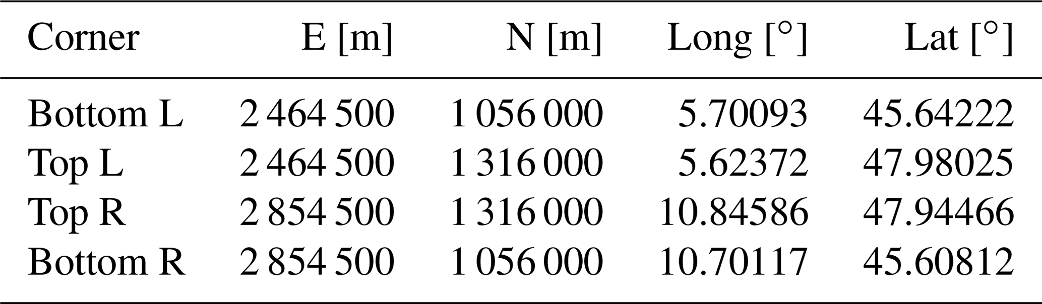
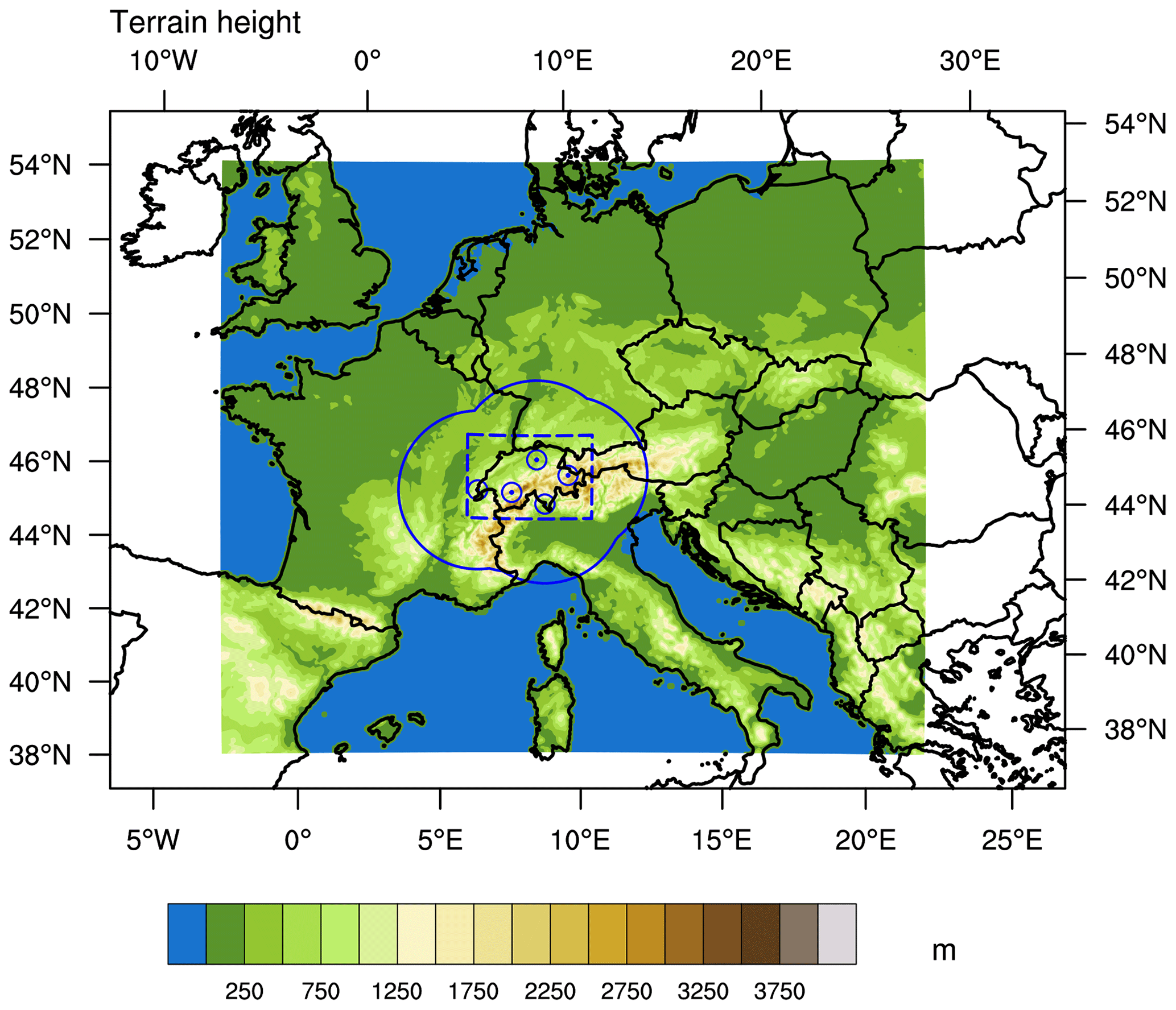
Figure 1Terrain heights (above sea level) for points covered by the WRF simulation outer domain. Black lines show national borders and coastlines. The locations of the five MeteoSwiss radars are indicated with blue circled points, and the solid blue line shows the approximate radar domain. The dashed blue line shows the study domain. Storms with centre points outside the study domain are not considered in this study. Elevations below 0.001 m are plotted in blue. Plot produced using the NCAR Command Language (NCL) version 6.6.2.
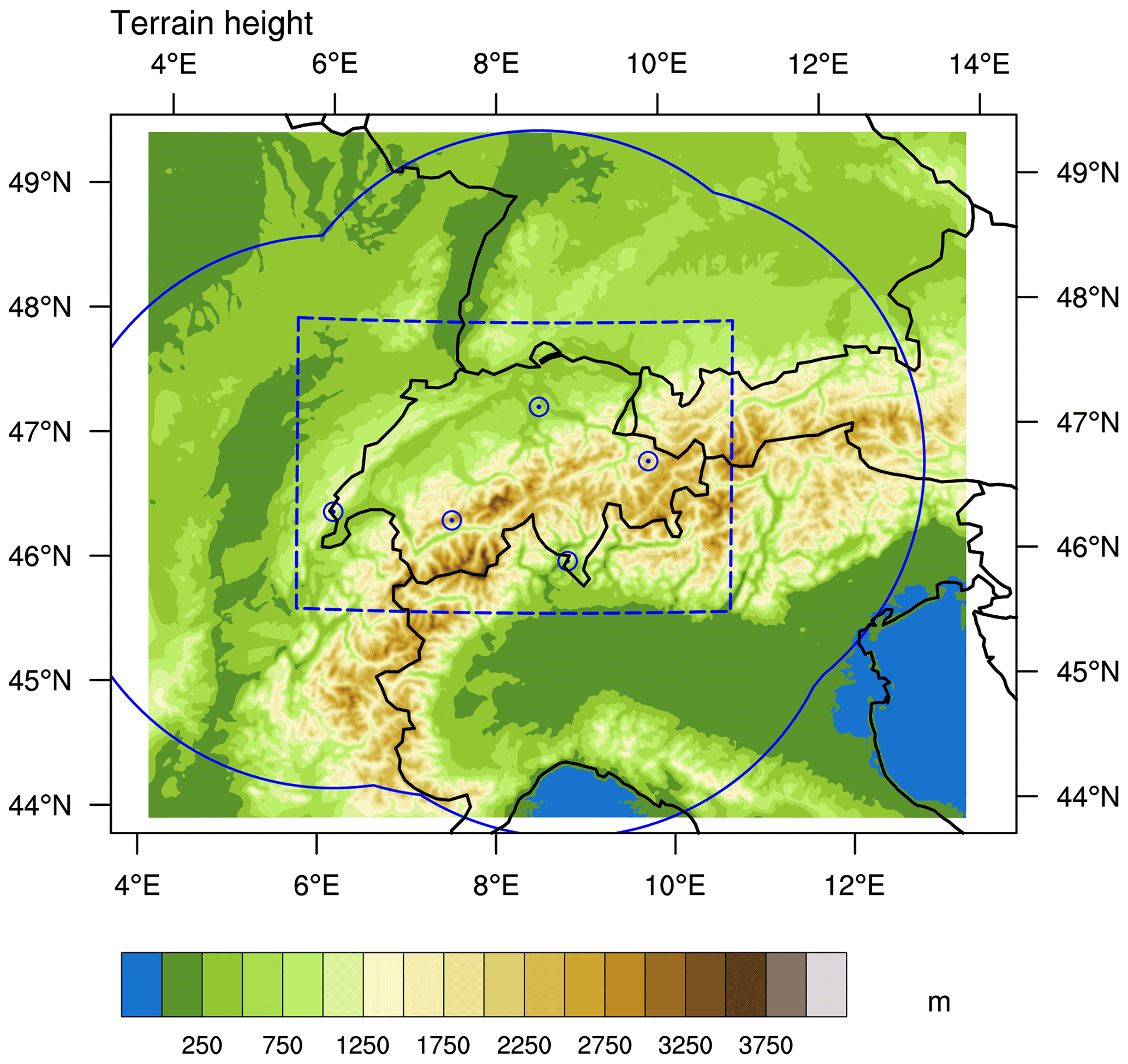
Figure 2As for Fig. 1, but for the inner (higher-resolution) nested WRF domain.
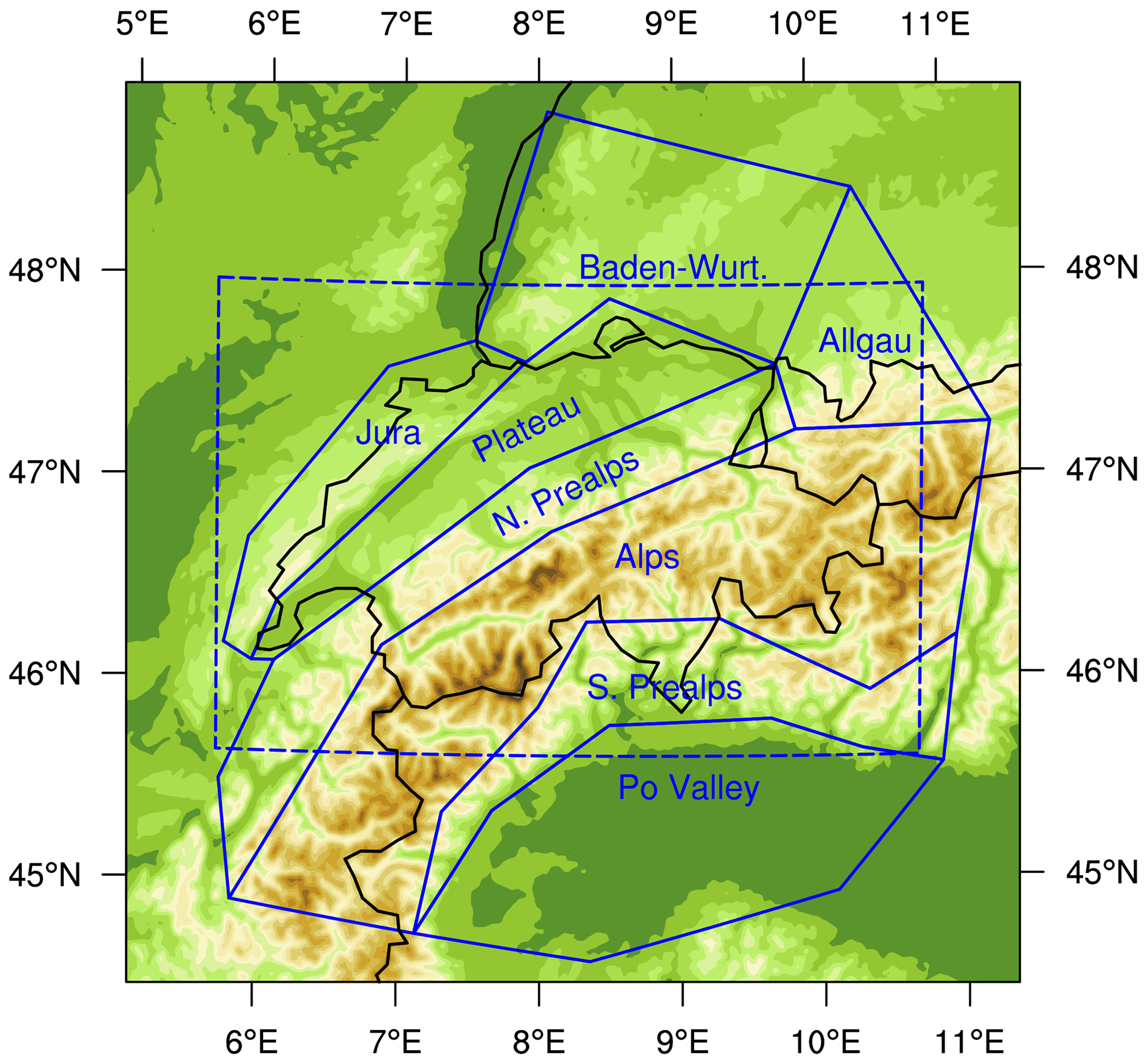
Figure 3Sub-domains used in this study (solid blue lines). Terrain elevation and national borders are shown as in Fig. 1. “N. Prealps” stands for northern Prealps, “S. Prealps” stands for southern Prealps, and “Baden-Wurt.” stands for Baden-Württemberg. The study domain is shown by the dashed blue line. Plot produced using NCL version 6.6.2.
2.2 Reference thunderstorm dataset
The reference data for thunderstorms in Switzerland are found in a database of thunderstorm tracking results compiled by MeteoSwiss. MeteoSwiss operates five C-band, dual-polarisation, Doppler weather radars in a network designed for high performance despite the challenges posed by the mountainous terrain of Switzerland (Germann et al., 2015). The resulting radar products are at high spatial and temporal resolution, with 20 elevation sweeps conducted every 5 min (Germann et al., 2015). The locations and approximate horizontal coverage area of the radar network are plotted in Figs. 1 and 2. The reference dataset we use in this study contains results from the TRT algorithm that were compiled into a database of storm cells and their associated properties (as in Nisi et al., 2018, but including data for 2018 and using all Swiss radars).
TRT was developed specifically to deal with the challenging topography of the Alpine region: it takes advantage of the high spatial and temporal resolution of the Swiss radar network (Nisi et al., 2016). TRT identifies thunderstorms in a two-dimensional Cartesian multiple-radar “max echo” composite product, which is composed of the maximum radar reflectivity recorded in each vertical column (Nisi et al., 2014). TRT uses an adaptive thresholding scheme proposed by Crane (1979) that requires a fixed minimum detection threshold Zmin [dBZ], a fixed minimum reflectivity “depth” Zdepth [dBZ], and an adaptive threshold Zthresh [dBZ]. On a two-dimensional map of max echo radar reflectivity, a cell is defined as a closed contour at Zthresh [dBZ] around a maximum reflectivity of Zpeak [dBZ]. Zthresh is adapted for each cell to be the minimum value for which Zthresh≥Zmin and for which the cell contains a single closed contour at Zpeak−Zdepth dBZ (Crane, 1979; Hering et al., 2004). In the case of TRT, Zmin is 36 dBZ and Zdepth is 6 dBZ, and a further constraint on cell area is applied: for a thunderstorm to be detected by TRT it must contain a connected area of sufficient size with radar reflectivity values at 36 dBZ or higher and at least one pixel with a reflectivity of at least 42 dBZ (Hering et al., 2004). The area threshold used in these observations was 13 km2 (Alessandro Hering, personal communication, 2020). TRT uses geographical overlapping of cells for matching between time steps (Hering et al., 2004, 2008). Several cell properties are then computed by TRT from the 3D radar data, as well as satellite and lightning data, inside the detected footprint of each cell. A cell severity ranking product is included.
TRT is well tested and established as a reference dataset. It has been in operational use at MeteoSwiss since 2003 (Hering et al., 2008) and formed part of a successful forecast demonstration project in the Alpine region (Rotach et al., 2009). TRT was used to produce a 15-year, Lagrangian-perspective hail climatology for Switzerland (Nisi et al., 2018), as well as to study hailstorm initiation with cold fronts (Schemm et al., 2016). In this study we use TRT results for the study period as the reference dataset. TRT code is not freely available, so in this study we use a generalised open-source storm tracker and compare its results to the state-of-the-art closed-source results of TRT.
2.3 The TITAN storm tracker
TITAN is a radar-based storm cell tracker that uses thresholds on 3D Cartesian fields of radar reflectivity to define contiguous storm areas, for which statistical properties are calculated (Dixon and Wiener, 1993). Matching of storms between time steps is performed using an optimisation algorithm that expects matched storms to have similar volumes and prioritises small separation distance (Dixon and Wiener, 1993). TITAN has been used operationally (e.g. Bally, 2004) and in an object-based study of hailstorm properties (Foris et al., 2006). We chose to use TITAN because of its free availability and long history of operational use; we note that other tracking methods are also available (e.g. Fridlind et al., 2019; Heikenfeld et al., 2019).

Figure 4The processing flowchart used in this study for WRF data. Shown are input data (blue)
processing steps (green) and analyses (yellow). Nc2Mdv is a modified version of the
TITAN tool NcGeneric2Mdv, and stormStats is a modified version of the TITAN tool
Storms2Xml2.
TITAN (Dixon and Wiener, 1993; TITAN system within LROSE, 2019) was downloaded and compiled
from the Lidar Radar Open Source Software Environment
(, ). TITAN uses specialised binary formats for both input
and output. As input, TITAN requires data in Meteorological Data Volume (MDV) format with radar
reflectivity fields in 3D Cartesian gridded coordinates
(Dixon and Wiener, 1993). We used an adapted version of the TITAN tool
NcGeneric2Mdv to convert input files to MDV format. The
outputs of the tracking process are “storm” files, in which the
tracking results are stored in binary format. To extract storm
properties from the storm files we used an adapted version of the
TITAN Storms2Xml2 tool. The TITAN processing flowchart for
simulation data is shown in Fig. 4.
For this study we ran TITAN in dual-thresholding mode with auto-restart disabled. In dual-thresholding mode, storms are identified in two steps. First, regions of reflectivity above a lower threshold are identified. Then, within these regions, areas with reflectivities greater than a sub-region reflectivity threshold are identified, tested for size, and “grown” out into the original lower-threshold region (Dixon and Seed, 2014). Threshold choice is discussed in Sect. 2.6.
2.4 WRF weather model
WRF is a weather model used for both research and operational numerical weather prediction (NWP) (Skamarock et al., 2019; Powers et al., 2017). When run at sufficiently high spatial resolution, it can explicitly resolve convection. What constitutes a sufficient resolution depends on the application: model grid spacings finer than 1 km are optimal for resolving all convective processes, while proper resolution of turbulent processes requires a grid spacing of the order of 100 m (e.g. Bryan et al., 2003; Bryan and Morrison, 2012). However, grid spacings up to 4 km provide enough detail to explicitly resolve basic cumulous cloud structures (e.g. Weisman et al., 1997; Done et al., 2004; Kain et al., 2006; Chevuturi et al., 2015). In this work we ran WRF with 50 vertical levels on a regional rotated grid with an average horizontal resolution of about 1.5×1.5 km2. A nested domain structure was used with a larger external domain at an average of about 4.6×4.6 km2 resolution. The two domains are shown in Figs. 1 and 2, respectively.
We used WRF version 4.0.1
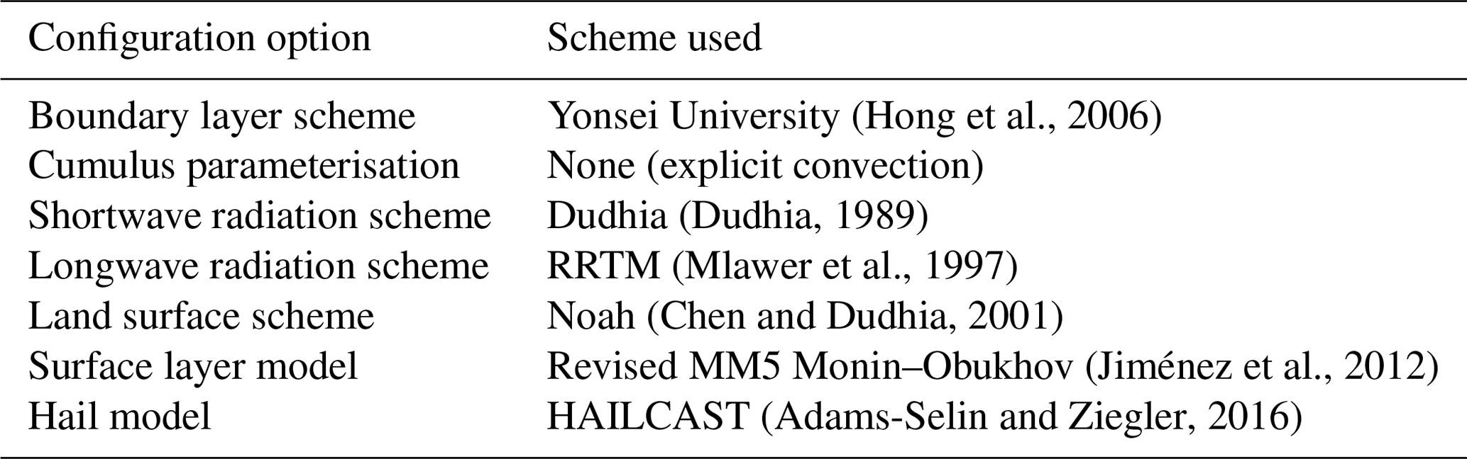
(Wang et al., 2018). HAILCAST (Brimelow et al., 2002; Adams-Selin and Ziegler, 2016) was used to calculate maximum hail sizes. We
tested three different WRF microphysics
schemes: the Predicted Particle Property (P3) scheme (Morrison and Milbrandt, 2015), the Morrison scheme (Morrison et al., 2009), and the Thompson scheme (Thompson et al., 2008). The other
schemes used in the model are shown in Table 2. The boundary data used were European Centre for
Medium-Range Weather Forecasts (ECMWF) operational analyses from the
Integrated Forecasting System (IFS) cycle 43r3 (ECMWF, 2017; Buizza et al., 2017). Radar reflectivity was calculated by WRF,
with the option do_radar_ref enabled to instruct WRF to
calculate reflectivity using microphysics-scheme-specific parameters
(Wang et al., 2018). The simulations covered May 2018 at
5 min
resolution.
Storm tracking was run on the WRF output variable REFL_10CM,
which contained estimated 10 cm wavelength (S-band) radar reflectivity
in decibels relative to reflectivity (dBZ) as produced by the WRF microphysics scheme. The WRF data were
treated using an NCAR command language (NCL, version 6.4.0, , ) script to regrid the data to a Cartesian grid stored
in NetCDF format. The files were first regridded horizontally by
dividing the WRF domain into a grid with the same number of points and
extents of latitude–longitude values as the input fields, but with the
points as evenly spaced as possible on each axis. The regridding was
performed using bilinear interpolation provided by the Earth System
Modeling Framework (ESMF, version 8.0.0; Valcke et al., 2012)
through NCL. The output grid had a resolution of approximately
0.0141∘ latitude by
0.0211∘ longitude. This grid was then
interpolated vertically using the NCL wrf_user_vert_interp
function to grid points from 1 to
15 km above sea level at 0.5 km
resolution. These heights were geopotential heights above sea level;
the small differences between geopotential and geometric heights are
ignored in this study. Interpolation of radar reflectivities was
performed using dBZ values. The regridded WRF files were converted to
MDV format for use with TITAN.
2.5 Comparing storm properties
Before comparisons of tracking results were made, TRT and TITAN cell detections with centre points outside the study domain (see Fig. 2) were discarded. Cells that were truncated by this operation had their durations shortened to the duration for which they stayed within the region of interest. Likewise, cells that were split into multiple parts by the spatial subsetting operation were updated so that their parts were counted as separate storm cells.
Thunderstorms often split into multiple parts or merge from multiple parts into single cells. TITAN and TRT handle the labelling of these storms differently. TITAN data contain a “storm ID” that is maintained through splits and merges and a “track ID”, which refers to a unique length of storm track with no splits or merges. TRT data contain flags indicating when splits and merges have occurred, and the most intense storm part keeps the same identifier afterwards. Due to these labelling differences, in this paper we take a simplified approach and refer to a “cell” as a region of high radar reflectivity that exists for at least 30 min with no splitting or merging events. When a split occurs, the parent cell ends and multiple new (child) cells are created, and when a merge occurs multiple cells end and a new (merged) cell is created. In this way we lose information on the overall length of one storm system, but we can compare cell properties easily and fairly. A “track” is the path over which a cell moves. A “cell detection” refers to a region of high reflectivity at one moment in time. Some storm properties (area, movement direction) are defined for each cell detection, while some (duration) are defined for each cell.
The TRT results are taken as the reference dataset, and TITAN results were compared to the TRT database to analyse the performance of the TITAN approach. The comparison measures used were defined as follows: for a given storm property P, let Pi,TITAN be the ith value of the property given by the TITAN approach and let Pi,TRT be the corresponding ith reference value of the property in the TRT database (i refers to an index shared by both datasets, such as simulation day). The difference between the two results is given by
The bias of the TITAN approach is 〈D〉, where the angular brackets signify the mean of all differences. The root mean squared error (RMSE) is . The relative error is given as a percentage by
The mean relative bias (RB, 〈R〉), the median relative bias (MRE, median of R), and the interquartile range of relative bias (RE IQR, 75th percentile minus 25th percentile of R) are used to measure relative differences. The squared Pearson correlation coefficient (r2) is used to show the co-fluctuation of PTITAN and PTRT. The relative error is only defined when Pi,TRT is non-zero; accordingly, RB, MRE, and RE IQR include only data points for which , whereas bias, RMSE, and r2 include such points. Days on which no technique identified cells are not counted in the statistics.
2.6 Optimisation of TITAN thresholds
Radar reflectivities simulated in WRF at S-band are not expected to match the measured radar reflectivities at C-band that were used by TRT, so we did not attempt to make TITAN use exactly the same thresholds as TRT. Furthermore, the TRT detection works on two-dimensional fields and thresholds on cell area, whereas TITAN uses three-dimensional fields and thresholds on cell volume. Our simulation setups differed only in the microphysics scheme used, but since the calculation of radar reflectivities can be affected by the microphysics scheme as well as the assumed radar frequency, optimum thresholds were expected to differ between simulation sets.
We chose to optimise three TITAN thresholds by finding the values that
provided the best match between TITAN+WRF (simulation) output and TRT
results (observations) for 29 and 30 May 2018, 2 d over which
thousands of storm detections were made across the domain. The
optimised thresholds were then used for validation of the technique with
the whole dataset for May 2018. The three thresholds tested were the following: (1) the reflectivity threshold for cell detection
(low_dbz_threshold in the TITAN parameter file), with
tested values from 34 to 42 dBZ in 1 dBZ increments; (2) the
reflectivity threshold for dual thresholding (dbz_threshold
under dual_threshold), with tested values from
low_dbz_threshold plus 4 dBZ to low_dbz_threshold
plus 12 dBZ in 1 dBZ increments; and (3) the volume threshold for cell
detection min_storm_size, with tested values of 25, 50, and
75 km3.
TITAN was run on WRF output for the test days with all 243 tested combinations of the three thresholds. The results for each run were compared to TRT results for those days. The “best” parameter set was non-trivial to select and depended on the performance metrics used. We chose an approach that emphasised low bias and co-fluctuation in the simulated and observed number of cells per hour and a good match for cell area. To choose the “winning” parameter set we used the absolute value of median relative bias as a score. This score was applied to comparisons of daily median cell area and per-time-step number of cells. We first subset based on the number of cells per hour by taking all test runs with scores less than the 10th percentile of all scores. We then subset based on daily median cell area by again taking scores less than the 10th percentile of all such scores. Of the few remaining tested combinations, we chose the configuration with the best squared correlation coefficient value for the simulated and observed per-time-step number of cells. The resulting thresholds used for TITAN tracking in this study are shown in Table 3. Reports showing details of the threshold testing are archived (Raupach et al., 2021d).
Other parameters in the dual-thresholding scheme were held fixed for
all model runs. These parameters were the minimum area required for
each sub-part in the dual-thresholding approach
(min_area_each_part), which was set to 16 km2, the
fraction of the lower-reflectivity storm region that must be covered
by the sum of all higher-reflectivity sub-regions
(min_fraction_all_parts), set to 0.10, and the minimum
proportion of the large area that each sub-area must exceed
(min_fraction_each_part), set to 0.005. These last two
area thresholds are those listed in the default TITAN parameters as
appropriate for strong convection and squall lines in South
Africa1.
In this section, storm properties found using TITAN with WRF simulation output are compared to those found using TRT with radar data to test whether TITAN applied to WRF simulations can produce representative statistics on thunderstorms in Switzerland. TITAN was run over the WRF simulation outputs, and TRT results were subset to the same period of time. Both sets of results were subset to the study domain shown by the dashed line in Figs. 1 and 2. During subsetting of the TITAN (TRT) results, including all tested microphysics scheme setups, subsetting caused splits in 0.78 % (0.64 %) of cells. After subsetting, 37.8 % (52.4 %) of the recorded cells were discarded because their track duration was less than 30 min. The resulting cell descriptions from TITAN sometimes contained spatial overlaps; 23 % of cells were affected by overlaps, but the areas affected were small, with only 3 % of all cell points overlapping. Of the TRT cells remaining after subsetting, 30 (0.06 %) were removed from this analysis because no cell velocity information was recorded.
Table 3The threshold values used in each application of TITAN. Other thresholds were left at default values. These thresholds are for the basic detection threshold (Z threshold, the low_dbz_threshold parameter), the dual-thresholding sub-region threshold (sub-region Z threshold, dual_threshold's dbz_threshold parameter), the minimum allowed storm volume (min. volume, the min_storm_size parameter), and the minimum area for sub-parts (min. sub-area, dual_threshold's min_area_each_part parameter).
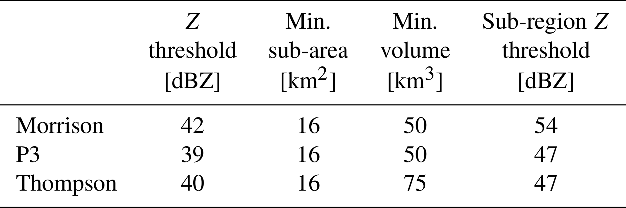
Table 4Summary information for each dataset, showing the number of cell detections (cell–time combinations), number of cells, and first and last cell detection times.

Table 4 shows a comparison of the number of detections (here defined as unique storm–time combinations) and storm cells captured by each technique. When each microphysics scheme was compared to the reference TRT dataset, TITAN produced 15 % more detections for the Morrison scheme, 9 % fewer detections for the P3 scheme, and 15 % fewer detections for the Thompson scheme. TITAN produced 4 % fewer cells for the Morrison scheme, 19 % fewer cells for the P3 scheme, and 19 % fewer cells for the Thompson scheme than were in the TRT dataset. In the rest of this section, we show detailed comparisons with sub-regions identified as shown in Fig. 3. The thunderstorm properties are divided into four categories: spatial and temporal cell occurrences (Sect. 3.1), cell movement properties (Sect. 3.2), hail properties (Sect. 3.3), and storm life cycle properties (Sect. 3.4).
3.1 Spatial and temporal cell occurrences
Figure 5 shows a comparison of the number of storm detections (cell–time combinations) per 10×10 km2 raster grid point to show the “hotspots” of storm activity during the month of May 2018 in both the simulations and observations. The figure shows broadly similar spatial layouts between observations and simulations. In particular, the observations and all simulations show regions of increased storm occurrence over the northern flanks of the Jura Mountains that run along the border of Switzerland and France, southwestern Germany, the southern Swiss Plateau and northern Prealps, and northern Italy to the east of Ticino (the part of Switzerland that extends into the southern Prealps region shown in Fig. 3). The simulated storm hotspots over the Jura are to the north of the observed Jura hotspot. Notably, the simulations all underestimate the concentration of storm detections in Ticino observed by radar. The simulations all reproduce the minima of storm activity that traces the main Alpine range; in this regard, the P3 and Thompson schemes produce more realistic maps than the Morrison scheme. Overall, the approach of using TITAN with WRF output is able to broadly reproduce the observed locations of cell detection maxima.
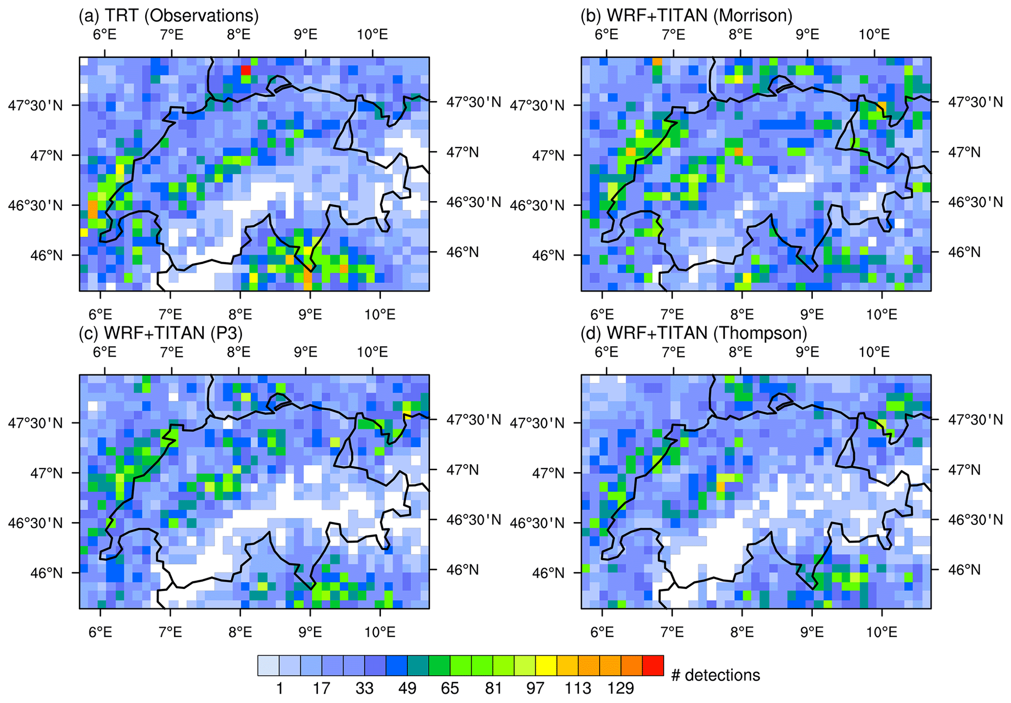
Figure 5The overall number of cell detections (cell–time combinations) in each 10×10 km2 grid point, for May 2018, for observations (a) and simulations with three different microphysics schemes (b–d). Plot produced using NCL version 6.6.2.
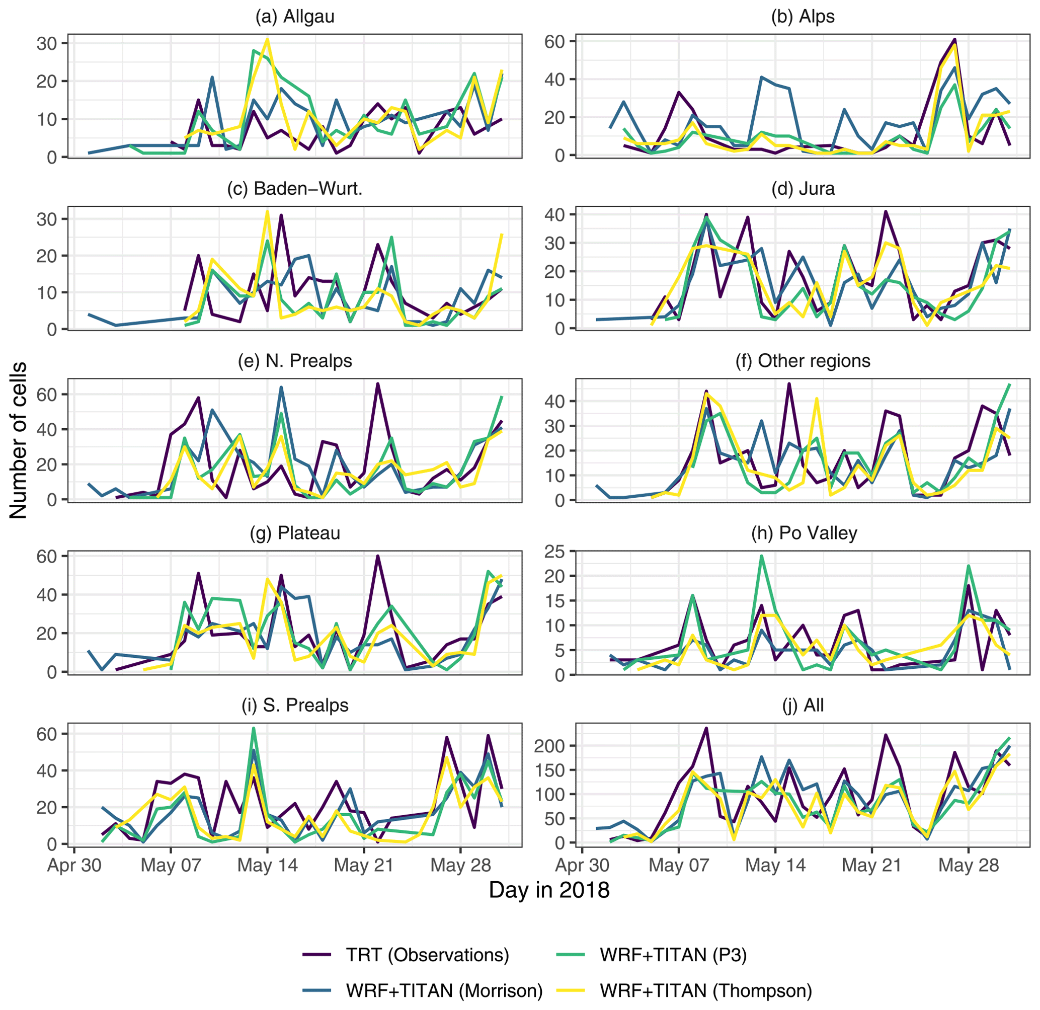
Figure 6The number of cells detected per day in May 2018 for observations and simulated outputs per region (regions shown in Fig. 3).
Table 5Performance statistics on cells detected per day per region, with TRT (observations) taken as the reference. Statistics shown are bias [d−1], root mean squared error (RMSE) [d−1], relative bias (RB) [%], median relative error (MRE) [%], interquartile range of relative error (RE IQR) [% points], and squared Pearson correlation (r2) [–].

Figure 6 shows the number of cells detected by each technique on each day of May 2018. Table 5 shows statistics to compare the number of cells per day between the simulations and observations. Because the simulations and observations are independent and the simulations are forced only by lower-resolution boundary conditions, we do not necessarily expect an exact match in cell occurrence time series. The simulated number of cells detected per day shows magnitudes similar to the observations, with exceptions in Allgäu, the Alps for the Morrison scheme, and the Po Valley for the P3 scheme, where more cells were detected in the simulations. In terms of median relative bias, the best per-region performance was with the Thompson scheme in the Alps region (−2 %), and the best performance for all regions combined was with the Morrison scheme (−13 %). The worst overall match was with the P3 scheme (−20 %). The worst per-region median relative bias was with the Morrison scheme in the Alps region (78 %). The greatest co-fluctuation (r2 value) in a single region was shown by the Thompson setup in the Alps region (0.74) and overall by the Thompson scheme (0.56). That positive correlations exist for cells per day shows that the WRF model is able to use these boundary conditions to produce thunderstorm cells on storm-prone days.
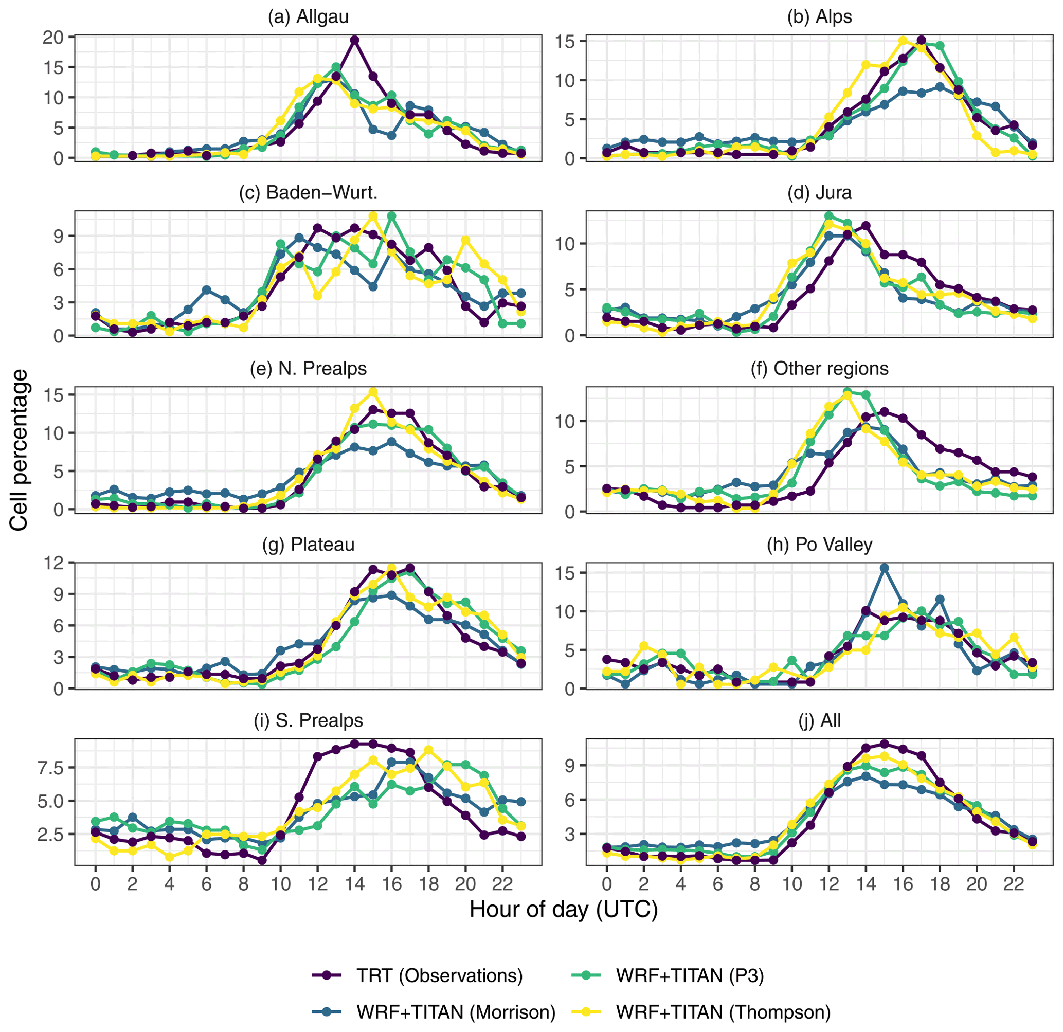
Figure 7Percentages of cells that were active in each hour of the day per region in May 2018, with observations compared to simulation outputs. Values are the percentage of all unique cell–hour combinations that occurred in each individual hour of the day so that values for each curve sum to 100.
To investigate any systematic timing differences and to look at the diurnal cycle of the thunderstorms, we calculated the percentage of cells that appeared in each hour of the day for each simulation and for the observations. These results are shown by region in Fig. 7. In all regions, the afternoon peak in thunderstorm activity is well reproduced by the simulations, although the exact timings differ from the observations in some regions. There is a tendency for the Morrison and P3 simulations to produce more cells during the night-time than are observed, and this continues into the morning for the Morrison scheme. For all data, the peak time for cell occurrence in the Thompson simulations matches the peak time in the observations, while the peak in the Morrison set is 1 h earlier, and there are peaks in the P3 scheme both 1 h earlier and 1 h later than the observed peak at 15:00 UTC. There is an interesting pattern in the results in which simulated storms tend to appear earlier than the observed storms in the north and northwest (Jura, Allgäu, other regions), at about the same time as the observations in central Switzerland (Alps, N. Prealps, plateau), and later than the observations in the southern Prealps. The results for the Po Valley match the observations well. Earlier storms in the north and later storms in the south have been shown in previous radar-based climatologies (Nisi et al., 2016), but here this effect is more extreme in the simulations than in the observations. The north-to-south differences are possibly due to different handling of convective initiation mechanisms in the weather model. There are known differences in storm initiation between northern regions of Switzerland and regions to the south of the main Alpine chain (Nisi et al., 2016, and references within).

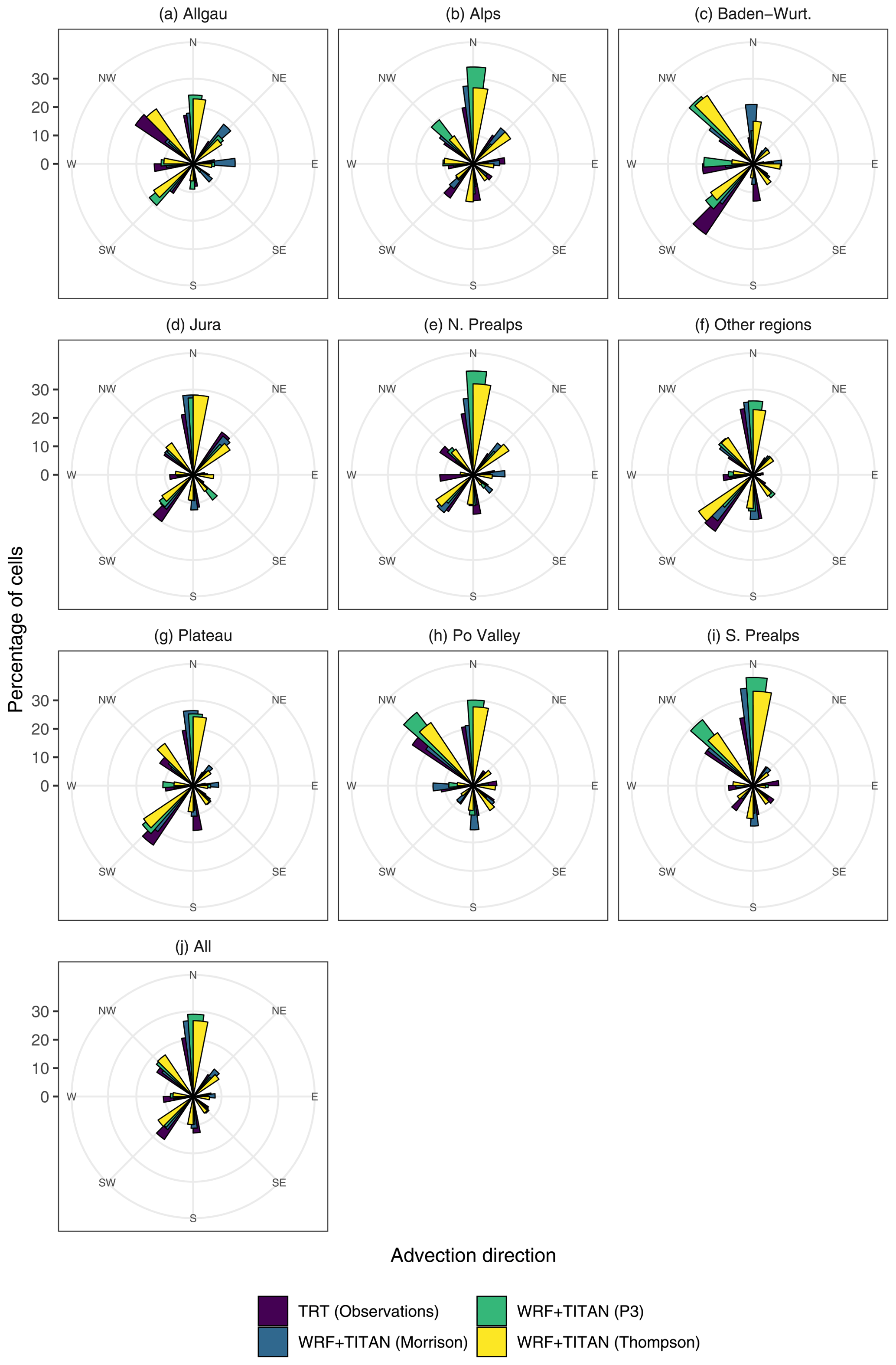
Figure 8Comparison of tracked cell directions by TITAN (on WRF data) and TRT (on radar observations). Shown are the percentages of times cells that were detected as moving in each of eight compass directions by dataset.
3.2 Cell movement properties
The use of object-based analysis means we can compare aggregate storm properties such as movement speed, direction, intensity, or cell lifetime. Figure 8 shows a comparison of the directions in which detected cells were moving at each observation point. Although there are some differences in the proportions between TRT and TITAN, it is notable that the simulations are able to reproduce the differences in advection direction observed between different regions. For example, the TRT observations show that storms moved mostly in a north and northwest direction in the Po Valley and in a southwest direction on the Swiss Plateau. The simulations reproduce these differences. Again, the region of Allgäu shows notable differences between observations and simulations. Table 6 shows the mean direction of all cells by region and dataset. The simulation set that produced the best match to observations differed by region, but the P3 scheme produced the best match in more regions than the other simulation sets.
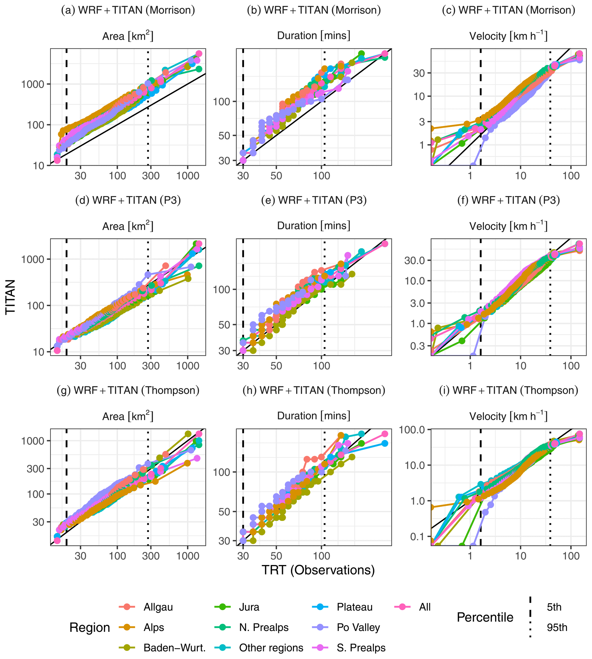
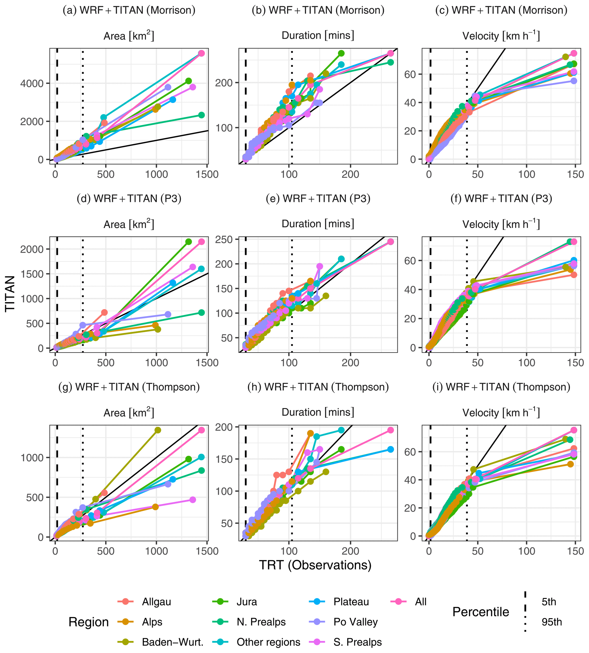
Figure 9Quantile-to-quantile (QQ) comparisons of cell detection areas, cell detection velocities, and cell durations by TITAN (in WRF simulations) and TRT (in radar observations). The black solid line is the 1:1 line. The vertical dashed lines show the 5th and 95th percentiles in the TRT distributions. Since the distributions are skewed, these plots are on logarithmic axes (zeros are plotted on the axis lines); the same plot with linear axes is shown for comparison in Fig. A1.
Figure 9 shows quantile-to-quantile (QQ) comparisons of three other properties: cell detection areas, cell detection velocities, and cell durations. We consider very high velocities (>80 km h−1) to be unrealistic artefacts of the tracking algorithms; for both TRT and TITAN + WRF results less than 0.5 % of cell detections had such velocities. We note again that these durations are the durations of cells as defined here, meaning that they are interrupted by storm splits and merges. The QQ plots map observed quantiles of these properties to simulated quantiles over all detected cells. If the simulated distributions match the observed distributions, the lines follow the diagonal (solid black) line on the QQ plot. The plot shows that the simulated distributions broadly agree with observed distributions for velocity in all simulations and for area and duration for the P3 and Thompson microphysics scheme setups. For the simulations run with Morrison microphysics, the plot shows that the detected cell areas were larger than the observed cells, and the simulated cells lasted for longer durations than the observed cells. Cell area and duration are most affected by the choice of thresholds used in the TITAN tracker, which means that these differences are unlikely to be caused by the microphysics scheme as such, but rather by the thresholds that result from the optimisation process described in Sect. 2.6.
3.3 Hail properties
In this section we compare radar-based observations of hail properties
to those estimated by the WRF model and HAILCAST. The object-based
technique we test here may be particularly useful for studying the
effects of climate change on hail, for which high
uncertainty remains (e.g. Raupach et al., 2021b). In each
dataset we compare the proportion of storm cell pixels that were
estimated to contain severe (greater than 2.5 cm) and very large
(greater than 4 cm) hail. In the observations from TRT, the maximum
hail size was estimated using the radar-based maximum expected severe
hail size (MESHS; implementation described
in Nisi et al., 2016). In the WRF output, we used the HAILCAST
variable HAILCAST_DIAM_MAX to calculate the proportions of
TITAN-identified cell pixels with hail over 2.5 and 4 cm,
respectively. We note that the two techniques used to estimate maximum
hail size are very different from each other and are therefore not
strictly directly comparable; they are used here as the available
approximations of observed and simulated hail size.
Table 7Proportions of total cell detections that contained hail with estimated diameter greater than 25 mm or 40 mm for observations and simulation outputs.
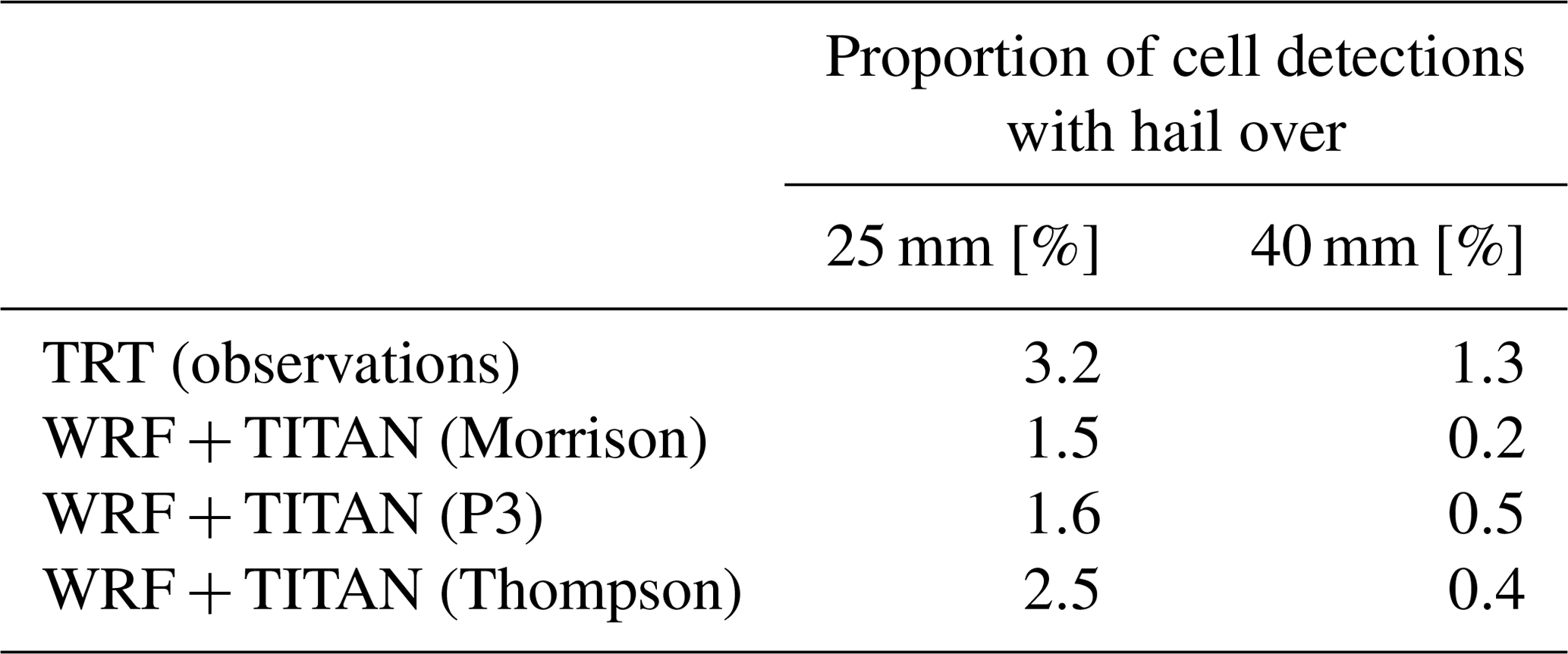
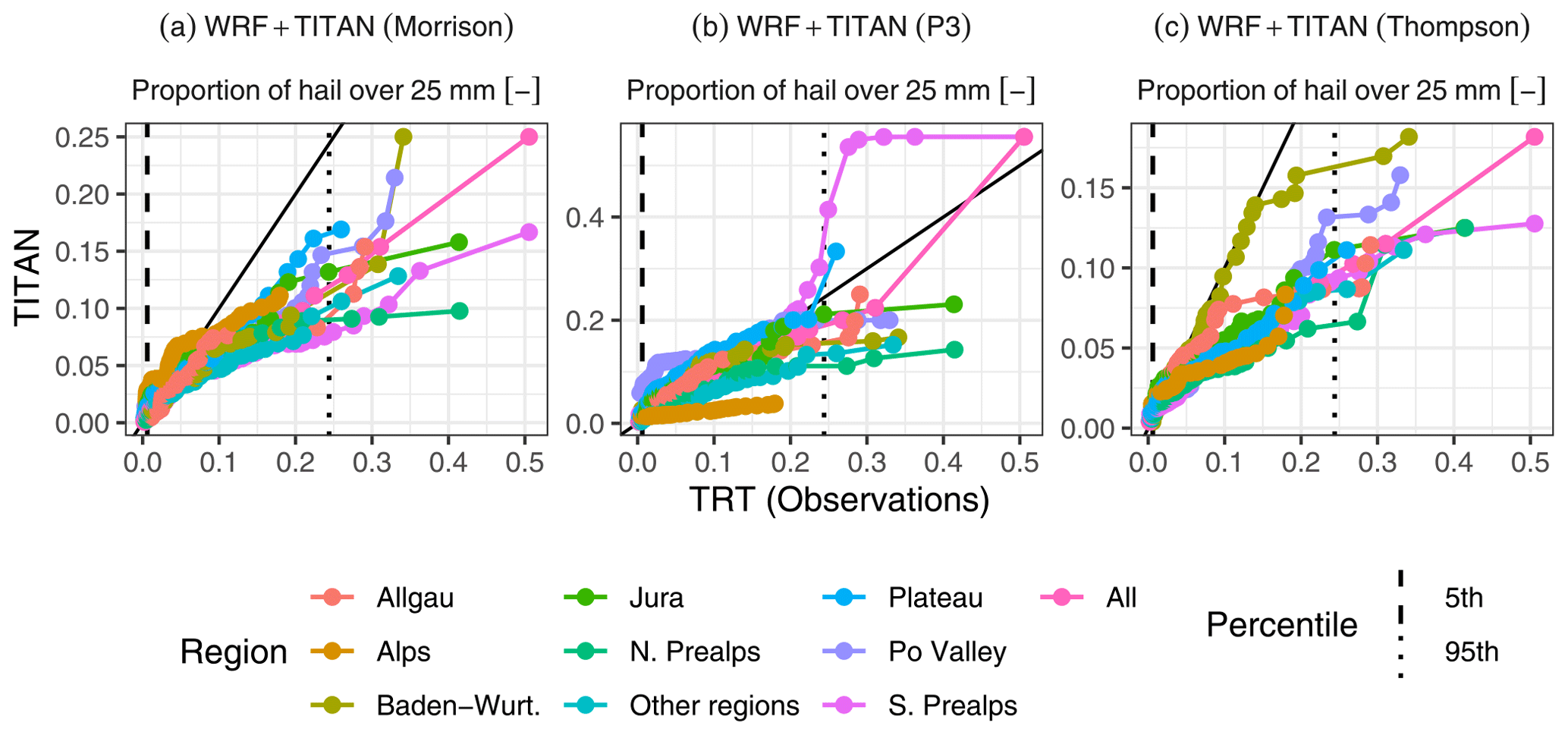
Figure 10Quantile-to-quantile (QQ) comparisons of the proportion of pixels with maximum hail size over 25 mm for cell detections for which this proportion was greater than zero. The black solid line is the 1:1 line. The vertical dashed lines show the 95th and 99th percentiles in the TRT distributions.
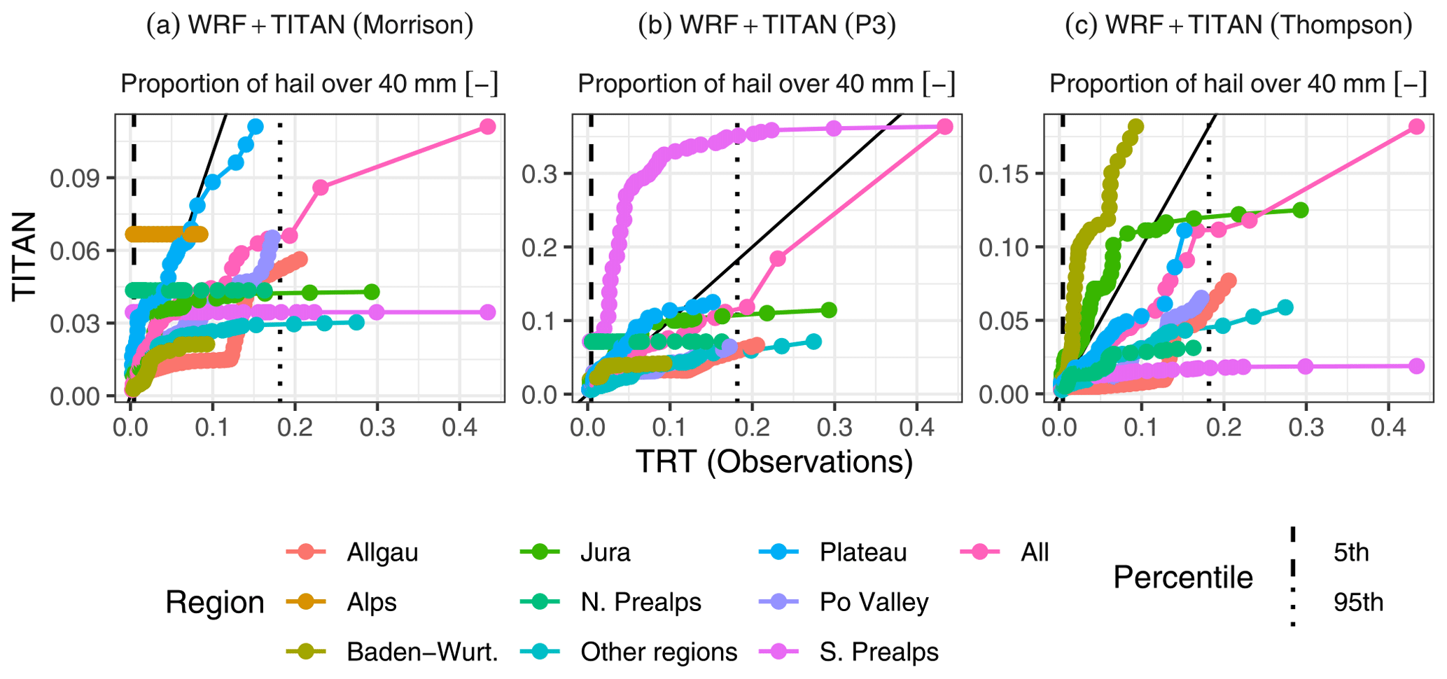

Figure 12The number of cells detected by cell duration for observations and simulation outputs.

Figure 13Area development over cell life cycles for observations and simulation outputs. For each time since the track start, the coloured band shows the interquartile range of area and the joined points show the median area.
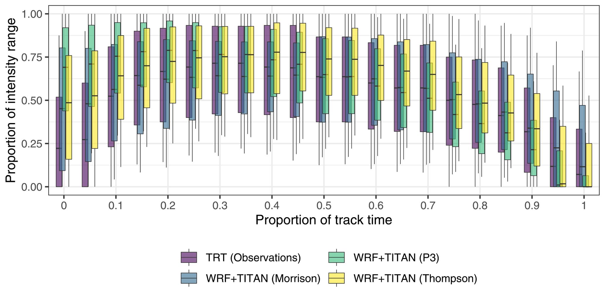
Figure 14Relative life cycle of storm cells. Vertical bars show distributions, with the middle marker showing the median, the coloured bar showing the IQR, and vertical lines showing the 10th to 90th percentile range.
Table 7 shows the proportions of all cell detections that contained severe hail. In general, the observations contained more severe hail than the simulations. All WRF setups underestimated the proportion of cell detections containing severe hail. The WRF setup using the Thompson microphysics scheme produced the closest match to the TRT proportion of cell detections with hail over 2.5 cm. The relative errors in these proportions were smaller for 2.5 cm hail than for 4 cm hail, implying that the WRF and HAILCAST simulations more severely underestimated the number of cells containing very large hail than severe hail. Figures 10 and 11 show quantile-to-quantile plots to compare the proportions of cell pixels, for cell detections for which the proportion was non-zero, that contained hail with maximum estimated size over 2.5 cm and over 4 cm, respectively. The WRF results show an underestimation of the cell area covered by severe and large hail compared to the TRT observations.
3.4 Cell life cycles
In this section we consider cell life cycles – the evolution of the strength of storm cells over their durations. Since in this work splits and merges of storms interrupt storm durations, in this section we consider only the 43 % of cells that contained no splits or merges so that their durations are well defined. Figure 12 shows the number of such cells by cell duration. There are very few cells with a duration over 100 min, meaning little emphasis should be placed on aggregate results for these long-duration cells. Figure 13 shows the development of cell area over time. The WRF simulations match the TRT observations well, with the exception of the Morrison scheme setup for which areas are overestimated at all points in the cell's life cycle. We emphasise, though, that since the area of cells at detection is defined by a threshold on storm size, the difference here has more to do with our optimised TITAN threshold values than with the microphysics scheme itself. The Thompson and P3 scheme setups provide a close match for cells up to about 100 min from their starting time. In Fig. 14, relative intensities of cells are compared to the relative positions in the cells' durations. Cells tracked in the simulations tend to reach their maximum intensities earlier than the observed cells but decay in a similar way. Differences between the different WRF setups are primarily in the first and last thirds of the storm life cycle, with the P3 scheme setup showing higher earlier intensities and earlier decay and the Morrison results showing the best match to observations from halfway through the track durations to about 85 % through the durations.
In this study we tested and verified an approach for the object-based analysis of simulated thunderstorms in the topographically complex Alpine region of Europe. Output from a high-resolution weather model (AR-WRF) was analysed using a radar storm tracking system (TITAN) to derive characteristics for each storm cell. The results were compared to a reliable and independently derived dataset of storm observations for Switzerland (TRT) for the month of May 2018. We tested WRF and TITAN using three different microphysics schemes.
The choice of radar reflectivity and cell volume thresholds to use in TITAN made a significant difference to the quality of the results. We optimised the thresholds to find the best settings to use for each microphysics scheme, but this search was location-dependent and not exhaustive; the resulting thresholds depended on which performance criteria were emphasised, and the search space over which thresholds are optimised could be further refined. The results of this study should thus not be seen as a comparison of the physical appropriateness of the microphysics schemes but a comparison of three possible setups (comprising both a scheme and chosen thresholds) for summarising thunderstorm properties in simulations over the Alpine region. TITAN thresholds, including those not optimised here such as the dual-thresholding scheme settings, should be carefully considered in any work that uses this technique. We used a simplified approach in which splits and merges in storm cells were ignored. Future work could take splits and merges into account in order to properly characterise full storm life cycles. Updates to TITAN have been suggested (e.g. Han et al., 2009; Muñoz et al., 2018) and could also be tested in future studies. We showed comparisons for simulated and radar-derived hail properties; in future, liquid precipitation could also be considered through the use of disaggregated precipitation fields (e.g. Barton et al., 2020). Further investigation would be required to analyse the sources of error where derived properties disagree. Possible error sources include the microphysics scheme and model resolution (e.g. as investigated in Australia by Caine et al., 2013), the model's ability to estimate the frequency of large-scale thunderstorm-prone environments (e.g. as investigated for the USA by Feng et al., 2021), and the radar frequency difference between observations and simulations. We also note that because we compared results from two different tracking algorithms (TITAN and TRT), tracking differences could not be separated from differences caused by model physics in this study. The many possible sources of difference between simulations and observations are one of the reasons that object-based analysis of thunderstorms is a useful approach in that it “abstracts away” the implementation details to attempt comparison of core storm properties instead.
The goal of this study was to determine whether TITAN plus WRF can provide a realistic representation of thunderstorm activity in Switzerland. The results show that a reasonable match between simulated and observed storm properties can be obtained if thresholds for TITAN cell detection are carefully chosen. The level of agreement between simulated and observed thunderstorm properties, for geographic distribution, diurnal cycle, number of cells per day, and cell area, duration, velocity, and movement direction, shows that WRF is able to explicitly resolve thunderstorm cell properties to an acceptable standard of accuracy at ∼1.5 km2 resolution over a topographically complex region. The simulations underestimated the occurrence of severe and very large hail. The approach of using TITAN to analyse storm properties produces results that are representative enough of the current climate to justify continuing use of the technique for comparisons between simulations of current and future scenarios. This technique therefore holds promise for investigation of how convective storms may be affected by climate change.
Code for this project is available under the MIT license at https://github.com/traupach/stormtrack (last access: 26 October 2021). Modified versions of LROSE utilities are available under the LROSE BSD license at https://github.com/traupach/modified_LROSE_utils (last access: 26 October 2021). Any code updates will be posted at these GitHub addresses. The exact versions of the code used to produce the results shown here are available as Zenodo archives for the original code (https://doi.org/10.5281/zenodo.4667884, Raupach et al., 2021d, MIT license), modified LROSE tools (https://doi.org/10.5281/zenodo.4667843, Raupach et al., 2021c, LROSE BSD license), and R Markdown for this paper (https://doi.org/10.5281/zenodo.5177686, Raupach et al., 2021e, CC-BY-4.0 license). TITAN tracking data and hail statistics extracted from WRF outputs are archived on Zenodo (https://doi.org/10.5281/zenodo.4638486, Raupach et al., 2021a, CC-BY-4.0 license). Fields of extracted WRF output (simulated radar reflectivity and maximum HAILCAST hail size) are archived on Zenodo for the Morrison (https://doi.org/10.5281/zenodo.4784820, Martinov et al., 2021a, CC-BY-4.0 license), P3 (https://doi.org/10.5281/zenodo.4808873, Martinov et al., 2021b, CC-BY-4.0 license), and Thompson (https://doi.org/10.5281/zenodo.4784811, Martinov et al., 2021c, CC-BY-4.0 license) microphysics schemes. Other WRF model output data are available from the authors by request. TRT data are proprietary to MeteoSwiss and are not publicly available; the contact details for MeteoSwiss are listed online (MeteoSwiss, 2021).
THR and OM designed the study. THR performed the analyses and wrote the paper. AM configured and ran WRF to produce model output. LN and AH provided expert advice on TRT. YB compiled TRT data. All authors provided feedback on the paper.
Timothy H. Raupach (until 31 December 2019), Olivia Martius (ongoing), Andrey Martynov (until 31 May 2021), and Yannick Barton (ongoing) were in positions funded by the Mobiliar Insurance Group. This funding source played no role in any part of the study.
Publisher's note: Copernicus Publications remains neutral with regard to jurisdictional claims in published maps and institutional affiliations.
The authors thank MeteoSwiss and Urs Germann for providing the TRT storm database. Simulations were calculated on UBELIX (http://www.id.unibe.ch/hpc, last access: 18 October 2021), the HPC cluster at the University of Bern.
This paper was edited by Paul Ullrich and reviewed by Scott Collis and one anonymous referee.
Adams-Selin, R. D. and Ziegler, C. L.: Forecasting Hail Using a One-Dimensional Hail Growth Model within WRF, Mon. Weather Rev., 144, 4919–4939, https://doi.org/10.1175/MWR-D-16-0027.1, 2016. a, b
Allen, J. T.: Climate change and severe thunderstorms, in: Oxford Research Encyclopedia of Climate Science, Oxford University Press, https://doi.org/10.1093/acrefore/9780190228620.013.62, 2018. a, b
Bally, J.: The Thunderstorm Interactive Forecast System: Turning Automated Thunderstorm Tracks into Severe Weather Warnings, Weather Forecast., 19, 64–72, https://doi.org/10.1175/1520-0434(2004)019<0064:TTIFST>2.0.CO;2, 2004. a
Barton, Y., Sideris, I. V., Raupach, T. H., Gabella, M., Germann, U., and Martius, O.: A multi-year assessment of sub-hourly gridded precipitation for Switzerland based on a blended radar – Rain-gauge dataset, Int. J. Climatol., 40, 5208–5222, https://doi.org/10.1002/joc.6514, 2020. a
Brimelow, J. C., Reuter, G. W., and Poolman, E. R.: Modeling Maximum Hail Size in Alberta Thunderstorms, Weather Forecast., 17, 1048–1062, https://doi.org/10.1175/1520-0434(2002)017<1048:MMHSIA>2.0.CO;2, 2002. a
Bryan, G. H. and Morrison, H.: Sensitivity of a Simulated Squall Line to Horizontal Resolution and Parameterization of Microphysics, Mon. Weather Rev., 140, 202–225, https://doi.org/10.1175/MWR-D-11-00046.1, 2012. a
Bryan, G. H., Wyngaard, J. C., and Fritsch, J. M.: Resolution Requirements for the Simulation of Deep Moist Convection, Mon. Weather Rev., 131, 2394–2416, https://doi.org/10.1175/1520-0493(2003)131<2394:RRFTSO>2.0.CO;2, 2003. a, b
Buizza, R., Bechtold, P., Bonavita, M., Bormann, N., Bozzo, A., Haiden, T., Hogan, R., Hólm, E., Radnoti, G., Richardson, D., and Sleigh, M.: IFS Cycle 43r3 brings model and assimilation updates, European Centre for Medium-Range Weather Forecasts, Reading, UK, 18–22, https://doi.org/10.21957/76t4e1, 2017. a
Caine, S., Lane, T. P., May, P. T., Jakob, C., Siems, S. T., Manton, M. J., and Pinto, J.: Statistical Assessment of Tropical Convection-Permitting Model Simulations Using a Cell-Tracking Algorithm, Mon. Weather Rev., 141, 557–581, https://doi.org/10.1175/MWR-D-11-00274.1, 2013. a, b, c, d
CH2018: CH2018 – Climate Scenarios for Switzerland, Technical Report, National Centre for Climate Services, Zurich, Switzerland, 271 pp., 2018. a, b
Chen, F. and Dudhia, J.: Coupling an Advanced Land Surface–Hydrology Model with the Penn State–NCAR MM5 Modeling System. Part I: Model Implementation and Sensitivity, Mon. Weather Rev., 129, 569–585, https://doi.org/10.1175/1520-0493(2001)129<0569:CAALSH>2.0.CO;2, 2001. a
Chevuturi, A., Dimri, A. P., Das, S., Kumar, A., and Niyogi, D.: Numerical simulation of an intense precipitation event over Rudraprayag in the central Himalayas during 13–14 September 2012, J. Earth. Syst. Sci., 124, 1545–1561, https://doi.org/10.1007/s12040-015-0622-5, 2015. a
Collins, M., Knutti, R., Arblaster, J., Dufresne, J.-L., Fichefet, T., Friedlingstein, P., Gao, X., Gutowski, W., Johns, T., Krinner, G., Shongwe, M., Tebaldi, C., Weaver, A., and Wehner, M.: Long-term Climate Change: Projections, Commitments and Irreversibility, in: Climate Change 2013: The Physical Science Basis. Contribution of Working Group I to the Fifth Assessment Report of the Intergovernmental Panel on Climate Change, edited by Stocker, T., Qin, D., Plattner, G.-K., Tignor, M., Allen, S., Boschung, J., Nauels, A., Xia, Y., Bex, V., and Midgley, P., Cambridge University Press, Cambridge, United Kingdom and New York, NY, USA, 2013. a
Crane, R. K.: Automatic Cell Detection and Tracking, IEEE T. Geosci. Elect., 17, 250–262, https://doi.org/10.1109/TGE.1979.294654, 1979. a, b
Davis, C., Brown, B., and Bullock, R.: Object-Based Verification of Precipitation Forecasts. Part I: Methodology and Application to Mesoscale Rain Areas, Mon. Weather Rev., 134, 1772–1784, https://doi.org/10.1175/MWR3145.1, 2006a. a
Davis, C., Brown, B., and Bullock, R.: Object-Based Verification of Precipitation Forecasts. Part II: Application to Convective Rain Systems, Mon. Weather Rev., 134, 1785–1795, https://doi.org/10.1175/MWR3146.1, 2006b. a
Diffenbaugh, N. S., Scherer, M., and Trapp, R. J.: Robust increases in severe thunderstorm environments in response to greenhouse forcing, P. Natl. Acad. Sci. USA, 110, 16361–16366, https://doi.org/10.1073/pnas.1307758110, 2013. a
Dixon, M. and Seed, A.: Developments in echo tracking-enhancing TITAN, in: Proceedings of the ERAD2014 – The Eighth European Conference on Radar in Meteorology and Hydrology, Garmisch-Partenkirchen, Germany, vol. 15, 2014. a
Dixon, M. and Wiener, G.: TITAN: Thunderstorm Identification, Tracking, Analysis, and Nowcasting – A Radar-based Methodology, J. Atmos. Ocean Tech., 10, 785–797, https://doi.org/10.1175/1520-0426(1993)010<0785:TTITAA>2.0.CO;2, 1993. a, b, c, d, e, f
Done, J., Davis, C. A., and Weisman, M.: The next generation of NWP: explicit forecasts of convection using the weather research and forecasting (WRF) model, Atmos. Sci. Lett., 5, 110–117, https://doi.org/10.1002/asl.72, 2004. a, b
Dudhia, J.: Numerical Study of Convection Observed during the Winter Monsoon Experiment Using a Mesoscale Two-Dimensional Model, J. Atmos. Sci., 46, 3077–3107, https://doi.org/10.1175/1520-0469(1989)046<3077:NSOCOD>2.0.CO;2, 1989. a
Ebert, E. E.: Neighborhood Verification: A Strategy for Rewarding Close Forecasts, Weather Forecast., 24, 1498–1510, https://doi.org/10.1175/2009WAF2222251.1, 2009. a, b
ECMWF: European Centre for Medium-Range Weather Forecasts (ECMWF)’s Integrated Forecasting System (IFS), cycle 43r3, available at: https://www.ecmwf.int/en/forecasts/documentation/evolution-ifs/cycles/cycle-43r3 (last access: 18 October 2021), 2017. a
Feng, Z., Leung, L. R., Houze Jr., R. A., Hagos, S., Hardin, J., Yang, Q., Han, B., and Fan, J.: Structure and Evolution of Mesoscale Convective Systems: Sensitivity to Cloud Microphysics in Convection-Permitting Simulations Over the United States, J. Adv. Model. Earth Sy., 10, 1470–1494, https://doi.org/10.1029/2018MS001305, 2018. a, b
Feng, Z., Houze, R. A., Leung, L. R., Song, F., Hardin, J. C., Wang, J., Gustafson, W. I., and Homeyer, C. R.: Spatiotemporal characteristics and large-scale environments of mesoscale convective systems east of the Rocky Mountains, J. Climate, 32, 7303–7328, https://doi.org/10.1175/JCLI-D-19-0137.1, 2019. a
Feng, Z., Song, F., Sakaguchi, K., and Leung, L. R.: Evaluation of Mesoscale Convective Systems in Climate Simulations: Methodological Development and Results from MPAS-CAM over the United States, J. Climate, 34, 2611–2633, https://doi.org/10.1175/JCLI-D-20-0136.1, 2021. a, b
Foris, D. V., Karacostas, T. S., Flocas, A. A., and Makrogiannis, T. I.: Hailstorm in the region of Central Macedonia, Greece: a kinematic study, Meteorol. Z., 15, 317–326, https://doi.org/10.1127/0941-2948/2006/0134, 2006. a
Fridlind, A. M., van Lier-Walqui, M., Collis, S., Giangrande, S. E., Jackson, R. C., Li, X., Matsui, T., Orville, R., Picel, M. H., Rosenfeld, D., Ryzhkov, A., Weitz, R., and Zhang, P.: Use of polarimetric radar measurements to constrain simulated convective cell evolution: a pilot study with Lagrangian tracking, Atmos. Meas. Tech., 12, 2979–3000, https://doi.org/10.5194/amt-12-2979-2019, 2019. a, b
Germann, U., Boscacci, M., Gabella, M., and Sartori, M.: Peak performance: Radar design for prediction in the Swiss Alps, Meteorol. Technol. Int, 4, 42–45, 2015. a, b, c, d
Gilleland, E., Ahijevych, D. A., Brown, B. G., and Ebert, E. E.: Verifying Forecasts Spatially, B. Am. Meteorol. Soc., 91, 1365–1376, https://doi.org/10.1175/2010BAMS2819.1, 2010. a, b, c
Han, L., Fu, S., Zhao, L., Zheng, Y., Wang, H., and Lin, Y.: 3D Convective Storm Identification, Tracking, and Forecasting–An Enhanced TITAN Algorithm, J. Atmos. Ocean Tech., 26, 719–732, https://doi.org/10.1175/2008JTECHA1084.1, 2009. a
Hartmann, D., Tank, A. K., Rusticucci, M., Alexander, L., Brönnimann, S., Charabi, Y., Dentener, F., Dlugokencky, E., Easterling, D., Kaplan, A., Soden, B., Thorne, P., Wild, M., and Zhai, P.: Observations: Atmosphere and Surface, in: Climate Change 2013: The Physical Science Basis. Contribution of Working Group I to the Fifth Assessment Report of the Intergovernmental Panel on Climate Change, edited by: Stocker, T., Qin, D., Plattner, G.-K., Tignor, M., Allen, S., Boschung, J., Nauels, A., Xia, Y., Bex, V., and Midgley, P., Cambridge University Press, Cambridge, United Kingdom and New York, NY, USA, 2013. a
Heikenfeld, M., Marinescu, P. J., Christensen, M., Watson-Parris, D., Senf, F., van den Heever, S. C., and Stier, P.: tobac 1.2: towards a flexible framework for tracking and analysis of clouds in diverse datasets, Geosci. Model Dev., 12, 4551–4570, https://doi.org/10.5194/gmd-12-4551-2019, 2019. a, b
Hering, A. M., Morel, C., Galli, G., Sénési, S., Ambrosetti, P., and Boscacci, M.: Nowcasting thunderstorms in the Alpine region using a radar based adaptive thresholding scheme, in: Proceedings of the 3rd European Conference on Radar in Meteorology and Hydrology, 206–211, Copernicus, available at: http://www.copernicus.org/erad/2004/online/ERAD04_P_206.pdf (last access: 18 August 2018), 2004. a, b, c, d, e
Hering, A. M., Germann, U., Boscacci, M., and Sénési, S.: Operational nowcasting of thunderstorms in the Alps during MAP D-PHASE, in: Proceedings of the 5th European Conference on Radar in Meteorology and Hydrology, 30 June–4 July 2008, Helsinki, Finland, 2008. a, b, c
Hong, S.-Y., Noh, Y., and Dudhia, J.: A New Vertical Diffusion Package with an Explicit Treatment of Entrainment Processes, Mon. Weather Rev., 134, 2318–2341, https://doi.org/10.1175/MWR3199.1, 2006. a
Houze Jr., R. A.: Orographic effects on precipitating clouds, Rev. Geophys., 50, RG1001, https://doi.org/10.1029/2011RG000365, 2012. a
Houze, R. A., Schmid, W., Fovell, R. G., and Schiesser, H.-H.: Hailstorms in Switzerland: Left Movers, Right Movers, and False Hooks, Mon. Weather Rev., 121, 3345–3370, https://doi.org/10.1175/1520-0493(1993)121<3345:HISLMR>2.0.CO;2, 1993. a, b
Jiménez, P. A., Dudhia, J., González-Rouco, J. F., Navarro, J., Montávez, J. P., and García-Bustamante, E.: A Revised Scheme for the WRF Surface Layer Formulation, Mon. Weather Rev., 140, 898–918, https://doi.org/10.1175/MWR-D-11-00056.1, 2012. a
Kain, J. S., Weiss, S. J., Levit, J. J., Baldwin, M. E., and Bright, D. R.: Examination of Convection-Allowing Configurations of the WRF Model for the Prediction of Severe Convective Weather: The SPC/NSSL Spring Program 2004, Weather Forecast., 21, 167–181, https://doi.org/10.1175/WAF906.1, 2006. a
LROSE: LROSE – The Lidar Radar Open Software Environment, available at: https://github.com/NCAR/lrose-core, git version lrose-cyclone-20190801-167-g85b01e9a3, last access: 12 November 2019. a
Madonna, E., Ginsbourger, D., and Martius, O.: A Poisson regression approach to model monthly hail occurrence in Northern Switzerland using large-scale environmental variables, Atmos. Res., 203, 261–274, https://doi.org/10.1016/j.atmosres.2017.11.024, 2018. a
Martinov, A., Raupach, T. H., and Martius, O.: WRF model fields for TITAN tracking of simulated storms, Morrison microphysics scheme, Zenodo [data set], https://doi.org/10.5281/zenodo.4784820, 2021a. a
Martinov, A., Raupach, T. H., and Martius, O.: WRF model fields for TITAN tracking of simulated storms, P3 microphysics scheme, Zenodo [data set], https://doi.org/10.5281/zenodo.4808873, 2021b. a
Martinov, A., Raupach, T. H., and Martius, O.: WRF model fields for TITAN tracking of simulated storms, Thompson microphysics scheme, Zenodo [data set], https://doi.org/10.5281/zenodo.4784811, 2021c. a
Martius, O., Hering, A., Kunz, M., Manzato, A., Mohr, S., Nisi, L., and Trefalt, S.: Challenges and Recent Advances in Hail Research, B. Am. Meteorol. Soc., 99, ES51–ES54, https://doi.org/10.1175/BAMS-D-17-0207.1, 2018. a
MétéoSuisse: Bulletin climatologique juin 2018, Tech. rep., MétéoSuisse, Genève, available at: https://www.meteosuisse.admin.ch/content/dam/meteoswiss/fr/service-und-publikationen/publikationen/doc/201806_f.pdf, last access: 26 November 2018a. a
MétéoSuisse: Bulletin climatologique mai 2018, Tech. rep., MétéoSuisse, Genève, available at: https://www.meteosuisse.admin.ch/content/dam/meteoswiss/fr/service-und-publikationen/publikationen/doc/201805_f.pdf, last access: 26 November 2018b. a, b, c
MétéoSuisse: Bulletin climatologique été 2018, Tech. rep., MétéoSuisse, Genève, available at: https://www.meteosuisse.admin.ch/content/dam/meteoswiss/fr/service-und-publikationen/publikationen/doc/2018_JJA_f.pdf, last access: 20 December 2018c. a
MeteoSwiss: Contact – MeteoSwiss, available at: https://www.meteoswiss.admin.ch/home/about-us/contact.html, last access: 27 May 2021. a
Mlawer, E. J., Taubman, S. J., Brown, P. D., Iacono, M. J., and Clough, S. A.: Radiative transfer for inhomogeneous atmospheres: RRTM, a validated correlated-k model for the longwave, J. Geophys. Res.-Atmos., 102, 16663–16682, https://doi.org/10.1029/97JD00237, 1997. a
Morrison, H. and Milbrandt, J. A.: Parameterization of Cloud Microphysics Based on the Prediction of Bulk Ice Particle Properties. Part I: Scheme Description and Idealized Tests, J. Atmos. Sci., 72, 287–311, https://doi.org/10.1175/JAS-D-14-0065.1, 2015. a
Morrison, H., Thompson, G., and Tatarskii, V.: Impact of Cloud Microphysics on the Development of Trailing Stratiform Precipitation in a Simulated Squall Line: Comparison of One- and Two-Moment Schemes, Mon. Weather Rev., 137, 991–1007, https://doi.org/10.1175/2008MWR2556.1, 2009. a
Muñoz, C., Wang, L.-P., and Willems, P.: Enhanced object-based tracking algorithm for convective rain storms and cells, Atmos. Res., 201, 144–158, https://doi.org/10.1016/j.atmosres.2017.10.027, 2018. a
NCL6.4: The NCAR Command Language, version 6.4.0, UCAR/NCAR/CISL/TDD [code], Boulder, Colorado, https://doi.org/10.5065/D6WD3XH5, 2017. a
Nisi, L., Ambrosetti, P., and Clementi, L.: Nowcasting severe convection in the Alpine region: the COALITION approach, Q. J. Roy. Meteor. Soc., 140, 1684–1699, https://doi.org/10.1002/qj.2249, 2014. a
Nisi, L., Martius, O., Hering, A., Kunz, M., and Germann, U.: Spatial and temporal distribution of hailstorms in the Alpine region: a long-term, high resolution, radar-based analysis, Q. J. Roy. Meteor. Soc., 142, 1590–1604, https://doi.org/10.1002/qj.2771, 2016. a, b, c, d, e, f, g
Nisi, L., Hering, A., Germann, U., and Martius, O.: A 15-year hail streak climatology for the Alpine region, Q. J. Roy. Meteor. Soc., 144, 1429–1449, https://doi.org/10.1002/qj.3286, 2018. a, b, c, d, e
Peyraud, L.: Analysis of the 18 July 2005 Tornadic Supercell over the Lake Geneva Region, Weather Forecast., 28, 1524–1551, https://doi.org/10.1175/WAF-D-13-00022.1, 2013. a
Pinto, J., Phillips, C., Steiner, M., Rasmussen, R., Oien, N., Dixon, M., Wang, W., and Weisman, M.: Assessment of the statistical characteristics of thunderstorms simulated with the WRF model using convection-permitting resolution, in: Proceedings of the 33rd Conf. on Radar Meteorology, Cairns, Australia, Amer. Meteorol. Soc., available at: https://ams.confex.com/ams/pdfpapers/123712.pdf (last access: 14 August 2018), 2007. a, b
Powers, J. G., Klemp, J. B., Skamarock, W. C., Davis, C. A., Dudhia, J., Gill, D. O., Coen, J. L., Gochis, D. J., Ahmadov, R., Peckham, S. E., Grell, G. A., Michalakes, J., Trahan, S., Benjamin, S. G., Alexander, C. R., Dimego, G. J., Wang, W., Schwartz, C. S., Romine, G. S., Liu, Z., Snyder, C., Chen, F., Barlage, M. J., Yu, W., and Duda, M. G.: The Weather Research and Forecasting Model: Overview, System Efforts, and Future Directions, B. Am. Meteorol. Soc., 98, 1717–1737, https://doi.org/10.1175/BAMS-D-15-00308.1, 2017. a
Punge, H. and Kunz, M.: Hail observations and hailstorm characteristics in Europe: A review, Atmos. Res., 176–177, 159–184, https://doi.org/10.1016/j.atmosres.2016.02.012, 2016. a
Punge, H., Bedka, K., Kunz, M., and Reinbold, A.: Hail frequency estimation across Europe based on a combination of overshooting top detections and the ERA-INTERIM reanalysis, Atmos. Res., 198, 34–43, https://doi.org/10.1016/j.atmosres.2017.07.025, 2017. a
Raupach, T. H., Martinov, A., and Martius, O.: Thunderstorm tracks and hail properties derived from WRF simulation data for May 2018 over Switzerland, Zenodo [data set], https://doi.org/10.5281/zenodo.4638486, 2021a. a
Raupach, T. H., Martius, O., Allen, J. T., Kunz, M., Lasher-Trapp, S., Mohr, S., Rasmussen, K. L., Trapp, R. J., and Zhang, Q.: The effects of climate change on hailstorms, Nat. Rev. Earth Environ., 2, 213–226, https://doi.org/10.1038/s43017-020-00133-9, 2021b. a, b
Raupach, T. H., Martynov, A., and Martius, O.: traupach/modified_LROSE_utils: Initial release, Zenodo [code], https://doi.org/10.5281/zenodo.4667843, 2021c. a
Raupach, T. H., Martynov, A., and Martius, O.: traupach/stormtrack: Initial release, Zenodo [code], https://doi.org/10.5281/zenodo.4667884, 2021d. a, b
Raupach, T. H., Martynov, A., Nisi, L., Hering, A., Barton, Y., and Martius, O.: R Markdown for manuscript describing TITAN storm tracking of simulated thunderstorms, Zenodo [code], https://doi.org/10.5281/zenodo.5177686, 2021e. a
Rotach, M. W., Ambrosetti, P., Ament, F., Appenzeller, C., Arpagaus, M., Bauer, H.-S., Behrendt, A., Bouttier, F., Buzzi, A., Corazza, M., Davolio, S., Denhard, M., Dorninger, M., Fontannaz, L., Frick, J., Fundel, F., Germann, U., Gorgas, T., Hegg, C., Hering, A., Keil, C., Liniger, M. A., Marsigli, C., McTaggart-Cowan, R., Montaini, A., Mylne, K., Ranzi, R., Richard, E., Rossa, A., Santos-Muñoz, D., Schär, C., Seity, Y., Staudinger, M., Stoll, M., Volkert, H., Walser, A., Wang, Y., Werhahn, J., Wulfmeyer, V., and Zappa, M.: MAP D-PHASE: Real-Time Demonstration of Weather Forecast Quality in the Alpine Region, B. Am. Meteorol. Soc., 90, 1321–1336, https://doi.org/10.1175/2009BAMS2776.1, 2009. a
Schemm, S., Nisi, L., Martinov, A., Leuenberger, D., and Martius, O.: On the link between cold fronts and hail in Switzerland, Atmos. Sci. Lett., 17, 315–325, https://doi.org/10.1002/asl.660, 2016. a
Schmid, W., Schiesser, H.-H., and Bauer-Messmer, B.: Supercell storms in Switzerland: case studies and implications for nowcasting severe winds with Doppler radar, Meteorol. Appl., 4, 49–67, https://doi.org/10.1017/S1350482797000388, 1997. a
Schmid, W., Schiesser, H.-H., Furger, M., and Jenni, M.: The Origin of Severe Winds in a Tornadic Bow-Echo Storm over Northern Switzerland, Mon. Weather Rev., 128, 192–207, https://doi.org/10.1175/1520-0493(2000)128<0192:TOOSWI>2.0.CO;2, 2000. a
Skamarock, W. C., Klemp, J. B., Dudhia, J., Gill, D. O., Liu, Z., Berner, J., Wang, W., Powers, J. G., Duda, M. G., Barker, D., and yu Huang, X.: A Description of the Advanced Research WRF Version 4, Tech. rep., National Center for Atmospheric Research, NCAR technical note NCAR/TN-556+STR, Boulder, Colorado, USA, https://doi.org/10.5065/1dfh-6p97, 2019. a, b
Song, F., Feng, Z., Leung, L. R., Houze Jr, R. A., Wang, J., Hardin, J., and Homeyer, C. R.: Contrasting spring and summer large-scale environments associated with mesoscale convective systems over the US Great Plains, J. Climate, 32, 6749–6767, https://doi.org/10.1175/JCLI-D-18-0839.1, 2019. a
Speirs, P., Gabella, M., and Berne, A.: A Comparison between the GPM Dual-Frequency Precipitation Radar and Ground-Based Radar Precipitation Rate Estimates in the Swiss Alps and Plateau, J. Hydrometeorol., 18, 1247–1269, https://doi.org/10.1175/JHM-D-16-0085.1, 2017. a
Sturmarchiv Schweiz: Sturmarchiv Schweiz – Swiss Severe Weather Database (SSWD), available at: http://www.sturmarchiv.ch/index.php/Hagel#2018, hagel, Schweizer Sturmarchiv, last access: 12 December 2019. a
Thompson, G., Field, P. R., Rasmussen, R. M., and Hall, W. D.: Explicit Forecasts of Winter Precipitation Using an Improved Bulk Microphysics Scheme. Part II: Implementation of a New Snow Parameterization, Mon. Weather Rev., 136, 5095–5115, https://doi.org/10.1175/2008MWR2387.1, 2008. a
Tippett, M. K., Allen, J. T., Gensini, V. A., and Brooks, H. E.: Climate and Hazardous Convective Weather, Curr. Clim. Change Rep., 1, 60–73, https://doi.org/10.1007/s40641-015-0006-6, 2015. a
TITAN system within LROSE: TITAN – Thunderstorm Identification Tracking Analysis & Nowcasting, available at: https://github.com/NCAR/lrose-titan, last access: 8 May 2019. a
Trefalt, S., Martynov, A., Barras, H., Besic, N., Hering, A. M., Lenggenhager, S., Noti, P., Röthlisberger, M., Schemm, S., Germann, U., and Martius, O.: A severe hail storm in complex topography in Switzerland – Observations and processes, Atmos. Res., 209, 76–94, https://doi.org/10.1016/j.atmosres.2018.03.007, 2018. a
Valcke, S., Balaji, V., Craig, A., DeLuca, C., Dunlap, R., Ford, R. W., Jacob, R., Larson, J., O'Kuinghttons, R., Riley, G. D., and Vertenstein, M.: Coupling technologies for Earth System Modelling, Geosci. Model Dev., 5, 1589–1596, https://doi.org/10.5194/gmd-5-1589-2012, 2012. a
van Delden, A.: The synoptic setting of thunderstorms in western Europe, Atmos. Res., 56, 89–110, https://doi.org/10.1016/S0169-8095(00)00092-2, 2001. a
Wang, W., Bruyère, C., Duda, M., Dudhia, J., Gill, D., Kavulich, M., Werner, K., Chen, M., Lin, H.-C., Michalakes, J., Rizvi, S., Zhang, X., Berner, J., Munoz-Esparza, D., Reen, B., Ha, S., and Fossell, K.: Weather research and forecasting model ARW version 4 modeling system user's guide, available at: http://www2.mmm.ucar.edu/wrf/users/docs/user_guide_V4/WRFUsersGuide.pdf (last access: 14 January 2019), 2018. a, b
Weisman, M. L., Skamarock, W. C., and Klemp, J. B.: The Resolution Dependence of Explicitly Modeled Convective Systems, Mon. Weather Rev., 125, 527–548, https://doi.org/10.1175/1520-0493(1997)125<0527:TRDOEM>2.0.CO;2, 1997. a, b
Willemse, S.: A statistical analysis and climatological interpretation of hailstorms in Switzerland, Doctoral Thesis, ETH Zurich, Zurich, Switzerland, https://doi.org/10.3929/ethz-a-001486581, 1995. a, b
Stated in the TITAN paramdef.TITAN file at
https://github.com/NCAR/lrose-core/blob/master/codebase/apps/titan/src/Titan/paramdef.Titan
(last access: 23 December 2019).