SymPKF (v1.0): a symbolic and computational toolbox for the design of parametric Kalman filter dynamics

Recent research in data assimilation has led to the introduction of the parametric Kalman filter (PKF): an implementation of the Kalman filter, whereby the covariance matrices are approximated by a parameterized covariance model. In the PKF, the dynamics of the covariance during the forecast step rely on the prediction of the covariance parameters. Hence, the design of the parameter dynamics is crucial, while it can be tedious to do this by hand. This contribution introduces a Python package, SymPKF, able to compute PKF dynamics for univariate statistics and when the covariance model is parameterized from the variance and the local anisotropy of the correlations. The ability of SymPKF to produce the PKF dynamics is shown on a nonlinear diffusive advection (the Burgers equation) over a 1D domain and the linear advection over a 2D domain. The computation of the PKF dynamics is performed at a symbolic level, but an automatic code generator is also introduced to perform numerical simulations. A final multivariate example illustrates the potential of SymPKF to go beyond the univariate case.

1 Introduction

The Kalman filter (KF) (Kalman, 1960) is one of the backbones of data assimilation. This filter represents the dynamics of a Gaussian distribution all along the analysis and forecast cycles and takes the form of two equations representing the evolution of the mean and of the covariance of the Gaussian distribution.

While the equations of the KF are simple linear algebra, the large dimension of linear space encountered in the realm of data assimilation makes the KF impossible to handle, and this is particularly true for the forecast step. This limitation has motivated some approximation of covariance matrix to make the KF possible. For instance, in the ensemble method (Evensen, 2009), the covariance matrix is approximated by a sample estimation, whereby the time evolution of the covariance matrix is then deduced from the forecast of each individual sample. In the parametric Kalman filter (PKF) (Pannekoucke et al., 2016, 2018b, a), the covariance matrix is approximated by a parametric covariance model; the time evolution of the matrix is deduced from the time integration of the parameters' evolution equations.

One of the major limitations for the PKF is the design of the parameter evolution equations. Although not difficult from a mathematical point of view, this step requires the calculation of many terms that are difficult to calculate by hand and may involve errors in the calculation. To facilitate the derivation of the parametric dynamics and certify the correctness of the resulting system a symbolic derivation of the dynamics would be welcome.

The goal of the package SymPKF 1.0¹ is to facilitate the computation of the PKF dynamics for a particular class of covariance model, the VLATcov model, which is parameterized by the variance and the anisotropy. The symbolic computation of the PKF dynamics relies on a computer algebra system (CAS) able to handle abstract mathematical expressions. A preliminary version has been implemented with Maxima² (Pannekoucke, 2021a). However, in order to create an integrated framework that would include the design of the parametric system, as well as its numerical evaluation, the symbolic Python package SymPy (Meurer et al., 2017) has been preferred for the present implementation. In particular, SymPKF comes with an automatic code generator to provide an end-to-end exploration of the PKF approach from the computation of the PKF dynamics to their numerical integration.

The paper is organized as follows. The next section provides the background on data assimilation and introduces the PKF. Section 3 focuses on the PKF for univariate VLATcov models in the perspective of symbolic computation by a CAS. Then, the package SymPKF is introduced in Sect. 4 from its use on the nonlinear diffusive advection (the Burgers equation) over a 1D domain. A numerical example illustrates the use of the automatic code generator provided in SymPKF. Then, the example of the linear advection over a 2D domain shows the ability of SymPKF to handle 2D and 3D domains. The section ends with a simple illustration of a multivariate situation, which also shows that SymPKF applies to a system of prognostic equations. The conclusion is given in Sect. 5.

2 Description of the PKF

2.1 Context of the numerical prediction

Dynamics encountered in geosciences are given as a system of partial differential equations (PDEs):

$$\begin{array}{}\text{(1)}& {\partial }_{\mathrm{t}}\mathcal{X}=\mathcal{M}(t,\partial \mathcal{X}),\end{array}$$

where 𝒳(t,x) is the state of the system and denotes either a scalar field or multivariate fields in a coordinate system $\mathbf{x}=(x^i{)}_{i\in [\mathrm{1},d]}$, where d is the dimension the geographical space, ∂𝒳 represents the partial derivatives with respect to the coordinate system at any order, with the convention that order zero denotes the field 𝒳 itself, and ℳ denotes the trend of the dynamics. A spatial discretization (e.g., by using finite differences, finite elements, finite volumes, spectral decomposition) transforms Eq. (1) into

$$\begin{array}{}\text{(2)}& {\partial }_{\mathrm{t}}\mathcal{X}=\mathcal{M}(t,\mathcal{X}),\end{array}$$

where, this time, 𝒳(t) is a vector, and ℳ denotes the discretization of the trend in Eq. (1). Thereafter, 𝒳 can be seen either as a collection of continuous fields with dynamics given by Eq. (1) or a discrete vector of dynamics as in Eq. (2).

Because of the sparsity and the error of the observations, the forecast 𝒳^f is only an estimation of the true state 𝒳^t, which is known to within a forecast error defined by $e^{\mathrm{f}}={\mathcal{X}}^{\mathrm{f}}-{\mathcal{X}}^{\mathrm{t}}$. This error is often modeled as an unbiased random variable, 𝔼[e^f]=0. In the discrete formulation of the dynamics in Eq. (2), the forecast error covariance matrix is given by P^f=𝔼[e^f(e^f)^T], where the superscript ^T denotes the transpose operator. Since this contribution is focused on the forecast step, hereafter the upper script ^f is removed for the sake of simplicity.

We now detail how the error covariance matrix evolves during the forecast by considering the formalism of the second-order nonlinear Kalman filter.

2.2 Second-order nonlinear Kalman filter

A second-order nonlinear Kalman filter (KF2) is a filter that extends the Kalman filter (KF) to nonlinear situations in which the error covariance matrix evolves tangent-linearly along the trajectory of the mean state and the dynamics of this mean are governed by the fluctuation–mean interacting dynamics (Jazwinski, 1970; Cohn, 1993). Hence, we first state the dynamics of the mean under the fluctuation–mean interaction, then the dynamics of the error covariance. Note that the choice of the following presentation is motivated by the perspective of using a computer algebra system to perform the computation.

2.2.1 Computation of the fluctuation–mean interaction dynamics

Because of the uncertainty in the initial condition, the state 𝒳 is modelized as a Markov process $\mathcal{X}(t,\mathbf{x},\mathit{\omega })$, where ω stands for the stochasticity, while 𝒳 evolves by Eq. (1). Hence, ω lies within a certain probability space $(\mathrm{\Omega },\mathcal{F},P)$, where ℱ is σ algebra on Ω (a family of subsets of Ω, which contains Ω and which is stable for the complement and the countable union) and P is a probability measure (see, e.g., Øksendal, 2003, chap.2). $\mathcal{X}(t,\mathbf{x},\cdot ):(\mathrm{\Omega },\mathcal{F})\to ({\mathbb{R}}^n,{\mathcal{B}}_{{\mathbb{R}}^n})$ is an ℱ-measurable function wherein ${\mathcal{B}}_{{\mathbb{R}}^n}$ denotes the Borel σ algebra on ℝⁿ, where the integer n is either the dimension of the multivariate field 𝒳(t,x) or the dimension of its discretized version 𝒳(t). The connection between the Markov process and the parameter dynamics is obtained using the Reynolds averaging technique (Lesieur, 2007, chap. 4).

To perform the Reynolds averaging of Eq. (1), the first step is to replace the random field by its Reynolds decomposition $\mathcal{X}(t,\mathbf{x},\mathit{\omega })=\mathbb{E}\left[\mathcal{X}\right](t,\mathbf{x})+\mathit{\eta }e(t,\mathbf{x},\mathit{\omega })$. In this modeling of the random state, 𝔼[𝒳] is the ensemble average or the mean state; e is an error or a fluctuation to the mean, and it is an unbiased random field, 𝔼[e]=0. Then, Eq. (1) reads as

$$\begin{array}{}\text{(3)}& {\partial }_{\mathrm{t}}\mathbb{E}\left[\mathcal{X}\right]+\mathit{\eta }{\partial }_{\mathrm{t}}e=\mathcal{M}(t,\partial \mathbb{E}[\mathcal{X}]+\mathit{\eta }\partial e),\end{array}$$

where η is a control of magnitude introduced to facilitate Taylor's expansion when using a computer algebra system. At the second order, the Taylor's expansion in η of Eq. (3) reads

$$\begin{array}{}\text{(4a)}& \begin{array}{rl}{\partial }_{\mathrm{t}}\mathbb{E}\left[\mathcal{X}\right]+\mathit{\eta }{\partial }_{\mathrm{t}}e& =\mathcal{M}(t,\partial \mathbb{E}[\mathcal{X}\left]\right)+\mathit{\eta }{\mathcal{M}}^{\prime }(t,\partial \mathbb{E}[\mathcal{X}\left]\right)(\partial e)\\ & +{\mathit{\eta }}^{\mathrm{2}}{\mathcal{M}}^{\prime \prime }(t,\partial \mathbb{E}[\mathcal{X}\left]\right)(\partial e\otimes \partial e),\end{array}\end{array}$$

where ℳ^′ and ℳ^′′ are two linear operators; the former (the latter) refers to the tangent-linear model (the Hessian), and both are computed with respect to the mean state 𝔼[𝒳]. The first-order expansion is deduced from Eq. (4a) by setting η²=0, which then reads as

$$\begin{array}{}\text{(4b)}& {\partial }_{\mathrm{t}}\mathbb{E}\left[\mathcal{X}\right]+\mathit{\eta }{\partial }_{\mathrm{t}}e=\mathcal{M}(t,\partial \mathbb{E}[\mathcal{X}\left]\right)+\mathit{\eta }{\mathcal{M}}^{\prime }(t,\partial \mathbb{E}[\mathcal{X}\left]\right)(\partial e).\end{array}$$

By setting η to 1, the dynamics of the ensemble average are calculated at the second order from the expectation of Eq. (4a) that reads as

$$\begin{array}{}\text{(5)}& {\partial }_{\mathrm{t}}\mathbb{E}\left[\mathcal{X}\right]=\mathcal{M}(t,\partial \mathbb{E}[\mathcal{X}\left]\right)+{\mathcal{M}}^{\prime \prime }(t,\partial \mathbb{E}[\mathcal{X}\left]\right)\left(\mathbb{E}\right[\partial e\otimes \partial e\left]\right),\end{array}$$

where $\partial e\otimes \partial e$ denotes the tensor product of the partial derivatives with respect to the spatial coordinates, i.e., terms such as ${\partial }^{k}e{\partial }^{m}e$ for any positive integers (k,m). Here, we have used the assumption that the partial derivative commutes with the expectation, $\mathbb{E}[\partial e]=\partial \mathbb{E}\left[e\right]$, and that 𝔼[e]=0. Because the expectation is a projector, $\mathbb{E}\left[\mathbb{E}\right[\cdot \left]\right]=\mathbb{E}[\cdot ]$, the expectation of $\mathcal{M}(t,\partial \mathbb{E}[\mathcal{X}\left]\right)$ is itself. The second term of the right-hand side makes the retro-action of the error appear in the ensemble-averaged dynamics. Hence, Eq. (5) gives the dynamics of the error–mean interaction (or fluctuation–mean interaction).

Note that the tangent-linear dynamics along the ensemble-averaged dynamics in Eq. (5) are obtained as the difference between the first-order Taylor's expansion in Eq. (4b) and its expectation, and they read as

$$\begin{array}{}\text{(6)}& {\partial }_{\mathrm{t}}e={\mathcal{M}}^{\prime }(t,\partial \mathbb{E}[\mathcal{X}\left]\right)(\partial e).\end{array}$$

Now it is possible to detail the dynamics of the error covariance from the dynamics of the error, which tangent-linearly evolve along the mean state 𝔼[𝒳].

2.2.2 Computation of the error covariance dynamics

In the discretized form, the dynamics of the error in Eq. (6) read as the ordinary differential equation (ODE):

$$\begin{array}{}\text{(7)}& {\displaystyle \frac{\mathrm{d}e}{\mathrm{d}t}}=\mathbf{M}e,\end{array}$$

where M stands for the tangent-linear (TL) model ${\mathcal{M}}^{\prime }(t,\partial \mathbb{E}[\mathcal{X}\left]\right)$ evaluated at the mean state 𝔼[𝒳]. So the dynamics of the error covariance matrix, P=𝔼[ee^T], are given by the ODE:

$$\begin{array}{}\text{(8a)}& {\displaystyle \frac{\mathrm{d}\mathbf{P}}{\mathrm{d}t}}=\mathbf{MP}+{\mathbf{PM}}^{\mathrm{T}}\end{array}$$

(M^T is the adjoint of M) or its integrated version

$$\begin{array}{}\text{(8b)}& \mathbf{P}\left(t\right)={\mathbf{M}}_{t\leftarrow \mathrm{0}}{\mathbf{P}}_{\mathrm{0}}{\left({\mathbf{M}}_{t\leftarrow \mathrm{0}}\right)}^{\mathrm{T}},\end{array}$$

where M_t←0 is the propagator associated with the time integration of Eq. (7), initiated from the covariance P₀.

2.2.3 Setting of the KF2

Gathering the dynamics of the ensemble mean given by the fluctuation–mean interaction in Eq. (5) and the covariance dynamics in Eq. (8) leads to the second-order closure approximation of the extended KF, which is the forecast step equations of the KF2.

Similarly to the KF, the principal limitation of the KF2 is the numerical cost associated with the covariance dynamics in Eq. (8): living in a discrete world, the numerical cost of Eq. (8) dramatically increases with the size of the problem. As an example, for the dynamics of a simple scalar field discretized with n grid points, the dimension of its vector representation is n, while the size of the error covariance matrix scales as n², leading to a numerical cost of Eq. (8) between 𝒪(n²) and 𝒪(n³).

We now introduce the parametric approximation of covariance matrices, which aims to reduce the cost of the covariance dynamics in Eq. (8).

2.3 Formulation of the PKF prediction

The parametric formulation of covariance evolution stands as follows. If P(𝒫) denotes a covariance model featured by a set of parameters $\mathcal{P}=(p_i{)}_{i\in I}$, then there is a set ${\mathcal{P}}_{\mathrm{t}}^{\mathrm{f}}$ featuring the forecast error covariance matrix so that $\mathbf{P}\left({\mathcal{P}}_{\mathrm{t}}^{\mathrm{f}}\right)$ approximates the forecast error covariance ${\mathbf{P}}_{\mathrm{t}}^{\mathrm{f}}$, i.e., $\mathbf{P}\left({\mathcal{P}}_{\mathrm{t}}^{\mathrm{f}}\right)\approx {\mathbf{P}}_{\mathrm{t}}^{\mathrm{f}}$. Note that a parameter p_i can be a scalar or a field, e.g., a variance field.

Hence, starting from the initial condition ${\mathcal{P}}^{\mathrm{f}}={\mathcal{P}}_{\mathrm{0}}^{\mathrm{f}}$ so that $\mathbf{P}\left({\mathcal{P}}_{\mathrm{0}}^{\mathrm{f}}\right)\approx {\mathbf{P}}_{\mathrm{0}}^{\mathrm{f}}$, if the dynamics of the parameters ${\mathcal{P}}_{\mathrm{t}}^{\mathrm{f}}$ are known, then it is possible to approximately determine ${\mathbf{P}}_{\mathrm{t}}^{\mathrm{f}}$ by $\mathbf{P}\left({\mathcal{P}}_{\mathrm{t}}^{\mathrm{f}}\right)$ without solving Eq. (8) explicitly. This approach constitutes the so-called parametric Kalman filter (PKF) approximation introduced by Pannekoucke et al. (2016, 2018a) (P16, P18).

In practice, the parametric covariance models considered in the PKF are such that the number of parameters in 𝒫 is much lower than the number of coefficients required to represent the full covariance P(𝒫). For instance, for the dynamics of a scalar field discretized with n grid points, as introduced in Sect. 2.2.3, the total number of parameters in 𝒫 should be of same order as n, e.g., 2n or 3n, so that the cost to predict the evolution of the parameters would represent 2 or 3 times the cost to predict the evolution of the scalar field. Said differently, the cost to predict the parameters should scale in 𝒪(n), which is much lower than the computation of Eq. (8) in 𝒪(n²) - 𝒪(n³).

The cost of the PKF can be compared with other low-rank methods such as the reduced-rank Kalman filter (Fisher, 1998) or the ensemble Kalman filter (Evensen, 2009), for which an ensemble size of 100 members is often encountered depending on the dimension of the unstable subspace and to limit the amount of sampling noise. Hence, when each forecast is made at full resolution the cost of these approaches is 100 times the cost of a prediction, which is larger than the cost we expect for the PKF (see P16, P18). Note that low-rank and ensemble methods often consider the computation of the dynamics at a lower resolution, which leads to a lower cost than the 100 forecast at full resolution. The PKF is computed at the full resolution and is free from sampling noise.

But the frugality of the covariance model is not the only criterion. For instance, the first variational data assimilation systems considered a covariance model based on the spectral diagonal assumption in spectral space (Courtier et al., 1998; Berre, 2000). This covariance model reads as ${\mathbf{P}}^{\mathrm{s}}\left({\mathcal{P}}^{\mathrm{s}}\right)=\mathbf{\Sigma }{\mathbf{S}}^{-\mathrm{1}}\mathbf{D}{\left({\mathbf{S}}^{-\mathrm{1}}\right)}^{*}{\mathbf{\Sigma }}^{*}$, where S denotes the spectral transform with ^* the conjugate transpose operator, and Σ is the diagonal matrix of standard deviation, i.e., the square root of the variance field V. In this model, the set of parameters 𝒫^s is given by the grid points and the spectral variances, ${\mathcal{P}}^{\mathrm{s}}=\left(V,\mathrm{diag}\left(\mathbf{D}\right)\right)$. If the shape of P^s(𝒫^s) is n², the number of parameters 𝒫^s for this covariance model is 2n (n variances in grid points, stored as the standard deviation in the diagonal of Σ; n variances in spectral, stored in the diagonal of D), which is quite economical. However, the resulting correlation functions are homogeneous (there is the same correlation function in each point), which is enough to represent climatologically stationary background error statistics but not the flow-dependent statistics as existing in the KF. While it is possible to write the equations for the dynamics of the spectral variances (e.g., for the linear waves), the limitation that the spectral diagonal approach can only model homogeneous correlations motivated the introduction of other covariance models. For example, the covariance model based on the diagonal assumption in wavelet space (Fisher, 2004; Pannekoucke et al., 2007) can model heterogeneous correlations at a low memory cost. However, the dynamics of the wavelet variances are much more difficult to develop because of the redundancy of the wavelet transform on the sphere.

Hence, a covariance model adapted for the PKF should be able to represent realistic correlations and be such that the dynamics of the parameters can be computed, e.g., a covariance model defined by parameters in grid points. To do so, we now focus on the PKF applied to a particular family of covariance models, whose parameters are defined in grid points by the variance and the anisotropy fields: $\mathcal{P}=(V,\mathbf{g})$, where g will denotes the local anisotropy tensor of the local correlation function.

3 PKF for VLATcov models

This part introduces a particular family of covariance models parameterized by the fields of variances and of the local anisotropy tensor: the VLATcov models (Pannekoucke, 2021b). What makes this covariance model interesting is that its parameters are related to the error field, and thus it is possible to determine the dynamics of the parameters. To introduce VLATcov models, we first present the diagnosis of the variance and of the local anisotropy tensor; then we present two examples of VLATcov models, and we end the section with a description of the dynamics of the parameters.

3.1 Definition of the fields of variance and of local anisotropy tensor

From now, we will focus on the forecast error statistics, so the upper script ^f is removed for the sake of simplicity. Moreover, for a function f, when there is no confusion, the value of f at a point x is written either as f(x) or as f_x.

The forecast error being unbiased, 𝔼[e]=0, its variance at a point x is defined as

$$\begin{array}{}\text{(9)}& V\left(\mathbf{x}\right)=\mathbb{E}\left[e\right(\mathbf{x}{)}^{\mathrm{2}}].\end{array}$$

When the error is a random differentiable field, the anisotropy of the two-point correlation function $\mathit{\rho }(\mathbf{x},\mathbf{y})=\frac{\mathrm{1}}{\sqrt{V_{\mathbf{x}}{V}_{\mathbf{y}}}}\mathbb{E}\left[e\right(\mathbf{x}\left)e\right(\mathbf{y}\left)\right]$ is featured from the second-order expansion,

$$\begin{array}{}\text{(10)}& \mathit{\rho }(\mathbf{x},\mathbf{x}+\mathit{\delta }\mathbf{x})\approx \mathrm{1}-{\displaystyle \frac{\mathrm{1}}{\mathrm{2}}}\left|\right|\mathit{\delta }\mathbf{x}|{|}_{{\mathbf{g}}_{\mathbf{x}}}^{\mathrm{2}},\end{array}$$

by the local metric tensor g(x) and defined as

$$\begin{array}{}\text{(11)}& \mathbf{g}\left(\mathbf{x}\right)=-\mathrm{\nabla }{\mathrm{\nabla }}^{\mathrm{T}}{\mathit{\rho }}_{\mathbf{x}},\end{array}$$

where ${\mathit{\rho }}_{\mathbf{x}}\left(\mathbf{y}\right)=\mathit{\rho }(\mathbf{x},\mathbf{y})$, e.g.,

$$g_{ij}\left(\mathbf{x}\right)=-{\left({\partial }_{y^i{y}^j}^{\mathrm{2}}{\mathit{\rho }}_{\mathbf{x}}\left(\mathbf{y}\right)\right)}_{\mathbf{y}=\mathbf{x}}.$$

The metric tensor is a symmetric positive definite matrix, and it is a 2×2 (3×3) matrix in a 2D (3D) domain.

Note that it is useful to introduce the local aspect tensor (Purser et al., 2003), defined as the inverse of the metric tensor:

$$\begin{array}{}\text{(12)}& \mathbf{s}\left(\mathbf{x}\right)=\mathbf{g}(\mathbf{x}{)}^{-\mathrm{1}},\end{array}$$

where the superscript ⁻¹ denotes the matrix inverse. The aspect tensor at the point x is geometrically interpreted as an ellipse whose shape coincides with that of the local correlation function.

What makes the metric tensor attractive, either at a theoretical or at a practical level, is that it is closely related to the normalized error $\mathit{\epsilon }=\frac{e}{\sqrt{V}}$ by

$$\begin{array}{}\text{(13)}& {\mathbf{g}}_{ij}\left(\mathbf{x}\right)=\mathbb{E}\left[\left({\partial }_{x^i}\mathit{\epsilon }\right)\left({\partial }_{x^j}\mathit{\epsilon }\right)\right]\end{array}$$

(see, e.g., Pannekoucke, 2021b, for details).

Hence, using the notation introduced in Sect. 2.3, a VLATcov model is a covariance model, P(𝒫), characterized by the set of two parameter fields, $\mathcal{P}=(p_{\mathrm{1}},p_{\mathrm{2}})$, given by the variance field and by the anisotropy field – the latter being defined either by the metric tensor field g or by the aspect tensor field s – i.e., $\mathcal{P}=(V,\mathbf{g})$ or $\mathcal{P}=(V,\mathbf{s})$. Said differently, any VLATcov model reads as P(V,g) or P(V,s).

To put some flesh on the bones, two examples of VLATcov models are now presented.

3.2 Examples of VLATcov models

We first consider the covariance model based on the heterogeneous diffusion operator of Weaver and Courtier (2001), which is used in variational data assimilation to model heterogeneous correlation functions, e.g., for the ocean or for air quality. This model has the property that, under the local homogenous assumption (when the spatial derivatives are negligible), the local aspect tensors of the correlation functions are twice the local diffusion tensors (Pannekoucke and Massart, 2008; Mirouze and Weaver, 2010). Hence, by defining the local diffusion tensors as half the local aspect tensors, the covariance model based on the heterogeneous diffusion equation is a VLATcov model.

Another example of a heterogeneous covariance model is the heterogeneous Gaussian covariance model:

$$\begin{array}{}\text{(14)}& \begin{array}{rl}{\mathbf{P}}^{\mathrm{he}.\mathrm{g}}(V,\mathit{\nu })(\mathbf{x},\mathbf{y})& =\sqrt{V\left(\mathbf{x}\right)V\left(\mathbf{y}\right)}{\displaystyle \frac{{\left|{\mathit{\nu }}_{\mathbf{x}}\right|}^{\mathrm{1}/\mathrm{4}}{\left|{\mathit{\nu }}_{\mathbf{y}}\right|}^{\mathrm{1}/\mathrm{4}}}{{\left|\frac{\mathrm{1}}{\mathrm{2}}({\mathit{\nu }}_{\mathbf{x}}+{\mathit{\nu }}_{\mathbf{y}})\right|}^{\mathrm{1}/\mathrm{2}}}}\\ & \times \exp \left(-\left|\right|\mathbf{x}-\mathbf{y}|{|}_{({\mathit{\nu }}_{\mathbf{x}}+{\mathit{\nu }}_{\mathbf{y}}{)}^{-\mathrm{1}}}^{\mathrm{2}}\right),\end{array}\end{array}$$

where ν is a field of symmetric positive definite matrices, and $\left|\mathit{\nu }\right|$ denotes the matrix determinant. ${\mathbf{P}}^{\mathrm{he}.\mathrm{g}}(V,\mathit{\nu })$ is a particular case of the class of covariance models deduced from Theorem 1 of Paciorek and Schervish (2004). Again, this covariance model has the property that, under local homogenous assumptions, the local aspect tensor is approximately given by ν, i.e., for any point x,

$$\begin{array}{}\text{(15)}& {\mathbf{s}}_x\approx {\mathit{\nu }}_x.\end{array}$$

Hence, as for the covariance model based on the diffusion equation, by defining the field ν as the aspect tensor field, the heterogeneous Gaussian covariance model is a VLATcov model (Pannekoucke, 2021b).

At this stage, all the pieces of the puzzle are put together to build the PKF dynamics. We have covariance models parameterized from the variance and the local anisotropy, which are both related to the error field: knowing the dynamics of the error leads to the dynamics of the VLATcov parameters. This is now detailed.

3.3 PKF prediction step for VLATcov models

When the dynamics of the error e are well approximated from the tangent-linear evolution in Eq. (6), the connection between the covariance parameters and the error, represented in Eqs. (9) and (13), makes it possible to establish the prediction step of the PKF (Pannekoucke et al., 2018a), which reads as the dynamics of the ensemble average (at the second-order closure),

$$\begin{array}{}\text{(16a)}& {\partial }_{\mathrm{t}}\mathbb{E}\left[\mathcal{X}\right]=\mathcal{M}(t,\partial \mathbb{E}[\mathcal{X}\left]\right)+{\mathcal{M}}^{\prime \prime }(t,\partial \mathbb{E}[\mathcal{X}\left]\right)\left(\mathbb{E}\right[\partial e\otimes \partial e\left]\right),\end{array}$$

coupled with the dynamics of the variance and the metric,

$$\begin{array}{}\text{(16b)}& {\displaystyle }& {\displaystyle }{\partial }_{\mathrm{t}}V(t,\mathbf{x})=\mathrm{2}\mathbb{E}\left[e{\partial }_{\mathrm{t}}e\right],\text{(16c)}& {\displaystyle }& {\displaystyle }{\partial }_{\mathrm{t}}{\mathbf{g}}_{ij}(t,\mathbf{x})=\mathbb{E}\left[{\partial }_{\mathrm{t}}\left(\left({\partial }_{x^i}\mathit{\epsilon }\right)\left({\partial }_{x^j}\mathit{\epsilon }\right)\right)\right],\end{array}$$

where it remains to replace the dynamics of the error (and its normalized version $\mathit{\epsilon }=e/\sqrt{V}$) from Eq. (6) and where the property that the expectation operator and the temporal derivative commutes, ${\partial }_{\mathrm{t}}\mathbb{E}[\cdot ]=\mathbb{E}[{\partial }_{\mathrm{t}}\cdot ]$, has been used to obtain Eq. (16b) and (16c).

Following the discussion in Sect. 2.3, the set of Eq. (16) is at the heart of the numerical sobriety of the parametric approach since the cost of the prediction of the parameter scales like 𝒪(n). In contrast to the matrix dynamics of the KF, the PKF approach is designed for the continuous world, leading to PDEs for the parameter dynamics in place of ODEs in Eq. (8) for the full matrix dynamics. Moreover, the dynamics of the parameters shed light on the nature of the processes governing the dynamics of covariances, and it does not require any adjoint of the dynamics (Pannekoucke et al., 2016, 2018a).

Note that Eq. (16) can be formulated in terms of aspect tensors thanks to the definition in Eq. (12): since sg=I, its time derivative $\left({\partial }_{\mathrm{t}}\mathbf{s}\right)\mathbf{g}+\mathbf{s}\left({\partial }_{\mathrm{t}}\mathbf{g}\right)=\mathrm{0}$ leads to the dynamics ${\partial }_{\mathrm{t}}\mathbf{s}=-{\mathbf{g}}^{-\mathrm{1}}\left({\partial }_{\mathrm{t}}\mathbf{g}\right)\mathbf{s}$, and then

$$\begin{array}{}\text{(17)}& {\partial }_{\mathrm{t}}\mathbf{s}=-\mathbf{s}\left({\partial }_{\mathrm{t}}\mathbf{g}\right)\mathbf{s},\end{array}$$

where it remains to replace occurrences of g by s⁻¹ in the resulting dynamics of the mean, the variance, and the aspect tensor.

Hence, the PKF forecast step for a VLATcov model is given by either the system in Eq. (16) (in metric) or by its aspect tensor formulation thanks to Eq. (17). Whatever the formulation considered, it is possible to carry out the calculations using a formal calculation language. However, even for simple physical processes, the number of terms in formal expressions can become very large; e.g., it is common to have to manipulate expressions with more than 100 terms. Thus, any strategy that simplifies the assessment of PKF systems in advance can quickly become a significant advantage.

In the following section, we present the splitting method that allows the PKF dynamics to be expressed by bringing together the dynamics of each of the physical processes, calculated individually.

3.4 The splitting strategy

When there are several processes in the dynamics in Eq. (1), the calculation of the parametric dynamics can be tedious even when using a computer algebra system. To better use digital resources, a splitting strategy can be introduced (Pannekoucke et al., 2016, 2018a).

While the theoretical background is provided by the Lie–Trotter formula for Lie derivatives, the well-known idea of time splitting is easily taken from a first-order Taylor expansion of an Euler numerical scheme.

The computation of dynamics,

$$\begin{array}{}\text{(18)}& {\partial }_{\mathrm{t}}\mathcal{X}=f_{\mathrm{1}}\left(\mathcal{X}\right)+f_{\mathrm{2}}\left(\mathcal{X}\right),\end{array}$$

over a single time step δt can be done in two steps following the numerical scheme

$$\begin{array}{}\text{(19)}& \left\{\begin{array}{l}{\mathcal{X}}^{\star }=\mathcal{X}\left(t\right)+\mathit{\delta }t{f}_{\mathrm{1}}\left(\mathcal{X}\right(t\left)\right),\\ \mathcal{X}(t+\mathit{\delta }t)={\mathcal{X}}^{\star }+\mathit{\delta }t{f}_{\mathrm{2}}\left({\mathcal{X}}^{\star }\right),\end{array}\right.\end{array}$$

where at order δt, this scheme is equivalent to $\mathcal{X}(t+\mathit{\delta }t)=\mathcal{X}\left(t\right)+\mathit{\delta }t\left(f_{\mathrm{1}}\left(\mathcal{X}\right(t\left)\right)+f_{\mathrm{2}}\left(\mathcal{X}\right(t\left)\right)\right)$, which is the Euler step of Eq. (18). Because f₁ and f₂ can be viewed as vector fields, the fractional scheme, joining the starting point (at t) to the end point (at t+δt), remains to go through the parallelogram formed by the sum of the two vectors along its sides. Since there are two paths joining the extreme points, starting the computation by f₂ is equivalent to starting by f₁ (at order δt); this corresponds to the commutativity of the diagram formed by the parallelogram.

Appendix A shows that the dynamics given by Eq. (18) imply dynamics of the error, the variance, the metric, and the aspect written as a sum of trends. Hence, it is possible to apply a splitting for all these dynamics.

As a consequence of the calculation of the parametric dynamics, calculating the parametric dynamics of Eq. (18) is equivalent to separately calculating the parametric dynamics of ${\partial }_{\mathrm{t}}\mathcal{X}=f_{\mathrm{1}}\left(\mathcal{X}\right)$ and ${\partial }_{\mathrm{t}}\mathcal{X}=f_{\mathrm{2}}\left(\mathcal{X}\right)$, then bringing together the two parametric dynamics into a single one by summing the trends for the mean, the variance, the metric, or the aspect dynamics. This splitting applies when there are more than two processes and appears to be a general method to reduce the complexity of the calculation.

3.5 Discussion and intermediate conclusion

However, although the calculation of the system in Eq. (16) is straightforward, as it is similar to the calculation of Reynolds equations (Pannekoucke et al., 2018a), it is tedious because of the many terms involved, and there is a risk of introducing errors during the calculation by hand.

Then, once the dynamics of the parameters are established, it remains to design a numerical code to test whether the uncertainty is effectively well represented by the PKF dynamics. Again, the design of a numerical code is not necessarily difficult, but with numerous terms the risk of introducing an error is important.

To facilitate the design of the PKF dynamics and the numerical evaluation, the package SymPKF has been introduced to perform the VLATcov parameter dynamics and to generate a numerical code used for the investigations (Pannekoucke, 2021c). The next section introduces and details this tool.

4 Symbolic computation of the PKF for VLATcov

In order to introduce the symbolic computation of the PKF for the VLATcov model, we consider an example: the diffusive nonlinear advection in the Burgers equation, which reads

$$\begin{array}{}\text{(20)}& {\partial }_{\mathrm{t}}u+u{\partial }_{x}u=\mathit{\kappa }{\partial }_x^{\mathrm{2}}u,\end{array}$$

where u stands for the velocity field and corresponds to a function of the time t and the space of coordinate x and where κ is a diffusion coefficient (constant here). This example illustrates the workflow leading to the PKF dynamics. It consists of defining the system of equations in SymPy, then computing the dynamics with Eq. (16); we now detail these two steps.

4.1 Definition of the dynamics

The definition of the dynamics relies on the formalism of SymPy as shown in Fig. 1. The coordinate system is first defined as instances of the class Symbols. Note that the time is defined as sympkf.t, while the spatial coordinate is left to the choice of the user, here x. Then, the function u is defined as an instance of the class Function as a function of (t,x).

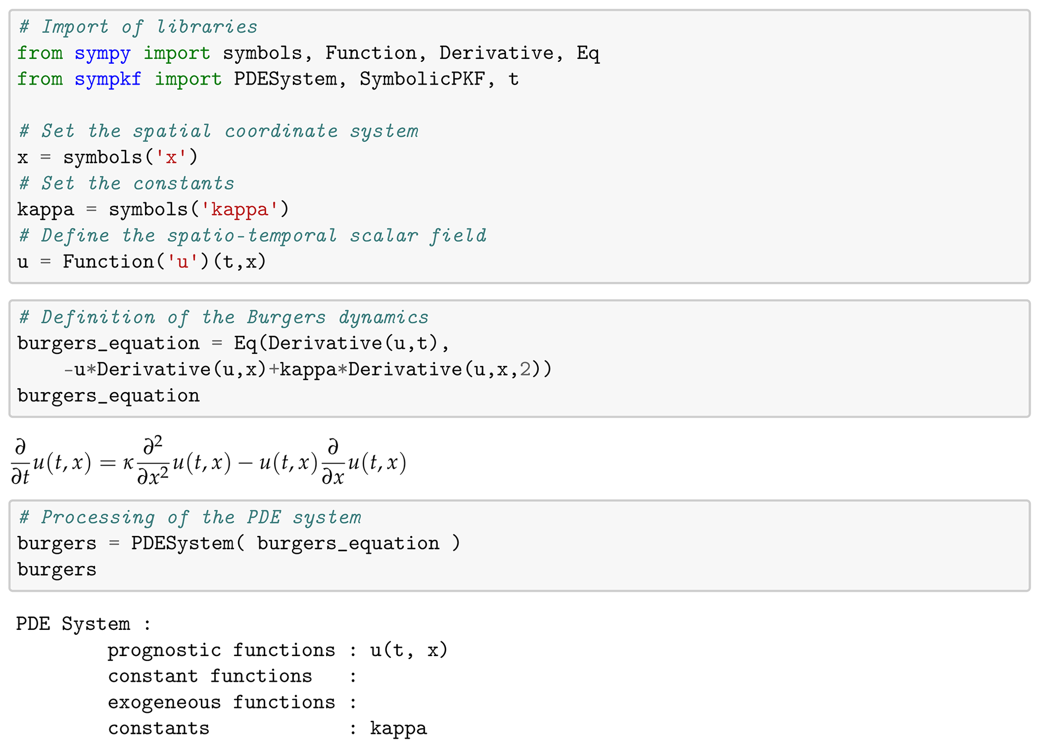
Figure 1 Sample of code and Jupyter notebook outputs for the definition of the Burgers dynamics using SymPKF.

In this example, the dynamics consist of a single equation defined as an instance of the class Eq, but in the general situation in which the dynamics are given as a system of equations, the dynamics have to be represented as a Python list of equations.

A preprocessing of the dynamics is then performed to determine several important quantities to handle the dynamics: the prognostic fields (functions for which a time derivative is present), the diagnostic fields (functions for which there is no time derivative in the dynamics), the constant functions (functions that only depend on the spatial coordinates), and the constants (pure scalar terms that are not a function of any coordinate). This preprocessing is performed when transforming the dynamics as an instance of the class PDESystem and whose default string output delivers a summary of the dynamics: for the Burgers equation, there is only one prognostic function, u(t,x), and one constant, κ.

The prognostic quantities being known, it is then possible to perform the computation of the PKF dynamics, as discussed now.

4.2 Computation of the VLATcov PKF dynamics

Thanks to the preprocessing, we are able to determine the VLATcov parameters needed to compute the PKF dynamics, which are the variance and the anisotropy tensor associated with the prognostic fields. For the Burgers equation, the VLATcov parameters are the variance V_u and the metric tensor ${\mathbf{g}}_u=\left(g_{u,xx}\right)$ or its associated aspect tensor ${\mathbf{s}}_u=\left(s_{u,xx}\right)$. Note that, in SymPKF, the VLATcov parameters are labeled by their corresponding prognostic fields to facilitate their identification. This labeling is achieved when the dynamics are transformed as an instance of the class SymbolicPKF. This class is at the core of the computation of the PKF dynamics from Eq. (16).

As discussed in Sect. 2.2.1, the PKF dynamics rely on the second-order fluctuation–mean interaction dynamics wherein each prognostic function is replaced by a stochastic counterpart. Hence, the constructor of SymbolicPKF converts each prognostic function as a function of an additional coordinate, ω∈Ω. For the Burgers equation, u(t,x) becomes $u(t,x,\mathit{\omega })$.

Since the computation of the second-order fluctuation–mean interaction dynamics relies on the expectation operator, an implementation of this expectation operator has been introduced in SymPKF: it is defined as the class Expectation built by inheritance from the class sympy.Function to leverage the computational facilities of SymPy. The implementation of the class Expectation is based on the linearity of the mathematical expectation operator with respect to deterministic quantities and its commutativity with partial derivatives and integrals with respect to coordinates different from ω, e.g., for the Burgers equation $\mathbb{E}\left[{\partial }_{x}u\right(t,x,\mathit{\omega }\left)\right]={\partial }_x\mathbb{E}\left[u\right(t,x,\mathit{\omega }\left)\right]$. Note that $\mathbb{E}\left[u\right(t,x,\mathit{\omega }\left)\right]$ is a function of (t,x) only: the expectation operator converts a random variable into a deterministic variable.

Then, the symbolic computation of the second-order fluctuation–mean interaction dynamics in Eq. (16a) is performed, thanks to SymPy, by following the steps as described in Sect. 2.2.1. In particular, the computation also leads to the tangent-linear dynamics of the error in Eq. (6), from which it is possible to compute the dynamics of the variance in Eq. (16b) and of the metric tensor in Eq. (16c) (or its associated aspect tensor version). Applying these steps and the appropriate substitutions, this is achieved when calling the in_metric or in_aspect Python property of an instance of the class SymbolicPKF. This is shown for the Burgers equation in Fig. 2, where the background computation of the PKF dynamics leads to a list of the three coupled equations corresponding to the mean, the variance, and the aspect tensor, similar to the system in Eq. (22) first obtained by Pannekoucke et al. (2018a).

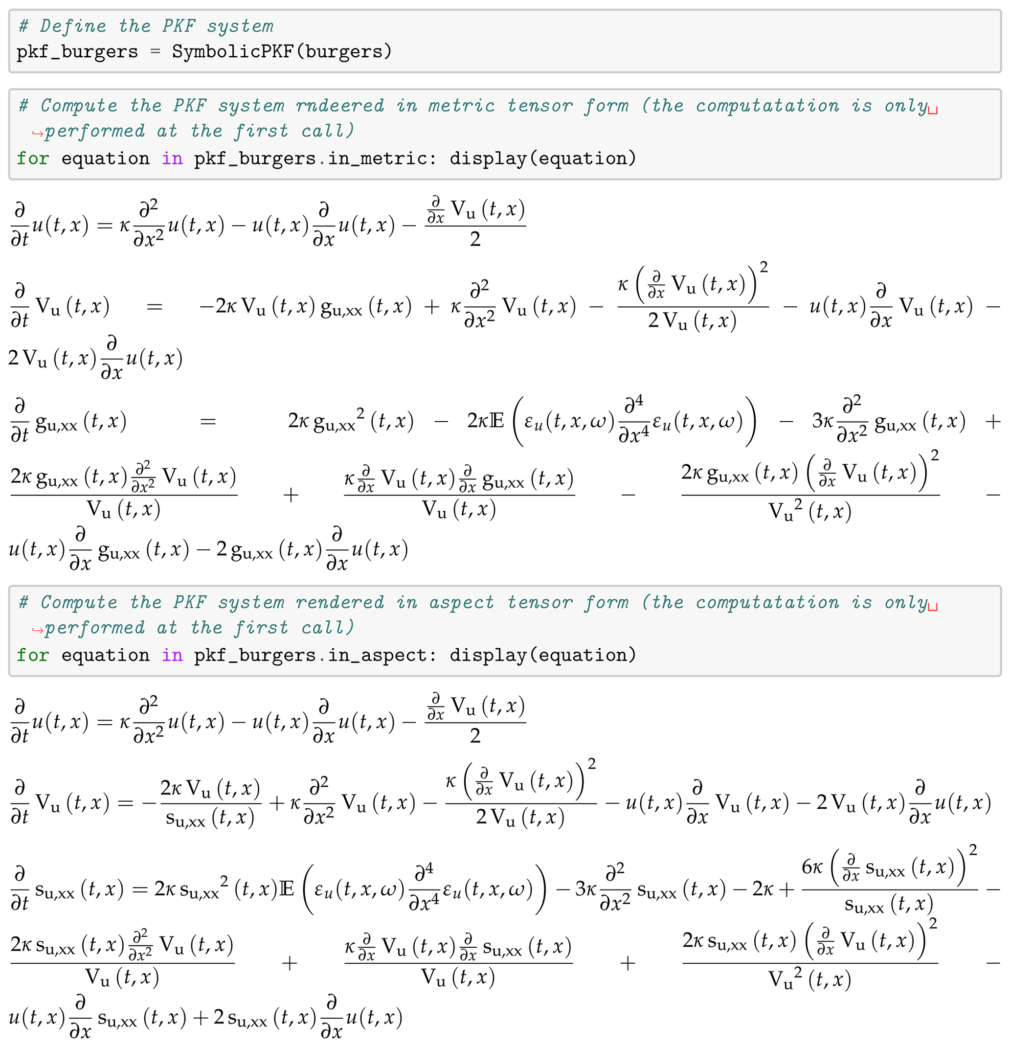
Figure 2 Sample of code and Jupyter notebook outputs: systems of partial differential equations given in metric and in aspect forms produced by SymPKF when applied to the Burgers equation (Eq. 20).

Hence, from SymPKF, for the Burgers equation, the VLATcov PKF dynamics given in the aspect tensor read as

$$\begin{array}{}\text{(21)}& \left\{\begin{array}{lll}{\partial }_{\mathrm{t}}u& =& \mathit{\kappa }{\partial }_x^{\mathrm{2}}u-u{\partial }_{x}u-\frac{{\partial }_x{V}_u}{\mathrm{2}}\\ {\partial }_{\mathrm{t}}{V}_u& =& -\frac{\mathrm{2}\mathit{\kappa }{V}_u}{s_{u,xx}}+\mathit{\kappa }{\partial }_x^{\mathrm{2}}{V}_u-\frac{\mathit{\kappa }{\left({\partial }_x{V}_u\right)}^{\mathrm{2}}}{\mathrm{2}{V}_u}\\ & & -u{\partial }_x{V}_u-\mathrm{2}{V}_u{\partial }_{x}u\\ {\partial }_{\mathrm{t}}{s}_{u,xx}& =& \mathrm{2}\mathit{\kappa }{s}_{u,xx}^{\mathrm{2}}\mathbb{E}\left({\mathit{\epsilon }}_u{\partial }_x^{\mathrm{4}}{\mathit{\epsilon }}_u\right)-\mathrm{3}\mathit{\kappa }{\partial }_x^{\mathrm{2}}{s}_{u,xx}\\ & & -\mathrm{2}\mathit{\kappa }+\frac{\mathrm{6}\mathit{\kappa }{\left({\partial }_x{s}_{u,xx}\right)}^{\mathrm{2}}}{s_{u,xx}}-\frac{\mathrm{2}\mathit{\kappa }{s}_{u,xx}{\partial }_x^{\mathrm{2}}{V}_u}{V_u}\\ & & +\frac{\mathit{\kappa }{\partial }_x{V}_u{\partial }_x{s}_{u,xx}}{V_u}+\frac{\mathrm{2}\mathit{\kappa }{s}_{u,xx}{\left({\partial }_x{V}_u\right)}^{\mathrm{2}}}{V_u^{\mathrm{2}}}\\ & & -u{\partial }_x{s}_{u,xx}+\mathrm{2}{s}_{u,xx}{\partial }_{x}u\end{array}\right.,\end{array}$$

where s_u,xx is the single component of the aspect tensor s_u in 1D domains. Note that in the output of the PKF equations, as reproduced in Eq. (21), the expectation in the dynamics of the mean is replaced by the prognostic field; for the Burgers equation, 𝔼[u](t,x) is simply denoted by u(t,x).

While the Burgers equation only contains two physical processes, i.e., the nonlinear advection and the diffusion, the resulting PKF dynamics in Eq. (21) make numerous terms appear, which justifies the use of symbolic computation, as mentioned above. The computation of the PKF dynamics leading to the metric and to the aspect tensor formulation takes about 1 s of computation (Intel Core i7-7820HQ CPU at 2.90 GHz × 8).

In this example, the splitting strategy has not been considered to simplify the computation of the PKF dynamics. However, it can be done by considering the PKF dynamics for the advection ${\partial }_{\mathrm{t}}u=-u{\partial }_{x}u$ and the diffusion ${\partial }_{\mathrm{t}}u=\mathit{\kappa }{\partial }_x^{\mathrm{2}}u$, and computed separately, then merged to find the PKF dynamics of the full Burgers equation. For instance, Fig. 3 shows the PKF dynamics for the advection (first cell) and for the diffusion (second cell); the output can be traced back in Eq. (2), e.g., by the terms in κ for the diffusion.

Figure 3 Illustration of the splitting strategy that can be used to compute the PKF dynamics and applied here for the Burgers equation: PKF dynamics of the Burgers equation can be obtained from the PKF dynamics of the advection (first cell) and of the diffusion (second cell).

Thanks to the symbolic computation using the expectation operator, as implemented by the class Expectation, it is possible to handle terms such as $\mathbb{E}\left[{\mathit{\epsilon }}_u{\partial }_x^{\mathrm{4}}{\mathit{\epsilon }}_u\right]$ during the computation of the PKF dynamics. The next section details how these terms are handled during the computation and the closure issue they bring.

4.3 Comments on the computation of the VLATcov PKF dynamics and the closure issue

4.3.1 Computation of terms $\mathbb{E}\left[{\partial }^{\mathit{\alpha }}\mathit{\epsilon }{\partial }^{\mathit{\beta }}\mathit{\epsilon }\right]$ and their connection to the correlation function

An important point is that terms such as 𝔼[ε∂^αε], e.g., $\mathbb{E}\left[{\mathit{\epsilon }}_u{\partial }_x^{\mathrm{4}}{\mathit{\epsilon }}_u\right]$ in Eq. (21) are directly connected to the correlation function $\mathit{\rho }(\mathbf{x},\mathbf{y})=\mathbb{E}\left[\mathit{\epsilon }\right(\mathbf{x}\left)\mathit{\epsilon }\right(\mathbf{y}\left)\right]$ whose Taylor expansion is written as

$$\begin{array}{}\text{(22)}& \mathit{\rho }(\mathbf{x},\mathbf{x}+\mathit{\delta }\mathbf{x})=\sum _k{\displaystyle \frac{\mathrm{1}}{k\mathrm{!}}}\mathbb{E}\left[\mathit{\epsilon }\left(\mathbf{x}\right){\partial }^k\mathit{\epsilon }\left(\mathbf{x}\right)\right]\mathit{\delta }{\mathbf{x}}^k.\end{array}$$

However, during their computation, the VLATcov PKF dynamics make the terms $\mathbb{E}\left[{\partial }^{\mathit{\alpha }}\mathit{\epsilon }{\partial }^{\mathit{\beta }}\mathit{\epsilon }\right]$ appear, with $\left|\mathit{\alpha }\right|\le \left|\mathit{\beta }\right|$, where for any α, ∂^α denotes the derivative with respect to the multi-index $\mathit{\alpha }=({\mathit{\alpha }}_i{)}_{i\in [\mathrm{1},n]}$, with α_i denoting the derivative order with respect to the ith coordinate x_i of the coordinate system and where the sum of all derivative order is denoted by $\left|\mathit{\alpha }\right|={\sum }_i{\mathit{\alpha }}_i$. The issue it that these terms in $\mathbb{E}\left[{\partial }^{\mathit{\alpha }}\mathit{\epsilon }{\partial }^{\mathit{\beta }}\mathit{\epsilon }\right]$ are not directly connected to the Taylor expansion in Eq. (22).

The interesting property of these terms is that they can be reworded as spatial derivatives of terms in the form 𝔼[ε∂^γε]. More precisely, any term $\mathbb{E}\left[{\partial }^{\mathit{\alpha }}\mathit{\epsilon }{\partial }^{\mathit{\beta }}\mathit{\epsilon }\right]$ can be written from derivative of terms in 𝔼[ε∂^γε], where $\left|\mathit{\gamma }\right|<\left|\mathit{\alpha }\right|+\left|\mathit{\beta }\right|$, and the term $\mathbb{E}\left[\mathit{\epsilon }{\partial }^{\mathit{\alpha }+\mathit{\beta }}\mathit{\epsilon }\right]$ (see Appendix B for the proof). So, to replace any term in $\mathbb{E}\left[{\partial }^{\mathit{\alpha }}\mathit{\epsilon }{\partial }^{\mathit{\beta }}\mathit{\epsilon }\right]$ by terms in 𝔼[ε∂^γε], where $\left|\mathit{\gamma }\right|<\left|\mathit{\alpha }\right|+\left|\mathit{\beta }\right|$, a substitution dictionary is computed in SymPKF and stored as the variable subs_tree. The computation of this substitution dictionary is performed thanks to a dynamical programming strategy. Thereafter, the integer $\left|\mathit{\alpha }\right|+\left|\mathit{\beta }\right|$ is called the order of the term $\mathbb{E}\left[{\partial }^{\mathit{\alpha }}\mathit{\epsilon }{\partial }^{\mathit{\beta }}\mathit{\epsilon }\right]$. Figure 4 shows the substitution dictionary computed for the Burgers equation. It appears that terms of order lower than 3 can be explicitly written from the metric (or its derivatives), while terms of order larger than 4 cannot: this is known as the closure issue (Pannekoucke et al., 2018a).

Figure 4 Substitution dictionary computed in SymPKF to replace terms such as $\mathbb{E}\left[{\partial }^{\mathit{\alpha }}\mathit{\epsilon }{\partial }^{\mathit{\beta }}\mathit{\epsilon }\right]$ by terms in 𝔼[ε∂^γε], where $\left|\mathit{\gamma }\right|<\left|\mathit{\alpha }\right|+\left|\mathit{\beta }\right|$.

The term $\mathbb{E}\left[\mathit{\epsilon }{\partial }_x^{\mathrm{4}}\mathit{\epsilon }\right]$, which features long-range correlations, cannot be related to the variance or to the metric and has to be closed. We detail this point in the next section.

4.3.2 Analytical and data-driven closure

A naïve closure for the PKF dynamics in Eq. (21) would be to replace the unknown term $\mathbb{E}\left[{\mathit{\epsilon }}_u{\partial }_x^{\mathrm{4}}{\mathit{\epsilon }}_u\right]$ by zero. However, in the third equation that corresponds to the aspect tensor dynamics, the coefficient −3κ of the diffusion term ${\partial }_x^{\mathrm{2}}{s}_u$ being negative, it follows that the dynamics of s_u numerically explode at an exponential rate. Of course, because the system represents the uncertainty dynamics of the Burgers equation in Eq. (20) that is well posed, the parametric dynamics should not explode. Hence, the unknown term $\mathbb{E}\left[{\mathit{\epsilon }}_u{\partial }_x^{\mathrm{4}}{\mathit{\epsilon }}_u\right]$ is crucial: it can balance the negative diffusion to stabilize the parametric dynamics.

For the Burgers equation, a closure for $\mathbb{E}\left[{\mathit{\epsilon }}_u{\partial }_x^{\mathrm{4}}{\mathit{\epsilon }}_u\right]$ has been previously proposed (Pannekoucke et al., 2018a), given by

$$\begin{array}{}\text{(23)}& \mathbb{E}\left[{\mathit{\epsilon }}_u{\partial }_x^{\mathrm{4}}{\mathit{\epsilon }}_u\right]\sim {\displaystyle \frac{\mathrm{2}}{s_u^{\mathrm{2}}}}{\partial }_x^{\mathrm{2}}{s}_u+{\displaystyle \frac{\mathrm{3}}{s_u^{\mathrm{2}}}}-\mathrm{4}{\displaystyle \frac{{\left({\partial }_x{s}_u\right)}^{\mathrm{2}}}{s_u^{\mathrm{3}}}},\end{array}$$

where the symbol ∼ is used to indicate that this is not an equality but a proposal of closure for the term in the left-hand side and that leads to the closed system

$$\begin{array}{}\text{(24)}& \left\{\begin{array}{ccl}{\partial }_{\mathrm{t}}u& =& -u{\partial }_{x}u+\mathit{\kappa }{\partial }_x^{\mathrm{2}}u-\frac{\mathrm{1}}{\mathrm{2}}{\partial }_x{V}_u,\\ {\partial }_{\mathrm{t}}{V}_u& =& -u{\partial }_x{V}_u-\mathrm{2}\left({\partial }_{x}u\right)V_u+\mathit{\kappa }{\partial }_x^{\mathrm{2}}{V}_u\\ & & -\frac{\mathit{\kappa }}{\mathrm{2}}\frac{\mathrm{1}}{V_u}({\partial }_x{V}_u{)}^{\mathrm{2}}-\frac{\mathrm{2}\mathit{\kappa }}{s_{u,xx}}{V}_u,\\ {\partial }_{\mathrm{t}}{s}_{u,xx}& =& -u{\partial }_x{s}_{u,xx}+\mathrm{2}\left({\partial }_{x}u\right)s_{u,xx}+\mathrm{4}\mathit{\kappa }\\ & & -\mathrm{2}\frac{\mathit{\kappa }{s}_{u,xx}}{V_u}{\partial }_x^{\mathrm{2}}{V}_u+\mathrm{2}\frac{\mathit{\kappa }{s}_{u,xx}}{V_u^{\mathrm{2}}}({\partial }_x{V}_u{)}^{\mathrm{2}}\\ & & +\mathit{\kappa }\frac{\mathrm{1}}{V_u}{\partial }_x{V}_u{\partial }_x{s}_{u,xx}+\mathit{\kappa }{\partial }_x^{\mathrm{2}}{s}_{u,xx}\\ & & -\mathrm{2}\mathit{\kappa }\frac{\mathrm{1}}{s_{u,xx}}({\partial }_x{s}_{u,xx}{)}^{\mathrm{2}}.\end{array}\right.\end{array}$$

The closure in Eq. (23) results from a local Gaussian approximation of the correlation function. Previous numerical experiments have shown that this closure is well adapted to the Burgers equation (Pannekoucke et al., 2018a). But the approach that has been followed to find this closure is quite specific, and it would be interesting to design a general way to find such a closure.

In particular, it would be interesting to search for a generic way to design closures that leverage the symbolic computation, which could be plugged with the PKF dynamics computed from SymPKF at a symbolic level. To do so, we propose an empirical closure that leverages a data-driven strategy to hybridize machine learning with physics, as proposed by Pannekoucke and Fablet (2020) with their neural network generator PDE-NetGen.

The construction of the proposal relies on the symbolic computation shown in Fig. 5.

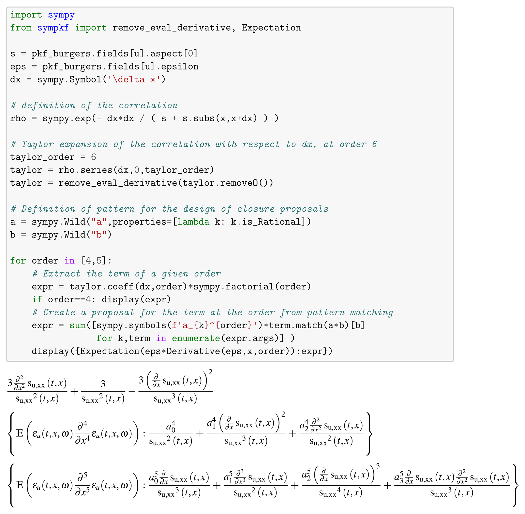
Figure 5 Example of a symbolic computation leading to a proposal for the closure of the unknown terms of order 4 and 5.

The first step is to consider an analytical approximation for the correlation function. For the illustration, we consider the local correlation function to be well approximated by the quasi-Gaussian function

$$\begin{array}{}\text{(25)}& \mathit{\rho }(x,x+\mathit{\delta }x)\approx \exp \left(-{\displaystyle \frac{\mathit{\delta }{x}^{\mathrm{2}}}{s_u\left(x\right)+s_u(x+\mathit{\delta }x)}}\right).\end{array}$$

Then, the second step is to perform the computation of the Taylor's expansion of Eq. (22) at a symbolic level. This is done thanks to SymPy with the method series applied to Eq. (25) for δx near the value 0 and at a given order; e.g., for the illustration expansion is computed as the sixth order in Fig. 5.

Then, the identification with the Taylor's expansion in Eq. (22) leads to the closure

$$\begin{array}{}\text{(26)}& \mathbb{E}\left[{\mathit{\epsilon }}_u{\partial }_x^{\mathrm{4}}{\mathit{\epsilon }}_u\right]\sim {\displaystyle \frac{\mathrm{3}}{s_{u,xx}^{\mathrm{2}}}}{\partial }_x^{\mathrm{2}}{s}_{u,xx}+{\displaystyle \frac{\mathrm{3}}{s_{u,xx}^{\mathrm{2}}}}-\mathrm{3}{\displaystyle \frac{{\left({\partial }_x{s}_{u,xx}\right)}^{\mathrm{2}}}{s_{u,xx}^{\mathrm{3}}}}.\end{array}$$

While it looks like the closure in Eq. (23), the coefficients are not the same. But this suggests that the closure of $\mathbb{E}\left[{\mathit{\epsilon }}_u{\partial }_x^{\mathrm{4}}{\mathit{\epsilon }}_u\right]$ can be expanded as

$$\begin{array}{}\text{(27)}& \mathbb{E}\left[{\mathit{\epsilon }}_u{\partial }_x^{\mathrm{4}}{\mathit{\epsilon }}_u\right]\sim {\displaystyle \frac{a_{\mathrm{0}}^{\mathrm{4}}}{s_{u,xx}^{\mathrm{2}}}}{\partial }_x^{\mathrm{2}}{s}_{u,xx}+{\displaystyle \frac{a_{\mathrm{1}}^{\mathrm{4}}}{s_{u,xx}^{\mathrm{2}}}}+a_{\mathrm{3}}^{\mathrm{4}}{\displaystyle \frac{{\left({\partial }_x{s}_{u,xx}\right)}^{\mathrm{2}}}{s_{u,xx}^{\mathrm{3}}}},\end{array}$$

where ${\mathbf{a}}^{\mathrm{4}}=(a_{\mathrm{0}}^{\mathrm{4}},a_{\mathrm{1}}^{\mathrm{4}},a_{\mathrm{2}}^{\mathrm{4}})$ represents three unknown reals. A data-driven strategy can be considered to find an appropriate value of a⁴ from experiments. This has been investigated by using the automatic generator of a neural network PDE-NetGen, which bridges the gap between the physics and the machine learning (Pannekoucke and Fablet, 2020) and with which the training has led to the value ${\mathbf{a}}^{\mathrm{4}}\approx (\mathrm{1.86},\mathrm{3.0},\mathrm{-}\mathrm{3.6})$. Since this proposal is deduced from symbolic computation, it is easy to build some proposals for higher-order unknown terms as is shown in Fig. 5 for the term $\mathbb{E}\left[{\mathit{\epsilon }}_u{\partial }_x^{\mathrm{5}}{\mathit{\epsilon }}_u\right]$.

Whatever closure has been obtained in an analytical or an empirical way, it remains to compute the closed PKF dynamics to assess their performance. To do so a numerical implementation of the system of partial differential equations has to be introduced. As for the computation of the PKF dynamics, the design of a numerical code can be tedious, with a risk of introducing errors in the implementation due to the numerous terms occurring in the PKF dynamics. To facilitate the research on the PKF, SymPKF comes with a Python numerical code generator, which provides an end-to-end investigation of the PKF dynamics. This code generator is now detailed.

Figure 6 Introduction of a closure and automatic generation of a numerical code in SymPKF.

4.4 Automatic code generation for numerical simulations

While compiled language with appropriate optimization should be important for industrial applications, we chose to implement a pure Python code generator, which offers a simple research framework for exploring the design of PKF dynamics. It would have been possible to use a code generator already based on SymPy (see, e.g., Louboutin et al., 2019), but with such code generators being domain-specific, it was less adapted to the investigation of the PKF for arbitrary dynamics. Instead, we consider a finite-difference implementation of partial derivatives with respect to spatial coordinates. The default domain to perform the computation is the periodic unit square with the dimension of the number of spatial coordinates. The length of the domain can be specified along each direction. The domain is regularly discretized along each direction, while the number of grid points can be specified for each direction.

The finite difference takes the form of an operator ℱ that approximates any partial derivate at a second order of consistency: for any multi-index α, ${\mathcal{F}}^{\mathit{\alpha }}u\underset{0}{=}{\partial }^{\mathit{\alpha }}u+\mathcal{O}\left(\right|\mathit{\delta }\mathbf{\text{x}}{|}^{\mathrm{2}})$, where 𝒪 is Landau's big O notation. For any f, the notation $f\left(\mathit{\delta }x\right)\underset{0}{=}\mathcal{O}\left(\mathit{\delta }{x}^{\mathrm{2}}\right)$ means that ${lim}_{\mathit{\delta }x\to \mathrm{0}}\frac{f\left(\mathit{\delta }x\right)}{\mathit{\delta }{x}^{\mathrm{2}}}$ is finite. The operator ℱ computed with respect to independent coordinates commutes, e.g., ${\mathcal{F}}_{xy}={\mathcal{F}}_x\circ {\mathcal{F}}_y={\mathcal{F}}_y\circ {\mathcal{F}}_x$, where ∘ denotes the composition, but it does not commute for dependent coordinates, e.g., ${\mathcal{F}}_x^{\mathrm{2}}\ne {\mathcal{F}}_x\circ {\mathcal{F}}_x$. The finite difference of the partial derivative with respect to the multi-index is computed sequentially, e.g., ${\mathcal{F}}_{xxy}={\mathcal{F}}_x^{\mathrm{2}}\circ {\mathcal{F}}_y={\mathcal{F}}_y\circ {\mathcal{F}}_x^{\mathrm{2}}$. The finite difference of order α with respect to a single spatial coordinate is the centered finite difference based on α+1 points.

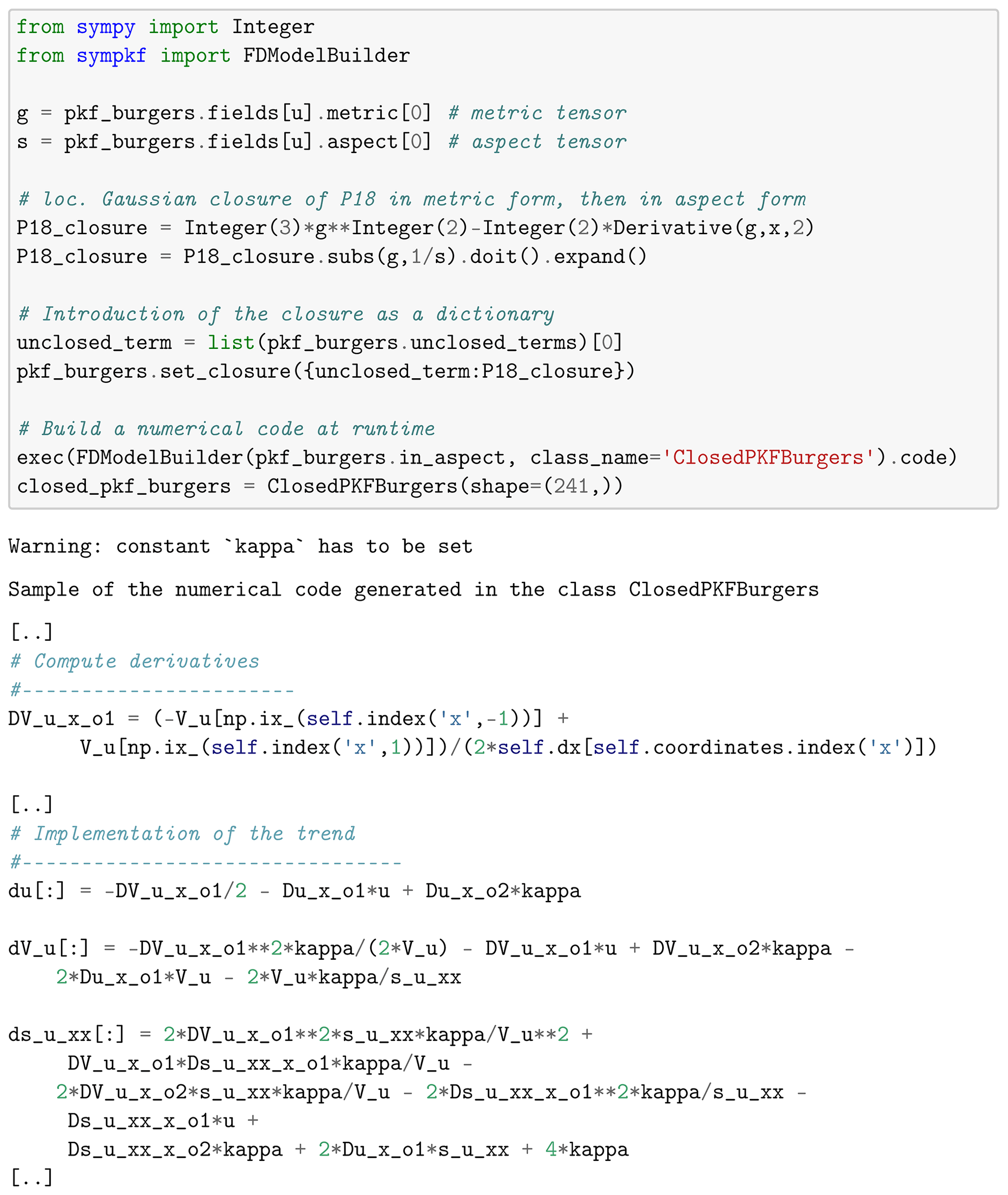
For instance, Fig. 6 shows how to close the PKF dynamics for the Burgers equation following P18 and how to build a code from an instance of the class sympkf.FDModelBuilder: it creates the class ClosedPKFBurgers. In this example, the code is rendered from templates thanks to Jinja³; then it is executed at runtime. Note that the code can also be written in an appropriate Python module for adapting the code to a particular situation or to check the correctness of the generated code. At the end, the instance closed_pkf_burgers of the class ClosedPKFBurgers is created, raising a warning to indicate that the value of constant κ has to be specified before performing a numerical simulation. Note that it is possible to set the value of kappa as a keyword argument in the class ClosedPKFBurgers. Figure 6 also shows a sample of the generated code with the implementation of the computation of the first-order partial derivative ∂_xV_u, which appears as a centered finite difference. Then, the sample of code shows how the partial derivatives are used to compute the trend of the system of partial differential equations in Eq. (24).

The numerical integration is handled through the inheritance mechanism: the class ClosedPKFBurgers inherits the integration time loop from the class sympkf.Model as described by the unified modeling language (UML) diagram shown in Fig. 7. In particular, the class Model contains several time schemes, e.g., a fourth-order Runge–Kutta scheme. Note that in the present implementation of SymPKF, only explicit time schemes are considered, but it could be possible to leverage the symbolic computation to implement other schemes more adapted to a given PDE, e.g., an implicit scheme for the transport or the diffusion or a high-order exponential time-differencing method (Kassam and Trefethen, 2005) with which the linear and the nonlinear parts would be automatically determined from the symbolic computation. The details of the instance closed_pkf_burgers of the class ClosedPKFBurgers make it appear that the closed system in Eq. (24) will be integrated by using a RK4 time scheme on the segment [0,D] (here D=1) with periodic boundaries and discretized by 241 points.

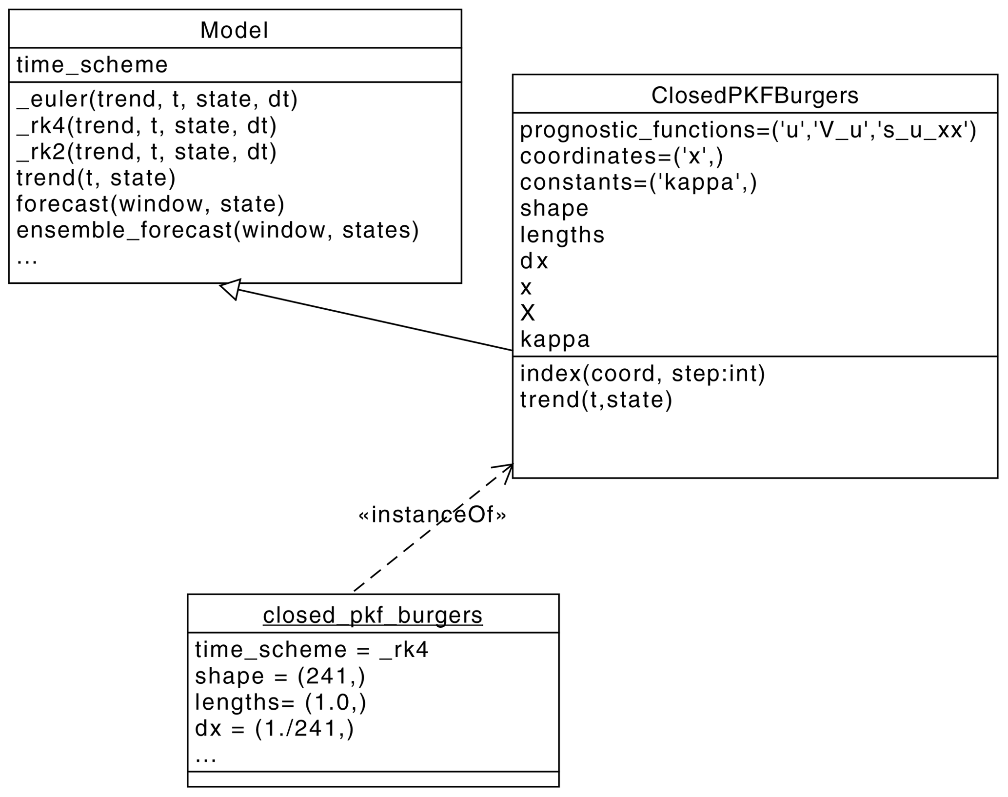
Figure 7 UML diagram showing the inheritance mechanism implemented in SymPKF: the class ClosedPKFBurgers inherits from the class Model, which implements several time schemes. Here, closed_pkf_burgers is an instance of the class ClosedPKFBurgers.

Thanks to the end-to-end framework proposed in SymPKF, it is possible to perform a numerical simulation based on the PKF dynamics in Eq. (23). To do so, we set κ=0.0025 and consider the simulation starting from the Gaussian distribution $\mathcal{N}(u_{\mathrm{0}},{\mathbf{P}}_h^{\mathrm{f}})$ of mean $u_{\mathrm{0}}\left(x\right)=U_{\max }[\mathrm{1}+\cos (\mathrm{2}\mathit{\pi }(x-D/\mathrm{4})/D\left)\right]/\mathrm{2}$ with U_max=0.5 and of covariance matrix

$$\begin{array}{}\text{(28)}& {\mathbf{P}}_h^{\mathrm{f}}(x,y)=V_h\exp \left(-{\displaystyle \frac{(x-y{)}^{\mathrm{2}}}{\mathrm{2}{l}_h^{\mathrm{2}}}}\right),\end{array}$$

where V_h=0.01U_max and $l_h=\mathrm{0.02}D\approx \mathrm{5}\mathrm{d}x$. The time step of the fourth-order Runge–Kutta scheme is dt=0.002. The evolution predicted from the PKF is shown in Fig. 8 (solid lines). This simulation illustrates the time evolution of the mean (panel a) and of the variance (panel b); panel (c) represents the evolution of the correlation length scale defined from the aspect tensor as $L\left(x\right)=\sqrt{s_{u,xx}\left(x\right)}$. Note that at time 0, the length scale field is L(x)=l_h. For the illustrations, the variance (the length scale) is normalized by its initial value V_h (l_h).

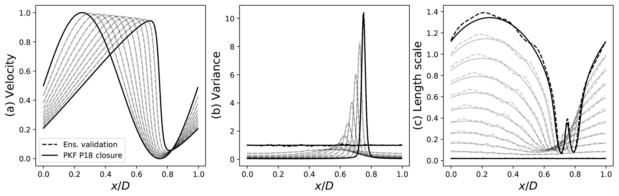
Figure 8 Illustration of a numerical simulation of the PKF dynamics in Eq. (23) (solid line), with the mean (a), the variance (b), and the correlation length scale (c), which is defined from the component s_u,xx of the aspect tensor by $L\left(x\right)=\sqrt{s_{u,xx}\left(x\right)}$. An ensemble-based validation of the PKF dynamics is shown as a dashed line. (Pannekoucke and Fablet, 2020, see their Fig. 7)

In order to show the skill of the PKF applied to the Burgers equation, when using the closure of P18, an ensemble validation is now performed. Note that the code generator of SymPKF can be used for arbitrary dynamics, e.g., the Burgers equation itself. Hence, a numerical code solving the Burgers equation is rendered from its symbolic definition. Then an ensemble of 1600 forecasts is computed starting from an ensemble of initial errors at time 0. The ensemble of initial errors is sampled from the Gaussian distribution $\mathcal{N}\left(\mathrm{0},{\mathbf{P}}_h^{\mathrm{f}}\right)$ of zero mean and covariance matrix ${\mathbf{P}}_h^{\mathrm{f}}$. Note that the ensemble forecasting implemented in SymPKF as the method Model.ensemble_forecast (see Fig. 7) leverages the multiprocessing tools of Python to use the multiple cores of the CPU when present. On the computer used for the simulation, the forecasts are performed in parallel on eight cores. The ensemble estimation of the mean, the variance, and the length scale is shown in Fig. 8 (dashed lines). Since the ensemble is finite, sampling noise is visible, e.g., in the variance at the initial time that is not strictly equal to V_h. In this simulation, it appears that the PKF (solid line) coincides with the ensemble estimation (dashed lines), which shows the ability of the PKF to predict the forecast error covariance dynamics. Note that the notebook corresponding to the Burgers experiment is available in the example directory of SymPKF.

While this example shows an illustration of SymPKF in a 1D domain, the package also applies in 2D and 3D domains, as presented now.

4.5 Illustration of dynamics in a 2D domain

In order to illustrate the ability of SymPKF to apply in a 2D or 3D domain, we consider the linear advection of a scalar field $c(t,x,y)$ by a stationary velocity field $\mathbf{u}=\left(u\right(x,y),v(x,y\left)\right)$, which reads as the partial differential equation

$$\begin{array}{}\text{(29)}& {\partial }_{\mathrm{t}}c+\mathbf{u}\mathrm{\nabla }c=\mathrm{0}.\end{array}$$

As for the Burgers equation, the definition of the dynamics relies on SymPy (not shown but similar to the definition of the Burgers equation as given in Fig. 1). This leads to preprocessing the dynamics by creating the instance advection of the class PDESystem, which transforms the equation into a system of partial differential equations. In particular, the procedure will diagnose the prognostic functions of dynamics, here the function c. Then it identifies the constant functions, which can depend on space but not on time: here, these are the components of the velocity (u, v). The process also identifies exogenous functions and constants, of which there are none here.

The calculation of the parametric dynamics is handled by the class SymbolicPKF as shown in the first cell in Fig. 9. The parametric dynamics are a property of the instance pkf_advection of the class SymbolicPKF, and when it is called, the parametric dynamics are computed once and for all. The parametric dynamics formulated in terms of metric are first computed; see the second cell. For the 2D linear advection, the parametric dynamics are a system of five partial differential equations, as is shown in the output of the second cell: the dynamics of the ensemble average 𝔼[c], which outputs as c for the sake of simplicity (first equation), the dynamics of the variance (second equation), and the dynamics of the local metric tensor (last three equations). In compact form, the dynamics are given by the system

$$\begin{array}{}\text{(30a)}& {\displaystyle }& {\displaystyle }{\partial }_{\mathrm{t}}c+\mathbf{u}\mathrm{\nabla }c=\mathrm{0},\text{(30b)}& {\displaystyle }& {\displaystyle }{\partial }_{\mathrm{t}}{V}_c+\mathbf{u}\mathrm{\nabla }{V}_c=\mathrm{0},\text{(30c)}& {\displaystyle }& {\displaystyle }{\partial }_{\mathrm{t}}{\mathbf{g}}_c+\mathbf{u}\mathrm{\nabla }{\mathbf{g}}_c=-{\mathbf{g}}_c\left(\mathrm{\nabla }\mathbf{u}\right)-{\left(\mathrm{\nabla }\mathbf{u}\right)}^{\mathrm{T}}{\mathbf{g}}_c,\end{array}$$

which corresponds to the 2D extension of the 1D dynamics first found by Cohn (1993) (Pannekoucke et al., 2016) and validates the computation performed in SymPKF. Due to the linearity of the linear advection in Eq. (29), the ensemble average in Eq. (30a) is governed by the same dynamics as in Eq. (29). While both the variance in Eq. (30b) and the metric are advected by the flow, the metric is also deformed by the shear in Eq. (30c). This deformation more commonly appears in the dynamics written in aspect tensor form, which is given by

$$\begin{array}{}\text{(31a)}& {\displaystyle }& {\displaystyle }{\partial }_{\mathrm{t}}c+\mathbf{u}\mathrm{\nabla }c=\mathrm{0},\text{(31b)}& {\displaystyle }& {\displaystyle }{\partial }_{\mathrm{t}}{V}_c+\mathbf{u}\mathrm{\nabla }{V}_c=\mathrm{0},\text{(31c)}& {\displaystyle }& {\displaystyle }{\partial }_{\mathrm{t}}{\mathbf{s}}_c+\mathbf{u}\mathrm{\nabla }{\mathbf{s}}_c=\left(\mathrm{\nabla }\mathbf{u}\right){\mathbf{s}}_c+{\mathbf{s}}_c{\left(\mathrm{\nabla }\mathbf{u}\right)}^T,\end{array}$$

where Eq. (31c) is similar to the dynamics of the conformation tensor in viscoelastic flow (Bird and Wiest, 1995; Hameduddin et al., 2018).

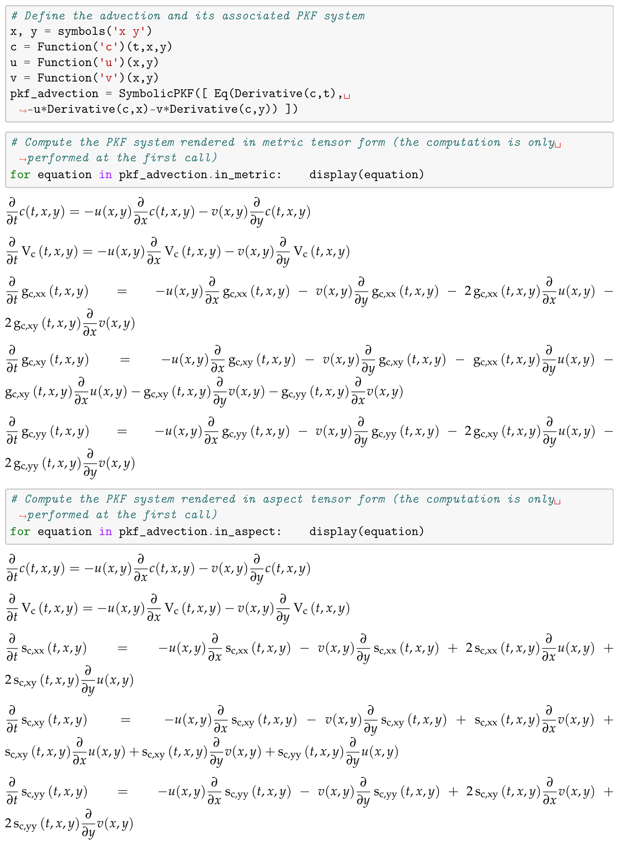
Figure 9 Sample of code and Jupyter notebook outputs: system of partial differential equations produced by SymPKF when applied to the linear advection in Eq. (29).

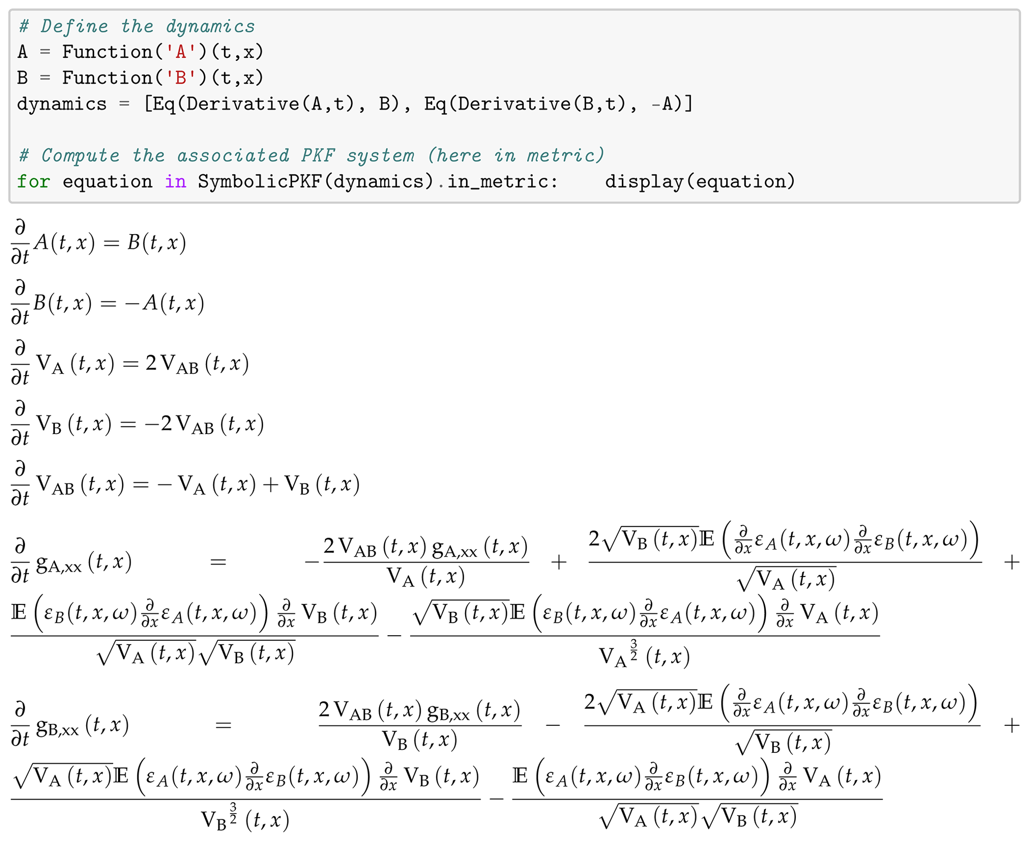
Figure 10 Output of the computation by SymPKF of the PKF dynamics for the simple multivariate periodic chemical reaction, corresponding to the right-hand side of Eq. (32).

We do not introduce any numerical simulation of the PKF dynamics in Eq. (30) or Eq. (31), but interested readers are referred to the 2D numerical PKF assimilation cycles of Pannekoucke (2021b), which have been made thanks to SymPKF.

This example illustrates a 2D situation and shows the multidimensional capabilities of SymPKF. Similarly to the simulation conducted for the Burgers equation, it is possible to automatically generate a numerical code able to perform numerical simulations of the dynamics in Eq. (31) (not shown here). Hence, this 2D domain example showed the ability of SymPKF to apply in dimensions larger than 1D.

Before concluding, we would like to present a preliminary application of SymPKF in a multivariate situation.

4.6 Towards the PKF for multivariate dynamics

SymPKF can be used to compute the prediction of the variance and the anisotropy in a multivariate situation.

Note that one of the difficulties with the multivariate situation is that the number of equations increases linearly with the number of fields and the dimension of the domain; e.g., for a 1D (2D) domain and two multivariate physical fields, there are two ensemble-averaged fields, two variance fields, and two (six) metric fields. Of course this is no not a problem when using a computer algebra system as done in SymPKF.

To illustrate the multivariate situation, only a very simple example is introduced. Inspired from chemical transport models encountered in air quality, we consider the transport over a 1D domain of two chemical species, whose concentrations are denoted by A(t,x) and (B(t,x), advected by the wind u(x). For the sake of simplicity, the two species interact following periodic dynamics as defined by the coupled system

$$\begin{array}{}\text{(32a)}& {\displaystyle }& {\displaystyle }{\partial }_{\mathrm{t}}A+u{\partial }_{x}A=B,\text{(32b)}& {\displaystyle }& {\displaystyle }{\partial }_{\mathrm{t}}B+u{\partial }_{x}B=-A.\end{array}$$

Thanks to the splitting strategy, the PKF dynamics due to the advection have already been detailed in the previous section (see Sect. 4.5), so we can focus on the chemical part of the dynamics, which is given by the processes on the right-hand side of Eq. (32). The PKF of the chemical part is computed thanks to SymPKF and shown in Fig. 10. This time, and as expected, multivariate statistics appear in the dynamics. Here, the dynamics of the cross-covariance V_AB=𝔼[e_Ae_B] are given by the fifth equation. The coupling brings up unknown terms, e.g., the term $\mathbb{E}\left[{\partial }_x{\mathit{\epsilon }}_A{\partial }_x{\mathit{\epsilon }}_B\right]$ in the sixth equation of the output shown in Fig. 10. Note that by taking into account the multivariate situation with the dynamics of the cross-covariance, the multivariate PKF hybridizes the continuous nature of the multivariate fields with the matrix form in Eq. (8a), which corresponds here to the dynamics of the variances (V_A,V_B) and the cross-covariance V_AB.

To go further, some research is still needed to explore the dynamics and the modeling of the multivariate cross-covariances. A possible direction is to take advantage of the multivariate covariance model based on the balance operator as often introduced in variational data assimilation (Derber and Bouttier, 1999; Ricci et al., 2005). Note that such multivariate covariance models have recently been considered for the design of the multivariate PKF analysis step (Pannekoucke, 2021b). Another way is to consider a data-driven strategy to learn the physics of the unknown terms from a training based on ensembles of forecasts (Pannekoucke and Fablet, 2020).

To conclude, this example shows the potential of SymPKF to tackle the multivariate situation. Moreover, the example also shows that SymPKF is able to perform the PKF computation for a system of partial differential equations. However, all the equations should be prognostic; SymPKF is not able to handle diagnostic equations.

5 Conclusions

This contribution introduced the package SymPKF that can be used to conduct the research on the parametric Kalman filter prediction step for covariance models parameterized by the variance and the anisotropy (VLATcov models). SymPKF provides an end-to-end framework: from the equations of dynamics to the development of a numerical code.

The package has been first introduced by considering the nonlinear diffusive advection dynamics in the Burgers equation. In particular, this example shows the ability of SymPKF to handle abstract terms, e.g., the unclosed terms formulated with the expectation operator. The expectation operator implemented in SymPKF is a key tool for the computation of the PKF dynamics. Moreover, we showed how to handle a closure and how to automatically render numerical codes.

For univariate situations, SymPKF applies in a 1D domain as well as in 2D and 3D domains. This has been shown by considering the computation of the PKF dynamics for the linear advection equation on a 2D domain.

A preliminary illustration with multivariate dynamics showed the potential of SymPKF to handle the dynamics of multivariate covariance. But this point has to be further investigated, and this constitutes the main perspective of development. Moreover, to perform a multivariate assimilation cycle with the PKF, the multivariate formulation of the PKF analysis state is needed. A first investigation of the multivariate PKF assimilation has been proposed by Pannekoucke (2021b).

In its present implementation, SymPKF is limited to computation with prognostic equations. It is not possible to consider dynamics based on diagnostic equations, while these are often encountered in atmospheric fluid dynamics, e.g., the geostrophic balance. This constitutes another topic of research development for the PKF, facilitated by the use of symbolic exploration.

Note that the expectation operator as introduced here can be used to compute Reynolds equations encountered in turbulence. This opens new perspectives for the use of SymPKF for other applications that could be interesting, especially for automatic code generation.

Appendix A: Splitting for the computation of the parametric dynamics

In this section we show that using a splitting strategy is possible for the design of the parametric dynamics. For this, it is enough to show that given dynamics written as

$$\begin{array}{}\text{(A1)}& {\partial }_{\mathrm{t}}\mathcal{X}=f_{\mathrm{1}}\left(\mathcal{X}\right)+f_{\mathrm{2}}\left(\mathcal{X}\right),\end{array}$$

the dynamics of the error, the variance, the metric, and the aspect all write as a sum of trends depending on each process f₁ and f₂. We show this starting from the dynamics of the error.

Due to the linearity of the derivative operator, the TL dynamics resulting from Eq. (A1) are written as

$$\begin{array}{}\text{(A2)}& {\partial }_{\mathrm{t}}e=f_{\mathrm{1}}^{\prime }\left(e\right)+f_{\mathrm{2}}^{\prime }\left(e\right),\end{array}$$

where $f_{\mathrm{1}}^{\prime }$ and $f_{\mathrm{2}}^{\prime }$ denote the differential of the two functions, which can be written as the sum of two trends ${\partial }_{\mathrm{t}}{e}_{\mathrm{1}}=f_{\mathrm{1}}^{\prime }\left(e\right)$ and ${\partial }_{\mathrm{t}}{e}_{\mathrm{2}}=f_{\mathrm{2}}^{\prime }\left(e\right)$, depending exclusively on f₁ and f₂, respectively. For the variance's dynamics, ${\partial }_{\mathrm{t}}V=\mathrm{2}\mathbb{E}\left[e{\partial }_{\mathrm{t}}e\right]$, substitution by Eq. (A2) leads to

$$\begin{array}{}\text{(A3)}& {\partial }_{\mathrm{t}}V={\partial }_{\mathrm{t}}{V}_{\mathrm{1}}+{\partial }_{\mathrm{t}}{V}_{\mathrm{2}},\end{array}$$

where ${\partial }_{\mathrm{t}}{V}_{\mathrm{1}}=\mathrm{2}\mathbb{E}\left[e{f}_{\mathrm{1}}^{\prime }\left(e\right)\right]$ and ${\partial }_{\mathrm{t}}{V}_{\mathrm{2}}=\mathrm{2}\mathbb{E}\left[e{f}_{\mathrm{2}}^{\prime }\left(e\right)\right]$ depend exclusively on f₁ and f₂, respectively. Then the standard deviation dynamics, obtained by differentiating σ²=V as $\mathrm{2}\mathit{\sigma }{\partial }_{\mathrm{t}}\mathit{\sigma }={\partial }_{\mathrm{t}}V$,

$$\begin{array}{}\text{(A4)}& {\partial }_{\mathrm{t}}\mathit{\sigma }={\displaystyle \frac{\mathrm{1}}{\mathit{\sigma }}}{\partial }_{\mathrm{t}}{V}_{\mathrm{1}}+{\displaystyle \frac{\mathrm{1}}{\mathit{\sigma }}}{\partial }_{\mathrm{t}}{V}_{\mathrm{2}},\end{array}$$

read as the sum of two trends ${\partial }_{\mathrm{t}}{\mathit{\sigma }}_{\mathrm{1}}=\frac{\mathrm{1}}{\mathit{\sigma }}{\partial }_{\mathrm{t}}{V}_{\mathrm{1}}$ and ${\partial }_{\mathrm{t}}{\mathit{\sigma }}_{\mathrm{2}}=\frac{\mathrm{1}}{\mathit{\sigma }}{\partial }_{\mathrm{t}}{V}_{\mathrm{2}}$, depending exclusively on f₁ and f₂, respectively. It results that the dynamics of the normalized error $\mathit{\epsilon }=\frac{\mathrm{1}}{\mathit{\sigma }}e$, deduced from the time derivative of e=σε, ${\partial }_{\mathrm{t}}e=\mathit{\epsilon }{\partial }_{\mathrm{t}}\mathit{\sigma }+\mathit{\sigma }{\partial }_{\mathrm{t}}\mathit{\epsilon }$, read as

$$\begin{array}{}\text{(A5)}& {\partial }_{\mathrm{t}}\mathit{\epsilon }={\displaystyle \frac{\mathrm{1}}{\mathit{\sigma }}}\left[f_{\mathrm{1}}^{\prime }\left(e\right)-{\displaystyle \frac{\mathit{\epsilon }}{\mathrm{2}\mathit{\sigma }}}{\partial }_{\mathrm{t}}{V}_{\mathrm{1}}\right]+{\displaystyle \frac{\mathrm{1}}{\mathit{\sigma }}}\left[f_{\mathrm{2}}^{\prime }\left(e\right)-{\displaystyle \frac{\mathit{\epsilon }}{\mathrm{2}\mathit{\sigma }}}{\partial }_{\mathrm{t}}{V}_{\mathrm{2}}\right]\end{array}$$

and also expand as the sum of two trends ${\partial }_{\mathrm{t}}{\mathit{\epsilon }}_{\mathrm{1}}=\frac{\mathrm{1}}{\mathit{\sigma }}\left[f_{\mathrm{1}}^{\prime }\right(e)-\frac{\mathit{\epsilon }}{\mathrm{2}\mathit{\sigma }}{\partial }_{\mathrm{t}}{V}_{\mathrm{1}}]$ and ${\partial }_{\mathrm{t}}{\mathit{\epsilon }}_{\mathrm{2}}=\frac{\mathrm{1}}{\mathit{\sigma }}\left[f_{\mathrm{2}}^{\prime }\right(e)-\frac{\mathit{\epsilon }}{\mathrm{2}\mathit{\sigma }}{\partial }_{\mathrm{t}}{V}_{\mathrm{2}}]$, again depending exclusively on f₁ and f₂, respectively. For the metric terms $g_{ij}=\mathbb{E}\left[{\partial }_i\mathit{\epsilon }{\partial }_j\mathit{\epsilon }\right]$, we deduce that the dynamics ${\partial }_{\mathrm{t}}{g}_{ij}=\mathbb{E}\left[{\partial }_i\right({\partial }_{\mathrm{t}}\mathit{\epsilon }\left){\partial }_j\mathit{\epsilon }\right]+\mathbb{E}\left[{\partial }_i\mathit{\epsilon }{\partial }_j\right({\partial }_{\mathrm{t}}\mathit{\epsilon }\left)\right]$ expand as

$$\begin{array}{}\text{(A6)}& {\partial }_{\mathrm{t}}{g}_{ij}={\partial }_{\mathrm{t}}{g_{ij}}_{\mathrm{1}}+{\partial }_{\mathrm{t}}{g_{ij}}_{\mathrm{2}},\end{array}$$

with ${\partial }_{\mathrm{t}}{g_{ij}}_{\mathrm{1}}=\mathbb{E}\left[{\partial }_i\right({\partial }_{\mathrm{t}}{\mathit{\epsilon }}_{\mathrm{1}}\left){\partial }_j\mathit{\epsilon }\right]+\mathbb{E}\left[{\partial }_i\mathit{\epsilon }{\partial }_j\right({\partial }_{\mathrm{t}}{\mathit{\epsilon }}_{\mathrm{1}}\left)\right]$ and ${\partial }_{\mathrm{t}}{g_{ij}}_{\mathrm{2}}=\mathbb{E}\left[{\partial }_i\right({\partial }_{\mathrm{t}}{\mathit{\epsilon }}_{\mathrm{2}}\left){\partial }_j\mathit{\epsilon }\right]+\mathbb{E}\left[{\partial }_i\mathit{\epsilon }{\partial }_j\right({\partial }_{\mathrm{t}}{\mathit{\epsilon }}_{\mathrm{2}}\left)\right]$ where each partial trend depends exclusively on f₁ and f₂, respectively. To this end, the dynamics of the aspect tensor s are deduced from Eq. (17), which expands as

$$\begin{array}{}\text{(A7)}& {\partial }_{\mathrm{t}}\mathbf{s}={\partial }_{\mathrm{t}}{\mathbf{s}}_{\mathrm{1}}+{\partial }_{\mathrm{t}}{\mathbf{s}}_{\mathrm{2}},\end{array}$$

where ${\partial }_{\mathrm{t}}{\mathbf{s}}_{\mathrm{1}}=-\mathbf{s}\left({\partial }_{\mathrm{t}}{\mathbf{g}}_{\mathrm{1}}\right)\mathbf{s}$ and ${\partial }_{\mathrm{t}}{\mathbf{s}}_{\mathrm{2}}=-\mathbf{s}\left({\partial }_{\mathrm{t}}{\mathbf{g}}_{\mathrm{2}}\right)\mathbf{s}$ only depend on f₁ and f₂, respectively.

To conclude, the computation of the parametric dynamics for Eq. (A1) can be performed from the parametric dynamics of ${\partial }_{\mathrm{t}}\mathcal{X}=f_{\mathrm{1}}\left(\mathcal{X}\right)$ and ${\partial }_{\mathrm{t}}\mathcal{X}=f_{\mathrm{2}}\left(\mathcal{X}\right)$ calculated separately, then merged together to obtain the dynamics of the variance in Eq. (A3), of the metric in Eq. (A6), and of the aspect tensors in Eq. (A7).

Appendix B: Computation of terms $\mathbb{E}\left[{\partial }^{\mathit{\alpha }}\mathit{\epsilon }{\partial }^{\mathit{\beta }}\mathit{\epsilon }\right]$

In this section we proof the property.

• Property 1. Any term $\mathbb{E}\left[{\partial }^{\mathit{\alpha }}\mathit{\epsilon }{\partial }^{\mathit{\beta }}\mathit{\epsilon }\right]$ with $\left|\mathit{\alpha }\right|\le \left|\mathit{\beta }\right|$ can be related to the correlation expansion term 𝔼[ε∂^γε], where $\left|\mathit{\gamma }\right|<\left|\mathit{\alpha }\right|+\left|\mathit{\beta }\right|$, and the term $\mathbb{E}\left[\mathit{\epsilon }{\partial }^{\mathit{\alpha }+\mathit{\beta }}\mathit{\epsilon }\right]$.

  • Proof. The derivative with respect to a zero α_i is the identity operator. Note that the multi-index forms a semi-group since for two multi-indexes α and β we can form the multi-index $\mathit{\alpha }+\mathit{\beta }=({\mathit{\alpha }}_i+{\mathit{\beta }}_i{)}_{i\in [\mathrm{1},n]}$.

    Now Property 1 can be proven considering the following recurrent process, when assuming that the property is true for all patterns of degree strictly lower than the degree $\left|\mathit{\alpha }\right|+\left|\mathit{\beta }\right|$.

    Without loss of generality we assume α_i>0 and denote ${\mathit{\delta }}_i=({\mathit{\delta }}_{ij}{)}_{j\in [\mathrm{1},n]}$, where δ_ij is the Kronecker symbol (δ_ii=1, ${\mathit{\delta }}_{ij}=\mathrm{0}\text{ for }j\ne i$). From the formula

    $$\begin{array}{}\text{(B1)}& {\partial }_{x^i}\left({\partial }^{\mathit{\alpha }-{\mathit{\delta }}_i}\mathit{\epsilon }{\partial }^{\mathit{\beta }}\mathit{\epsilon }\right)={\partial }^{\mathit{\alpha }}\mathit{\epsilon }{\partial }^{\mathit{\beta }}\mathit{\epsilon }+{\partial }^{\mathit{\alpha }-{\mathit{\delta }}_i}\mathit{\epsilon }{\partial }^{\mathit{\beta }+{\mathit{\delta }}_i}\mathit{\epsilon }\end{array}$$

    and from the commutativity of the expectation operator and the partial derivative with respect to the coordinate system, the result is that

    $$\begin{array}{}\text{(B2)}& \begin{array}{rl}\mathbb{E}\left[{\partial }^{\mathit{\alpha }}\mathit{\epsilon }{\partial }^{\mathit{\beta }}\mathit{\epsilon }\right]& ={\partial }_{x^i}\mathbb{E}\left[{\partial }^{\mathit{\alpha }-{\mathit{\delta }}_i}\mathit{\epsilon }{\partial }^{\mathit{\beta }}\mathit{\epsilon }\right]\\ & -\mathbb{E}\left[{\partial }^{\mathit{\alpha }-{\mathit{\delta }}_i}\mathit{\epsilon }{\partial }^{\mathit{\beta }+{\mathit{\delta }}_i}\mathit{\epsilon }\right],\end{array}\end{array}$$

    considering the terms of the left-hand side. On one hand, we observe that the degree of the first term is decreasing to $\left|\mathit{\alpha }\right|+\left|\mathit{\beta }\right|-\mathrm{1}$; from the recurrence assumption, $\mathbb{E}\left[{\partial }^{\mathit{\alpha }-{\mathit{\delta }}_i}\mathit{\epsilon }{\partial }^{\mathit{\beta }}\mathit{\epsilon }\right]$ can be expanded as terms of the form 𝔼[ε∂^γε]. On the other hand, the degree of the second term remains the same, $\left|\mathit{\alpha }\right|+\left|\mathit{\beta }\right|$, but with a shift of the derivative order. This shift of the order can be done again following the same process, leading after iterations to the term $\mathbb{E}\left[\mathit{\epsilon }{\partial }^{\mathit{\alpha }+\mathit{\beta }}\mathit{\epsilon }\right]$.