fenics_ice 1.0: a framework for quantifying initialization uncertainty for time-dependent ice sheet models

Mass loss due to dynamic changes in ice sheets is a significant contributor to sea level rise, and this contribution is expected to increase in the future. Numerical codes simulating the evolution of ice sheets can potentially quantify this future contribution. However, the uncertainty inherent in these models propagates into projections of sea level rise is and hence crucial to understand. Key variables of ice sheet models, such as basal drag or ice stiffness, are typically initialized using inversion methodologies to ensure that models match present observations. Such inversions often involve tens or hundreds of thousands of parameters, with unknown uncertainties and dependencies. The computationally intensive nature of inversions along with their high number of parameters mean traditional methods such as Monte Carlo are expensive for uncertainty quantification. Here we develop a framework to estimate the posterior uncertainty of inversions and project them onto sea level change projections over the decadal timescale. The framework treats parametric uncertainty as multivariate Gaussian and exploits the equivalence between the Hessian of the model and the inverse covariance of the parameter set. The former is computed efficiently via algorithmic differentiation, and the posterior covariance is propagated in time using a time-dependent model adjoint to produce projection error bars. This work represents an important step in quantifying the internal uncertainty of projections of ice sheet models.

1 Introduction

The dynamics of ice sheets are strongly controlled by a number of physical properties which are difficult (or intractable) to observe directly, such as basal traction and ice stiffness (Arthern et al., 2015). This poses challenges in terms of future ice sheet projections, as the behavior of ice sheets often depends strongly on these (spatially varying) properties. There are two principal approaches that have been taken by ice sheet modelers to approach these challenges: control methods and sampling-based uncertainty quantification. Below, we discuss these approaches in the context of ice sheet modeling.

Control methods (MacAyeal, 1992), sometimes referred to simply as “inverse methods” in a glacial flow modeling context, consist of the minimization of a “cost” function involving some global measure of model–data misfit, as well as regularization cost terms which penalize nonphysical behavior (e.g., high variability at small scales or strong deviation from prior knowledge). A strong benefit of control methods is their ability to estimate hidden properties at the grid scale through large-scale optimization techniques. Such methods have been used extensively to calibrate ice sheet models to observations (e.g., Rommelaere, 1997; Vieli and Payne, 2003; Larour et al., 2005; Sergienko et al., 2008; Morlighem et al., 2010; Joughin et al., 2010; Fürst et al., 2015; Cornford et al., 2015).

Uncertainty quantification (UQ) in projections of ice sheet behavior is a crucial challenge in ice sheet modeling. Studies of fast-flowing Antarctic glaciers have shown that uncertainties in the parameters controlling ice flow can lead to large variability in modeled behavior (Nias et al., 2016). Thus, it is of great importance to quantify how this parametric uncertainty translates into uncertainty in projections. In some cases, this uncertainty may be exogenous to the dynamics of the ice sheet model (for instance, uncertainty in ocean-driven ice shelf melt), while a likely important contributor to ice sheet projection uncertainty (Robel et al., 2019) arises from incomplete knowledge of the ocean system rather than the dynamics of the ice model itself. This is in contrast to parameters that must be constrained via calibration; their uncertainties derive from observational uncertainty, uncertainty in model physics, and a priori knowledge.

The uncertainty associated with ice sheet model calibration can be quantified through Bayesian inference, in which prior knowledge is “updated” with observational evidence. Such methods have been applied to continental-scale ice sheet models and models of coupled ice–ocean interactions (Gladstone et al., 2012; Ritz et al., 2015; Deconto and Pollard, 2016). In these Bayesian studies, the dimension of the parameter space is small (i.e., less than ∼ 20). Though the methods of these studies differ, they share the common feature of generation of a large ensemble (thousands of runs) through sampling of a parameter space. Bayesian methods are then applied in conjunction with observational data to find likelihood information for the parameters and associated probability distributions of ice sheet behavior.

Applying such ensemble-based Bayesian methods to glacial flow models and parameter sets of dimension ∼ 𝒪(10⁴–10⁶) (a dimension size typical of control methods) is prohibited by computational expense. Although control methods might efficiently provide estimates of parameter fields, they do not provide parametric uncertainty. While it can be shown that such methods provide the most likely parameter field (often referred to as the maximum a posteriori, or MAP, estimate) (Raymond and Gudmundsson, 2009; Isaac et al., 2015), the covariance of the joint probability distribution – necessary for assessing uncertainty in calibrated model behavior at the MAP point – cannot be inferred.

Thus, there is at present a disconnect between the dual aims of (i) modeling ice sheets as realistically as possible, i.e., through the implementation of higher-order stresses and without making limiting assumptions regarding “hidden” properties of the ice sheet, and (ii) uncertainty quantification (UQ) of models by approximate inference by reducing the dimensionality of the set of parameters.

By augmenting control methods using a Hessian-based Bayesian approach, it is possible to quantify parametric uncertainty without sacrificing parameter dimension or model fidelity. Just as control methods can be interpreted as returning the mode of a joint posterior probability distribution, it can be shown that, under certain assumptions, the covariance of the distribution can be characterized by the inverse of the Hessian (the matrix of second derivatives) of the cost function with respect to the parameters (Thacker, 1989; Kalmikov and Heimbach, 2014; Isaac et al., 2015). For a nonlinear model, calculating the Hessian involves model second derivatives with respect to parameters, which can be challenging for complex models; in many cases, second-derivative information is ignored and the Hessian is approximated using first-derivative information only (Kaminski et al., 2015). Such an approximation is referred to as the Gauss–Newton Hessian (Chen, 2011). Some studies retain second-derivative information, however, using variational methods (Isaac et al., 2015) or algorithmic differentiation (AD) software (Kalmikov and Heimbach, 2014).

Once determined, the Hessian-based parameter covariance can then be used to quantify the variance of a scalar quantity of interest (QoI) of the calibrated model (e.g., ice sheet sea level contribution over a specified period). One approach to this is projecting the parameter covariance on to a linearized model prediction (e.g., Kalmikov and Heimbach, 2014). Isaac et al. (2015) employ this methodology in a finite-element ice flow model, but since their model is time-independent, uncertainty estimates cannot be projected forward in time.

In this study we introduce a framework for time-dependent ice sheet uncertainty quantification and apply it to an idealized ice sheet flow problem (Pattyn et al., 2008). Beginning with a cost function optimization for sliding parameters given noisy ice sheet velocity data, we then generate a low-rank approximation to the posterior covariance of the sliding parameters through the use of the cost function Hessian. In our work, the Hessian is calculated through AD using the “complete” Hessian rather than the Gauss–Newton approximation. We then project the covariance on a linearization of the time-dependent ice sheet model (again using AD to generate the linearization) to estimate the growth of QoI uncertainty over time. We also apply a method of sampling the posterior distribution and use this to validate our calculation of time-dependent QoI uncertainty for an idealized problem.

2 Methodology

2.1 Symbolic convention

To facilitate readability of this and subsequent sections we adopt formatting conventions for different mathematical objects. Coefficient vectors corresponding to finite-element functions appear as $\stackrel{\mathrm{‾}}{c}$, general vectors and vector-valued functions as $\stackrel{\mathrm{˘}}{d}\in {\mathbb{R}}^q$, and matrices as E.

2.2 Mathematical framework

An ice sheet flow model can be thought of as a (nonlinear) mapping from a set of input fields, which might be unobservable or poorly known (such as bed friction), to a set of output fields, which might correspond to observable quantities (such as surface velocity). Here, our focus is on the probability distribution function (PDF) of a hidden field C conditioned on an observational field U, i.e., p(C|U); our aim is to determine properties of this conditional distribution through Bayes' theorem:

$$\begin{array}{}\text{(1)}& p\left(C\right|U)={\displaystyle \frac{p\left(U\right|C\left)p\right(C)}{p\left(U\right)}}.\end{array}$$

Here, p(U), the unconditional distribution of observations, is effectively a normalization constant which we do not consider further.

As described in Sect. 3, our ice sheet flow model is a finite-element model, meaning C can be described by a vector of finite dimension. We furthermore consider discrete observations, meaning U can be described by a finite-dimensional vector as well (in general with different dimension from C). We assume that observational errors follow a Gaussian distribution. Referring to the vector of observations as ${\stackrel{\mathrm{˘}}{u}}_{\mathrm{obs}}\in {\mathbb{R}}^m$, this is expressed as

$$\begin{array}{}\text{(2)}& \begin{array}{rl}-\log \left(p\right({\stackrel{\mathrm{˘}}{u}}_{\mathrm{obs}}\left)\right)& ={\displaystyle \frac{\mathrm{1}}{\mathrm{2}}}\langle {\stackrel{\mathrm{˘}}{u}}_{\mathrm{obs}}-{\stackrel{\mathrm{˘}}{u}}_{\mathrm{true}},{\stackrel{\mathrm{˘}}{u}}_{\mathrm{obs}}-{\stackrel{\mathrm{˘}}{u}}_{\mathrm{true}}{\rangle }_{{\mathbf{\Gamma }}_{\mathrm{obs}}^{-\mathrm{1}}}\\ & \equiv {\displaystyle \frac{\mathrm{1}}{\mathrm{2}}}\Vert {\stackrel{\mathrm{˘}}{u}}_{\mathrm{obs}}-{\stackrel{\mathrm{˘}}{u}}_{\mathrm{true}}{\Vert }_{{\mathbf{\Gamma }}_{\mathrm{obs}}^{-\mathrm{1}}}^{\mathrm{2}}.\end{array}\end{array}$$

Here, $\langle \stackrel{\mathrm{˘}}{a},\stackrel{\mathrm{˘}}{b}{\rangle }_{{\mathbf{\Gamma }}_{\mathrm{obs}}^{-\mathrm{1}}}$ is the Euclidean inner product of $\stackrel{\mathrm{˘}}{a}$ with ${\mathbf{\Gamma }}_{\mathrm{obs}}^{-\mathrm{1}}\stackrel{\mathrm{˘}}{b}$, where ${\mathbf{\Gamma }}_{\mathrm{obs}}\in {\mathrm{Sym}}^{+}\left(m\right)$ (the set of real symmetric positive definite m×m matrices) is the observational covariance matrix, and $\Vert \stackrel{\mathrm{˘}}{a}{\Vert }_{{\mathbf{\Gamma }}_{\mathrm{obs}}^{-\mathrm{1}}}$ is the norm associated with its inverse. If the parameter field is represented by the vector $\stackrel{\mathrm{‾}}{c}\in {\mathbb{R}}^n$, then the conditional PDF p(U|C) satisfies

$$\begin{array}{}\text{(3)}& -\log \left(p\right({\stackrel{\mathrm{˘}}{u}}_{\mathrm{obs}}\left|\stackrel{\mathrm{‾}}{c}\right))={\displaystyle \frac{\mathrm{1}}{\mathrm{2}}}\Vert {\stackrel{\mathrm{˘}}{u}}_{\mathrm{obs}}-\stackrel{\mathrm{˘}}{f}(\stackrel{\mathrm{‾}}{c}){\Vert }_{{\mathbf{\Gamma }}_{\mathrm{obs}}^{-\mathrm{1}}}^{\mathrm{2}},\end{array}$$

where $\stackrel{\mathrm{˘}}{f}:{\mathbb{R}}^n\to {\mathbb{R}}^m$ is a function from the space of parameter fields to the space of observations, i.e., our ice sheet flow model. Note that the above construction equates $\stackrel{\mathrm{˘}}{f}\left(\stackrel{\mathrm{‾}}{c}\right)$ with the “truth”; i.e., it assumes zero model error. In general model error is extremely difficult to constrain, and doing so is beyond the scope of our study; however, in Sect. 7 we discuss potential strategies to incorporate model error into our framework.

The distribution p(C) in Eq. (1) is the prior PDF of $\stackrel{\mathrm{‾}}{c}$, which expresses knowledge of C prior to consideration of ice sheet observations and physics – for instance, the autocorrelation scale of basal friction, which may be inferred from proxies such as the presence of basal water inferred from ice-penetrating radar. If the prior PDF is Gaussian, then the distribution of $\stackrel{\mathrm{‾}}{c}$ conditioned on ${\stackrel{\mathrm{˘}}{u}}_{\mathrm{obs}}$ satisfies

$$\begin{array}{}\text{(4)}& \begin{array}{rl}-\log \left(p\right(\stackrel{\mathrm{‾}}{c}\left|{\stackrel{\mathrm{˘}}{u}}_{\mathrm{obs}}\right))& ={\displaystyle \frac{\mathrm{1}}{\mathrm{2}}}\Vert {\stackrel{\mathrm{˘}}{u}}_{\mathrm{obs}}-\stackrel{\mathrm{˘}}{f}\left(\stackrel{\mathrm{‾}}{c}\right){\Vert }_{{\mathbf{\Gamma }}_{\mathrm{obs}}^{-\mathrm{1}}}^{\mathrm{2}}\\ & +{\displaystyle \frac{\mathrm{1}}{\mathrm{2}}}\Vert \stackrel{\mathrm{‾}}{c}-{\stackrel{\mathrm{‾}}{c}}_{\mathrm{0}}{\Vert }_{{\mathbf{\Gamma }}_{\mathrm{prior}}^{-\mathrm{1}}}^{\mathrm{2}},\end{array}\end{array}$$

where ${\stackrel{\mathrm{‾}}{c}}_{\mathrm{0}}$ is the prior mean and ${\mathbf{\Gamma }}_{\mathrm{prior}}\in {\mathrm{Sym}}^{+}\left(n\right)$ is the prior covariance. This conditional distribution is referred to as the posterior distribution, or p_post. If $\stackrel{\mathrm{˘}}{f}$ is linear, p_post is Gaussian, with mean μ and covariance Γ given by

$$\begin{array}{ll}{\displaystyle }{\mathit{\mu }}_{\mathrm{post},\mathrm{lin}}=& {\displaystyle }{\mathbf{\Gamma }}_{\mathrm{post},\mathrm{lin}}\left(\right({\displaystyle \frac{\partial \stackrel{\mathrm{˘}}{f}}{\partial \stackrel{\mathrm{‾}}{c}}}{)}^T{\mathbf{\Gamma }}_{\mathrm{obs}}^{-\mathrm{1}}({\stackrel{\mathrm{˘}}{u}}_{\mathrm{obs}}-{\stackrel{\mathrm{˘}}{f}}_{\mathrm{0}})+{\mathbf{\Gamma }}_{\mathrm{post},\mathrm{lin}}^{-\mathrm{1}}{\stackrel{\mathrm{‾}}{c}}_{\mathrm{0}}),\\ \text{(5)}& {\displaystyle }{\mathbf{\Gamma }}_{\mathrm{post},\mathrm{lin}}=& {\displaystyle }\left(\right({\displaystyle \frac{\partial \stackrel{\mathrm{˘}}{f}}{\partial \stackrel{\mathrm{‾}}{c}}}{)}^T{\mathbf{\Gamma }}_{\mathrm{obs}}^{-\mathrm{1}}\left({\displaystyle \frac{\partial \stackrel{\mathrm{˘}}{f}}{\partial \stackrel{\mathrm{‾}}{c}}}\right)+{\mathbf{\Gamma }}_{\mathrm{prior}}^{-\mathrm{1}}{)}^{-\mathrm{1}}.\end{array}$$

(The above can be derived by minimizing Eq. 4 with respect to $\stackrel{\mathrm{‾}}{c}$ with $\stackrel{\mathrm{˘}}{f}={\stackrel{\mathrm{˘}}{f}}_{\mathrm{0}}+(\partial \stackrel{\mathrm{˘}}{f}/\partial {\stackrel{\mathrm{‾}}{c}}_{\mathrm{0}})(\stackrel{\mathrm{‾}}{c}-{\stackrel{\mathrm{‾}}{c}}_{\mathrm{0}})$.)

Models of ice sheet dynamics are in general nonlinear, however, and Eq. (5) does not strictly apply. Instead we use a quadratic approximation to the negative log posterior (Bui-Thanh et al., 2013; Isaac et al., 2015; Kalmikov and Heimbach, 2014). Such an approximation considers a second-order Taylor expansion of −log(p_post) about the mode of the posterior or, equivalently, about the maximum a posteriori (MAP) estimate ${\stackrel{\mathrm{‾}}{c}}_{\mathrm{MAP}}$. This leads to a Gaussian distribution with mean ${\stackrel{\mathrm{‾}}{c}}_{\mathrm{MAP}}$ and covariance

$$\begin{array}{}\text{(6)}& {\displaystyle }\begin{array}{rl}{\mathbf{\Gamma }}_{\mathrm{post}}=& \left(\right({\displaystyle \frac{\partial \stackrel{\mathrm{˘}}{f}}{\partial \stackrel{\mathrm{‾}}{c}}}{)}^T{\mathbf{\Gamma }}_{\mathrm{obs}}^{-\mathrm{1}}\left({\displaystyle \frac{\partial \stackrel{\mathrm{˘}}{f}}{\partial \stackrel{\mathrm{‾}}{c}}}\right)\\ & +{\mathbf{\Gamma }}_{\mathrm{prior}}^{-\mathrm{1}}+\left({\displaystyle \frac{{\partial }^{\mathrm{2}}\stackrel{\mathrm{˘}}{f}}{\partial {\stackrel{\mathrm{‾}}{c}}^{\mathrm{2}}}}\right){\mathbf{\Gamma }}_{\mathrm{obs}}^{-\mathrm{1}}({\stackrel{\mathrm{˘}}{u}}_{\mathrm{obs}}-\stackrel{\mathrm{˘}}{f}(\stackrel{\mathrm{‾}}{c}\left)\right){)}^{-\mathrm{1}}.\end{array}\end{array}$$

Equation (6) differs from the covariance given by Eq. (5) in that derivatives of $\stackrel{\mathrm{˘}}{f}$ depend on ${\stackrel{\mathrm{‾}}{c}}_{\mathrm{MAP}}$ and in the final term involving second derivatives of $\stackrel{\mathrm{˘}}{f}$. Essentially, p_post is approximated by the Gaussian distribution with the local covariance at ${\stackrel{\mathrm{‾}}{c}}_{\mathrm{MAP}}$. While this is insufficient to calculate global properties of p_post such as skew, it gives insight into the directions in parameter space which are most (and least) constrained – information which can be propagated to model projections.

2.3 Relation to control methods

By contrast with Bayesian methods, the control methods generally used in glaciological data assimilation (Morlighem et al., 2010; Joughin et al., 2010; Cornford et al., 2015) find the parameter set which gives the best fit to observations. This is done by minimizing a scalar cost function which takes the general form

$$\begin{array}{}\text{(7)}& J^{\mathrm{c}}=J_{\mathrm{mis}}^{\mathrm{c}}+J_{\mathrm{reg}}^{\mathrm{c}}.\end{array}$$

$J_{\mathrm{mis}}^{\mathrm{c}}$, the misfit cost, is the square integral of the misfit between the surface velocity of the ice model and remotely sensed observations, normalized by the observational error. These terms are discretized to implement the control method. If the ice sheet model is solved via a finite-element scheme, then the misfit cost can be written as

$$\begin{array}{}\text{(8)}& J_{\mathrm{mis}}^{\mathrm{c}}={\displaystyle \frac{\mathrm{1}}{\mathrm{2}}}\Vert {\stackrel{\mathrm{˘}}{u}}_{\mathrm{obs}}-\stackrel{\mathrm{˘}}{u}{\Vert }_{{\mathbf{D}}_{\mathit{\sigma }}^{-\mathrm{1}}{\mathbf{MD}}_{\mathit{\sigma }}^{-\mathrm{1}}}^{\mathrm{2}}.\end{array}$$

Here, $\stackrel{\mathrm{˘}}{u}$ and ${\stackrel{\mathrm{˘}}{u}}_{\mathrm{obs}}$ are nodal values of the finite-element representations of modeled and observed velocities, D_σ is a diagonal matrix containing standard errors of the ${\stackrel{\mathrm{˘}}{u}}_{\mathrm{obs}}$ measurements, and M is the mass matrix corresponding to the finite-element basis ϕ_i: $M_{ij}={\int }_{\mathrm{\Omega }}{\mathit{\varphi }}_i{\mathit{\varphi }}_j\mathrm{d}A$, where Ω is the computational domain. J_reg, the regularization cost, is imposed to prevent instabilities and is generally chosen as a Tikhonov operator which penalizes the square integral of the gradient of the parameter field (e.g., Morlighem et al., 2010; Cornford et al., 2015). In other words, regularization imposes smoothness on the control parameter field, which otherwise may exhibit variability at scales not strongly determined by the observations. Such a term can generally be written as a positive definite quadratic form of $\stackrel{\mathrm{‾}}{c}$.

J^c is thus a functional with a form similar to Eq. (4), i.e., the negative log posterior. In this sense, solving the control problem is equivalent to finding ${\stackrel{\mathrm{‾}}{c}}_{\mathrm{MAP}}$. However, there are important differences between $J_{\mathrm{mis}}^{\mathrm{c}}$ and the first term of Eq. (4). The former is an L₂ inner product (which, with standard continuous finite elements, introduces mesh-dependent factors in the covariance), while the latter is an inner product involving values at a fixed set of observation points (which does not). Identifying J^c as a negative log posterior therefore implies observational errors that are changed by factors related to grid cell areas.

Our framework effectively uses a control method – but one which allows calculation of the posterior covariance after the MAP point is found. As such we use a fixed set of points, as described above, in our misfit cost term. Thus, the Hessian of the cost function of our control method is equal to the inverse of the posterior covariance given by Eq. (6). However, our form of $J_{\mathrm{reg}}^{\mathrm{c}}$ does not involve the square integral of the gradient of $\stackrel{\mathrm{‾}}{c}$, as Bui-Thanh et al. (2013) note that this can lead to unbounded prior covariances as the numerical grid is refined. These authors recommend a discretization of a differential operator of the form

$$\begin{array}{}\text{(9)}& \mathcal{L}(\cdot )\equiv \mathit{\gamma }{\mathrm{\nabla }}^{\mathrm{2}}(\cdot )-\mathit{\delta }(\cdot ),\end{array}$$

where γ and δ are positive scalars which are in general spatially varying, though in the present study we consider only constants. The second term on the right-hand side ensures the operator is invertible; though there are other ways of doing this (e.g., Keuthen and Ulbrich, 2015), it is a computationally simple approach. Isaac et al. (2015) use the same definition for their prior, which we adopt in our study as well. Hence, our regularization term is

$$\begin{array}{}\text{(10)}& J_{\mathrm{reg}}^{\mathrm{c}}=\underset{\mathrm{\Omega }}{\int }{\displaystyle \frac{\mathrm{1}}{\mathrm{2}}}\left(\mathcal{L}\right(c){)}^{\mathrm{2}}\mathrm{d}A={\displaystyle \frac{\mathrm{1}}{\mathrm{2}}}\Vert c{\Vert }_{{\mathbf{LM}}^{-\mathrm{1}}\mathbf{L}}^{\mathrm{2}},\end{array}$$

where L is the operator on the finite-element space such that ${\stackrel{\mathrm{‾}}{\mathit{\varphi }}}_i^T\mathbf{L}{\stackrel{\mathrm{‾}}{\mathit{\varphi }}}_j={\int }_{\mathrm{\Omega }}{\mathit{\varphi }}_i\mathcal{L}\left({\mathit{\varphi }}_j\right)\mathrm{d}A$ for all ϕ_i and ϕ_j. Thus, in the Bayesian interpretation of the control method optimization, the prior covariance is given by

$$\begin{array}{}\text{(11)}& {\mathbf{\Gamma }}_{\mathrm{prior}}={\mathbf{L}}^{-\mathrm{1}}{\mathbf{ML}}^{-\mathrm{1}}.\end{array}$$

2.4 Low-rank approximation

In the previous section we establish that the posterior covariance is equivalent to the inverse of the Hessian of the (suitably defined) cost function. With a large parameter space, though, calculating the complete Hessian (and its inverse) can become computationally intractable. Still, in many cases, the constraints on parameter space provided by observations can be described by a subspace of lower dimension. In the present study, our idealized examples are small enough that the full Hessian can be calculated, but to provide scalable code we seek an approximation to the posterior covariance that exploits this low-rank structure.

The following low-rank approximation follows from Isaac et al. (2015), and similar approaches are used in Bui-Thanh et al. (2013) and Petra et al. (2014). We define the term

$$\left({\displaystyle \frac{\partial \stackrel{\mathrm{˘}}{f}}{\partial \stackrel{\mathrm{‾}}{c}}}{)}^T{\mathbf{\Gamma }}_{\mathrm{obs}}^{-\mathrm{1}}\right({\displaystyle \frac{\partial \stackrel{\mathrm{˘}}{f}}{\partial \stackrel{\mathrm{‾}}{c}}})+({\displaystyle \frac{{\partial }^{\mathrm{2}}\stackrel{\mathrm{˘}}{f}}{\partial {\stackrel{\mathrm{‾}}{c}}^{\mathrm{2}}}}\left){\mathbf{\Gamma }}_{\mathrm{obs}}^{-\mathrm{1}}\right({\stackrel{\mathrm{˘}}{u}}_{\mathrm{obs}}-\stackrel{\mathrm{˘}}{f}\left(\stackrel{\mathrm{‾}}{c}\right))$$

from Eq. (6) as H_mis, the Hessian of the misfit component of the negative log posterior (or, equivalently, of the misfit cost term). Equation (6) can be written as

$$\begin{array}{}\text{(12)}& {\mathbf{\Gamma }}_{\mathrm{post}}=({\mathbf{H}}_{\mathrm{mis}}+{\mathbf{\Gamma }}_{\mathrm{prior}}^{-\mathrm{1}}{)}^{-\mathrm{1}}.\end{array}$$

This can be rearranged as

$$\begin{array}{}\text{(13)}& {\mathbf{\Gamma }}_{\mathrm{post}}=({\mathbf{\Gamma }}_{\mathrm{prior}}{\mathbf{H}}_{\mathrm{mis}}+\mathbf{I}{)}^{-\mathrm{1}}{\mathbf{\Gamma }}_{\mathrm{prior}}.\end{array}$$

The term ${\stackrel{\mathrm{̃}}{\mathbf{H}}}_{\mathrm{mis}}\equiv {\mathbf{\Gamma }}_{\mathrm{prior}}{\mathbf{H}}_{\mathrm{mis}}$ is referred to as the “prior-preconditioned Hessian”, and it has the eigendecomposition

$$\begin{array}{}\text{(14)}& {\stackrel{\mathrm{̃}}{\mathbf{H}}}_{\mathrm{mis}}=\mathbf{C}\mathbf{\Lambda }{\mathbf{C}}^{-\mathrm{1}},\end{array}$$

where Λ is a diagonal matrix of eigenvalues and C contains the corresponding eigenvectors. ${\stackrel{\mathrm{̃}}{\mathbf{H}}}_{\mathrm{mis}}$ is not in general symmetric positive semidefinite (even though H_mis and Γ_prior both are), but Eq. (14) can be written as

$$\begin{array}{}\text{(15)}& {\mathbf{\Gamma }}_{\mathrm{prior}}^{\frac{\mathrm{1}}{\mathrm{2}}}{\mathbf{H}}_{\mathrm{mis}}{\mathbf{\Gamma }}_{\mathrm{prior}}^{\frac{\mathrm{1}}{\mathrm{2}}}={\mathbf{\Gamma }}_{\mathrm{prior}}^{-\frac{\mathrm{1}}{\mathrm{2}}}\mathbf{C}\mathbf{\Lambda }{\mathbf{C}}^{-\mathrm{1}}{\mathbf{\Gamma }}_{\mathrm{prior}}^{\frac{\mathrm{1}}{\mathrm{2}}},\end{array}$$

i.e., an eigendecomposition of the symmetric matrix ${\mathbf{\Gamma }}_{\mathrm{prior}}^{\frac{\mathrm{1}}{\mathrm{2}}}{\mathbf{H}}_{\mathrm{mis}}{\mathbf{\Gamma }}_{\mathrm{prior}}^{\frac{\mathrm{1}}{\mathrm{2}}}$. Thus, the eigenvalues in Λ are real-valued, and the eigenvectors C can be chosen to be ${\mathbf{\Gamma }}_{\mathrm{prior}}^{-\mathrm{1}}$-orthogonal, i.e., such that

$$\begin{array}{}\text{(16)}& {\mathbf{C}}^T{\mathbf{\Gamma }}_{\mathrm{prior}}^{-\mathrm{1}}\mathbf{C}=\mathbf{I}.\end{array}$$

While H_mis could be eigendecomposed directly, decomposing ${\stackrel{\mathrm{̃}}{\mathbf{H}}}_{\mathrm{mis}}$ better informs uncertainty quantification. We assume an ordering of the eigenvalues λ_i such that ${\mathit{\lambda }}_{i+\mathrm{1}}\le {\mathit{\lambda }}_i$. For an eigenvector ${\stackrel{\mathrm{‾}}{c}}_k$ with eigenvalue λ_k, the negative log posterior probability density evaluated at $\stackrel{\mathrm{‾}}{c}={\stackrel{\mathrm{‾}}{c}}_k+{\stackrel{\mathrm{‾}}{c}}_{\mathrm{MAP}}$ is

$$\begin{array}{ll}{\displaystyle }\langle {\stackrel{\mathrm{‾}}{c}}_k,\mathbf{H}{\stackrel{\mathrm{‾}}{c}}_k\rangle & {\displaystyle }=\langle {\stackrel{\mathrm{‾}}{c}}_k,({\mathbf{H}}_{\mathrm{mis}}+{\mathbf{\Gamma }}_{\mathrm{prior}}^{-\mathbf{1}}){\stackrel{\mathrm{‾}}{c}}_k\rangle \\ {\displaystyle }& {\displaystyle }=\langle {\stackrel{\mathrm{‾}}{c}}_k,({\mathbf{\Gamma }}_{\mathrm{prior}}^{-\mathrm{1}}{\stackrel{\mathrm{̃}}{\mathbf{H}}}_{\mathrm{mis}}+{\mathbf{\Gamma }}_{\mathrm{prior}}^{-\mathbf{1}}){\stackrel{\mathrm{‾}}{c}}_k\rangle \\ {\displaystyle }& {\displaystyle }={\mathit{\lambda }}_k\langle {\stackrel{\mathrm{‾}}{c}}_k,{\mathbf{\Gamma }}_{\mathrm{prior}}^{-\mathrm{1}}{\stackrel{\mathrm{‾}}{c}}_k\rangle +\langle {\stackrel{\mathrm{‾}}{c}}_k,{\mathbf{\Gamma }}_{\mathrm{prior}}^{-\mathrm{1}}{\stackrel{\mathrm{‾}}{c}}_k\rangle \\ {\displaystyle }& {\displaystyle }=(\mathrm{1}+{\mathit{\lambda }}_k)\langle {\stackrel{\mathrm{‾}}{c}}_k,{\mathbf{\Gamma }}_{\mathrm{prior}}^{-\mathbf{1}}{\stackrel{\mathrm{‾}}{c}}_k\rangle \\ \text{(17)}& {\displaystyle }& {\displaystyle }=(\mathrm{1}+{\mathit{\lambda }}_k).\end{array}$$

In other words, the leading eigenmodes of ${\stackrel{\mathrm{̃}}{\mathbf{H}}}_{\mathrm{mis}}$ correspond to directions in which the posterior uncertainty is reduced the most relative to the prior uncertainty in those directions. Thus, one can truncate the eigendecomposition, neglecting eigenmodes for which the data provide minimal information. The Sherman–Morrison–Woodbury matrix inversion lemma gives

$$\begin{array}{}\text{(18)}& {\mathbf{\Gamma }}_{\mathrm{post}}=(\mathbf{I}-{\mathbf{CDC}}^{-\mathrm{1}}){\mathbf{\Gamma }}_{\mathrm{prior}},\end{array}$$

where D is a diagonal matrix with entries $d_{kk}={\mathit{\lambda }}_k/(\mathrm{1}+{\mathit{\lambda }}_k)$, and with Eq. (16) this becomes

$$\begin{array}{}\text{(19)}& {\mathbf{\Gamma }}_{\mathrm{post}}={\mathbf{\Gamma }}_{\mathrm{prior}}-{\mathbf{CDC}}^T.\end{array}$$

This can then be approximated by

$$\begin{array}{}\text{(20)}& {\mathbf{\Gamma }}_{\mathrm{post}}\sim {\mathbf{\Gamma }}_{\mathrm{prior}}-{\mathbf{C}}_r{\mathbf{D}}_r{\mathbf{C}}_r^T,\end{array}$$

where C_r represents the first r columns of C and similarly for D_r.

In this study, the problems considered are sufficiently small that we calculate all eigenvalues; i.e., we do not carry out a low-rank approximation. In general, though, a strategy for deciding r is needed. Isaac et al. (2015) recommend choosing r such that λ_r≪1, which may in some cases result in a large value for r. A more pragmatic approach would be to choose r such that in Eq. (22), the QoI variance (see Sect. 2.5) has negligible change when approximating with additional eigenvalue–eigenvector pairs.

2.5 Propagation of errors

Often of interest is how the observational data constrain outputs of a calibrated model as opposed to how they constrain the calibrated parameters themselves. (A simple analogy is an extrapolation using a regression curve, which is generally of more interest than the regression parameters.) Such an output is termed a quantity of interest (QoI) Q, an example of which is the loss of ice volume above floatation (VAF), the volume of ice that can contribute to sea level, at a certain time horizon. Here we write $Q_T\left(\stackrel{\mathrm{‾}}{c}\right)$ to indicate the value of Q based on the output of the calibrated model at time horizon T.

The distribution of Q_T can be assessed by sampling from the posterior distribution of $\stackrel{\mathrm{‾}}{c}$, although such sampling might be slow to converge. Alternatively, an additional linear assumption can be made. Neglecting higher-order terms, Q_T can be expanded around ${\stackrel{\mathrm{‾}}{c}}_{\mathrm{MAP}}$:

$$\begin{array}{}\text{(21)}& Q_T=Q_T\left({\stackrel{\mathrm{‾}}{c}}_{\mathrm{MAP}}\right)+\left({\displaystyle \frac{\partial Q_T}{\partial \stackrel{\mathrm{‾}}{c}}}\right)(\stackrel{\mathrm{‾}}{c}-{\stackrel{\mathrm{‾}}{c}}_{\mathrm{MAP}}).\end{array}$$

As this is an affine transformation of a Gaussian random variable, Q_T has a mean of $Q_T\left({\stackrel{\mathrm{‾}}{c}}_{\mathrm{MAP}}\right)$ and a variance of

$$\begin{array}{}\text{(22)}& {\mathit{\sigma }}^{\mathrm{2}}\left(Q_T\right)=\left({\displaystyle \frac{\partial Q_T}{\partial \stackrel{\mathrm{‾}}{c}}}{)}^T{\mathbf{\Gamma }}_{\mathrm{post}}\right({\displaystyle \frac{\partial Q_T}{\partial \stackrel{\mathrm{‾}}{c}}}).\end{array}$$

If $\frac{\partial Q_T}{\partial \stackrel{\mathrm{‾}}{c}}$ can be found at a number of times T along a model trajectory, then the growth of uncertainty along this trajectory arising from parametric uncertainty can be assessed.

Note that the assumption of linearity in Eq. (21) is in general false due to the nonlinear momentum and mass balance equations that define a time-dependent ice sheet model. For the idealized experiments conducted in this paper, we compare the above estimate for the variance with that derived from sampling the posterior.

3 Numerical approach

In this study we use a new numerical code, fenics_ice, which is a Python code that implements the time-dependent shallow shelf approximation (SSA; MacAyeal, 1989). The SSA is an approximation to the complete Stokes stress balance thought to govern ice flow. In the approximation the vertical stress balance is assumed to be hydrostatic such that normal stress is in balance with the weight of the ice column. Additionally, flow is assumed to be depth-independent. These approximations reduce a three-dimensional saddle-point problem to a two-dimensional convex elliptic problem, enabling a more efficient solve. The nonlinear power-law rheology of the full Stokes problem is retained, however. Despite these simplifications, the SSA describes the flow of fast-flowing ice streams and floating ice shelves well (Gagliardini et al., 2010; Cornford et al., 2020).

The fenics_ice code makes use of two sophisticated numerical libraries: FEniCS (Logg et al., 2012; Alnæs et al., 2015), an automated finite-element method equation solver, and tlm_adjoint (Maddison et al., 2019), a library which implements automated differentiation of numerical partial differential equation solvers. FEniCS is a widely used software library which abstracts the user away from low-level operations such as element-level operations. Rather, the weak form of the equation is written in Unified Form Language (UFL; Alnæs et al., 2014), and FEniCS generates optimized low-level code which solves the related finite-element problem with specified parameters (e.g., the order of the basis functions). The tlm_adjoint library implements high-level algorithmic differentiation of codes written with FEniCS or Firedrake.

The tlm_adjoint library is used for several of the operations detailed in Sect. 2. It facilitates the minimization of the model–data misfit cost J^c (Sect. 2.3) with respect to $\stackrel{\mathrm{‾}}{x}$ (which is equivalent to finding the mode of the posterior density of $\stackrel{\mathrm{‾}}{x}$). The higher-order derivative capabilities of tlm_adjoint furthermore enable efficient computation of the product of the Hessian of J^c with arbitrary vectors, enabling an iterative eigendecomposition of the prior-preconditioned Hessian as described in Sect. 2.4. Finally, tlm_adjoint's time-dependent capabilities enable differentiation of the temporal trajectory of the quantity of interest Q_T, enabling projections of posterior uncertainty as described in Sect. 2.5. In our experiments in the present study, our cost function J^c is time-independent – but tlm_adjoint does allow for efficient calculation of Hessian vector products for time-varying functionals (Maddison et al., 2019, their Sect. 4.2) – meaning time-varying data constraints can be considered with fenics_ice. Currently fenics_ice calls SLEPc for the solution of the generalized eigenvalue problem

$$\begin{array}{}\text{(23)}& {\mathbf{H}}_{\mathrm{mis}}\mathbf{C}={\mathbf{\Gamma }}_{\mathrm{prior}}\mathbf{C}\mathbf{\Lambda },\end{array}$$

ensuring real-valued eigenvalues – though in future versions of fenics_ice randomized algorithms of the type used by Villa et al. (2018) can be used without loss of generality.

The fenics_ice code solves the shallow shelf approximation by implementing the corresponding variational principle (Schoof, 2006; Dukowicz et al., 2010; Shapero et al., 2021):

$$\begin{array}{ll}{\displaystyle }\underset{\mathrm{\Omega }}{\int }& {\displaystyle }\mathrm{2}H\mathit{\nu }\mathrm{\nabla }\mathit{\varphi }:({\mathit{\epsilon }}_u+\mathrm{Tr}({\mathit{\epsilon }}_u\left)\mathbf{I}\right)\mathrm{d}A+\underset{\mathrm{\Omega }}{\int }{C}^{\mathrm{2}}\mathit{\chi }\mathit{\varphi }\cdot \mathit{u}\mathrm{d}A\\ {\displaystyle }+\underset{\mathrm{\Omega }}{\int }& {\displaystyle }\mathcal{W}\mathrm{\nabla }R\cdot \mathit{\varphi }-\mathcal{F}\mathrm{\nabla }\cdot \mathit{\varphi }\mathrm{d}A\\ \text{(24)}& {\displaystyle }+\underset{{\mathrm{\Gamma }}_{\mathrm{c}}}{\int }& {\displaystyle }(\mathit{\varphi }\cdot \mathit{n})\cdot \left({\displaystyle \frac{\mathrm{1}}{\mathrm{2}}}\mathit{\rho }g\right(H^{\mathrm{2}}-({\mathit{\rho }}_w/\mathit{\rho })\left|z_{\mathrm{b}}^{-}{|}^{\mathrm{2}}\right)-\mathcal{F})\mathrm{d}A=\mathrm{0}.\end{array}$$

Here, ϕ is a vector-valued test function, and u is the depth-integrated horizontal velocity vector. ε_u is the horizontal strain-rate tensor $\frac{\mathrm{1}}{\mathrm{2}}(\mathrm{\nabla }\mathit{u}+{\mathit{u}}^T)$, I is the 2×2 identity tensor, and “:” represents the Frobenius inner product. H is ice sheet thickness (the elevation difference between the surface, z_s, and the base, z_b), and ν is ice viscosity, which depends on the strain-rate tensor:

$$\begin{array}{ll}{\displaystyle }\mathit{\nu }=& {\displaystyle \frac{\mathrm{1}}{\mathrm{2}}}B{\mathit{\epsilon }}_e^{\frac{\mathrm{1}-n}{\mathrm{2}n}},\\ {\displaystyle }{\mathit{\epsilon }}_e=& {\displaystyle }{\mathit{\epsilon }}_{\mathrm{11}}^{\mathrm{2}}+{\mathit{\epsilon }}_{\mathrm{22}}^{\mathrm{2}}+{\mathit{\epsilon }}_{\mathrm{12}}^{\mathrm{2}}+{\mathit{\epsilon }}_{\mathrm{11}}{\mathit{\epsilon }}_{\mathrm{22}}.\end{array}$$

B is generally referred to as the “stiffness” of ice and is thought to depend on ice temperature. In all experiments in this study, B is spatially constant and corresponds to a temperature of −12.5 ^∘C (Cuffey and Paterson, 2010); n is a measure of the degree of strain weakening of ice, with a widely accepted value of 3 (Glen, 1955). C is a real-valued, spatially varying sliding coefficient, and χ is a function that indicates where ice is grounded according to the hydrostatic condition:

$$\begin{array}{}\text{(25)}& H>(-{\mathit{\rho }}_w/\mathit{\rho })R\equiv H_f,\end{array}$$

where ρ and ρ_w are ice and ocean densities, respectively, and R is bed elevation (note that z_b=R when this condition is satisfied). In our code C can in general depend locally on velocity and thickness, though in this study we consider only a linear sliding law, i.e., one in which C varies only with location.

ℱ is defined as

$$\begin{array}{}\text{(26)}& \mathcal{F}=\left\{\begin{array}{ll}\frac{\mathrm{1}}{\mathrm{2}}\mathit{\rho }g{H}^{\mathrm{2}}& H>H_f,\\ \frac{\mathrm{1}}{\mathrm{2}}\mathit{\rho }g(\mathit{\eta }{H}^{\mathrm{2}}+(\mathrm{1}-\mathit{\eta })H_f^{\mathrm{2}}& \mathrm{otherwise},\end{array}\right.\end{array}$$

where $\mathit{\eta }=(\mathrm{1}-\mathit{\rho }/{\mathit{\rho }}_w)$, and 𝒲 as

$$\begin{array}{}\text{(27)}& \mathcal{W}=\left\{\begin{array}{ll}\mathit{\rho }gH& H>H_f,\\ \mathit{\rho }g{H}_f& \mathrm{otherwise}.\end{array}\right.\end{array}$$

Γ_c is defined as the calving boundary, i.e., the boundary along which the ice sheet terminates in the ocean (or in a cliff on dry land), and n is the outward normal vector at this boundary. Finally, $\left|z_{\mathrm{b}}^{-}\right|$ indicates the negative part of the ice base; i.e., it is zero when $z_{\mathrm{b}}=R>\mathrm{0}$. The third integral of Eq. (24) is the weak form of the driving stress of the ice sheet, τ_d=ρgH∇z_s. Although in our experiments in this study we consider only grounded ice, the full weak form is shown for completeness. The form of the driving stress term used here, ∇ℱ+𝒲∇R, is not standard in glacial flow modeling, but it is equivalent to the more common form when thickness is represented by a continuous finite-element function.

In addition to the momentum balance, the continuity equation is solved:

$$\begin{array}{}\text{(28)}& H_t+\mathrm{\nabla }\cdot \left(H\mathit{u}\right)=b.\end{array}$$

Here, b represents localized changes in mass at the surface or the base of the ice sheet, i.e., accumulation due to snowfall or basal melting of the ice shelf by the ocean (though in the present study, surface b=0). The continuity equation is solved using a first-order upwind scheme, which is implicit in H and explicit in u. In this study, we do not consider initializations based on time-varying data (i.e., the misfit cost function $J_{\mathrm{mis}}^{\mathrm{c}}$ does not depend on time-varying fields), so the continuity function is only involved with finding a quantity of interest and propagation of initialization uncertainty.

We discretize velocity (u) using first-order continuous Lagrange elements on a triangular mesh. In the present study thickness (H) is discretized with first-order continuous Lagrange elements as well – although we point out that formulation (Eqs. 26 and 27), together with an appropriate discretization for the continuity equation (Eq. 28), will allow for discontinuous Galerkin elements (which have been found in more realistic experiments with fenics_ice to improve stability of time-dependent simulations). Equation (24) is solved for u with a Newton iteration, with the Jacobian calculated at the level of the weak equation form using core FEniCS features. In the early iterations of the Newton solve, the dependence of ν on u is ignored in the Jacobian. This “linear” fixed-point iteration (often referred to in glacial modeling as Picard iteration; Hindmarsh and Payne, 1996) aids the Newton solver as it has a larger radius of convergence. Once the nonlinear residual has decreased by a specified amount (a relative tolerance of 10⁻³ is used for this study), the full Newton iteration is applied.

To carry out an inversion, a cost function is minimized using the L-BFGS-B algorithm (Zhu et al., 1997; Morales and Nocedal, 2011) supplied with SciPy 1.5.2 (although note that no bounds on the controls are used). SLEPc (Hernandez et al., 2005) is used to implement the eigendecomposition described in Sect. 2.4 using a Krylov–Schur method. Rather than solve the eigenvalue problem (Eq. 14), we solve the generalized Hermitian eigenvalue problem:

$$\begin{array}{}\text{(29)}& {\mathbf{H}}_{\mathrm{mis}}\mathbf{C}={\mathrm{\Gamma }}_{\mathrm{prior}}^{-\mathrm{1}}\mathbf{C}\mathbf{\Lambda },\end{array}$$

which guarantees real-valued eigenvalues. (Despite Λ being real-valued, the application of SLEPc to the non-Hermitian eigenvalue problem in Eq. 14 represents eigenvectors as imaginary, effectively doubling the memory requirements.)

4 Numerical experiments

In this study, we aim to do the following.

1. Establish that control method optimizations can be carried out with fenics_ice

2. Calculate eigendecompositions of the prior-preconditioned model misfit Hessian as described in Sect. 2.4, examining the impacts of regularization, resolution, and spatial density and autocorrelation of observations ${\stackrel{\mathrm{˘}}{y}}_{\mathrm{obs}}$ on the reduction of variance in the posterior

3. Propagate the posterior uncertainty onto a quantity of interest Q_T as in Sect. 2.5

4. Establish, through simple Monte Carlo sampling, that the variance found through Eq. (22) is accurate

Control method optimizations using ice sheet models have been done extensively with parameter sets of very high dimension (e.g., Cornford et al., 2015; Goldberg et al., 2015; Isaac et al., 2015), so our results regarding point (1) above simply demonstrate the capabilities of fenics_ice but are not novel. Isaac et al. (2015) carry out eigendecompositions of the prior-preconditioned model–misfit Hessian and project the associated uncertainty onto a quantity of interest – however, their QoI is time-independent. Importantly, Hessian-based uncertainty quantification has not been implemented for a model of ice dynamics using algorithmic differentiation before. Moreover, a time-dependent QoI has not been considered, nor has the impact of observational data density on the posterior uncertainty.

Investigating these and similar factors comprehensively, as well as validating the assumption of Gaussian statistics that leads to Eq. (22), requires a model setup that is relatively inexpensive to run. We therefore choose one of the simplest frameworks possible for our numerical experiments: that of the benchmark experiments for higher-order ice sheet models (ISMIP-HOM) intercomparison (Pattyn et al., 2008). We adopt the experiment ISMIP-C, a time-independent experiment in which an ice sheet slides across a doubly periodic domain with constant thickness and a basal frictional factor that varies sinusoidally in both horizontal dimensions. The relation between velocity and basal shear stress is linear:

$$\begin{array}{}\text{(30)}& {\mathit{\tau }}_{\mathrm{b}}=-C^{\mathrm{2}}(x,y)\mathit{u},\end{array}$$

where C is the factor from the second integral of Eq. (24), which has the form

$$\begin{array}{}\text{(31)}& C(x,y)=\sqrt{\mathrm{1000}+\mathrm{1000}\sin \left({\displaystyle \frac{\mathrm{2}\mathit{\pi }x}{L_x}}\right)\sin \left({\displaystyle \frac{\mathrm{2}\mathit{\pi }y}{L_y}}\right)},\end{array}$$

with units of Pa (m a)⁻¹, where L_x and L_y are experimental parameters. In this ISMIP-C specification, thickness is constant (H=1000 m) and a shallow surface slope of 0.1^∘ is imposed. In this ISMIP-HOM intercomparison, SSA models compared well with Stokes models for L_x and L_y over ∼ 40 km, so this is the value we use in our study. A regular triangular mesh is used to solve the model. Unless otherwise stated, the cell diameter of the mesh is 1.33 km.

In our experiments, the momentum balance (Eq. 24) is solved on a highly refined grid and taken to be the truth. To generate synthetic observations, values are interpolated to predefined locations. Observational error is then simulated by adding Gaussian random noise to these values. (These synthetic observations correspond to ${\stackrel{\mathrm{˘}}{u}}_{\mathrm{obs}}$ in Eq. 2.) In this study observational points occur at regular intervals, though our code allows for arbitrary distributions of observation points. Unless stated otherwise, in this study observational data points are spaced 2 km apart, with the velocity vector components coincident, and observational uncertainties are mutually independent with a standard deviation of 1 m a⁻¹. The regular spacing of observational points is not realistic and other studies use randomly scattered locations (e.g., Isaac et al., 2015); however, this choice is in line with the idealized nature of our study and furthermore allows comprehensive investigation of the effects of observational density (Sect. 5.4).

Our parameter-to-observable map $\stackrel{\mathrm{˘}}{f}$ is really a composition of two functions: the first finds the solution to the momentum balance (Eq. 24) as a finite-element function, and the second interpolates the function to discrete locations. If the misfit cost were to be expressed as the weighted L₂ norm of the model–data misfit as in Eq. (8), then the interpolation function is replaced by the identity.

An inverse solution $\stackrel{\mathrm{‾}}{c}$ is then found using a control method, where $\stackrel{\mathrm{‾}}{c}$ is the vector of nodal coefficients of C. Below we refer to C as the sliding parameter. Note that minimization is with respect to C and not C². Our cost function $J_{\mathrm{IS}}^{\mathrm{c}}$ is composed of a misfit term equal to the negative log density of observed velocities conditioned on $\stackrel{\mathrm{‾}}{c}$ (see Eq. 2), and the regularization operator is the discretized form of Eq. (9):

$$\begin{array}{ll}{\displaystyle }{J}_{\mathrm{IS}}^{\mathrm{c}}=& {\displaystyle \frac{\mathrm{1}}{\mathrm{2}}}\Vert {\stackrel{\mathrm{˘}}{\mathit{u}}}_{\mathrm{obs}}-\stackrel{\mathrm{˘}}{\mathit{f}}\left(\stackrel{\mathrm{‾}}{c}\right){\Vert }_{{\mathbf{\Gamma }}_{\mathrm{u},\mathrm{obs}}^{-\mathrm{1}}}^{\mathrm{2}}+{\displaystyle \frac{\mathrm{1}}{\mathrm{2}}}\underset{\mathrm{\Omega }}{\int }\Vert \mathcal{L}(C-C_{\mathrm{0}}){\Vert }^{\mathrm{2}}\mathrm{d}A\\ \text{(32)}& {\displaystyle }=& {\displaystyle \frac{\mathrm{1}}{\mathrm{2}}}\Vert {\stackrel{\mathrm{˘}}{\mathit{u}}}_{\mathrm{obs}}-\stackrel{\mathrm{˘}}{\mathit{f}}\left(\stackrel{\mathrm{‾}}{c}\right){\Vert }_{{\mathbf{\Gamma }}_{\mathrm{u},\mathrm{obs}}^{-\mathrm{1}}}^{\mathrm{2}}+{\displaystyle \frac{\mathrm{1}}{\mathrm{2}}}\Vert \stackrel{\mathrm{‾}}{c}-{\stackrel{\mathrm{‾}}{c}}_{\mathrm{0}}{\Vert }_{{\mathbf{LM}}^{-\mathrm{1}}\mathbf{L}}^{\mathrm{2}},\end{array}$$

where L is as described in Sect. 2.3. In many studies, the optimal value for γ, the regularization parameter, is determined heuristically through an L-curve analysis (e.g., Gillet-Chaulet et al., 2012) – although there are alternative approaches (e.g., Waddington et al., 2007; Habermann et al., 2013). Here we examine, for different values of γ, the degree of uncertainty reduction associated with the cost function optimization. In other words, we seek the posterior density of $\stackrel{\mathrm{‾}}{c}$, the coefficient vector of the finite-element function C. (We conduct an L-curve analysis, but only as a guideline for which values of γ to examine.) In our experiments, C₀, the prior value of C, is uniformly zero – indicating we have no preconceived notion of its mean value, only its spatial variability (implied by γ).

ISMIP-C does not prescribe a time-dependent component, but it is straightforward to evolve the thickness H (which is initially uniform) according to Eq. (28), where m=0. We define a quantity of interest $Q_T^{\mathrm{IS}}$ as

$$\begin{array}{}\text{(33)}& Q_T^{\mathrm{IS}}=\underset{\mathrm{\Omega }}{\int }\left(H\right(T)-H_{\mathrm{0}}{)}^{\mathrm{4}}\mathrm{d}A.\end{array}$$

Unlike volume above floatation, the example given in Sect. 2.5, $Q_T^{\mathrm{IS}}$ has no strong physical or societal significance. However, it is convenient to calculate and sufficiently nontrivial and nonlinear that the effects of uncertainty in C, as well as the strength of the prior covariance, can be seen. Moreover, volume above floatation is insensitive to small-scale variability in thickness – but there may be scientific motivation to study quantities of interest which do take such variability into account (see Sect. 7). Thus, we choose Eq. (33) as a QoI which is straightforward but also an indicator of thickness variability.

In our error propagation we evolve the ISMIP-C thickness for 30 years and use the time-dependent adjoint capabilities of fenics_ice to find $\partial Q_T^{\mathrm{IS}}/\partial \stackrel{\mathrm{‾}}{c}$ for discrete values of T over this period, and uncertainty at these times is found using Eq. (22); an uncertainty “trajectory” is then found for Q^IS via interpolation. Our results regarding the uncertainty of Q^IS and the quadratic approximation inherent in Eq. (22) are then tested via sampling from the posterior as described in Sect. 5.3.1.

5 Results

5.1 Parameter uncertainties

5.1.1 Effect of regularization

An L curve for our inversion results (Fig. 1) shows the behavior of regularization cost and model–data misfit as γ is varied over 3 orders of magnitude. In all inversions, $\stackrel{\mathrm{‾}}{c}$ is initialized assuming a pointwise balance between driving stress and basal drag arising from interpolated velocity observations, and J^c is lowered from the initial value by a factor of ∼10³ (meaning the probability density associated with C, proportional to $e^{-J^{\mathrm{c}}}$, is increased by a factor of approximately 10⁴⁰⁰).

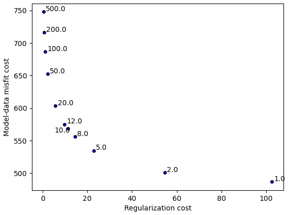
Figure 1 An L curve showing the trade-off between model misfit (first and second terms of Eq. 32) and the regularization cost (the second terms of Eq. 32 divided by γ). Associated values of the regularization parameter γ are shown. In all optimizations, δ is equal to 10⁻⁵, and observational points occur at intervals of 2 km.

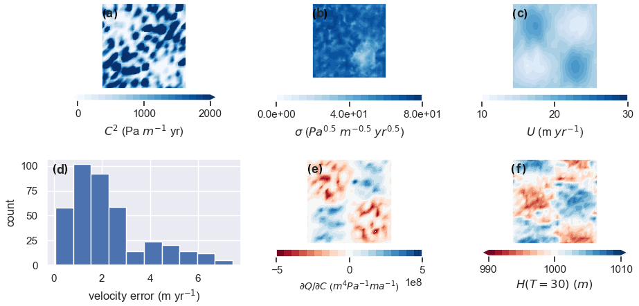
While misfit does not vary greatly in a proportional sense, it suggests γ=10 as a reasonable trade-off between misfit and regularization. Figure 2 displays results of an inversion with a “strong” level of regularization (γ=50; referred to below as the γ₅₀ experiment). The resulting C is relatively smooth (Fig. 2a), and the misfit is generally small though with some outliers (Fig. 2d). (Misfit is displayed as a histogram of errors – obtained by interpolating the finite-element solution to the sampled velocity locations – rather than as a spatially continuous function to emphasize the discrete nature of the model–data misfit.) Figure 3 gives equivalent results for a “weak” regularization inversion (γ=1; referred to below as the γ₁ experiment). The misfit distribution is similar, but the inverted sliding parameter is significantly noisier as a result of weaker constraints on these “noisy” modes by the prior.

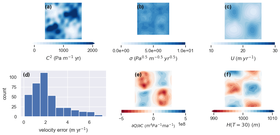
Figure 2 Results of the control method inversion with γ=50. (a) The recovered basal traction C². (b) The pointwise standard deviation of the sliding parameter C. (c) The surface speed associated with the inverted C. (d) Histogram of model–data velocity misfit (where misfit is the 2-norm of the difference of observed and modeled velocity). (e) The sensitivity of $Q_{\mathrm{30}}^{\mathrm{IS}}$ to the sliding parameter. (f) Thickness after 30 years of time stepping.

Figure 3 Similar to Fig. 2 but with γ=1. Note the difference in color map with Fig. 2b.

The effect of regularization on reduction of uncertainty can be seen from examining the eigenvalues defined by Eq. (14). More precisely, the ratio $\mathrm{1}/(\mathrm{1}+{\mathit{\lambda }}_i)$, where λ_i is the ith leading eigenvalue, is examined. As shown in Sect. 2.4, this ratio gives the reduction in variance of the associated eigenvector in the posterior PDF relative to the prior distribution. In Fig. 4a this quantity is shown for the eigenvalue spectra corresponding to γ=1, 10, and 50. For all inversions, uncertainty reduction is several orders of magnitude for the leading eigenvalues, but the tails of the spectra are quite different. In the case of strong regularization, there is little reduction in variance beyond i∼ 100, while in the weakly regularized case there is considerable reduction across the entire spectrum. This discrepancy can be interpreted as the prior providing so little information in the low-regularization case that the information provided by the inversion reduces uncertainty across all modes. The comparison of eigenvalue spectra across experiments is only meaningful to the extent that the corresponding eigenvectors are equivalent. A comparison between the four leading eigenvectors in the high- and low-regularization experiments (Fig. 5) shows they are not equivalent but have the same overall structure. (Differences arise due to ${\stackrel{\mathrm{‾}}{c}}_{\mathrm{MAP}}$ but also due to differences in Γ_prior.)

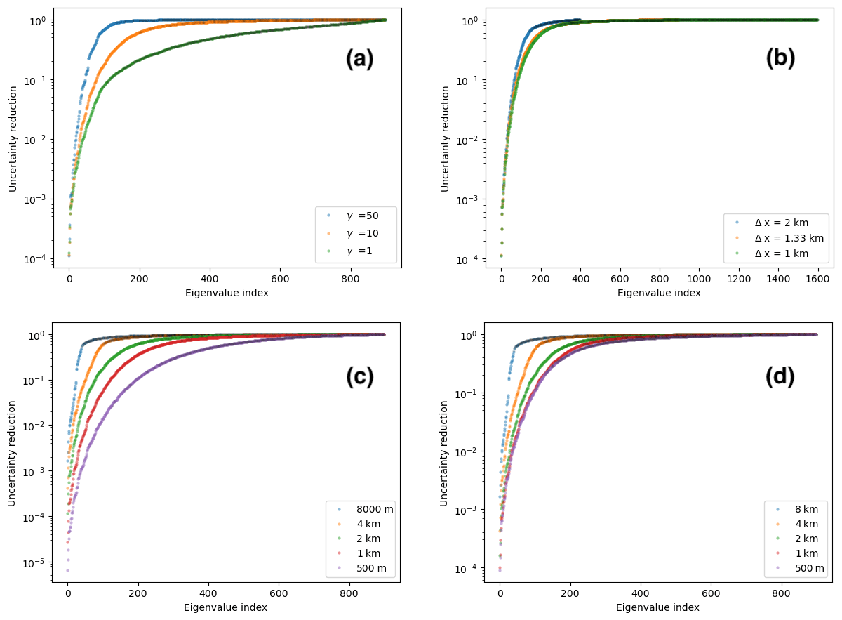
Figure 4 Uncertainty reduction factor $\mathrm{1}/(\mathrm{1}+{\mathit{\lambda }}_k)$ versus eigenvalue index k for a range of experiments. (a) Dependence of reduction spectra on the regularization parameter γ_α. (b) Dependence of reduction spectra on model resolution. (c) Dependence of reduction spectra on the density of observational sample points. (d) Dependence of reduction spectra on the density of observational sample points with nonzero observational covariance.

Approximating the posterior covariance of $\stackrel{\mathrm{‾}}{c}$, Γ_post, also allows an estimation of Σ_C, the pointwise variance of C. This is done via calculation of the square root of the diagonal entries of Γ_post, i.e., the standard deviation of the marginal distributions of the coefficients of $\stackrel{\mathrm{‾}}{c}$. Σ_C is shown for the inversions discussed above in Figs. 2b and 3b. Pointwise uncertainties in γ₁ are 5–10 times larger than in γ₅₀. For γ₅₀ there is a clear pattern of higher uncertainty where the bed is weaker (i.e., C is smaller), though for γ₁ it is difficult to discern any pattern.

5.1.2 Effect of resolution

The impacts of grid resolution on eigenvalue spectra are investigated (Fig. 4b). In Isaac et al. (2015), it was shown that the leading eigenvalues were independent of the numerical mesh, implying that the leading eigenvectors – the patterns for which uncertainties are quantified – are not dependent on the dimension of the parameter space (which would be an undesirable property). Our spectra suggest that at 2 km resolution, there is mesh dependence, but the spectra for 1.33 and 1 km resolution are in close agreement, suggesting mesh independence (Isaac et al., 2015). Consistent values of γ and δ are used for these experiments, meaning the results of the L curve in Fig. 1 are not dependent on model resolution.

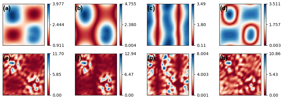
Figure 5 (a–d) Leading four eigenvectors of C in the γ₅₀ experiment. (e–g) Leading four eigenvectors of C in the γ₁ experiment.

5.2 Propagation of uncertainties

5.3 Linear propagation of uncertainties

The low-rank approximation of the posterior covariance of $\stackrel{\mathrm{‾}}{c}$ found with Eq. (20) can be used to estimate the uncertainty of $Q_T^{\mathrm{IS}}$ using Eq. (22). To do so, $\frac{\partial Q_T^{\mathrm{IS}}}{\partial \stackrel{\mathrm{‾}}{c}}$ must be found, which is done using algorithmic differentiation of the time-dependent model as described in Sect. 4. Figures 2e and 3e show $\frac{\partial Q_{\mathrm{30}}^{\mathrm{IS}}}{\partial \stackrel{\mathrm{‾}}{c}}$ arising from their respective inversions. There is small-scale noise in the low-regularization experiment (γ₁), but the general pattern and magnitude between the two gradients are similar, with strengthening of weak-bedded areas and weakening of strong-bedded areas both leading to an increase in the fourth-order moment of thickness. The gradient of $Q_T^{\mathrm{IS}}$ with respect to $\stackrel{\mathrm{‾}}{c}$ is found for intermediate values of T over the 30-year interval, with $\mathit{\sigma }\left(Q_T^{\mathrm{IS}}\right)$ calculated at these times – which can then be linearly interpolated to find a trajectory of uncertainty. In our experiments we find the gradient of $Q_T^{\mathrm{IS}}$ every 6 years. In Fig. 6a these trajectories are shown for the γ₅₀ and γ₁ experiments, plotted as a 1σ error interval around the calculated trajectory of $Q_T^{\mathrm{IS}}$.

Figure 6 (a) Paths of $Q_T^{\mathrm{IS}}$ in the γ₅₀ experiment (blue) and γ₁ experiment (green). Shading shows the 1σ uncertainty interval for each trajectory calculated by projecting the Hessian-based (posterior) uncertainty along the linearized trajectory. (b) Uncertainties in the time-dependent experiments over time. Dashed lines: prior uncertainties projected along the linearized $Q_T^{\mathrm{IS}}$ trajectory. Solid lines: Hessian-based posterior uncertainties projected along the linearized trajectory. Markers: standard deviation of $Q_T^{\mathrm{IS}}$ from sampling the posterior density. In both panels, green corresponds to γ₅₀ and blue to γ₁.

The trajectory of uncertainties for γ₅₀ and γ₁ can also be seen in Fig. 6b compared against the trajectories of

$$\begin{array}{}\text{(34)}& \left(\right({\displaystyle \frac{\partial Q_T^{\mathrm{IS}}}{\partial \stackrel{\mathrm{‾}}{c}}}{)}^T{\mathbf{\Gamma }}_{\mathrm{prior}}\left({\displaystyle \frac{\partial Q_T^{\mathrm{IS}}}{\partial \stackrel{\mathrm{‾}}{c}}}\right){)}^{\mathrm{1}/\mathrm{2}},\end{array}$$

i.e., the prior uncertainty linearly projected along the trajectory of $Q_T^{\mathrm{IS}}$. This uncertainty measure is not physically meaningful as it depends on the calculated $\partial Q_T^{\mathrm{IS}}/\partial \stackrel{\mathrm{‾}}{c}$, which in turn depends on the inversion for $\stackrel{\mathrm{‾}}{c}$ and the related trajectory of $Q_T^{\mathrm{IS}}$ – and a random sample from the prior distribution of $\stackrel{\mathrm{‾}}{c}$ is unlikely to yield such a trajectory. Still, it serves as a measure of decrease in uncertainty arising from the information encapsulated in the observations and model physics.

$Q_T^{\mathrm{IS}}$ is greater in magnitude in the γ=1 experiment than in the γ=50 experiment at all times – and it can be seen from the uncertainty of the γ₁ trajectory that this difference is statistically significant. The two experiments have differing (inverse) solutions, with the γ₁ inversion favoring a closer fit to noisy observations at the cost of small-scale variability in the inverse solution. Our quantity of interest (the fourth-order moment of thickness) is sensitive to this small-scale variability, so uniformity of trajectories of $Q_T^{\mathrm{IS}}$ would not be expected. At the same time, the level of QoI uncertainty in the γ₁ trajectory relative to that of the γ₅₀ QoI uncertainty is much smaller than the relative magnitudes of the inversion uncertainties (see Figs. 2b, 3b) would suggest. This can be rationalized by considering Eq. (22): uncertainty in the QoI will depend on the extent to which uncertain parameter modes project onto the gradient of the QoI with respect to the parameters. While the γ₁ inversion results are overall more uncertain, the leading order modes are still constrained quite strongly. Thus, while $Q_T^{\mathrm{IS}}$ is to a degree sensitive to small-scale variability it may still filter the most uncertain modes of the γ₁ inversion, resulting in a smaller QoI uncertainty than expected. In fact, it can be seen from Fig. 6b that despite the large differences in prior distributions between γ₅₀ and γ₁, the projections of the respective prior covariances along the trajectory of $Q_T^{\mathrm{IS}}$ are very similar, suggesting that the gradient of $Q_T^{\mathrm{IS}}$ does not project strongly on the modes which are poorly constrained in the γ₁ experiment.

5.3.1 Direct sampling of QoI uncertainties

Ideally, the assumptions implicit in the calculation of QoI uncertainties shown in Fig. 6a would be tested through unbiased sampling from the prior distributions of $\stackrel{\mathrm{‾}}{c}$, followed by using the sampled parameters to initialize the time-dependent model and generating a sample of trajectories of $Q_T^{\mathrm{IS}}$ and finally scaling the probability of each member of the ensemble based on the observational likelihood function $p\left({\stackrel{\mathrm{˘}}{\mathit{u}}}_{\mathrm{obs}}\right|\stackrel{\mathrm{‾}}{c})$. However, given the dimension of the space containing $\stackrel{\mathrm{‾}}{c}$ (equal to 900 in our idealized experiment but on the order of 10⁴–10⁵ in more realistic experiments), the number of samples required to ensure non-negligible likelihoods would not be tractable without a sophisticated sampling strategy such as Markov chain Monte Carlo (MCMC) methods (Tierney, 1994) (and even then it may require approximations similar to those described above; Martin et al., 2012; Petra et al., 2014). However, such approaches are beyond the scope of this study.

The assumptions in our propagation of observational and prior uncertainty to the quantity of interest uncertainty are (i) Gaussianity of the distribution of $\stackrel{\mathrm{‾}}{c}$ and (ii) linearity of the map from $\stackrel{\mathrm{‾}}{c}$ to QoI. While (i) cannot be tested for the reasons stated above, (ii) can be tested by sampling from the calculated posterior distribution of $\stackrel{\mathrm{‾}}{c}$, initializing the time-dependent model, and finding the ensemble variance and standard deviation of $Q_T^{\mathrm{IS}}$. Our strategy for sampling from the posterior is described below and is based on the derivation in Bui-Thanh et al. (2013).

A randomly sampled vector $\stackrel{\mathrm{‾}}{x}$ will have covariance Γ_post and mean ${\stackrel{\mathrm{‾}}{c}}_{\mathrm{MAP}}$ if it is generated via

$$\begin{array}{}\text{(35)}& \stackrel{\mathrm{‾}}{x}={\stackrel{\mathrm{‾}}{c}}_{\mathrm{MAP}}+\mathbf{K}\stackrel{\mathrm{‾}}{N},\end{array}$$

where $\stackrel{\mathrm{‾}}{N}$ is a sample from a multivariate normal distribution $\mathbb{N}\sim \mathcal{N}(\mathrm{0},\mathbf{I})$ of the same dimension as $\stackrel{\mathrm{‾}}{c}$, and K is such that KK^T=Γ_post. Hence, it is required to find a suitable K. We restate the generalized eigenvalue problem ${\mathbf{H}}_{\mathrm{mis}}\mathbf{C}={\mathrm{\Gamma }}_{\mathrm{prior}}^{-\mathrm{1}}\mathbf{C}\mathbf{\Lambda }$. Since C is orthogonal in the inverse prior covariance (see Eq. 16), the identity matrix I can be spectrally decomposed in ${\stackrel{\mathrm{‾}}{c}}_i$ (the columns of C):

$$\begin{array}{}\text{(36)}& ({\displaystyle }\sum {\stackrel{\mathrm{‾}}{c}}_i{\stackrel{\mathrm{‾}}{c}}_i^T{\mathbf{\Gamma }}_{\mathrm{prior}}^{-\mathrm{1}})=\mathbf{I}.\end{array}$$

Rearranging gives $\sum {\stackrel{\mathrm{‾}}{c}}_i{\stackrel{\mathrm{‾}}{c}}_i^T={\mathbf{\Gamma }}_{\mathrm{prior}}$, so (see Eq. 20)

$$\begin{array}{ll}{\displaystyle }{\mathbf{\Gamma }}_{\mathrm{post}}& {\displaystyle }\sim {\mathbf{\Gamma }}_{\mathrm{prior}}-{\mathbf{C}}_r{\mathbf{D}}_r{\mathbf{C}}_r^T\\ {\displaystyle }& {\displaystyle }={\displaystyle }\sum _{i=\mathrm{1}}^n{\stackrel{\mathrm{‾}}{c}}_i{\stackrel{\mathrm{‾}}{c}}_i^T-{\displaystyle }\sum _{i=\mathrm{1}}^r{\stackrel{\mathrm{‾}}{c}}_i{\stackrel{\mathrm{‾}}{c}}_i^T\left({\displaystyle \frac{{\mathit{\lambda }}_i}{\mathrm{1}+{\mathit{\lambda }}_i}}\right)\\ \text{(37)}& {\displaystyle }& {\displaystyle }={\displaystyle }\sum _{i=r+\mathrm{1}}^n{\stackrel{\mathrm{‾}}{c}}_i{\stackrel{\mathrm{‾}}{c}}_i^T+{\displaystyle }\sum _{i=\mathrm{1}}^r{\stackrel{\mathrm{‾}}{c}}_i{\stackrel{\mathrm{‾}}{c}}_i^T\left({\displaystyle \frac{\mathrm{1}}{\mathrm{1}+{\mathit{\lambda }}_i}}\right).\end{array}$$

We define the matrix B:

$$\begin{array}{ll}{\displaystyle }\mathbf{B}& {\displaystyle }={\mathbf{\Gamma }}_{\mathrm{prior}}+{\displaystyle }\sum _{i=\mathrm{1}}^r{\stackrel{\mathrm{‾}}{c}}_i{\stackrel{\mathrm{‾}}{c}}_i^T({\displaystyle \frac{{\mathit{\lambda }}_i}{\sqrt{\mathrm{1}+{\mathit{\lambda }}_i}}}-\mathrm{1})\\ \text{(38)}& {\displaystyle }& {\displaystyle }={\displaystyle }\sum _{i=r+\mathrm{1}}^n{\stackrel{\mathrm{‾}}{c}}_i{\stackrel{\mathrm{‾}}{c}}_i^T+{\displaystyle }\sum _{i=\mathrm{1}}^r{\stackrel{\mathrm{‾}}{c}}_i{\stackrel{\mathrm{‾}}{c}}_i^T\left({\displaystyle \frac{\mathrm{1}}{\sqrt{\mathrm{1}+{\mathit{\lambda }}_i}}}\right).\end{array}$$

And due to the ${\mathbf{\Gamma }}_{\mathrm{prior}}^{-\mathrm{1}}$ orthogonality of C,

$$\begin{array}{ll}{\displaystyle }\mathbf{B}{\mathbf{\Gamma }}_{\mathrm{prior}}^{-\mathrm{1}}{\mathbf{B}}^T& {\displaystyle }={\displaystyle }\sum _{i=r+\mathrm{1}}^n{\stackrel{\mathrm{‾}}{c}}_i{\stackrel{\mathrm{‾}}{c}}_i^T+{\displaystyle }\sum _{i=\mathrm{1}}^r{\stackrel{\mathrm{‾}}{c}}_i{\stackrel{\mathrm{‾}}{c}}_i^T\left({\displaystyle \frac{\mathrm{1}}{\mathrm{1}+{\mathit{\lambda }}_i}}\right)\\ \text{(39)}& {\displaystyle }& {\displaystyle }={\mathbf{\Gamma }}_{\mathrm{post}}.\end{array}$$

Therefore, a suitable K is given by (see Eq. 11)

$$\begin{array}{}\text{(40)}& \mathbf{B}{\mathbf{\Gamma }}_{\mathrm{prior}}^{-\mathrm{1}/\mathrm{2}}={\mathbf{BLM}}^{-\mathrm{1}/\mathrm{2}}.\end{array}$$

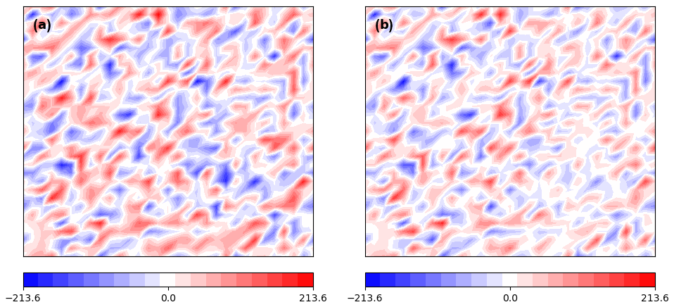
The action of the square root of the mass matrix M is found by a Taylor series approach (Higham, 2008, Eq. 6.38). Figure 7 shows a result of sampling from the posterior in the γ₅₀ experiment. To the left (panel a), a realization of the prior distribution, with mean zero and covariance Γ_prior, is displayed. (This realization is found similarly to that of the posterior, with the formula $\stackrel{\mathrm{‾}}{N}{\mathbf{\Gamma }}_{\mathrm{prior}}^{\mathrm{1}/\mathrm{2}}$.) To the right (panel b), a realization of the posterior distribution is shown with the mean ${\stackrel{\mathrm{‾}}{c}}_{\mathrm{MAP}}$ removed. (Note that both samples are derived from the same realization of ℕ.) From comparing the images it can be seen that variance is greatly reduced, particularly at medium to large scales. By contrast, when the posterior distribution of γ₁ is sampled, the result is very similar to the prior. Very little reduction of variance is visually apparent, especially at small scales.

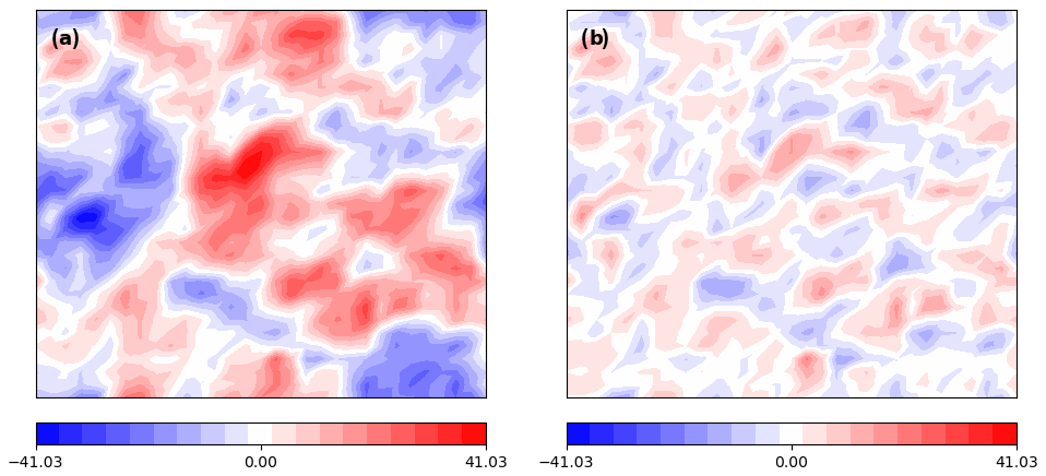
Figure 7 (a) A realization of the prior density of C for the γ₅₀ experiment. (b) A realization of the posterior density of C for the γ₅₀ experiment with mean ${\stackrel{\mathrm{‾}}{c}}_{\mathrm{MAP}}$ removed.

Using this method of sampling the posterior, an ensemble of 1000 30-year runs is carried out for both low- and high-regularization experiments (γ₁ and γ₅₀, respectively), and standard deviations of $Q_T^{\mathrm{IS}}$ are calculated at discrete times. Values are plotted in Fig. 6b. (For each such calculation, the variance quickly converged to the value shown, so it is unlikely that the quantity of interest is under-sampled.) In the γ₅₀ experiment there is strong agreement between the sampled uncertainties and those found via projecting C uncertainty along the linearized QoI trajectory, suggesting that the linear approximation inherent in Eq. (22) is appropriate. In contrast, there are large discrepancies in the γ₁ case. It is likely that the small-scale noise inherent in the low-regularization samples (see Fig. 8) impacts the quantity of interest strongly enough that the linear approximation in Eq. (22) breaks down – despite the fact that this noise does not strongly affect the cost function J^c. As mentioned in Sect. 5.2, this may be due to the nature of the QoI. In the γ₁₀ experiment (not shown), the disagreement in uncertainties is on the order of 30 – greater than for the γ₅₀ experiment but far less than for γ₁.

Figure 8 (a) A realization of the prior density of C for the γ₁ experiment. (b) A realization of the posterior density of C for the γ₁ experiment with mean ${\stackrel{\mathrm{‾}}{c}}_{\mathrm{MAP}}$ removed. Note the difference in color map with Fig. 7.

5.4 Observational density and uncertainty

In all results presented to this point, the imposed locations for observational data ${\stackrel{\mathrm{˘}}{u}}_{\mathrm{obs}}$ and ${\stackrel{\mathrm{˘}}{v}}_{\mathrm{obs}}$ lie on a regular grid with a spacing of 2 km. Here we consider the effects of the observational spatial density on the reduction of uncertainty in $\stackrel{\mathrm{‾}}{c}$.

5.4.1 Effect of observation spacing

Eigendecompositions of the prior-preconditioned misfit Hessian (${\widehat{\mathbf{H}}}_{\mathrm{mis}}$) are carried out for observational spacings of 500 m, 1 km, 2 km, 4 km, and 8 km. (The 2 km case corresponds to the γ₁₀ experiment in Fig. 4a.) In all other respects the experiments are identical. Results are shown for comparison in Fig. 4c. Increasing spatial density appears to reduce uncertainty: in the 500 m case, there is considerable uncertainty reduction even in cases in which there is almost no reduction in coarser-observation cases. The result is intuitive: each increase in observational density quadruples the number of independent constraints, effectively adding more information (though a more sophisticated framework is required to quantify the information increase from a given observation; e.g., Alexanderian et al., 2014).

Comparison of eigenspectra relies on the corresponding eigenvectors being the same, or similar, between the experiments. As in the regularization and resolution experiments, the eigenvectors depend on the exact form of ${\widehat{\mathbf{H}}}_{\mathrm{mis}}$, which in turn depends on ${\stackrel{\mathrm{‾}}{c}}_{\mathrm{MAP}}$; this may differ between the experiments due to the differing number of points. However, they are likely to be of similar patterns (on the basis of the results of Sect. 5.1.1).

5.4.2 Effect of observational covariance

The results described above imply that posterior uncertainty could be made arbitrarily small by increasing the spatial density of observations (although we do not examine observations more dense than 500 m). However, the decreasing uncertainty relies on the observations being statistically independent, which is unlikely to be the case as observations become more and more dense. We consider here the implications of a nonzero spatial covariance. Rather than imposing a realistic observational covariance matrix, we consider a simplified covariance structure in which correlations decay isotropically. That is, our observational covariance matrix Γ_u,obs is given by

$$\begin{array}{}\text{(41)}& {\mathbf{\Gamma }}_{\mathrm{u},\mathrm{obs}}(i,j)={\mathit{\sigma }}_{\mathrm{u},\mathrm{obs}}^{\mathrm{2}}{e}^{-\frac{|{\mathit{x}}_i-{\mathit{x}}_j{|}^{\mathrm{2}}}{d_{\mathrm{auto}}^{\mathrm{2}}}}.\end{array}$$

Here, σ_u,obs is the observational uncertainty and x_i is the position of observation i. (By contrast, Γ_u,obs in all experiments described above is a diagonal matrix with entries ${\mathit{\sigma }}_{\mathrm{u},\mathrm{obs}}^{\mathrm{2}}$.) A value of 1 m per year is used for σ_u,obs, as in all previous experiments, and d_auto is set to 750 m. We assert that the observations of orthogonal velocity components are independent; i.e., Γ_u,obs is block-diagonal with each block corresponding to a velocity component. While velocity component uncertainties are likely to correlate, introducing spatial correlation among the individual components already greatly changes the effect of observation spacing on uncertainty reduction, as seen in Fig. 4d. When observational spacing is large compared to d_auto, an increase in density has a similar effect as that seen in the zero-spatial-correlation case (Fig. 4c). But for observational spacing on the order of d_auto, additional observations have a minimal effect.

6 Gauss–Newton approximation to the Hessian

Section 2.2 introduces the Hessian of the cost function and gives an expression for the posterior covariance when the parameter-to-observable map $\stackrel{\mathrm{˘}}{f}$ is linear (Eq. 5). The first term in brackets on the right-hand side of Eq. (5), which we write here as

$$\begin{array}{}\text{(42)}& \left({\displaystyle \frac{\partial \stackrel{\mathrm{˘}}{f}}{\partial \stackrel{\mathrm{‾}}{c}}}{)}^T{\mathbf{\Gamma }}_{\mathrm{obs}}^{-\mathrm{1}}\right({\displaystyle \frac{\partial \stackrel{\mathrm{˘}}{f}}{\partial \stackrel{\mathrm{‾}}{c}}}),\end{array}$$

is the Hessian of the misfit cost function $J_{\mathrm{mis}}^{\mathrm{c}}$ under the condition that $\stackrel{\mathrm{˘}}{f}$ is linear. It is quite often used as an approximation to the Hessian for the purpose of covariance estimates even when $\stackrel{\mathrm{˘}}{f}$ is nonlinear (Kaminski et al., 2015; Loose et al., 2020) and is referred to as the Gauss–Newton approximation to the Hessian (GNaH). The GNaH has the advantage of avoiding the complexity of finding second-order derivatives. It also has the property that the misfit Hessian (or rather, its approximation) is positive semidefinite – this is not necessarily true of the “full” Hessian even when the cost function J^c is minimized, meaning the eigendecomposition described in Sect. 2.4 can have negative eigenvalues.

In the context of our idealized experiments we calculate the GNaH (or rather, its action on a vector) to compare against the full Hessian. The tlm_adjoint library's functionality is employed as follows. For a given finite-element coefficient vector $\stackrel{\mathrm{‾}}{\mathit{\xi }}$, the GNaH action can be written as

$$\begin{array}{}\text{(43)}& \left({\displaystyle \frac{\partial \stackrel{\mathrm{˘}}{f}}{\partial \stackrel{\mathrm{‾}}{c}}}{)}^T{\mathbf{\Gamma }}_{\mathrm{obs}}^{-\mathrm{1}}\right({\displaystyle \frac{\partial \stackrel{\mathrm{˘}}{f}}{\partial \stackrel{\mathrm{‾}}{c}}})\stackrel{\mathrm{‾}}{\mathit{\xi }}=({\displaystyle \frac{\partial \stackrel{\mathrm{˘}}{f}}{\partial \stackrel{\mathrm{‾}}{c}}}{)}^T\stackrel{\mathrm{˘}}{\mathit{\eta }},\end{array}$$

where $\stackrel{\mathrm{˘}}{\mathit{\eta }}$ is obtained through the action of the tangent linear model $(\partial \stackrel{\mathrm{˘}}{f}/\partial \stackrel{\mathrm{‾}}{c})$ on $\stackrel{\mathrm{‾}}{\mathit{\xi }}$ and the action of the inverse observational covariance on the result. The GNaH action is then obtained through the action of the adjoint of the Jacobian of the parameter-to-observable map, $(\partial \stackrel{\mathrm{˘}}{f}/\partial \stackrel{\mathrm{‾}}{c}{)}^T$.

In Fig. 9 we examine the effects of using the GNaH rather than the Hessian in our Hessian-based UQ framework. This is done for just a single experiment with 1.33 km elements, 2 km observational spacing, and regularization with γ=10. Examining the uncertainty reduction (Fig. 9a), the first ∼ 80 eigenvalues are nearly identical, but after this the uncertainty reduction approaches 1 much faster (or, equivalently, the eigenvalues decay much faster) with the GNaH. In terms of posterior QoI uncertainty (Fig. 9b), $\mathit{\sigma }\left(Q_T^{\mathrm{IS}}\right)$ is slightly smaller with the GNaH, but the difference is very small and only visible at later times.

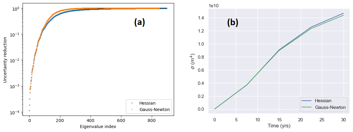
Figure 9 (a) Uncertainty reduction factor $\mathrm{1}/(\mathrm{1}+{\mathit{\lambda }}_k)$ versus eigenvalue index k for γ=10 and observational spacing of 2 km, found with the full Hessian and Gauss–Newton approximation. (b) Hessian-based posterior uncertainties of $Q_T^{\mathrm{IS}}$ over time based on the full Hessian and Gauss–Newton approximations.

7 Discussion and conclusions

The inversion of surface velocities for basal conditions is ubiquitous in ice sheet modeling – but in most studies in which this is done, the uncertainty of the resulting parameter fields is not considered, and the implications of this parametric uncertainty for projection uncertainty are not quantified. We introduce fenics_ice, a numerical Python code which solves the shallow shelf approximation (SSA) for ice sheet dynamics. The code uses the FEniCS library to facilitate a finite-element solution of partial differential equations. Algorithmic differentiation is implemented with the tlm_adjoint library, allowing for adjoint generation of the time-dependent and time-independent versions of the SSA. This feature is used to aid inversions of surface velocity for parameter fields such as the basal sliding parameter. In addition, the tlm_adjoint library allows efficient second-order differentiation of the inversion cost function, allowing a low-rank approximation to the cost function Hessian. We utilize this ability to exploit the connection between the control method inversions typically carried out with ice sheet models and a Bayesian characterization of the uncertainty of the inverted parameter field. This interpretation allows us to form a local approximation to the posterior probability density at the maximum a posteriori (MAP) point. With a time-dependent quantity of interest (QoI) which depends on the outcome of the inversion, the adjoint features of fenics_ice allow linear propagation of parametric uncertainty to QoI uncertainty.

We apply our framework to a simple idealized test case, Experiment C of the ISMIP-HOM intercomparison protocol, involving an ice stream sliding across a doubly periodic domain with a varying basal friction parameter. An idealized time-varying QoI is defined, equivalent to the fourth moment of thickness in the domain, as thickness evolves due to mass continuity. The posterior probability density is examined, suggesting mesh independence (provided resolution is high enough). It is shown that the level of uncertainty reduction relative to the prior distribution depends on the amount of information in the prior (or, equivalently, the degree of regularization). Uncertainty of the QoI is found along its trajectory and is found to increase with time and also found to be larger with less-constrained priors. However, the difference in the uncertainty of the QoI is far less than that of the parametric uncertainty due to insensitivity of the QoI to high-frequency modes.

Sampling from our posterior allows us to test the linearity of the parameter-to-QoI mapping, and this approximation is seen to be accurate with a moderately strong prior. However, even with the relatively modest problem sizes considered, testing the validity of our local Gaussian approximation of the posterior probability density would require sophisticated sampling methods which are beyond the scope of our study. It is worth noting, though, that one such method, stochastic Newton MCMC (Martin et al., 2012; Petra et al., 2014), relies on the framework developed in this study (i.e., characterizing the local behavior of the posterior density through a Hessian-based approximation). Therefore, it may be a viable approach for non-Gaussian uncertainty quantification in future iterations.

The sensitivity of QoIs to small-scale variability is significant because not all glaciologically motivated QoIs are expected to have such sensitivities. For instance, the QoI considered by Isaac et al. (2015) was a contour integral of volume flux over the boundary of the domain, equivalent to a rate of change in ice volume – and such a quantity might be less sensitive to velocity gradients and small-scale thickness change in the domain interior. On the other hand, a forecast focused on the impact of evolving surface elevation on proliferation of surface lakes or on surface fractures might be very sensitive to such variability. Therefore, when considering parametric uncertainty, it should also be considered whether the nature of this uncertainty impacts the uncertainty of the intended quantity of interest.

A key difference between our approach and the control method inversions typically undertaken is the Euclidean inner product that appears in the misfit component of the cost function as opposed to an area integral of velocity misfit. As discussed in Sect. 2.3, the latter formulation leads to difficulties with a Bayesian interpretation by conflating the observational error covariance with mesh-dependent factors. In our study observation locations are imposed on a regular grid. It is shown that, with statistically independent observations, posterior uncertainty is continually reduced as the observational grid becomes more dense. When a spatial correlation of observations is considered, however, there is little reduction of uncertainty when adding observations beyond a certain spatial density. This result is of significance to ice sheet modeling: most ice sheet model studies which calibrate parameters to velocity observations (including those mentioned in the Introduction) do not consider the spatial correlation of observations. As discussed in Sect. 2.3, these studies express the model–data misfit as an area integral – meaning that, effectively, observations in adjacent model grid cells are considered independent. If grid cells are sufficiently large, this is likely a suitable approximation – though with higher and higher resolutions being used in ice sheet modeling studies (Cornford et al., 2013), it should be considered whether the spatial covariance of observations is such that it might affect results. Assessing such effects poses an additional challenge, however, as ice sheet velocity products are not generally released with spatial error covariance information (Rignot et al., 2017).

Our study does not consider “joint” inversions, i.e., inversions with two or more parameter fields. With such inversions, complications can arise when both parameters affect the same observable, potentially leading to equifinality and/or ill-posedness. An example of such a pair is C, the sliding coefficient, and B, the ice stiffness in the nonlinear Glen's rheology (see Eq. 24), which can both strongly affect ice speeds in a range of settings. The version of fenics_ice presented in this study is not capable of joint inversions or of Hessian vector products with multiple parameter fields; however, the technical hurdles to implementation are minor. More importantly, though, Hessian-based Bayesian uncertainty quantification with multiple parameter fields has not, to our knowledge, been carried out in an ice sheet modeling context and may present difficulties due to a larger problem space or the equifinality issues mentioned above. (Instead of performing a joint inversion, Babaniyi et al., 2021, use a Bayesian approximation error framework, treating the stiffness parameter as a random variable.) Nonetheless, the investigation of joint inversions and uncertainty quantification is a future research aim for fenics_ice.

Model uncertainty is not accounted for in our characterization of parametric uncertainty. In the expression for the posterior probability density (Eq. 4), the model misfit term is expressed as the difference between observed and modeled velocity, and the uncertainty is assumed to arise from the observation platform. In fact, the discrepancy between modeled and observed velocity is the sum of observation error, ϵ_obs, and model error, ϵ_model. This second error source can be considered a random variable, as it arises from incomplete knowledge about the ice sheet basal environment and material properties of the ice, as well as the approximations inherent in the shallow shelf approximation. Characterizing this uncertainty is challenging as it requires both perfect knowledge of the basal sliding parameter and observations with negligible error, and it is beyond the scope of our study. Future research, however, could involve using a model which implements the full Stokes solution (e.g., Gagliardini et al., 2010) to partially characterize this uncertainty or could make use of a multi-fidelity approach (Khodabakhshi et al., 2021).

A number of Hessian-based uncertainty quantification studies use the Gauss–Newton approximation to the Hessian (see Sect. 6), avoiding computation of higher-order derivatives of the model, but few studies have investigated the impact of neglecting these higher-order terms. For our idealized experiment we have compared uncertainty reduction and QoI uncertainty with both Gauss–Newton and full Hessian computation. There is negligible difference in terms of QoI uncertainty, but it remains to be seen if this is the case for more realistic experiments.

Our study does not consider time-dependent inversions, i.e., control methods wherein the cost function is time-dependent. While the majority of cost function inversions are time-independent, there are a growing number of studies carried out with time-dependent inversions (Larour et al., 2014; Goldberg et al., 2015), and it is possible that such methods may provide lower uncertainty in calibration of hidden parameters (simply by providing additional constraints) and hence in ice sheet projections. The fenics_ice (or rather tlm_adjoint) code is capable of eigendecomposition of Hessian matrices of time-dependent cost functions (Maddison et al., 2019), but time-dependent Hessian vector products are computationally expensive, requiring checkpointing and recomputation of both forward- and reverse-mode model information, and it is unlikely that full eigenvalue spectra can be found for even modestly sized problems. It is hopeful that for realistic problems of interest only a small fraction of eigenvalues will need to be found to accurately approximate the posterior covariance. Alternatively, the Gauss–Newton approximate Hessian might diminish some of the cost. Certainly more work is required in this area.