Nemo-Nordic 2.0: operational marine forecast model for the Baltic Sea

This paper describes Nemo-Nordic 2.0, an operational marine model for the Baltic Sea. The model is used for both near-real-time forecasts and hindcast purposes. It provides estimates of sea surface height, water temperature, salinity, and velocity, as well as sea ice concentration and thickness. The model is based on the NEMO (Nucleus for European Modelling of the Ocean) circulation model and the previous Nemo-Nordic 1.0 configuration by Hordoir et al. (2019). The most notable updates include the switch from NEMO version 3.6 to 4.0, updated model bathymetry, and revised bottom friction formulation. The model domain covers the Baltic Sea and the North Sea with approximately 1 nmi resolution. Vertical grid resolution has been increased from 3 to 1 m in the surface layer. In addition, the numerical solver configuration has been revised to reduce artificial mixing to improve the representation of inflow events. Sea ice is modeled with the SI3 model instead of LIM3. The model is validated against sea level, water temperature, and salinity observations, as well as Baltic Sea ice chart data for a 2-year hindcast simulation (October 2014 to September 2016). Sea level root mean square deviation (RMSD) is typically within 10 cm throughout the Baltic basin. Seasonal sea surface temperature variation is well captured, although the model exhibits a negative bias of approximately −0.5 ^∘C. Salinity RMSD is typically below 1.5 g kg⁻¹. The model captures the 2014 major Baltic inflow event and its propagation to the Gotland Deep. The model assessment demonstrates that Nemo-Nordic 2.0 can reproduce the hydrographic features of the Baltic Sea.

1 Introduction

The Baltic Sea is a brackish, semi-enclosed water body in northern Europe (Fig. 1). It has unique characteristics due to large freshwater input and restricted water exchange with the North Sea. Several ocean circulation models have been set up for the Baltic Sea with varying configurations (e.g., Lehmann, 1995; Meier et al., 1999; Funkquist and Kleine, 2007; Berg and Poulsen, 2012; Dietze et al., 2014; Gräwe et al., 2015a; Hordoir et al., 2019).

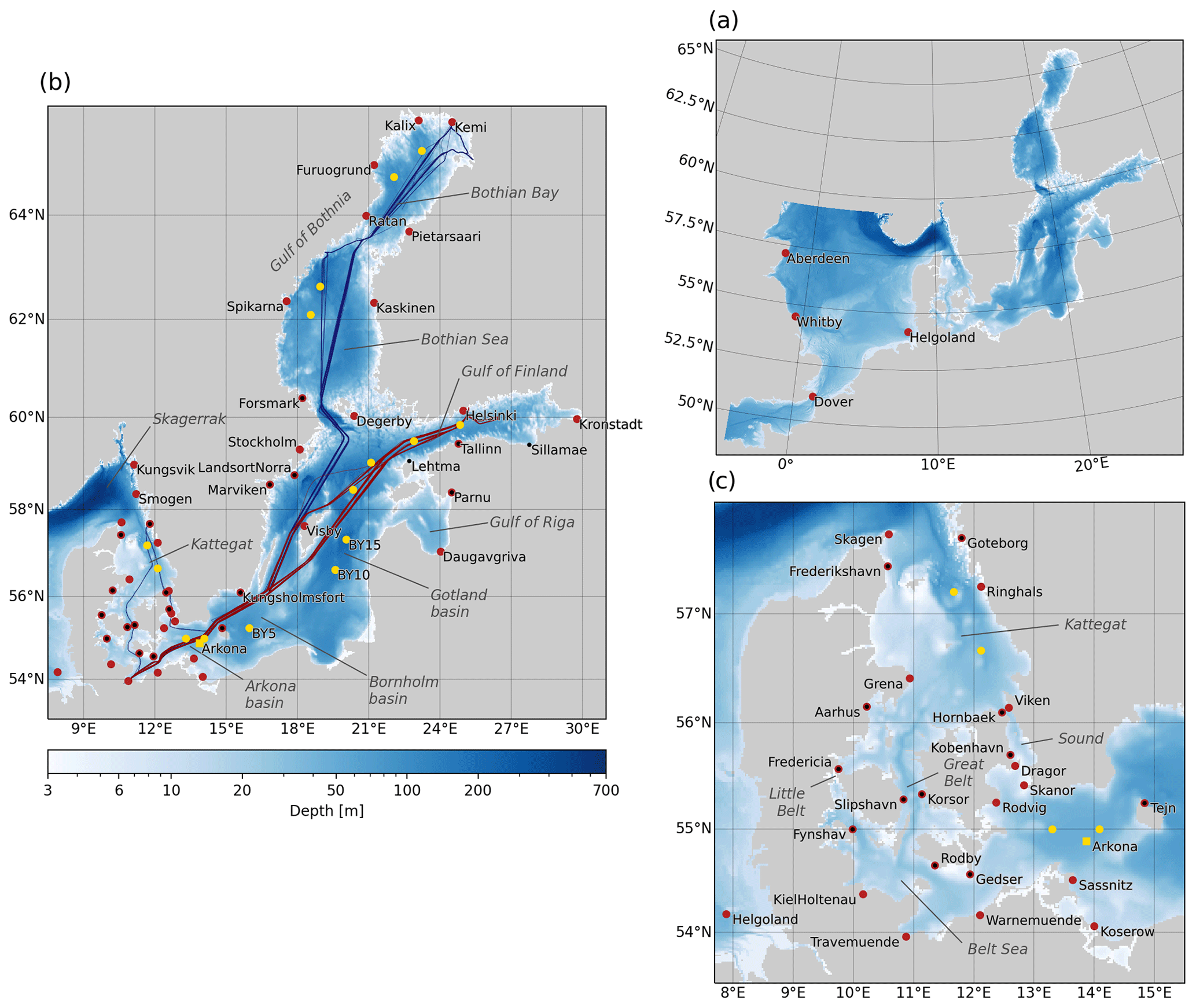
Figure 1 Computational domain and bathymetry; (a) the entire model domain, (b) the Baltic Sea, and the (c) Danish Straits region. Red and black dots indicate station locations with SSH and SST observations, respectively; yellow dots indicate vertical profile locations. Blue and red lines illustrate the TransPaper and FinnMaid ferry routes, respectively.

Operational ocean modeling has a fairly long history in the Baltic Sea, starting in the mid-1990s with HIROMB (High Resolution Operational Model for the Baltic). It was a cooperation involving many Baltic institutes that gathered around a common circulation model with the same name. The cooperation itself later became the modeling part of the Baltic Operational Oceanographic System (BOOS; https://boos.org, last access: 29 March 2021; She et al., 2020), or the BOOS Modelling Programme. The HIROMB model existed in several branches in different institutes for many years, e.g., the HIROMB model (Funkquist and Kleine, 2007; Axell, 2013) at the Swedish Meteorological and Hydrological Institute (SMHI) and the HIROMB BOOS Model (HBM; Berg and Poulsen, 2012). The first version of a common ocean circulation model built around the Nucleus for European Modelling of the Ocean (NEMO) was called Nemo-Nordic 1.0 and was described and validated by Pemberton et al. (2017) and Hordoir et al. (2019). It was based on NEMO version 3.6 and was coupled to the integrated ice model LIM3 (Vancoppenolle et al., 2009).

In this paper, we present an updated Nemo-Nordic 2.0 model for the Baltic Sea based on the NEMO circulation model version 4.0 (Madec et al., 2019). The model domain covers the North Sea and Baltic Sea (Fig. 1). The setup is based on the Nemo-Nordic 1.0 configuration (Hordoir et al., 2019). Compared to Nemo-Nordic 1.0, the most notable updates are the switch from NEMO 3.6 to NEMO 4.0, updated bathymetry, and revised bottom friction formulation. Vertical grid resolution has been increased in the surface layer from 3 to 1 m. We have also revised the numerical schemes (e.g., advection of momentum and tracers) to reduce artificial mixing. Finally, NEMO 4.0 uses the SI3 sea ice model instead of LIM3.

Modeling the circulation in the Baltic Sea is challenging due to the complex topography, strong stratification, and dense inflows related to major Baltic inflow (MBI) events (Mohrholz et al., 2015; Gräwe et al., 2015b; Mohrholz, 2018). Due to the complex nonlinear interaction with the North Sea (Gustafsson, 1997; Gustafsson and Andersson, 2001), it is widely accepted that the North Sea and Baltic Sea must be modeled as a single coupled system (Daewel and Schrum, 2013; Pätsch et al., 2017; Hordoir et al., 2019). Water exchange in the system is governed by the fluxes between the sub-basins. Many constraining regions, such as the Danish Straits and the Archipelago Sea, are characterized by fine-scale bathymetric features that are difficult to resolve in operational models. Representing the Danish Straits region, for example, requires sub-kilometer-scale horizontal resolution (She et al., 2007; Gräwe et al., 2015a; Stanev et al., 2018).

Salt pulses propagate as a density-driven bottom current from basin to basin. In circulation models, artificial numerical mixing can slow down or completely arrest the propagation of the current (Hofmeister et al., 2011; Klingbeil et al., 2014). Spurious vertical mixing can also cause excessive ventilation of the oxygen-depleted deep waters (Rennau and Burchard, 2009). In finite-volume models, the accuracy of the advection scheme has a significant impact on the level of numerical mixing (Zalesak, 1979; Hourdin and Armengaud, 1999; Lévy et al., 2001; Klingbeil et al., 2014). Previous studies suggest that vertical grid resolution plays an important role in retaining the salt pulse density structure in the Baltic Sea (Hofmeister et al., 2011; Gräwe et al., 2015a).

The aim of this article is to validate the Nemo-Nordic 2.0 model configuration. The configuration is used in the EU Copernicus Marine Service for both near-real-time forecasts and multiyear hindcast simulations for the Baltic Sea. The presented validation is based on a 2-year hindcast simulation that uses similar forcing as the operational configuration. The presented validation run uses a 3 km DMI HIRLAM atmospheric forcing, whereas the operational model will use 2.5 km MetCoOP HARMONIE model forecast padded with ECMWF HRES forecast data in North Sea regions outside the MetCoOP domain.

The model skill is assessed with respect to variables that are of interest to users: sea surface height (SSH), water temperature, and salinity, as well as sea ice coverage using observations. Observational data from tide gauges, FerryBox instruments, vertical profiles, and ice charts are used. The model configuration and observation data sets used are presented in Sect. 2. Section 3 presents the model assessment metrics, followed by a discussion and conclusions in Sect. 4.

2 Methods

2.1 Model domain and configuration

The presented model setup is an updated version of the Nemo-Nordic 1.0 configuration (Hordoir et al., 2019) implemented on NEMO version 4.0 (Madec et al., 2019; subversion repository revision 11281). Compared to Nemo-Nordic 1.0, the main improvements are the updated NEMO model version, switching from the LIM3 sea ice model to SI3, updated model bathymetry and land mask, revised bottom friction formulation, revised vertical grid, and revised solver options to reduce numerical mixing.

The grid covers the North Sea and Baltic Sea, spanning from 4.15278^∘ W to 30.18021^∘ E and 48.4917 to 65.8914216^∘ N (Fig. 1a). The horizontal grid resolution is 0.0277775 and 0.0166664^∘ in the zonal and meridional directions, respectively, resulting in approximately 1 nmi resolution. In the North Sea, the open boundaries are located in the western part of the English Channel and between Scotland and Norway.

The model uses a z^* grid in the vertical direction consisting of 56 levels. The layer thickness is 1 m at the surface increasing to 10 m at a depth of 75 m and maximum 24 m at a depth of 700 m. In the bottom cell a partial step formulation is used; i.e., the location of the bottom node is fitted to the local bathymetry instead of fixing it to the full z-level height.

The model's bathymetry is derived from the global GEBCO data set (the GEBCO-2014 grid, version 20150318; http://www.gebco.net, last access: 29 March 2021). The data were interpolated to the centroids of the model grid. The land mask was generated from OpenStreetMap coastline data (https://www.openstreetmap.org, last access: 29 March 2021) and the GEBCO bathymetry. In the Baltic Sea, the minimum depth was set to 3 m. In the North Sea, the minimum depth varies between 5 and 10 m to accommodate tidal variations as wetting and drying are not used. The bathymetry was modified along the west coast of Denmark by masking out shallow lagoons and channels (such as the Wadden Sea, Ringkøbing Fjord, and Limfjord area; cut-off depth was 10 m; Fig. 1c) to improve the propagation of tides to Skagerrak and Kattegat. Furthermore, to improve the inflow of salt water into the Baltic Sea, the bathymetry was modified in the Danish Straits region (see Sect. 2.2).

The model configuration was tuned to accurately simulate surface gravity waves and internal gravitational currents. Bottom friction is imposed with implicit nonlinear log-layer parameterization. The bottom drag, C_d, was computed from a spatially variable bottom roughness length parameter, $z_{\mathrm{0}}^{\mathrm{b}}$:

$$\begin{array}{}\text{(1)}& C_{\mathrm{d}}={\left({\displaystyle \frac{\mathit{\kappa }}{\log \left(\frac{z_{\mathrm{0}}^{\mathrm{b}}+h_{\mathrm{0}}/\mathrm{2}}{z_{\mathrm{0}}^{\mathrm{b}}}\right)}}\right)}^{\mathrm{2}},\end{array}$$

where h₀ is height of the bottom cell, and κ is the von Kármán constant. As NEMO 4.0 only allows users to specify the C_d field directly, the formulation (1) was implemented in NEMO, introducing a user-defined $z_{\mathrm{0}}^{\mathrm{b}}$ field. With the z^* vertical coordinates, the cell height varies in time, and consequently C_d becomes time-dependent. The bottom roughness length formulation (1) is consistent with the law of the wall boundary layer theory, and it is the preferred parameterization, especially in coastal and shallow regions. The additional benefit is that, unlike C_d, $z_{\mathrm{0}}^{\mathrm{b}}$ does not depend on the cell height, making the configuration more robust with respect to changes in the vertical grid and bathymetry.

The bottom roughness field was tuned to improve sea level skill throughout the model domain. In the English Channel $z_{\mathrm{0}}^{\mathrm{b}}$ was set to 0.3 mm to avoid dampening the tidal signal along the continental coast. In the northwestern part of the North Sea $z_{\mathrm{0}}^{\mathrm{b}}=\mathrm{1}$ cm and $z_{\mathrm{0}}^{\mathrm{b}}=\mathrm{3}$ cm in the Danish Straits to introduce sufficient dissipation. In the Baltic Sea, 1 mm was used to prevent excessive damping of seiche motions.

We use a nonlinear free surface formulation with mode splitting. The baroclinic and barotropic time steps are 90 and 3 s, respectively. Model outputs were stored at 1 h resolution. Fast variations in the 2D fields are filtered out by averaging over two baroclinic time steps. A vector-invariant form of the momentum equation is used with an energy- and enstrophy-conserving advection scheme. This choice improves the representation of baroclinic eddies, reduces noise in the velocity field, and also improves the interaction of currents and topography in partial step configurations (Madec et al., 2019).

Vertical turbulence is modeled with the generic length scale model (Umlauf and Burchard, 2003; Reffray et al., 2015) using k−ε closure and Canuto A stability functions. Horizontal diffusion of momentum and tracers were modeled with a Laplacian formulation with constant-in-time diffusivity and viscosity. In the surface layer (top 10 m), viscosity and diffusivity were set to 50 and 5 m² s⁻¹, respectively. For the rest of the water column, horizontal viscosity was 0.01 m² s⁻¹ and diffusivity was neglected to avoid excessive mixing in the bottom layer (Hordoir et al., 2019).

In NEMO 4.0, we use the TEOS-10 equation of state (IOC, 2010; Roquet et al., 2015) to compute water density. Consequently, the modeled water salinity and temperature are in absolute salinity (g kg⁻¹) and conservative temperature (^∘C) units, respectively. When comparing against observations, the model's temperature is converted to in situ temperature.

Sea ice dynamics are modeled with the SI3 sea ice model. SI3 solves the sea ice thermodynamics, advection, rheology, and ridging and/or rafting. The landfast ice parametrization by Lemieux et al. (2016) is used. The model consists of five ice categories and one snow category. Ice thickness categories are defined with the thickness bounds 0.45, 1.13, 2.14, and 3.67 m. In this work, we use the standard settings in the sea ice model, originally developed for the global ocean, for the ice thickness categories; further tuning of the configuration for the Baltic Sea will be performed at a later stage.

2.2 Improving salinity inflows

Salt water inflows to the Baltic Sea are extremely sensitive to bathymetric features, especially in the Danish Straits region, and numerical aspects of the model. To improve the representation of the inflow events, the bathymetry in the Danish Straits area was tuned. It is known that the narrow channels in the straits (the Little Belt, Great Belt, and the Sound; Fig. 1c) play a crucial role in the water exchange between the North Sea and the Baltic Sea by allowing dense waters to creep to the Arkona basin. These channels are, however, very narrow and resolving them properly would require a much finer grid resolution (approximately 250 m; e.g., Stanev et al., 2018) than what is feasible in an operational model of the presented extent. Consequently, in coarser-resolution configurations, the bathymetry must be tuned to facilitate the influx of dense water masses (e.g., She et al., 2007).

First, the bathymetry in the Great Belt was artificially deepened by a factor of 1.3 to allow the influx of dense waters. Next, the bathymetry was smoothed in the Danish Straits region between Kattegat and the Arkona basin by applying a Gaussian filter to the bathymetry raster field (using standard deviation σ of 2 grid cells). Large local gradients in the bathymetry field introduce local obstructions (“sills”) and also generates noise in the velocity field, which tends to mix the tracers and thus reduce the pressure gradient driving the gravitational current. A less intrusive smoothing (a Gaussian filter with σ=0.66) was applied in the rest of the Baltic basin; our test runs indicate that a smoother bathymetry improves otherwise underestimated sea level variability in coastal regions, e.g., in the Gulf of Bothnia. Both the smoothing and deepening of the local bathymetry were necessary to reproduce major Baltic inflow events in the model.

In finite-volume models, the accuracy of tracer and momentum advection schemes has a great impact on the effective numerical dissipation of the model. In the baroclinic regime, numerical models tend to generate noise at grid scale in the velocity field, which tends to increase artificial mixing of tracers. Griffies and Hallberg (2000) and Ilıcak et al. (2012) have demonstrated that adding a suitable amount of viscosity can effectively suppress such oscillations in the velocity field and therefore reduce the overall mixing of tracers. Moreover, higher-order advection schemes can be utilized to reduce numerical mixing, but they can also generate spurious, unphysical oscillations in the advected quantity. In this work, we have chosen to use the third-order upstream-biased scheme (UBS) and the fourth-order centered scheme for horizontal and vertical advection of momentum, respectively. The same advection scheme combination is used in ROMS (Regional Oceanic Modeling System; Shchepetkin and McWilliams, 2005) as well. The UBS scheme adds some dissipation in the high-frequency part, which reduces noise in the velocity field. The fourth-order vertical scheme, on the other hand, is less dissipative and can retain sharp gradients better (e.g., in a stratified two-layer flow). For tracers, we use the fourth-order flux-corrected transport (FCT) scheme in both horizontal and vertical directions; the vertical scheme uses the COMPACT formulation. The fourth-order FCT schemes ensure lower numerical dissipation while being positive definitive; i.e., they do not generate any spurious overshoots in the tracer fields. Switching to these higher-order advection schemes significantly improved the magnitude of salt inflow to the Arkona basin (not shown).

Our tests also indicated that the vertical eddy diffusivity from the turbulence model caused excessive vertical mixing in the Belt Sea–Arkona region, effectively stopping the propagation of the inflows. As a remedy, we lowered the Galperin limit parameter in the k−ε model to a value of 0.10. In contrast, the value 0.17 was used in Nemo-Nordic 1.0 (Hordoir et al., 2019).

2.3 Boundary conditions and forcings

The simulation covers a 2-year period from 1 October 2014 to 30 September 2016. Initial conditions for water temperature and salinity were obtained from a spin-up run (see below). SSH and velocity were initialized as zero. Because the model is initialized at rest, the first month of the simulation is excluded from the analysis and the model assessment is carried out for the remaining 23 months (1 November 2014 to 30 September 2016).

The model is forced with the 3 km HIRLAM atmospheric forecast model data (http://hirlam.org, last access: 29 March 2021). The 10 m wind, 2 m air temperature, 2 m specific humidity, incoming longwave and shortwave radiation, total precipitation, solid precipitation, and surface atmospheric pressure fields at 1 h temporal resolution are fed to the NEMO model. We use the NCAR bulk formulae (Large and Yeager, 2004) of the Aerobulk package (Brodeau et al., 2016) to evaluate the turbulent air–sea fluxes. To account for slightly underestimated wind speeds in the atmospheric model, the wind stress was multiplied by a factor of 1.1. An atmospheric pressure gradient is applied in the momentum equation.

Along the open boundaries in the North Sea, SSH, depth-averaged velocity, and vertical profiles of temperature and salinity are prescribed from the CMEMS Northwestern Shelf forecast model (Graham et al., 2018). The Flather scheme (Flather, 1994) is used for the barotropic mode, while the flow relaxation scheme (Davies, 1976) is used for the tracers. This configuration is sufficient to prescribe the tidal signal in the North Sea and sub-tidal variation of SSH, temperature, and salinity.

The spin-up run (1 April 2011–30 September 2014) was initialized with temperature and salinity from climatology and forced with earlier HIRLAM atmospheric data, as well as SMHI NEMO storm surge model data at the open boundary. For the last month (September 2014), the open boundary conditions were identical to the final simulation.

River forcing data were obtained from the EHYPE model (Arheimer et al., 2012). River discharge and water temperature are prescribed at 729 rivers along the coasts with 1 d temporal resolution. Salinity of riverine water is set to zero.

2.4 Observations

Observational data were obtained from the Copernicus Marine Environment Monitoring Service (CMEMS) near-real-time, in situ observation catalog (INSITU_BAL_NRT_OBSERVATIONS_013_032). SSH data were obtained from 45 tide gauges across the whole Baltic basin (red markers in Fig. 1). In addition, four tide gauges in the North Sea were included (from product INSITU_NWS_NRT_OBSERVATIONS_013_036; Fig. 1a). Tide gauge sea surface temperature (SST) observations were scarcer and focused more on the southern part of the basin (black markers). The temporal resolution of the tide gauge data was either 10 min, 15 min, or 1 h.

Vertical profile data for water temperature and salinity were obtained at locations shown with yellow markers. Only stations with more than six profiles in the study period were included in the analysis. In addition, continuous vertical profile observations from the Arkona buoy (indicated by a yellow square in Fig. 1) were used; the data contain temperature and salinity observations at 1 h temporal resolution from eight conductivity–temperature–depth (CTD) instruments at different depths (2 to 43 m).

FerryBox surface temperature and salinity observations were included from two ferries: TransPaper and FinnMaid (routes are shown in Fig. 1b.). The two FerryBoxes take measurements at 3 and 5 m depths, respectively. As the observations have a high sampling rate (typically < 30 s), the data were binned to 10 min temporal resolution. The binned data consist of mean temperature, salinity, and ship location during the 10 min time window. Furthermore, the data were manually quality-checked to remove spurious values (such as abnormally long periods showing constant salinity or temperature).

The salinity observations are in practical salinity units; for model assessment, the observed salinity was converted to absolute salinity units. Prior to computing the error metrics, the model data were interpolated to the observation locations and time stamps. Unless otherwise specified, spatial interpolation was carried out with a nearest-neighbor search, while linear interpolation was used in time.

Sea ice extent was computed from digitized ice charts by the Finnish Meteorological Institute. The ice chart frequency varied between 1 and 7 d in the study period. In the beginning of the ice season when ice coverage is scarce, ice charts are usually generated at 3 or 4 d intervals. Daily charts are typically available from late December onward.

2.5 Model assessment metrics

The model skill is quantified with standard statistical measures. Let o_i and m_i, $i=\mathrm{1},\mathrm{\dots },N$ be the observed and modeled time series, respectively. Denoting the mean of the time series by $\stackrel{\mathrm{‾}}{m}$, the bias, root mean square deviation (RMSD), and centered root mean square deviation (CRMSD) are defined as

$$\begin{array}{c}{\displaystyle }\text{BIAS}=\stackrel{\mathrm{‾}}{m}-\stackrel{\mathrm{‾}}{o},\\ {\displaystyle }{\text{RMSD}}^{\mathrm{2}}={\displaystyle \frac{\mathrm{1}}{N}}\sum _{i=\mathrm{1}}^N{\left(m_i-o_i\right)}^{\mathrm{2}},\\ {\displaystyle }{\text{CRMSD}}^{\mathrm{2}}={\displaystyle \frac{\mathrm{1}}{N}}\sum _{i=\mathrm{1}}^N{\left(\left(m_i-\stackrel{\mathrm{‾}}{m}\right)-\left(o_i-\stackrel{\mathrm{‾}}{o}\right)\right)}^{\mathrm{2}}.\end{array}$$

The standard deviation (σ_m) and correlation coefficient (R) are given by

$$\begin{array}{c}{\displaystyle }{\mathit{\sigma }}_m^{\mathrm{2}}={\displaystyle \frac{\mathrm{1}}{N}}\sum _{i=\mathrm{1}}^N{\left(m_i-\stackrel{\mathrm{‾}}{m}\right)}^{\mathrm{2}},\\ {\displaystyle }R={\displaystyle \frac{\mathrm{1}}{{\mathit{\sigma }}_o{\mathit{\sigma }}_m}}{\displaystyle \frac{\mathrm{1}}{N}}\sum _{i=\mathrm{1}}^N\left(m_i-\stackrel{\mathrm{‾}}{m}\right)\left(o_i-\stackrel{\mathrm{‾}}{o}\right).\end{array}$$

CRMSD is related to σ_m and R through the equation

$$\begin{array}{}\text{(2)}& {\text{CRMSD}}^{\mathrm{2}}={\mathit{\sigma }}_o^{\mathrm{2}}+{\mathit{\sigma }}_m^{\mathrm{2}}-{\mathit{\sigma }}_o{\mathit{\sigma }}_{m}R,\end{array}$$

which can be visualized in a Taylor diagram (Taylor, 2001). In this work, we normalize the Taylor diagram by scaling the variables with σ_o:

$$\begin{array}{}\text{(3)}& \begin{array}{rl}& {\text{NCRMSD}}^{\mathrm{2}}=\mathrm{1}+{\mathit{\sigma }}_m^{\prime \mathrm{2}}-{\mathit{\sigma }}_{m}R,\\ & \text{NCRMSD}={\displaystyle \frac{\mathrm{1}}{{\mathit{\sigma }}_o}}\text{CRMSD},\\ & {\mathit{\sigma }}_m^{\prime }={\displaystyle \frac{{\mathit{\sigma }}_m}{{\mathit{\sigma }}_o}},\end{array}\end{array}$$

where NCRMSD and ${\mathit{\sigma }}_m^{\prime }$ are the normalized CRMSD and standard deviation of the model, respectively. Normalization leads to dimensionless metrics and permits comparison of different data sets in a single figure. As the Taylor diagram does not contain the bias, SST comparisons also include a target diagram depicting normalized bias, $\text{NBIAS}=\text{BIAS}/{\mathit{\sigma }}_o$, and NCRMSD. In the target diagram, NCRMSD has been augmented with the sign of σ_m−σ_o. We also use normalized RMSD, $\text{NRMSD}=\text{RMSD}/{\mathit{\sigma }}_o$. NRMSD is a useful dimensionless metric: the value 1.0 can generally be regarded as a threshold for poor model skill. Indeed, setting m_i to the mean value of the observations results in NRMSD = 1.0.

The exact vertical reference datum of the circulation model is not well defined. Consequently, SSH bias cannot be reliably evaluated and we therefore assess SSH performance with centralized metrics, i.e., CRMSD and Taylor diagrams.

3 Results

3.1 Sea surface height

SSH error metrics (CRMSD and standard deviation) are shown in Fig. 2. The model skill is generally good, with CRMSD being below 10 cm at most stations. For the Baltic basin (Gulf of Bothnia, Gulf of Finland, Archipelago Sea, Gotland, Bornholm, and Arkona basins), CRMSD is below 8 cm, indicating that seiche waves are well reproduced. The only exception is Kronstadt, located at the eastern end of Gulf of Finland, where CRMSD is 10 cm. The deviation is generally larger in the Danish Straits and Kattegat–Skagerrak region where tidal variations are significant. The largest errors occur at Fredericia, in the Little Belt region, where CRMSD exceeds 12 cm. The model skill in these locations is affected by the Little Belt topography, which is difficult to resolve at 1.8 km resolution; the strait itself is less than 1 km wide in the narrowest part. The model resolution also affects the skill in other locations such as Kobenhavn in the Sound and stations along the German coast of the Belt Sea (Kiel–Holtenau, Warnemuende, Travemuende). All of these tide gauges are located inside an estuary mouth or harbor area, which the present model cannot resolve.

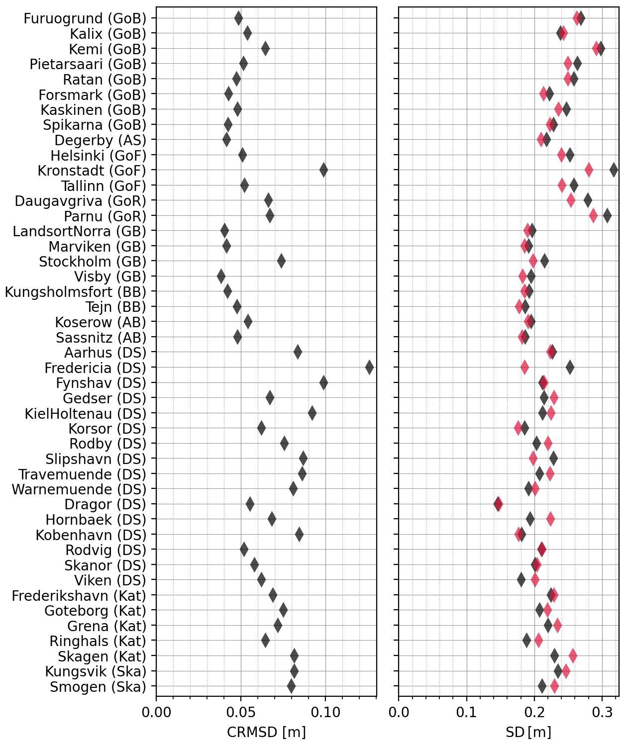
Figure 2 Sea surface height error metrics. Black and red symbols denote the model and observations, respectively. See Fig. 1 for station locations. Sub-basins are indicated by the following abbreviations: GoB, Gulf of Bothnia; AS, Archipelago Sea; GoF, Gulf of Finland; GB, Gotland basin; BB, Bornholm basin; AB, Arkona basin; DS, Danish Straits; Kat, Kattegat; Ska, Skagerrak.

In general, the model reproduces SSH standard deviation well (Fig. 2). The difference is within 2 cm in most cases; the largest deviation at Fredericia is approximately 7 cm. In the Baltic basin, the model has a tendency to overestimate variability. In the Danish Straits, the variability is slightly underestimated at several locations, although overestimation also occurs.

Figure 3 Taylor diagram of sea surface height error metrics. The metrics have been normalized by the standard deviation of the observations. See Fig. 1 for station locations; the sub-basin abbreviations are as in Fig. 2. NS stands for the North Sea.

The Taylor diagram (Fig. 3) shows that the model reproduces SSH variability well. Most stations have NCRMSD < 0.45, and the correlation coefficient is generally above 0.90. The agreement between the model and the SSH observations is generally higher in the open Baltic Sea than in Danish Straits. In the Baltic Sea, the NCRMSD is below 0.3 (except at Kronstadt and Stockholm) and the correlation coefficient is above 0.95 (except at Stockholm). In the Danish Straits, stations Fredericia, Kobenhavn, and Fynshav show much lower correlations below 0.9. This local drop in the performance is expected due to the complex bathymetry in the Danish Straits. Similarly, the lower performance at Stockholm is likely affected by the archipelago, which is not fully resolved in the model.

Figure 3 includes four tide gauges in the North Sea (gray symbols) where the tidal range is much larger. The tides are well reproduced (R > 0.94). Performance is the best at Aberdeen and Dover; at Helgoland, the performance is similar to the Kattegat–Skagerrak stations. Standard deviation is slightly underestimated.

3.2 Sea surface temperature and salinity

Sea surface temperature (SST) is mostly governed by surface heat fluxes, driven by the seasonal cycle of solar radiation and air temperature, and vertical mixing in the water column. In addition, near the coast (where tide gauges are located), riverine heat flux can cause local variations.

Figure 4 Surface temperature error metrics. Black and red symbols denote the model and observations, respectively. See Fig. 1 for station locations; the sub-basin abbreviations are as in Fig. 2.

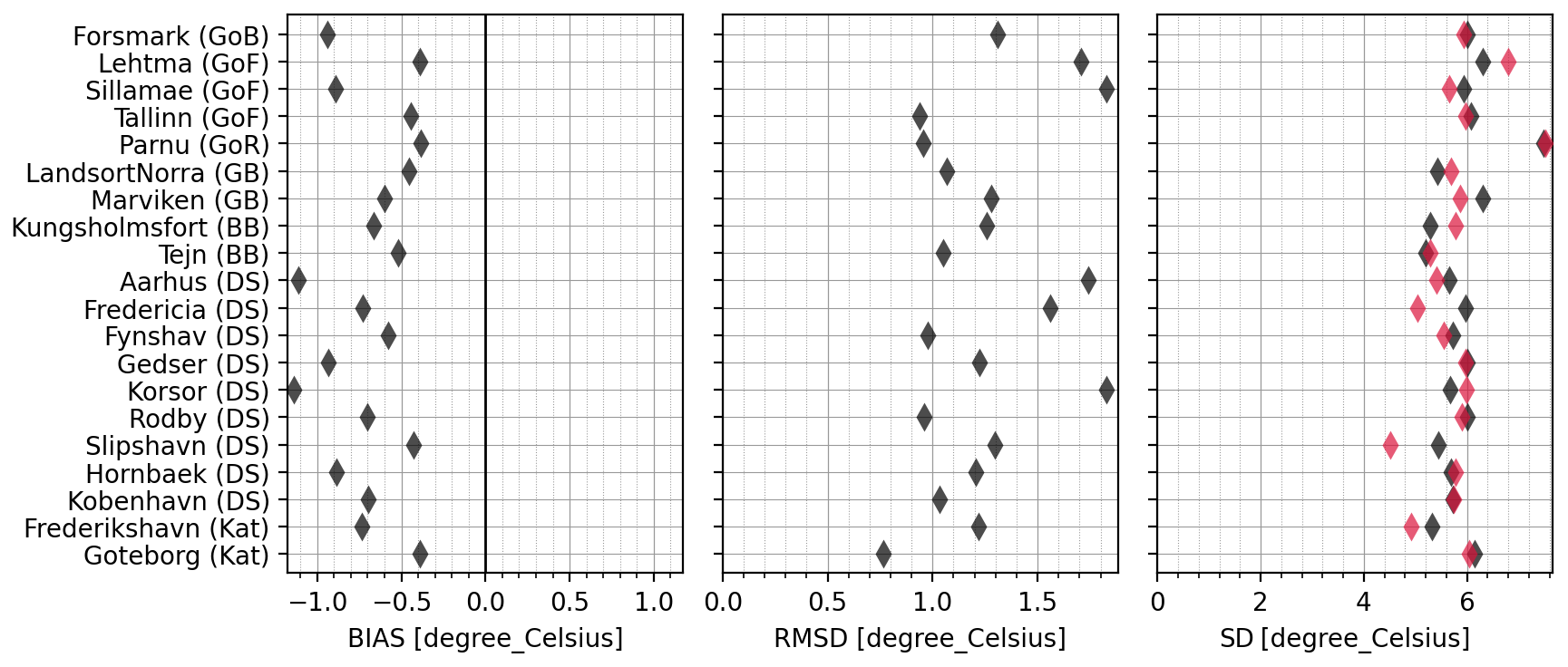
Tide gauge SST metrics are shown in Fig. 4. In general, there is no clear pattern across the domain. The model has a negative bias (typically between −0.4 and −0.9 ^∘C) at almost all stations; the largest bias (exceeding −1.1 ^∘C) occurs at Korsor. The RMSD is below 1.9 ^∘C in all cases. The standard deviation is typically close to the observed value.

Figure 5 Taylor and target diagram of surface temperature error metrics. The metrics have been normalized by the standard deviation of the observations. See Fig. 1 for station locations; the sub-basin abbreviations are as in Fig. 2.

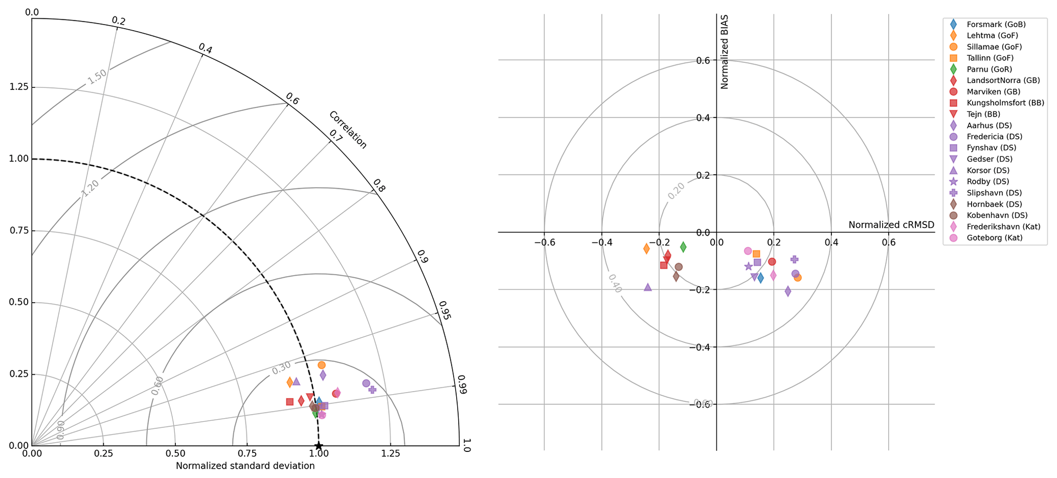
The Taylor diagram (Fig. 5, left) shows that SST skill is good in general. All locations are within 0.30 NCRMSD and have a correlation coefficient above 0.95. The normalized standard deviation is generally close to unity except at Fredericia and Slipshavn. The metrics indicate that the model captures the seasonal SST variability well. The normalized target diagram (Fig. 5, right) shows that the negative bias is quite small (typically NBIAS<0.20) compared to the overall SST variability (i.e., seasonal cycle).

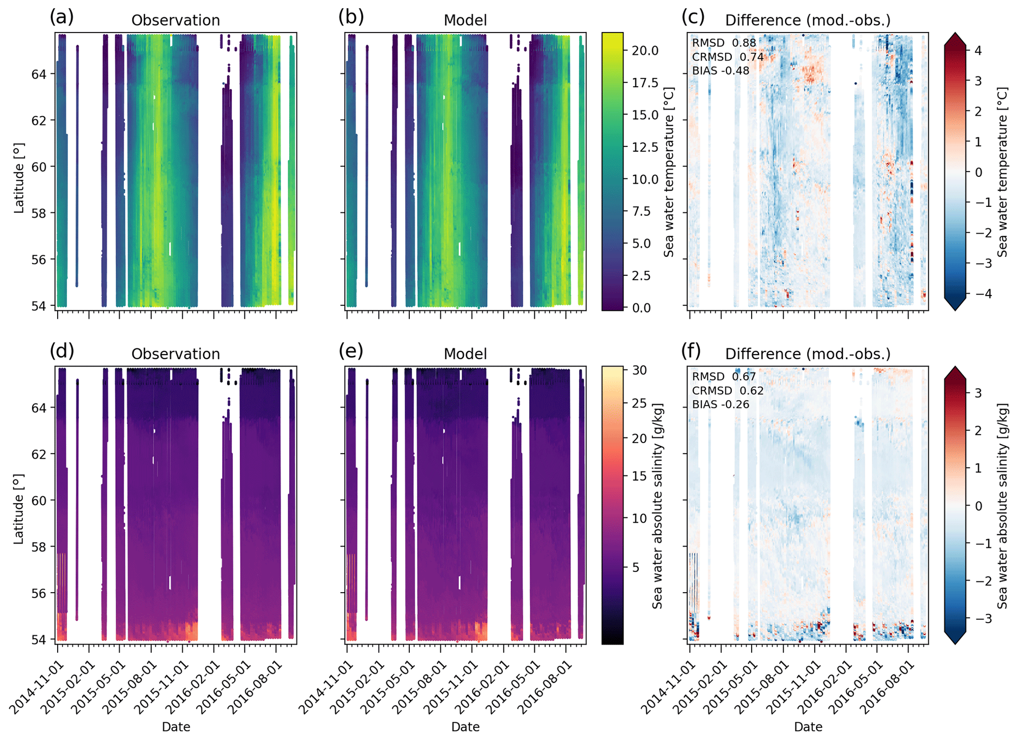
Figure 6 Surface temperature and salinity comparison against TransPaper FerryBox observations. The ferry operates between Oulu (a–c) and Lübeck (d–f; route is shown in Fig. 1b). At the beginning of the data set (November 2014) the ferry also visited Gothenburg.

Figure 7 Surface temperature and salinity comparison against FinnMaid FerryBox observations. The ferry operates between Helsinki (a–c) and Lübeck (d–f; route is shown in Fig. 1b).

Comparison against FerryBox SST from the TransPaper and FinnMaid ferries are shown in Figs. 6 and 7, respectively (top row). Although the FerryBox data have sparser temporal coverage than the tide gauge observations, they are useful for validating the modeled SST in open waters away from the coasts. The annual temperature cycle is also well reproduced here. The model bias is less than −0.5 ^∘C for the two ferries (Figs. 6c and 7c). RMSD is below 0.9 ^∘C, suggesting that SST performance is better in the open sea than at the tide gauge locations.

The TransPaper comparison shows a negative bias in the Baltic Proper and Gulf of Bothnia in summer 2015 (June–July; Fig. 6c). The bias is smaller during the following fall (October–December). A negative bias is visible in summer 2016 as well. The shorter FinnMaid data set also shows the negative bias during summer 2015 (Fig. 7c). Although the data coverage is sparse, the comparison suggests that the model has a negative bias during summer months (June–July), whereas the bias is smaller in fall. The magnitude of these deviations is, however, typically below 1.5 ^∘C.

FerryBox sea surface salinity (SSS) comparison is shown in Figs. 6 and 7 (bottom row). TransPaper observations (Fig. 6d) clearly show the SSS gradient ranging from roughly 15 g kg⁻¹ in the Belt Sea to 0 g kg⁻¹ in the northern part of the Bothnian Bay. In November 2014, the ferry also visited Gothenburg where SSS can reach 30 g kg⁻¹. The model reproduces the horizontal salinity gradient well; bias is −0.26 g kg⁻¹ and RMSD is 0.67 g kg⁻¹. In the FinnMaid data set (Fig. 7f), the bias and RMSD are similar at −0.16 and 0.55 g kg⁻¹, respectively. In both cases, the deviation is the largest in the Belt Sea and Kattegat where the model predominantly underestimates SSS. The larger error magnitude is due to the significant salinity gradients and their temporal variability in this region. The model has a small negative bias (−1 g kg⁻¹) in the Bothnian Sea (Fig. 6f). A negative bias is seen in the Gulf of Finland as well (around latitude 60^∘ N; Fig. 7f).

3.3 Vertical profiles

Figure 8 shows a comparison of temperature and salinity profiles against research vessel observations. In all panels, the outer ring denotes NRMSD, the middle ring RMSD, and the center dot the bias. RMSD and bias are visualized using the same color map; in all cases light color indicates small deviation. In addition, the metrics across all the plotted stations are printed in the upper left corner.

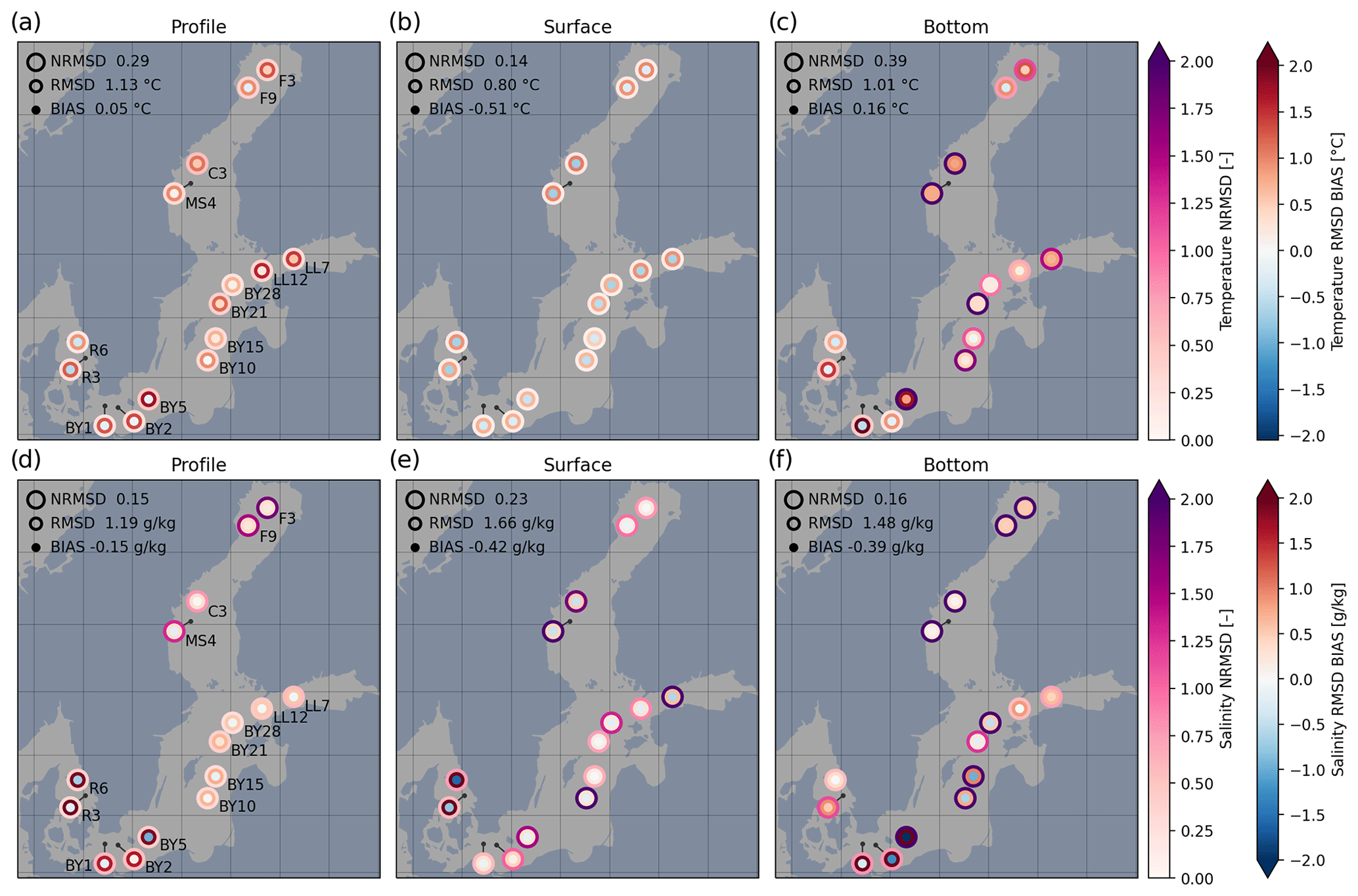
Figure 8 Vertical profile comparison against vessel observations; temperature (a–c) and salinity (d–f). The dots depict NRMSD (outer ring), RMSD (inner ring), and bias (center dot). The metrics have been calculated for the entire profile (a, d), surface 10 m (b, e), and bottom (c, f). Combined metrics over all the stations are printed in each panel. Bottom values were computed for the lowest 15 % of the water column.

The temperature profile metrics (Fig. 8a) are quite similar throughout the Baltic Sea. NRMSD is below 0.5 at all locations (except at C3 where NRMSD is 0.54), indicating good skill. The metrics for surface temperature (top 10 m; Fig. 8b) show low deviations. The NRMSD of the combined data set is 0.14 and bias is −0.51 ^∘C. The high surface temperature skill is consistent with SST results presented in Sect. 3.2: the model can capture the seasonal surface temperature variability driven by the solar radiation. Based on the SST and profile metrics, the model reproduces surface layer temperature well.

The bottom temperature skill is poorer (Fig. 8c). RMSD in the Gotland basin is quite low (below 0.5 ^∘C), while being higher in the Gulf of Finland and Gulf of Bothnia (0.6 to 1.3 ^∘C). In these regions, however, NRMSD exceeds a value of 2.0 at several stations. While RMSD is moderate, the deviation is significant compared to the low variability of bottom temperature. The bias tends to be positive in the Baltic basin and negative in Kattegat and the Arkona basin. The largest deviation occurs at BY1 where RMSD reaches 2.0 ^∘C.

The model reproduces salinity profiles relatively well (Fig. 8d). The deviation is small (RMSD < 0.73 g kg⁻¹) in the Gotland basin and Gulf of Finland. NRMSD is large in the Gulf of Bothnia due to the fact that salinity is low in this region as a result of riverine freshwater input. In contrast, in the Danish Straits and Kattegat NRMSD is small, while RMSD is relatively high (up to 1.9 g kg⁻¹) for the opposite reason: in this region, salinity regularly varies by more than 10 g kg⁻¹.

Surface salinity metrics (Fig. 8e) are generally similar to the whole profile metrics, except NRMSD is high in the Bothnian Sea, Gulf of Finland, and southern Gotland basin.

The bottom salinity metrics are presented in Fig. 8f. NRMSD regularly exceeds 2.0 in the Baltic basin because the variability of bottom salinity is small. A significant negative bias is visible in the Arkona basin and especially in the Bornholm basin; the bias is also negative in the Gotland basin. The deviation is moderate in Kattegat and the Gulf of Finland. While absolute deviation is small in the Gulf of Bothnia, NRMSD is large. In general, the results indicate that bottom salinity is underestimated in the Arkona, Bornholm, and Gotland basins. The skill is poorest in Bornholm (BY5). At this location, the model reproduces the halocline correctly but tends to underestimate bottom salinity. During the first simulated year the deviation is roughly −2 g kg⁻¹; after November 2015 it is −4 g kg⁻¹.

3.4 The 2014 major Baltic inflow event

A major Baltic inflow (MBI) event occurred in December, 2014. Mohrholz et al. (2015) divided the event into four phases: during the outflow period (7 November–3 December 2014) strong easterly winds pushed surface waters from the Baltic Sea to Kattegat, lowering the mean sea level at Landsort by 57 cm. After the winds ceased for a couple of days, the inflow period was characterized by strong westerly winds. The precursory period (3–13 December 2014) brought saline waters through the Sound and into the Belt Sea. On 13 December, the saline inflow had reached Darss Sill. At the buoy, the salinity exceeded 17 g kg⁻¹ in the entire water column, marking the beginning of the main inflow period. The main inflow period lasted until 25 December 2014 when the westerly winds, and hence the barotropic inflow, ceased. During this time, the mean sea level at Landsort rose 95 cm from the lowest value until the dense saline water mass had reached the Arkona basin. In the post-inflow period (starting on 25 December 2014), the saline water mass crept further into the Bornholm basin and the following downstream sub-basins driven by the baroclinic pressure gradient (density difference).

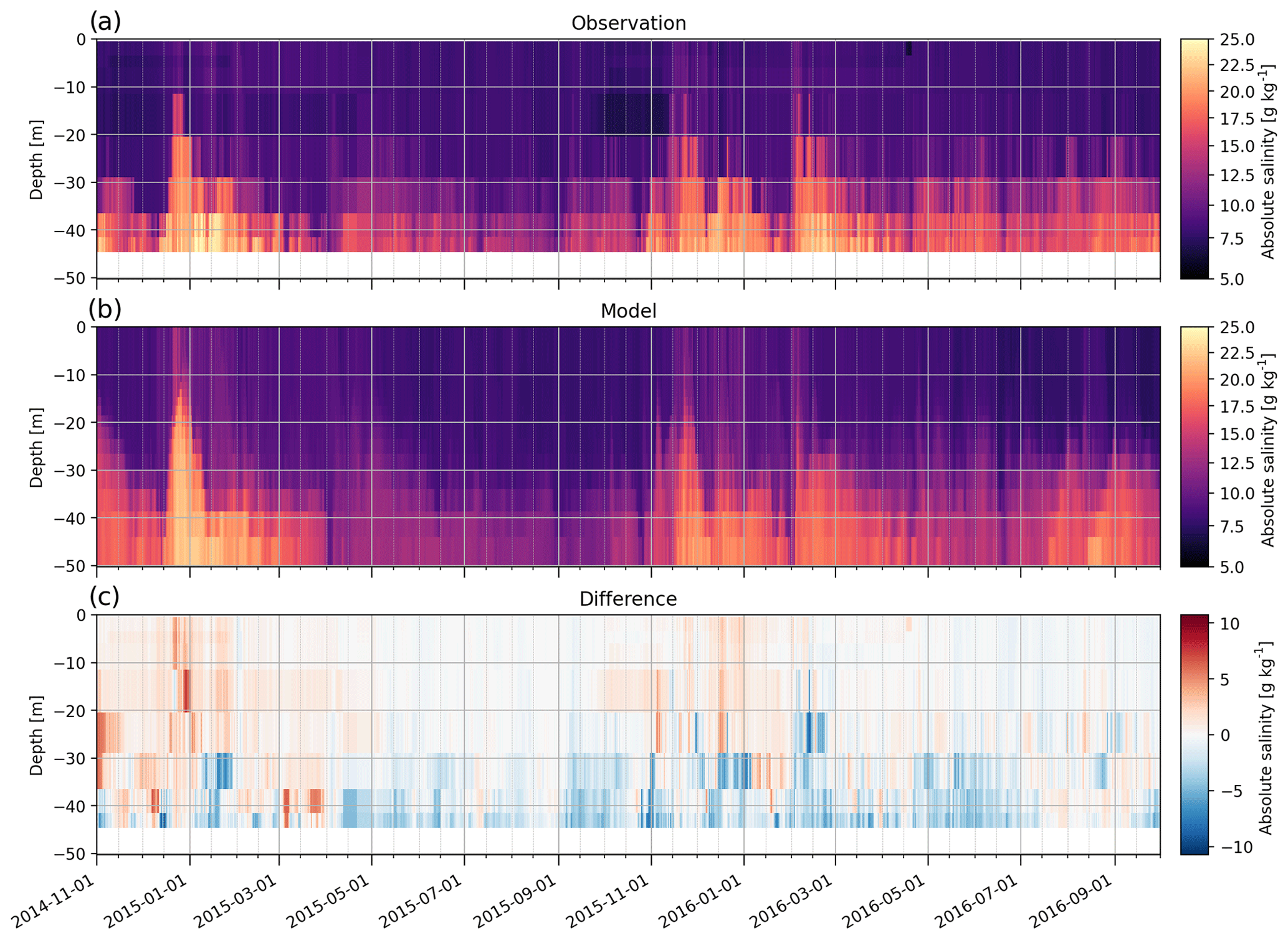
Figure 9 Vertical profile of salinity at Arkona. (a) Observations; (b) model; (c) difference (model minus observations). The difference field has been computed by interpolating the model data to the observation locations.

The observed salinity from the Arkona buoy is shown in Fig. 9a. The main salt pulse arrived at the buoy on 16 December 2014. On 20 December 2014, the dense water reached a depth of 16 m. The model replicates the arrival of the pulse on 16 December 2014 and the main inflow phase (20 to 26 December 2014; Fig. 9b). The bottom salinity is underestimated during the onset of the pulse (12 to 20 December 2014) from 4 January 2015 onward (Fig. 9c). Most notably, the observations show a secondary salt pulse in April 2015, which is underestimated in the model. The subsequent stronger pulses, in November 2015 and March 2016, are reproduced but their magnitudes are also slightly underestimated. In general, the model captures the MBIs but has a tendency to underestimate salinity at the bottom and overestimate it in the rest of the water column (up to a depth of 35 m).

Figure 10 Time series of bottom salinity at selected locations. The red line denotes the model, and the black dots are the observations.

A time series of bottom salinity at the Arkona buoy is shown in Fig. 10 (panel a), accompanied by observations at BY5 (Bornholm basin; panel b), BY10 (Gotland basin; panel c), and BY15 (Gotland deep; panel d). As stated above, the inflow reached Arkona on 16 December. The first observation of elevated salinity at BY5 is from 19 February 2015, but due to the gap in the measurements the pulse may have arrived earlier. At BY10 and BY15, an elevated bottom salinity is observed on 21 February and 17 March, respectively. The timing is quite well captured by the model: at Arkona the salt pulse is delayed by 1.5 d. The modeled salt pulse reaches BY5 at the end of December 2014, BY10 at the end of February 2015, and BY15 at the beginning of March 2015. The model underestimates the maximum bottom salinity by roughly 2.5 g kg⁻¹ at Arkona, 0.5 g kg⁻¹ at BY5, and 0.3 g kg⁻¹ at BY10. The deviation, however, increases in time at BY5, BY10, and BY15. At BY5, the observed salinity remains above 18 g kg⁻¹ (most of the time) after March 2015, while the modeled salinity decreases over time; in September 2016 the model underestimates salinity by 4 g kg⁻¹.

A similar decrease in modeled salinity, although smaller in magnitude, is also seen at BY10 and BY15. The observations show a subsequent increase in bottom salinity (in February and April 2016 at BY15 and BY10, respectively), but the model does not capture these events. In summary, the results indicate that the model does reproduce the magnitude and timings of the 2014 MBI event and its propagation into the Baltic Proper. It does, however, underestimate the bottom salinity by 1 to 4 g kg⁻¹ and does not reproduce lesser MBI events observed in 2015 and 2016. The negative salinity bias is also seen in the profile statistics (Fig. 8f).

3.5 Sea ice

Sea ice extent (defined as the total area where the sea ice area fraction exceeds 0.15) is presented in Fig. 11 for the winters 2014/2015 (panel a) and 2015/2016 (panel b). The winter 2014/2015 was exceptionally mild with only about 50 000 km² of sea ice extent, whereas the winter 2015/2016 was quite typical; the maximum ice extent of 120 000 km² was observed in January 2016. During both winters, the model tended to overestimate the ice extent by roughly 25 000 km². In relative numbers, the maximum ice extent was overestimated by 45 % and 25 % for the two winters, respectively. The ice season also started earlier in the model, especially in November 2014.

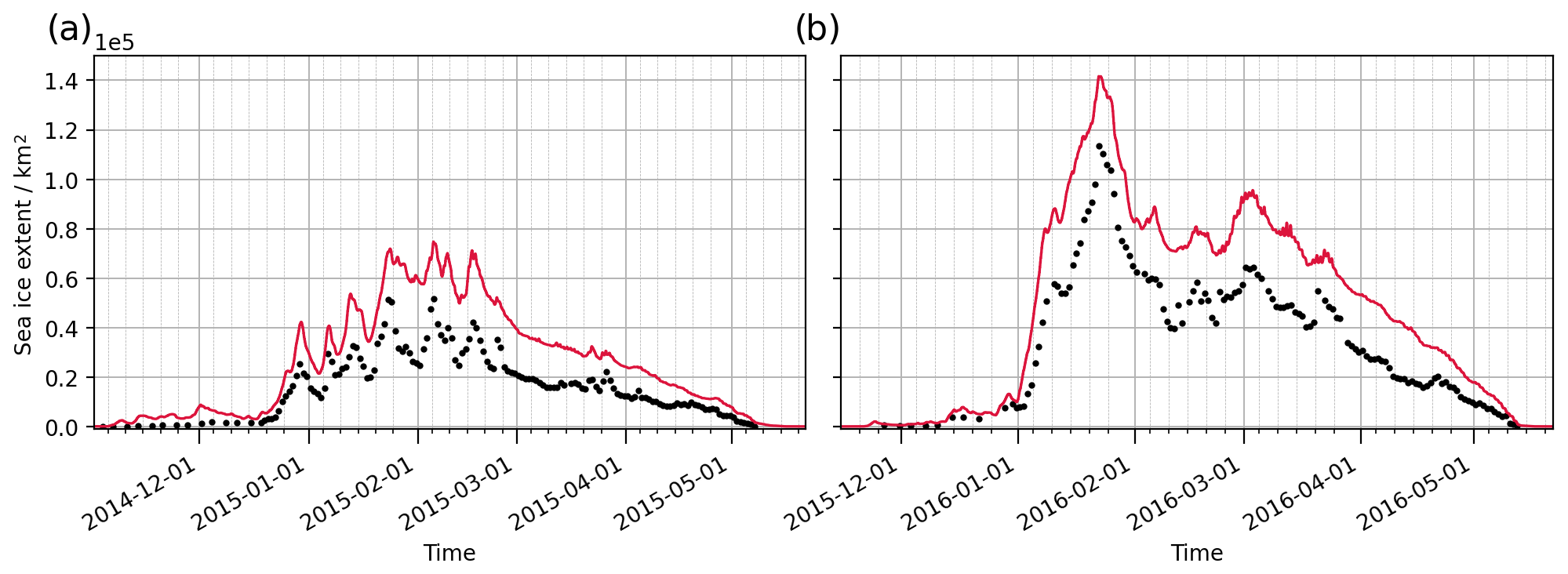
Figure 11 Time series of sea ice extent in the Baltic Sea for the two simulated winters. The red line denotes the model, and the black dots are the observations.

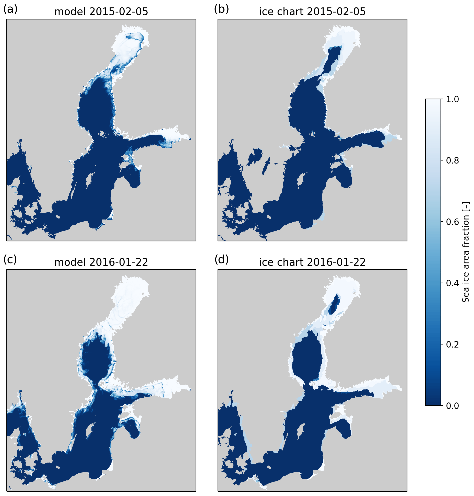
Figure 12 Comparison of sea ice area fraction from the model (a, c) and ice charts (b, d) for the maximal sea ice extent conditions in 2015 and 2016.

The spatial distribution of modeled sea ice is compared against FMI ice charts in Fig. 12. The dates shown correspond to the largest sea ice extent in the ice charts for winters 2014/2015 and 2015/2016. In both cases, sea ice is formed in the Bothnian Bay and eastern part of the Gulf of Finland. In the colder winter 2015/2016, ice coverage extends to the northern part of the Bothnian Sea, the Archipelago Sea, and the northern part of the Gulf of Riga. Generally, the modeled ice coverage agrees well with the ice charts. The most notable difference is the open-water area in the Bothnian Bay (Fig. 12b, d), which the model does not reproduce. The model has a tendency to form more ice near the coasts (e.g., along the coast of Sweden). The model field also shows larger areas with low (<0.4) sea ice area fraction, which may contribute to the larger extent seen in Fig. 11.

3.6 SSH under storm conditions

To assess how well the model is able to reproduce sea level variations under storm conditions, we analyze the Elon and Felix storms that occurred between 7 and 12 January 2015 (Fig. 13). The storms created strong westerly winds in the southern Baltic, with daily mean wind speed between 10 and 18 m s⁻¹. Figure 13 shows SSH time series at four stations in different parts of the Baltic Sea to illustrate the propagation of seiche oscillations.

Figure 13 Time series of sea levels at selected locations during the Elon and Felix storms. The red line denotes the model, and the black dots are the observations. The blue vertical lines indicate events discussed in the text. The model data have been bias-corrected for visual comparison.

On 8 January, westerly winds pushed water from the southern Baltic Sea to the east, lowering sea level in the Arkona basin and increasing it in the Gulf of Finland (event 1 in Fig. 13b, c); as the winds calmed, sea level at Helsinki retracted. The main storm event occurred on 10 January, when strong westerly winds pushed water from the North Sea to Kattegat (Fig. 13d). Initially, sea levels rose in the Arkona basin (event 2A in Fig. 13c), but as winds prevailed and moved to the east, sea levels dropped by roughly 1.5 m in 12 h (2B). This led to a sea level increase in the Gulf of Finland and the Bothnian Sea (2B in Fig. 13a, b). On 11 January, northerly winds pushed water to the south, causing an opposite sea level change (event 3). This was followed by another weaker westerly wind event (event 4).

Overall the model captured the wind-driven water elevation variations in the southern Baltic Sea. The extremes are slightly underestimated: the maximum observed and simulated SSH range at Rodvig are 1.68 and 1.55 m, respectively. At Ringhals the values are 1.40 and 1.27 m. The modeled seiche oscillations in Gulf of Bothnia and Gulf of Finland (Fig. 13a,b) are in good agreement with the observations. In Helsinki, the amplitude tends to be slightly overestimated, and there is a phase lag of 1 to 2 h. The tendency to underestimate SSH variability in the Danish Straits region and overestimate it in the Baltic basin agrees well with the results of long-term validation using tide gauge data (Fig. 3).

To assess how well the model captures high and low SSH events during the entire simulation period, we identified five highest and five lowest SSH extremes in each tide gauge time series. The corresponding maximum and minimum SSH levels were identified from the model within a 6 h window from the observation extremum. The model's deviations from the observed peak and through were then calculated. Prior to the analysis, mean SSH was removed from both the observation and model data. The results are summarized in Fig. 14.

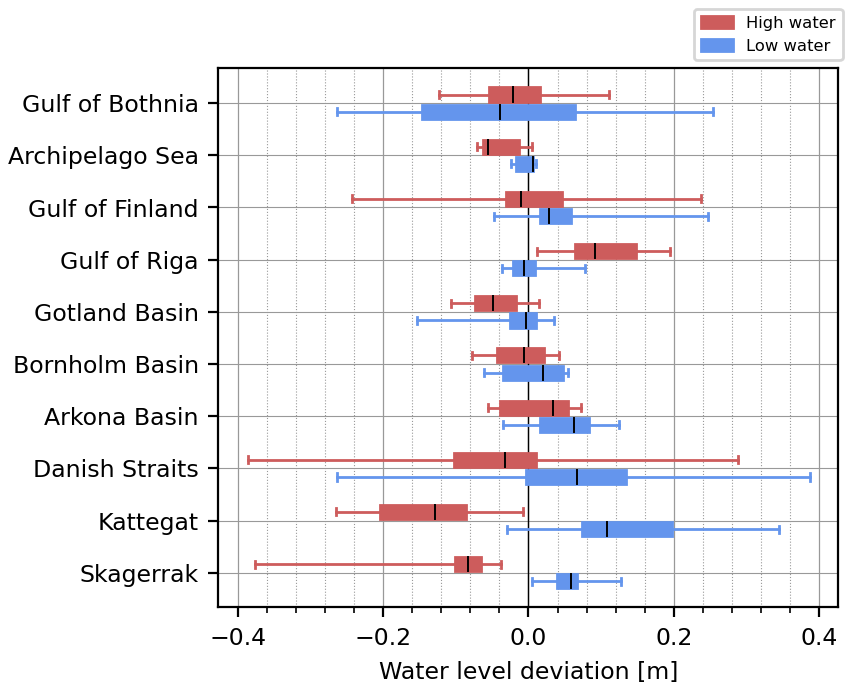
Figure 14 Model deviation in extreme water level cases in different sub-basins. Red and blue bars indicate the model's deviation from the observed SSH maximum and minimum, respectively. Positive values mean that the modeled SSH is higher. The thin line denotes the entire deviation range; thick bars indicate the 25th to 75th percentile range. The black line denotes the mean. The sub-basins are defined as in Fig. 2.

The model tends to underestimate high SSH values, especially in tidally dominated regions (Danish Straits, Kattegat, and Skagerrak). Low SSH values are similarly underestimated (i.e., positive deviation) in these regions. In general, the spread of the deviation is larger (up to 70 cm) in the tidally dominated regions, while being small in the deeper basins (within 20 cm). The spread is larger in the Gulf of Bothnia and Gulf of Finland due to SSH build-up in these elongated basins. High SSH events are overestimated in the Gulf of Riga. These results confirm that the model tends to underestimate SSH variability in the Danish waters, while it is slightly overestimated in the Gulf of Bothnia and Gulf of Finland.

4 Discussion and conclusions

The presented skill assessment for the 23-month period (1 November 2014–30 September 2016) shows that the model captures the main hydrographic features of the Baltic Sea. SSH variability is well reproduced. SSH skill is especially good in the Baltic basin: CRMSD is typically below 7 cm. In the Danish Straits region, the deviation is larger due to the interaction of the tides and the complex topography. The SSH metrics indicate that the tides propagate from the North Sea to Skagerrak and Kattegat without much loss of accuracy. SSH performance drops in the Danish Straits region, most likely due to insufficient horizontal resolution. It is worth noting that many tide gauges are located in harbors, river mouth regions, or small embayments that cannot be properly resolved at the resolution used. Under storm conditions, the model reproduces SSH dynamics well but has a tendency to underestimate the extremes. This is attributable to the atmospheric forcing data, which generally tend to underestimate extremes during storm events, as well as to the model's dissipation (e.g., caused by coarse grid resolution or friction parameterization).

The SST and SSS are generally well reproduced. In the FerryBox comparison, RMSD values were 0.9 ^∘C and 0.70 g kg⁻¹, respectively. SST, however, shows a systematic negative bias of approximately −0.5 ^∘C. Our calibration runs suggest that the negative SST bias can be related to underestimated vertical mixing. Another possible cause is river runoff temperature, which has a strong impact on SST in the vicinity of the river mouth. Yet another possibility is the downward longwave radiation forcing from the atmospheric model. Near the bottom, the temperature deviation is larger and RMSD can exceed 2 ^∘C. It should be noted, however, that due to the long residence time of the Baltic Sea (Döös and Engqvist, 2007), the bottom salinity and temperature in the presented simulation do depend on the initial conditions as well.

The modeled sea ice coverage is in good agreement with ice charts, but the model tends to overestimate the overall sea ice extent by 25 % to 45 %. As ice growth is strongly affected by SST, the overestimation is likely affected by the negative SST bias. Our calibration runs indicate that the sea ice model parameters have only a minor effect on the sea ice extent. Further research is needed to improve the biases in SST and sea ice.

The model replicates the 2014 MBI event and subsequent inflows in 2015 and 2016. The timing and magnitude of the MBI salt pulse at Arkona compare well with observations, and the bottom salinity is only slightly underestimated. In the Bornholm basin, the MBI is relatively well simulated by the model, especially considering that the initial bottom salinity is slightly low. After the inflow, however, the modeled bottom salinity decreases at a semi-constant rate and much faster than in reality. There could be several reasons for this. First, the vertical profile comparison (Figs. 9 and 10) suggests vertical mixing that is too high. It is possible that the vertical resolution is too coarse in the deeper layers (see discussion below), leading to high numerical diffusion. Second, the fast decline in bottom salinity could be due to an absence of smaller inflows after the MBI, which the model is not able to simulate well enough. Third, the type of vertical discretization employed in the model (z^* coordinates) is not so well suited to simulate dense bottom currents over rough topography, which may lead to a spurious vertical circulation (Dietze et al., 2014). Smoothing of the topography between the Arkona basin and the Bornholm basin may help in this respect.

The volume and propagation of the inflow can also be affected by the horizontal resolution: inflow through the Sound, for example, is significant, contributing 20 % to 30 % of the total volume (Mohrholz et al., 2015), yet it is difficult to resolve the narrow strait in operational models (Fischer and Matthäus, 1996; She et al., 2007; Gräwe et al., 2015b).

While both the Nemo-Nordic 1.0 and 2.0 versions use 56 vertical levels, their thickness distributions are different. In the 2.0 configuration, the surface resolution has been increased from 3 to 1 m in the top 10 m, implying coarser resolution between 50 and 200 m depths. Our calibration runs with 75 and 100 vertical levels indicate that higher vertical resolution in the 40 to 100 m range improves bottom salinity in the Bornholm basin (not shown). In addition, the strength of the salt inflow is sensitive to the bathymetry in the Danish Straits region (smoothing the bathymetry and deepening the channels), the advection schemes used (UBS for momentum advection), and turbulence closure parameters (lowering the Galperin limit). Thus, horizontal and vertical grid resolution, numerical mixing, and turbulence parameterizations all play important roles in simulating the inflow dynamics. MBI dynamics will be studied in more detail in the future.

From an operational modeling perspective, the presented model configuration delivers a sufficient performance that is generally comparable to other models (e.g., Meier et al., 1999; Burchard et al., 2009; Dietze et al., 2014; Hordoir et al., 2019). SSH skill is good in the entire Baltic basin. It is worth noting that in short-term forecasts the SSH skill is also highly dependent on the quality of the atmospheric forcing. SST and salinity biases are small or moderate, and those can be corrected with data assimilation. Surface currents are an important product of operational forecasts used in several applications, such as oil drift modeling. Validating modeled currents, however, is challenging due to the lack of measurements with sufficient spatial and temporal coverage. Comparing simulated currents at 1 nmi grid resolution against point measurements poses additional challenges (Lagemaa et al., 2010). Nevertheless, the model's ability to simulate SSH, water temperature, and salinity demonstrates that the general circulation and dynamics are captured fairly well even though direct validation of surface currents was not possible.

Improving the model skill is an ongoing effort. The bathymetry can be further improved to better represent the coastline and shallow coastal regions, as well as unresolved channels. The wetting and drying capability of NEMO (O'Dea et al., 2020) could improve SSH in shallow regions. Using higher vertical resolution will likely result in improved salt inflow dynamics. Further work is needed to calibrate advection schemes, diffusion parameterizations, and the representations of overflows to reduce numerical mixing. Most notably, adopting high-resolution nesting in strategic regions, such as the Danish Straits and the Archipelago Sea, could greatly improve the representation of water exchange processes. Finally, data assimilation and online coupling with atmospheric models can be used to further improve the modeling skill.