the Creative Commons Attribution 4.0 License.
the Creative Commons Attribution 4.0 License.
 | 10 Sep 2021
Efficient ensemble generation for uncertain correlated parameters in atmospheric chemical models: a case study for biogenic emissions from EURAD-IM version 5
Hendrik Elbern
Atmospheric chemical forecasts heavily rely on various model parameters, which are often insufficiently known, such as emission rates and deposition velocities. However, a reliable estimation of resulting uncertainties with an ensemble of forecasts is impaired by the high dimensionality of the system. This study presents a novel approach, which substitutes the problem into a low-dimensional subspace spanned by the leading uncertainties. It is based on the idea that the forecast model acts as a dynamical system inducing multivariate correlations of model uncertainties. This enables an efficient perturbation of high-dimensional model parameters according to their leading coupled uncertainties. The specific algorithm presented in this study is designed for parameters that depend on local environmental conditions and consists of three major steps: (1) an efficient assessment of various sources of model uncertainties spanned by independent sensitivities, (2) an efficient extraction of leading coupled uncertainties using eigenmode decomposition, and (3) an efficient generation of perturbations for high-dimensional parameter fields by the Karhunen–Loéve expansion.
Due to their perceived simulation challenge, the method has been applied to biogenic emissions of five trace gases, considering state-dependent sensitivities to local atmospheric and terrestrial conditions. Rapidly decreasing eigenvalues state that highly correlated uncertainties of regional biogenic emissions can be represented by a low number of dominant components. Depending on the required level of detail, leading parameter uncertainties with dimensions of 𝒪(106) can be represented by a low number of about 10 ensemble members. This demonstrates the suitability of the algorithm for efficient ensemble generation for high-dimensional atmospheric chemical parameters.
- Article
(12825 KB) - Full-text XML
- BibTeX
- EndNote


Due to highly nonlinear properties of the atmosphere, including its chemistry, forecast uncertainties vary significantly in space and time and among variables. During the last few decades, increasing effort has been put into estimating forecast uncertainties induced by different error sources. In this context, the method for generating an ensemble of forecasts is crucial as it determines the forecast probability distribution. While the represented details of the probability distribution increase with the number of realizations, the ensemble size of high-dimensional atmospheric systems is limited by computational resources (Leutbecher, 2019). Thus, the major challenge is the generation of ensembles that sufficiently sample the forecast uncertainty within manageable computational efforts. This renders ensemble forecasting one of the most challenging research areas in atmospheric modeling (e.g., Bauer et al., 2015; Buizza, 2019).
In numerical weather prediction (NWP), different ensemble methods have been developed in order to account for uncertainties of initial conditions and the forecast model formulation. First, studies were motivated by the fact that initial conditions induce dominant uncertainties to NWP systems. Bred vectors (BV, Toth and Kalnay, 1993) or singular vectors (SV, Buizza et al., 1993) are used to efficiently generate initial perturbations along the directions of the fastest growing errors in a linearized or nonlinear forecast model, respectively. Another approach estimates uncertainties of initial conditions by applying random perturbations to observations (PO, Houtekamer et al., 1996), which are assimilated into the modeling system.
As errors in initial conditions cannot entirely explain forecast errors, two methods related to uncertainties within the NWP model have been developed. Firstly, the stochastic kinetic energy backscatter scheme (SKEBS, Shutts, 2005) accounts for uncertainties in the amount of energy that is backscattered from subgrid to resolved scales. The second group of methods focuses on uncertainties in model parameterizations, which rely on simplified assumptions about non-resolved processes. In the stochastic parameter perturbation scheme (SPP, Houtekamer et al., 1996), selected parameters within individual parameterizations are multiplied with random numbers. In contrast, the stochastically perturbed parameterization tendencies scheme (SPPT, Buizza et al., 1999) considers uncertainties in the formulation of the parameterization schemes itself. Instead of perturbing individual parameters, total tendencies of state variables from all parameterizations are multiplied with appropriately scaled random numbers. Although perturbations are generated in a spatially and temporally correlated way, both correlation scales and standard deviations of the random numbers are predefined as fixed values (e.g., Leutbecher et al., 2017; Lock et al., 2019).
While different methods for ensemble generation are successfully applied to NWP, fewer approaches are available for chemistry transport modeling. As chemistry transport models (CTMs) include a large number of trace gases and aerosol compounds, the dimension of the system is even higher than in NWP (Zhang et al., 2012a). Among other implications, this high dimensionality amplifies the amount of uncertainties that differ significantly between individual chemical compounds (Emili et al., 2016). In the context of atmospheric data assimilation, reduced rank square-root Kalman filter approaches (Cohn and Todling, 1996; Verlaan and Heemink, 1996) have been successfully applied to reduce the high-dimensional covariance matrix to a small number of leading eigenmodes (e.g., Auger and Tangborn, 2004; Hanea et al., 2004; Hanea and Velders, 2007). Additionally, the temporal evolution of atmospheric chemical forecast errors differs from typical error growth characteristics in NWP. This inhibits a straightforward application of existing ensemble generation approaches from NWP to CTMs.
Besides using multi-model ensembles for estimation of forecast uncertainties (e.g., McKeen et al., 2007; Xian et al., 2019), there are only few attempts for ensemble generation within a single CTM. As CTMs are driven by meteorological forecasts, uncertainties in NWP are transferred to the chemical simulations. A comparably simple approach, which was used by Vautard et al. (2001) for the first time, employs an existing meteorological ensemble to drive the atmospheric chemical forecasts. However, estimations of chemical uncertainties solely driven by NWP ensembles do not necessarily represent related uncertainties in CTMs. For example, Vogel and Elbern (2021a) note that a global meteorological ensemble was not able to induce significant ensemble spread in near-surface forecasts of biogenic trace gases.
Multiple studies indicate that uncertainties of CTMs are mainly induced by uncertain model parameters – controlling emissions, chemical transformation, and deposition processes – rather than initial conditions or meteorological forecasts (e.g., Elbern et al., 2007; Bocquet et al., 2015). Consequently, former attempts aim to account for uncertainties in model parameters or other chemical input fields (for an overview, see Zhang et al., 2012b, and references therein). However, perturbing parameter fields appears to suffer from the high dimensionality of the system, as independent perturbations of model parameters at each location and time remain impractical. Early studies like the one performed by Hanna et al. (1998) assume predefined uncertainties where perturbations are applied uniformly in space and time, ignoring any cross-correlations between parameters. This uniform perturbation of model parameters with a fixed standard deviation is still applied to emissions in the context of ensemble data assimilation (e.g., Schutgens et al., 2010; Candiani et al., 2013).
However, constant perturbation of the whole parameter field does not allow for any spatial variation within the domain. More recently, limited spatial correlations are considered in uncertainty estimation by uniform perturbations within arbitrary sub-regions (Boynard et al., 2011; Emili et al., 2016) or isotropic decrease with fixed correlation length scales (Gaubert et al., 2014). Although recent approaches allow a local treatment of correlations, they are not able to represent the spatiotemporal properties of the dynamical system. Hanna et al. (1998) have already proposed that introducing state-dependent uncertainties and cross-correlations between parameters would provide a more realistic representation.
The Karhunen–Loéve (KL) expansion provides an opportunity to account for such complex correlated uncertainties based on eigenmode decomposition. While this approach is well established in engineering, it has rarely been applied in geophysical sciences. Siripatana et al. (2018) used the KL expansion for dimension reduction in an idealized oceanographic ensemble data assimilation setup. The eigenmode analysis required for the KL expansion is equivalent to a principal component analysis (PCA) by singular vector decomposition (SVD). The discrete PCA has been used as diagnosis tool in atmospheric sciences and is most established in climatology (e.g., Hannachi et al., 2007; Galin, 2007; Liu et al., 2014; Guilloteau et al., 2021). Goris and Elbern (2015) performed singular vector decomposition to determine optimal placement of trace gas observation sites. To the knowledge of the authors, the KL expansion has not been used for ensemble generation in atmospheric chemical models.
In order to address this issue, this study introduces a novel approach for optimized state-dependent parameter perturbation in atmospheric chemical models. The approach is based on the idea that the dynamical system induces multivariate correlations of model states and uncertainties. In particular, the algorithm aims to provide (1) an efficient assessment of various sources of uncertainties, (2) an efficient extraction of leading coupled uncertainties, and (3) an efficient generation of perturbations for high-dimensional parameter fields. Section 2 provides the concept of sensitivity estimation on which the ensemble generation approach is based. The specific algorithm presented in Sect. 3 is designed for model parameters that depend on model arguments like model inputs and configurations. Representative performance results are presented in Sect. 4 for biogenic emissions representing a highly uncertain (yet correlated) set of parameters. A discussion of the benefits and limitations of the presented approach is given in Sect. 5. Finally, Sect. 6 provides a summary and conclusions of this study.
This section introduces the conceptual basis for the description of the ensemble generation algorithm in Sect. 3. The algorithm relies on several definitions, which are introduced in Sect. 2.1. Given these definitions, the concept of sensitivities consists of two parts: the general formulation of sensitivities in Sect. 2.2 and the special formulation of independent sensitivities in Sect. 2.3. Each of these parts provides the basis for combined or independent covariance construction in the ensemble generation algorithm, respectively.
2.1 Definitions
The concept of sensitivity estimation requires the definition of several terms. This section introduces these terms on a general level and provides examples for the application to CTMs. All important terms used in the concept of sensitivity estimation and the algorithm are summarized in Table 1, including specific examples for the application to biogenic emissions.
Generally, the term “model parameter” refers to any parameter in the prognostic equations of the model that may affect the model forecast. A prominent example of a highly uncertain model parameter in CTMs is trace gas emissions. Considering multiple model parameters, like the emission rates of different trace gases, the dimension N of the problem is the total number of all considered parameters at all grid boxes. The total set of all parameter values at all grid boxes at time t is denoted by vector Q(t)∈ℛN. In the case of trace gas emissions, Q(t) includes the simulated emission rates of all considered gases at all grid boxes. Thus, the nth entry of the parameter vector is the simulated value of model parameter pn at grid box . The index specifies the model parameter and grid box and is therefore denoted as “position”. Hence, the positions of all parameters at all grid boxes is given by the index set .
The concept of sensitivities uses a set of J parameter vectors Qj(t) from differently configured model simulations . In this approach, different model simulations are achieved by using different implementations ri of a set of model arguments . The term “model argument” comprises a heterogeneous set of available arguments for the specific configuration of the model. In this regard, model arguments in CTMs may be as diverse as initial and boundary conditions, any external input fields, and the formulation of parameterizations in the model. The specific implementation ri of a model argument i is realized by selecting one available option of the argument in the model. For example, input fields of land surface properties may be one model argument with two implementations: land surface information from source A and from source B. In the concept of sensitivity estimation, each model argument is interpreted as an arbitrary parameter with Ri different implementations . Thus, each “setup index” represents a complete “model setup” as a specific combination of implementations ri of each model argument . Thus, is the parameter value of position s ∈ S simulated with model setup at discrete time . Note that the complete set of considers all possible combinations of implementations of all model arguments.
Table 1Notations used in the concept of sensitivity estimation and the formulation of the algorithm (including examples).

2.2 Formulation of sensitivities
The formulation of state-dependent sensitivities is based on Elbern et al. (2007), who demonstrated the suitability of amplification factors in the context of 4D variational optimization of emissions. Let j* be a “reference model setup” () representing the selected “reference implementation” of each model argument . Following this, the model parameter of model setup j at time t and position s is divided by its corresponding value from the reference configuration . The “sensitivity factor” is defined as temporal average of those over the time interval [t1,tT]:
Depending on the type of model parameter, the sensitivity factors may not be Gaussian distributed. This is especially true for parameters that are positive by definition, like emissions of trace gases. Analogous to emission factors in Elbern et al. (2007), sensitivity factors of emissions are assumed to be lognormally distributed. In this case, the sensitivity factors are substituted to normally distributed “sensitivities” in order to simplify their further treatment:
Since the definition of sensitivities refers to all possible combinations of implementations of all model arguments, the set of is also denoted as a set of “combined sensitivities”. Given Ri implementations of each model argument , the total number of combined sensitivities with is
For atmospheric model parameters, each sensitivity requires its own forecast simulation. Thus, the calculation of all combined sensitivities becomes computationally demanding even for a low number of implementations of a few model arguments. Figure 1 shows the exponential increase of the number of combined sensitivities as function of the number of implementations and arguments from Eq. (3). For example, considering six model arguments (I=6) with two implementations each (), requires model executions prior to the ensemble generation.

2.3 Formulation of independent sensitivities
As this study aims for a computationally efficient algorithm focusing on leading uncertainties, the computational efforts required for the estimation of sensitivities are critical. Thus, a new method for efficient sensitivity estimation is introduced, which reduces the number of required model executions prior to ensemble generation significantly. Instead of using all possible combinations of model arguments, the method uses only sensitivities with respect to single model arguments. By assuming tangent linearity of sensitivities in the limits of imposed perturbations, these sensitivities are extrapolated to approximate the full set of combined sensitivities.
The assumption of tangent linearity equals mutual independence of the model arguments, and thus every combined sensitivity factor with arguments can be decomposed into a set of “independent sensitivity factors” for each single argument ri with
Here, the independent sensitivity factors are defined analogously to Eq. (1) using the model forecast
, where only one argument ri differs from the reference setup
Further, with Eq. (2), every combined sensitivity of implementation j at position s is given by
where is the independent sensitivity, referring to a single modified model argument with implementation ri. Note that the independent sensitivity factors equal 1 when the implementation ri of model argument i equals the reference implementation (analogous to Eq. 1). Consequently, the independent sensitivities vanish in Eq. (6) for all i with , and each combined sensitivity is given by the sum of independent sensitivities to those arguments, which differ from the reference setup
In other words, the assumption of independence implies that the set of all combined sensitivities lies within a subspace that is spanned by the set of independent sensitivities . Following this, the full set of combined sensitivities can be approximated by the subset of independent sensitivities following Eq. (7). This reduces the number of required forecasts from to
with , as shown in Fig. 1. Thus, the independent method requires a significantly reduced number of simulations, one for the reference setup () and one for each other implementation of each argument . For example, considering I=3 model arguments with Ri=5 implementations each, the total number of combined sensitivities reduces to independent sensitivities. For I=10 model arguments with Ri=2 implementations each, the number of required sensitivities can even be reduced by 2 orders of magnitude (Jindep=11, Jcombi=1024).
While the number of required simulations is considerably reduced, the underlying assumption of independent sensitivities disregards nonlinear interactions between different model arguments. A discussion of this assumption for the application to atmospheric model parameters is given in Sect. 5.
This section provides the description of the ensemble generation algorithm with respect to correlated model parameters. Here, a model parameter may be any parameter in the prognostic equations of the model state variables (compare Sect. 2.1). Making use of the Karhunen–Loéve (KL) expansion, the approach is hereafter denoted as the “KL ensemble generation approach”. It is based on the fact that the forecast model acts as a dynamical system, forcing spatial and multivariate couplings of the atmospheric state. Thus, information on the size and coupling of forecast uncertainties can be extracted from differently configured model simulations. The configurations of the model simulations is selected by the user according to sources of uncertainties of the selected model parameters. For recurring applications of the ensemble generation algorithm, the selection may also be guided by results of previous applications of the algorithm.
The explicit algorithm presented here focuses on state-dependent model parameters that depend on the specific model setup. Generally, atmospheric models are sensitive to their specific simulation setup, including a large variety of model inputs and configurations like initial and boundary conditions, external input data, and the selection of parameterization schemes in the model. Although comprising a highly heterogeneous set, all model inputs and configurations determining the specific simulation setup are henceforth denoted as model arguments. For state-dependent parameters considered here, their sensitivities to the model setup are assumed to induce dominant uncertainties. Thus, the problem of estimating multivariate uncertainties is transferred to sensitivities to the model setup.
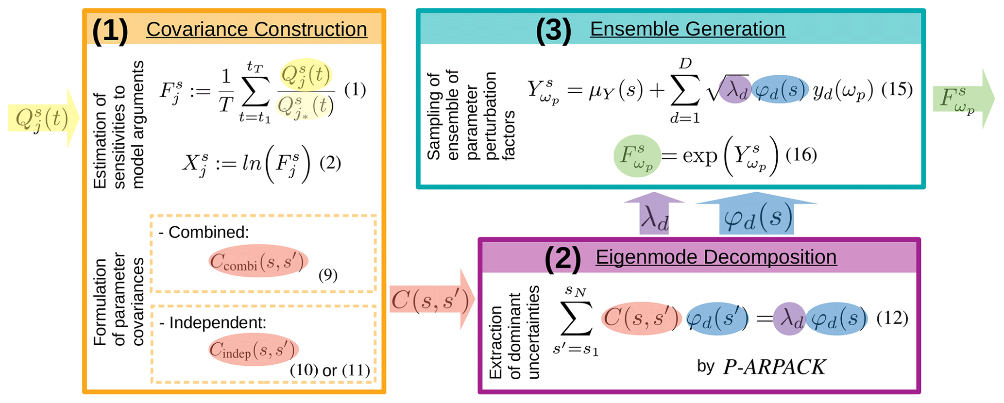
The algorithm consists of three major steps, which are described in the following: the construction of parameter covariances from combined or independent sensitivities (Sect. 3.1), the extraction of leading uncertainties using highly parallelized eigenmode decomposition software (Sect. 3.2), and the ensemble generation by sampling perturbations from leading eigenmodes with the Karhunen–Loéve expansion (Sect. 3.3). A graphical overview of the major steps composing the algorithm is given in Fig. 2. The formulation of the algorithm is based on the concept of sensitivity estimation introduced in Sect. 2; an overview over the terms used in this section is given in Table 1.
3.1 Covariance construction
As a first step, essential uncertainties of the model parameters are formulated as multivariate covariance matrix , where N is the dimension of the problem, i.e., the total dimension of the set of considered model parameters. Generally, the covariances may be determined from any kind of uncertainty, such as statistical model errors derived from operational forecasts. Because this study focuses on state-dependent parameters, essential uncertainties are estimated from sensitivities of those parameters to different model arguments. These state-dependent sensitivities are realized as temporally averaged sensitivity factors with respect to a selected reference as described in Sect. 2. The temporal averaging makes the sensitivities representative for a sufficient time interval for ensemble simulation. Generally, the covariance matrix should represent the complete set of essential uncertainties of the model parameters. Focusing on uncertainties induced by sensitivities to various model arguments , essential uncertainties can be estimated from different implementations ri of each model argument i. Ideally, the covariance matrix is calculated from the sensitivities to all possible combinations of various implementations of each argument (compare Sect. 2.2). In this case, the “combined covariance” between sensitivities at positions is given by
give the mean value of combined sensitivities at position s and s′, respectively.
If the assumption of independent sensitivities is applied, covariances are calculated from the set of independent sensitivities (compare Sect. 2.3). Rather than approximating all combined sensitivities from independent sensitivities explicitly, the effects on mean sensitivities and covariances are derived in their general from in Appendix A.
In the KL ensemble generation algorithm, the mean values μindep(s) and covariances of the sensitivities are directly calculated from the set of independent sensitivities by
Note that the assumption of independence does not imply orthogonality between the input sensitivities. While the equations are exact under the given assumption of tangent linearity, this assumption might be a strong limitation for many atmospheric processes.
The method of independent sensitivities allows the inclusion of additional uncertainties in a straightforward way. These additional uncertainties may originate from any other error source not represented as model arguments. For example, this could be a known uncertainty in the formulation of the model itself. If such an “additional uncertainty” is given (e.g., from statistical evaluation), it can be included as additional sensitivity with Radd=2. Based on Eqs. (10a) and (10b), the independent mean and covariance including additional uncertainties are
If the direction of the additional uncertainty is unknown (“unsigned additional uncertainty”), the original definition of the mean values for independent sensitivities as given in Eq. (10a) is used instead of Eq. (11a). This ensures no impact from the additional uncertainty on the mean values of the parameters.
3.2 Eigenmode decomposition
Once the multivariate covariances are formulated, dominating directions of uncertainties are extracted as a second step. This extraction is realized by an eigenmode decomposition of the covariance matrix
with λd the dth eigenvalue and the th element of the corresponding eigenvector φd∈ℛN for all with . As the presented approach focuses on dominant uncertainties, the D largest eigenvalues and corresponding eigenvectors are required with D<N. Here, the first eigenvalues represent the size of the most dominant uncertainties, and the corresponding eigenvectors represent their directions. Due to the high dimensionality of atmospheric models, the covariance matrix may easily be of the order of 1010 elements. This inhibits explicit storage of the matrix and makes the computation of the eigenproblem Eq. (12) very costly even for a low number of required eigenmodes (D≪N). Therefore, highly efficient software is required that is suitable for high-dimensional systems.
The ARPACK (ARnoldi PACKage, Lehoucq et al., 1997) package is a flexible tool for numerical eigenvalue and singular value decomposition. It is explicitly developed for large-scale problems and includes a set of specific algorithms for different types of matrices. The ARPACK software uses a reverse communication interface where the matrix needs to be given as operator acting on a given vector. ARPACK makes use of the implicitly restarted Arnoldi method (IRAM, Sorensen, 1997) which is based on the implicitly shifted QR algorithm. As a covariance matrix is quadratic, symmetric, and positive definite by construction, the IRAM method reduces to the implicitly restarted Lanczos method (IRLM). In this study, the parallel version P-ARPACK is used for the eigenmode decomposition, which balances the workload of processors and reduces the computation time. For a detailed description of the ARPACK software package, see Lehoucq et al. (1997).
3.3 Ensemble generation
The final step is the generation of an ensemble of perturbations based on the leading eigenmodes of parameter uncertainties. This step makes use of the Karhunen–Loéve expansion – denoted as “KL expansion” hereafter – named after Karhunen (1947) and Loéve (1948). The KL expansion provides a mathematically optimal combination of the dominant directions of parameter uncertainties given by the leading eigenmodes. The following description is adopted from the notations of Schwab and Todor (2006) and Xiu (2010), to which the reader is referred for more details. In its discrete form, the KL expansion describes the sth element of a stochastic process of dimension N as a linear combination of orthogonal components
with μ(s) denoting the mean value of the stochastic process and ωp its pth random realization. Here, the deterministic fields ψd(s) are given by the eigenvalues λd and eigenvectors φd of the covariances of the stochastic process
In this notation, the stochastic coefficients yd(ωp) are independent random numbers with zero mean and unit standard deviation.
In the context of ensemble generation, the stochastic process is a set of perturbations whose essential uncertainties are formulated as covariance matrix of the sensitivities as defined in Sect. 3.1. Thus, the eigenvalues λd and corresponding normalized eigenvectors φd(s) are provided by the eigenmode decomposition in Sect. 3.2. Normally distributed sensitivities can be realized by centered and normally distributed stochastic coefficients yd(ωp).
Using the KL expansion for ensemble generation, multivariate covariances induce coupled perturbations of the set of considered parameters. The higher the correlations of the sensitivities, the faster the decrease of the eigenmodes and the more the perturbations are determined by a few leading orthogonal components. Truncating Eq. (13) at D<N, the resulting KL approximation provides an optimal approximation of the stochastic process in the least-squares sense (Schwab and Todor, 2006). For ensemble generation, a set of D stochastic coefficients is randomly sampled for each ensemble member p from a normal distribution with zero mean and unit standard deviation. Given the set of leading eigenvalues and corresponding normalized eigenvectors , the perturbation of ensemble member at position s ∈ S is sampled from
Finally, the ensemble of perturbations is transferred back to a set of perturbation factors . If the model parameters are assumed to be lognormally distributed, a re-substitution as counterpart to the logarithmic substitution in Eq. (2) is performed
These perturbation factors will then be applied to the model parameters in the ensemble forecast.
Using the KL expansion for ensemble generation instead of singular vectors has one important advantage. In SV-based ensemble generation approaches, each perturbation is generated by one singular vector scaled by its singular value. Using the KL expansion, each perturbation is sampled from the series of eigenmodes using different random numbers for each perturbations. This allows for a flexible selection of the number of perturbations depending on the desired level of detail. Independent of the number of perturbations, the KL expansion ensures an optimal estimation of the largest uncertainties by the calculated perturbations.
This section provides results of the KL ensemble generation algorithm for an application to biogenic emissions in a regional CTM system. The modeling system used for the calculation of sensitivities and the specific setup of the algorithm are described in Sect. 4.1 and 4.2, respectively. Based on these, the results are presented with respect to two main objectives. Firstly, the behavior of the algorithm is illustrated for two different setups using combined and independent sensitivities, respectively. Sect. 4.3–4.5 present the results for each of the three major steps of the algorithm as described in Sect. 3. The description focuses on similarities between the two methods rather than on the detailed description of specific patterns. For the setup of independent sensitivities, additional uncertainties are included as described in Sect. 4.2 to demonstrate the inclusion of those. Secondly, the performance of the algorithm is evaluated for the two different setups. A comprehensive a posteriori evaluation would ideally be based on a representative amount of data covering multiple conditions. However, observations of biogenic gases are rare and only provide information on local concentrations and not on their emissions themselves. As concentrations are affected by other uncertain processes, an ensemble of emissions or emission factors produced by the algorithm cannot be evaluated by observations alone. Therefore, Sect. 4.6 evaluates the performance of the algorithm in terms of ensemble statistics.
4.1 Modeling system
The KL ensemble generation algorithm was implemented in a way that it uses precalculated output from the EURAD-IM (EURopean Air pollution Dispersion – Inverse Model) chemical data assimilation system. Note that the algorithm is independent of the forecast model, which can be replaced by any other CTM.
EURAD-IM combines a state-of-the-art chemistry transport model (CTM) with four-dimensional variational data assimilation (Elbern et al., 2007). Based on meteorological fields precalculated by WRF-ARW (Weather Research and Forecasting – Advanced Research WRF, Skamarock et al., 2008), the Eulerian CTM performs forecasts of about 100 gas-phase and aerosol compounds up to lower stratospheric levels. In addition to advection and diffusion processes, modifications due to chemical conversions are considered by the RACM-MIM chemical mechanism (Regional Atmospheric Chemistry Mechanism – Mainz Isoprene Mechanism, Pöschl et al., 2000; Geiger et al., 2003). Emissions from anthropogenic and biogenic sources, as well as dry and wet deposition, act as chemical sources and sinks, respectively. In this study, the EURAD-IM system provides forecasts of sensitivities to various model arguments, which are used for covariance construction in the KL algorithm. The concept of emission factors used for emission rate optimization in EURAD-IM was adapted in the KL ensemble generation approach as described below.
The KL ensemble generation algorithm is tested for biogenic emissions, which are known to be subject to large uncertainties. The MEGAN 2.1 model developed by Guenther et al. (2012) calculates biogenic emissions of various compounds in EURAD-IM as a function of atmospheric and terrestrial conditions including radiation, air temperature, leaf area index, and soil moisture. In this study, biogenic emissions of five dominant volatile organic compounds (VOCs) are perturbed: isoprene, limonene, alpha-pinene, ethene, and aldehydes. Note that biogenic aldehyde emissions from MEGAN 2.1 represent the total emission from acetaldehyde and a set of higher aldehydes that are not treated individually (see Guenther et al., 2012, for further details). Due to a collective approach in MEGAN 2.1, the biogenic emissions of different compounds are assumed to be highly correlated. Thus, the set of five biogenic emission fields is selected in order to investigate the joint perturbation of highly uncertain (yet correlated) parameters. In the KL algorithm, sensitivities from the five emission fields induce multivariate covariances in the covariance matrix C that allow for joint perturbation. The following description of the results focuses on emissions of isoprene, which is the most abundantly emitted biogenic trace gas.
4.2 Setup
In the KL algorithm, sensitivities used for covariance construction are taken from a case study covering the Po valley in northern Italy on 12 July 2012. A preceding study by Vogel and Elbern (2021a) demonstrated that local emissions of biogenic volatile organic compounds (BVOCs) are highly sensitive to various model arguments during this case study. At the same time, these sensitivities are found to be almost species invariant and show little variation on an hourly timescale, which allows for a generalized formulation of perturbations. Providing an appropriate test case, the sensitivities used in this study are based on the results of Vogel and Elbern (2021a), which have been simulated by EURAD-IM.
Specifically, emission sensitivity factors are calculated from hourly biogenic emissions divided by the corresponding reference emissions and averaged over the period from 00:00 until 10:00 UTC on 12 July 2012 according to Eq. (1). Here, minimum emissions of kg (km2 h)−1 are defined and sensitivity factors are limited by 0.1 and 10.0 in order to avoid unrealistic perturbations in regions of low emissions. As biogenic emissions are restricted to terrestrial vegetation, only land surface grid boxes are used, which reduces the total dimension of the problem by about 27 % compared to all surface grid boxes.
Two different implementations are selected for each argument (), where the reference is the default configuration of EURAD-IM and ri=2 are the alternative implementations of each argument i. Figure 3 shows 32 combined sensitivity factors of biogenic emissions calculated from EURAD-IM using Eq. (1) with different combinations of model configurations as listed in Table B1. For computational reasons, the subset of Jcombi=32 combined sensitivities is sampled from a total number of possible combinations. A detailed discussion of the origin of sensitivity factors used in this study is given in Vogel and Elbern (2021a). The selection of 32 combined configurations is based on the importance of the source of uncertainties reported there.
In contrast to the large amount of calculations required for combined sensitivities, the method of independent sensitivities is additionally investigated. As described in Sect. 2.3, only sensitivities resulting from the change of a single model argument are required for this method. This allows for an additional consideration of two uncertainties related to the emission model. These uncertainties are selected to demonstrate the inclusion of additional uncertainties in order to provide a most realistic setup of the ensemble for biogenic emissions. Firstly, the highly variable response of biogenic emissions to soil dryness is added to the set of independent sensitivities. This sensitivity is defined as the change of emissions when the drought response used in MEGAN2.1 is excluded (compare Vogel and Elbern, 2021a). Secondly, Guenther et al. (2012) indicate an uncertainty of the emissions model itself of 200 %, which is included as unsigned additional uncertainty (denoted as a priori uncertainty) with a constant factor of two for all locations and trace gases. Note that an unsigned additional uncertainty does only apply to the covariances given by Eq. (11b) and does not affect the calculation of the independent mean given by Eq. (10a). The formulation of a constant factor induces a simple assumption representing perfectly correlated errors in this case, but it is assumed to be sufficient to show the effect of including unsigned additional uncertainties in the algorithm.
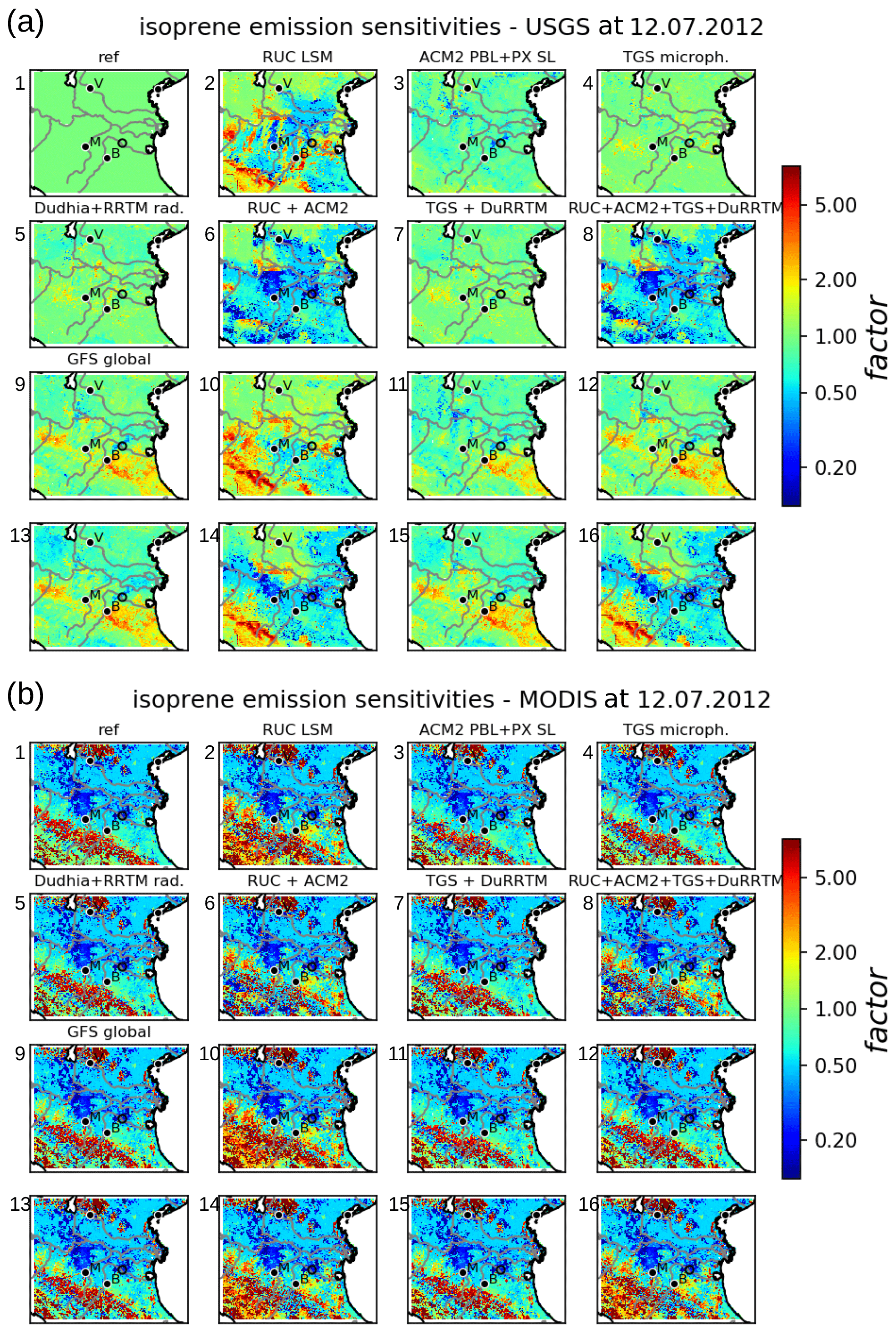
Figure 3Set of combined sensitivities of isoprene emissions. Shown are isoprene emission factors for different combinations of model arguments as simulated by EURAD-IM. Emission factors are temporally averaged ratios of emissions divided by the reference emissions. The specific setup used for each of the 32 sensitivities is given in Table B1. The sensitivities are divided into those using USGS (a) and MODIS (b) land use information; numbers attached to the individual subplots refer to the numbers in Table B1. In addition, a short abbreviation of the setup is given above each subplot. See also Vogel and Elbern (2021a) for a detailed description of the abbreviations and model implementations. Some major cities (Verona, Bologna, Modena) are indicated by their initial letters.
4.3 Sensitivity estimation
According to the definition in Eq. (1), sensitivity factors of the reference run (subplot 1 of Fig. 3a) are equal to 1 by definition. The set combined sensitivities is dominated by effects of land use information shown in Fig. 3b, inducing reduced or increased emissions in the mountains and the Po valley, respectively. As discussed in Vogel and Elbern (2021a), these large sensitivities in biogenic emissions are caused by different fractions of broadleaf trees in USGS land use information and MODIS data. Significant effects are also found with respect to global meteorology, land surface model (LSM), and boundary layer schemes. Here, weak nonlinear effects appear when RUC LSM is combined with the ACM2 boundary layer scheme or GFS global meteorology (subplot 6 and 10 of Fig. 3a).
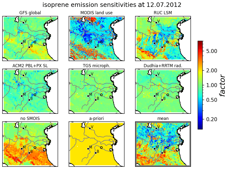
Figure 4Set of independent sensitivities of isoprene emissions simulated by EURAD-IM. Shown are isoprene emission factors of simulations where only one model argument differs from the reference setup. Plotting conventions including abbreviations as in Fig. 3. Additional uncertainties refer to the drought response (no SMOIS) and the emission model (a priori) of biogenic emissions. The lower-right subplot shows the independent mean from these sensitivities using Eq. (10a). A detailed description of the abbreviations and model implementations is provided by Vogel and Elbern (2021a).
Figure 4 shows the independent mean factors and sensitivities for isoprene emissions. Note that independent sensitivities are formulated relative to the independent mean, which are both limited by 0.2 and 5 to be consistent with the configuration for combined sensitivities. Similar to the results of combined sensitivities, MODIS land use information and the RUC land surface model produce significantly reduced isoprene emissions within the northern Po valley. The added sensitivity to drought response points towards increased emissions in the southern part of the domain. Consequently, the independent mean is dominated by reduced emissions in the northern part and increased values in the southern part. The a priori uncertainty of the emission model is represented by a constant factor of 2 and does not affect the independent mean by definition. The remaining independent sensitivities produce only minor deviations in biogenic emissions of all trace gases including isoprene.
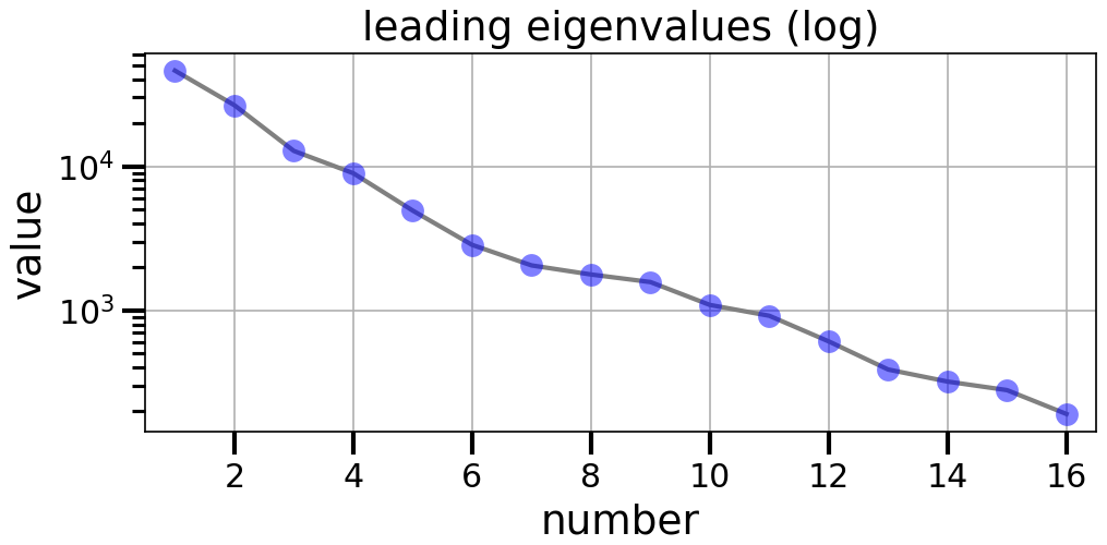
Figure 5Leading eigenvalues of biogenic emissions for combined sensitivities (blue dots). Eigenvalues are plotted on a logarithmic scale.
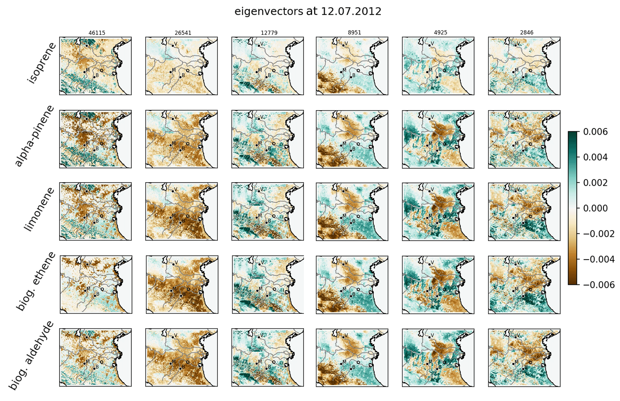
Figure 6Leading eigenvectors for combined sensitivities. The normalized eigenvectors are visualized as column of fields of different biogenic gases. Numbers above each column show the eigenvalues of the corresponding eigenvector.
4.4 Eigenmode decomposition
Based on the respective formulation of combined or independent sensitivities, the leading eigenvalues and their associated eigenvectors of the covariance matrices are calculated as described in Sect. 3.2. For combined sensitivities, the eigenvalues given in Fig. 5 show a logarithmic decrease of about 1 order of magnitude within the first five modes. This indicates that the major uncertainties of the emissions factors are determined by a few leading directions. In other words, the fast decrease of leading eigenvalues confirms a high correlation of biogenic emissions through the domain and between different gases. The contribution of these leading eigenmodes to local emission factors for each trace gas is given by the corresponding eigenvectors shown in Fig. 6. According to shape and size of the first eigenmode, it is almost exclusively induced by the sensitivity to land use information that is invariant to the other sensitivities. The subsequent eigenmodes represent common patterns of the remaining sensitivities that are therefore treated together.
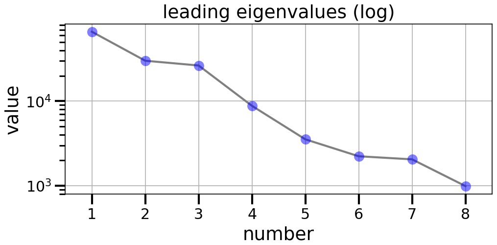
Figure 7Leading eigenvalues of biogenic emissions for independent sensitivities including additional uncertainties. Plotting conventions are the same as in Fig. 5.
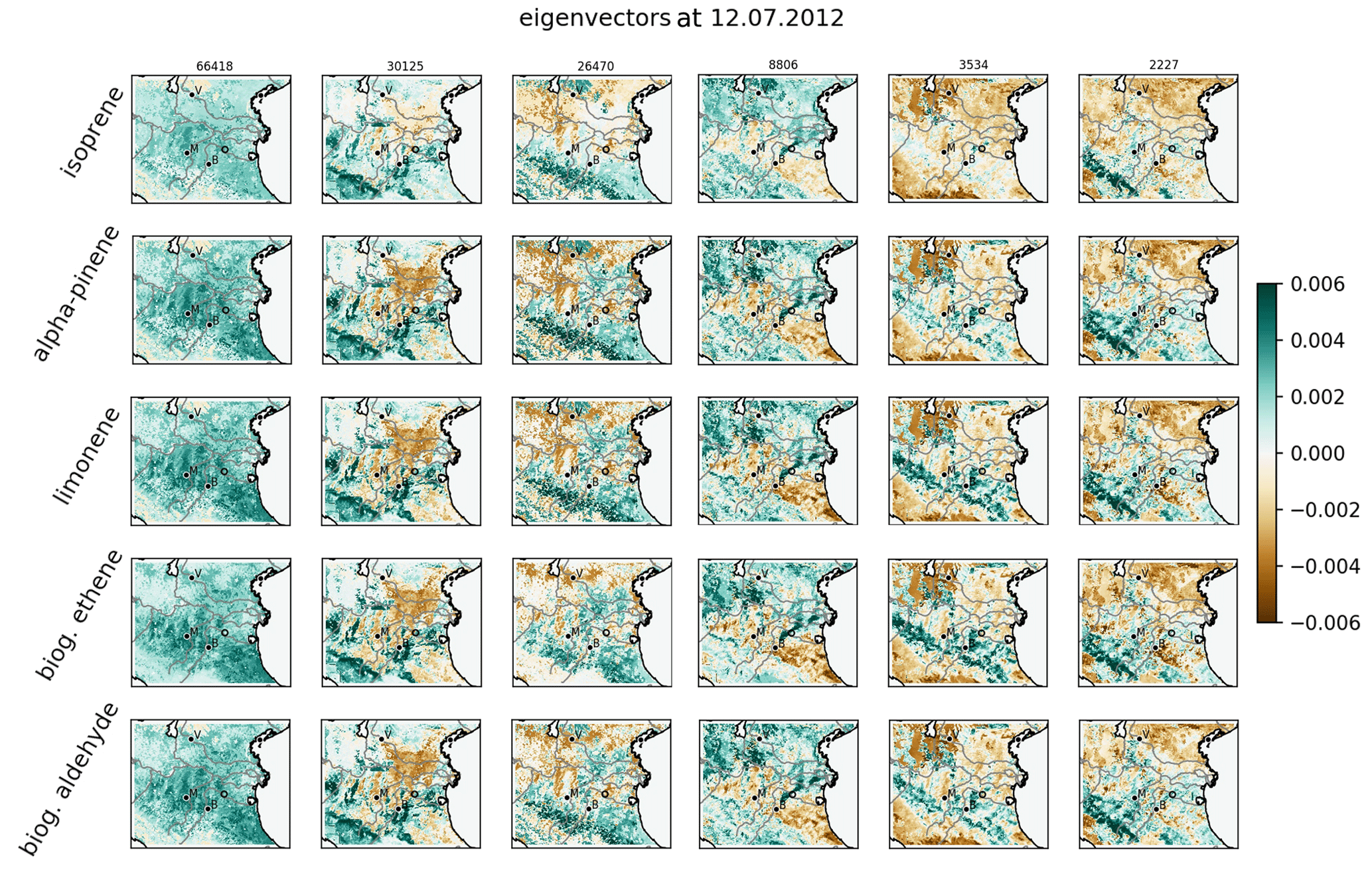
Figure 8Leading eigenvectors for independent sensitivities including additional uncertainties. Plotting conventions are the same as in as in Fig. 6.
As for combined sensitivities, the eigenmode decomposition extracts perpendicular components from the set of independent sensitivities. The eigenvalues shown in Fig. 7 state a similar decrease of eigenvalues for independent sensitivities compared to the combined method. Highly similar sizes and decrease rates of the leading eigenvalues indicate a reasonable representation of the leading uncertainties by the independent method. However, nonlinearities arising from combined changes in the land surface model with global meteorology or boundary layer schemes are not captured by the linear assumption of independent sensitivities.
According to the corresponding eigenvectors in Fig. 8, the first eigenmode represents common features of the a priori uncertainty and the other independent sensitivities. While the second eigenmode is closely related to the effects of drought response and the land surface model, the sensitivity to land use dominates the third eigenmode. Aside from this, highly similar signals in eigenvectors for different biogenic gases state a considerably large correlation between them. Nevertheless, individual patterns of each biogenic gas are also represented by the leading eigenmodes for independent sensitivities. These patterns are also found for the eigenvectors of combined sensitivities (compare Fig. 6), which confirms the suitability of the independent method with respect to multiple parameters. Note that the consideration of additional uncertainties in the independent method does not allow for a direct comparison of individual eigenmodes.
4.5 Ensemble generation
The different setups of the covariances from combined and independent sensitivities prohibit a direct comparison of their perturbations. As the ensemble generation from leading eigenmodes does not differ between these two setups (compare Sect. 3.3), resulting perturbations are only shown for independent sensitivities.
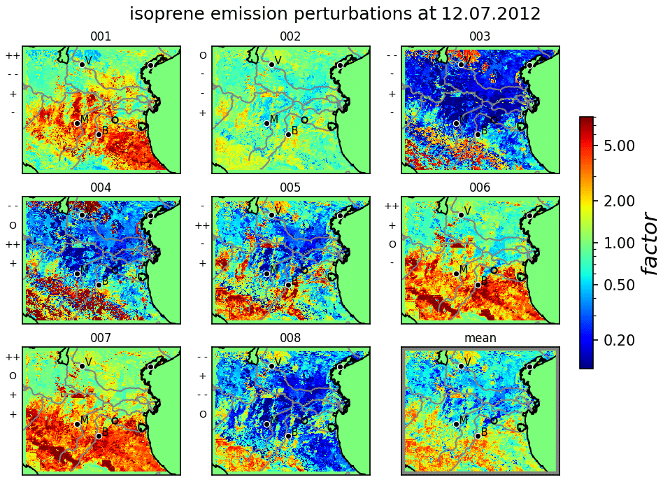
Figure 9Perturbations of isoprene emissions for independent sensitivities, including additional uncertainties given as factors w.r.t reference emissions. Random realizations of stochastic coefficients for the leading eigenmodes of each member are indicated left of each subplot: + +, large positive value (); +, small positive value (); O, very small absolute value (); −, small negative value (); − −: large negative value ()). The lower-right subplot gives the ensemble mean factors. Some major cities (Verona, Bologna, Modena) are indicated by their initial letters.
Figure 9 displays eight realizations of perturbations in terms of emission factors for isoprene for independent sensitivities. The perturbation factors of all biogenic emissions are calculated by multiplying the independent mean factors of the sensitivities with different realizations of the KL expansion. As the KL expansion does not affect the mean values, ensemble mean emission factors remain similar to the one of the sensitivities (compare Fig. 4). Although differences in perturbation factors are large, this suggests a reasonable sampling of the eight realizations. Concerning the individual members, the high number of significant uncertainties results in emission factors ranging up to more than 1 order of magnitude. Each realization is influenced by different combinations of the leading eigenmodes resulting in different perturbation patterns. While realization 001, 006, and 007 are dominated by a positive contribution of the first eigenmode, the effect of the second mode is clearly visible when comparing realization 001 and 006. Comparing realization 004 and 008, the most significant differences are induced by the third eigenmode. Due to the fast decrease of eigenmodes, comparably small contributions of the remaining modes remain invisible in the perturbation factors. Thus, the comprised KL ensemble is restricted to dominant uncertainties indicated by the leading eigenmodes. In this case, these uncertainties are mainly induced by sensitivities to various surface conditions, which is in accordance with Vogel and Elbern (2021a).
4.6 Ensemble evaluation
The performance of the KL ensemble perturbations is evaluated by ensemble statistics. Note that this evaluation only relates to the algorithm itself, i.e., how well the algorithm is able to capture the uncertainties indicated by the sensitivities. The question of how well the sensitivities represent the true parameter uncertainties is not part of the evaluation and beyond the scope of this study. In order to be able to compare the statistics of the KL ensembles using combined and independent sensitivities, I=6 model arguments are considered for both setups. While the setup of 32 combined sensitivities is the same as in the previous sections (Jcombi=32), no additional uncertainties were included in the independent setup (Jindep=7). Despite this, the setup remains as described in Sect. 4.2.
In Fig. 10, statistics of the ensemble perturbation factors from the KL algorithm with combined sensitivities are compared to statistics of the sensitivity factors from 32 combined sensitivities. Because these 32 combined sensitivities serve as input for the algorithm in the combined method, the ensemble statistics at all locations should ideally coincide with the identity line. Thus, deviations from the identity line give an indication of the sampling error induced by the limited number of used eigenmodes and the low number of eight realizations compared to the dimension of the problem. Mean isoprene emission factors for the combined method are well represented by the KL algorithm: deviations remain below 20 % for almost all locations (Fig. 10a).
Ensemble standard deviations show more significant deviations (Fig. 10b). For low and medium values, standard deviations of the KL ensemble with combined sensitivities range from 75 % until 130 % of the respective input values. This almost homogeneous scatter around the input values is likely induced by minor uncertainties that are not captured by the leading eigenmodes. At some locations, the KL ensemble produces a set of high standard deviations between 5.0 and 8.0 that are not found in the sensitivities. While the standard deviation is overestimated at these locations, the ensemble mean at these locations is slightly underestimated (sensitivities approx. 3.0, combined ensemble perturbations approx. 2.0; see Fig. 10a).
These deviations can be related to the low ensemble size and are expected to reduce for larger ensemble sizes. Additionally, limiting sensitivity factors in the KL algorithm may also affect sensitivity statistics in this case (compare Sect. 4.2).
The independent method induces larger deviations of mean isoprene emission factors from the mean combined sensitivities. The increase in deviations mainly represent the additional inaccuracy due to the assumption of independent sensitivities. Note that the 32 combined sensitivities used in the evaluation are a subset of 64 possible combinations (compare Sect. 4.2). Because the independent method approximates all combinations of sensitivities, some deviations might also relate to the selection of the 32 combined sensitivities. Ensemble mean factors correlate well with the combined sensitivities and deviations remain between −25 % and +50 % for most locations (Fig. 10a). While only 7 instead of 32 – or ideally 64 – sensitivities are required for this setup, the spread of mean factors is about twice the spread for the combined ensemble setup. Deviations of ensemble standard deviations are also slightly increased for the independent method (Fig. 10b). The overestimation of high standard deviations produced by the combined method is reduced in the independent method. At some locations, standard deviations of about 2.0 in the combined sensitivities are underestimated by the KL ensemble with independent sensitives (standard deviations approx. 1.5). These differences are likely due to nonlinear effects from combining sensitivities that are neglected in this setup. Nevertheless, the ensemble standard deviations at most locations are well represented by the KL ensemble with independent sensitivities.
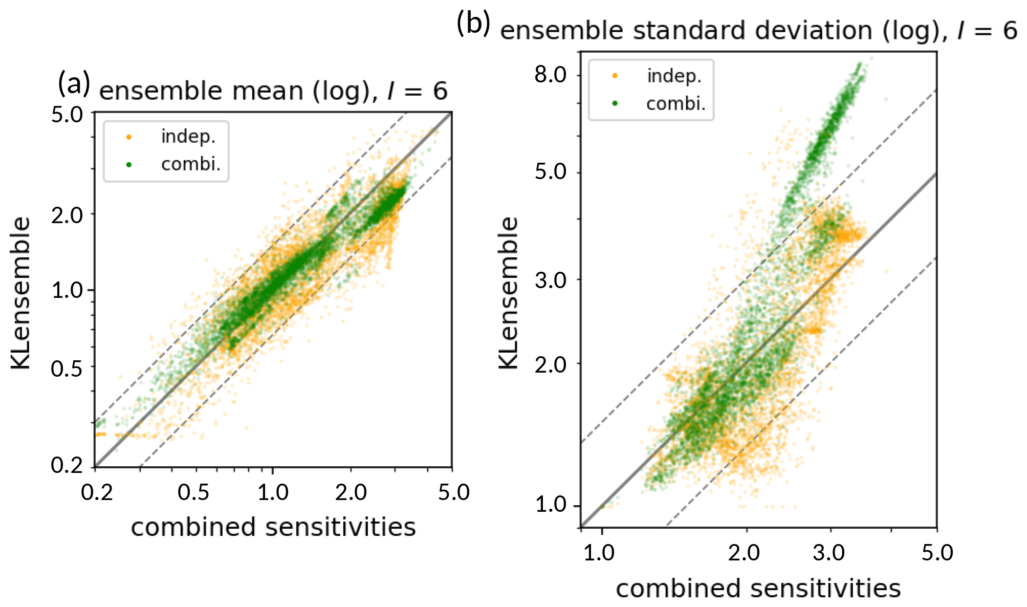
Figure 10Scatterplot of ensemble statistics for isoprene emission perturbations. Shown are logarithmic ensemble mean (a) and standard deviations (b) of the KL ensemble perturbations at each grid box as function of combined sensitivities. Ensemble statistics are shown for 32 combined (green) and 7 independent (orange) sensitivities, which both refer to the same set of I=6 considered arguments. The solid gray line indicates the identity line (e.g., for the ensemble mean) to the set of 32 combined sensitivities; the dashed gray lines represent an overestimation or underestimation by a factor of 1.5 (e.g., and ).
This section provides a discussion of different aspects regarding the potential and limitations of the KL ensemble generation approach. Concerning the formulation of the algorithm, ensemble perturbations are created from covariances of the stochastic process. The use of the KL expansion ensures that for large ensemble sizes the statistics of the perturbations converge towards their input values determined by the covariances. Consequently, the accuracy of the KL ensemble in representing the true uncertainties crucially relies on the formulation of the covariances. Uncertainties not considered in the formulation of the covariances cannot be captured by the KL ensemble. The major benefit of the approach lies in the optimal properties of the perturbations focusing on leading uncertainties, providing an optimal coverage of uncertainties even for low ensemble sizes. Although the greatest benefit is achieved for highly correlated parameters, the algorithm is assumed to efficiently combine the major uncertainties even for uncorrelated parameters. In case of missing correlations and therefore a lack of ensemble reduction potential, the KL approach retains more leading eigenmodes and does not suppress required degrees of freedom.
By extracting leading eigenmodes from parameter covariances, the problem is transferred to a low-dimensional subspace spanned by the set of leading eigenmodes. This makes the approach highly efficient in covering dominant uncertainties compared to random perturbations at each location. For this uncondensed random approach, perturbations would be sampled from the complete N-dimensional space given by all considered model parameters at all grid boxes. Compared to the uncondensed approach, the sampling space from which the KL perturbations are sampled is reduced to a D-dimensional eigenmode subspace. The higher the parameter correlations, the less eigenmodes need to be considered in order to obtain sufficient sampling of uncertainties. Most atmospheric chemical parameters have high spatial and cross-parameter correlations, which enable D≪N and thus significant reduction of the sampling space. In the results presented in this study, this has been demonstrated for a set of biogenic emissions with dimension 2×10⁶. In this case, sampling about 10 ensemble members from the leading eigenmodes is sufficient to cover the leading uncertainties of the high-dimensional parameters. The required numbers of eigenmodes and ensemble perturbations depend on the desired level of detail of the ensemble. Independent of the level of detail, the KL expansions ensure an optimal estimation of covariances by the calculated perturbations.
Table 2Computation time for the solution of the eigenproblem in the KL ensemble generation algorithm for representative setups. The dimension of the system was reduced as described in Sect. 4. The relative computing time is given w.r.t. 8 eigenmodes from 32 combined sensitivities of 5 parameters (*). The last two lines show the setups of independent (indep) and combined (combi) sensitivities presented in this study, respectively.
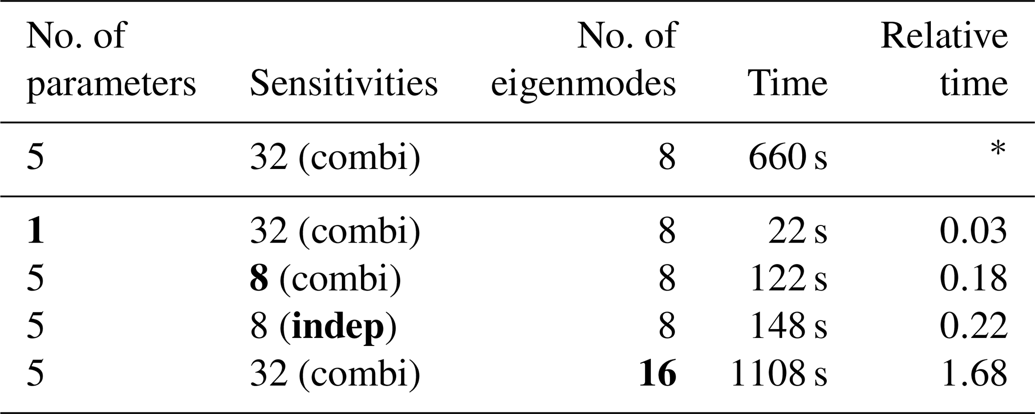
No. of parameters is the number of different model parameters considered, sensitivities is number and type of sensitivities used for covariance construction, no. of eigenmodes is the number of eigenvalues and vectors calculated, time is the physical time required for computation of perturbations, and relative time is the computation time divided by reference computation time.
Once the sensitivities are calculated, the computational effort required for the generation of Karhunen–Loéve (KL) perturbations is mainly consumed by the numerical solution of the eigenproblem. The highly efficient parallelization of the solution of the eigenproblem by P-ARPACK renders the algorithm suitable for high-dimensional systems. Table 2 summarizes the computation time and relevant properties for selected setups. By definition, the computing time is proportional to the size of the covariance matrix, which increases quadratically with the dimension of the considered model parameters. Note that the computing time is given as wall clock time for calculating the perturbations. Due to the parallelization of the computation, the total CPU time scales linearly with the number of cores used. Independent of the number of cores, the computational effort for calculating perturbations is low compared to running a model simulation. Despite small variations, the computing time increases linearly with the number of eigenmodes calculated. The required computational effort appears to increase approximately linearly with the number of sensitivities for covariance construction and the number of calculated eigenmodes. In this case, doubling the number of considered sensitivities increases the computing time by about a factor of 2.3. Applying the assumption of independent sensitivities reduces the number of used sensitivities in this study from 32 combined to 8 independent sensitivities including additional uncertainties. In addition to the strong reduction of computation time for simulating the sensitivities, the time for solving the eigenproblem reduces by about a factor of 4.5.
The results presented in this study demonstrate a considerable reduction of required computational resources under the assumption of independent sensitivities. As this method assumes linearity of parameter sensitivities, it may not be a sufficient approximation for all atmospheric parameters. However, the linear assumption relates to sensitivities of the perturbed parameters to model configurations. In other words, nonlinear effects resulting from the combination of different model arguments are disregarded. Note that this does not affect the impact of the parameters on prognostic fields like trace gas distributions and their propagation in time, which is beyond the ensemble generation and may still be highly nonlinear. Thus, the presented approach may also be suitable to be applied to parameters in NWP with highly nonlinear model dynamics. The sufficiency of this approximation for a model parameter in relation to the reduction of computational efforts needs to be evaluated for each specific application setup.
The developed KL approach may extended to inverse optimization of model parameters. The generated parameter ensemble can be used to estimate state-dependent model covariances in an ensemble data assimilation system. If requested by the type of data assimilation algorithm, inverse square roots of covariance matrices are readily available for preconditioned minimization. Furthermore, the KL expansion of the parameter fields enables an advanced optimization approach. Instead of optimizing the parameter fields in its full N-dimensional space, the optimization can be performed in the reduced subspace spanned by the D leading eigenmodes. As the leading eigenmodes represent the dominant uncertainties of the parameters, the optimization would be restricted to those. In this case, the set of stochastic coefficients would be replaced by the optimization variable (compare Eq. 15), which is fully determined by as low as D observations. Thus, this approach may be able to provide a rough, yet efficient optimization of model parameter fields with a low number of observations. For both optimization approaches, spurious correlations resulting from the restriction to leading uncertainties must be addressed by location measures.
This study introduces an optimized ensemble generation approach in which model parameters are efficiently perturbed according to their correlations. The approach is based on the fact that the forecast model acts as a dynamical system with its specific spatial and multivariate couplings of the atmospheric state. It applies the Karhunen–Loéve expansion, which approximates covariances of the model parameters by a limited set of leading eigenmodes. These modes represent the coupled leading uncertainties from which perturbations can be sampled efficiently. Based on this, stochastic sampling for ensemble generation is performed in an uncorrelated subspace spanned by the eigenmodes. Generally, the presented algorithm is applicable to any set of model parameters in high-dimensional atmospheric systems, as long as their joint uncertainties remain in the linear regime. Through the reduction of the sampling space, it is shown that the stochastic dimension of the problem can be reduced significantly. This makes the algorithm suitable for efficient ensemble generation of high-dimensional atmospheric models, where the computational costs are a critical and limiting quantity.
Focusing on model parameters that depend on local environmental conditions, state-dependent covariances are approximated from various related sensitivities. Generally, the covariances required for this approach can be defined in any way which is suitable to reflect the uncertainty of our knowledge. Covariance construction based on parameter sensitivities as presented in this study is just one among many. Potential deficiencies in the construction could be identified from a posteriori evaluation of the full ensemble. This would allow for an ongoing adjustment of the algorithm depending on the specific application.
As simulations of all possible combinations of sensitivities are computationally demanding, independent sensitivities are introduced in this study. Assuming tangent linearity, multiple combined sensitivities can be represented by a low number of independent sensitivities. Representative results indicate that the major properties of leading sensitivities are captured by independent sensitivities. Considering 2 realizations of 6 model arguments, only 7 independent sensitivities out of a total number of 64 combined sensitivities are required. Thus, the method of independent sensitivities reduces the computational effort of model simulations prior to ensemble generation tremendously. Besides the reduction of computational resources, this method allows for the integration of different kinds of uncertainties in a convenient way. However, in many cases the assumption of independent sensitivities may not be a good approximation. The user has to decide if the computational benefit justifies the neglection of nonlinear effects.
The potential of the KL ensemble generation approach is investigated for regional forecasts of a set of biogenic emissions. During the selected case study in the Po valley in July 2012, biogenic emissions were exceptionally sensitive to several land surface properties. In this case, the eigenmode decomposition indicates high correlations of uncertainties in the regional domain as well as between different biogenic gases. Rapidly decreasing eigenvalues state the dominant contributions of only a few orthogonal components from a global point of view. Resulting perturbation factors for isoprene emissions created by the KL ensemble generation algorithm range between less than 0.1 up to 10. Although some realizations show common perturbation patterns, significant contributions from the subsequent eigenmodes can clearly be identified from the eight realizations. This indicates that the KL ensemble generation approach is able to sufficiently sample the subspace of leading uncertainties using as few as 10 members in this case. Moreover, as each eigenmode represents common patterns of different sensitivities, the realizations are affected by the whole set of underlying sensitivities.
A comprehensive evaluation of KL ensemble perturbations would be based on a representative amount of observational data. Comparing to observed trace gas concentrations requires the consideration of uncertainties related to different processes affecting those concentrations, which is out of the scope of this study. Instead, the performance of the KL algorithm itself was evaluated using ensemble statistics. The statistical comparison of the KL perturbations with the sensitivities used as input states sufficient representation of the main aspects. Both combined and independent methods were able to capture the main uncertainties, while smaller contributions were neglected according to the objective of the algorithm.
The presented application of the KL ensemble generation approach demonstrates its potential for an efficient estimation of forecast uncertainties induced by model parameters in high-dimensional atmospheric models. Specifically, the presented algorithm allows for (1) an efficient estimation of various sensitivities based on the assumption of independent sensitivities, (2) an efficient extraction of leading coupled uncertainties using highly parallelized eigenmode decomposition, and (3) an efficient generation of perturbations of high-dimensional parameter fields by the Karhunen–Loéve expansion. This motivates its promising application to various state-dependent parameters in chemistry transport modeling and potentially also in other atmospheric models. A follow-up study will investigate and validate probabilistic forecasts of biogenic gases with respect to different state-dependent model parameters during the PEGASOS campaign in the Po valley in 2012. Furthermore, the approach may also be applied to other kinds of model parameters, where sufficient covariances need to be estimated accordingly. In this context, the reduction to leading coupled uncertainties offers the ability to account for dominant uncertainties across all parameters influencing atmospheric chemical forecasts. This would provide a significant step in the transition from deterministic to probabilistic chemistry transport modeling.
Given a set of independent sensitivities with implementation of each model argument at position s ∈ S. Assuming independence of sensitivities, each combined sensitivity is given by
where the total number of combined sensitivities is
The mean value μ(s) of all combined sensitivities at position s ∈ S can be calculated from the set of independent sensitivities as follows.
The covariance of all combined sensitivities at positions can be calculated from the sets of independent sensitivities as follows.
Table B1Overview of model setups used as combined sensitivities. A detailed description of the abbreviations and model implementations has been provided by Vogel and Elbern (2021a). The reference setup is denoted as *, and deviations from this reference are written in bold letters (PX is the Pleim–Xiu surface layer parameterization; Du is the Dudhia shortwave radiation parameterization).

The code of the KL ensemble generation algorithm available at https://doi.org/10.5281/zenodo.4468571 (Vogel and Elbern, 2021b) contains the routines that are important for generating the results presented in this study. The data used as input for the production of the results and the output of the algorithm are available at https://doi.org/10.5281/zenodo.4772909 (Vogel and Elbern, 2021c).
AV developed and implemented the algorithm, performed the simulations, and wrote the manuscript. HE provided the basic idea, supervised the work, contributed to the developments, and helped in the preparation of the manuscript.
The authors declare that they have no competing interests.
Publisher’s note: Copernicus Publications remains neutral with regard to jurisdictional claims in published maps and institutional affiliations.
This work has been funded by the Helmholtz Climate Initiative REKLIM (Regional Climate Change), a joint research project of the Helmholtz Association of German research centers (HGF) under grant no. REKLIM-2009-07-16. The authors gratefully acknowledge the computing time granted through JARA-HPC on the supercomputer JURECA (Jülich Supercomputing Centre, 2018) at Forschungszentrum Jülich. The authors thank the Institute of Geophysics and Meteorology at the University of Cologne for the opportunity to finish the work presented here. The authors thank the two anonymous reviewers for their valuable suggestions.
The article processing charges for this open-access publication were covered by the Forschungszentrum Jülich.
This paper was edited by Andrea Stenke and reviewed by two anonymous referees.
Auger, L. and Tangborn, A.: A wavelet-based reduced rank Kalman filter for assimilation of stratospheric chemical tracer observations, Mon. Weather Rev., 132, 1220–1237, https://doi.org/10.1175/1520-0493(2004)132<1220:AWRRKF>2.0.CO;2, 2004. a
Bauer, P., Thorpe, A., and Brunet, G.: The quiet revolution of numerical weather prediction, Nature, 525, 47–55, https://doi.org/10.1038/nature14956, 2015. a
Bocquet, M., Elbern, H., Eskes, H., Hirtl, M., Žabkar, R., Carmichael, G. R., Flemming, J., Inness, A., Pagowski, M., Pérez Camaño, J. L., Saide, P. E., San Jose, R., Sofiev, M., Vira, J., Baklanov, A., Carnevale, C., Grell, G., and Seigneur, C.: Data assimilation in atmospheric chemistry models: current status and future prospects for coupled chemistry meteorology models, Atmos. Chem. Phys., 15, 5325–5358, https://doi.org/10.5194/acp-15-5325-2015, 2015. a
Boynard, A., Beekmann, M., Foret, G., Ung, A., Szopa, S., Schmechtig, C., and Coman, A.: An ensemble assessment of regional ozone model uncertainty with an explicit error representation, Atmos. Environ., 45, 784–793, https://doi.org/10.1016/j.atmosenv.2010.08.006, 2011. a
Buizza, R.: Introduction to the special issue on “25 years of ensemble forecasting”, Q. J. Roy. Meteor. Soc., 145, 1–11, https://doi.org/10.1002/qj.3370, 2019. a
Buizza, R., Tribbia, J., Molteni, F., and Palmer, T.: Computation of optimal unstable structures for a numerical weather prediction model, Tellus A, 45, 388–407, https://doi.org/10.1034/j.1600-0870.1993.t01-4-00005.x, 1993. a
Buizza, R., Milleer, M., and Palmer, T. N.: Stochastic representation of model uncertainties in the ECMWF ensemble prediction system, Q. J. Roy. Meteor. Soc., 125, 2887–2908, https://doi.org/10.1002/qj.49712556006, 1999. a
Candiani, G., Carnevale, C., Finzi, G., Pisoni, E., and Volta, M.: A comparison of reanalysis techniques: Applying optimal interpolation and Ensemble Kalman Filtering to improve air quality monitoring at mesoscale, Sci. Total Environ., 458-460, 7–14, https://doi.org/10.1016/j.scitotenv.2013.03.089, 2013. a
Cohn, S. E. and Todling, R.: Approximate Data Assimilation Schemes for Stable and Unstable Dynamics, J. Met. Soc. Jpn., 74, 63–75, 1996. a
Elbern, H., Strunk, A., Schmidt, H., and Talagrand, O.: Emission rate and chemical state estimation by 4-dimensional variational inversion, Atmos. Chem. Phys., 7, 3749–3769, https://doi.org/10.5194/acp-7-3749-2007, 2007. a, b, c, d
Emili, E., Gürol, S., and Cariolle, D.: Accounting for model error in air quality forecasts: an application of 4DEnVar to the assimilation of atmospheric composition using QG-Chem 1.0, Geosci. Model Dev., 9, 3933–3959, https://doi.org/10.5194/gmd-9-3933-2016, 2016. a, b
Galin, M. B.: Study of the Low-Frequency Variability of the Atmospheric General Circulation with the Use of Time-Dependent Empirical Orthogonal Functions, Atmos. Ocean. Phys., 43, 15–23, https://doi.org/10.1134/S0001433807010021, 2007. a
Gaubert, B., Coman, A., Foret, G., Meleux, F., Ung, A., Rouil, L., Ionescu, A., Candau, Y., and Beekmann, M.: Regional scale ozone data assimilation using an ensemble Kalman filter and the CHIMERE chemical transport model, Geosci. Model Dev., 7, 283–302, https://doi.org/10.5194/gmd-7-283-2014, 2014. a
Geiger, H., Barnes, I., Bejan, I., Benter, T., and Spittler, M.: The tropospheric degradation of isoprene: An updated module for the regional atmospheric chemistry mechanism, Atmos. Environ., 37, 1503–1519, https://doi.org/10.1016/S1352-2310(02)01047-6, 2003. a
Goris, N. and Elbern, H.: Singular vector-based targeted observations of chemical constituents: description and first application of the EURAD-IM-SVA v1.0, Geosci. Model Dev., 8, 3929–3945, https://doi.org/10.5194/gmd-8-3929-2015, 2015. a
Guenther, A. B., Jiang, X., Heald, C. L., Sakulyanontvittaya, T., Duhl, T., Emmons, L. K., and Wang, X.: The Model of Emissions of Gases and Aerosols from Nature version 2.1 (MEGAN2.1): an extended and updated framework for modeling biogenic emissions, Geosci. Model Dev., 5, 1471–1492, https://doi.org/10.5194/gmd-5-1471-2012, 2012. a, b, c
Guilloteau, C., Mamalakis, A., Vulis, L., Le, P. V. V., Georgiou, T. T., and Foufoula-Georgiou, E.: Rotated Spectral Principal Component Analysis (rsPCA) for Identifying Dynamical Modes of Variability in Climate Systems, J. Cimate, 34, 715–736, https://doi.org/10.1175/JCLI-D-20-0266.1, 2021. a
Hanea, R., Velders, G., and Heemink, A.: Data assimilation of ground-level ozone in Europe with a Kalman filter and chemistry transport model, J. Geophys. Res.-Atmos., 109, D10302, https://doi.org/10.1029/2003JD004283, 2004. a
Hanea, R. G. and Velders, G. J. M.: A hybrid Kalman filter algorithm for large-scale atmospheric chemistry data assimilation, Mon. Weather Rev., 135, 140–151, https://doi.org/10.1175/MWR3269.1, 2007. a
Hanna, S. R., Chang, J. C., and Fernau, M. E.: Monte carlo estimates of uncertainties in predictions by a photochemical grid model (UAM-IV) due to uncertainties in input variables, Atmos. Environ., 32, 3619–3628, https://doi.org/10.1016/S1352-2310(97)00419-6, 1998. a, b
Hannachi, A., Jolliffe, I. T., and Stephenson, D. B.: Empirical orthogonal functions and related techniques in atmospheric science: A review, Int. J. Climatol., 27, 1119–1152, https://doi.org/10.1002/joc.1499, 2007. a
Houtekamer, P. L., Lefaivre, L., Derome, J., Ritchie, H., and Mitchell, H. L.: A System Simulation Approach to Ensemble Prediction, Mon. Weather Rev., 124, 1225–1242, https://doi.org/10.1175/1520-0493(1996)124<1225:ASSATE>2.0.CO;2, 1996. a, b
Jülich Supercomputing Centre: JURECA: Modular supercomputer at Jülich Supercomputing Centre, J. Large-scale Res. Fac., 4, A132, https://doi.org/10.17815/jlsrf-4-121-1, 2018. a
Karhunen, K.: Über lineare methoden in der Wahrscheinlichkeitsrechnung, Annales Academiae Scientarum Fennicae, 37, 3–79, 1947. a
Lehoucq, R. B., Sorensen, D. C., and Yang, C.: ARPACK Users Guide: Solution of Large Scale Eigenvalue Problems by Implicitly Restarted Arnoldi Methods, available at: https://www.caam.rice.edu/software/ARPACK/UG/ug.html (last access: 9 August 2021), 1997. a, b
Leutbecher, M.: Ensemble size: How suboptimal is less than infinity?, Q. J. Roy. Meteor. Soc., 145, 107–128, https://doi.org/10.1002/qj.3387, 2019. a
Leutbecher, M., Lock, S.-J., Ollinaho, P., Lang, S. T. K., Balsamo, G., Bechtold, P., Bonavita, M., Christensen, H. M., Diamantakis, M., Dutra, E., English, S., Fisher, M., Forbes, R. M., Goddard, J., Haiden, T., Hogan, R. J., Juricke, S., Lawrence, H., MacLeod, D., Magnusson, L., Malardel, S., Massart, S., Sandu, I., Smolarkiewicz, P. K., Subramanian, A., Vitart, F., Wedi, N., and Weisheimer, A.: Stochastic representations of model uncertainties at ECMWF: state of the art and future vision, Q. J. Roy. Meteor. Soc., 143, 2315–2339, https://doi.org/10.1002/qj.3094, 2017. a
Liu, Y., Wang, L., Zhou, W., and Chen, W.: Three Eurasian teleconnection patterns: spatial structures, temporal variability, and associated winter climate anomalies, Clim. Dynam., 42, 2817–2839, https://doi.org/10.1007/s00382-014-2163-z, 2014. a
Lock, S.-J., Lang, S. T. K., Leutbecher, M., Hogan, R. J., and Vitart, F.: Treatment of model uncertainty from radiation by the Stochastically Perturbed Parametrization Tendencies (SPPT) scheme and associated revisions in the ECMWF ensembles, Q. J. Roy. Meteor. Soc., 145, 75–89, https://doi.org/10.1002/qj.3570, 2019. a
Loéve, M.: Fonctions aleatoires du second ordre, Processus Stochastiques et Mouvement Brownien, Gauthier-Villars, Paris, 42th edn., 1948. a
McKeen, S., Chung, S. H., Wilczak, J., Grell, G., Djalalova, I., Peckham, S., Gong, W., Bouchet, V., Moffet, R., Tang, Y., Carmichael, G. R., Mathur, R., and Yu, S.: Evaluation of several PM2.5 forecast models using data collected during the ICARTT/NEAQS 2004 field study, J. Geophys. Res.-Atmos., 112, D10S20, https://doi.org/10.1029/2006JD007608, 2007. a
Pöschl, U., Kuhlmann, R., Poisson, N., and Crutzen, P.: Development and Intercomparison of Condensed Isoprene Oxidation Mechanisms for Global Atmospheric Modeling, J. Atmos. Chem., 37, 29–52, https://doi.org/10.1023/A:1006391009798, 2000. a
Schutgens, N. A. J., Miyoshi, T., Takemura, T., and Nakajima, T.: Applying an ensemble Kalman filter to the assimilation of AERONET observations in a global aerosol transport model, Atmos. Chem. Phys., 10, 2561–2576, https://doi.org/10.5194/acp-10-2561-2010, 2010. a
Schwab, C. and Todor, R. A.: Karhunen-Loève Approximation of Random Fields by Generalized Fast Multipole Methods, J. Comput. Phys., 217, 100–122, https://doi.org/10.1016/j.jcp.2006.01.048, 2006. a, b
Shutts, G.: A kinetic energy backscatter algorithm for use in ensemble prediction systems, Q. J. Roy. Meteor. Soc., 131, 3079–3102, https://doi.org/10.1256/qj.04.106, 2005. a
Siripatana, A., Mayo, T., Knio, O., Dawson, C., Le Maitre, O., and Hoteit, I.: Ensemble Kalman filter inference of spatially-varying Manning's n coefficients in the coastal ocean, J. Hydrol., 562, 664–684, https://doi.org/10.1016/j.jhydrol.2018.05.021, 2018. a
Skamarock, W. C., Klemp, J. B., Dudhia, J., Gill, D. O., Barker, D. M., Duda, M. G., Huang, X.-Y., Wang, W., and Powers, J. G.: A Description of the Advanced Research WRF Version 3, National Center for Atmospheric Research Boulder, Colorado, USA, NCAR technical note, 2008. a
Sorensen, D.: Implicitly Restarted Arnoldi/Lanczos Methods for Large Scale Eigenvalue Calculations, in: Parallel Numerical Algorithms, ICASE/LaRC Interdisciplinary Series in Science and Engineering, edited by: Keyes, D., Sameh, A., and Venkatakrishnan, V., vol 4., Springer, Dordrecht, 1997. a
Toth, Z. and Kalnay, E.: Ensemble forecasting at NMC: The generation of perturbations, B. Am. Meteorol. Soc., 74, 2317–2330, 1993. a
Vautard, R., Blond, N., Schmidt, H., Derognat, C., and Beekmann, M.: Multi-model ensemble ozone forecasts over Europe: analysis of uncertainty, Mesoscale Transport of Air Pollution, OA15. EGS XXXVI General Assembly, Nice, France, European Geophysical Society, 25–30 March 2001, 26 pp., 2001. a
Verlaan, M. and Heemink, A. M.: Data assimilation schmes for non-linear shallow water flow models, Adv. Fluid Mech., 96, 277–286, 1996. a
Vogel, A. and Elbern, H.: Identifying forecast uncertainties for biogenic gases in the Po Valley related to model configuration in EURAD-IM during PEGASOS 2012, Atmos. Chem. Phys., 21, 4039–4057, https://doi.org/10.5194/acp-21-4039-2021, 2021a. a, b, c, d, e, f, g, h, i, j
Vogel, A. and Elbern, H.: Karhunen-Loéve (KL) Ensemble Routines of the EURAD-IM modeling system, Zenodo, https://doi.org/10.5281/zenodo.4468571, 2021b. a
Vogel, A. and Elbern, H.: Data of Karhunen-Loéve (KL) ensemble generation algorithm for biogenic emissions from EURAD-IM, Zenodo, https://doi.org/10.5281/zenodo.4772909, 2021c. a
Xian, P., Reid, J. S., Hyer, E. J., Sampson, C. R., Rubin, J. I., Ades, M., Asencio, N., Basart, S., Benedetti, A., Bhattacharjee, P. S., Brooks, M. E., Colarco, P. R., da Silva, A. M., Eck, T. F., Guth, J., Jorba, O., Kouznetsov, R., Kipling, Z., Sofiev, M., Perez Garcia-Pando, C., Pradhan, Y., Tanaka, T., Wang, J., Westphal, D. L., Yumimoto, K., and Zhang, J.: Current state of the global operational aerosol multi-model ensemble: An update from the International Cooperative for Aerosol Prediction (ICAP), Q. J. Roy. Meteor. Soc., 145, 176–209, https://doi.org/10.1002/qj.3497, 2019. a
Xiu, D.: Numerical Methods for Stochastic Computations: A Spectral Method Approach, Princeton University Press, Princeton, NJ, USA, 2010. a
Zhang, Y., Bocquet, M., Mallet, V., Seigneur, C., and Baklanov, A.: Real-time air quality forecasting, part I: History, techniques, and current status, Atmos. Environ., 60, 632 – 655, https://doi.org/10.1016/j.atmosenv.2012.06.031, 2012a. a
Zhang, Y., Bocquet, M., Mallet, V., Seigneur, C., and Baklanov, A.: Real-time air quality forecasting, part II: State of the science, current research needs, and future prospects, Atmos. Environ., 60, 656–676, https://doi.org/10.1016/j.atmosenv.2012.02.041, 2012b. a
- Abstract
- Introduction
- Concept of sensitivity estimation
- Algorithm
- Application to biogenic emissions
- Discussion
- Conclusions
- Appendix A: Derivation of independent mean and covariance
- Appendix B: Setup of combined sensitivities
- Code and data availability
- Author contributions
- Competing interests
- Disclaimer
- Acknowledgements
- Financial support
- Review statement
- References