Multi-sensor analyses of the skin temperature for the assimilation of satellite radiances in the European Centre for Medium-Range Weather Forecasts (ECMWF) Integrated Forecasting System (IFS, cycle 47R1)

The assimilation of clear-sky radiance in the European Centre for Medium-Range Weather Forecasts (ECMWF) atmospheric analysis relies on the clear-sky radiances observation operator. Some of these radiances have frequencies that make them sensitive to both the surface and atmosphere. Because the atmospheric and surface analyses are currently not strongly coupled, a specific treatment of the surface is required. The observation operator specifically expects a skin temperature value at the observation location and time as well as the profiles of the atmospheric variables along the viewing path. This skin temperature is added to the control variable and optimised simultaneously with all of the atmospheric variables to produce optimal simulated radiances.

We present two approaches to add the skin temperature to the control variable. In the current TOVS Control Variable (TOVSCV) approach, a series of skin temperature values per observation location is added to the control variable. Effectively, in the optimisation process, the skin temperature acts as a sink variable in observation space and is uncoupled from the skin temperature at other locations. In the novel SKin Temperature in the Extended Control Vector (SKTECV) approach, two-dimensional skin temperature fields are added to the control variable. All clear-sky radiances then participate in the optimisation of these two-dimensional fields, and the analysis produces temporally and spatially consistent skin temperature fields.

We compare the two approaches over two seasons of 3 months each. Overall, there is a neutral impact of the new approach on the analysis and forecast. Moreover, there is some evidence that the contribution of the subsurface layers should be represented in the new approach for the skin temperature associated with the microwave instruments.

1 Introduction

Data assimilation methods used in numerical weather prediction (NWP) exploit all of the available observations by computing the difference between them and the model state at the observation time and location. The latter is obtained by first integrating the model state in time and then transforming it into an observation equivalent using the so-called observation operator. The observation operator is dependent on the observation type. For most of the in situ observations, the observation operator is a simple time and space interpolation. For other observation types, the operator can be much more complex. For instance, a fast and accurate radiative transfer model to simulate observations is required for satellite observations. Furthermore, the complexity of the observation operator increases in an all-sky radiance assimilation context, where cloud and precipitation absorption and scattering have to be explicitly modelled.

In this paper, we focus on the observation operator used to assimilate clear-sky radiances. Radiances represent the vast majority of the data that are currently assimilated in the European Centre for Medium-Range Weather Forecasts (ECMWF) Integrated Forecasting System (IFS). Although other satellite measurements make important contributions to the ECMWF forecasting skill, microwave and infrared soundings are among the most important contributors when it comes to improving the above-mentioned skill (McNally, 2015; Bormann et al., 2019). This makes the observation operator of utmost importance for these soundings.

For radiance assimilation, the observation operator in the IFS contains a radiative transfer component that integrates the radiative transfer equation from the output of the forecast model along the viewing path. This requires model profiles of pressure, temperature, specific humidity, cloud properties, and atmospheric composition; moreover, for the surface, surface emissivity, skin temperature, surface pressure, 2 m temperature, 2 m humidity, and 10 m wind are required. The sensitivity to the various layers of the atmosphere and to the surface in the radiative transfer equation depends on the frequency of the measurement. Therefore, observing radiances at various frequencies provides indirect information on the atmospheric variables on diverse atmospheric layers and on the surface variables (English, 1999).

In the IFS, this information on model atmospheric variables and model surface variables can not be used together because the atmospheric analysis and the surface analysis are only coupled during the first-guess forecast step, not during the analysis update itself (weak coupling, de Rosnay et al., 2014; Browne et al., 2019). This is problematic because an inaccurate surface emissivity or skin temperature in the observation operator could lead to an inaccurate analysis of the temperature profile or could mislead the cloud detection scheme, for example (English, 2008). To bypass this issue, the spectral channels currently entering the atmospheric analysis are carefully selected to avoid those which are very sensitive to the surface and, at the same time, to keep those which have a significant positive forecast impact in the ECMWF system (Bormann et al., 2017).

To still be able to assimilate the remaining radiances with frequencies sensitive to the surface, the observation operator should use a surface emissivity and skin temperature that are as accurate as possible. To get the best possible surface emissivity for each surface type, instrument geometry, and observation wavelength, different methods are used depending on the surface type. Over the ocean, the emissivity can be accurately computed for calm waters (English and Hewison, 1998). In the IFS, we use a fast parameterised model that accounts for surface wind and produces an ocean surface emissivity with a good accuracy (Kazumori and English, 2015). Land emissivity varies very little, temporally or spatially, for the infrared observations. An emissivity database is then used for those observations, instead of directly using emissivity models that are less accurate and may present large uncertainties and biases. For the microwave observations, surface emissivity is retrieved from window channels using the model emissivity and skin temperature as background values (Karbou et al., 2006). This combined approach is a compromise between an accurate surface emissivity and a limited computational cost. Still, some biases remain, especially over the land and sea ice.

To get the best possible skin temperature, the atmospheric analysis control vector was augmented with the skin temperature in the IFS in the early 1990s, as in other NWP centres systems. This inclusion allows one to adjust the skin temperature during the atmospheric analysis and circumvents decoupling between the atmospheric and surface analyses. In the IFS, it was developed when the radiances from the TOVS – TIROS-N (Television Infra-Red Observation Satellite) Operational Vertical Sounder – were first directly assimilated (Eyre et al., 1992). Since then, this technique has been referred to as TOVS Control Variable (TOVSCV; ECMWF, 2019), and it is used in the assimilation of clear-sky radiances. All of the radiances associated with a particular field of view of a given instrument share the same skin temperature value in the radiative transfer code used in the IFS. This gives a value of skin temperature per field of view per instrument. The TOVSCV approach consists of adding all of these separate skin temperature values to the control vector. The individual skin temperatures are then optimised in the four-dimensional variational (4D-Var) minimisation together with the other model physical variables. In this framework, each satellite sounding produces individual estimates of skin temperature, independent of its spatial scale and spectral characteristic. This approach differs from that of some other NWP centres where the skin temperature is a gridded field optimised together with the atmospheric fields.

When assimilating a group of radiances within the same field of view, the model state along the viewing path is constrained by these radiance observations as well as by all of the other measurements available within a volume centred around the field of view and with a size proportional to the background error local de-correlation lengths. By contrast, in the TOVSCV approach, the skin temperature is only constrained by the radiances within the same field of view and is, therefore, free to be adjusted within the constraint of its background error and within the constraint of the sensitivity of each radiance frequency to the skin temperature. Because of this lack of constraint by other surrounding measurements, the skin temperature adjustment likely compensates for other errors in the background state (e.g. possible inaccuracy in the surface emissivity or in the cloud screening), thereby reducing the accuracy of the atmospheric analysis.

An enhanced approach to TOVSCV is presented here which follows the implementation of a gridded skin temperature field of some other NWP centres. The general idea is that the skin temperature value provided to the radiance observation operator is derived from a two-dimensional skin temperature field interpolated at the observation time and location. This two-dimensional field is then introduced in the IFS control vector instead of independent skin temperature values, following the extended control variable developments reported in Massart (2018). As a result, the skin temperature of each field of view depends on the analysis of the two-dimensional field which is consistent with all of the radiances and other observations, and it is consistent in space. This adds a constraint on the skin temperature used in the observation operator, and we want to assess here how this impacts the use of satellite radiance data in the IFS analysis.

The remainder of this paper is structured as follows. In Sect. 2, we present the radiance assimilation and the two approaches for the analysis of the skin temperature used in the radiance observation operator in more detail. In particular, we explain why a single two-dimensional skin temperature field is not sufficient in the SKTECV (SKin Temperature in the Extended Control Vector) approach and how we introduce additional fields. These fields allow for the representation of the time variation of the skin temperature and the different spectral channels of the instruments. In Sect. 3, we then detail the chosen configuration of the background errors of the skin temperature fields added to the control vector in the new approach. Finally, in Sect. 4, we present the results from two experiments, one for each approach, and discuss the differences.

2 Skin temperature in the assimilation of radiance

The skin temperature is introduced in the observation operator used in the IFS in order to assimilate radiances for the atmospheric analysis. Here, we present how the skin temperature is also included in the state vector and analysed in observation space. We then present the enhanced approach that adds several skin temperature fields in model space to the control vector. Hereafter, we only focus on the assimilation of the radiance measurements sensitive to the surface. To simplify the mathematical formalism, we only retain these radiance measurements in the next section, and we ignore all of the other types of measurements.

2.1 Radiance assimilation

Let us introduce ${\mathit{y}}_i^{\mathrm{o}}$, an observed set of radiances at various frequencies but all belonging to the same field of view and measured by the same instrument, and for which i is the index of the observation in the observation vector y^o. To assimilate these observed radiances, one has to first compare them to equivalent radiances derived from the model variables (or simulated radiances). These model-equivalent radiances are obtained with the observation operator H_i applied to the atmospheric model state vector ${\mathit{x}}_i^{\text{atm}}$ and to the surface state vector ${\mathit{x}}_i^{\text{sfc}}$, both at the time of the observation,

$$\begin{array}{}\text{(1)}& {\displaystyle }{\displaystyle }{\mathit{y}}_i=H_i\left({\mathit{x}}_i^{\text{atm}},{\mathit{x}}_i^{\text{sfc}}\right).\end{array}$$

The atmospheric model state vector contains the three-dimensional distribution of the atmospheric model variables, and the surface state vector contains the two-dimensional distribution of the surface model variable at the observation time. In practice, the part of the observation operator that integrates the radiative transfer equation requires only the profile of the atmospheric model variable along the viewing path and the surface variables at the observation location. The observation operator H_i is then decomposed into the combination of two operators: (i) H_I,i that performs the interpolation of the state vectors to produce profiles of the model variables along the viewing path and values of the model surface variables at the observation location, and (ii) H_R,i that performs the radiative transfer computation to convert the interpolated model state into radiance at the required frequencies. In the IFS, this operation is performed by the Radiative Transfer for TOVS (RTTOV; Matricardi et al., 2004; Saunders et al., 2018) code. Using this decomposition of the observation operator, the model equivalent to a radiance is expressed as

$$\begin{array}{}\text{(2)}& {\displaystyle }{\displaystyle }{\mathit{y}}_i=H_{\mathrm{R},i}\left(H_{\mathrm{I},i}\left({\mathit{x}}_i^{\text{atm}}\right),H_{\mathrm{I},i}\left({\mathit{x}}_i^{\text{sfc}}\right)\right).\end{array}$$

For the atmospheric analysis, the surface variables are not updated, except for the skin temperature in the TOVSCV approach. Thus, from all of the surface variables ${\mathit{x}}_i^{\text{sfc}}$, we keep only the skin temperature at the observation location τ_i from $H_{\mathrm{I},i}\left({\mathit{x}}_i^{\text{sfc}}\right)$. The observation operator equation becomes

$$\begin{array}{}\text{(3)}& {\displaystyle }{\displaystyle }{\mathit{y}}_i=H_{\mathrm{R},i}\left(H_{\mathrm{I},i}\left({\mathit{x}}_i^{\text{atm}}\right),{\mathit{\tau }}_i\right).\end{array}$$

In the IFS, the skin temperature τ_i used in the observation operator is the skin temperature from the first guess extracted at the observation time and interpolated in space using H_I,i. The model state at the observation time ${\mathit{x}}_i^{\text{atm}}$ comes from the model state at the initial time ${\mathit{x}}_{\mathrm{0}}^{\text{atm}}$ and integrated by the model ℳ_i,0 between the initial time and the time of the observation ${\mathit{y}}_i^{\mathrm{o}}$:

$$\begin{array}{}\text{(4)}& {\displaystyle }{\displaystyle }{\mathit{x}}_i^{\text{atm}}={\mathcal{M}}_{i,\mathrm{0}}\left({\mathit{x}}_{\mathrm{0}}^{\text{atm}}\right).\end{array}$$

Unless specified otherwise, the term skin temperature hereafter refers to the skin temperature used in the radiances observation operator and not the model skin temperature.

2.2 Current formulation

The idea behind the TOVSCV approach is to adjust τ_i together with the atmospheric variables. With this aim, each τ_i is renamed x_p,i in order to be consistent with the notation of the state vector. All of the scalar values x_p,i are concatenated into the vector x_p, which is then added to the atmospheric state vector and leads to the augmented state vector

$$\begin{array}{}\text{(5)}& {\displaystyle }{\displaystyle }\mathit{x}=\left(\begin{array}{c}{\mathit{x}}_{\mathrm{0}}\\ {\mathit{x}}_p\end{array}\right).\end{array}$$

Note that the superscript “atm” has been removed from the atmospheric state vector x₀ for simplification. With these notations, the observation operator of Eq. (3) becomes

$$\begin{array}{}\text{(6)}& {\displaystyle }{\displaystyle }{\mathit{y}}_i=H_{\mathrm{R},i}\left(H_{\mathrm{I},i}\left({\mathit{x}}_i\right),x_{p,i}\right),\end{array}$$

with x_i still computed from Eq. (4) and with

$$\begin{array}{}\text{(7)}& {\displaystyle }{\displaystyle }{x}_{p,i}=H_{\mathrm{I},i}\left({\mathit{x}}_p\right).\end{array}$$

There are fundamental differences between the two components of the augmented state vector of Eq. (5). First, x₀ is a vector containing the atmospheric model variables defined on the model grid and at the initial time. On the other hand, x_p is a vector containing a surface variable at the observation locations and at the observation times. For these reasons, we identify x_p as defined in observation space, whereas x₀ is defined in model space and at initial time. Both components are optimised simultaneously during the minimisation of the 4D-Var cost function. In the current formulation, the background errors between the model state vector x₀ and the interpolated skin temperatures in observation space x_p are assumed to be uncorrelated. The background error covariance matrix is block diagonal and can be split in two: B associated with the background state ${\mathit{x}}_{\mathrm{0}}^{\mathrm{b}}$ and B_p associated with the background state ${\mathit{x}}_p^{\mathrm{b}}$ of x_p for which each of component i is derived from the background values of the skin temperature,

$$\begin{array}{}\text{(8)}& {\displaystyle }{\displaystyle }{x}_{p,i}^{\mathrm{b}}={\mathit{\tau }}_i.\end{array}$$

Because the skin temperature values are independent, the matrix B_p is diagonal. The diagonal terms b_i have different values for different surface types, i.e. land, ocean, and sea ice.

To illustrate the effect of the analysis, let us introduce the non-linear 3D-Var cost function where all of the observations are radiances and where each ${\mathit{y}}_i^{\mathrm{o}}$ contains a set of radiances at various frequencies but all belonging to the same field of view and measured by the same instrument:

$$\begin{array}{ll}{\displaystyle }J\left({\mathit{x}}_{\mathrm{0}},{\mathit{x}}_p\right)& {\displaystyle }={\displaystyle \frac{\mathrm{1}}{\mathrm{2}}}{\left[{\mathit{x}}_{\mathrm{0}}-{\mathit{x}}_{\mathrm{0}}^{\mathrm{b}}\right]}^{\mathrm{T}}{\mathbf{B}}^{-\mathrm{1}}\left[{\mathit{x}}_{\mathrm{0}}-{\mathit{x}}_{\mathrm{0}}^{\mathrm{b}}\right]\\ {\displaystyle }& {\displaystyle }+{\displaystyle \frac{\mathrm{1}}{\mathrm{2}}}{\left[{\mathit{x}}_p-{\mathit{x}}_p^{\mathrm{b}}\right]}^{\mathrm{T}}{\mathbf{B}}_p^{-\mathrm{1}}\left[{\mathit{x}}_p-{\mathit{x}}_p^{\mathrm{b}}\right]\\ {\displaystyle }& {\displaystyle }+{\displaystyle \frac{\mathrm{1}}{\mathrm{2}}}\sum _i{\left[{\mathit{y}}_i^{\mathrm{o}}-H_{\mathrm{R},i}\left(H_{\mathrm{I},i}\left({\mathit{x}}_i\right),x_{p,i}\right)\right]}^{\mathrm{T}}\\ \text{(9)}& {\displaystyle }& {\displaystyle }\cdot {\mathbf{R}}_i^{-\mathrm{1}}\left[{\mathit{y}}_i^{\mathrm{o}}-H_{\mathrm{R},i}\left(H_{\mathrm{I},i}\left({\mathit{x}}_i\right),x_{p,i}\right)\right],\end{array}$$

where R_i is the observation error covariance matrix for the observation ${\mathit{y}}_i^{\mathrm{o}}$. The non-linear function is then linearised around the increment $\mathit{\delta }\mathit{x}={\mathit{x}}_{\mathrm{0}}-{\mathit{x}}_{\mathrm{0}}^{\mathrm{b}}$ for the atmospheric part and the increment $\mathit{\delta }{\mathit{x}}_p={\mathit{x}}_p-{\mathit{x}}_p^{\mathrm{b}}$ for the skin temperature, resulting in the following expression:

$$\begin{array}{ll}{\displaystyle }J\left(\mathit{\delta }\mathit{x},\mathit{\delta }{\mathit{x}}_p\right)& {\displaystyle }={\displaystyle \frac{\mathrm{1}}{\mathrm{2}}}\mathit{\delta }{\mathit{x}}^{\mathrm{T}}{\mathbf{B}}^{-\mathrm{1}}\mathit{\delta }\mathit{x}+{\displaystyle \frac{\mathrm{1}}{\mathrm{2}}}\mathit{\delta }{\mathit{x}}_p^{\mathrm{T}}{\mathbf{B}}_p^{-\mathrm{1}}\mathit{\delta }{\mathit{x}}_p\\ {\displaystyle }& {\displaystyle }+{\displaystyle \frac{\mathrm{1}}{\mathrm{2}}}\sum _i{\left[{\mathbf{H}}_{\mathrm{R},i}{\mathbf{H}}_{\mathrm{I},i}\mathit{\delta }\mathit{x}+{\mathbf{H}}_{\mathrm{R},i}^p\mathit{\delta }{x}_{p,i}-{\mathit{d}}_i\right]}^{\mathrm{T}}\\ \text{(10)}& {\displaystyle }& {\displaystyle }\cdot {\mathbf{R}}_i^{-\mathrm{1}}\left[{\mathbf{H}}_{\mathrm{R},i}{\mathbf{H}}_{\mathrm{I},i}\mathit{\delta }\mathit{x}+{\mathbf{H}}_{\mathrm{R},i}^p\mathit{\delta }{x}_{p,i}-{\mathit{d}}_i\right],\end{array}$$

where d_i is the innovation vector,

$$\begin{array}{}\text{(11)}& {\displaystyle }{\displaystyle }{\mathit{d}}_i={\mathit{y}}_i^{\mathrm{o}}-H_{\mathrm{R},i}\left(H_{\mathrm{I},i}\left({\mathit{x}}_i\right),x_{p,i}\right);\end{array}$$

H_R,i and ${\mathbf{H}}_{\mathrm{R},i}^p$ are the linear versions of H_R,i with respect to δx and δx_p respectively; and H_I,i is the linear version of H_I,i.

From Eq. (10), we can compute the gradient of the cost function with respect to each component δx_p,i of the vector δx_p:

$$\begin{array}{ll}{\displaystyle }& {\displaystyle \frac{\partial J\left(\mathit{\delta }\mathit{x},\mathit{\delta }{\mathit{x}}_p\right)}{\partial \mathit{\delta }{x}_{p,i}}}=b_i\mathit{\delta }{x}_{p,i}\\ \text{(12)}& {\displaystyle }& {\displaystyle }+{\mathbf{H}}_{\mathrm{R},i}^{p,\mathrm{T}}{\mathbf{R}}_i^{-\mathrm{1}}\left[{\mathbf{H}}_{\mathrm{R},i}{\mathbf{H}}_{\mathrm{I},i}\mathit{\delta }\mathit{x}+{\mathbf{H}}_{\mathrm{R},i}^p\mathit{\delta }{x}_{p,i}-{\mathit{d}}_i\right],\end{array}$$

where ${\mathbf{H}}_{\mathrm{R},i}^{p,\mathrm{T}}$ is the adjoint of ${\mathbf{H}}_{\mathrm{R},i}^p$ with respect to x_p,i. It is clear from this expression that the only observations that will directly contribute to the update of x_p,i are ${\mathit{y}}_i^{\mathrm{o}}$ (through d_i), i.e. all of the radiances within the same field of view of the same instrument. Because of the lack of cross-covariances in B_p, there is no spatial consistency among the analysed values of the skin temperatures x_p,i in observation space, and each value x_p,i is analysed independently of one another.

The minimisation of the 4D-Var cost function in the IFS follows the incremental approach proposed by Courtier et al. (1994). This is an iterative process in which the 4D-Var cost function is successively linearised around a first guess. The first guess is chosen as the analysis from the previous iteration or the background state for the first iteration. The TOVSCV implementation follows the incremental approach, and a new first guess of ${\mathit{x}}_p^{\mathrm{g}}$ is computed at every outer loop iteration. The iterative process also provides a new first guess of the skin temperature from the surface analysis, but this is currently not used for the radiance assimilation.

To summarise the TOVSCV approach, the assimilation of a set of radiance observations from the same field of view ${\mathit{y}}_i^{\mathrm{o}}$ will adjust the three-dimensional atmospheric variables within the domain defined by the local background error correlation length scale. All of the other observations within this domain also constrain the atmospheric variables. On the other hand, the assimilation will adjust the skin temperature x_p,i local to the field of view only and will have no constraint from the surrounding observations.

Currently, in the IFS, the radiance observations are thinned to a resolution of around 125 km and concatenated into 30 min time slots. Over land, the skin temperature can be spatially very heterogeneous and can change quickly in time. Under these conditions, and if the characteristic length scale of the spatial heterogeneity is lower than 125 km and the characteristic timescale is under 30 min, the TOVSCV approach could be sufficient. For other situations that may occur over the ocean where the skin temperature is more homogeneous and varies slowly in time, we believe that the TOVSCV approach could be improved by constraining x_p,i with surrounding radiance observations in space and time. We expect that these additional constraints could be beneficial for the assimilation of the radiance observations.

2.3 New formulation

It would be possible to constrain neighbouring values of x_p in the current TOVSCV formulation by adding correlations in the associated background errors. However, this would require the construction of a correlation model in space and in time on the unstructured grid formed by the current set of observation locations and times, and a grid that would change at each assimilation cycle. Even if this was feasible, we would instead prefer a new formulation for TOVSCV that analyses the skin temperature used in the radiative transfer equation directly in model space, where the background error correlations are easier to compute.

2.3.1 Skin temperature analysis in model space

The new formulation, first documented in Massart et al. (2020), is also based on Eq. (3), but the skin temperature value τ_i is replaced by an interpolated value from a two-dimensional field x_α. We choose this field to have the same horizontal dimension as x₀, and we use the same spatial interpolation operator H_I,i; thus, τ_i becomes H_I,i(x_α) and Eq. (3) becomes

$$\begin{array}{ll}{\displaystyle }{\mathit{y}}_i& {\displaystyle }=H_{\mathrm{R},i}\left(H_{\mathrm{I},i}\left({\mathit{x}}_i\right)H_{\mathrm{I},i}\left({\mathit{x}}_{\mathit{\alpha }}\right)\right),\\ \text{(13)}& {\displaystyle }& {\displaystyle }=H_{\mathrm{R},i}\circ H_{\mathrm{I},i}\left({\mathit{x}}_i,{\mathit{x}}_{\mathit{\alpha }}\right).\end{array}$$

As in the previous method, the vector x_α is added to the state vector x to form the augmented state vector

$$\begin{array}{}\text{(14)}& {\displaystyle }{\displaystyle }\mathit{x}=\left(\begin{array}{c}{\mathit{x}}_{\mathrm{0}}\\ {\mathit{x}}_{\mathit{\alpha }}\end{array}\right).\end{array}$$

The initial results obtained with the introduction of x_α were encouraging, but we encountered some degradations detailed in Massart et al. (2020). We associated these degradations with two plausible causes: first, the skin temperature may not have the same meaning for different instruments, as the depth of the surface layer that contributes to the observed radiation depends on the spectral band used; secondly, we did not account for the time evolution of the skin temperature within the assimilation window. Therefore, we extended x_α to address these two issues.

2.3.2 Spectral band dependency

The ground depth down to which a radiance observation is sensitive to depends on the frequency of its measurement (Prigent et al., 1999). This depth defines the skin temperature for this particular radiance observation, which makes the skin temperature dependent on the spectral band of the observation. For this reason, we decided to have a different skin temperature field for the two separate spectral bands used in RTTOV: microwave (mw) and infrared (ir). Thus, we introduced two separate two-dimensional fields in x_α instead of one:

$$\begin{array}{}\text{(15)}& {\displaystyle }{\displaystyle }{\mathit{x}}_{\mathit{\alpha }}=\left(\begin{array}{c}{\mathit{x}}_{\mathit{\alpha }}^{\text{mw}}\\ {\mathit{x}}_{\mathit{\alpha }}^{\text{ir}}\end{array}\right),\end{array}$$

where ${\mathit{x}}_{\mathit{\alpha }}^{\text{mw}}$ and ${\mathit{x}}_{\mathit{\alpha }}^{\text{ir}}$ are the skin temperature field associated with the microwave and infrared instruments respectively. For simplicity, we will hereafter refer to these two fields as microwave and infrared skin temperature.

2.3.3 Time dependency

Over land, the amplitude of the skin temperature diurnal cycle can be considerable, and the difference between the minimum and maximum skin temperature during the day can reach 30 K over the desert areas (Pinker et al., 2007). Over ocean, the amplitude of the surface temperature diurnal cycle is usually small and less than 1 K. Nevertheless, the amplitude can be larger during particular events. For example, daily increases between 5 and 7 K were observed by independent satellite measurements of ocean surface temperature (Gentemann et al., 2008). For these reasons, the fields in x_α should also evolve in time within the 12 h assimilation window.

We chose to expand the state vector x_α to one skin temperature field per hour and per instrument type. For our 12 h assimilation window, we then have 13 fields per instrument type,

$$\begin{array}{}\text{(16)}& {\displaystyle }{\displaystyle }{\mathit{x}}_{\mathit{\alpha }}^{\text{mw}}=\left(\begin{array}{c}{\mathit{x}}_{\mathit{\alpha }}^{\text{mw}}\left(t_{\mathrm{0}}\right)\\ \mathrm{⋮}\\ {\mathit{x}}_{\mathit{\alpha }}^{\text{mw}}\left(t_{\mathrm{12}}\right)\end{array}\right),{\mathit{x}}_{\mathit{\alpha }}^{\text{ir}}=\left(\begin{array}{c}{\mathit{x}}_{\mathit{\alpha }}^{\text{ir}}\left(t_{\mathrm{0}}\right)\\ \mathrm{⋮}\\ {\mathit{x}}_{\mathit{\alpha }}^{\text{ir}}\left(t_{\mathrm{12}}\right)\end{array}\right).\end{array}$$

This means that x_α now contains $\mathrm{2}\times \mathrm{13}=\mathrm{26}$ two-dimensional fields. Thus, we introduced a spectral band and time selection operator H_S,i in the radiance observation operator. The spectral band selector picks the microwave or infrared field depending on the instrument spectral band. The time selection operator then picks the two closest fields in time from the observation time from ${\mathit{x}}_{\mathit{\alpha }}^{\text{mw}}$ or ${\mathit{x}}_{\mathit{\alpha }}^{\text{ir}}$ and performs a linear interpolation in time between these two fields. With this selector operator, the model equivalent to radiance observations is

$$\begin{array}{}\text{(17)}& {\displaystyle }{\displaystyle }{\mathit{y}}_i=H_{\mathrm{R},i}\circ H_{\mathrm{I},i}({\mathit{x}}_i,H_{\mathrm{S},i}\left({\mathit{x}}_{\mathit{\alpha }}\right)).\end{array}$$

2.3.4 The cost function and its gradient

As a first step, we chose to use the same background for both ${\mathit{x}}_{\mathit{\alpha }}^{\text{mv}}$ and ${\mathit{x}}_{\mathit{\alpha }}^{\text{ir}}$, and we chose the model hourly skin temperature fields from the short-range forecast that we concatenated into ${\mathit{x}}_{\mathit{\alpha }}^{\mathrm{b}}$. Therefore, we ignore the spectral dependence of the skin temperature in our background constraint at this stage. With B_α, the background error covariances associated with ${\mathit{x}}_{\mathit{\alpha }}^{\mathrm{b}}$, and omitting the observations that are not radiances, the linear cost function of the proposed method is

$$\begin{array}{ll}{\displaystyle }J& {\displaystyle }\left(\mathit{\delta }\mathit{x},\mathit{\delta }{\mathit{x}}_{\mathit{\alpha }}\right)={\displaystyle \frac{\mathrm{1}}{\mathrm{2}}}\mathit{\delta }{\mathit{x}}^{\mathrm{T}}{\mathbf{B}}^{-\mathrm{1}}\mathit{\delta }\mathit{x}+{\displaystyle \frac{\mathrm{1}}{\mathrm{2}}}\mathit{\delta }{\mathit{x}}_{\mathit{\alpha }}^{\mathrm{T}}{\mathbf{B}}_{\mathit{\alpha }}^{-\mathrm{1}}\mathit{\delta }\mathit{x}\\ {\displaystyle }& {\displaystyle }+{\displaystyle \frac{\mathrm{1}}{\mathrm{2}}}\sum _i{\left[{\mathbf{H}}_{\mathrm{R},i}{\mathbf{H}}_{\mathrm{I},i}\mathit{\delta }{\mathit{x}}_i+{\mathbf{H}}_{\mathrm{R},i}^p{\mathbf{H}}_{\mathrm{I},i}{\mathbf{H}}_{\mathrm{S},i}\mathit{\delta }{\mathit{x}}_{\mathit{\alpha }}-{\mathit{d}}_i\right]}^{\mathrm{T}}\\ \text{(18)}& {\displaystyle }& {\displaystyle }\cdot {\mathbf{R}}_i^{-\mathrm{1}}\left[{\mathbf{H}}_{\mathrm{R},i}{\mathbf{H}}_{\mathrm{I},i}\mathit{\delta }{\mathit{x}}_i+{\mathbf{H}}_{\mathrm{R},i}^p{\mathbf{H}}_{\mathrm{I},i}{\mathbf{H}}_{\mathrm{S},i}\mathit{\delta }{\mathit{x}}_{\mathit{\alpha }}-{\mathit{d}}_i\right],\end{array}$$

and its gradient with respect to x_α is

$$\begin{array}{ll}{\displaystyle }& {\displaystyle \frac{\partial J\left(\mathit{\delta }{\mathit{x}}_{\mathrm{0}},\mathit{\delta }{\mathit{x}}_{\mathit{\alpha }}\right)}{\partial \mathit{\delta }{\mathit{x}}_{\mathit{\alpha }}}}={\mathbf{B}}_{\mathit{\alpha }}^{-\mathrm{1}}\mathit{\delta }{\mathit{x}}_{\mathit{\alpha }}+\sum _i{\mathbf{H}}_{\mathrm{S},i}^{\mathrm{T}}{\mathbf{H}}_{\mathrm{I},i}^{\mathrm{T}}{\mathbf{H}}_{\mathrm{R},i}^{p,\mathrm{T}}{\mathbf{R}}_i^{-\mathrm{1}}\\ \text{(19)}& {\displaystyle }& {\displaystyle }\cdot \left[{\mathbf{H}}_{\mathrm{R},i}{\mathbf{H}}_{\mathrm{I},i}\mathit{\delta }{\mathit{x}}_i+{\mathbf{H}}_{\mathrm{R},i}^p{\mathbf{H}}_{\mathrm{I},i}{\mathbf{H}}_{\mathrm{S},i}\mathit{\delta }{\mathit{x}}_{\mathit{\alpha }}-{\mathit{d}}_i^{\mathrm{o}}\right],\end{array}$$

where ${\mathbf{H}}_{\mathrm{S},i}^{\mathrm{T}}$ and ${\mathbf{H}}_{\mathrm{I},i}^{\mathrm{T}}$ are the adjoint of H_S,i and H_I,i with respect to x_α respectively. From these expressions, it is clear that each radiance observation inside the assimilation window will contribute to update the vector x_α.

For each radiance observation, the information from the observation space toward the model space is propagated through ${\mathbf{H}}_{\mathrm{I},i}^{\mathrm{T}}$ and then ${\mathbf{H}}_{\mathrm{S},i}^{\mathrm{T}}$. If, for example, H_I,i is a bilinear interpolation, ${\mathbf{H}}_{\mathrm{I},i}^{\mathrm{T}}$ will propagate back the information in the four surrounding model grid cells of the observation location to either the microwave or infrared field. All other radiance observations for which the field of view is within these grid cells will also provide information on the skin temperature of these grid cells and not only on the grid cell where they are observed, as for the TOVSCV approach. The information is then further spread in space through the background error covariances ${\mathbf{B}}_{\mathit{\alpha }}^{-\mathrm{1}}$.

To improve the condition number of the cost function and to accelerate the convergence, the state vector of Eq. (14) is transformed into the control vector χ, such that

$$\begin{array}{}\text{(20)}& {\displaystyle }{\displaystyle }\left(\begin{array}{c}{\mathit{x}}_{\mathrm{0}}\\ {\mathit{x}}_{\mathit{\alpha }}\end{array}\right)=\left(\begin{array}{c}{\mathit{x}}_{\mathrm{0}}^{\mathrm{b}}\\ {\mathit{x}}_{\mathit{\alpha }}^{\mathrm{b}}\end{array}\right)+\left(\begin{array}{cc}{\mathbf{B}}^{\mathrm{1}/\mathrm{2}}& \mathbf{0}\\ \mathbf{0}& {\mathbf{B}}_{\mathit{\alpha }}^{\mathrm{1}/\mathrm{2}}\end{array}\right)\mathit{\chi }.\end{array}$$

2.3.5 Background errors

Here, we assume that there is no cross-correlation in the background errors of the skin temperature fields between the two fields ${\mathit{x}}_{\mathit{\alpha }}^{\text{mw}}$ and ${\mathit{x}}_{\mathit{\alpha }}^{\text{ir}}$. This may appear to be a strong assumption, especially because they share the same background, but it reflects that we have little knowledge of these cross-correlations at this stage. The background error covariance matrix is then a block-diagonal matrix, with each block representing a spectral band,

$$\begin{array}{}\text{(21)}& {\displaystyle }{\displaystyle }{\mathbf{B}}_{\mathit{\alpha }}=\left(\begin{array}{cc}{\mathbf{B}}_{\mathit{\alpha }}^{\text{mw}}& \mathbf{0}\\ \mathbf{0}& {\mathbf{B}}_{\mathit{\alpha }}^{\text{ir}}\end{array}\right).\end{array}$$

Both ${\mathbf{B}}_{\mathit{\alpha }}^{\text{mw}}$ and ${\mathbf{B}}_{\mathit{\alpha }}^{\text{ir}}$ contain spatial and temporal covariances between the skin temperature fields.

2.3.6 Other considerations

In the absence of a model to propagate the fields in x_α in time, our strategy is effectively a hybrid between a 4D-Var for most variables and, for the skin temperature fields, a hybrid 4D-Var where the background error is derived from an ensemble for the skin temperature fields (Lorenc, 2003; Buehner, 2005).

There is no technical difference between the skin temperature fields x_α and any other field of the control vector. Therefore, no specific developments were needed for the incremental formulation of the IFS 4D-Var.

The forecast model integrates the 4D-Var analysis state in time to produce the background for the next cycle. Here, we do not propagate the analysis of x_α in time. Instead, we use the new background skin temperature from the model as the background ${\mathit{x}}_{\mathit{\alpha }}^{\mathrm{b}}$ for the next assimilation cycle.

To summarise, we have introduced a new variable x_α in the 4D-Var state vector that combines two-dimensional fields in the model space representing the skin temperature for a specific spectral band and time. These fields are used in the observation operator for the clear-sky radiance assimilation instead of the discrete values of the current TOVSCV approach. In this SKTECV approach, the transformation of model variables into radiance observation equivalents is based on the same skin temperature field for all observations in the same spectral band; as a consequence, all radiance observations are used to optimise this field.

3 Background errors for the SKTECV formulation

As new components of the state vector, the new fields associated with the skin temperature require the specification of their background error covariance matrix. Similarly to other variables of the state vector, we decompose the background error covariances of the new fields into the background error standard deviations and the background error correlations. To model the correlations, we used the wavelet formulation (Fisher and Andersson, 2001; Massart et al., 2020).

Differently to the other variables of the state vector, we have one field per hour (for each spectral band). This means that on top of the spatial correlations of the background errors, we also have temporal correlations that we should account for.

3.1 Standard deviation

We saw from Eq. (10) that the TOVSCV formulation requires values for the standard deviation of the skin temperature background errors at the observation locations. For this approach, the background error standard deviation is constant over the ocean and sea ice, with respective values of 1 and 7.5 K. These values have been largely empirically derived based on analysis performance. Over land, the errors can be very heterogeneous and can change rapidly during the day, synoptically and seasonally. To have situation-dependent background error standard deviations there, we make use of hourly estimates of the model skin temperature background error standard deviation which are part of the 50-member Ensemble of Data Assimilations (EDA; Bonavita et al., 2012). The TOVSCV approach uses these EDA-based estimates interpolated to the observation location and time. These values were found to be not large enough, and an additional 1.5 K is added over land. This value was derived based on trial and error (Cristina Lupu, ECMWF, personal communication, 2019).

For the new SKTECV formulation, we follow the implementation of the other variables of the state vector. For each of the additional two-dimensional fields, we need a standard deviation map defined on a horizontal reduced Gaussian grid corresponding to a T159 triangular spectral truncation in spectral space. We chose to have the same standard deviations for the two spectral bands, and we computed the associated maps with the hourly background error standard deviation of the model skin temperature based on the same EDA as used for the TOVSCV approach (Massart et al., 2020). In contrast to the TOVSCV approach, we used these flow-dependent background error standard deviations for the skin temperature not only over land but also over the ocean and sea ice.

In Massart et al. (2020), we demonstrated that the introduction of background error correlation in the SKTECV approach results in an effective background error standard deviation larger than the specified standard deviation. For that reason, the values of the standard deviation are not inflated over land as in the TOVSCV approach.

Over sea ice, the value of standard deviation derived from the EDA is of the order of 0.5 K. In the meantime, the TOVSCV approach has a fixed value of 7.5 K which accounts not only for random errors but also for the large systematic errors in the skin temperature present in polar regions. Preliminary results showed that the consequence of this large difference in standard deviation was much larger skin temperature increments in the TOVSCV experiment than in the SKTECV experiment.

Insufficient variance in the EDA for skin temperature over sea ice is likely related to unaccounted sources of uncertainty in the sea-ice model. Specific perturbations over sea ice in the EDA are available in the IFS but are not activated in the operational EDA. Recent EDA experiments with these perturbations activated were carried out in a configuration similar to the one in this paper (Philip Browne, ECMWF, personal communication, 2020). Preliminary results showed that there is an approximate factor of 3 increase in the skin temperature background error standard deviation with such perturbations. Therefore, we decided to artificially scale the skin temperature background error over sea ice by applying a factor 3 to the standard deviation derived from the EDA. The final value of around 1.5 K is still significantly lower than for the TOVSCV experiment, even if we consider the effective standard deviation from taking the spatial correlations into account. We attribute the difference to the consideration of systematic errors in the TOVSCV experiment. Here, we chose not to account for these errors by inflating the standard deviation further but to instead work in parallel on the reduction of the systematic errors in polar regions (not part of this study). This means that we may expect some differences between the two experiments in polar regions due to the difference in the value of the background error standard deviation on top of the change of approach.

3.2 Spatial and temporal correlations

The implementation of the spatial and temporal correlations follows the wavelet formulation described in Fisher and Andersson (2001). We adapted the formulation such that, for a given wavelet index, we specifically added, for the skin temperature, a time covariance matrix at every point on a horizontal grid associated with this wavelet. The spatial covariance is generated by making the temporal covariance matrix dependent on the wavelet index.

We did not directly use the members of the EDA to build the wavelet covariance model for the skin temperature, as is the case for all of the other variables of the control vector. Instead, to allow more flexibility, we developed the facility to build the wavelet covariance model from the estimation of the local spatial correlation length scale and the estimation of the temporal correlation. Both of the above-mentioned parameters are computed for every assimilation cycle with the hourly fields of the model skin temperature short-range forecast from the 50 member EDA, which makes them flow dependent. For each time and each grid point, we compute the local timescale of a Gaussian function that best fits the time correlation computed at this time with all of the fields at different times. The local spatial correlation length scale is computed for each time using the HybridDiag software (Ménétrier and Auligné, 2015).

The diagnosed horizontal correlation length scale was found to be of the order of 100 km over land and sea ice and of the order of 300 km over the ocean. As the data-thinning resolution was around 125 km, we should expect the biggest impact of the introduction of horizontal correlation in the SKTECV approach over the oceans.

The diagnosed correlation timescale was found to generally be of the order of over 24 h over the ocean and between 2 and 12 h over land and sea ice. We can then expect to resolve the diurnal cycle over land and to have a smooth field in time over the ocean.

The local correlation timescale and spatial correlation length scale are diagnosed from the ensemble of the model skin temperature short-range forecast. We use them for both the microwave and infrared skin temperature fields, as we do not have yet separate short-range forecast of these fields in the EDA.

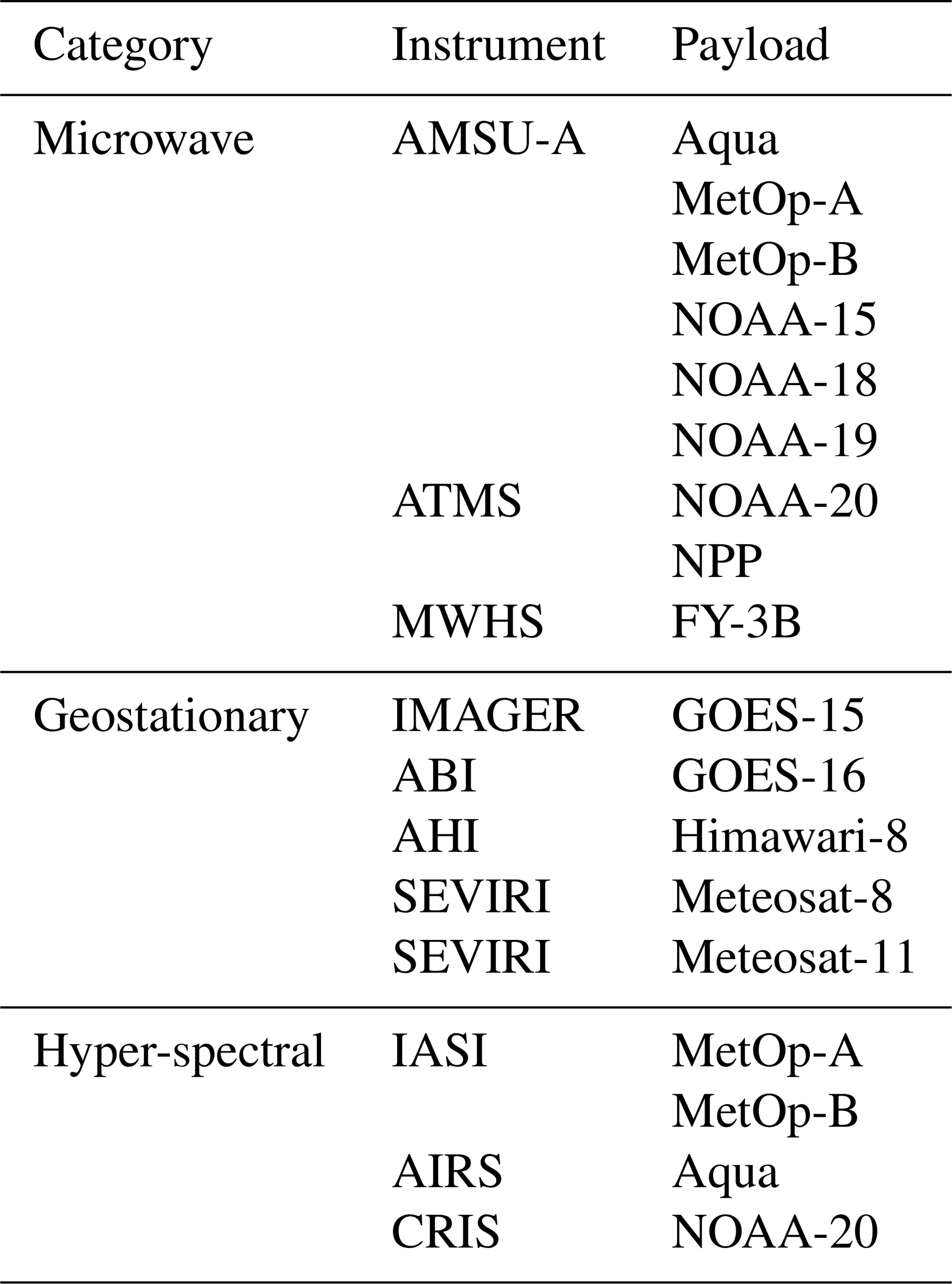
Table 1 The list of instruments used in clear-sky radiance assimilation is as follows: Advanced Microwave Sounding Unit-A (AMSU-A), Advanced Technology Microwave Sounder (ATMS), MicroWave Humidity Sounder (MWHS), Advanced Baseline Imager (ABI), Advanced Himawari Imager (AHI), Spinning Enhanced Visible and InfraRed Imager (SEVIRI), Infrared Atmospheric Sounding Interferometer (IASI), Atmospheric Infrared Sounder (AIRS), and Cross-track Infrared Sounder (CRIS).

4 Results

4.1 Experiments

To assess the differences between the current approach for the skin temperature analysis in the clear-sky radiance observation operator (TOVSCV) and the proposed approach (SKTECV), we ran two parallel experiments, one for each approach. For both experiments, we have a Northern Hemisphere summer period – July to September 2019, referred to as “JAS 2019” – and a Northern Hemisphere winter period – January to March 2020, referred to as “JFM 2020”. Each period is preceded by a spin-up of a few weeks. These experiments are based on the IFS cycle CY47R1 and RTTOV version 12.2 (Saunders et al., 2018).

4.1.1 Clear-sky radiance observations

The instruments providing clear-sky radiance observations and assimilated in the IFS cycle CY47R1 are presented in Table 1. In Sect. 1, we discussed that we carefully selected the channels in order to avoid those that are very sensitive to the surface. For the geostationary instruments, we only used the water vapour channels, which are rather weakly sensitive to the surface. The data over a grid cell where the model orography is higher than 1.5 km are also rejected. For the other infrared instruments, a situation-dependent screening is applied to identify channels strongly sensitive to the surface emission over land, and these channels are blacklisted. We do use near-window channels sensitive to the surface over the ocean but not over sea ice. Nonetheless, these are only used when the relevant channels are cloud-free, which excludes a large number of them.

A detailed usage of surface-sensitive microwave channels is presented in Table 1 of Bormann et al. (2017). For this study, we focus on the Advanced Microwave Sounding Unit-A (AMSU-A) instruments, which have channels near the 50 GHz oxygen absorption line, and on the MicroWave Humidity Sounder (MWHS) instruments, which have channels near the 183 GHz water vapour absorption line. The Advanced Technology Microwave Sounder (ATMS) instruments have channels for both frequencies.

The sensitivity to the surface and the type of information available from the assimilated microwave and infrared channels differs considerably, including the number of surface-sensitive channels assimilated. For the infrared sounders, many channels with relatively strong surface sensitivity are assimilated over the ocean from the hyper-spectral sensors, but many observations are screened out due to cloud contamination. The use of surface-sensitive channels is also more cautious over land. On the other hand, there is a wider range of microwave sounders available, with different overpass times, and these are less affected by cloud contamination. These characteristics will affect the response of the skin temperature estimation.

4.1.2 Resolution

The incremental formulation of the IFS 4D-Var means that each inner loop has a different resolution. Here, the outer loop has a TCo 399 horizontal grid (or spatial resolution of about 25 km; Malardel et al., 2016) and a vertical grid with 137 vertical levels. The inner loop horizontal grids are TL 95, TL 159, and TL 255 successively (or a spatial resolution of about 200, 125, and 80 km respectively), with the same vertical grid as the outer loop.

4.2 Skin temperature analysis

The key difference between the two approaches is the skin temperature analysis. Thus, we start by inspecting the skin temperature analysis in both experiments. First, we focus on the two-dimensional fields provided by the SKTECV experiment. Then, we compare the skin temperature analyses from the two experiments in the observation space, which is the space where the TOVSCV experiment provides its skin temperature analysis.

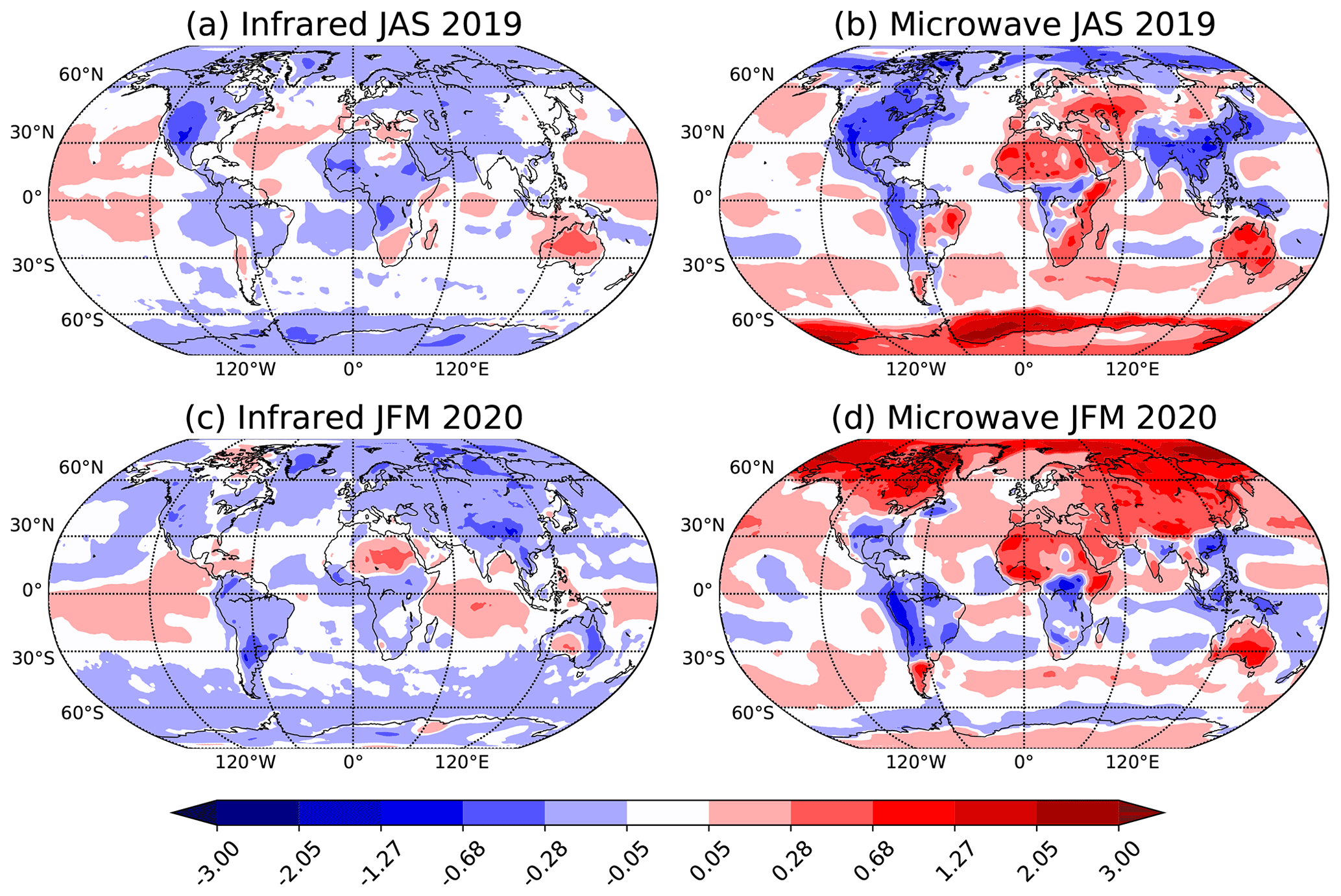
Figure 1 Time average of the skin temperature increment (in K) from the SKTECV experiment for (a, b) JAS 2019 and (c, d) JFM 2020 for (a, c) the infrared field and (b, d) the microwave field.

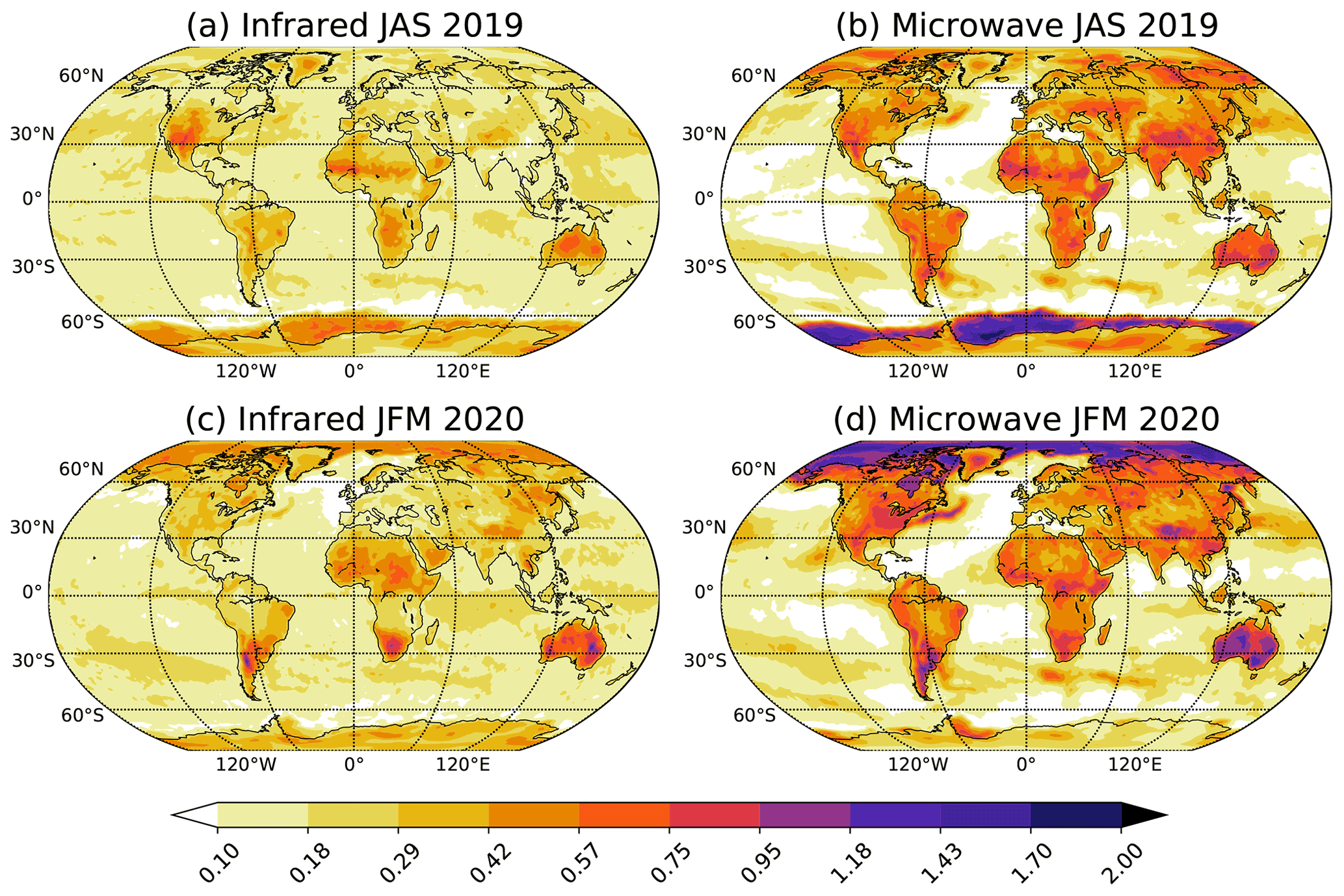
Figure 2 Standard deviation of the skin temperature increment (in K) from the SKTECV experiment for (a, b) JAS 2019 and (c, d) JFM 2020 for (a, c) the infrared field and (b, d) the microwave field.

4.2.1 Model space

The SKTECV approach starts from the model skin temperature as a background. The 4D-Var produces the analysis increment which is the optimal adjustment to the background and the new batch of observations. The temporal mean of the analysis increment is a proxy of the background bias. We computed the temporal mean of the analysis increment for the two periods and the two skin temperature fields for the SKTECV experiment (Fig. 1).

For the infrared field, the mean value is mainly under 0.3 K in absolute value. The difference between the two seasons is minimal. It appears that the model skin temperature provides a relatively unbiased background for the infrared skin temperature field. As discussed in Sect. 4.1.1, most of the actively assimilated infrared radiances have relatively weak surface sensitivity over land and sea ice. This limits the increments in these regions.

For the microwave field, there is a contrast between the ocean on one hand and the land and sea ice on the other hand. Over the ocean, the absolute value of the mean is mostly under 0.3 K. Elsewhere, where the SKTECV approach makes use of surface-sensitive microwave channels, the mean can reach absolute values of more than 3 K. Moreover, there are large differences between the two seasons. For example, there is a change of sign in the mean over sea ice in Antarctica or over Canada. The larger differences over land likely reflect that microwave frequencies can be sensitive to deeper subsurface layers, and this is not captured by using the model skin temperature as a background field. In addition, the specular assumption currently used in the radiative transfer calculations for microwave frequencies has been found to be suboptimal over snow and sea-ice areas, whereas diffuse, Lambertian reflection may be more appropriate (Karbou et al., 2006; Bormann et al., 2017). The specular assumption leads to viewing-angle-dependent biases, and these are partly compensated for by increments in the skin temperature. This likely contributes to the larger mean increments over Canada and northern Asia in winter.

From the time series of the analysis increment, we also computed the temporal standard deviation for the two periods and the two skin temperature fields (Fig. 2). This quantity is a proxy of the analysis activity: the larger the standard deviation, the larger the activity. The pattern of the standard deviation is similar for the two fields: the lowest values are found over the ocean (mostly under 0.3 K), and the largest values are found over sea ice (up to 2 K). This is expected, as the standard deviation of the background errors is lower over the ocean and the uncertainty is large over sea ice.

Over the ocean, the analysis is slightly more active for the infrared field than for the microwave field. For both, the activity is larger inside the subtropical gyres limited by the ocean currents, and the activity is larger in the region of the Gulf Stream current along the eastern American coast.

Over land and sea ice, the analysis is less active for the infrared field than for the microwave field, as expected from the blacklisting of the surface-sensitive channels of the infrared radiances. However, the standard deviation is higher than over the ocean which means that there is still some surface sensitivity in the remaining infrared radiances. The higher values over land for the microwave field can be explained by both the higher surface sensitivity and by the larger number of available instruments (providing more of the diurnal sampling). The activity is even larger over desert regions, where the diurnal cycle of the skin temperature can be strong, and around regions with high orography. Yet, the activity is the largest over sea ice.

4.2.2 Observation space

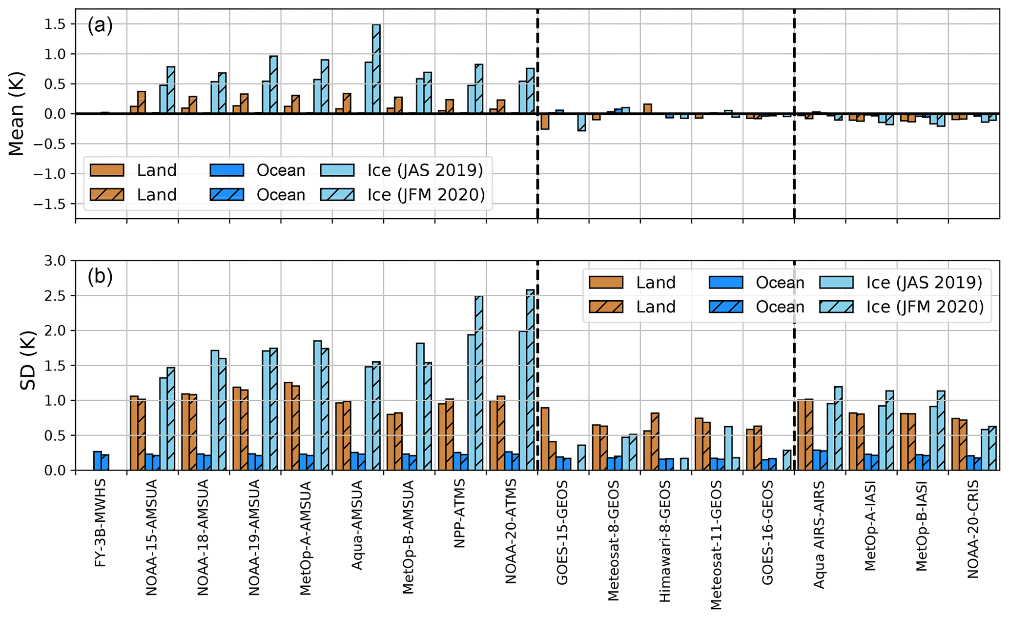
Figure 3 Mean (a) and standard deviation (b) of the skin temperature analysis difference between the SKTECV and the TOVSCV experiments for each instrument and for the two seasons: JAS 2019 (colour) and JFM 2020 (hatched colour). The difference is computed over the ocean, sea ice, and land (see legend). The left part of the plot shows the microwave instruments, the middle part of the plot shows the infrared instruments (geostationary), and the right part of the plot shows the infrared instruments (polar orbiting).

For each field of view of the radiance observations, the background and analysis values of the skin temperature are stored in the Observational DataBase (ODB; Fouilloux, 2009). For both experiments, we can extract the matching skin temperature analysis/background and compute the analysis increment for each experiment and the analysis difference (SKTECV minus TOVSCV) in observation space (time and location of each field of view). Figure 3 presents the mean and standard deviation of the analysis difference for each instrument, and for the two seasons. We also computed the mean of the analysis increment standard deviation by instrument type for each of the two experiments. All of the statistics are computed over three surface properties (land, ocean, and sea ice), as we previously saw that there are large differences between them.

Note that, due to instrument problems, the three lowest-peaking channels (5–7) of Aqua AMSU-A were not used over sea ice. This reduces the constraint of this instrument on its skin temperature analysis in the TOVSCV approach and reduces the constraint over sea ice to zero.

In the TOVSCV experiment, the geostationary infrared instruments have little sensibility to the surface; therefore, the analysis increment is close to zero on average and has little variability. Meanwhile, by construction, the average and variability in the SKTECV experiment are similar for all infrared instruments, and their values are constrained mainly by the hyper-spectral instruments.

We found a reduction in the analysis increment variability in the SKTECV experiment compared with the TOVSCV experiment except for the microwave instruments over the ocean. The reduction is a combined effect of the addition of spatial and temporal correlations and of using one field per instrument type in the SKTECV experiment. The increase over the ocean in the microwave instruments can be attributed to an increase in the temporal variability in the SKTECV experiment.

Over the ocean, the mean difference is close to zero for all instruments. The standard deviation is around 0.25 K, which is of the same order as the mean background error standard deviation. For the microwave instruments, this value is mostly driven by the SKTECV experiment for which the standard deviation values are around 250 % higher. Over land, the mean difference is also close to zero except for the microwave instruments during the JFM 2020 season, and the standard deviation is between 0.5 and 1 K, which is once again of the same order as the mean background error standard deviation.

This means that both approaches are similar in terms of skin temperature analysis over land and the ocean, except for microwave instruments during the JFM 2020 season over land. This difference largely originates from areas with large analysis increments over the Northern Hemisphere, as discussed earlier, for which local values can reach up to 3 K.

As the usage of the surface-sensitive channels for the infrared instruments is limited over sea ice, there is not much difference between the two approaches. The standard deviation of the difference is about 1 K, which is lower than the background error standard deviation. However, the standard deviation of the SKTECV experiment is about 50 % lower.

There is a bigger difference between the two approaches for the microwave instruments over sea ice. First, the mean difference is between 0.5 and 1 K. This difference comes from the SKTECV experiment for which the mean increment is positive, whereas the mean increment has values close to 0 K for the TOVSCV experiment (not shown).

Due to the difference in the background error standard deviation between the two experiments, the SKTECV experiment has a less active skin temperature analysis by about 7 % (JAS 2019) and 20 % (JFM 2020). The largest standard deviation values of the skin temperature analysis difference over sea ice compared with the other surface types are, thus, partially due to larger variability in the increments in the TOVSCV experiment and also to larger variability over this surface type.

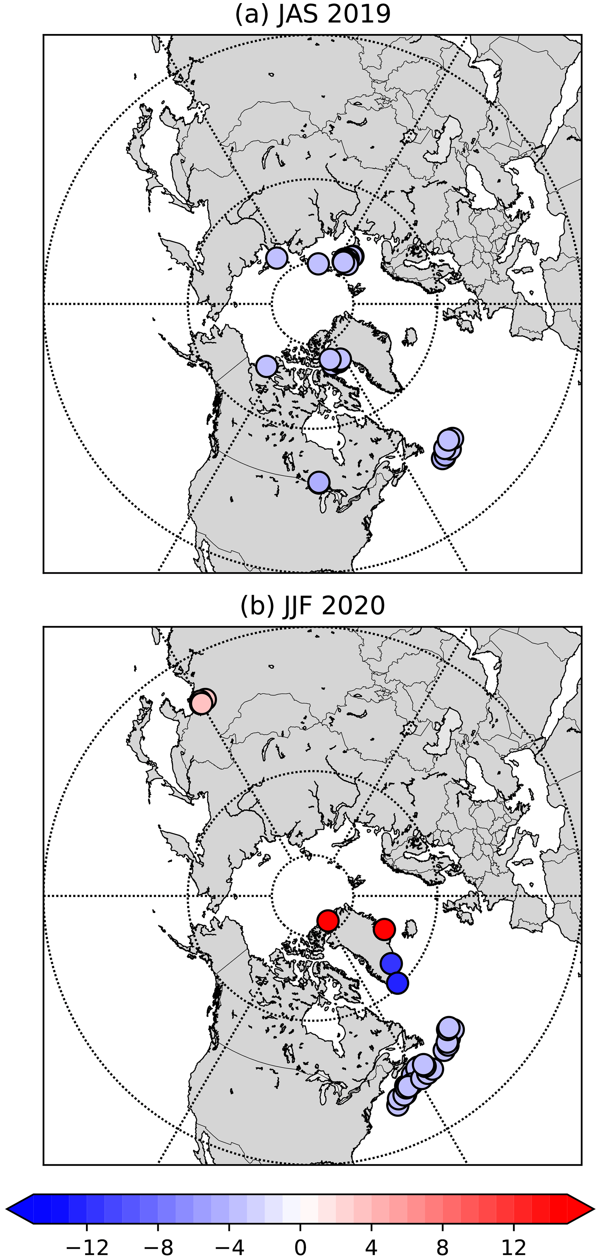
Figure 4 Difference in the skin temperature analysis in observation space (in K) between the experiment and the control when the difference exceeds 3 background error standard deviations and for NOAA-20-ATMS. Bluish colours denote SKTECV values lower than TOVSCV values, and reddish colours denote SKTECV values greater than TOVSCV values. The time periods shown are (a) JAS 2019 and (b) JFM 2020.

4.2.3 Outliers

With the exception of sea ice, we can conclude that the two approaches are similar on average. We believe that the SKTECV approach could be beneficial for particular situations, as the skin temperature is better constrained through several instruments at the same time as well as via the spatial and temporal correlations of the background error. The TOVSCV experiment, in contrast, allows, for example, for possible inaccuracy in the surface emissivity or in the cloud screening, or viewing-angle-dependent biases from the specular assumption (when relevant) to be aliased into skin temperature increments. Thus, we investigated the cases for which the skin temperature analysis is significantly different between the SKTECV and TOVSCV experiments, as this could point to situations where the skin temperature in TOVSCV compensates for other large errors. We searched for the outliers defined as scenes where the skin temperature analysis difference is larger than a threshold t and simultaneously the skin temperature background difference is larger than $t/\mathrm{2}$.

We chose the threshold to be equal to 3 times the local value of the skin temperature background error standard deviation from the TOVSCV experiment. The threshold is then situation dependent over land but constant over the ocean and sea ice with respective values of 3 and 22.5 K.

For the infrared instruments, we did not find any outliers with this criteria. For the microwave instruments, all of the outliers were found in the Northern Hemisphere, and most of them were located over the ocean or near the coastline (Fig. 4). This is linked to the usage of the background error standard deviation from the EDA over the ocean in the SKTECV experiment which allows the skin temperature increments to be larger. For instance, for the outliers located on the East Coast of the USA, the sea surface uncertainty is higher than 1 K and is associated with the Gulf Stream. The uncertainty is also large in the Arctic region. Looking at these outliers in more detail, the larger increment in the SKTECV experiment allows for the analysis to better fit channel 6 of ATMS (not shown). Nevertheless, because it concerns only few points, this does not have an overall significant impact on the analysis.

If we change the threshold to a lower value, we start to have outliers over sea ice. For this surface type, the skin temperature increment is always larger in the TOVSCV experiment, as expected from the difference in the value of the background error standard deviation. We also start to have outliers over land in the regions where the skin temperature is very sensitive to the meteorological conditions. Small differences in the weather parameters between the two experiments can cause differences in model skin temperature close to or larger than the threshold in these regions. The assimilation processes of both experiments were then usually not able to change the skin temperature enough to bring their analyses close to each other.

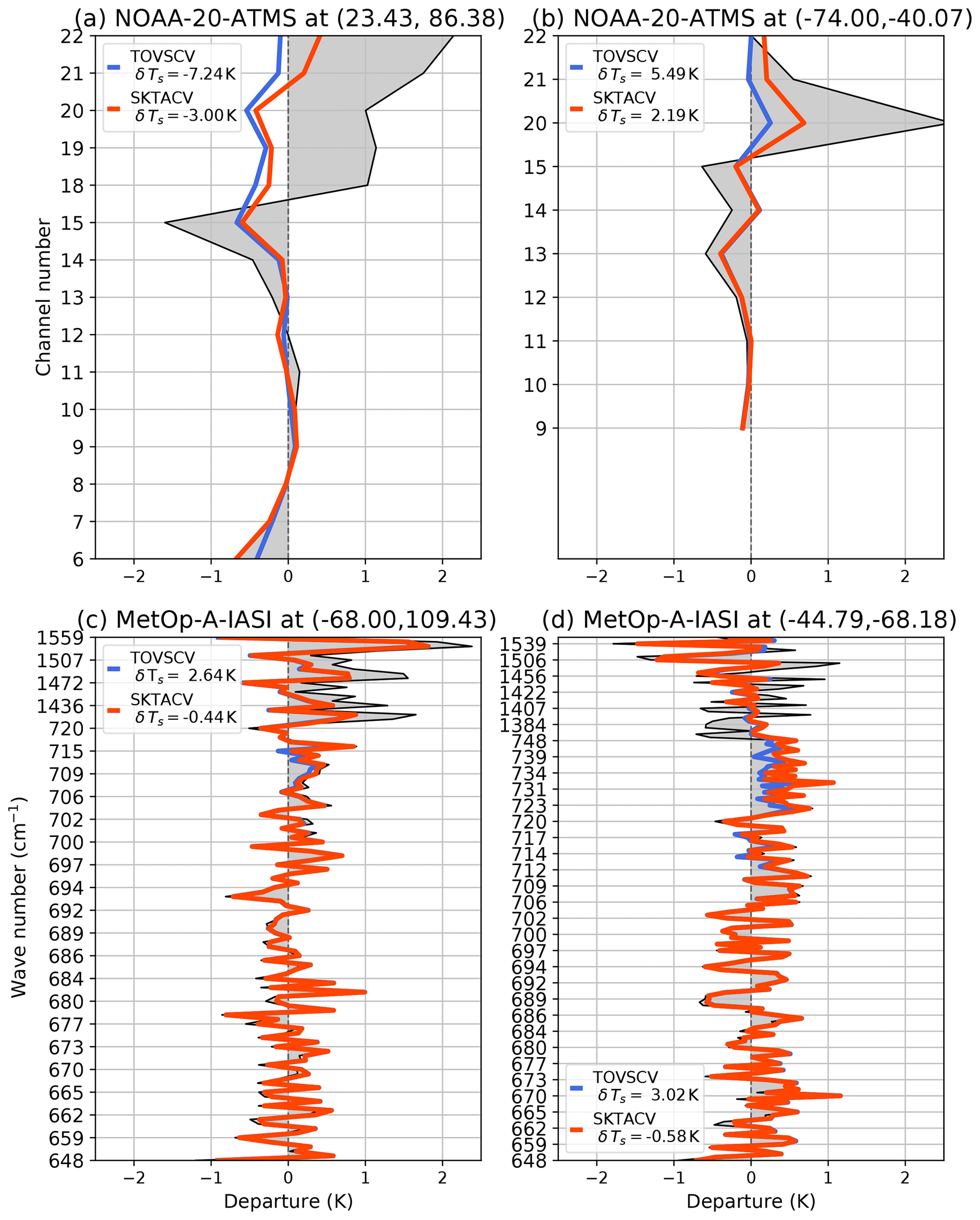
Figure 5 First-guess (grey shading) and analysis (coloured lines) departures (in K) for ATMS (a, b) and IASI (c, d) for four particular scenes; see the plot titles for the location (latitude, longitude) of the scenes. Blue denotes departures from the TOVSCV experiment, and red denotes departures from the SKTECV experiment. In the legend, δT_s is the value of the skin temperature increment.

In conclusion, we did not find any scenes for which the TOVSCV experiment seems to excessively boost the skin temperature increment to compensate for other errors.

4.2.4 Cases study

To illustrate the difference in behaviour between the two approaches, we detail four particular scenes in the following: two for the ATMS instrument (microwave) and two for the Infrared Atmospheric Sounding Interferometer (IASI) instrument (infrared). For each scene, we present the first-guess and analysis departures in radiance space (Fig. 5).

The scenes are from the very first assimilation cycle of the summer period. The background values for the atmospheric variables and for the skin temperature are the same for the two approaches. This facilitates the interpretation of the differences between them. Nonetheless, one has to be careful not to attribute the observed differences in the analysis departures only to the skin temperature analysis at the location of the scene. For a given scene, a difference in the skin temperature analysis in the surrounding model grid cells creates a difference in the atmospheric variables in those grid cells and, subsequently, in the grid cell of the scene due to the spatial covariances of the atmospheric variables background error.

For the first ATMS scene, which is over land, the TOVSCV experiment produces a large skin temperature increment (−7.24 K), larger than the one from the SKTECV experiment (−3 K). This allows the TOVSCV analysis to better fit the measurements for surface-sensitive channel 6 than the first guess and than the SKTECV analysis, but results in a worse fit for channels 18 to 20, compared with the SKTECV analysis. For the second scene, which is over sea ice, none of the lower-tropospheric temperature-sounding channels are assimilated. The TOVSCV experiment then produces a large skin temperature increment (5.5 K) that allows its analysis to better fit the measurements for channels 20 to 22 compared with the SKTECV analysis, for which the skin temperature increment is smaller (2.2 K).

For the TOVSCV experiment, the skin temperature for each field of view is only constrained by its background in opposition to the atmospheric variables that are also constrained by surrounding observations due to the spatial correlation in the background error. Therefore, the skin temperature can be purposely adjusted to improve the fit to the channels that are sensitive to the surface. This is illustrated in the two ATMS cases where the analysis can lead to large skin temperature increments. If present, the lower-tropospheric temperature-sounding channels will be the more impacted as, for example, the prescribed observation error is more than 5 times lower for channel 6 than for channels 18 to 22.

In contrast, in the SKTECV experiment, the skin temperature is also constrained by adjacent observations via the skin temperature background errors, reducing the strong response to one particular observation.

The first IASI scene is over Antarctica, while the second scene is over land. For both scenes, the skin temperature increments from the SKTECV analysis are small (−0.4 and −0.6 K respectively). The increments from the TOVSCV analysis are larger (2.6 and 3 K respectively), which improves the analysis fit to observation for the wave numbers between about 710 and 750 cm⁻¹, corresponding to lower-tropospheric sensitive channels. For the first scene, despite the large skin temperature increment, the analysis fit is only marginally improved, which may suggest that the skin temperature adjustment compensates for other errors.

4.3 Meteorological analysis

On average, the skin temperature analysis is similar for the two approaches. We now assess how the two analyses compare for other variables.

4.3.1 Analysis fit to observations

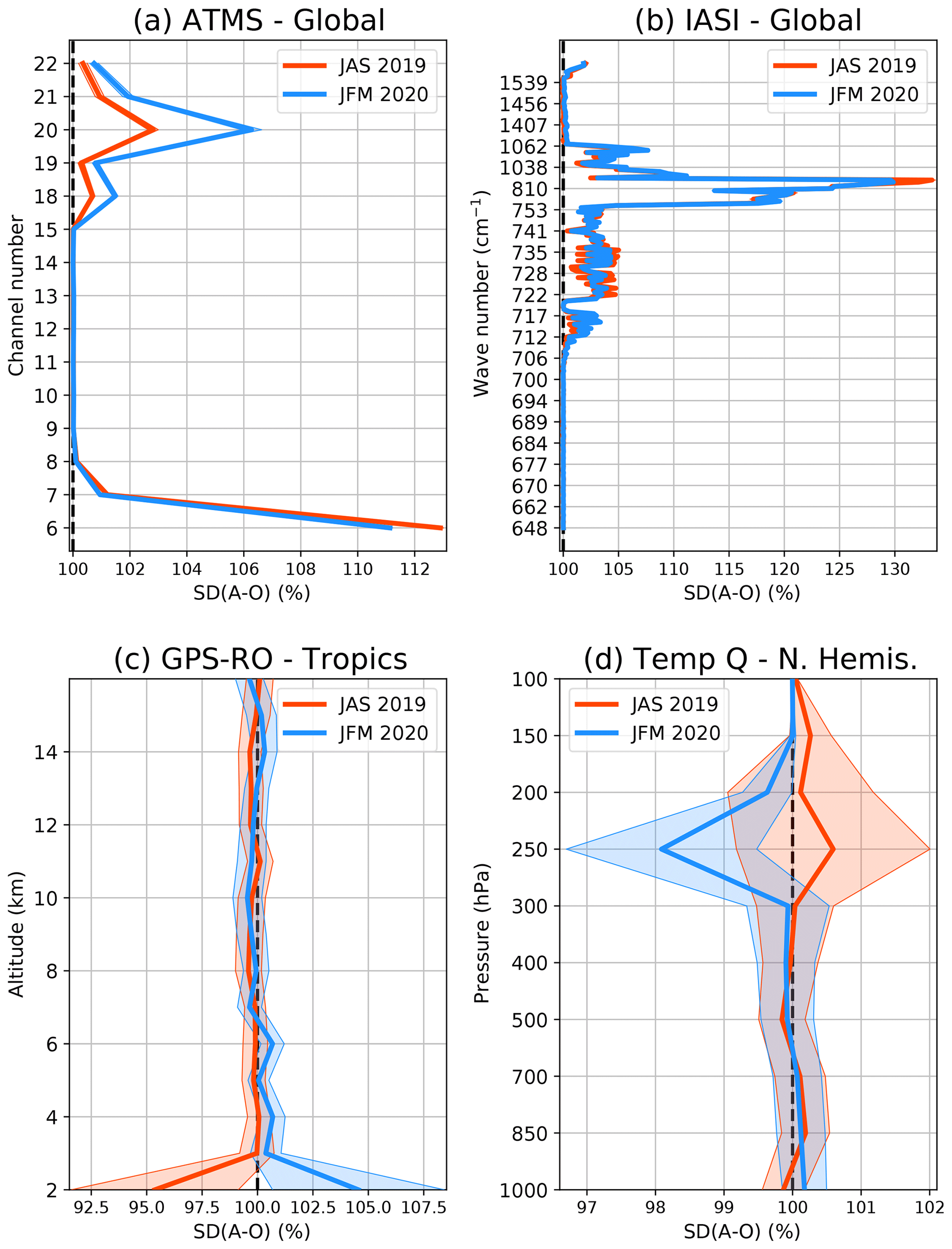
Figure 6 Normalised analysis fit to observations (in %) for various observation types (see panel headings) for JAS 2019 (red) and JFM 2020 (blue). The shaded area represents the variability (1 standard deviation).

We define the analysis fit to observations as the standard deviation of the SKTECV analysis departure (analysis minus observation) normalised by the standard deviation of the TOVSCV analysis departure. If the analysis fit to observations is lower than 100 %, the SKTECV analysis is labelled as closer to the observations. Otherwise, the TOVSCV analysis is labelled as closer to the observations.

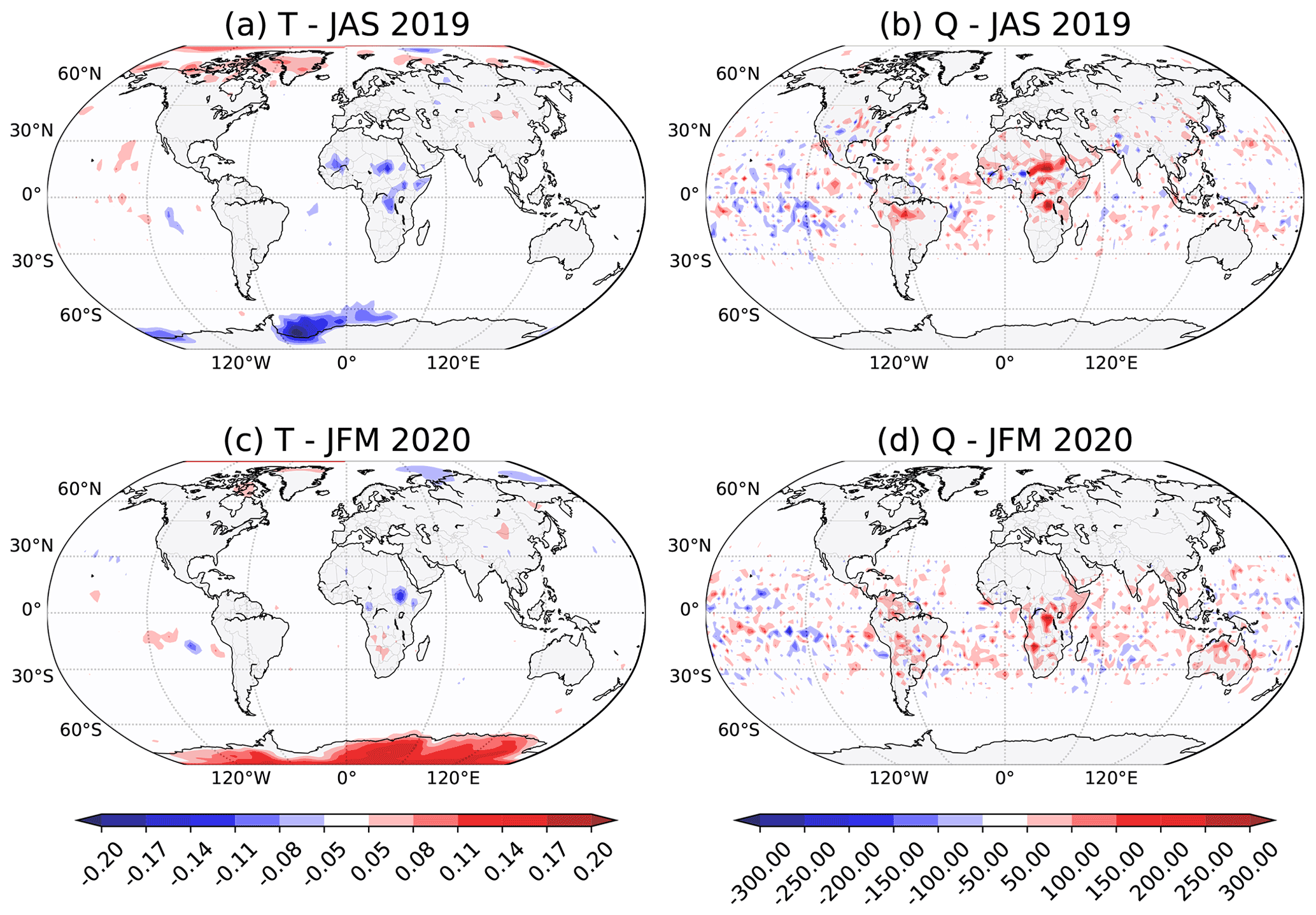
Figure 7 Time average difference between the SKTECV and the TOVSCV analyses at 850 hPa for (a, b) JAS 2019 and (c, d) JFM 2020 for (a, c) the temperature (in K) and (b, d) the specific humidity (in µg g⁻¹). Note that when the 850 hPa level is below the surface, the lowermost model level is used.

We first present the analysis fit to the radiance observations. By design, the skin temperature analysis impacts the radiance observation operator. This impact is detectable in the analysis projected in the radiance observation space through the observation operator. We present only the results for ATMS and IASI because these two examples are representative of the other microwave and infrared instruments.

For ATMS, the analysis fit is 10 % larger for channel 6 and up to 6 % larger for channels 18 to 22 (depending on the season) in the SKTECV experiment compared with the TOVSCV experiment. This is likely linked to the mechanism described in the case study. The TOVSCV experiment uses the skin temperature to better fit the measurements for channel 6 when assimilated and for channels 18 to 22 otherwise.

For IASI, the difference between the two experiments is larger than for ATMS for the channels sensitive to the surface. For the window channels around 810 cm⁻¹, the analysis fit of the SKTECV experiment is about 30 % larger (Fig. 6b). The fit is also larger, although by less than 5 %, for the lower-tropospheric sensitive channels (around 700–800 cm⁻¹). This is in accordance with the previously studied case: the TOVSCV experiment uses the skin temperature to better fit the measurements for these channels. For the geostationary infrared instruments, the analysis fit to observations is also slightly larger for the SKTECV experiment, by around 0.25 % for JAS 2019 and around 0.5 % for JFM 2020 (not shown).

From these results alone, it is not possible to say which of the two systems performs better. On the one hand, the findings may indicate that the TOVSCV experiment uses the skin temperature to over fit the radiance observations, either due to overly large assumed background errors or possibly by aliasing scene-dependent errors with suitable spectral signatures into skin temperature increments (e.g. cloud-screening errors or emissivity/specularity errors). On the other hand, the results may indicate that the skin temperature is too strongly constrained in the SKTECV experiment which prevents the analysis from fitting the radiance observations more closely. Either way, the temperature and humidity analyses are expected to be different from the surface, up to the middle troposphere. This can be assessed with the analysis fit to other observations.

We found that the SKTECV temperature analysis is generally slightly closer (by less than 0.5 %) to global positioning system radio occultation (GPS-RO), sondes, and aircraft data for JAS 2019. For JFM 2020, the results are more mixed. The largest difference was detected for the fit to the GPS-RO data in the lower troposphere and over the tropics, where there is a contrasting behaviour between the two seasons. The SKTECV temperature analysis has a closer fit, by about 5 %, in JAS 2019 and a looser fit, by about 5 %, in JFM 2020 (Fig. 6c). It is not clear where this difference comes from, as no such differences were found in the analysis fit to other observations in the tropics.

The difference in the humidity analysis fit is mostly not statistically significant when compared with the sondes and aircraft data. The humidity analysis fit values are within ±0.5 %. The exception is for the analysis fit to sondes data in the upper troposphere (around 250 hPa) for JFM 2020: the SKTECV humidity analysis is significantly closer to the observation by 2 % (Fig. 6d). This is the region where ATMS channels 18 to 22 are sensitive to humidity and where the TOVSCV analysis is closer to the ATMS observations. This suggests that the TOVSCV approach may use the skin temperature to compensate for inaccuracy in the surface emissivity in the Northern Hemisphere for JFM 2020, allowing the analysis to be closer to ATMS channels 18 to 22 but also putting the humidity analysis further away from the radiosondes data.

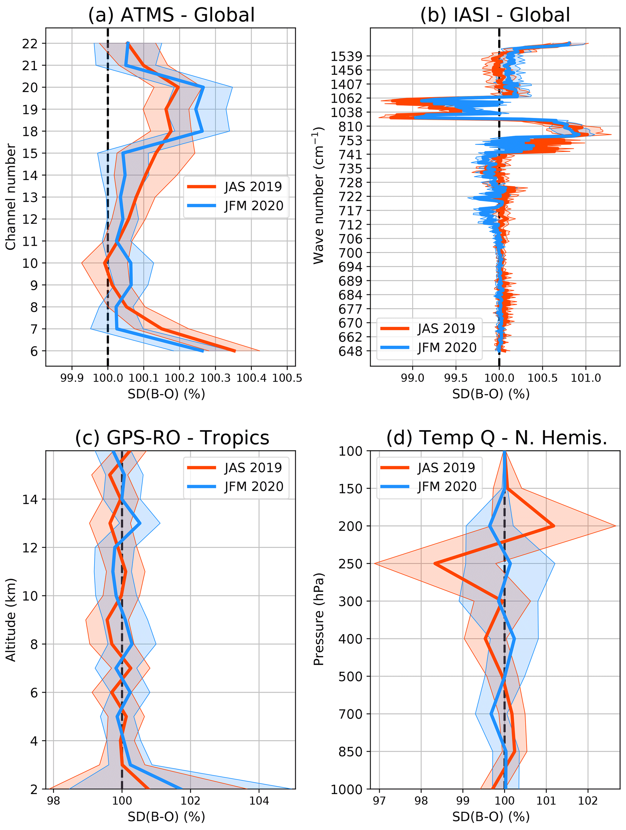
Figure 8 Normalised first-guess fit to observation in (%) for various observation types (see panel headings) for JAS 2019 (red) and JFM 2020 (blue). The shaded area represents the variability (1 standard deviation).

4.3.2 Mean analysis difference

We saw that the analyses from the two approaches differ when compared with observations. Here, we directly compare the two analyses in physical space. We found that the mean atmospheric states are very similar in the two analyses, and the few differences appear in the lower atmosphere only. In this region, the mean temperature analyses mainly differ by less than 0.05 K, and the mean humidity analyses differ by less than 50 µg g⁻¹.

The largest differences for temperature are found in the polar regions. For example, at 850 hPa, when compared with the TOVSCV experiment, the SKTECV experiment is warmer in the Arctic region and cooler in the Antarctic region in JAS 2019, whereas the opposite is found in JFM 2020 (Fig. 7a, c).

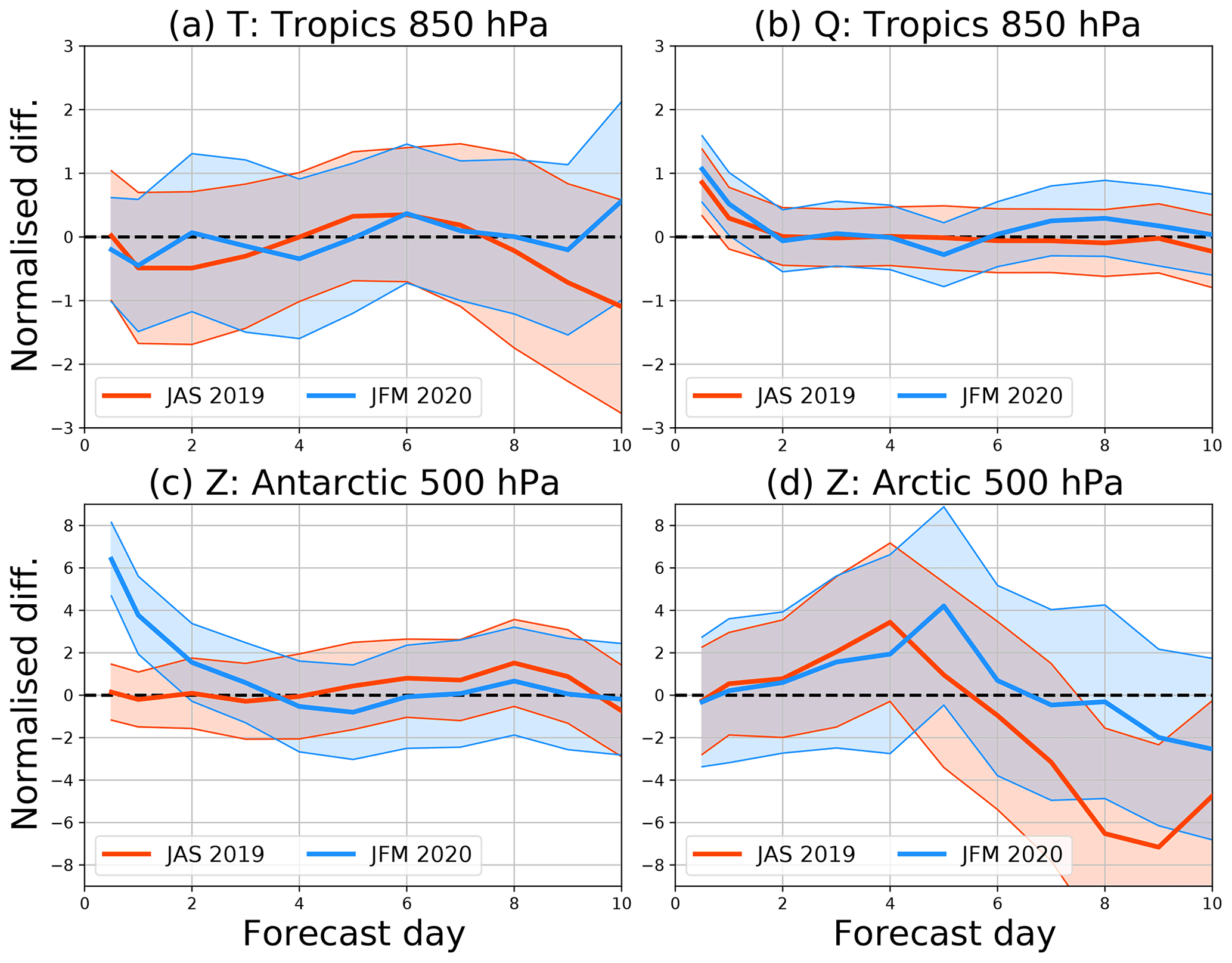
Figure 9 Normalised difference in root mean square error (full line, in %) between the SKTECV and the TOVSCV experiments, when compared with the operational analyses, and the associated uncertainty (coloured shading). Red denotes JAS 2019, and blue denotes JFM 2020. See the panel headings for the parameter and region plotted.

We previously found that the mean increment for the microwave instruments is positive and large in the winter season (JAS 2019) over the Antarctic region, especially in the Weddell Sea. In this area, the analysis tends to warm the atmosphere at 850 hPa. By increasing the skin temperature for the microwave instruments, the SKTECV analysis reduces the warming of the atmosphere compared with the TOVSCV analysis. This is a very limited area, and it is difficult to assess which analysis is better.

Still over the Antarctic region but for the summer season (JFM 2020), the mean increment for the microwave instruments is close to zero, and the skin temperature analysis is not very active compared with that from the TOVSCV experiment. Both analyses tends to warm the atmosphere in the above-mentioned region. As it has a more active skin temperature analysis, the TOVSCV experiment reduces the warming of the atmosphere compared with the SKTECV analysis. This difference makes the SKTECV temperature analysis slightly closer to the radiosonde measurements than the TOVSCV one (not shown).

There are also some local differences in the mean temperature analysis in the tropical region of Africa. This could be linked to errors in the emissivity that are propagated to the skin temperature in the TOVSCV experiment. Moreover, there is a moistening of the tropics on average in the SKTECV experiment compared with the TOVSCV experiment (Fig. 7b, d). This also makes the SKTECV humidity analysis slightly closer to the radiosonde measurements than the TOVSCV one (not shown).

The discrepancy in the temporal standard deviation of the analysis between the two experiments informs us of the activity of the analysis. For the temperature, we found that the difference is negligible, with maximum values of 0.05 K detected in the polar regions. For the humidity, the difference is also small. The largest difference is found in the tropics, close to the surface, where the SKTECV experiment has a lower standard deviation (by a maximum of 20 µg g⁻¹).

To summarise, the two analyses are very similar on average, with no important difference between the two seasons. The main differences are located in the polar regions, where the temperature in the lowest model levels is warmer during the summer season in the SKTECV analysis. There are also other differences in the tropics, close to the surface, where the SKTECV analysis is slightly moister and slightly less active.

4.4 Short-range forecast

The atmospheric analysis serves as an initial condition for the short-range forecast that is used as the first guess for the next assimilation cycle. This first guess is compared to all available observations to compute the first-guess departure. The standard deviation of the first-guess departure gives information on the quality of the first guess. Here, we compute the normalised first-guess fit to observation which is the standard deviation of the first-guess departure of the SKTECV experiment normalised by standard deviation of the first-guess departure from the TOVSCV experiment. For a value lower or greater than 100 %, the SKTECV first guess is labelled as better or worse than the relevant observations respectively.

For the ATMS instrument, the SKTECV first guess is slightly worse (by up to 0.3 %) for the channels that are sensitive to the surface (Fig. 8a). The only exception is for the Northern Hemisphere in JFM 2020 for which the first guess is 0.1 % better (not shown). Combined with the finding that the SKTECV analysis fit to ATMS observations is larger than the TOVSCV analysis fit, the result suggests that, on average, the skin temperature may be too strongly constrained in SKTECV for the microwave instruments.

For the IASI instrument, there is a dipole in the normalised first-guess departure (Fig. 8b). The first guess is better by up to 1 % for the ozone channels and worse by up to 1 % for the window channels. This phenomenon has already been observed and is under investigation (Cristina Lupu, ECMWF, personal communication, 2020). Here, we can only conclude that even if the SKTECV approach largely affects the analysis fit to hyper-spectral infrared measurements, it is neutral when it comes to the first-guess fit.

When compared with other instruments, the difference in the standard deviation of the first-guess fit is mostly not statistically significant, as illustrated with the GPS-RO data in Fig. 8c. The only statistically significant difference comes from the comparison against humidity measurements from radiosondes at 250 hPa in the Northern Hemisphere, where the SKTECV experiment is better for JAS 2019 (Fig. 8d). This is the region where we saw a better fit for the SKTECV experiment in the analysis fit to humidity, although this was for JFM 2020.

4.5 Forecast scores

For assessing the forecast quality at up to day 10, we use the operational analysis as the reference to compute the forecast error. The operational analysis is assumed to be our best knowledge of the global atmospheric state at a given time. Because the operational analysis has a TCo 1279 horizontal grid (spatial resolution of about 9 km), we do not expect it to favour the TOVSCV experiment, even if it uses the TOVSCV approach.

The metric that we are using is the normalised difference in the root mean square error (RMSE) of the forecast error for forecast lead times between 1 and 10 d (Geer, 2016). If the normalised difference is negative or positive for a given lead time, the forecast from the SKTECV experiment is labelled as better or worse than the one from the TOVSCV experiment for this lead time respectively. If the 0 % line is outside the uncertainty range, the result is statistically significant; otherwise, it is not. These scores are computed by region and for each parameter.

Here, we focus on the tropics and the polar regions, below 60^∘ S and above 60^∘ N, where the largest differences in the analysis were observed. In the tropics at 850 hPa, the normalised difference in the RMSE is within 0.5 % for humidity, and within 1 % for temperature, for all forecast ranges and without any statically significant signal (Fig. 9a, b).

For the polar regions, we discuss the normalised difference in the RMSE for the geopotential (Z) at 500 hPa, as it summarises the quality of the forecast from the surface up to 500 hPa (Fig. 9c, d). The first statistically significant difference is in Antarctica, in winter and up to day 3. The forecast error is up to 6 % larger for the SKTECV experiment. This is also confirmed by the verification against observations, but the increase in error is then between 1 % and 2 %. This increase comes primarily from a larger mean error in the SKTECV experiment linked with a sightly warmer analysis, as discussed previously. The second statistically significant difference is over the Arctic where the SKTECV forecast is 3 % to 5 % better after day 7. This improvement is confirmed by the comparison with observations, although without statistical significance.

5 Conclusions

During the assimilation process, the skin temperature is adjusted in the IFS along with all of the atmospheric variables in order to produce a simulated radiance that best fits the observed radiance. This is achieved by extending the atmospheric 4D-Var control vector with a set of skin temperature values defined in observation space for each field of view. This approach is known as TOVS control variable (or TOVSCV).

The TOVSCV approach is suboptimal, as without spatial or temporal constraints, each individual skin temperature value is adjusted independently. In this paper, we proposed an enhanced approach, referred to as SKTECV, that allows for the definition of these spatial and temporal correlations in model space in a similar fashion to all of the other variables of the analysis state vector. The TOVSCV and SKTECV estimates of skin temperature agree fairly well overall, with differences mostly below the errors assigned to the background skin temperature values. This may suggest that aliasing of other errors in the skin temperature errors is not a major issue, and the screening applied to the affected radiances performs well in this respect.

By constraining the skin temperature analysis more strongly, the SKTECV analysis does not fit the radiance observations as much as the TOVSCV analysis for the channels sensitive to the surface and to the lower troposphere. Compared with other independent observations, there is no statistically significant difference between the two analyses. Furthermore, the two analyses and forecasts are not significantly different, on average, outside the polar regions.

The differences in the polar regions come mainly from the microwave instruments, for which the skin temperature analysis over sea ice is, on average, 0.5 to 1 K warmer depending on the season and instrument. Moreover, there is more variability in the skin temperature analysis in the TOVSCV experiment than in the SKTECV one, which is a consequence of the large difference in the value of the background error standard deviation over sea ice between the experiments.

The sensitivity of the microwave instruments to the surface is deeper than the layer represented by the model skin temperature. Therefore, using the model skin temperature as a background is not optimal. This is confirmed by the time average of the analysis increment of the microwave fields which has values of up to 3 K. We are currently investigating how to use the microwave skin temperature analysis from this study to obtain a better background and address the bias issue.

Changing the background value of skin temperature will change the first guess in radiance space and may also change the usage of the microwave observations. For example, our quality control tends to reject a significant portion of microwave data over deserts or snow-covered regions because of overly large biases (Lawrence et al., 2019). If we can improve our skin temperature background field, we may be able to reduce these biases and increase the number of assimilated radiances. A better skin temperature background should also lead to better dynamic emissivity estimates, resulting in further improvements.

Here, we considered two separate skin temperature fields. This can be further refined, as different channels within a category can have a different sensitivity to the surface. For instance, low-frequency channels are sensitive to a deeper surface layer than high-frequency channels for the microwave instruments. For example, we could separate channels 6–9 (50 GHz) from channels 18–22 (183 GHz) for ATMS. Moreover, we may be able to add more channels that are currently blacklisted because they were found to be problematic due to their sensitivity to the surface. For instance, for the infrared instrument, we could stop removing channels that are strongly sensitive to the surface over land and start using near-window channels sensitive to the surface over the sea ice.

Having the skin temperature as fields on the same grid as the atmospheric temperature will also allow for the introduction of a background error correlation between them following the approach of Garand (2004). Finally, the availability of a temporally and spatially consistent analysis of skin temperature can also be seen as an attractive by-product of the SKTECV method. These skin temperature analysis fields can drive further improvements in the estimation of physically connected fields (e.g. sea surface temperature, land surface temperature, sea-ice temperature).