Modeling of land–surface interactions in the PALM model system 6.0: land surface model description, first evaluation, and sensitivity to model parameters

In this paper the land surface model embedded in the PALM model system is described and evaluated against in situ measurements at Cabauw, Netherlands. A total of 2 consecutive clear-sky days are simulated, and the components of surface energy balance, potential temperature, humidity, and horizontal wind speed are compared to observations. For the simulated period, components of the energy balance are consistent with daytime and nighttime observations, and the daytime Bowen ratio also agrees fairly well with observations. The model simulates a more stably stratified nocturnal boundary layer than the observations, and near-surface potential temperature and humidity agree fairly well during the day. Moreover, a sensitivity analysis is performed to investigate dependence of the model on land surface and soil specifications, as well as atmospheric initial conditions, because they represent a major source of uncertainty in the simulation setup. It is found that an inaccurate estimation of leaf area index, albedo, or initial humidity causes a significant misrepresentation of the daytime turbulent sensible and latent heat fluxes. During the night, the boundary-layer characteristics are primarily affected by surface roughness and the applied radiation schemes.

1 Introduction

The land surface influences atmospheric dynamics significantly through the exchange of energy, mass, and momentum. Therefore, an accurate representation of surface–atmosphere interactions is essential for any numerical modeling of the atmospheric boundary layer (Garratt, 1993; Betts et al., 1996). More specifically, surface roughness as well as sensible and latent heat fluxes at the surface act as the lower boundary condition for the momentum, temperature, and humidity equations in the atmosphere, respectively. If this information is not available, it is necessary to parameterize the land surface processes with a land surface model (LSM). In simple terms, the input to an LSM is the type of surface, vegetation, and soil, as well as the radiative forcing. Based on that, LSMs solve the surface energy budget equation by means of a set of prognostic equations for the surface temperature and compute soil moisture and temperature in a multilayer soil model. Nevertheless, the results strongly depend on the input data (e.g., Avissar and Pielke, 1989).

LSMs are required in various numerical setups, e.g., when observational data for the sensible and latent heat fluxes are unavailable or do not adequately reflect the complexity of the landscape; in weather forecasting, it is natural to use a prognostic approach. Moreover, the use of an LSM allows us to study surface–atmosphere interactions on turbulent timescales across the entire domain. The temporal and spatial scales affect feedback effects, e.g., between mesoscale circulations and underlying heterogeneous surfaces (e.g., Patton et al., 2005; Huang and Margulis, 2010), between clouds and radiation (Lohou and Patton, 2014; Horn et al., 2015), and in cities where shadows of buildings are another reason for highly heterogeneous heat fluxes.

The PALM model system (formerly an abbreviation for Parallelized Large-eddy Simulation Model; Maronga et al., 2015, 2020) has been applied for studying a variety of atmospheric boundary-layer flows for about 20 years. Since 2015, PALM has come with a fully interactive LSM. Originally, it was designed similar to the LSM in the large-eddy simulation (LES) model DALES (Heus et al., 2010), which contains parameterizations from the TESSEL/HTESSEL scheme (Viterbo and Beljaars, 1995; van den Hurk et al., 2000; Balsamo et al., 2009, 2011), but also some found in the ISBA model (Noilhan and Mahfouf, 1996) and own extensions. The LSM in PALM was first described by Maronga and Bosveld (2017) and has been used with respect to radiation fog by Maronga and Bosveld (2017) and Schwenkel and Maronga (2019), also including Cabauw (Netherlands) data for evaluation. Recently, it has also been employed in urban environments (see first results in Maronga et al., 2020).

Other coupled LES–LSM implementations are found in, e.g., UCLA-LES (Huang et al., 2011), ICON-LEM (Dipankar et al., 2015), and the WRF model (Skamarock et al., 2019) in LES mode coupled to NOAH-LSM (Chen and Dudhia, 2001). In early literature, the focus of coupled LES–LSM studies was mainly to analyze the feedback effect that creates heterogeneity at the surface (e.g. Patton et al., 2005; Huang et al., 2009; Huang and Margulis, 2010; Brunsell et al., 2011). Today, most studies require the coupled LES–LSM approach to simulate realistic cases, e.g., in the urban environment or for wind turbine applications. As the methodology gains a foothold in engineering and industry, it is becoming increasingly important for the embedded land surface representation in PALM to reflect reality (Maronga et al., 2020).

This paper is part of a series featuring different parts of the PALM model system 6.0 in this special issue. For the user, a systematic sensitivity test of relevant land surface parameters with the LSM in PALM is of particular interest. In the present study, we evaluate the LSM embedded into PALM against Cabauw data for a selected period with clear-sky conditions and limited large-scale advection. Through this we ensure as far as possible that the developing boundary layer is not affected by non-local processes, which we neglect in the simulations of this study. Furthermore, we determine key parameters that influence the diurnal cycle in a coupled LES–LSM framework. The model sensitivity is analyzed by means of a comprehensive set of simulations varying land surface and soil parameters individually. Therewith, the present study complements the earlier work of Maronga and Bosveld (2017), who focused on the nocturnal boundary layer with developing radiation fog.

Section 2 of the paper describes physical and technical aspects of the LSM in PALM. Section 3 provides information about the Cabauw Experimental Site for Atmospheric Research (CESAR; Monna and Bosveld, 2013) and the observations used. Section 4 describes the model setup and initialization and gives a complete list of simulations conducted. Section 5 outlines the results of the sensitivity study and discusses the validity and limitations of the LSM. Finally, Sect. 6 draws the summary and conclusions and gives an outlook.

2 Description of the land surface model (LSM) in PALM

The specific implementation of PALM's LSM, which is derived from the HTESSEL scheme, is described below. It consists of a solver for the energy balance of the Earth's surface in combination with a multilayer soil scheme. The scheme was initially designed for vegetated surfaces and bare soil only, but it has since been adapted for paved surface materials like asphalt and concrete; a simplified version for inland and seawater surfaces has also been added. A tile approach is available for vegetated surfaces, in which the surface is a fraction of bare soil and a fraction covered with vegetation. Furthermore, the LSM has a liquid water reservoir on plants and soil to store and evaporate liquid water from precipitation interception and dew formation. A liquid water reservoir is also available when the surface type is set to pavement, representing the ability of impervious surfaces to store a limited amount of precipitated water on the surface. For further details, see also Viterbo and Beljaars (1995), van den Hurk et al. (2000), Balsamo et al. (2009, 2011), and the literature referenced therein.

2.1 Energy balance solver

The energy balance is calculated as

$$\begin{array}{}\text{(1)}& {\displaystyle \frac{\mathrm{d}{T}_{\mathrm{0}}}{\mathrm{d}t}}{C}_{\mathrm{0}}=R_{\mathrm{n}}-H-LE-G,\end{array}$$

where C₀ and T₀ are the heat capacity and radiative temperature of the surface, respectively. Note that C₀ is zero by default in the case of surfaces covered by vegetation or water surfaces, for which it is assumed that T₀ is the temperature of a skin layer covering the surface that does not have a significant heat capacity, which we think is a valid approach for low vegetation like grass. The heat capacity is fully customizable by the user and can be adjusted to account for the heat stored in, e.g., forests (Lindroth et al., 2010; Swenson et al., 2019). In all other cases (i.e., pavements and bare soils), no skin layer is assumed (see below). R_n, H, LE, and G are the net radiation, sensible heat flux, latent heat flux, and ground (soil) heat flux at the surface, respectively. R_n is defined positive downwards, whereas H, LE, and G are defined positive away from the surface. R_n is defined through the sum of the radiative fluxes:

$$\begin{array}{}\text{(2)}& R_{\mathrm{n}}={\text{SW}}_{\downarrow }-{\text{SW}}_{\uparrow }+{\text{LW}}_{\downarrow }-{\text{LW}}_{\uparrow },\end{array}$$

where SW_↓, SW_↑, LW_↓, and LW_↑ are the shortwave incoming (downward), shortwave outgoing (upward), longwave incoming (downward), and longwave outgoing (upward) flux, respectively. The radiation components are defined positive according to their direction (SW_↓ and LW_↓ positive downwards; SW_↑ and LW_↑ positive upwards). The radiative fluxes are provided by one of the available radiation schemes in PALM (for details, see Maronga et al., 2020).

2.1.1 Parameterization of fluxes

The turbulent heat fluxes are both parameterized using a resistance parameterization. H is calculated as

$$\begin{array}{}\text{(3)}& H=-\mathit{\rho }{c}_p{\displaystyle \frac{\mathrm{1}}{r_{\mathrm{a}}}}({\mathit{\theta }}_{\text{mo}}-{\mathit{\theta }}_{\mathrm{0}}),\end{array}$$

where ρ is the density of the air, $c_p=\mathrm{1005}\mathrm{J}{\mathrm{kg}}^{-\mathrm{1}}{\mathrm{K}}^{-\mathrm{1}}$ is the specific heat at constant pressure, and r_a is the aerodynamic resistance. θ₀ and θ_mo are the potential temperature at the surface and at a fixed height within the atmospheric surface layer (at height z_mo, usually at the height of the first atmospheric grid level, i.e., z_mo=0.5Δ_z, where Δ_z is the vertical grid spacing), respectively. The potential temperature is linked to the actual temperature via the Exner function:

$$\begin{array}{}\text{(4)}& \mathrm{\Pi }={\left({\displaystyle \frac{p}{\mathrm{1000}\mathrm{hPa}}}\right)}^{R_{\mathrm{d}}/c_p},\end{array}$$

where p is the pressure and R_d is the gas constant for dry air. r_a is calculated via Monin–Obukhov similarity theory (MOST) as

$$\begin{array}{}\text{(5)}& r_{\mathrm{a}}={\displaystyle \frac{{\mathit{\theta }}_{\text{mo}}-{\mathit{\theta }}_{\mathrm{0}}}{u_{*}{\mathit{\theta }}_{*}}},\end{array}$$

where u_* and θ_* are the friction velocity and characteristic temperature scale, respectively. These values are calculated locally using MOST. The roughness lengths are individually set for momentum, heat, and moisture (see Table 1). Note that r_a in Eq. (5) is calculated based on u_* and θ_* values from the current time step to calculate H at the prognostic time step. For details on the particular implementation of MOST in PALM, see Maronga et al. (2020).

Table 1 Lookup table for vegetation parameters of 18 predefined vegetation types in the style of the ECMWF classification, adapted for PALM. Λ_skin,s and Λ_skin,u are the total thermal conductivities between the skin layer and the surface for near-surface stable and unstable stratification, respectively. ϵ is the surface emissivity. All other symbols are used as defined in the main text.

The ground heat flux, G, is parameterized after Duynkerke (1999) as

$$\begin{array}{}\text{(6)}& G=\mathrm{\Lambda }(T_{\mathrm{0}}-T_{\text{soil},\mathrm{1}}),\end{array}$$

with Λ being the total thermal conductivity between the skin layer and the uppermost soil layer. T_soil,1 is the temperature of the uppermost soil layer (calculated at the center of the layer). Λ is calculated via a resistance approach as a combination of the conductivity between the canopy and the soil top (Λ_skin, constant value) and the conductivity of the top half of the uppermost soil layer (Λ_soil):

$$\begin{array}{}\text{(7)}& \mathrm{\Lambda }={\displaystyle \frac{{\mathrm{\Lambda }}_{\text{skin}}{\mathrm{\Lambda }}_{\text{soil}}}{{\mathrm{\Lambda }}_{\text{skin}}+{\mathrm{\Lambda }}_{\text{soil}}}}.\end{array}$$

When no skin layer is used (i.e., for pavements and bare soils), Λ simplifies to the heat conductivity of the uppermost soil layer:

$$\begin{array}{}\text{(8)}& \mathrm{\Lambda }={\displaystyle \frac{{\mathit{\lambda }}_{\mathrm{T},\text{pave}}}{\mathrm{\Delta }{z}_{\text{soil},\mathrm{1}}}},\end{array}$$

with λ_T,pave being the thermal conductivity of the pavement and Δz_soil,1 being the thickness of the uppermost soil layer. In this case, it is assumed that the soil temperature is constant within the uppermost 25 % of the topsoil layer and equals the radiative temperature at the surface. C₀ is then set to a nonzero value according to the material properties and the layer thickness.

The total latent heat flux, LE, is parameterized as

$$\begin{array}{}\text{(9)}& LE=-\mathit{\rho }{l}_{\mathrm{v}}{\displaystyle \frac{\mathrm{1}}{r_{\mathrm{a}}+r_{\mathrm{s}}}}(q_{\mathrm{v},\text{mo}}-q_{\mathrm{v},\text{sat}}(T_{\mathrm{0}}\left)\right).\end{array}$$

Here, $l_{\mathrm{v}}=\mathrm{2.5}\times {\mathrm{10}}^{\mathrm{6}}\mathrm{J}{\mathrm{kg}}^{-\mathrm{1}}$ is the latent heat of vaporization, r_s is the total surface resistance, q_mo is the water vapor mixing ratio at height z_mo, and q_sat is the water vapor mixing ratio at saturation at the surface, which is a function of T₀. In practice, up to three individual components are calculated for vegetated surfaces. Transpiration of the vegetated fraction (LE_veg) is parameterized as

$$\begin{array}{}\text{(10)}& L{E}_{\text{veg}}=-\mathit{\rho }{l}_{\mathrm{v}}{\displaystyle \frac{\mathrm{1}}{r_{\mathrm{a}}+r_{\mathrm{c}}}}(q_{\mathrm{v},\text{mo}}-q_{\mathrm{v},\text{sat}}(T_{\mathrm{0}}\left)\right),\end{array}$$

where r_c is the canopy resistance. Analogously, the bare soil fraction evaporation (LE_soil) is calculated via

$$\begin{array}{}\text{(11)}& L{E}_{\text{soil}}=-\mathit{\rho }{l}_{\mathrm{v}}{\displaystyle \frac{\mathrm{1}}{r_{\mathrm{a}}+r_{\text{soil}}}}(q_{\mathrm{v},\text{mo}}-q_{\mathrm{v},\text{sat}}(T_{\mathrm{0}}\left)\right),\end{array}$$

with r_soil being the soil resistance. The liquid water reservoir evaporation (LE_liq) is given by

$$\begin{array}{}\text{(12)}& L{E}_{\text{liq}}=-\mathit{\rho }{l}_{\mathrm{v}}{\displaystyle \frac{\mathrm{1}}{r_{\mathrm{a}}}}(q_{\mathrm{v},\text{mo}}-q_{\mathrm{v},\text{sat}}(T_{\mathrm{0}}\left)\right);\end{array}$$

i.e., only the aerodynamic resistance exists for liquid water. The total evapotranspiration is then given by a combination of the three individual components by (see Viterbo and Beljaars, 1995)

$$\begin{array}{}\text{(13)}& \begin{array}{rl}LE=& c_{\text{veg}}(\mathrm{1}-c_{\text{liq}})L{E}_{\text{veg}}+c_{\text{liq}}L{E}_{\text{liq}}\\ & +(\mathrm{1}-c_{\text{veg}})(\mathrm{1}-c_{\text{liq}})L{E}_{\text{soil}}.\end{array}\end{array}$$

Here, c_veg and c_liq are the fractions of the surface covered with vegetation and liquid water, respectively. Liquid water from precipitation can be stored on the vegetation and bare soil. Note that for paved and water surfaces both LE_veg and LE_soil are set to zero and the only possible source of evaporation is the liquid water reservoir.

All equations above are solved locally for each surface element of the model grid.

2.1.2 Liquid water reservoir

To account for the evaporation of liquid water on plants and impervious surfaces, an additional equation is solved for the liquid water reservoir:

$$\begin{array}{}\text{(14)}& {\displaystyle \frac{\mathrm{d}{m}_{\text{liq}}}{\mathrm{d}t}}={\displaystyle \frac{L{E}_{\text{liq}}}{{\mathit{\rho }}_{\mathrm{l}}{l}_{\mathrm{v}}}},\end{array}$$

where m_liq and ρ_l are the water column on the surface and the density of water, respectively. The maximum amount of water that can be stored on plants is calculated via

$$\begin{array}{}\text{(15)}& m_{\text{liq},\text{max}}=min\left(\mathrm{1},m_{\text{liq},\text{ref}}\cdot (c_{\text{veg}}\cdot \text{LAI}+(\mathrm{1}-c_{\text{veg}}\left)\right)\right),\end{array}$$

where $m_{\text{liq},\text{ref}}=\mathrm{0.2}\mathrm{mm}$ is the reference liquid water column on a single leaf or bare soil and LAI the leaf area index. Excess liquid water is directly removed from the surface and infiltrated in the underlying soil. For paved surfaces, m_liq,max is set to 1 mm. Excess liquid water is assumed to be drained off. Note that m_liq enters the calculation of LE_liq indirectly via c_liq, which is given either as the ratio $m_{\text{liq}}/m_{\text{liq},\text{max}}$ for vegetation (following the HTESSEL scheme) or $(m_{\text{liq}}/m_{\text{liq},\text{max}}{)}^{\mathrm{0.67}}$ for pavement following Masson (2000) (based on Noilhan and Planton, 1989).

2.1.3 Calculation of resistances

The resistances are calculated separately for bare soil and vegetation following Jarvis (1976). The canopy resistance, r_c, is calculated as

$$\begin{array}{}\text{(16)}& r_{\mathrm{c}}={\displaystyle \frac{r_{\mathrm{c},\text{min}}}{\text{LAI}}}{f}_{\mathrm{1}}\left({\text{SW}}_{\downarrow }\right)f_{\mathrm{2}}\left(\stackrel{\mathrm{̃}}{m}\right)f_{\mathrm{3}}\left(e_{\text{def}}\right),\end{array}$$

with r_c,min being a minimum canopy resistance. f₁−f₃ are correction functions that depend on LAI, the incoming shortwave radiation (SW_↓), and the water vapor pressure deficit ($e_{\text{def}}=e_{\text{sat}}-e$, with e_sat and e being the water vapor pressure at saturation and the current water vapor pressure, respectively). The layer-averaged volumetric soil moisture content ($\stackrel{\mathrm{̃}}{m}$) is given by

$$\begin{array}{}\text{(17)}& \stackrel{\mathrm{̃}}{m}=\sum _{k=\mathrm{1}}^N{R}_{\text{fr},k}max(m_{\text{soil},k},m_{\text{wilt}}),\end{array}$$

where N is the number of soil layers, R_fr,k is the root fraction in layer k, m_soil,k is the volumetric soil moisture content in layer k, and m_wilt is the permanent wilting point.

The correction functions f₁ is

$$\begin{array}{}\text{(18)}& {\displaystyle \frac{\mathrm{1}}{f_{\mathrm{1}}\left({\text{SW}}_{\downarrow }\right)}}=min\left(\mathrm{1},{\displaystyle \frac{\mathrm{0.004}{\text{SW}}_{\downarrow }}{\mathrm{0.81}(\mathrm{0.004}{\text{SW}}_{\downarrow }+\mathrm{1})}}\right),\end{array}$$

which accounts for the reaction of plants to sunlight (opening and closing stomatas); the reaction of plants to water availability in the soil is given by the correction function f₂ as

$$\begin{array}{}\text{(19)}& {\displaystyle \frac{\mathrm{1}}{f_{\mathrm{2}}\left(\stackrel{\mathrm{̃}}{m}\right)}}=\left\{\begin{array}{ll}\mathrm{0}& \stackrel{\mathrm{̃}}{m}<m_{\text{wilt}}\\ \frac{\stackrel{\mathrm{̃}}{m}-m_{\text{wilt}}}{m_{\text{fc}}-m_{\text{wilt}}}& m_{\text{wilt}}\le \stackrel{\mathrm{̃}}{m}\le m_{\text{fc}}\\ \mathrm{1}& \stackrel{\mathrm{̃}}{m}>m_{\text{fc}},\end{array}\right.\end{array}$$

with m_fc being the soil moisture at field capacity. Furthermore, a correction for the water vapor pressure deficit is given by

$$\begin{array}{}\text{(20)}& {\displaystyle \frac{\mathrm{1}}{f_{\mathrm{3}}\left(e_{\text{def}}\right)}}=\exp \left(g_{\mathrm{D}}{e}_{\text{def}}\right),\end{array}$$

where g_D is a correction factor that is used for tall vegetation such as trees.

The soil resistance (r_soil) is calculated as

$$\begin{array}{}\text{(21)}& r_{\text{soil}}=r_{\text{soil},\text{min}}\cdot f_{\mathrm{4}}\left(m_{\text{soil},\mathrm{1}}\right),\end{array}$$

where r_soil,min is the minimum soil resistance. The correction function f₄ is given by

$$\begin{array}{}\text{(22)}& f_{\mathrm{4}}=max\left({\displaystyle \frac{m_{\text{soil},\mathrm{1}}-m_{\text{min}}}{m_{\text{fc}}-m_{\text{min}}}},\mathrm{1}\right),\end{array}$$

with m_min being a minimum soil moisture for the soil matrix based on the wilting point and the residual moisture m_res, calculated as

$$\begin{array}{}\text{(23)}& m_{\text{min}}=c_{\text{veg}}{m}_{\text{wilt}}+(\mathrm{1}-c_{\text{veg}})m_{\text{res}}.\end{array}$$

Note that the total surface resistance (r_s, see Eq. 9) is calculated as a diagnostic quantity from LE after the energy balance is solved.

2.2 Soil model

Prognostic equations for the soil temperature and the volumetric soil moisture are solved in multiple layers in the soil model. Transport is restricted to only the vertical direction within the soil, and no ice phase is currently considered. By default, the soil model is constructed of eight layers, with default layer thicknesses of 0.01, 0.02, 0.04, 0.06, 0.14, 0.26, 0.54, and 1.86 m; however, the number and thicknesses of layers are fully customizable. The vertical heat and water transport is modeled using the Fourier law of diffusion and Richards' equation, respectively. For vegetated surface elements, root fractions are assigned to each soil layer to account for the explicit withdrawal of water by plants, used for transpiration, from the respective soil layer. Viterbo and Beljaars (1995) and Balsamo et al. (2009) give more details.

2.2.1 Soil heat transport

The Fourier law of diffusion is

$$\begin{array}{}\text{(24)}& (\mathit{\rho }C{)}_{\text{soil}}{\displaystyle \frac{\partial T_{\text{soil}}}{\partial t}}={\displaystyle \frac{\partial }{\partial z}}\left({\mathit{\lambda }}_{\mathrm{T}}{\displaystyle \frac{\partial T_{\text{soil}}}{\partial z}}\right),\end{array}$$

with (ρC)_soil and λ_T being the volumetric heat capacity and the thermal conductivity of a soil layer, respectively. λ_T is calculated as

$$\begin{array}{}\text{(25)}& {\mathit{\lambda }}_{\mathrm{T}}=\mathit{\text{Ke}}({\mathit{\lambda }}_{\mathrm{T},\text{sat}}-{\mathit{\lambda }}_{\mathrm{T},\text{dry}})+{\mathit{\lambda }}_{\mathrm{T},\text{dry}},\end{array}$$

with λ_T,sat, λ_T,dry, and Ke being the thermal conductivity of saturated soil, the thermal conductivity of dry soil, and the Kersten number, respectively. λ_T,sat is given by

$$\begin{array}{}\text{(26)}& {\mathit{\lambda }}_{\mathrm{T},\text{sat}}={\mathit{\lambda }}_{\mathrm{T},\text{sm}}^{\mathrm{1}-m_{\text{soil},\text{sat}}}{\mathit{\lambda }}_{\mathrm{m}}.\end{array}$$

Here, λ_T,sm is the thermal conductivity of the soil matrix and λ_m is the heat conductivity of water. The Kersten number (Ke) is calculated as

$$\begin{array}{}\text{(27)}& \mathit{\text{Ke}}={\log }_{\mathrm{10}}\left[max\left(\mathrm{0.1},{\displaystyle \frac{m_{\text{soil}}}{m_{\text{sat}}}}\right)\right]+\mathrm{1}.\end{array}$$

At the bottom boundary a fixed deep soil temperature T_deep is prescribed (Dirichlet conditions). The user must ensure that the soil model reaches deep enough such that atmospherically driven temperature changes do not propagate down to the boundary condition.

2.2.2 Soil moisture transport

The vertical transport of water within the soil matrix is calculated using Richards' equation:

$$\begin{array}{}\text{(28)}& {\displaystyle \frac{\partial m_{\text{soil}}}{\partial t}}={\displaystyle \frac{\partial }{\partial z}}\left({\mathit{\lambda }}_{\mathrm{m}}{\displaystyle \frac{\partial m_{\text{soil}}}{\partial z}}-\mathit{\gamma }\right)+S_{\mathrm{m}},\end{array}$$

where λ_m, γ, and S_m are the hydraulic diffusion coefficient, hydraulic conductivity, and a sink term due to root extraction, respectively. The hydraulic diffusion coefficient is calculated after Clapp and Hornberger (1978) as

$$\begin{array}{}\text{(29)}& {\mathit{\lambda }}_{\mathrm{m}}={\displaystyle \frac{b{\mathit{\gamma }}_{\text{sat}}(-{\mathrm{\Psi }}_{\text{sat}})}{m_{\text{sat}}}}{\left({\displaystyle \frac{m_{\text{soil}}}{m_{\text{sat}}}}\right)}^{b+\mathrm{2}},\end{array}$$

with b=6.04 being a fixed parameter, γ_sat being the hydraulic conductivity at saturation, and ${\mathrm{\Psi }}_{\text{sat}}=-\mathrm{338}$ m being the soil matrix potential at saturation. The hydraulic conductivity (γ) is calculated after van Genuchten (1980) (as in ):

$$\begin{array}{}\text{(30)}& \mathit{\gamma }={\mathit{\gamma }}_{\text{sat}}{\displaystyle \frac{{\left[(\mathrm{1}+(\mathit{\alpha }h{)}^n{)}^{\mathrm{1}-\mathrm{1}/n}-(\mathit{\alpha }h{)}^{n-\mathrm{1}}\right]}^{\mathrm{2}}}{(\mathrm{1}+(\mathit{\alpha }h{)}^n{)}^{(\mathrm{1}-\mathrm{1}/n)(l+\mathrm{2})}}}.\end{array}$$

Here, α, n, and l are van Genuchten coefficients that depend on the soil type (see Table 2). h is the pressure head, which is calculated via rearrangement of

$$\begin{array}{}\text{(31)}& m_{\text{soil}}\left(h\right)=m_{\text{res}}+{\displaystyle \frac{m_{\text{sat}}-m_{\text{res}}}{(\mathrm{1}+(\mathit{\alpha }h{)}^n{)}^{\mathrm{1}-\mathrm{1}/n}}}.\end{array}$$

Table 2 Lookup table for soil parameters.

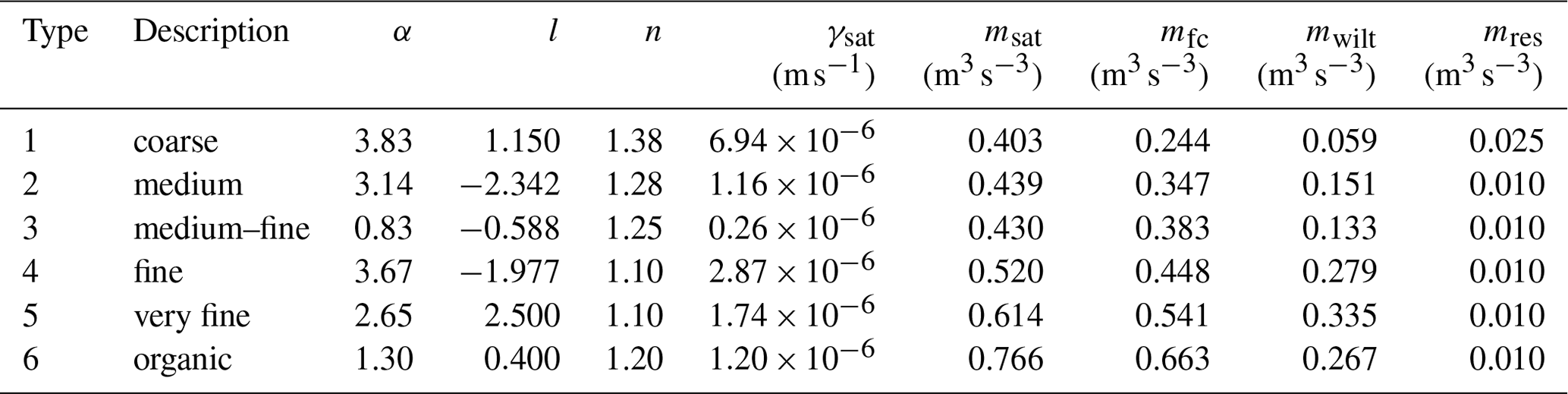
Table 3 Lookup table for albedo parameters.

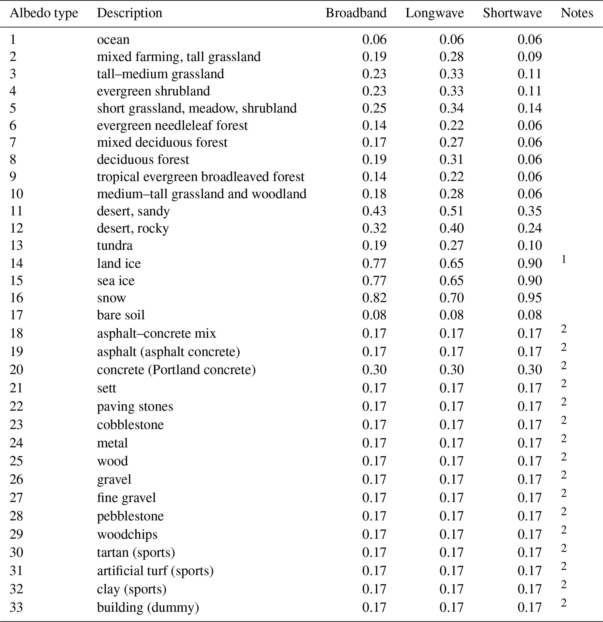
¹ Land ice is treated differently than sea ice. ² Preliminary and/or dummy values.

The root extraction of water from the respective soil layer, S_m,k, is calculated as follows:

$$\begin{array}{}\text{(32)}& S_{\mathrm{m},k}={\displaystyle \frac{L{E}_{\text{veg}}}{{\mathit{\rho }}_{\mathrm{l}}{l}_{\mathrm{v}}}}{\displaystyle \frac{R_{\text{fr},k}}{\mathrm{\Delta }{z}_{\text{soil},k}}}{\displaystyle \frac{m_{\text{soil},k}}{m_{\text{total}}}},\end{array}$$

where m_total is the total water content of the soil,

$$\begin{array}{}\text{(33)}& m_{\text{total}}=\sum _{k=\mathrm{1}}^N{R}_{\text{fr},k}{m}_{\text{soil},k},\end{array}$$

with R_fr,k being the root fraction in soil layer k. Only the layers that have a soil moisture above the wilting point are used in Eq. (33) (i.e., plants are unable to withdraw water from layers with soil moisture below the wilting point). The root distribution within the soil must be chosen such that

$$\begin{array}{}\text{(34)}& \sum _{k=\mathrm{1}}^N{R}_{\text{fr},k}=\mathrm{1}.\end{array}$$

There are two options for the soil moisture bottom boundary condition. The bottom surface can be set to bedrock; i.e., water is not drained. Instead, it is accumulated in the lowest soil layer (water content conservation). Alternatively, the bottom boundary can be set to free drainage, i.e., an open bottom where soil water is continuously lost by drainage (water content is not conserved).

2.2.3 Treatment of pavements

Pavements are treated identically to soil (allowing varying numbers and depths of the pavement layers) but with the physical properties of the pavement material. The pavement layer is impermeable to water, which prohibits the vertical transport of soil moisture. Soil layers are placed below the pavement layers.

2.2.4 Treatment of water bodies

For water surfaces, PALM currently only allows prescription of a bulk water temperature. The energy balance is then solved as for land surfaces but without evapotranspiration from vegetation and bare soil (see above). A skin layer is adopted to calculate the heat flux into the water body, with $C_{\mathrm{0}}=\mathrm{0}\mathrm{J}{\mathrm{m}}^{-\mathrm{2}}{\mathrm{K}}^{-\mathrm{1}}$ and $\mathrm{\Lambda }=\mathrm{1}\times {\mathrm{10}}^{\mathrm{11}}\mathrm{W}{\mathrm{m}}^{\mathrm{2}}{\mathrm{K}}^{-\mathrm{1}}$.

In the case of an ocean surface, a Charnock parameterization can be switched on to account for the effect of waves on the surface friction in terms of a modification of the surface roughness length as described by Beljaars (1994). For details, see Maronga et al. (2020).

2.3 Numerical methods

To solve the energy balance for the surface temperature (T₀), Eq. (1) is first linearized around T₀ at the current time step and then discretized in time using PALM's default Runge–Kutta third-order time-stepping scheme. With this method, an iterative procedure to solve the energy balance is avoided. The prognostic equation then reads

$$\begin{array}{}\text{(35)}& T_{\mathrm{0}}^{t+\mathrm{1}}={\displaystyle \frac{A\mathrm{\Delta }t+C_{\mathrm{0}}{T}_{\mathrm{0}}^t}{C_{\mathrm{0}}+B\mathrm{\Delta }t}},\end{array}$$

where t is the time index and Δt is the current time step. A and B are coefficients given by

$$\begin{array}{ll}\text{(36)}& {\displaystyle }A=& {\displaystyle }{R}_{\mathrm{n}}+\mathrm{3}\mathit{\sigma }{T}_{\mathrm{0}}^{\mathrm{4}}+\left({\displaystyle \frac{\mathit{\rho }{c}_p}{r_{\mathrm{a}}}}\right){\mathit{\theta }}_{\text{mo}}{\displaystyle }& {\displaystyle }+\left({\displaystyle \frac{\mathit{\rho }{l}_{\mathrm{v}}}{r_{\mathrm{a}}+r_{\mathrm{s}}}}\right)\left(q_{\text{mo}}-q_{\text{sat}}+{\displaystyle \frac{\mathrm{d}{q}_{\text{sat}}}{\mathrm{d}T}}{T}_{\mathrm{0}}\right)+\mathrm{\Lambda }{T}_{\text{soil},\mathrm{1}}\end{array}$$

and

$$\begin{array}{}\text{(37)}& B=\mathrm{\Lambda }+\left({\displaystyle \frac{\mathit{\rho }{l}_{\mathrm{v}}}{r_{\mathrm{a}}+r_{\mathrm{s}}}}\right){\displaystyle \frac{\mathrm{d}{q}_{\text{sat}}}{\mathrm{d}T}}+\left({\displaystyle \frac{\mathit{\rho }{c}_p}{r_{\mathrm{a}}\mathrm{\Pi }}}\right)+\mathrm{4}\mathit{\sigma }{T}_{\mathrm{0}}^{\mathrm{3}}.\end{array}$$

Here, $\mathit{\sigma }=\mathrm{5.67037}\times {\mathrm{10}}^{-\mathrm{8}}$ is the Stefan–Boltzmann constant. For vegetated surfaces, where C₀ is zero, Eq. (35) reduces to a diagnostic relationship:

$$\begin{array}{}\text{(38)}& T_{\mathrm{0}}^{t+\mathrm{1}}={\displaystyle \frac{A}{B}}.\end{array}$$

3 CESAR observations

For model evaluation we simulate 2 consecutive clear-sky days observed on 5 and 6 May 2008 at the CESAR site near Cabauw. This period is used because the forcing from the surface was dominant and larger-scale advection is limited. We decided to simulate a 2 d period to study the behavior of the model over a full diurnal cycle and also look at how the first day affects the following day. With a longer period, model drift must be taken care of by, e.g., adding nudging to the forcing and/or data assimilation. This would add additional uncertainty because height-dependent advection, which is needed to drive the LES model, is difficult or impossible to obtain from observations, particularly within the boundary layer where turbulence dominates.

As part of the IMPACT-EUCAARI campaign in May 2008 (Intensive Measurement Period at the Cabauw Tower within the European Integrated project on Aerosol Cloud Climate and Air Quality Interactions; Kulmala et al., 2009), radiosondes were launched daily at 05:00, 10:00, and 16:00 UTC, which we use to initialize the simulations. CESAR features a 213 m high measurement mast with instruments at 1.5, 10, 20, 40, 80, 140, and 200 m (Bosveld, 2020). For our model comparison, we use 10 min averages of temperature, specific humidity, and horizontal wind speed. The measurement accuracy for temperature and humidity is 0.1 K and 3.5 %, respectively (Meijer, 2000). The accuracy for horizontal wind speed is the largest of either 1 % or 0.1 m s⁻¹. Soil temperature is observed at a depth of 0, 2, 4, 6, 8, 12, 20, 30, and 50 cm. The surface soil heat flux is computed from soil heat flux measurements at 5 and 10 cm depths by means of a Fourier extrapolation (see Bosveld, 2020, variable FG0 in their Ch. 19). Net radiation is calculated from the budget of the four radiation components (see Eq. 2). Turbulent fluxes of sensible and latent heat are computed by means of the eddy covariance (EC) method. In the process of calculating EC fluxes from raw turbulence data it is unavoidable that low-frequency contributions to the flux are not represented. For the Cabauw data, the 10 min means are subtracted from the raw turbulent time series; thereafter, a low-frequency correction is applied based on the spectra by Kaimal et al. (1972), with dependence on wind speed and stability (Fred Bosveld, personal communication, 2020). The low-frequency loss correction assumes that all turbulence characteristics follow surface-layer scaling. However, this is not always true. For example, horizontal advection by organized turbulent structures (Eder et al., 2015; De Roo and Mauder, 2018) may add further low-frequency contributions that are not accounted for in the surface-layer scaling. For further information on the instrumentation of the Cabauw site, see Bosveld (2020).

Cabauw is located in the western part of the Netherlands. It is surrounded primarily by meadows with ditches, villages, orchards, and lines of trees. The CESAR tower itself is installed over an area of short grass that is kept at a height of approximately 8 cm. The immediate surroundings of the measuring tower are free of significant heterogeneities for a few hundred meters. During the simulation period from 5 to 6 May 2008 the prevailing wind direction was from the southeast, and the 10 m average wind speed ranged from 2 to 6 m s⁻¹. The convective boundary layer reached a height of approximately 2 km. The groundwater level was 1.3 m in depth. The soil temperature, T_soil, and soil moisture, m_soil, on 5 May 2008 at 05:00 UTC are depicted in Fig. 1 (see Sect. 4). The profiles of temperature θ, humidity q, and horizontal wind v_h retrieved from radiosounding are shown in Fig. 2 together with tower measurements from all available levels (see details in Sect. 5).

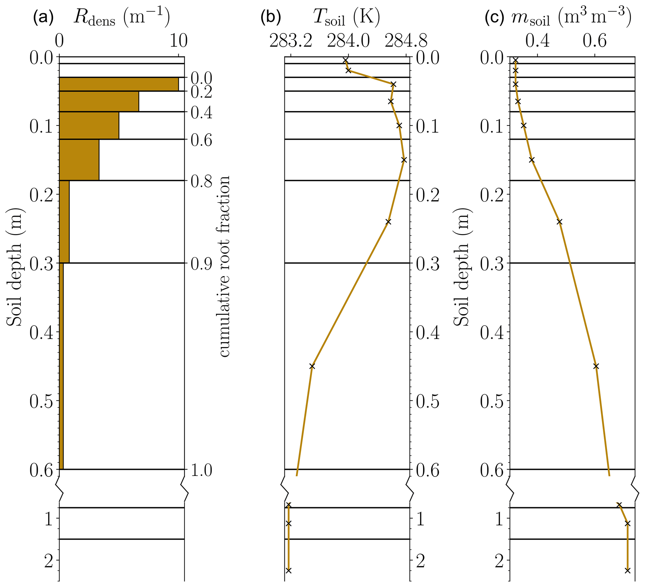
Figure 1 Vertical soil layer setup of root density (R_dens, a) as well as initial profiles of temperature (b) and moisture (c). Note the broken vertical axis with a changed linear increment in the deeper layers. The root fraction of each soil layer (see R_fr in Table 4) is the difference of the cumulative root fraction (Eq. 34; shown on the vertical axis) between two layers.

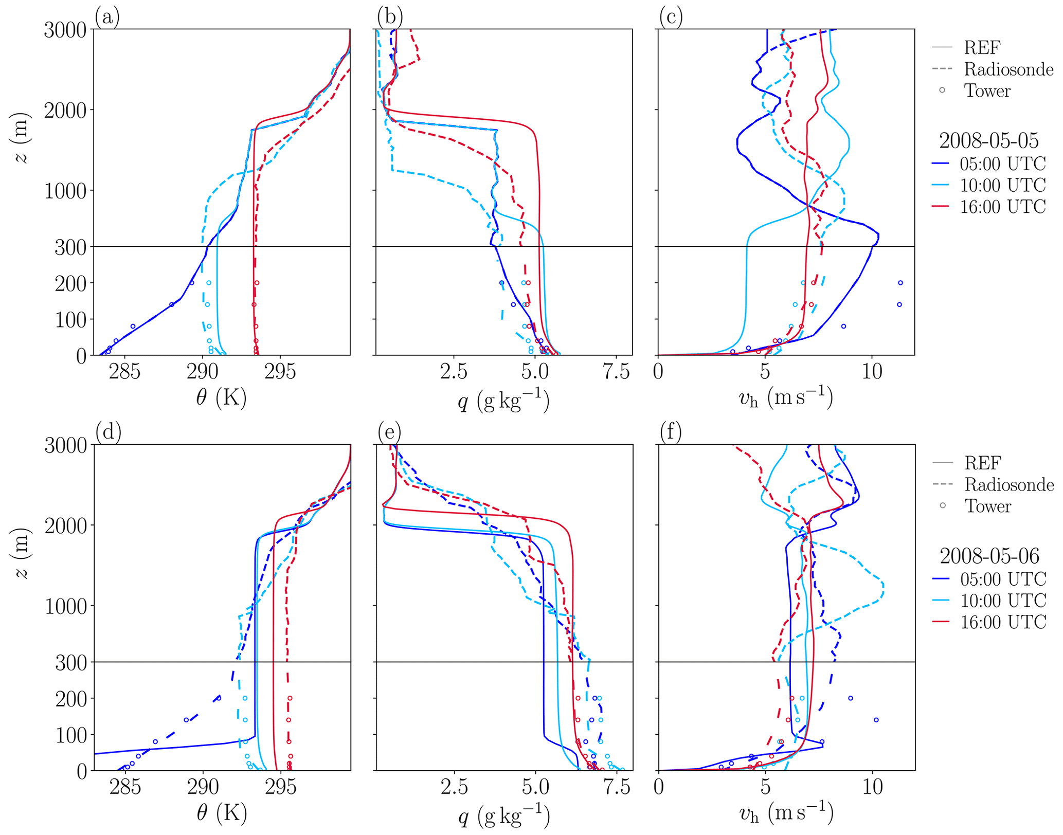
Figure 2 Vertical profiles of θ, q, and v_h measured by radiosonde (dashed lines) and the tower (point markers) at the CESAR site as well as simulated profiles of case REF (continuous lines) during the 2 d period. Note that the lower 300 m is shown with a higher vertical resolution than the layers above to better visualize individual tower measurements (the black horizontal line indicates the break).

4 Simulation setup

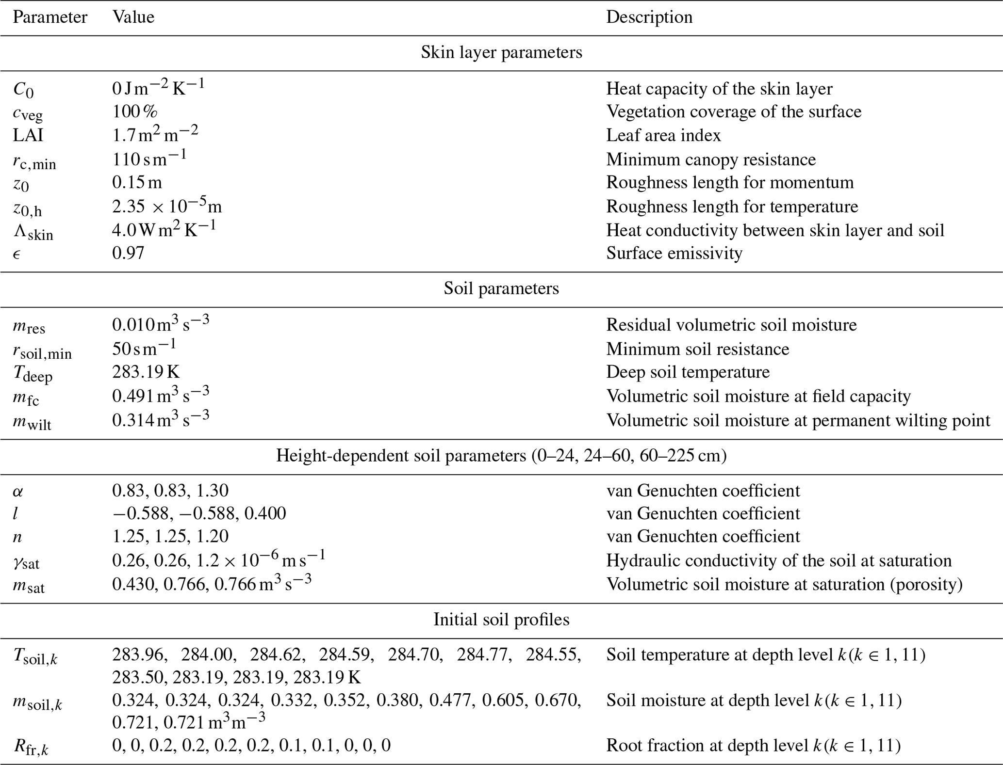
The CESAR site is well-equipped with vegetation and soil information (e.g., Beljaars and Bosveld, 1997), which provides a good opportunity to evaluate the land surface parameterization proposed in the present study. The reference simulation (hereafter referred to as case REF) was set up as a best guess with the Cabauw land surface parameters according to Beljaars and Bosveld (1997), Ek and Holtslag (2004), and Maronga and Bosveld (2017). The vegetation type of the surface is “short grass” with some modifications. The roughness length for momentum is set to 0.15 m, which is representative for a few kilometers of upstream terrain from the Cabauw tower, and the roughness length for temperature is set to $\mathrm{2.35}\times {\mathrm{10}}^{-\mathrm{5}}\mathrm{m}$ (Ek and Holtslag, 2004). The soil layers are defined at depths of 0.005, 0.02, 0.04, 0.065, 0.1, 0.15, 0.24, 0.45, 0.675, 1.125, and 2.25 m. The soil parameters for field capacity and wilting point are 0.491 and 0.314, respectively, which is consistent with a very fine soil texture. The deep soil temperature is fixed at 283.19 K, which is a valid assumption because the lower two soil levels are not reached by diurnal temperature variations (lower part of Fig. 1 does not change over time). The van Genuchten coefficients, the hydraulic conductivity at saturation, and the porosity vary with soil depth. In the uppermost 24 cm, the parameters are set to match medium–fine soil (type 3 in Table 2). The layer between 24 and 60 cm is identical to the uppermost layer except for the porosity, which is increased due to observed large values of soil moisture. Between 60 and 225 cm, the parameters are set to organic soil according to Table 2. In all simulations, the land surface and soil parameters are homogeneous over the model domain. This means that buildings in the small town of Lopik, west of the CESAR tower, are neglected, as are the small ditches that cross the observation site.

The root fraction and initial soil profiles of temperature and moisture are shown in Fig. 1. The root density is based on the study of Jager et al. (1976), who describe the vertical structure as follows. A layer of relatively high root density, R_dens, extends from 3 cm below the surface down to 18 cm, followed by a layer of relatively low root density down to 60 cm of depth. No roots are found near the surface (<3 cm) and in the deep soil layers (>60 cm). The initial soil temperature and moisture profiles are taken from measurement data on 5 May 2008 at 05:00 UTC (shown in Fig. 1). A summary of the land surface scheme configuration is listed in Table 4.

Table 4 Overview of the land surface scheme configuration for case REF.

Case REF is driven by external forcing of incoming shortwave and longwave radiation taken from the Cabauw measurements. The effects of high-altitude aerosols, moisture, and clouds are included in this forcing. Accordingly, the degrees of freedom are reduced and we can focus on parameters of the LSM rather than additional uncertainties of a radiation model. Nonetheless, we performed sensitivity tests using the Rapid Radiation Transfer Model for Global Models (RRTMG; Clough et al., 2005) and a clear-sky radiation parameterization, which are described in detail in Maronga et al. (2020). The longwave outgoing radiation of the surface is calculated from the skin layer temperature using the Stefan–Boltzmann law. The longwave and shortwave albedos for diffusive radiation are set to 0.34 and 0.14, respectively, to fit the dominating grassland. Albedos for direct radiation are calculated according to Briegleb (1992) considering a weak solar zenith angle dependence such that their direct values equal the diffusive ones at 60^∘.

The model domain for case REF is ($x\times y\times z$) $\mathrm{2000}\mathrm{m}\times \mathrm{2000}\mathrm{m}\times \mathrm{4317}\mathrm{m}$ with a horizontal and vertical grid spacing of 50 and 10 m, respectively. A grid sensitivity study is carried out to justify this grid spacing (see Sect. 5). Above the boundary layer (>2000 m), a vertical grid stretching is applied with a stretching factor of 1.08 and a maximum vertical grid spacing of 100 m. Initial profiles of temperature, humidity, and horizontal wind for case REF are taken from radiosounding data and are shown in Fig. 2. The horizontal wind equals the initial u component of the wind vector; i.e., at the beginning of the simulation there is no wind turning with height due to Coriolis force. The geostrophic wind at the top of the domain is set to 7 and 0 m s⁻¹ for the u and v component, respectively. The lateral boundary conditions are cyclic.

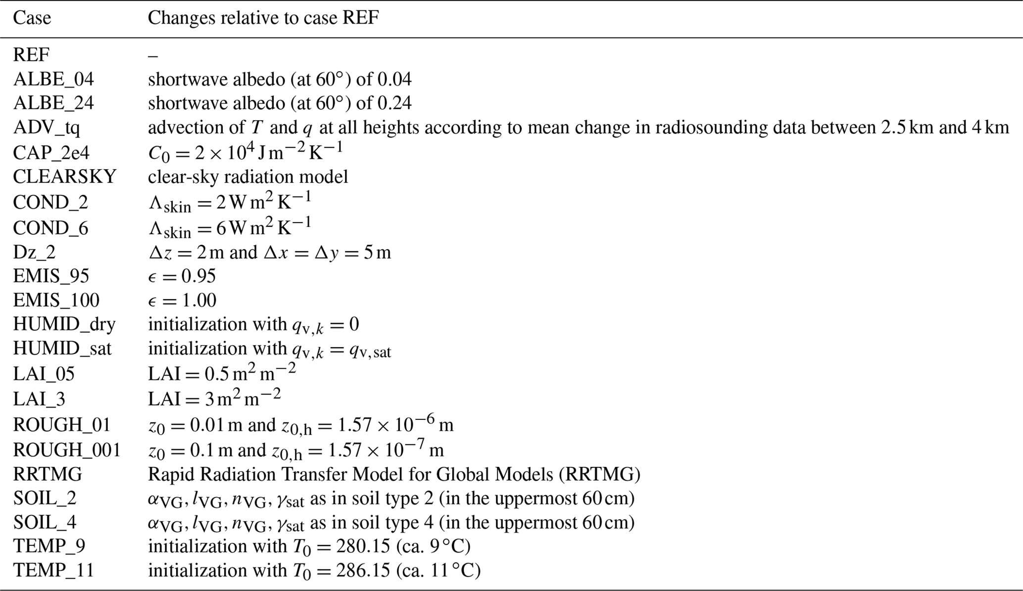
In addition to simulation REF, sensitivity simulations are performed. All sensitivity simulations are based on the reference simulation and only differ by one specific parameter that is varied in a reasonable range. With these sensitivity simulations we do not intend to give a comprehensive parameter study, which usually covers a wide range of parameters. Nonetheless, the simulations provide an idea of how sensitively the model reacts to specific parameters or processes included. This is mainly motivated by the fact that in many simulation setups the respective input data for the land surface parameters are often not available or only roughly available, imposing rather high uncertainty on these data. An overview of the sensitivity simulations and their well-defined change compared to case REF is given in Table 5.

Table 5 Overview of the case study and changes relative to case REF.

5 Results

5.1 Boundary-layer profiles

At first, we will look at the vertical profiles of the radiosonde and tower measurements. Figure 2 shows vertical profiles of θ, q, and v_h, indicating the evolution of the boundary layer during the considered period of time in Cabauw at the times of the radiosonde ascents. Both nights show a stable nocturnal boundary layer before sunrise (at 05:00 UTC). A nighttime low-level jet is observed in the horizontal wind. Profiles of potential temperature and water vapor mixing ratio show a well-mixed convective boundary layer at 10:00 and 16:00 UTC on both days. Over the course of the 2 d, the depth of the convective boundary layer increases. The profiles of v_h show a mismatch between the radiosounding measurements and the tower data. This is explained by different analysis timescales. The radiosonde records instantaneous values with a sampling frequency of 0.1 Hz, which results in five recording heights below 300 m. Conversely, data from the cup anemometers at the mast are temporally averaged over 10 min based on a 3 s running mean calculated with an update frequency of 4 Hz (Bosveld, 2020). Thus, the mean tower profiles can be overestimated or underestimated by the instantaneous values of the radiosonde. Note that we initialize the simulations with data from the radiosonde ascent because it reaches high enough, but comparisons are made against tower data due to the higher temporal resolution.

Figure 2 also shows the vertical profiles of the reference simulation, which are temporally averaged over 15 min and horizontally averaged over the whole domain. A comparison of observed profiles of θ and q with those of the LES show that the boundary-layer depth is underestimated by the simulation at 10:00 UTC on the first day. One hypothesis to explain this is that the turbulence development during model spin-up, i.e., on the first morning, takes longer than in reality. The horizontal wind speeds of the model and observations do not agree at 10:00 UTC on the first day. At 16:00 UTC on the first day, the simulation slightly overestimates the boundary-layer depth despite fairly good agreement of the model and observations regarding mixed-layer temperature and humidity values. The wind profiles agree well with observations. At night (6 May 2008, 05:00 UTC), the near-surface temperature is significantly lower (out of range at ca. 281 K) than measured. Similar to the mixing layer, the simulation also underestimates the nocturnal boundary-layer depth. At the same time, the near-surface humidity shows small differences between the model and reality. The simulated horizontal wind speed also depicts a low-level jet, but compared with observations it occurs closer to the surface, in accordance with the simulated nocturnal boundary-layer depth. Even though the LES cannot reproduce the nocturnal observations precisely, the mixed layer quickly develops the next morning (6 May 2008, 10:00 UTC), which is in agreement with findings of van Stratum and Stevens (2015). At 10:00 UTC on the second day, the simulation indicates a warmer and deeper boundary layer compared to the observations, which could be caused by advection processes in reality modifying the residual layer and thus the boundary-layer evolution during the morning transition. The wind profiles agree fairly well with observations. The temperature profile on 6 May 2008 at 16:00 UTC shows that the simulation underestimates the mixed-layer temperature but overestimates the depth of the boundary layer. This overestimation suggests that the total energy input into the boundary layer is similar to the observations but distributed over a deeper layer. The humidity profiles agree well with observations in the lowest 1000 m but deviate above this height in accordance with the differences in boundary-layer depth. The horizontal wind is slightly overestimated at 16:00 UTC on the second day. In general, the simulated profiles are much more constant with height in the well-mixed layer because they depict domain averages as opposed to local measurements, so a direct comparison is inherently improper. Above the boundary layer in the free atmosphere, synoptic-scale processes dominate in reality. Because we did not consider these processes in our simulations, profiles may deviate. Given that the surface forcing in this particular case was the dominant forcing for the development of the boundary layer, this deficiency should not compromise the present evaluation study.

5.2 Evaluation of energy balance components

5.2.1 Net radiation

Figure 3 shows the time series of surface net radiation, which follows a diurnal cycle typical for clear-sky conditions. At noon, the reference simulation underestimates R_n, whereas it overestimates R_n at night; i.e., it is less negative by approximately 30 W m⁻². The nocturnal differences are due to much lower surface temperatures of 280 K in case REF vs. 285 K in the observations (not shown). The reason for this is that the longwave outgoing radiation flux is underestimated because the incoming radiation in case REF is prescribed. At around 12:00 UTC on the second day, clouds influence the net radiation, which is indicated by fluctuations in the curve. Because case REF is driven with SW_↓ taken from CESAR data, this cloud effect on the surface net radiation is included and can also be seen in the other surface fluxes (see Figs. 4, 5, and 6). The maximum and minimum values of net radiation for case REF indicate low horizontal variation of approximately $\pm \mathrm{10}\mathrm{W}{\mathrm{m}}^{-\mathrm{2}}$ at noon. Figure 3 also depicts the effect of different land surface properties and simulation setups on the surface radiation. At this point we want to emphasize again that the discussion of the sensitivity simulations is not intended to find the perfect parameter combination but to give an estimate of the sensitivity of the modeled energy balance components on specific land surface parameters and outline their complex interactions among each other. Note that we will only highlight the cases that lead to the largest differences compared to case REF for the respective variable. In Fig. 3, these are mostly the changes to the albedo and the radiation models, as well as cases LAI_05 and HUMID_sat, which have the largest impact on the surface net radiation. The most obvious differences occur in the albedo sensitivity simulations. An increase in the albedo (case ALBE_24) decreases R_n and vice versa (case ALBE_04), with maximum deviation from case REF of approximately $\pm \mathrm{100}\mathrm{W}{\mathrm{m}}^{-\mathrm{2}}$ at noon. This deviation suggests that mismatches in the estimated albedo cause significant errors in the surface net radiation during daytime. However, the spread of the non-highlighted simulations (gray) is approximately 50 W m⁻² at noon. This spread implies that variations in the surface parameters (e.g., emissivity, roughness length) also significantly affect the surface net radiation. Besides this, cases EMIS_95, EMIS_100, ROUGH_01, ROUGH_001, SOIL_2, and SOIL_4 are always among the non-highlighted cases in Figs. 4, 5, and 6. With RRTMG, radiative fluxes are calculated for each horizontal grid box of the LES based on time, geographical location, air pressure, and local profiles of temperature and humidity (Clough et al., 2005) instead of being taken from measurements. A key feature of the RRTMG is the direct cooling of air due to longwave radiative flux divergence, particularly during nighttime. This results in cooling rates on the order of 0.1 to 0.3 K h⁻¹ (see, e.g., Maronga and Bosveld, 2017, their Fig. 1). This effect is not included in case REF, wherein incoming radiation is prescribed, and in case CLEARSKY. In case RRTMG, the simulated R_n approaches that of the observations during day and night, though it slightly underestimates the surface net radiation at noon by approximately 30 W m⁻². Note that we use default input of the RRTMG with standard profiles of water vapor, other trace gases, and aerosol concentration above the model top, which does not necessarily reflect the real conditions at Cabauw during the simulated time period and may impact the simulated surface net radiation as well. The clear-sky model simulates R_n more accurately during the day but also marginally overestimates net radiation during the night by 10 to 20 W m⁻². Case LAI_05 has a smaller R_n than case REF because a smaller LAI significantly decreases LE and increases H, which leads to higher surface temperatures during the day. Higher temperatures result in higher LW_↑. In the case of a saturated humidity mixing ratio (case HUMID_sat), the surface temperature is higher during both day and night due to significant alterations to LE, H, and G. This higher surface temperature again leads to higher LW_↑ and hence lower R_n. Except for ALBE_04, the simulations tend to underestimate the surface net radiation during daytime, while the simulated surface net radiation tends to overestimate the observed surface net radiation during the night.

Figure 3 Time series of surface net radiation R_n as measured at Cabauw (OBS) and domain-averaged R_n for all simulated cases listed in Table 5. Only case REF and some relevant cases are highlighted; all others are shown in gray. The gray transparent area shows minimum and maximum values of the net radiation for case REF based on instantaneous hourly horizontal cross sections.

Figure 4 Time series of surface sensible heat flux H as measured at Cabauw (OBS) and domain-averaged H for all simulated cases listed in Table 5. Only case REF and some relevant cases are highlighted; all others are shown in gray. The gray transparent area shows minimum and maximum values of the sensible heat flux for case REF based on instantaneous hourly horizontal cross sections.

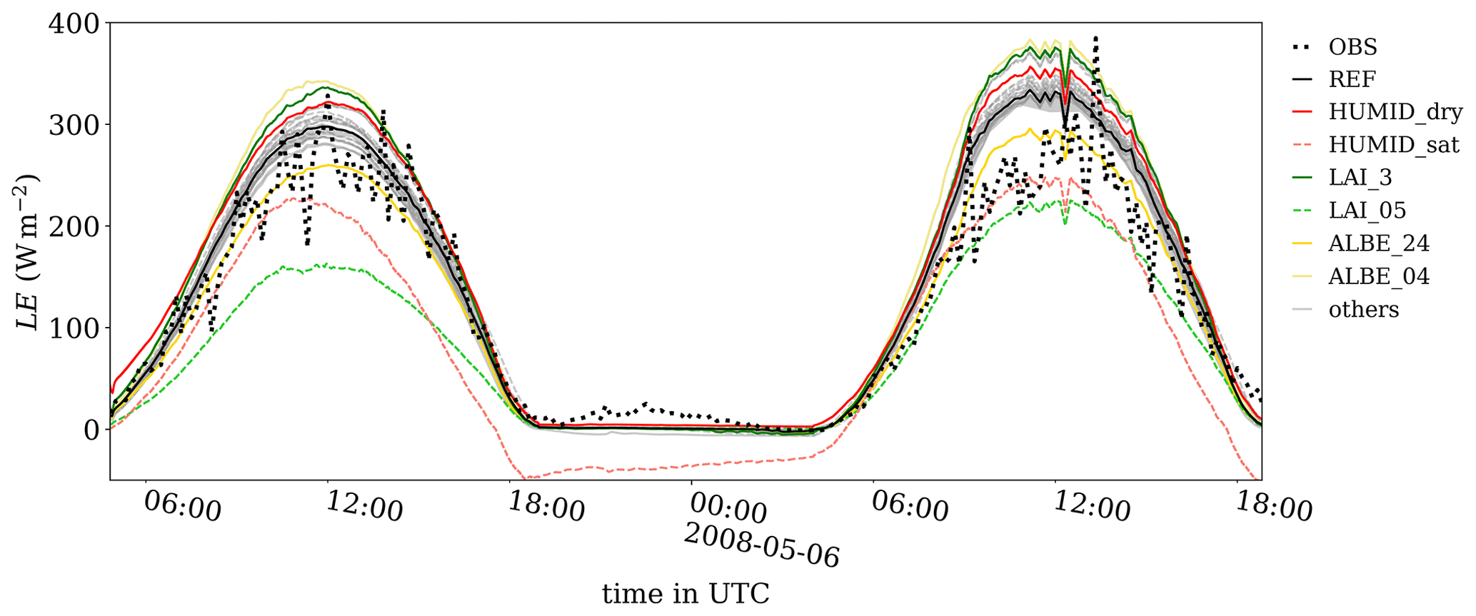
Figure 5 Time series of latent heat flux LE as measured at Cabauw (OBS) and domain-averaged LE for all simulated cases listed in Table 5. Only case REF and some relevant cases are highlighted; all others are shown in gray. The gray transparent area shows minimum and maximum values of the latent heat flux for case REF based on instantaneous hourly horizontal cross sections.

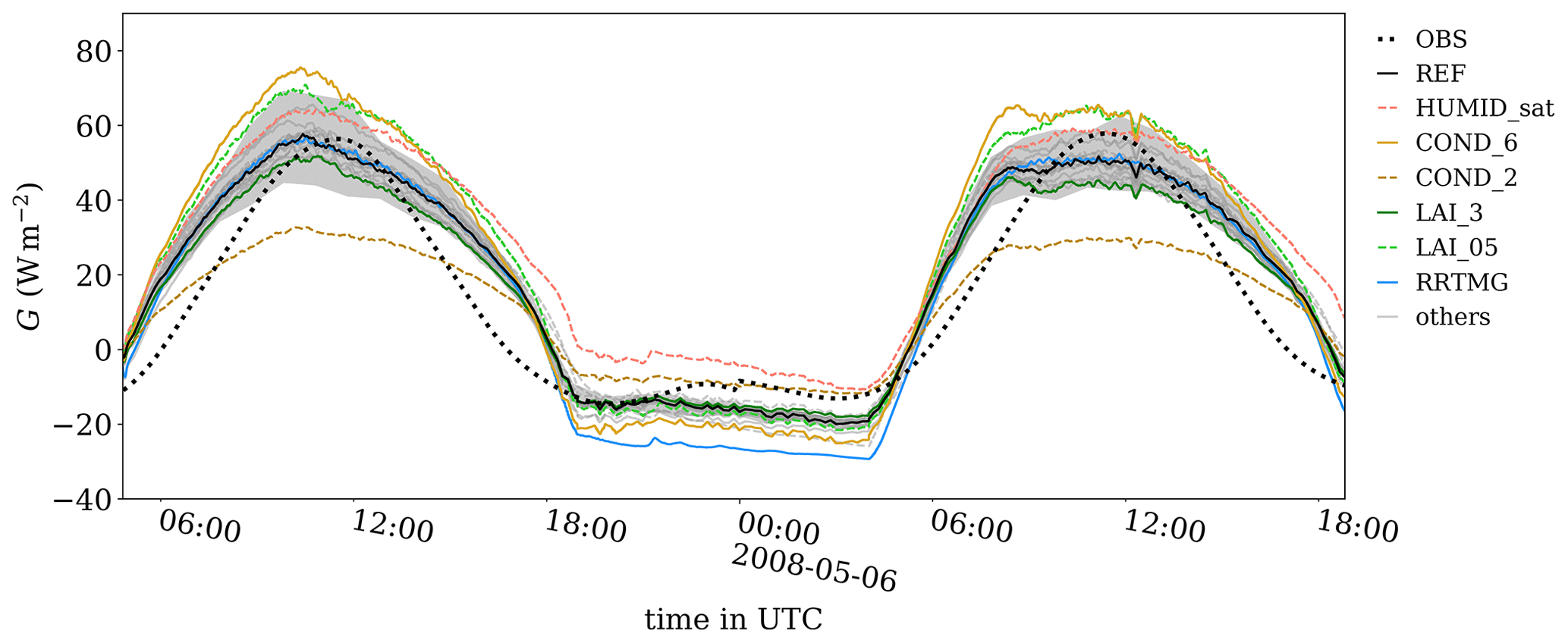
Figure 6 Time series of ground heat flux G as measured at Cabauw (OBS) and domain-averaged G for all simulated cases listed in Table 5. Only case REF and some relevant cases are highlighted; all others are shown in gray. The gray transparent area shows minimum and maximum values of the ground heat flux for case REF based on instantaneous hourly horizontal cross sections.

5.2.2 Sensible heat flux

Figure 4 shows that the observed surface sensible heat flux reaches a maximum of approximately 100 and a minimum of $-\mathrm{50}\mathrm{W}{\mathrm{m}}^{-\mathrm{2}}$. Compared to observations (OBS), case REF significantly overestimates H by up to approximately 40 W m⁻², with the largest overestimation at noon. Moreover, the model overestimates H in the morning and afternoon hours; it is positive earlier and later, respectively. At night, case REF shows a constantly increasing H from −25 to $-\mathrm{15}\mathrm{W}{\mathrm{m}}^{-\mathrm{2}}$, whereas the observations show a secondary minimum of ca. $-\mathrm{50}\mathrm{W}{\mathrm{m}}^{-\mathrm{2}}$ between 20:00 and 23:00 UTC. Here, we note that the depicted sensible heat fluxes from the simulations are domain-averaged values. Considered locally in the simulation, we can detect similar temporal fluctuations in H, though with a smaller amplitude than those observed at the CESAR site. The horizontal variation (maximum and minimum values) of the sensible heat flux of case REF is approximately $\pm \mathrm{30}\mathrm{W}{\mathrm{m}}^{-\mathrm{2}}$ at noon. Like case REF, all sensitivity simulations tend to overestimate the observed heat flux, and the spread among the considered cases is significant. At noon, when the spread among all simulations is largest, differences in simulated heat fluxes approach 120 W m⁻². ALBE_24, LAI_3, and HUMID_dry show the best agreement with the observations. With a higher albedo (ALBE_24), the available energy at the surface is lower (see Fig. 3). The lower available surface energy results in smaller fluxes of H and LE. Besides changing the albedo, cases LAI_3 and LAI_05 show the largest impact on H because with lower and higher LAI the available energy is preferentially partitioned into H and LE, respectively. Similarly, the available energy is also preferentially partitioned into H and LE for humid and dry air, indicated by HUMID_sat and HUMID_dry, respectively.

5.2.3 Latent heat flux

Figure 5 shows time series of the latent heat flux. The observations range from 0 W m⁻² during the night to approximately 300 W m⁻² at noon. Case REF matches the observation reasonably well during daytime and nighttime, even though it overestimates LE during the second day. The maximum and minimum values of latent heat flux for case REF indicate low horizontal variation of approximately $\pm \mathrm{10}\mathrm{W}{\mathrm{m}}^{-\mathrm{2}}$ at noon. Having a lower LE than case REF, ALBE_24 best matches the observed LE of the second day. Additionally, case LAI_05 significantly underestimates LE by preferentially partitioning the available energy into H (Fig. 4). Moreover, case HUMID_sat stands out because it shows a negative LE during night due to dew formation in the model. Observations suggest that dew formation was not observed in Cabauw because there is no negative LE. The maximum spread of all non-highlighted sensitivity studies is approximately 50 W m⁻². This spread is up to 170 W m⁻² for the highlighted sensitivity studies. From Fig. 4 and Fig. 5 we calculate the daytime Bowen ratio ${\mathit{\beta }}_{\mathrm{0}}=\frac{H}{LE}$ (not shown). We find that the difference between the Bowen ratio of the simulations and that observed at Cabauw (${\mathit{\beta }}_{\mathrm{0},\text{sim}}-{\mathit{\beta }}_{\mathrm{0},\text{obs}}$) ranges from −0.1 to +0.2, except for cases HUMID_sat and LAI_05, which have significantly higher Bowen ratios compared to observations. As opposed to other models, which were shown to systematically overestimate the Bowen ratio measured in Cabauw during summer (Schulz et al., 1998; Sheppard and Wild, 2002), we cannot identify a systematic bias for the Bowen ratio of PALM's LSM by means of the analyzed period.

Taking into account that modeled surface net radiation is underestimated but the observed modeled latent and sensible fluxes both exceed the observed values, while the modeled Bowen ratio matches the observed values, one can conclude that the remaining energy is included in the ground heat flux, which will be discussed in the next paragraph.

5.2.4 Ground heat flux

Figure 6 shows the time series of the ground heat flux, which reaches 60 W m⁻² during daytime in the observations. With respect to the amplitude of G, case REF shows good agreement with the observation. However, the shape of the time series is discernibly different. During daytime, OBS has a pseudo-sinusoidal shape, whereas the simulations have a more humped-shaped diurnal variation. We attribute this to the method used to derive the observed ground heat flux, which involves the average soil heat flux at 10 and 5 cm depths (details in Sect. 3). In the model, the ground heat flux is parameterized according to Eq. (6), and thus only the temperature gradient between the surface and 0.5 cm is accounted for. Hence, the simulated G resembles the diurnal cycle of the surface temperature, while the observed G correlates with the soil temperature. Observations and case REF agree well at noon, with values of G around 55 W m⁻², whereas in the afternoon at 15:00 UTC case REF is almost 10 W m⁻² higher than the observations. The horizontal variation (maximum and minimum values) of the ground heat flux for case REF is approximately $\pm \mathrm{10}\mathrm{W}{\mathrm{m}}^{-\mathrm{2}}$ at noon. Remarkably, all simulations have a fairly small spread at this time. During the day, changing the heat conductivity between the skin layer and uppermost soil layer has the largest impact on the ground heat flux, with smaller and larger G observed in cases COND_2 and COND_6, respectively. This can be attributed to the linear relationship between G and Λ in Eq. (6). Also, the LAI sensitivity cases show a relatively large deviation from case REF at noon, with increased (decreased) G for LAI_05 (LAI_3). At noon, the spread among all simulations is approximately 40 W m⁻², whereas the non-highlighted cases show a maximum deviation from REF of no more than $\pm \mathrm{10}\mathrm{W}{\mathrm{m}}^{-\mathrm{2}}$. In the night, cases HUMID_sat and RRTMG stand out. In both cases the controlling variable is the (near-)surface temperature (see Fig. 9). In case RRTMG, the surface cools, while the soil temperature does not change by the same amount (see Fig. 8), which leads to a strong ground heat flux directed towards the surface. In case HUMID_sat, the surface remains relatively warm, which results in a small negative G. Except for cases HUMID_sat and COND_2, the model tends to simulate a stronger upward-directed ground heat flux at night compared to the observations. Compared to the observations, case COND_2 overestimates G during the night, whereas it underestimates G at noon, which points to a stability dependence of the conductivity Λ. Even though this is technically realized in the code, the standard values for short grass do not differ between stable and unstable conditions due to a lack of knowledge of the correct relationship between Λ and stability. As cases COND_2 and COND_6 do not have a significant impact on any of the other variables, we can infer that uncertainties in modeling G are relatively small. Nonetheless, note that we only analyzed a short period of 2 d. For longer simulation times covering multiple days, e.g., for heat-wave scenarios wherein heat storage within the soil becomes important, it might become relevant to accurately simulate G. Furthermore, the ground heat flux is small compared to the surface net radiation as well as the surface sensible and latent heat fluxes.

As the modeled and observed ground heat fluxes are in a similar range but the modeled surface net radiation underestimates the observed values, the available energy in the simulation is smaller compared to the observation. However, at the same time, the modeled fluxes, into which the available energy is partitioned, exceed the observed values. One possible explanation for this discrepancy could be mismatches coming with the observed values of the energy balance components, which will be discussed in the next paragraph.

5.2.5 Uncertainty in model–observation comparison due to energy balance non-closure

At this point we want to briefly address the well-known problem of energy balance non-closure and how this affects our model–observation comparison. Similar to many other sites, eddy covariance measurements at the Cabauw site suffer from energy balance non-closure (de Roode et al., 2010). To date, the leading hypothesis is that low-frequency contributions are inherently not captured by the eddy covariance method, leading to the situation that the sum of the surface heat fluxes underestimates the available energy by 10 % to 30 % (Foken et al., 2011). Figure 7 shows the residual of the energy balance in the observations (RES) and the particular differences between the simulated reference case REF and the observed energy balance components. Note that the energy balance in our simulations is closed (according to Eq. 1) with $C_{\mathrm{0}}=\mathrm{0}\mathrm{J}{\mathrm{m}}^{-\mathrm{2}}{\mathrm{K}}^{-\mathrm{1}}$ (i.e., no storage), and thus no residual for the simulations is shown. The residual in the observation exhibits a diurnal cycle with only small positive values of approximately 15 W m⁻² during nighttime, while during daytime the residual indicates that up to 150 W m⁻² is missing in order to close the surface energy balance. The differences between the simulated and observed H and LE correlate negatively with the residual. This suggests that either the model overestimates H and LE, or, conversely, the observations underestimate H and LE due to low-frequency losses in the EC method. Figure 7 thus emphasizes the uncertainty inherent in such a model–observation comparison, especially during daytime. In this respect, we summarize the four components of the energy balance as represented reasonably well by the LES–LSM interface.

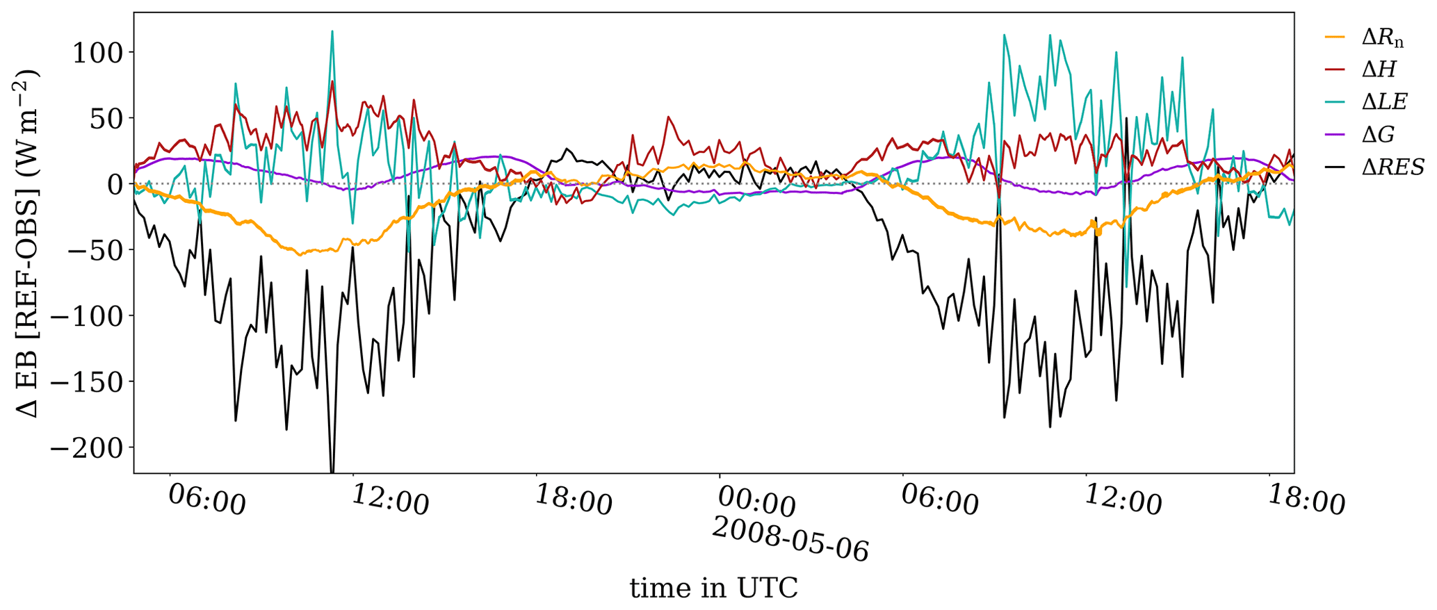
Figure 7 Time series of the individual differences between case REF and observations for the energy balance components R_n, H, LE, and G, as well as the residual $\text{RES}=R_{\mathrm{n}}-H-LE-G$ from the Cabauw observations.

Figure 8 Vertical profiles of soil temperature as measured at Cabauw (OBS) and domain-averaged soil temperature for all simulated cases listed in Table 5. Only case REF and some relevant cases are highlighted; all others are shown in gray.

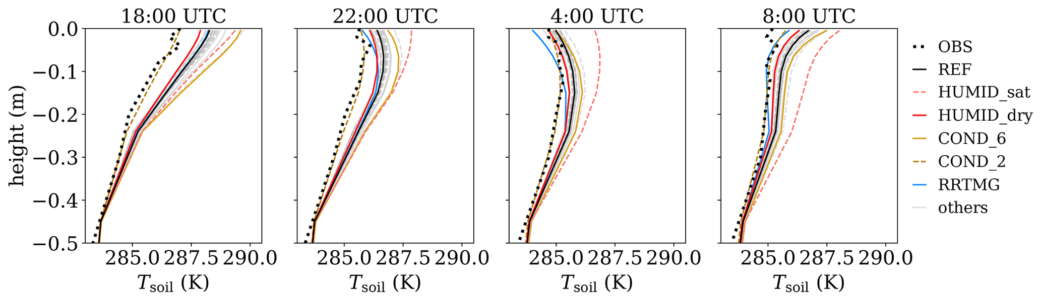
5.3 Soil temperature

Figure 8 shows mean profiles of soil temperature, T_soil, averaged over the whole domain and over 15 min. Note that there are doubts about the quality of the CESAR soil temperature observations because of problems during calibration (Bosveld, 2020) and the speculation that the sensors sunk deeper into the soil over time (Fred Bosveld, personal communication, 2020). Hence, observations are not a reliable reference to evaluate the model. Nevertheless, we discuss the variation among the different simulations. In the late afternoon of the first day (18:00 UTC), case REF shows a continuous decrease with depth from 288 K close to the surface to 283.5 K at −50 cm. During the night, the soil begins to cool down starting at the surface, where it reaches 285 K at 04:00 UTC. The maximum soil temperature occurs at a depth of −15 cm. The near-surface soil temperature responds quickly to positive net radiation (at 08:00 UTC) such that the maximum temperature is again close to the surface. The parameters with the largest spread – up to 4 K during the day and 2 K during the night – are, like for G, the conductivity and atmospheric humidity. The non-highlighted cases have a spread of approximately 1 K. This spread indicates that, e.g., changing radiation or vegetation parameters has only minor effect on the soil temperature. A higher conductivity (COND_6) results in higher soil temperatures, especially in the late afternoon (18:00 UTC), because the heat of the surface net radiation is more easily conducted into the soil (see Fig. 6); correspondingly, COND_2 has smaller T_soil. During the night, the lower atmosphere in case HUMID_sat cools less rapidly than case REF (see Fig. 9); therefore, the soil remains relatively warm, too.

5.4 Evaluation of atmospheric quantities

In this section, we evaluate the quantities characterizing the lower atmosphere: temperature, humidity, and wind speed. First, we discuss the nighttime situation followed by the daytime situation. Then, we discuss the results of the sensitivity study.

5.4.1 Stability of the nocturnal boundary layer

Figure 9 shows the vertical profiles of potential temperature during the night. At 18:00 UTC, the lowest levels start to cool, while the upper levels remain in a vertically well-mixed state; observations and case REF agree well. At 22:00 UTC, the stable boundary layer of case REF reaches a height of approximately 75 m and has a mean potential temperature gradient of 0.1 K m⁻¹. Tower measurements, however, suggests the atmosphere is less stable (0.02 K m⁻¹) and the stable layer is at least 200 m deep (not shown). Above the mast we have no data to compare the simulated temperature profile with. The radiosounding profiles at 05:00 UTC in Fig. 2 show that there is no residual layer, but the stable layer extends up to the capping inversion at approximately z=1800 m. The next morning at 08:00 UTC, observations show an already vertically well-mixed lower boundary layer, while in the simulations a stable layer at approximately 100 m is still present and gets eroded due to surface heating and mixing processes. This is consistent with Fig. 11, which indicates a faster temperature increase at z=40 m compared to the observations.

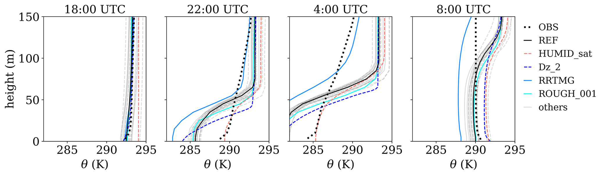
Figure 9 Vertical profiles of mean potential temperature as measured at Cabauw (OBS) and for all cases listed in Table 5. Only case REF and some relevant cases are highlighted; all others are shown in gray.

The misrepresentation of the nocturnal boundary layer is a common issue for atmospheric models (see, e.g., van Stratum and Stevens, 2015). Due to the smaller turbulence scales at nighttime than at daytime, a smaller grid spacing is usually required to resolve the dominant turbulent eddies. Thus, we suspect that the grid spacing of case REF might be too coarse. However, compared to case REF, case Dz_2, with smaller grid spacing, is even more stable during the night hours. The case with smaller grid spacing has a lower boundary-layer depth and cooler near-surface temperature than case REF, in agreement with van Stratum and Stevens (2015). These results suggest that the coarse resolution might not explain the misrepresentation of the stable boundary layer, though. With only one grid sensitivity simulation, a nonlinear relationship cannot be fully ruled out. For more information on grid spacing of models in stable conditions, see Sullivan et al. (2016) and Dai et al. (2021). Another parameter affecting the diffusivity is the subgrid-scale scheme of the LES. Yet, the subgrid-scale scheme of Dai et al. (2021), which is more diffusive in the middle of the stable boundary layer but less diffusive towards the surface, does not change the stability of the simulation (not shown). Alternatively, overly low diffusivity could be due to low wind speed; however, the simulated wind speed in Fig. 13 agrees well with observations. Note that as LW_↓ is prescribed in case REF, we can exclude all factors affecting the longwave incoming radiation, e.g., humidity or clouds, as possible reasons for the misrepresentation of the nighttime stable layer. At 02:00 UTC, case RRMTG, wherein cooling of the air column by vertical divergence of radiative fluxes is directly considered, reveals an even cooler and more stable (compared to REF) nighttime boundary layer. Too much cooling indicates overly low humidity in the atmosphere, which is in agreement with Fig. 12, where humidity is slightly smaller in case RRMTG than the observations between 00:00 and 06:00 UTC. Furthermore, compared to the observations, the simulations indicate a less negative H (see Fig. 4), though we note that the simulated H is a domain-averaged value, while the observed value is taken from a point measurement with more temporal fluctuation. Nevertheless, according to the less negative H, the near-surface layer should be less stable in the simulations. This is not the case (see profiles from Fig. 11). It is unclear why the nocturnal boundary layer is misrepresented in the LES.

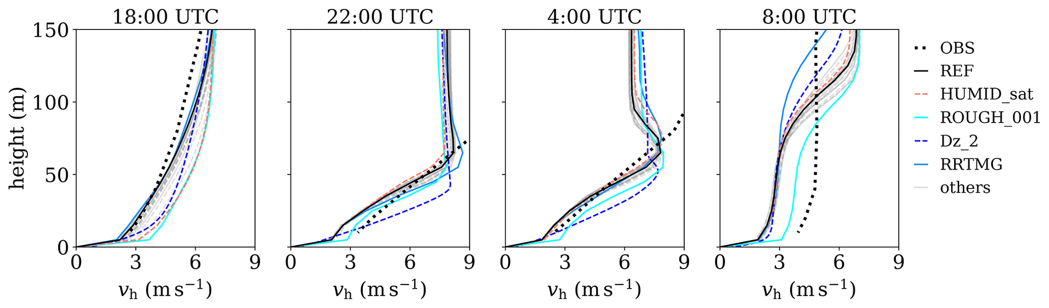
Figure 10 Vertical profiles of mean horizontal wind speed as measured at Cabauw (OBS) and for all cases listed in Table 5. Only case REF and some relevant cases are highlighted; all others are shown in gray.

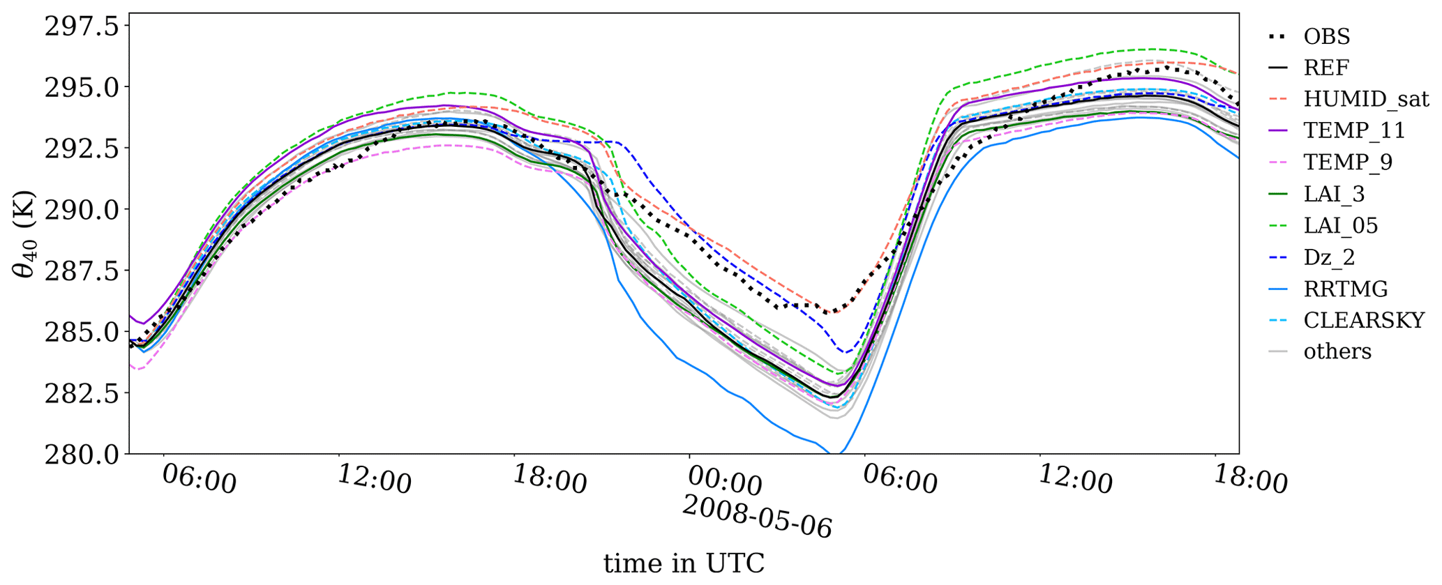
Figure 11 Time series of mean potential temperature at 40 m as measured at Cabauw (OBS) and for all cases listed in Table 5. Only case REF and some relevant cases are highlighted; all others are shown in gray.

Figure 12 Time series of mean total water mixing ratio at 40 m as measured at Cabauw (OBS) and for all cases listed in Table 5. Only case REF and some relevant cases are highlighted; all others are shown in gray.

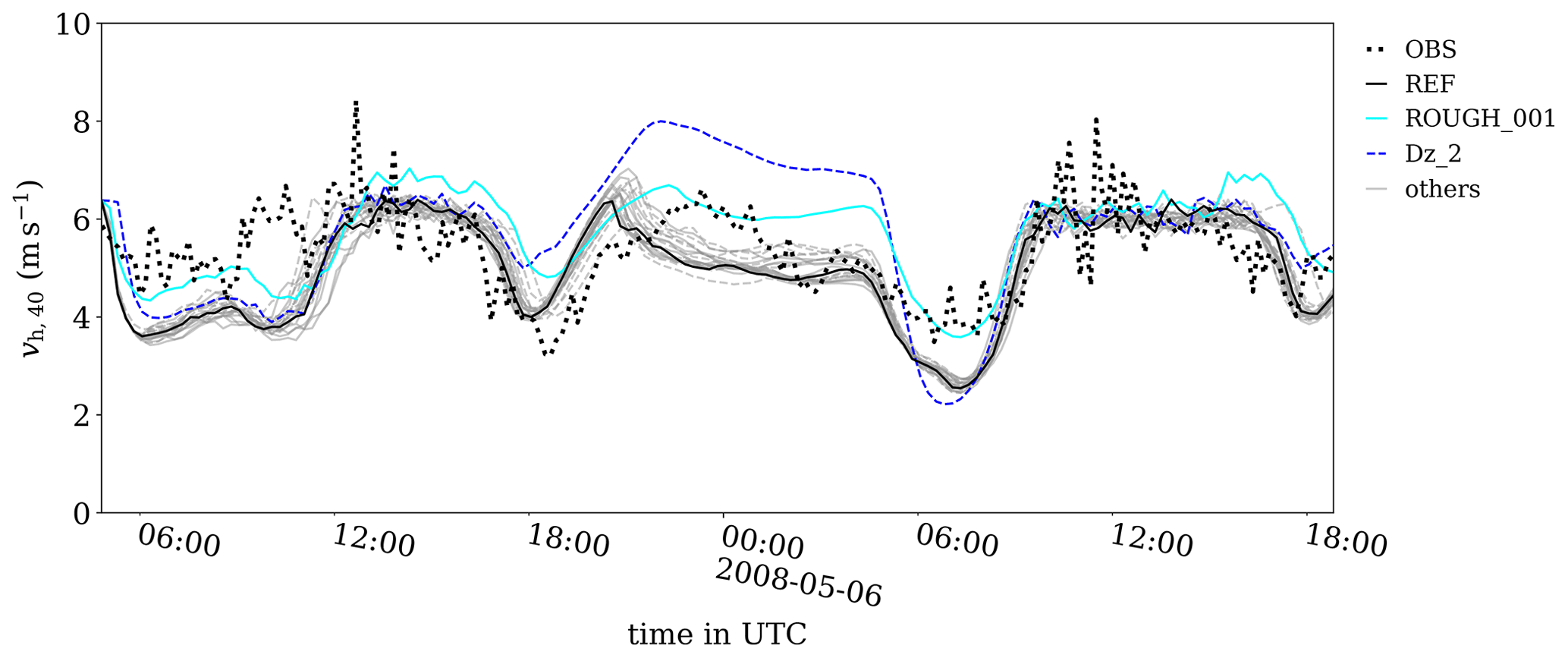
Figure 13 Time series of mean horizontal wind speed at 40 m as measured at Cabauw (OBS) and for all cases listed in Table 5. Only case REF and some relevant cases are highlighted; all others are shown in gray.

Figure 10 shows vertical profiles of horizontal wind speed v_h. Again, we find that case REF and all sensitivity studies simulate a shallower nocturnal boundary layer than observed at the CESAR tower (22:00 and 04:00 UTC). A low-level jet develops in reality and in the simulations. According to the radiosounding measurements on 6 May 2008 at 05:00 UTC (Fig. 2), the maximum wind speed occurs at approximately 500 m. In the LES (case REF), however, the low-level jet has a maximum velocity between a height of 60 and 70 m (see Figs. 2 and 10). In the morning, when convective mixing sets in, the wind profiles become more well-mixed. At 08:00 UTC, we already find a mixed layer in reality. By contrast, the stable layer has not been fully eroded in the LES. Therefore, the wind speed in the residual layer (above ca. 100 m) is still higher than that of the lower 100 m. Even though case RRTMG shows a large influence on the whole temperature profile (Fig. 9), the wind profile only deviates from case REF above the low-level jet and during the morning transition when the stable layer is already further eroded. Likewise, case HUMID_sat does not deviate much from case REF (see Fig. 10). Conversely, case ROUGH_001 deviates significantly from case REF in the wind profiles but does not show significant changes in the temperature profiles (Fig. 9). Only case Dz_2 shows a strong interconnection between temperature and wind profiles.

5.4.2 Potential temperature

The CESAR tower samples temperature, humidity, and horizontal wind speed at 10, 40, and 80 m heights (wind speed is not available at 1.5 m). We compare time series of the 40 m level because 10 m lies between the first and second grid level and 80 m is likely above the nocturnal boundary layer (see discussion of Fig. 9). Figure 11 shows the diurnal cycle of temperature at z=40 m, which, at first sight, agrees fairly well between observations and case REF. The temperature amplitude is around 10 K, and peak temperatures reach 295 and 296 K between 16:00 and 17:00 UTC on the first and second day, respectively. Significant differences exist during the night and during the second day: during the night, the temperature at 40 m of height for case REF is lower than the observations. Hence, the simulated boundary layer is more stable than the observations (see Fig. 9), as discussed earlier. The following morning, the boundary layer warms quickly between approximately 06:00 and 08:00 UTC in the simulation, whereas in reality the temperature increases more slowly. Again, the reason is that the model develops a much shallower stable boundary layer (with a residual layer above; see Fig. 2) than the observations. Once the surface heating in the morning has eroded the stable layer up to 40 m, the temperature increases rapidly at that level as it is heated from the surface and from above, where warmer air from the residual layer is mixed into the shallow layer. In reality, where the stable layer is much deeper, the air at 40 m of height is only heated from the surface and not by entrainment. The sensitivity study shows that during the night case HUMID_sat is in agreement with the observations at that height (see Fig. 9). This agreement is because the humidity reaches saturation and condenses on the vegetation as dew, and heat from condensation is released to the air by different partitioning of the surface fluxes. However, dew formation was not observed at the CESAR site, as shown by time series of LE (Fig. 5). Thus, humidity is not suitable to explain the misrepresentation of near-surface temperature. In Fig. 11, case Dz_2 also seems to agree with observations. However, as shown in Fig. 9, this is only true for the depicted height of 40 m. For example, below 20 m the nocturnal air temperature is lower compared to case REF. Even though case Dz_2 has a much higher resolution than case REF, we cannot be certain that turbulence in the nocturnal boundary layer is sufficiently resolved, and hence the resolution is still a possible explanation for the misrepresentation of the stable boundary layer in the LES. Another parameter to point out in Fig. 11 is case RRTMG, which shows significant differences to case REF during the night, i.e., lower temperature and a higher boundary layer. The following day, the mixed-layer temperature in case RRTMG is persistently lower compared to case REF due to the additional cooling of the air volume at night but similar boundary-layer heating. This misrepresentation propagates into the next day.

5.4.3 Specific humidity

Figure 12 shows that the observed humidity at 40 m has only small diurnal variations. The reference simulation mostly agrees with the observations. Case ADV_tq reproduces the small decrease in the measurement data around 09:00 UTC on the first day. This case includes advection tendencies of θ and q according to the mean change well above the boundary layer. However, during the morning transition on the second day (around 08:00 UTC) the humidity in the simulations first rises and then drops, while near-surface air mixes with dry air from above. By contrast, this is not observed in the measurement data, most likely because no strong stable layer developed during nighttime. The majority of the simulated cases do not show a large spread (approximately 0.5 g kg⁻¹), except for cases HUMID_dry and HUMID_sat. Case HUMID_dry, which is initialized with zero humidity but becomes humid through the latent heat flux from the surface, follows a similar curve as case REF but with persistently lower values. Case HUMID_sat, initialized with saturation moisture, shows a diurnal cycle similar to that of potential temperature. Apart from the extreme cases of initialized humidity, the choice of the radiation model and LAI reveal the most significant deviation from case REF. If the diurnal cycles of temperature and humidity are placed in context with those of sensible and latent heat fluxes, then the fluxes are consistently overestimated during the day, but corresponding higher values of θ or q are not observed. The observed differences in the atmosphere that occur during the night or in the morning are attributed to a misrepresentation of the nocturnal boundary layer.

5.4.4 Horizontal wind speed

The time series of observed horizontal wind speed, depicted in Fig. 13, show a significant amount of fluctuation during the day and less significant fluctuations during the night. Because the LES data shown are horizontally averaged over the entire horizontal domain, the fluctuations are less prominent in the simulations. Nevertheless, the mean daytime and nighttime magnitude agrees reasonably well with the observations, including the decreases and consecutive increases in the evening (ca. 18:00 UTC) and morning (ca. 06:00 UTC). Relevant deviations from case REF are found if the roughness length is reduced, i.e., case ROUGH_001. As expected, this results in higher wind speed close to the surface. Reducing the grid size (case DZ_2) has the same effect (most discernable at night).

6 Summary

In this paper we gave a description of the land surface model embedded into the PALM model system, which is applied to model the surface energy balance of vegetated or paved land surfaces as well as water surfaces. We evaluated the land surface model implementation against in situ observations of the energy balance components and near-surface wind, temperature, and humidity profiles taken at Cabauw over a quasi-homogeneous flat grass site (Monna and Bosveld, 2013) for two consecutive diurnal cycles. A sensitivity study showed the relative importance of the choice of land surface input parameters and thereby provides a valuable reference for the user.

The diurnal cycles of surface latent and sensible heat flux are reasonably well-represented considering all uncertainties included. During daytime, the model tends to underestimate the surface net radiation, while during nighttime the surface net radiation shows smaller negative values than the observations, indicating underestimated longwave radiative cooling. The model seems to overestimate the sensible and latent heat fluxes. However, we assume that the discrepancies are due to the non-closure of observed energy balance, i.e., missing energy in H and LE observed at the CESAR site. During daytime, the simulated Bowen ratio agrees reasonably well with the observed Bowen ratio. This is in contrast to climate models, which overestimate the summer Bowen ratios observed in Cabauw (e.g., Schulz et al., 1998; Sheppard and Wild, 2002). The diurnal cycle of the modeled ground heat flux agrees with the observations, though the modeled flux overestimates the observed flux during the morning and evening hours. During nighttime, the modeled ground heat flux shows slightly larger negative values than the observations. Due to the relatively small contribution of this flux compared to the surface net radiation or the surface latent and sensible heat fluxes, these inaccuracies do not affect boundary-layer development significantly on a 2 d time span. However, for longer simulation periods heat storage in the soil may become an important factor, e.g., when heat waves build up over days (Miralles et al., 2014).

The near-surface temperature matches the observed near-surface temperature well on the first simulated day. During nighttime, however, the model underestimates the near-surface temperature, and the nocturnal boundary layer is too stable and too shallow compared to the observations. The diurnal cycle of the near-surface wind is well-represented, though the low-level jet in the model occurs much closer to the surface.

In addition to the evaluation against observations, we carried out a sensitivity study, in which land surface parameters and the initial state of the atmosphere are varied within a typical range for the respective quantity. This is motivated mainly by two reasons: first, to test the embedded land surface model for a wider range of parameters and, second, to estimate the scatter in model results depending on the choice of specific input parameters that often lack appropriate observations. The net radiation is significantly influenced by the albedo, the radiation model, and many of the land surface parameters. The ground heat flux, though not as important as the other energy balance components, is primarily influenced by the soil thermal conductivity. The distribution of the available energy into surface sensible and latent heat fluxes depends mostly on the leaf area index and the initial atmospheric humidity. The sensible and latent heat fluxes deviate from the reference simulation by up to 50 % within the investigated range of LAI values for short grass. Moderately less relative deviation is found for the range of completely dry to saturated initial atmospheric humidity. A change of $\pm \mathrm{2}{\mathrm{m}}^{\mathrm{2}}{\mathrm{m}}^{-\mathrm{2}}$ in LAI resulted in the same potential temperature as a change of ±1 K to the initial entire atmosphere. While most of the sensitivity studies show the most significant difference during the day, the choice of initial humidity, grid size, roughness length, and radiation model is significant at night. Overall, we could not identify a single parameter as being the most sensitive in all quantities at the same time. In fact, different parameters become relevant if different quantities are analyzed.

In order to evaluate and possibly improve land surface schemes for different types of surfaces, e.g., pavements or various vegetation coverage, reliable measurements of the energy balance terms on different surfaces types are required. However, eddy covariance measurements often suffer from the well-known problem of energy balance non-closure, whereby the sum of surface sensible, latent, and ground heat flux underestimates the surface net radiation by approximately 10 % to 30 % (Foken et al., 2011). Besides measurement uncertainties and footprint biases, one leading hypothesis is that low-frequency contributions from organized turbulent structures or surface-heterogeneity-induced circulations are inherently not captured by the eddy covariance method (e.g., Finnigan et al., 2003; Foken, 2008; Eder et al., 2015). Because the modeled energy balance is closed by definition, it is difficult to draw conclusions that facilitate improvements of the land surface parameterizations.

As the description of the land surface model embedded in PALM only reflects its current state, a short outlook into future development is given below. Currently, the LSM implementation does not incorporate a tile approach for water surfaces; a land surface grid cell in PALM is either classified as water or as pavement- and/or vegetation-covered. Particularly for coarser grids, patchy landscapes such as Cabauw (interspersed with small ditches) might be filtered. This filtering would make the relative contributions of surface types and thus the area-averaged energy balance terms a function of the horizontal grid size. To avoid this dependence, one of our next steps will be to also implement the tile approach for water surfaces. Furthermore, the current LSM implementation does not include the change in water temperature due to heat flux into the body or penetration of shortwave radiation and absorption within different water layers. However, especially for multiday simulations, e.g., for heat-wave scenarios, this heat storage in water bodies might become important to accurately represent cool-air production in urban environments. Hence, we plan to improve the representation of water surfaces by implementing a lake parameterization (e.g., Mironov et al., 2010). Further lines of future development will be the implementation of a snow parameterization and a parameterization of phase transitions to simulate frozen soil. In this study we only considered a homogeneously flat surface. Nonetheless, heterogeneous surfaces are supported by the LSM as well, with individual classification of the surface type at each horizontal grid cell. Moreover, the LSM can also be applied in simulations with non-flat surfaces. With PALM's Cartesian topography approach (see Maronga et al., 2015, 2020), wherein a grid cell belongs either to the atmosphere or an obstacle, this currently results in a step-like representation of the surface. We plan to revise PALM's topography implementation such that elevation changes can also be represented by sloped surfaces according to a cut-cell approach (e.g., Shaw and Weller, 2016). This will also have consequences for the modeling of the surface energy balance as the slope of the surface needs to be considered.