the Creative Commons Attribution 4.0 License.
the Creative Commons Attribution 4.0 License.
 | 20 Jul 2021
Sensitivity analysis of the PALM model system 6.0 in the urban environment
Jaroslav Resler
Jan Geletič
Pavel Krč
Björn Maronga
Matthias Sühring
Mona Kurppa
Farah Kanani-Sühring
Vladimír Fuka
Kryštof Eben
Nina Benešová
Mikko Auvinen
Sensitivity of the PALM model 6.0 with respect to land-surface and building properties is tested in a real urban environment in the vicinity of a typical crossroads in a densely built-up residential area in Prague, Czech Republic. The turbulence-resolving PALM is able to simulate the urban boundary layer flow for realistic setups. Besides an accurate representation of the relevant physical processes, the model performance also depends on the input data describing the urban setup, namely the building and land-surface properties. Two types of scenario are employed. The first one is the synthetic scenarios altering mainly surface and material parameters such as albedo, emissivity or wall conductivity, testing sensitivity of the model simulations to potentially erroneous input data. Second, urbanistic-type scenarios are analysed, in which commonly considered urban heat island mitigation measures such as greening of the streets or changing surface materials are applied in order to assess the limits of the effects of a particular type of scenario. For the synthetic scenarios, surface parameters used in radiation balance equations are found to be the most sensitive overall followed by the volumetric heat capacity and thermal conductivity of walls. Other parameters show a limited average effect; however, some can still be significant during some parts of the day, such as surface roughness in the morning hours. The second type, the urbanistic scenarios, shows urban vegetation to be the most effective measure, especially when considering both physical and biophysical temperature indicators. The influence of both types of scenario was also tested for air quality, specifically PM2.5 dispersion, which generally shows opposite behaviour to that of thermal indicators; i.e. improved thermal comfort brings deterioration of PM2.5 concentrations.
- Article
(9325 KB) - Full-text XML
-
Supplement
(34592 KB) - BibTeX
- EndNote


Investigation of the urban climate and especially that of the urban heat island (UHI) phenomenon still faces new challenges, despite decades of intensive research (Oke, 1982; Arnfield, 2003; Souch and Grimmond, 2006; Mills, 2014). Even with increasing computing capabilities and geographic information systems (GISs), there is a need for standardized research methods. Furthermore, research output should be applicable in practice (Stewart, 2011; Mills, 2014). Microscale meteorological and climate models have been increasingly used for simulations of real urban city environments, especially the impacts of changes in the city structure on the environmental conditions that affect the inhabitants. For a long time, cities have been known to strongly modify the surface energy balance and atmospheric conditions by trapping energy in the city, causing the UHI (Oke, 1982). In addition to that, global changes in climate, especially global temperature increase, are expected to have a worldwide influence on human society and other natural ecosystems with potentially severe impacts (IPCC, 2014a).
The increase in heat load in urban areas has been reported to have a substantially harmful effect on public health (Patz et al., 2005; Haines et al., 2006; Ebi, 2011) with an increase in mortality rates (Kovats and Hajat, 2008; Zanobetti et al., 2012). On the other hand, when appropriate adaptation measures are applied, these negative consequences can be mitigated (Gill et al., 2007; Hunt and Watkiss, 2011; Müller et al., 2013; IPCC, 2014b). In this context, various UHI mitigation measures are being considered, with greening of the environment as a typical example. Application of these measures, however, needs some prior information about their potential effectiveness. For that, it is important to know how sensitive the environment is to the city layout (e.g. building height or street width) and the material-specific parameters used to describe urban surfaces (e.g. reflectivity or roughness).
As the public and the administrative authorities are becoming aware of the problem, the demand for scientifically based urban climate studies grows, particularly model-based studies that can provide reliable projections on the city- or street-level scale. Besides an accurate representation of the relevant physical processes in urban climate models, their performance also depends on the accuracy of the input data that define the urban environment, for example, the building heights and building physical properties; the location of trees, their shape and leaf area density; or land-surface parameters. However, many model or physical parameters describing the city environment are only known approximately or are not available at all. Therefore, it is important to know the sensitivity of the model results to the uncertainties in the input data in order to assess the spread of potential deviations in model simulations or, in planning stages, which parameters are to be gathered with higher priority in data collection campaigns.
In practice, different model types are being used for urban studies, ranging from radiation models (SOLWEIG – Lindberg et al., 2008, 2018; RayMan – Matzarakis et al., 2010) to atmospheric kilometre-scale numerical weather prediction (NWP) and climate models with integrated urban parameterizations to detailed street-scale models. Considering their respective approaches and resolutions, different model groups can give quite different answers to the potential users. Regional climate models, for example, typically use idealized street canyon schemes (e.g. single-layer urban canopy model, SLUCM – Kusaka et al., 2001; building effect parameterization, BEP – Martilli et al., 2002; building energy model, BEM – Salamanca et al., 2010) which can be useful for simulations of city quarters or entire cities, but given their relatively low resolution, they can perform simulations on long timescales and for large regions or even continents. On the other side of the spectrum are very high resolution metre-scale models that can give quite a detailed picture of individual streets and buildings, but due to computational requirements they are usually limited in their spatial and temporal coverage. Our study uses the latter approach, so we limit the following summary of the state of the art to the street-scale models.
Parameter sensitivity studies for urban flow models based on computational fluid dynamics (CFD) are rare and typically deal with parameters such as grid size and/or resolution or the type of turbulence model included (e.g. Ai and Mak, 2014; Ramponi and Blocken, 2012; Crank et al., 2018). More common are studies that consider the effect of potential changes in urban development, such as tree planting, green roofs or changes in certain surface materials, typically increasing reflectivity. For example, Ashie and Kono (2010) evaluate the impact of a redevelopment plan in two districts of Tokyo using a RANS-based (Reynolds-averaged Navier–Stokes) CFD model and Gross (2012) considers the effects of various green design elements, such as green facades, green roofs, lawns and trees, also using a RANS-based CFD code. Many previous studies have also applied the RANS code called ENVI-met, though the focus has been on a small number of specific changes instead of a systematic model sensitivity study (e.g. Su et al., 2014; Emmanuel and Loconsole, 2015; Lobaccaro and Acero, 2015). For an extensive review of available studies with a description of the ENVI-met model, we refer to Gál and Kantor (2020); for a comprehensive metastudy comparing methodologies and results of microscale and mesoscale models, please see Krayenhoff et al. (2021).
Large-eddy simulation (LES) is a branch of CFD in which the large turbulent eddies are explicitly resolved and simulated, unlike RANS where all turbulent eddies are parameterized. The LES method has been shown to perform better in resolving instantaneous turbulence structures in a complex urban environment (e.g. García-Sánchez et al., 2018; Salim et al., 2011; Gousseau et al., 2011; Tominaga and Stathopoulos, 2011). However, to the best of our knowledge, comprehensive sensitivity studies on how LES results for urban environments depend on the input data accuracy are non-existent to date.
This paper presents a systematic sensitivity analysis of the LES-based PALM model system 6.0 (Maronga et al., 2015, 2020) during a heatwave period. The selected area of interest is based in a real urban district in Prague, Czech Republic. Our interest concentrates on the sensitivity of the air temperature, surface temperature and PM2.5 (particulate matter less than 2.5 µm in aerodynamic diameter) concentration to the parameters describing the properties of the urban surfaces. The purpose of this study is twofold: first, to evaluate potential errors in model simulations introduced by erroneous setting of material parameters in the model (e.g. if the parameters are not measured correctly or with enough detail or are only roughly estimated) and, second, to show the potential and limits of various idealized measures typically considered for urban heat island mitigation.
The paper is organized as follows: Sect. 2 describes the LES model and the numerical setup and gives an overview of the sensitivity simulations. The results of the sensitivity analysis and mitigation measures are presented in Sect. 3. A summary and discussion of the results is given in Sect. 4.
2.1 Model description
The PALM model system 6.0 (revision 4093) (Maronga et al., 2015, 2020) consists of the PALM model core, several embedded modules and PALM-4U (short for PALM for urban applications) components which have been specifically developed for modelling the urban environment. The PALM model core resolves the non-hydrostatic, filtered, incompressible Navier–Stokes equations for wind () and scalar quantities (potential temperature, water vapour mixing ratio, passive scalar) on a staggered Cartesian grid in Boussinesq-approximated form. The sub-grid-scale terms that arise from filtering are parameterized using a 1.5-order closure by Deardorff (1980), with modifications after Moeng and Wyngaard (1988) and Saiki et al. (2000). One of the assets of PALM is its excellent scalability for massively parallel computer architectures (up to 50 000 processor cores; see Maronga et al., 2015).
This study applies several modules embedded in PALM, namely the land surface model (LSM; Gehrke et al., 2020), plant canopy model (PCM) and radiation model. The radiation model applies the Rapid Radiation Transfer Model for GCMs (RRTMG), which has been used as an external library. Furthermore, the following PALM-4U components are applied: the Cartesian topography, building surface model (BSM, formerly USM; see Resler et al., 2017), model of radiation interaction with surfaces and plant canopy – the so-called radiative transfer model (RTM; see Krč et al., 2021), and human biometeorology (BIO; see Frölich and Matzarakis, 2020 and Krč et al., 2021) and online chemistry (CHEM; see Khan et al., 2021) modules.
Additionally, both self-nesting and offline nesting features of PALM-4U are utilized. In self-nesting a domain with a finer resolution can be defined inside a larger domain, and this subdomain (child domain) receives its boundary conditions from the coarse-resolution parent domain at every model time step (Hellsten et al., 2021). In offline nesting, the initial and boundary conditions for the mean flow of the parent domain are provided from, for example, a mesoscale model using a dynamic driver, while the child domain receives all information from its parent (Kadasch et al., 2020). As offline nesting is usually used for coupling to a large-scale or mesoscale model that does not resolve turbulence, it is triggered at the model boundaries using a synthetic turbulence generator (STG), which imposes spatially and temporally correlated perturbations at every time step onto the velocity components at the lateral boundaries.
Two modelling domains were connected with the one-way online nesting feature of PALM (see Sect. 2.3 for more details). The initial and boundary conditions of the parent domain were taken from a WRF model simulation using the offline nesting feature of PALM-4U; the boundary conditions were updated at every model time step (Sect. 2.2.2). The WRF data were processed by the PALM supplementary WRF_interface; for a description see Resler et al. (2020).
For an overview of the PALM model, embedded modules and the PALM-4U components, see Maronga et al. (2020), and for details see the other papers in this special issue.
2.2 PALM model setup
2.2.1 General model configuration
The dynamic core of the PALM model was configured with the Wicker and Skamarock fifth-order advection scheme (Wicker and Skamarock, 2002) and the multigrid pressure solver (Hackbusch, 1985; Maronga et al., 2015). The radiative fluxes were simulated by RRTMG, and their interactions with the urban canopy layer were modelled by RTM (Krč et al., 2021). The surface energy balance for the individual surfaces (vegetation, pavement, buildings, water) was calculated by the LSM and BSM components (Maronga et al., 2020). The dynamic and energy processes caused by resolved trees and shrubs were modelled by PCM. The chemistry module was configured for NOx, PM10 and PM2.5 species without chemical reactions, and boundary conditions were set to zero to simulate purely the passive transport of the emitted pollutants and consequently to simplify attribution of the sensitivity tests to local features.
To initialize temperatures of walls, grounds and roofs, a 48 h spin-up simulation for the BSM and LSM was conducted. During this spin-up run, the model solves only simplified energy processes while the effects of the airflow on the energy balance were held constant (see Maronga et al., 2020). The simplifications also include a simple radiation model instead of RRTMG and switching off the window treatment in BSM. The spin-up allows us to establish reasonable initial temperatures inside the ground, wall and roof material layers while keeping the computational demands within an acceptable range.
2.2.2 WRF model configuration
Initial and boundary conditions for the parent domain of the PALM-4U simulations were obtained from a WRF model simulation initialized from the Global Forecast System (GFS) operational analyses and forecasts. WRF (version 3.8.1) was run on two nested domains with horizontal resolutions of 9 and 3 km and 49 vertical levels. The dimensions of the inner domain were 187 × 121 grid points. The configuration was standard: Noah LSM, RRTMG radiation and Yonsei University scheme for the planetary boundary layer (PBL). According to preliminary tests no urban parameterization has been used in the WRF model and the settings arising from the MODIS land use categories have not been altered. We used four runs of GFS daily, starting at synoptic times, namely 18:00 UTC on the previous day and 00:00, 06:00 and 12:00 UTC on the day of the simulation. From each of these GFS runs, the first 12 h was taken and downscaled by WRF. The forecast horizons 0–6 h served as a spin-up and were discarded. The remaining horizons 7–12 from each run were assembled into 24 hourly outputs per day. Thus a surrogate for local analysis has arisen, aiming at elimination of a possible drift of WRF model fields from reality while adding local effects not simulated by the global GFS.
WRF outputs from the 3 km domain were postprocessed into the PALM dynamic driver. The data were transformed between coordinate systems, and a horizontal and vertical interpolation was applied including terrain-matching procedures. The interpolated airflow was adjusted to enforce mass conservation. The tool for processing the WRF data into the PALM dynamic driver file has been a part of the official PALM distribution as WRF_interface since revision 4766; the description of this process is given in Resler et al. (2020).
2.2.3 Surface and material parameters
For solving the energy balance equations, BSM and LSM require using detailed and precise input parameters describing the surface materials (e.g. albedo, emissivity, roughness length, thermal conductivity, capacity of the skin layer, thermal capacity and volumetric thermal conductivity). Urban and land surfaces and materials become very heterogeneous in a real urban environment when going to a very fine spatial resolution. Any bulk parameterization for the whole domain would be inadequate. For our study, a very detailed setting of the parameters was supplied everywhere possible. In order to obtain the data, an extensive on-site campaign was performed which provided a detailed database of geospatial data including information on wall, ground, and roof materials and colours for estimating the surface and material properties (Resler et al., 2017). The original geodatabase was extended with information about neighbouring streets and updated with new modifications (see Sect. 2.3 for detailed description).
Surfaces are described by their respective material category and albedo. Parameters other than albedo are estimated and assigned to each category based on surface and subsurface material composition and thickness. The parameters of all subsurface layers of the respective material were set to the same value. The skin layer heat capacity C0 and heat conductivity between the skin layer and the first material layer Λ (see Eqs. 1 and 2 in Resler et al., 2017) were inferred from the properties of the near-surface material, which may be different in the rest of the volume. Parameter settings of the categories used in this study are given in the Supplement as Table S01. Trees in the analysed domain were described by their respective position, diameter, trunk parameters and vertically stratified leaf area density. The Prague 3D model available from the Prague Institute of Planning and Development was used to obtain the building height database. The Prague 3D model is based on photogrammetric (aerial) mapping and is freely available on the Prague Opendata portal (https://www.geoportalpraha.cz/cs/data/otevrena-data/44EE8B0A-641A-45E8-8DC9-CF209ED00897, last access: 13 July 2021 – only available in Czech). Data are provided in CAD (DWG or DGN) or Esri (polygon or multipatch) format. The original product accuracy in 2012 was 0.5 m, but the model is updated yearly and current accuracy is around 0.2 m. Description and properties of surfaces and materials were assembled into standard GIS formats and subsequently transformed into the PALM input NetCDF files corresponding to the PALM Input Data Standard (PIDS – Heldens et al., 2020).
2.3 Study domain description
The study domain in Holešovice, Prague, was adapted from Resler et al. (2017), covering the vicinity of a crossroads of the streets Dělnická and Komunardů in a densely built-up area in Prague, Czech Republic (50∘06.195′ N, 14∘27.000′ E). The area is well suited for this type of study as it represents a typical Prague residential area in a rather topographically flat (terrain elevation ∼180 m a.s.l.) part of the city with a variety of urban components, including old and new residential buildings, backyards, and parking spaces. The two streets run north to south (Komunardů) and west to east (Dělnická) and have the width of roughly 25 and 17 m, respectively. The buildings in the area range approximately from 10 to 35 m in height. There is not much vegetation in the area, and the majority of the trees are located in the courtyards. The surrounding neighbourhood is very similar to the study area (Fig. 1, right).

Figure 1Design of model domains; black-bordered rectangles represent the parent domain; red-bordered rectangle represents the child domain. Solid red rectangle represents one unique domain with the real environment before multiplication. Projection: WGS 84 / UTM zone 33N; orthophoto source: Prague Institute of Planning and Development.
A few minor modifications were made to the study domain from the previous analysis of Resler et al. (2017). Firstly, the horizontal extent of the domain was extended from the original 376 m × 226 m to 400 m × 256 m. This was important for the domain multiplication in a synthetic domain setup (see Sect. 2.4); the new domain ends in the middle of streets in all directions. Secondly, the central part of the intersection, where a small asphalt polygon (∼11 m2) in the real street was partially replaced by cobblestones (∼7 m2 of cobblestones and ∼4 m2 of asphalt), was modified in the input data accordingly. A last minor change from the previous analysis is the height of the highest building which was physically rebuilt and is now 35 m high. The domain covers an area of 102 400 m2, of which 48 451 m2 is the total building footprint, 48 356 m2 (∼22.9 % of total domain surface area) is impervious surfaces and 5593 m2 (∼2.7 %) is pervious surfaces (e.g. grass). Each building has three levels – lower, often markets and shops; upper, typically residential; and roof. The lower level is covered by 9933 m2 (∼4.7 %) of windows and 20 837 m2 (∼9.9 %) of walls; the upper level is covered by 22 861 m2 (∼10.8 %) of windows and 52 169 m2 (∼24.7 %) of walls. The roof area is 51 044 m2 (∼24.2 %). The total area of all surfaces in the domain is 210 793 m2. At the time of this study, 158 trees were in the area of which 4 were coniferous and 154 were broadleaved.
2.4 Synthetic modelling domains
The study domain described above is too small for realistic large-eddy simulations because the largest turbulent eddies are of the size of the boundary layer height, which in Europe can reach up to 2.5 km in summertime (e.g. Seidel et al., 2012, or Zhang et al., 2013). In order to resolve the turbulent transport of these eddies, the horizontal model domain size must be at least 2–3 times the boundary layer height and thus be on the order of several square kilometres, which is much larger than the model domain employed in the present study (Resler et al., 2017). Moreover, to allow simulations of real meteorological conditions, non-cyclic boundary conditions with offline nesting were considered, using the meteorological model WRF and a synthetic turbulence generator. This setting, however, requires a sufficient horizontal extent of the domain to allow development of the correct turbulent flow. For this purpose, a nested two-domain setup with one-way online nesting was utilized as described in Sect. 2.1, and synthetic domains were generated by horizontal multiplication of the original domain.
The parent domain had a horizontal grid spacing of 8 m and was created by 7 repetitions of the original domain in the west–east direction and 11 repetitions in the south–north direction. Moreover, an additional flat buffer zone was added on all sides of the domain. The width of this buffer was 25 grid cells at the west and east boundaries and 24 grid cells at the south and north boundaries. Thus, the extent of the complete parent domain is 400 × 400 grid cells (3200 m × 3200 m) in both directions. The domain was configured with 120 vertical layers using the layer-stretching approach so that the vertical grid spacing of 8 m was stretched above 120 m by a factor of 1.08 until a grid spacing of 24 m was reached. The resulting domain top was at 2.5 km.
The nested fine-resolution domain (hereafter child domain) was configured with a refinement ratio of 4, having a 2 m grid resolution in all directions, and it consisted of four original domains: two in the west–east direction and two in the south–north direction. The extent of the domain was 400 × 256 × 40 grid cells (800 m × 512 m × 80 m). The child domain was located asymmetrically in the left part of the parent domain, and the evaluation was carried out on the south-west part of it (see Fig. 1). This configuration was selected due to an easterly wind flow during the modelled episode.
2.5 The modelled heatwave episode
This study focuses on modelling the thermal comfort, and therefore a heatwave episode on 2–3 July 2015 was chosen for these simulations. One advantage of this choice is that the previous version of the model was also validated on this period (see Resler et al., 2017). A detailed description of the weather during the modelled period is also provided in Resler et al. (2017). The weather was characterized by a high-pressure system centred above the Baltic Sea with mostly clear skies and the daily maximum temperature exceeding 30 ∘C while the minimum did not fall below 20 ∘C (tropical night). Relative humidity values ranged from 30 % during the day to 65 % at night. Easterly winds were observed with values mostly below 2.5 m s−1 above the roof level. A maximum wind speed of 3–4 m s−1 at a 10 m height was observed at the Karlov station (WMO 11519, around 4 km south of the modelled domain) on the afternoon of 2 July 2015, during the spin-up, and at the end of 3 July 2015. According to the atmospheric sounding, a low-level jet from the south and south-east was observed during the night, with a maximum wind speed of 10 m s−1 at 640 m a.s.l. (950 hPa). At night, a south to south-east low-level jet was observed in the atmospheric soundings, with a 10 m s−1 maximum wind speed at 640 m a.s.l. (950 hPa). The time of the sunset was 19:15 UTC on 2 July 2015; sunrise was at 02:58 UTC and solar noon at 11:06 UTC on 3 July 2015.
2.6 Air pollution and emissions
Air pollution sources in the modelling domain are dominated by the local road traffic. Based on the Czech national emission database, the mobile sources represent approximately 60 % of total emissions for Prague for particulate matter and 75 % for NOx (CHMI, 2018). Considering those ratios and the fact that there is no major point source in the area, we decided to include only the traffic sources in the analysis. The emission fluxes are estimated based on the daily traffic intensities, which are available from annual traffic census data, for all streets in both directions. Emission factors, taken from a local Czech database (MEFA 13, 2013), give the pollutant release per vehicle per metre of travel, based on vehicle and fuel type. For our study area, the assumption was that all vehicles were passenger cars, which is reasonable for this residential neighbourhood. The traffic-related emissions are spatially uniformly distributed into traffic lanes and temporally distributed using prescribed hourly factors also derived from available annual traffic census data (see Fig. S10 for daily spatial distribution). Magnitudes of emission fluxes range from 0.03 to 0.34 g d−1 m−2 for NOx, from 6 to g d−1 m−2 for PM10 and from 3 to g d−1 m−2 for PM2.5. We chose the PM2.5 to be the pollutant of interest; however, considering the emission creation methodology and the fact that all chemical reactions are omitted in our simulations, the conclusions (in a qualitative sense) would be the same for other pollutants. We opted not to include interactive chemistry and only consider the dispersion of PM2.5 due to the time frame of the secondary aerosol formation being considerably longer than the lifetime of air in the domain and thus not significantly influencing the sensitivity experiments (see Sect. 4.2 for discussion of this limitation).
2.7 Sensitivity tests
For evaluating the influence of the parameter changes, a baseline simulation was performed in which the parameters tested were set to “real” values, that is, values measured or estimated based on materials used in the actual buildings and other surfaces in the domain. The scenario simulations, divided into two groups, synthetic and urbanistic, then changed one or more of these parameters as described in the following two sections.
2.7.1 Synthetic scenarios – sensitivity to the setting of material parameters
For the first group of sensitivity tests, a suite of synthetic scenarios was selected based on the most important variables in the urban environment. These scenarios target potential biases in the model outputs connected to the imprecise setting of relevant city environment parameters which have a major influence on the energy balance and dynamics of the model such as albedo or roughness. These parameters are notoriously difficult to obtain with a sufficient resolution and are thus usually set in a very general way and sometimes even tuned to the model results. As model errors can stem from many different sources, such as model deficiencies, chaotic behaviour or imperfect input data, we aim to quantify which part of the error can be attributed to the setting of these parameters.
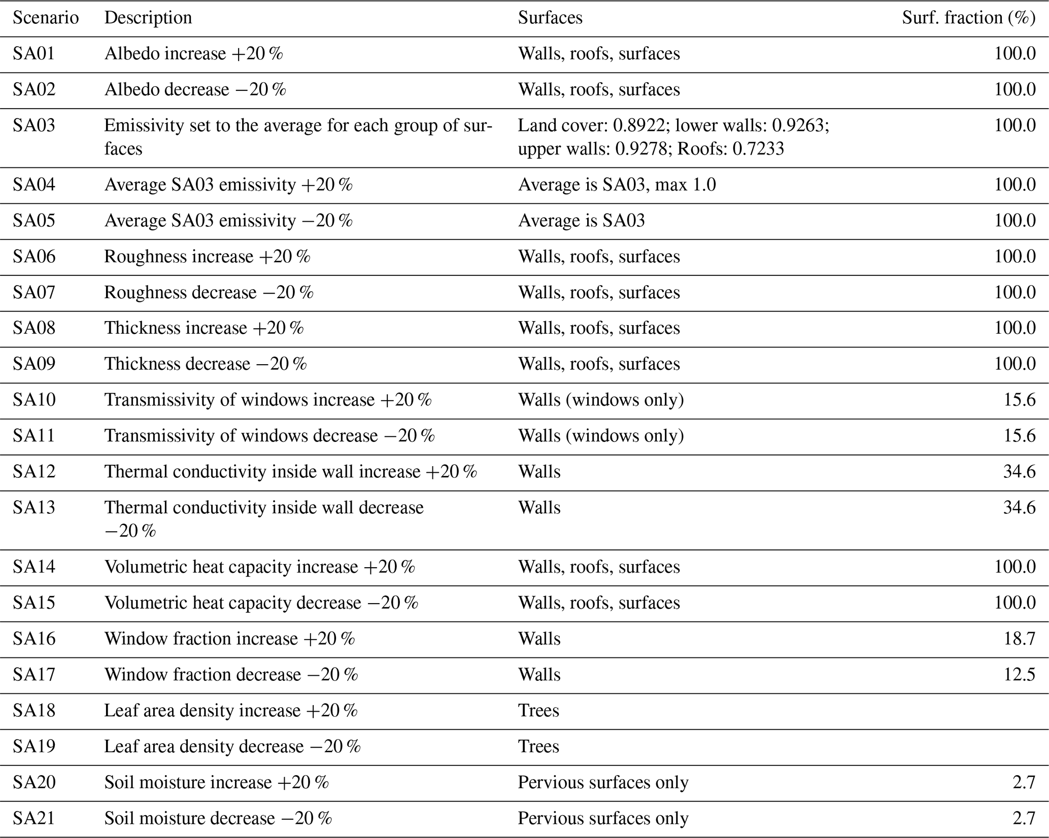
Since the analysis by Resler et al. (2017), the PALM modelling system has been extended with new features. According to the new functionalities, window and wall fractions were mapped for each building in BSM and more detailed plant canopy parameters were included in PCM. In total 21 scenarios (hereafter SA scenarios) were prepared that each change one specific parameter of the surfaces (and/or plant canopy) from the baseline simulation. Table 1 summarizes the parameter changes for the SA scenarios, the surfaces affected by the change and the fraction of the total surface area affected in the respective scenario.
Table 1Scenarios testing model sensitivity to changes in material parameters with fraction of affected domain surface area (column Surf. fraction). A detailed description of surfaces is in Sect. 2.3.
2.7.2 Urbanistic scenarios – sensitivity to urban heat island mitigation measures
The second group of scenarios was designed more from the urban planners' point of view, i.e. assessing the influence of (in)appropriate urban planning actions on improving thermal comfort and air quality. These scenarios present several measures typically taken into account when dealing with the UHI effect, such as greening or changes in the surface materials, simplified to distinguish individual influence (e.g. when changing roads to grass, the emissions are not changed). Although not necessarily realistic, these scenarios provide the urban planners with an assessment of the maximum potential influence of certain common types of urban development (e.g. removal of all trees versus planting trees everywhere). The design of the scenarios stemmed from discussion with various authorities of the City of Prague in the framework of the Urbi Pragensi project (http://www.urbipragensi.cz, last access: 13 July 2021). A detailed description of this group of scenarios (hereafter denoted by SB) is included in Table 2.
Table 2Scenarios testing sensitivity of the model results to UHI mitigation measures.
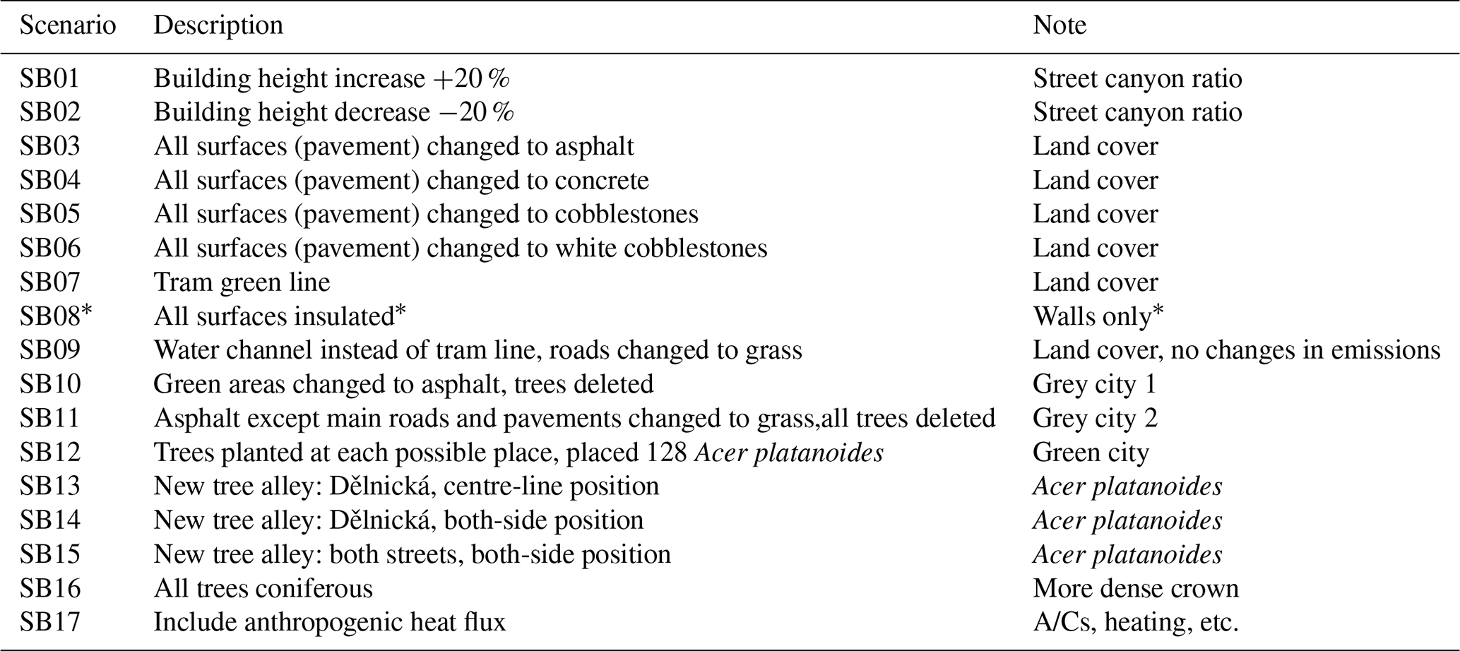
* Scenario SB08 was removed from further analysis because results were significantly affected by numerical instability solved in PALM revision 4240.
Due to the different nature of the two sets of scenarios, the analysis of the model results will be performed separately for the synthetic SA scenarios and urbanistic SB scenarios. However, some aspects of the analysis are common to both. The chaotic nature of the turbulent flow in the domain requires an application of time averaging which needs to be sufficiently long to smooth out turbulent fluctuations yet short enough to capture the diurnal variability. In the time series plots, we opted to show 10 min averaged values together with hourly moving averages. Summary tables (Table S02 in the Supplement), on the other hand, show 3 h averages along with daily averages, minima and maxima. One important aspect of the modelling setup which must be kept in mind when analysing the results is that the model spin-up period uses a constant dynamic and simplified energy model (see Sect. 2.2.1), and thus the initial thermal conditions (ground, wall and roof temperatures) are not in total agreement with temperatures that would have been obtained by a full model run. This can impose differences on the simulation behaviour in the first hours from standard behaviour in the following hours when this initial effect vanishes, which may limit the applicability of the results in the first few hours of the simulation after the spin-up. However, as most of the differences between respective simulations begin to appear after sunrise, this influence can be neglected.
Spatial variability is analysed by averaging over the whole domain as well as separately over several selected domain parts. A particular focus is on the two crossing streets and courtyards. For maps with point positions and area selections, see the Supplement (Figs. S01–S09). The most important variables for the end users were chosen as primary indicators. They include surface temperature, air temperature, PM2.5 concentrations and two biophysical temperature characteristics – mean radiant temperature (MRT) and physiological equivalent temperature (PET) – all at the height of the human body represented by the first 2 m high layer (for definitions and information about the implementation of MRT and PET in PALM, see Frölich and Matzarakis, 2020, and Krč et al., 2021).
All scenario simulations are analysed with respect to the baseline simulation (a model run with the original parameter values). Figure 2 shows the spatial distribution of basic variables in the domain for the baseline simulation.
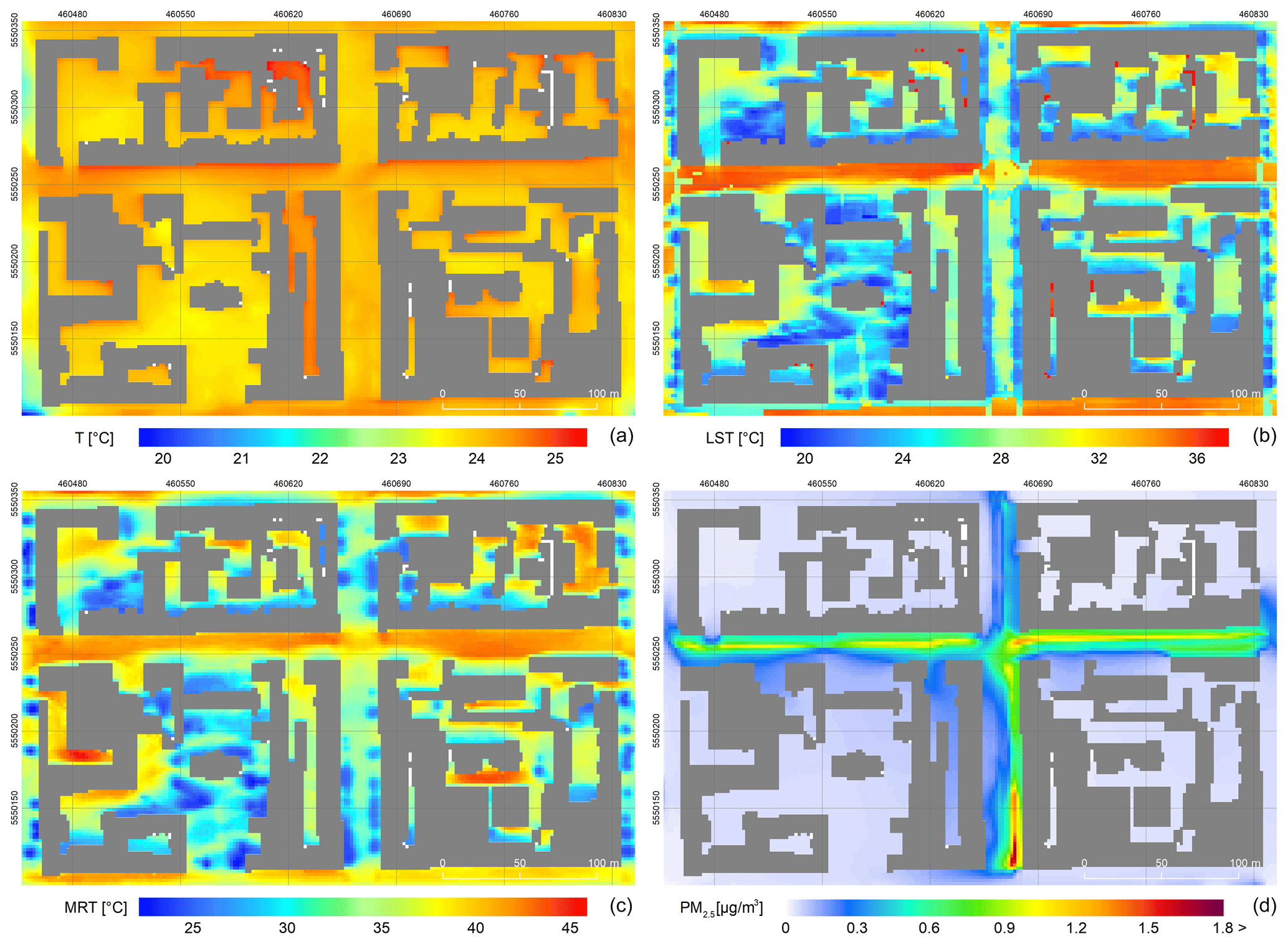
Figure 2Daily average spatial variability in (a) air temperature, (b) surface temperature, (c) mean radiant temperature – MRT – and (d) PM2.5 concentrations for the baseline simulation. Projection: WGS 84 / UTM zone 33N; layer with roofs is own data source.
3.1 Sensitivity to material parameters
In the first part of the assessment, we analyse the model sensitivity to the setting of building and material parameters such as albedo or roughness (SA scenarios). Figure 3 shows the sensitivity as differences between respective scenarios and the baseline simulation for air temperature (other variables are included in the Supplement as Figs. S11–S14) in 24 h averages. Table S02 in the Supplement summarizes all five analysed variables showing absolute values and differences (plus the relative difference) of each SA scenario from the baseline. Results are averaged for several areas: domain, east–west street (Dělnická), south–north street (Komunardů), both streets (Streets) and courtyards. In general, the following four parameters show the highest sensitivity for temperature: albedo (SA01, SA02), emissivity (SA03–05), thermal conductivity of walls (SA12, SA13) and volumetric heat capacity (SA14, SA15) with a median response of up to ±0.1 K (Fig. 3) and a maximum response reaching up to ±0.18 K in 3 h averages and up to ±0.4 K in 10 min averages for some parameters during the day (Table S02). Overall, the albedo setting (SA01, SA02) shows the highest sensitivity of all parameters in this group. The lowest sensitivity is observed for wall thickness (SA08, SA09), transmissivity of windows (SA10, SA11) and soil moisture (SA20, SA21). However, the reason for the low sensitivity to the changes in the soil moisture lies mainly in a low percentage of the green areas in the domain.
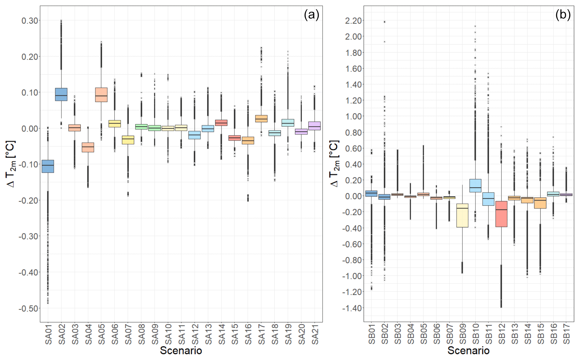
Figure 3Sensitivity of air temperature in SA (a) and SB (b) scenarios. Values represent grid box differences (scenario − baseline) of 24 h averages in the first 2 m high layer. Box colours indicate related scenarios (e.g. blue for changing albedo, orange for changing emissivity). Whiskers: values within 1.5× the interquartile range; crosses: outliers.
The daily cycle of air temperature also has an imprint on the relative importance of respective parameters throughout the day. Parameters used in incoming radiation routines (namely albedo; SA01, SA02) are the most sensitive ones in the middle of the day, when the radiative balance is governed mostly by incoming short-wave radiation. During the night, emissivity (SA03–05) and the heat capacity of walls (SA14, SA15) play a major role (see Table S02); thus sensitivity to these parameters is higher then. Some parameters show quite high sensitivity only for short periods during the day. For example the window fraction shows low sensitivity in the morning hours, after which it increases at around 09:00–12:00 UTC (11:00–14:00 local time) and peaks in the early evening at around 18:00–21:00 UTC (see SA16–17 in Table S02). In this particular case, given that the response to a lower window fraction is an increase in temperatures and vice versa, the most likely explanation is the difference in heat storage between windows (very low) and walls (higher), which has a prevalent influence in low-sun periods of the day.
Air temperature, though fundamental for physical evaluation, is not necessarily the best quantity for evaluating biophysical properties, namely thermal comfort. For this purpose, MRT and PET variables combining other relevant physical variables (radiation, humidity, airflow, etc.) are used. Given the combination of various influences, MRT and PET often show sensitivity higher than but inverse to that of the air temperature. As a demonstration we show this for the two most prominent scenarios, SA01 and SA02. In SA01, the albedo is increased by 20 %, which results in a decrease in daily surface temperatures by 0.5 K and a decrease of around 0.1 K for air temperature. On the other hand, by increasing reflection at the surfaces, this change increases both MRT and PET by 0.6 and 0.3 K, respectively. In daily maxima, the increase in both biometeorological variables is even more prominent and reaches up to 1.7 and 1.6 K, respectively. Decreasing albedo by 20 % in SA02 has a similar effect in terms of absolute numbers but with the opposite sign.
Influence on air quality, represented here by changes in PM2.5 concentrations at the first model layer, originating from emissions from local transportation, is generally much less pronounced in all scenarios. For the dominant parameters, such as albedo or emissivity, we still observe a similar general tendency to increase (decrease) PM2.5 values with increased (decreased) albedo (emissivity). This is opposite behaviour to that of the surface and air temperatures, and it is likely primarily caused by connected changes in the flow regime as illustrated in Figs. 4 and 5 by a decrease (increase) in wind speed with increased (decreased) albedo (also discussed in e.g. Žák et al., 2016). It should be noted here that, due to non-linearity, the response to the symmetrically constructed scenarios (e.g. SA01 and SA02) need not be symmetric in the spatial distribution as also illustrated in Figs. 4 and 5. For example, the changes in wind speed are more pronounced in the western part of the west–east-oriented street and at the crossroads when decreasing the albedo. Furthermore, the sensitivity in some places, e.g. the northern part of the north–south-oriented street or some courtyards, is such that decreasing or increasing albedo both result in increasing wind speed.
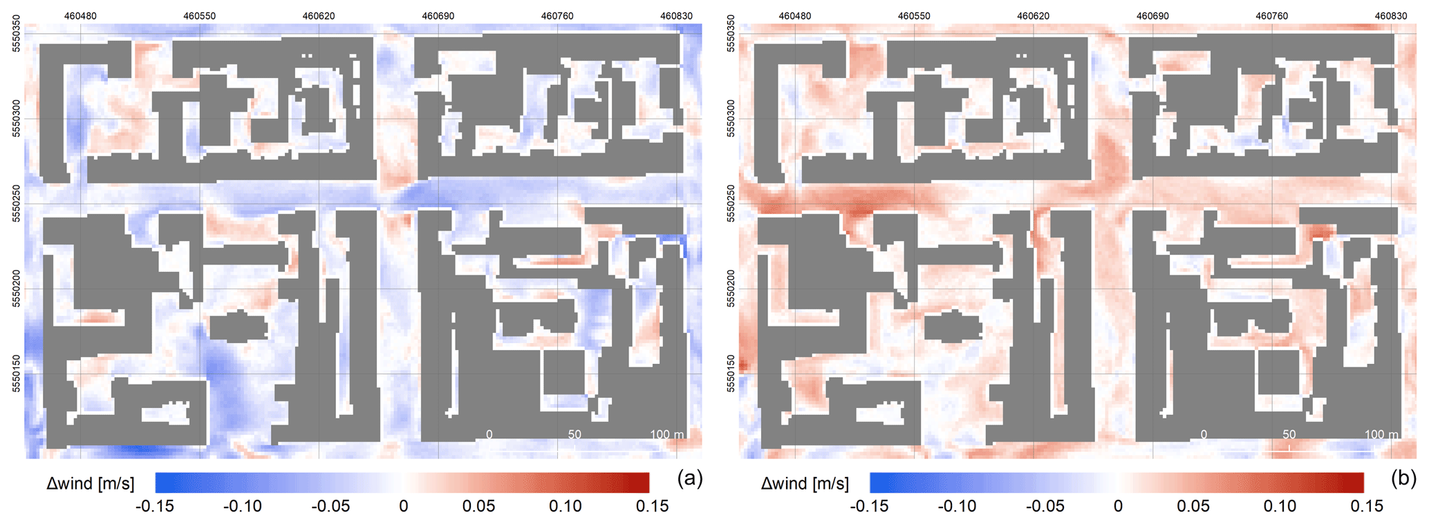
Figure 4Daily average sensitivity of horizontal wind speed (1 m) expressed as the difference between scenario and baseline. (a) Scenario SA01 (albedo increased by 20 %); (b) scenario SA02 (albedo decreased by 20 %). Projection: WGS 84 / UTM zone 33N; layer with roofs is own data source.

Figure 5Daily average profiles of w2 (plotted as the difference: scenario − base case) averaged over the two main streets: the north–south-oriented Komunardů (a) and the west–east-oriented Dělnická (b).
Long-term average changes in PM2.5 concentrations are generally small and with the exception of singular peaks (Fig. 6) lie within ±5 % in most of the domain. The temporal evolution of the response, however, may also differ depending on the geometric configuration as is also evident from Fig. 6 which shows spatially averaged values for the two main streets in the albedo-changing SA01 and SA02 scenarios. The difference between the two scenarios is more pronounced in the north–south-oriented Komunardů street in the afternoon hours, while in the morning hours, the difference is larger in the west–east-oriented Dělnická street.
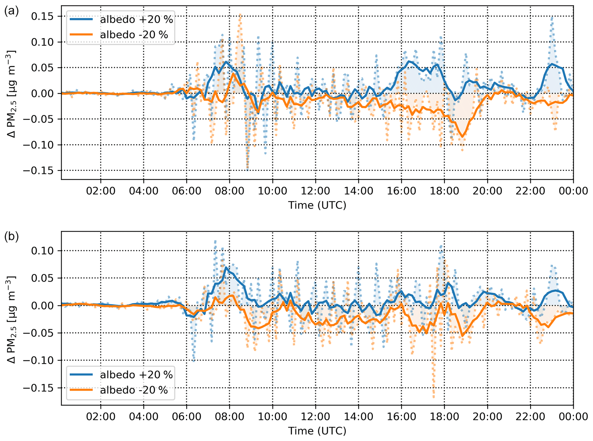
Figure 6Changes in PM2.5 for the north–south-oriented Komunardů street (a) and the west–east-oriented Dělnická street (b) in scenarios SA01 (albedo +20 %, blue) and SA02 (albedo −20 %, orange). Dotted lines: 10 min values; solid lines: 1 h moving average.
The parameters we analyse influence the results mainly by changing the energy balance of the horizontal and vertical surfaces in the model domain. Air temperature changes are then mainly driven by the transfer of heat between these surfaces and air. In this context, we will now focus on the effect on surface temperatures. The highest sensitivity of surface temperature is observed in the same scenarios as for air temperature: albedo SA01 and SA02 (Fig. 7), emissivity SA03–05, thermal conductivity SA12 and SA13, and volumetric heat capacity SA14 and SA15. The average response reaches up to ±0.5 K and the 3 h maxima reach up to ±0.9 K with albedo changes (SA01, SA02) and decreased emissivity (SA05).
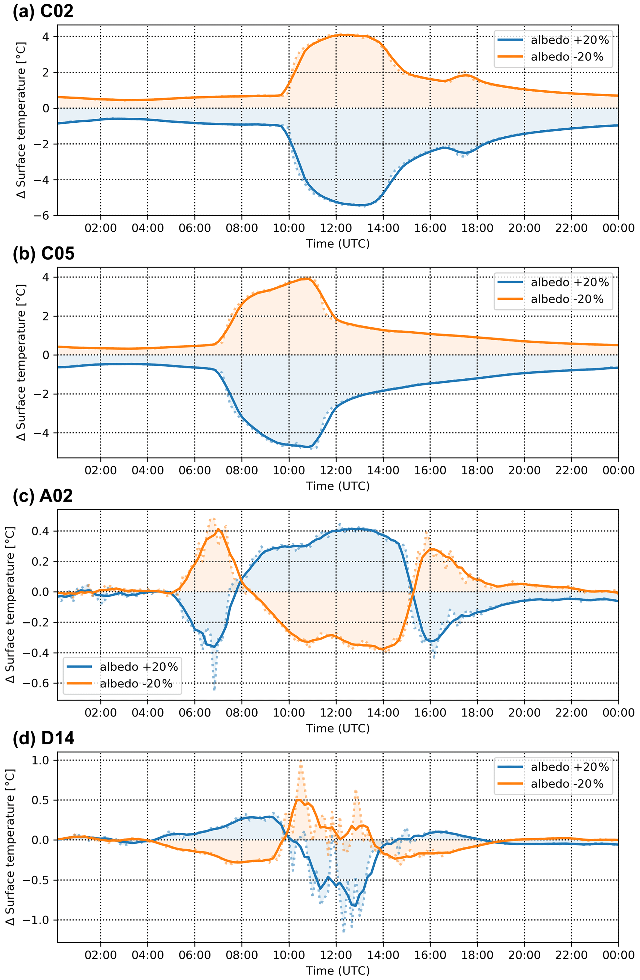
Figure 7Differences in surface temperature in evaluation points C02 (a), C05 (b), A02 (c) and D14 (d) for albedo-changing scenarios SA01 (blue) and SA02 (orange). Dotted lines: 10 min values; solid lines: 1 h moving average.
The model response to the surface parameters is also dependent on the location. This stems mainly from the differences in the radiation budget during the day caused by positioning of urban elements (buildings and trees). At individual points, the differences in surface temperature with respect to the base case reach up to ±4 K in shorter periods in the albedo change scenarios SA01 and SA02 (e.g. points C02 and C05 in the upper two panels of Fig. 7).
Air temperature showed a rather small sensitivity to changes in soil moisture, which we attribute to a rather low percentage of green areas in the domain. However, small areas covered with or in the direct vicinity of vegetation are influenced significantly as shown in Fig. 8 for point F03. For this and other similar points (e.g. F02, F04, H02), changes in soil moisture show much higher sensitivity in surface temperature and biometeorological indicators (in the additional outputs; see “Code and data availability” section for URL) around noon with differences reaching up to 6 K. For other examples of the influence of soil moisture on surface temperature in a validation study of a real city environment, see also Resler et al. (2020).
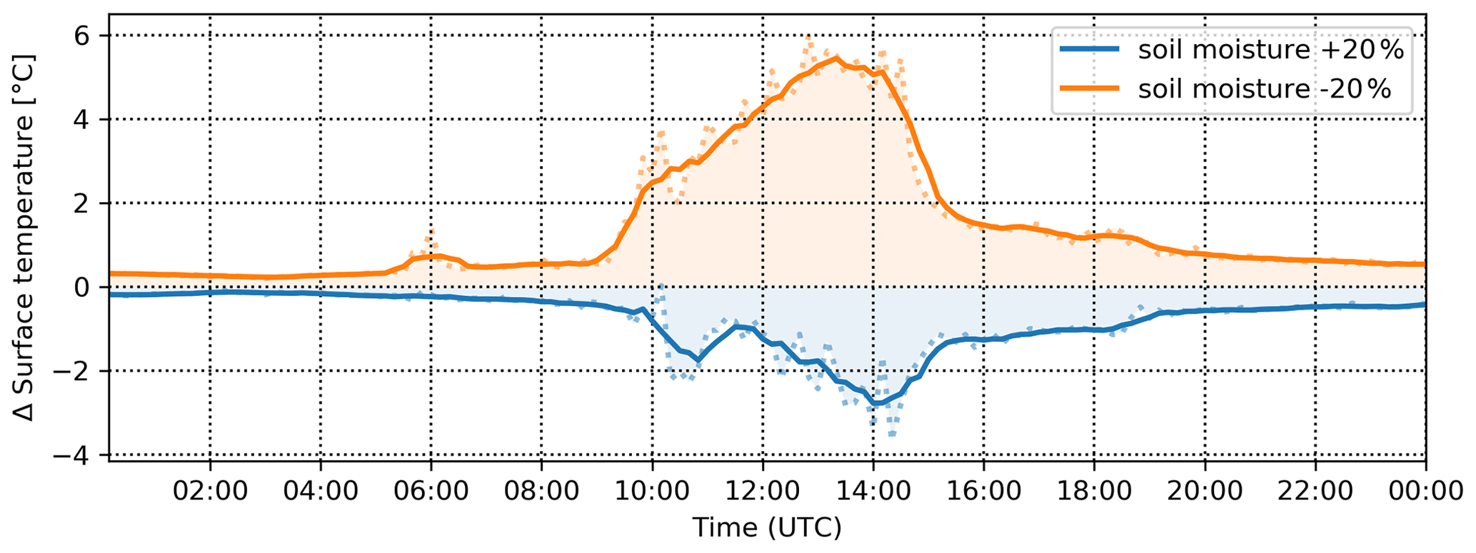
Figure 8Soil moisture sensitivity of surface temperature difference for scenario SA20 (blue line) and SA21 (orange line) at point F03. Dotted lines: 10 min values; solid lines: 1 h moving average.
In some parts of the domain, the typical daily cycle of the differences is even reversed in certain periods of the day. A typical example of this behaviour is the sensitivity of surface temperature to albedo changes (Fig. 7). While most surfaces show an expected increase (decrease) in temperature with the decrease (increase) in albedo (typical examples are points C02 and C05 in Fig. 7), some analysis points (e.g. A02, A04, B04, B06, D13, D14) show a reverse influence. Two examples of the inverse behaviour are illustrated in Fig. 7 for points A02 and D14 (lower two panels), clearly showing higher (lower) albedo resulting in higher (lower) surface temperatures during some parts of the day, when presumably increased (decreased) reflection from other surfaces brings more (less) SW radiation at these points compared to for the base case. The difference in the incoming SW radiation for points A01 and A02 is demonstrated in Fig. S15 comparing the S01 (blue) and S02 (orange) scenarios with the baseline (black): the A01 point (solid lines) receives less incoming radiation with increased albedo, while for the A02 point (dashed line) the incoming radiation is increased with increased albedo due to reflection from opposite surfaces in the corresponding time.
High spatial variability is also evident from other scenarios and shows the importance of using very high resolution models for local studies. As can be seen from, for example, figures for the emissivity changing scenarios SA03–SA05 (in the additional outputs; see “Code and data availability” section for URL), while the spatially averaged response shows mostly a simple daily cycle with a maximum change around noon, some individual points (e.g. A02, A04) show maxima in the morning and afternoon hours, while around noon the effect diminishes. Depending on the individual surface radiation budget given by the incoming solar radiation and reflections from other surfaces, some points experience a delayed peak in the afternoon hours with an inverse response; i.e. increased emissivity leads to an increase in temperatures (C04, D02).
3.2 Sensitivity to urban heat island mitigation measures
The second part of the sensitivity analysis focuses on the urbanistic scenarios. These scenarios include UHI mitigation measures, which planners and decision makers might apply to improve the bioclimatic situation in the city during high-temperature conditions, especially heatwaves. Typically considered measures include planting trees or changing surface materials (Table S02). As a contrast to SA scenarios, SB scenarios usually require changing more than one parameter at once. For instance, replacing concrete with grass results in changes in albedo, emissivity and roughness as well as in other parameters.
Sensitivity of the model response to SB scenarios is also summarized in Table S02. The most significant changes in surface temperature are observed in scenarios SB09 (land cover changes), SB10 (grey city 1) and SB11 (grey city 2), while for air temperature (Fig. 3), SB09–11, SB12 (green city with many planted trees), SB14 (new tree alley with both-side position on the Dělnická street) and SB15 (new tree alley with both-side position on both streets) show the strongest sensitivity. Scenario SB09, in which grass replaces roads and a tram line is replaced with a water channel, shows a decrease in surface temperatures by up to 3.0 K and in air temperature by up to 0.3 K. Grey-city scenarios SB10 and SB11 (Fig. 9), on the other hand, tend to increase temperatures significantly with 3 h maximum differences exceeding 2 K on the horizontal surfaces, whereas for air temperatures an increase by 0.3 and 0.1 K, respectively, is found. However, this difference between the two scenarios is dependent on the area of interest. For example, in the north–south street (Komunardů), the change in air temperatures is much more consistent between the scenarios, with maxima reaching +0.5 K in the late afternoon (Table S02 in the Supplement).
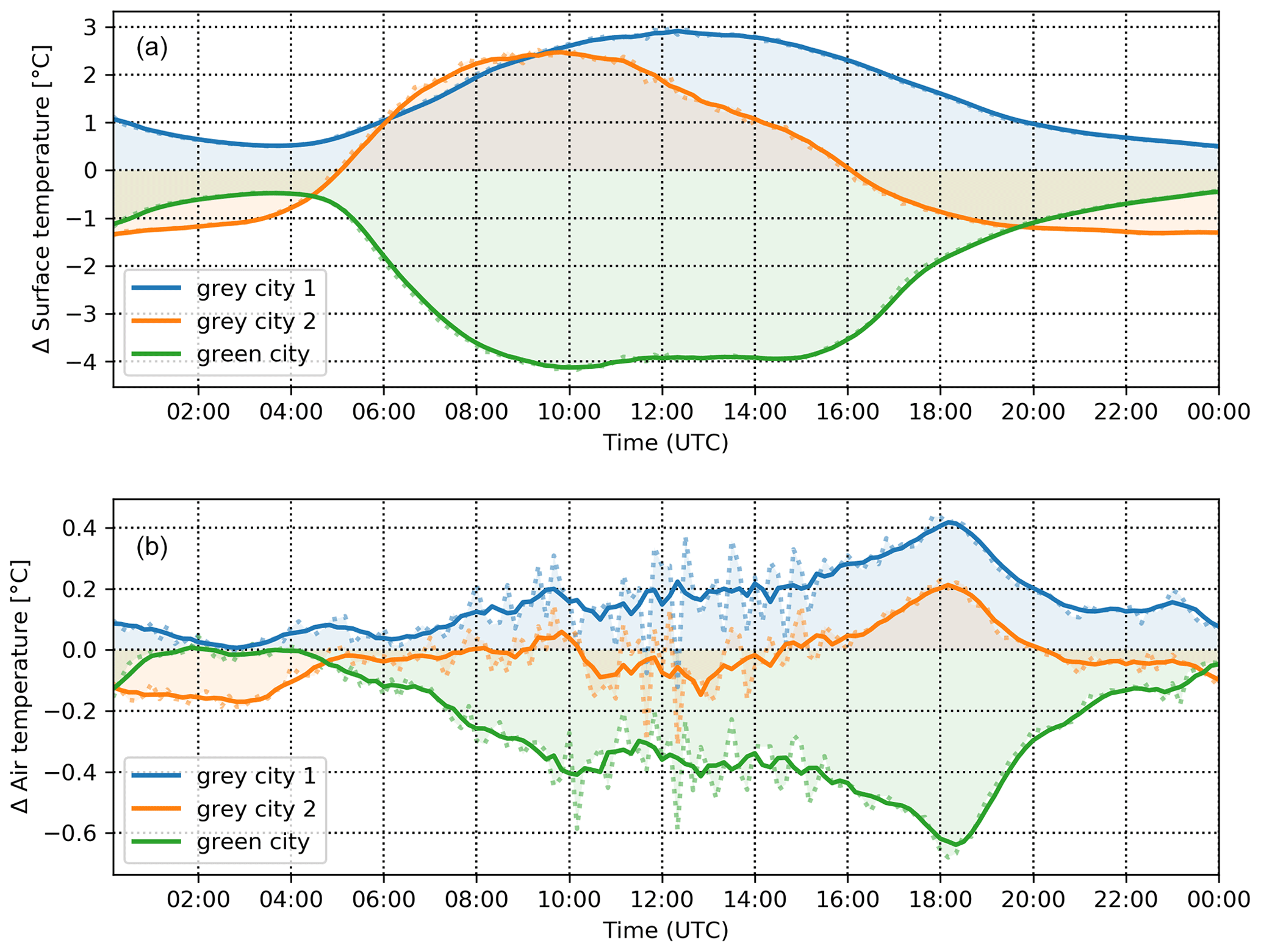
Figure 9Domain-averaged differences in the surface temperature (a) and air temperature (b) for grey-city scenarios SB10 (blue) and SB11 (orange) and green-city scenario SB12 (green). Dotted lines: 10 min values; solid lines: 1 h moving average.
Scenario SB12 (green city with many planted trees) appears the most effective in decreasing temperature during the day with surface temperature cooler by up to 4.0 K and air temperature cooler by almost 0.5 K (Fig. 9). The effect is smaller during the nighttime, when the decrease in temperature is 0.8 and 0.12 K, respectively. Instead, scenario SB09 and even SB11 (removing trees but increasing grass-covered area) show decreases of more than 1.0 and 0.15 K in the surface and air temperatures.
In terms of thermal comfort, the two analysed characteristics (MRT and PET) show behaviour qualitatively similar to the physical temperatures. Again, the SB12 scenario (green city with many planted trees) shows the most effective reduction with a maximum decrease of around 9 K in MRT and 4 K in PET in the entire domain. However, the effect varies considerably in space. The strongest change is observed in the west–east-oriented Dělnická street, while the north–south-oriented Komunardů street shows a much smaller decrease of 0.0–1.2 K (Fig. 10). This difference can be partly attributed to the geometric orientation of the streets and consequent differences in insolation during the day but also to the actual number of trees added with respect to the base case, in which more trees already grow in the Komunardů street. Similar behaviour is shown in the SB13–SB15 scenarios (new-tree-alley scenarios) with decreases of up to 4.0 K in MRT and 1.6 K in PET on average.
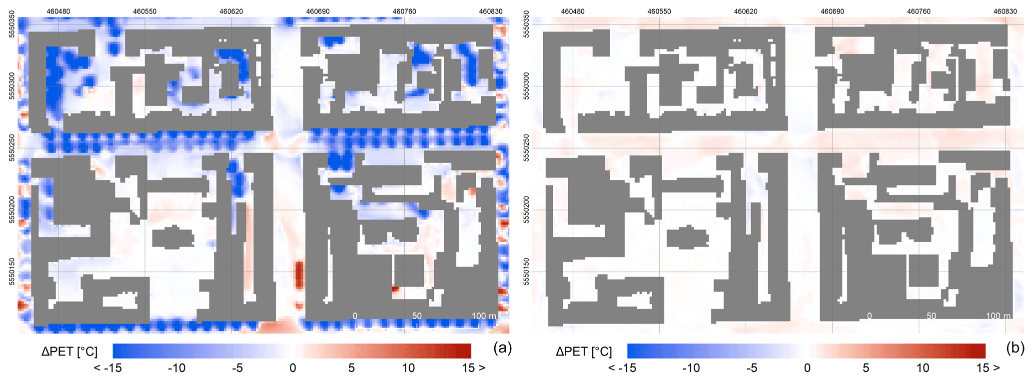
Figure 10Example of spatio-temporal variability of 3 h PET differences for green-city scenario SB12 at 09:00–12:00 UTC (a) and 21:00–24:00 UTC (b). Projection: WGS 84 / UTM zone 33N; layer with roofs is own data source.
On the other hand, SB10 and SB11 scenarios (grey city 1 and 2) show a significant increase in both biophysical properties. The MRT is increased by 8 K (5 K) and PET is increased by 3 K (1.6 K; see Fig. 11) at around noon in the entire domain in SB10 (SB11). Similarly to the previous comparison, there is a marked spatial difference throughout the domain. However, the effect is strongest in the Komunardů street, with an increase of over 12 (MRT) and 3 K (PET), and courtyards (over 9 K and 4 K), while in the Dělnická street, the increase is only around 3 K in MRT and 1 K in PET.
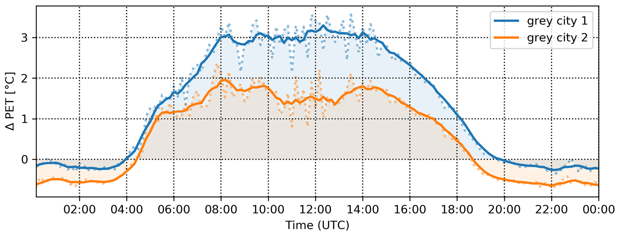
Figure 11Domain-averaged differences in PET for grey-city scenarios SB10 (blue) and SB11 (orange). Dotted lines: 10 min values; solid lines: 1 h moving average.
Unlike for the SA sensitivity cases, PM2.5 shows a significant dependence on the measures applied. However, the influence is almost universally inverse to the one for temperature. Generally, decreasing surface/air temperature increases PM2.5 concentrations by suppressing ventilation and turbulent mixing. On average the strongest effect is observed in the SB12 (green city with many planted trees) and SB15 (planting the highest number of trees) scenarios (Fig. 12), which show an increase of 24 % and 21 % in PM2.5 with maxima over 30 % in the late afternoon hours. Scenarios that simulate planting trees only in the Dělnická street, SB13, one tree alley in the centre) and SB14 (tree alleys on both sides of the street), show similar responses in terms of the shape of the daily cycle but with a lower overall increase (Fig. 12); on average, these scenarios show an increase of 5 %–14 % in PM2.5 concentrations, with maxima reaching almost 20 % for SB14 and 10 % for SB13 scenario (Fig. 12).
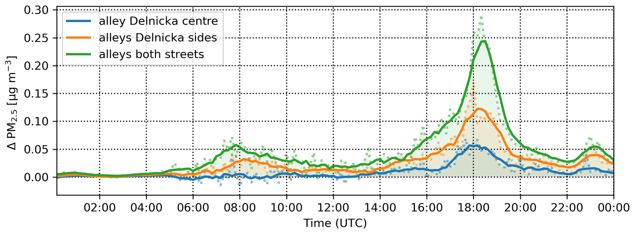
Figure 12Domain-averaged differences in PM2.5 for new-tree-alley scenarios SB13 (blue), SB14 (orange) and SB15 (green). Dotted lines: 10 min values; solid lines: 1 h moving average.
Interestingly, over the perpendicular Komunardů street with no new trees planted, the concentrations tend to decrease throughout most of the day, although this decrease is mostly concentrated at the crossroads; for the street sections north and south further away from the crossroads, no significant changes are modelled. The effect is connected to spatial changes and intensification of the street canyon eddy induced by the tree-obstructed Dělnická street which acts effectively as a part of the street canyon (not shown). The grey-city scenarios SB10 and SB11 conversely show decreased PM2.5 concentrations of around 20 % in the afternoon and evening. Considering the spatial differences, the highest decrease is observed in the Komunardů street (over 50 %; see Fig. 13).
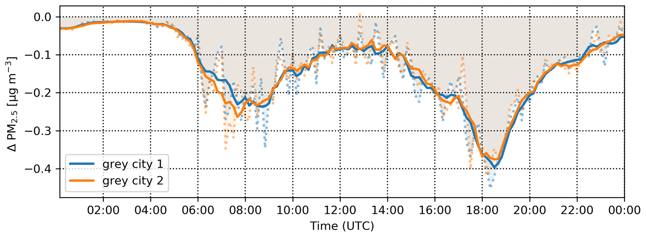
Figure 13Differences in PM2.5 in the Komunardů street for a grey-city scenarios SB10 (blue) and SB11 (orange). Dotted lines: 10 min values; solid lines: 1 h moving average.
4.1 Discussion
In this work, we assessed the sensitivity of air and surface temperature, MRT, PET, and PM2.5 within the PALM model system 6.0 as a response to the modification of basic surface material parameters as well as to common UHI mitigation strategies. For this we performed a set of semi-idealized model simulations for a diurnal cycle in a city quarter in Prague.
The first set of scenarios, designed to examine the sensitivity to the parameter settings, shows the importance of the correct setting of the radiation parameters of albedo and emissivity. This can be expected as the solar radiation is the main source of energy in the surface energy budget. Additionally, unlike some other parameters, radiation parameters are changed for all surfaces.
In addition to albedo and emissivity, thermal conductivity of walls and volumetric heat capacity of the materials play an important role. Other parameters show a limited average effect on the diurnal timescale, which, however, can be quite significant during some parts of the day, such as surface roughness in the morning hours and the window fraction in the evening. Changing soil moisture by 20 % is shown to be negligible overall in the context of the chosen domain, with only a small percentage of the surface covered by vegetation (see Table 1), except for surface temperature during the high-sun part of the day. Individual parts of the domain with larger coverage of vegetation show greater influence. Note that we investigated only the short-term response of the urban canopy on the outlined modifications. The trends might be more prominent if long-term storage of energy in the materials were considered, i.e. when simulating a full heatwave.
The second part of the sensitivity analysis focused on the UHI mitigation measures. One of the commonly considered measures is to paint surfaces white to increase surface albedo. However, our results indicate that this is only effective for lowering the surface and air temperature. In contrast, the biophysical indicators MRT and PET tend to be negatively affected; i.e. thermal comfort in the street deteriorates due to increasing the amount of reflected radiation (note that the effect can be different on purely horizontal surfaces such as roofs). Improving both physical and biophysical temperature indicators requires the application of other measures, such as urban greening at the same time. Similar findings have also been reported in, for example, a meta-analysis of 52 ENVI-met simulations by Tsoka et al. (2018) and Yang et al. (2015), who stress the need for precaution when adopting high-reflectivity surfaces, or Aflaki et al. (2017), who found low-albedo vegetation effective in reducing mean radiant temperature.
Urban vegetation is found to be the most effective measure when considering reduction in both physical and biophysical temperature indicators. Conversely, grey-city scenarios that reduce the amount of urban vegetation show significant worsening of the thermal comfort. Urban greenery is very often found to be an effective mitigation tool for the UHI phenomenon; for example a recent study by McRae et al. (2020) reports vegetation-induced cooling of more than 3 ∘C in an ENVI-met simulation. However, some studies (e.g. Wang et al., 2016; Tsoka et al., 2018; or Makido et al., 2019) show that for the best effect it is necessary to combine several measures and also to consider that different parts of the city may need different measures.
One of the most important results of our analysis is that it confirms opposite behaviour of thermal comfort and air quality indicators (see example in Fig. 14). Observed in both types of scenarios, the PM2.5 concentrations typically increase with decreasing temperatures and vice versa. The main reason for this behaviour is decreased ventilation in the street canyon due to airflow blocking. The decreased vertical turbulent transport due to reduced urban canopy temperatures and thus buoyancy can play a role too, as shown by Huszár et al. (2018b, 2020), who found significant PM decreases due to urban-canopy-induced vertical eddy diffusion. However, in these simulations, only aerosol passive transfer was taken into account, and thus the results may be different for other air quality indicators, e.g. when considering the influence of changing reaction coefficients and a decrease in solar radiation for ozone chemistry (Huszár et al., 2018a).
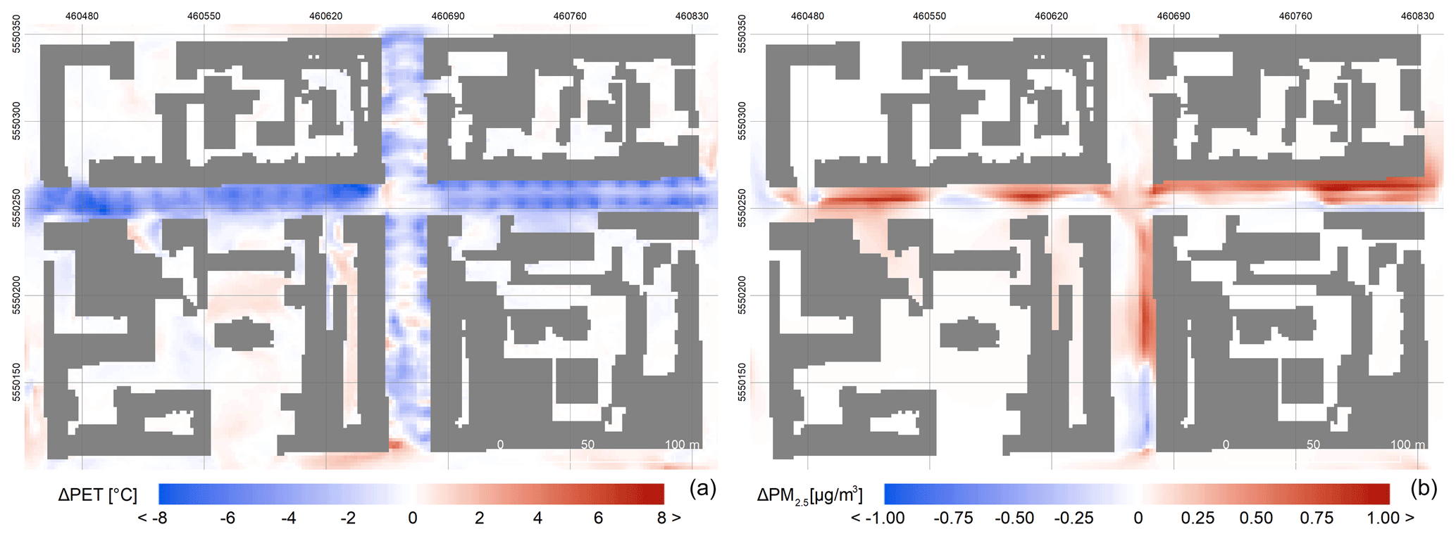
Figure 14Example of opposite behaviour of thermal comfort and air quality indicators represented by average daily difference in PET and PM2.5 for new-alley scenario SB15.
The PM2.5 concentrations in Fig. 14 also show the important added value of the high-resolution CFD models for urban modelling compared to parameterized urban schemes in NWP and climate models or radiation models. In this case it is the spatial variability within the streets. As can be seen, the combined radiative and dynamical effects manifest in quite a heterogeneous response where (in this particular case) the increase in concentrations is most prominent in the northern half of the Dělnická street, while in some parts on the southern side the model shows a decrease in concentrations. In the Komunardů street, the response shows very small changes in the upper section of the street while in the lower section the model shows almost a see-saw response with increased concentrations in the upper half and a decrease in the lower half of the section.
4.2 Study limitations
This study applied the PALM model revision 4093. The model itself and the configuration applied for this study have some limitations, with the following being the most important ones in our case:
-
The model is configured without the PALM-4U building energy model (BEM), and the building inner temperature is considered constant (300 K) during the simulation. The impacts of the absence of a more complex indoor model differ in the summer and winter seasons. In winter, assuming that the rooms are heated to the exact prescribed temperature by either direct local heat sources or long-distance heating with the heating plant being outside the modelled domain, the model adds correct heat fluxes to the insides of the buildings, albeit not providing the amount of heating energy consumed among its outputs. In summer, the constant indoor temperature can be seen as a simplification for buildings without air conditioning where the wall insulation and wall heat capacity dampen most of the daily temperature difference, as long as the inner temperature is realistic and the daily total net heat flux is near zero. Buildings with air conditioning need a more complex indoor model with correctly placed heat exchangers (windows for individual A/C units and roofs for central A/C systems). For the simulated domain, there was no information available about the number and placement of A/C systems, with the majority of the buildings being old apartment houses with presumably no central A/C systems and no visible individual A/C units at windows. For long-term simulations, missing waste heat which could be provided by PALM's indoor model will be important although, given the short timescale of the present study simulations, the indoor model should not affect the outcome. The outer wall layers react very fast to changes in the surface energy balance, but the inner wall layers have large inertia, so nothing is likely to change if the indoor temperature changes in time.
-
The model sensitivities are tested only during meteorological conditions of heatwave episodes as the main focus is on simulation of the UHI mitigation measures. Only the short-term response of the urban canopy was investigated. The behaviour, including the long-term response, during other seasons and weather conditions can and probably will differ from presented results.
-
The simulations do not consider any chemical reactions or aerosol dynamic processes of air pollutants; only the dispersion of traffic-related PM2.5 is considered. Moreover, the boundary conditions of the chemical species on the parent domain were set to zero. This experiment design was selected as the focus of the study is on the sensitivity of the concentrations to the local conditions. The time needed for secondary organic aerosol (SOA) formation is much longer than the typical time the chemical species spent in the studied domain (e.g. Du et al., 2018, or Tang et al., 2018). The consequence is that the SOA concentration field is almost constant over the studied domain. It means that even though the SOAs constitute an important part of the PM2.5, their omission does not change the differences in PM2.5 between particular scenarios.
-
This version initiates the building wall properties through the
building_2dproperty in the model static driver; i.e. the wall properties are set to the roof grid cell over the wall (i.e. border grid cells of the roof). This leads to the following two simplifications.-
The properties of the wall can be set only in two height zones, and the corner grid cells set the properties of two surface grid cells corresponding to different walls.
-
The roof properties in the border grid cells are initialized to the wall properties. This limitation leads to artefacts in roof and wall surface temperature and heat fluxes. This drawback was removed in later versions (model revision 4240 and later) by implementation of reading separate properties for individual surface cells from the new static driver variable building_surface_pars.
-
-
The ventilation of very tight areas surrounded by high buildings is underestimated by the model, and the temperatures and concentrations of pollutants become unrealistically high in some circumstances. It is known that higher concentrations can be expected in enclosed spaces due to low turbulence (Gronemeier and Sühring, 2019). This problem was addressed in the model revision 4110. For the purpose of this analysis, these small areas were excluded from the evaluation.
Taking these limitations into account, we consider the simulation to produce plausible results both in actual values and in their spatial and temporal distribution in the baseline simulation. This was confirmed by comparing the general agreement of the results to the previously validated simulations (Resler et al., 2017) in the preparatory stage of this experiment (not shown). Obviously, extensive validation of the model against observations is beyond the scope of this paper. For systematic validation of the current model version, we refer the readers to the accompanying paper by Resler et al. (2020).
The LES is quite demanding in terms of computational power, especially when compared with its RANS-based counterpart. Since we did not perform evaluation of the model results against observations in this study, it cannot be shown whether the additional computer resources used bring about an improvement in the model performance. However, numerous studies have been published showing the added value of LES for street canyon simulations especially where air quality is concerned. For example Gousseau et al. (2011), Salim et al. (2011), and Tominaga and Stathopoulos (2011) evaluated LES and RANS simulations against wind-tunnel measurements in street canyon experiments, and all conclude that LES shows better performance. More recently, Antoniou et al. (2017) studied outdoor ventilation in a real urban area of Nicosia, Cyprus, again evaluating RANS simulations and LES against wind-tunnel measurements. They conclude that LES shows smaller deviations from the measurements than RANS simulations for mean wind speed and turbulence intensity.
4.3 Conclusions
In conclusion, this analysis shows that the proper setting of urban surface parameters is crucial for high-resolution LES models of the urban environment and that collecting this large number of data is an essential part of the modelling technique. High temporal and spatial variability also shows the importance of using truly local information for each area of interest. This fact also poses certain limits on the applicability of the findings of this study for other locations. On the one hand, the above comparisons with other studies showed qualitatively similar results in average behaviour, and in this sense we can expect similar average results in other densely built urban areas in similar climatic conditions (e.g. many European cities). However, quantitative assessment is largely dependent on the location studied, namely the physical configuration of buildings and other urban components, and thus the actual sensitivity values may differ between locations. This is evident, for example, from the albedo scenarios, for which the response in some locations was reversed depending on the geometrical configuration or soil moisture scenarios, when the small amount of existing vegetation limits the potential response of the system to changing soil moisture in larger areas. When assessing the very local influences, e.g. pedestrian-level thermal comfort, the local settings play a major role and thus need to be considered for proper evaluation.
Altogether, the LES method proves to be an asset thanks to its capability to fully resolve the flow and to consider heterogeneity in the modelling domain. Hence, LES modelling results can be really applied to support urban planning when aiming to mitigate the UHI phenomenon in urban neighbourhoods.
The PALM model system is freely available from http://palm-model.org (last access: 30 March 2020) and distributed under the GNU General Public License v3 (http://www.gnu.org/copyleft/gpl.html, last access: 30 March 2020). The model source code of version 6.0 in revision r4093 used in this article is also available via https://doi.org/10.25835/0068421 (Geletic et al., 2020).
Model configuration files; input data needed for running the simulations; and model output postprocessing code, i.e. extraction and visualization scripts, together with necessary data extracted from the raw model outputs and additional outputs, are available for download at http://hdl.handle.net/11104/0309669 (Library of Czech Academy of Sciences, 2020).
The supplement related to this article is available online at: https://doi.org/10.5194/gmd-14-4443-2021-supplement.
MB was the main coordinator of manuscript proceedings and responsible for the general topic of the paper and the analysis of results. All co-authors contributed to the manuscript text. KE configured and processed WRF simulations used for preparation of boundary conditions; JG was involved in geodata preprocessing, result postprocessing and data mining. JR and PK were strongly involved in the PALM model setup and processed the PALM simulations; JR also participated in the experiment design. VF, FKS, MS and BM participated in the general topic, discussion and text preparation. NB, MA and MK are specialists in air quality modelling and participated in this field of study.
The authors declare that they have no conflict of interest.
Publisher’s note: Copernicus Publications remains neutral with regard to jurisdictional claims in published maps and institutional affiliations.
The simulations were performed on the HPC infrastructure of the Institute of Computer Science (ICS) of the Czech Academy of Sciences supported by the long-term strategic development financing of the ICS (RVO 67985807) and partly in the supercomputing centre IT4I which was supported by the Ministry of Education, Youth and Sports through the Large Infrastructures for Research, Experimental Development and Innovations project IT4Innovations National Supercomputing Center – LM2015070.
Financial support was provided by the Operational Program Prague – Growth Pole of the Czech Republic project Urbanization of weather forecast, air-quality prediction and climate scenarios for Prague (CZ.07.1.02/0.0/0.0/16_040/0000383), which is co-financed by the EU. The co-authors Björn Maronga, Farah Kanani-Sühring and Matthias Sühring were supported by the German Federal Ministry of Education and Research (BMBF) under grant 01LP1601 within the framework of Research for Sustainable Development (FONA; https://www.fona.de/de/, last access: 27 May 2021). Financial support was also provided by the Norway Grants and Technology Agency of the Czech Republic project TO01000219: Turbulent-resolving urban modeling of air quality and thermal comfort.
This research has been supported by the European structural and investment funds (grant no. CZ.07.1.02/0.0/0.0/16_040/0000383), the German Federal Ministry of Education and Research (grant no. 01LP1601A), and the Norway Grants and Technology Agency of the Czech Republic (Turbulent-resolving urban modeling of air quality and thermal comfort (grant no. TO01000219)).
This paper was edited by Simon Unterstrasser and reviewed by two anonymous referees.
Aflaki, A., Mirnezhad, M., Ghaffarianhoseini, A., Ghaffarianhoseini, A., Omrany, H., Wang, Z., and Akbari, H.: Urban heat island mitigation strategies: A state-of-the-art review on Kuala Lumpur, Singapore and Hong Kong, Cities, 62, 131–145, https://doi.org/10.1016/j.cities.2016.09.003, 2017. a
Ai, Z. T. and Mak, C. M.: Modeling of coupled urban wind flow and indoor air flow on a high-density near-wall mesh: Sensitivity analyses and case study for single-sided ventilation. Environ. Modell. Softw., 60, 57–68, https://doi.org/10.1016/j.envsoft.2014.06.010, 2014. a
Antoniou, N., Montazeri, H., Wigo, H., Neophytou, M. K. A., Blocken, B., and Sandberg, M.: CFD and wind-tunnel analysis of outdoor ventilation in a real compact heterogeneous urban area: Evaluation using “air delay”, Build. and Environ., 126, 355–372, https://doi.org/10.1016/j.buildenv.2017.10.013, ISSN 0360-1323, 2017. a
Arnfield, A. J.: Two decades of urban climate research: a review of turbulence, exchanges of energy and water, and the urban heat island, Int. J. Climatol., 23, 1–26, https://doi.org/10.1002/joc.859, 2003. a
Ashie, Y. and Kono, T.: Urban‐scale CFD analysis in support of a climate‐sensitive design for the Tokyo Bay area, Int. J. Climatol., 31, 174–188, https://doi.org/10.1002/joc.2226, 2010. a
CHMI: Emission bilance of the Czech Republic, Table, available at: http://pr-asu.chmi.cz:8080/EmisBilanceView/faces/viewBilance.xhtml, last access: 25 January 2021. a
Crank, P. J., Sailor, D. J., Ban-Weiss, G., and Taleghani, M.: Evaluating the ENVI-met microscale model for suitability in analysis of targeted urban heat mitigation strategies, Urban Climate, 26, 188–197, https://doi.org/10.1016/j.uclim.2018.09.002, 2018. a
Deardorff, J. W.: Stratocumulus-capped mixed layers derived from a three-dimensional model, Bound.-Lay. Meteorol., 18, 495–527, 1980. a
Du, Z., Hu, M., Peng, J., Zhang, W., Zheng, J., Gu, F., Qin, Y., Yang, Y., Li, M., Wu, Y., Shao, M., and Shuai, S.: Comparison of primary aerosol emission and secondary aerosol formation from gasoline direct injection and port fuel injection vehicles, Atmos. Chem. Phys., 18, 9011–9023, https://doi.org/10.5194/acp-18-9011-2018, 2018. a
Ebi, K.: Climate change and health risks: assessing and responding to them through “adaptive management”, Health Affair., 30, 5, 924–930, https://doi.org/10.1377/hlthaff.2011.0071, 2011. a
Emmanuel, R. and Loconsole, A.: Green infrastructure as an adaptation approach to tackling urban overheating in the Glasgow Clyde Valley Region, UK, Landscape Urban Plan., 138, 71–86, https://doi.org/10.1016/j.landurbplan.2015.02.012, 2015. a
Fröhlich, D. and Matzarakis, A.: Calculating human thermal comfort and thermal stress in the PALM model system 6.0, Geosci. Model Dev., 13, 3055–3065, https://doi.org/10.5194/gmd-13-3055-2020, 2020. a, b
Gál, C.V. and Kántor, N.: Modeling mean radiant temperature in outdoor spaces, A comparative numerical simulation and validation study, Urban Climate, 32, 100571, https://doi.org/10.1016/j.uclim.2019.100571, 2020. a
García-Sánchez, C., van Beeck, J., and Gorléc, C.: Predictive large eddy simulations for urban flows: Challenges and opportunities, Build. Environ., 139, 146–156, https://doi.org/10.1016/j.buildenv.2018.05.007, 2018. a
Gehrke, K. F., Sühring, M., and Maronga, B.: Modeling of land-surface interactions in the PALM model system 6.0: Land surface model description, first evaluation, and sensitivity to model parameters, Geosci. Model Dev. Discuss. [preprint], https://doi.org/10.5194/gmd-2020-197, in review, 2020. a
Geletiċ, J., Resler, J., Krċ, P., Maronga, B., Sühring, M., and Fuka, V.: Dataset: PALM 6.0 r4093, https://doi.org/10.25835/0068421, 2020. a
Gill, S., Handley, J., Ennos, A., and Pauleit, S.: Adapting cities for climate change: the role of the green infrastructure. Built Environment, 33, 1, 115–133, https://doi.org/10.2148/benv.33.1.115, 2007. a
Gousseau, P., Blocken, B., Stathopoulos, T., and van Heijst, G. J. F: CFD simulation of near-field pollutant dispersion on a high-resolution grid: A case study by LES and RANS for a building group in downtown Montreal, Atmos. Environ., 45, 428–438, https://doi.org/10.1016/j.atmosenv.2010.09.065, ISSN 1352-2310, 2011. a, b
Gronemeier, T. and Sühring, M.: On the Effects of Lateral Openings on Courtyard Ventilation and Pollution – A Large-Eddy Simulation Study, Atmosphere, 10, 63, https://doi.org/10.3390/atmos10020063, 2019. a
Gross, G.: Effects of different vegetation on temperature in an urban building environment. Micro-scale numerical experiments, Meteorol. Z., 21, 399–412, https://doi.org/10.1127/0941-2948/2012/0363, 2012. a
Hackbusch, W.: Multi-Grid Methods and Applications, Springer, Berlin, Heidelberg, 2nd printing, https://doi.org/10.1007/978-3-662-02427-0, 1985. a
Haines, A., Kovats, R. S., Campbell-Lendrum, D., and Corvalan, C.: Climate change and human health: impacts, vulnerability and public health, Public Health, 120, 585–596, https://doi.org/10.1016/j.puhe.2006.01.002, 2006. a
Heldens, W., Burmeister, C., Kanani-Sühring, F., Maronga, B., Pavlik, D., Sühring, M., Zeidler, J., and Esch, T.: Geospatial input data for the PALM model system 6.0: model requirements, data sources and processing, Geosci. Model Dev., 13, 5833–5873, https://doi.org/10.5194/gmd-13-5833-2020, 2020. a
Hellsten, A., Ketelsen, K., Sühring, M., Auvinen, M., Maronga, B., Knigge, C., Barmpas, F., Tsegas, G., Moussiopoulos, N., and Raasch, S.: A nested multi-scale system implemented in the large-eddy simulation model PALM model system 6.0, Geosci. Model Dev., 14, 3185–3214, https://doi.org/10.5194/gmd-14-3185-2021, 2021. a
Hunt, A. and Watkiss, P.: Climate change impacts and adaptation in cities: a review of the literature, Clim. Change, 104, 13–49, https://doi.org/10.1007/s10584-010-9975-6, 2011. a
Huszár, P., Karlický, J., Belda, M., Halenka, T., and Pišoft, P.: The impact of urban canopy meteorological forcing on summer photochemistry, Atmos. Environ., 176, 209–228, https://doi.org/10.1016/j.atmosenv.2017.12.037, 2018a. a
Huszar, P., Belda, M., Karlický, J., Bardachova, T., Halenka, T., and Pisoft, P.: Impact of urban canopy meteorological forcing on aerosol concentrations, Atmos. Chem. Phys., 18, 14059–14078, https://doi.org/10.5194/acp-18-14059-2018, 2018b. a
Huszar, P., Karlický, J., Ďoubalová, J., Šindelářová, K., Nováková, T., Belda, M., Halenka, T., Žák, M., and Pišoft, P.: Urban canopy meteorological forcing and its impact on ozone and PM2.5: role of vertical turbulent transport, Atmos. Chem. Phys., 20, 1977–2016, https://doi.org/10.5194/acp-20-1977-2020, 2020. a
IPCC: Climate Change 2014: Impacts, Adaptation, and Vulnerability. Part A: Global and Sectoral Aspects, in: Contribution of Working Group II to the Fifth Assessment Report of the Intergovernmental Panel on Climate Change, edited by: Field, C. B., Barros, V. R., Dokken, D. J., Mach, K. J., Mastrandrea, M. D., Bilir, T. E., Chatterjee, M., Ebi, K. L., Estrada, Y. O., Genova, R. C., Girma, B., Kissel, E. S., Levy, A. N., MacCracken, S., Mastrandrea, P. R., and White, L. L., Cambridge University Press, Cambridge, United Kingdom and New York, NY, USA, 1132 pp., https://doi.org/10.1017/CBO9781107415379, 2014a. a
IPCC: Climate Change 2014: Mitigation of Climate Change, in: Contribution of Working Group III to the Fifth Assessment Report of the Intergovernmental Panel on Climate Change, edited by: Edenhofer, O., Pichs-Madruga, R., Sokona, Y., Farahani, E., Kadner, S., Seyboth, K., Adler, A., Baum, I., Brunner, S., Eickemeier, P., Kriemann, B., Savolainen, J., Schlömer, S., von Stechow, C., Zwickel, T., and Minx, J. C., Cambridge University Press, Cambridge, United Kingdom and New York, NY, USA, https://doi.org/10.1017/CBO9781107415416, 2014b. a
Kadasch, E., Sühring, M., Gronemeier, T., and Raasch, S.: Mesoscale nesting interface of the PALM model system 6.0, Geosci. Model Dev. Discuss. [preprint], https://doi.org/10.5194/gmd-2020-285, in review, 2020. a
Khan, B., Banzhaf, S., Chan, E. C., Forkel, R., Kanani-Sühring, F., Ketelsen, K., Kurppa, M., Maronga, B., Mauder, M., Raasch, S., Russo, E., Schaap, M., and Sühring, M.: Development of an atmospheric chemistry model coupled to the PALM model system 6.0: implementation and first applications, Geosci. Model Dev., 14, 1171–1193, https://doi.org/10.5194/gmd-14-1171-2021, 2021. a
Kovats, R. S. and Hajat, S.: Heat stress and public health: a critical review, Annu. Rev. Publ. Health, 29, 41–55, https://doi.org/10.1146/annurev.publhealth.29.020907.090843, 2008. a
Krayenhoff, E. S., Broadbent, A. M., Zhao, L., Georgescu, M., Middel, A., Voogt, J. A., Martilli, A., Sailor, D. J., and Erell, E.: Cooling hot cities: A systematic and critical review of the numerical modelling literature, Environ. Res. Lett., 16, 053007, https://doi.org/10.1088/1748-9326/abdcf1, 2021. a
Krč, P., Resler, J., Sühring, M., Schubert, S., Salim, M. H., and Fuka, V.: Radiative Transfer Model 3.0 integrated into the PALM model system 6.0, Geosci. Model Dev., 14, 3095–3120, https://doi.org/10.5194/gmd-14-3095-2021, 2021. a, b, c, d
Kusaka, H., Kondo, H., Kikegawa, Y., and Kimura, F.: A Simple Single-Layer Urban Canopy Model For Atmospheric Models: Comparison With Multi-Layer And Slab Models, Bound.-Lay. Meteorol., 101, 329–358, https://doi.org/10.1023/A:1019207923078, 2001. a
Library of Czech Academy of Sciences: Sensitivity Analysis of the PALM Model System 6.0 in the Urban Environment, available at: http://hdl.handle.net/11104/0309669 (last access: 13 July 2021), 2020. a
Lindberg, F., Holmer, B., and Thorsson, S.: SOLWEIG 1.0 – modelling spatial variations of 3d radiant fluxes and mean radiant temperature in complex urban settings, Int. J. Biometeorol., 52, 697–713, 2008. a
Lindberg, F., Grimmond, C. S. B., Gabey, A., Huang, B., Kent, C. W., Sun, T., Theeuwes, N. E., Järvi, L., Ward, H. C., and Capel-Timms, I.: Urban multi-scale environmental predictor (umep): an integrated tool for city-based climate services, Environ. Modell. Softw., 99, 70–87, 2018. a
Lobaccaro, G. and Acero, J. A.: Comparative analysis of green actions to improve outdoor thermal comfort inside typical urban street canyons, Urban Climate, 14, 251–267, https://doi.org/10.1016/j.uclim.2015.10.002, 2015. a
Makido, Y., Hellman, D., and Shandas, V.: Nature-Based Designs to Mitigate Urban Heat: The Efficacy of Green Infrastructure Treatments in Portland, Oregon, Atmosphere, 10, 282, https://doi.org/10.3390/atmos10050282, 2019. a
Maronga, B., Gryschka, M., Heinze, R., Hoffmann, F., Kanani-Sühring, F., Keck, M., Ketelsen, K., Letzel, M. O., Sühring, M., and Raasch, S.: The Parallelized Large-Eddy Simulation Model (PALM) version 4.0 for atmospheric and oceanic flows: model formulation, recent developments, and future perspectives, Geosci. Model Dev., 8, 2515–2551, https://doi.org/10.5194/gmd-8-2515-2015, 2015. a, b, c, d
Maronga, B., Banzhaf, S., Burmeister, C., Esch, T., Forkel, R., Fröhlich, D., Fuka, V., Gehrke, K. F., Geletič, J., Giersch, S., Gronemeier, T., Groß, G., Heldens, W., Hellsten, A., Hoffmann, F., Inagaki, A., Kadasch, E., Kanani-Sühring, F., Ketelsen, K., Khan, B. A., Knigge, C., Knoop, H., Krč, P., Kurppa, M., Maamari, H., Matzarakis, A., Mauder, M., Pallasch, M., Pavlik, D., Pfafferott, J., Resler, J., Rissmann, S., Russo, E., Salim, M., Schrempf, M., Schwenkel, J., Seckmeyer, G., Schubert, S., Sühring, M., von Tils, R., Vollmer, L., Ward, S., Witha, B., Wurps, H., Zeidler, J., and Raasch, S.: Overview of the PALM model system 6.0, Geosci. Model Dev., 13, 1335–1372, https://doi.org/10.5194/gmd-13-1335-2020, 2020. a, b, c, d, e
Martilli, A., Clappier, A., and Rotach, M. W.: An Urban Surface Exchange Parameterisation for Mesoscale Models, Bound.-Lay. Meteorol. 104, 261–304, https://doi.org/10.1023/A:1016099921195, 2002. a
Matzarakis, A., Rutz, F., and Mayer, H.: Modelling Radiation fluxes in simple and complex environments – Basics of the RayMan model, Int. J. Biometeorol., 54, 131–139, 2010. a
McRae, I., Freedman, F., Rivera, A., Li, X., Dou, J., Cruz, I., Ren, C., Dronova, I., Fraker, H., and Bornstein, R.: Integration of the WUDAPT, WRF, and ENVI-met models to simulate extreme daytime temperature mitigation strategies in San Jose, California, Build. Environ., 184, 107180, https://doi.org/10.1016/j.buildenv.2020.107180, 2020. a
Ateliér ekologických modelů, s.r.o (ATEM): MEFA 13: User guide, Prague, May 2013, available at: http://www.atem.cz/ke_stazeni.php, last access: 21 March 2020 (software and user guide documentation in Czech language only). a
Mills, G.: Urban climatology: History, status and prospects, Urban Climate, 10, 479–489, https://doi.org/10.1016/j.uclim.2014.06.004, 2014. a, b
Moeng, C.-H. and Wyngaard, J. C.: Spectral analysis of large-eddy simulations of the convective boundary layer, J. Atmos. Sci., 45, 3573–3587, https://doi.org/10.1175/1520-0469(1988)045<3573:SAOLES>2.0.CO;2, 1988. a
Müller, N., Kuttler, W., and Barlag, A. B.: Counteracting urban climate change: adaptation measures and their effect on thermal comfort, Theor. Appl. Climatol., 115, 243–257, https://doi.org/10.1007/s00704-013-0890-4, 2013. a
Oke, T. R.: The energetic basis of the urban heat island, Q. J. Roy. Meteor. Soc., 108, 1–24, https://doi.org/10.1002/qj.49710845502, 1982. a, b
Patz, J. A., Campbell-Lendrum, D., Holloway, T., and Foley, J. A.: Impact of regional climate change on human health, Nature, 438, 310–317, https://doi.org/10.1038/nature04188, 2005. a
Ramponi, R. and Blocken, B.: CFD simulation of cross-ventilation for a generic isolated building: Impact of computational parameters, Build. Environ., 53, 34–48, https://doi.org/10.1016/j.buildenv.2012.01.004, 2012. a
Resler, J., Krč, P., Belda, M., Juruš, P., Benešová, N., Lopata, J., Vlček, O., Damašková, D., Eben, K., Derbek, P., Maronga, B., and Kanani-Sühring, F.: PALM-USM v1.0: A new urban surface model integrated into the PALM large-eddy simulation model, Geosci. Model Dev., 10, 3635–3659, https://doi.org/10.5194/gmd-10-3635-2017, 2017. a, b, c, d, e, f, g, h, i, j
Resler, J., Eben, K., Geletič, J., Krč, P., Rosecký, M., Sühring, M., Belda, M., Fuka, V., Halenka, T., Huszár, P., Karlický, J., Benešová, N., Ďoubalová, J., Honzáková, K., Keder, J., Nápravníková, Š., and Vlček, O.: Validation of the PALM model system 6.0 in real urban environment; case study of Prague-Dejvice, Czech Republic, Geosci. Model Dev. Discuss. [preprint], https://doi.org/10.5194/gmd-2020-175, in review, 2020. a, b, c, d
Saiki, E. M., Moeng, C.-H., and Sullivan, P. P.: Large-eddy simulation of the stably stratified planetary boundary layer, Bound. Lay.-Meteorol., 95, 1–30, https://doi.org/10.1023/A:1002428223156, 2000. a
Salamanca, F., Krpo, A., Martilli, A., and Clappier, A.: A new building energy model coupled with an urban canopy parameterization for urban climate simulations–part I. formulation, verification, and sensitivity analysis of the model, Theor. Appl. Climatol., 99, 331, https://doi.org/10.1007/s00704-009-0142-9, 2010. a
Salim M. S., Buccolieri, R., Chan, A., and Di Sabatino, S.: Numerical simulation of atmospheric pollutant dispersion in an urban street canyon: Comparison between RANS and LES, J. Wind Eng. Ind. Aerod., 99, 103–113, https://doi.org/10.1016/j.jweia.2010.12.002, 2011. a, b
Seidel, D. J., Zhang, Y., Beljaars, A., Golaz, J., Jacobson, A. R., and Medeiros, B.: Climatology of the planetary boundary layer over the continental United States and Europe, J. Geophys. Res., 117, D17106, https://doi.org/10.1029/2012JD018143, 2012. a
Souch, C. and Grimmond, S.: Applied climatology: urban climate, Prog. Phys. Geog., 30, 270−-279, https://doi.org/10.1191/0309133306pp484pr, 2006. a
Stewart, I. D.: A systematic review and scientific critique of methodology in modern urban heat island literature, Int. J. Climatol., 31, 200–217, https://doi.org/10.1002/joc.2141, 2011. a
Su, W., Zhang, Y., Yang, Y., and Ye, G.: Examining the Impact of Greenspace Patterns on Land Surface Temperature by Coupling LiDAR Data with a CFD Model, Sustainability, 6, 6799–6814, https://doi.org/10.3390/su6106799, 2014. a
Tang, R., Wu, Z., Li, X., Wang, Y., Shang, D., Xiao, Y., Li, M., Zeng, L., Wu, Z., Hallquist, M., Hu, M., and Guo, S.: Primary and secondary organic aerosols in summer 2016 in Beijing, Atmos. Chem. Phys., 18, 4055–4068, https://doi.org/10.5194/acp-18-4055-2018, 2018. a
Tominaga, Y. and Stathopoulos, T.: CFD modeling of pollution dispersion in a street canyon: Comparison between LES and RANS, J. Wind Eng. Ind. Aerod., 99, 340–348, https://doi.org/10.1016/j.jweia.2010.12.005, ISSN 0167-6105, 2011. a, b
Tsoka, S., Tsikaloudaki, A., and Theodosiou, T.: Analyzing the ENVI-met microclimate model’s performance and assessing cool materials and urban vegetation applications – A review, Sustain. Cities Soc., 43, 55–76, https://doi.org/10.1016/j.scs.2018.08.009, 2018. a, b
Wang, Y., Berardi, U., and Akbari, H.: Comparing the effects of urban heat island mitigation strategies for Toronto, Canada, Energ. Buildings, 114, 2–19, https://doi.org/10.1016/j.enbuild.2015.06.046, 2016. a
Wicker, L. J. and Skamarock, W. C.: Time-Splitting Methods for Elastic Models Using Forward Time Schemes, Mon. Weather Rev., 130, 2088–2097, https://doi.org/10.1175/1520-0493(2002)130<2088:TSMFEM>2.0.CO;2, 2002. a
Yang, J., Wang, Z., and Kaloush, K. E.: Environmental impacts of reflective materials: Is high albedo a “silver bullet” for mitigating urban heat island?, Renewable and Sustainable Energy Reviews, 47, 830–843, https://doi.org/10.1016/j.rser.2015.03.092, 2015. a
Žák, M., Zahradníček, P., Skalák, P., Halenka, T., Aleš, D., Fuka, V., Kazmuková, M., Zemánek, O., Flegl, J., Kiesel, K., Jareš, R., Resler, J., and Huszár, P.: Pilot Actions in European Cities – Prague, in: Counteracting Urban Heat Island Effects in a Global Climate Change Scenario, edited by: Musco, F., Springer, Cham, 373–400, https://doi.org/10.1007/978-3-319-10425-6_14, 2016 a
Zanobetti, A., O'Neill, M. S., Gronlund, C. J., and Schwartz, J. D.: Summer temperature variability and long-term survival among elderly people with chronic disease, P. Natl. Acad. Sci. USA, 109, 6608–6613, https://doi.org/10.1073/pnas.1113070109, 2012. a
Zhang, Y., Seidel, D. J., and Zhang, S.: Trends in Planetary Boundary Layer Height over Europe, J. Climate, 26, 10071–10076, https://doi.org/10.1175/JCLI-D-13-00108.1, 2013. a