the Creative Commons Attribution 4.0 License.
the Creative Commons Attribution 4.0 License.
 | 04 Jun 2021
Evaluation of the dynamic core of the PALM model system 6.0 in a neutrally stratified urban environment: comparison between LES and wind-tunnel experiments
Tobias Gronemeier
Kerstin Surm
Frank Harms
Bernd Leitl
Björn Maronga
Siegfried Raasch
We demonstrate the capability of the PALM model system version 6.0 to simulate neutrally stratified urban boundary layers. Our simulation uses the real-world building configuration of the HafenCity area in Hamburg, Germany. Using PALM's virtual measurement module, we compare simulation results to wind-tunnel measurements of a downscaled replica of the study area. Wind-tunnel measurements of mean wind speed agree within 5 % on average while the wind direction deviates by approximately 4∘. Turbulence statistics similarly agree. However, larger differences between measurements and simulation arise in the vicinity of surfaces where building geometry is insufficiently resolved. We discuss how to minimize these differences by improving the grid layout and give tips for setup preparation. Also, we discuss how existing and upcoming features of PALM like the grid nesting and immersed boundary condition help improve the simulation results.
- Article
(11040 KB) - Full-text XML
- BibTeX
- EndNote


The PALM model system version 6.0 is the latest version of the large-eddy simulation (LES) model PALM. PALM is a FORTRAN-based code that simulates atmospheric and oceanic boundary layers. The development of version 6.0 followed the framework of the Urban Climate Under Change ([UC]2) project, which is funded by the German Federal Ministry of Education and Research (Scherer et al., 2019; Maronga et al., 2019). [UC]2 aims to develop a fully functional urban climate model capable of simulating the urban canopy with grid sizes down to 1 m. Maronga et al. (2015, 2020a) provide a detailed description of the PALM model system. A variety of urban boundary layer studies have already used PALM successfully (e.g. Letzel et al., 2008; Park et al., 2012; Kanda et al., 2013; Kurppa et al., 2018; Wang and Ng, 2018; Paas et al., 2020). Built upon PALM version 4.0, the latest version contains many new features and improvements of existing components in the model system. One of the most impactful changes is the new treatment of surfaces within PALM. While previous versions of PALM did not distinguish between different surface types, it is now possible to directly specify a surface type to each individual solid surface within a model domain via the land-surface model (Maronga et al., 2020a) or the building-surface model (Resler et al., 2017; Maronga et al., 2020a). Also, a fully three-dimensional obstacle representation is now possible. Previous versions allowed only a 2.5-dimensional representation of obstacles (no overhanging structures like bridges or gates). These additions required extensive re-coding of PALM 4.0, which affected the dynamic core of the model. The re-coding included the modularization of the code base, which led to a re-ordering and re-grouping of code parts into several internal modules (e.g. constant flux-layer module, boundary-conditions module, and turbulence-closure module). Changes to the dynamic core are technical changes, only. The underlying physical equations in version 6.0 are identical to version 4.0.
Other studies evaluated previous versions of PALM against wind-tunnel measurements, real-world measurements, and other computational fluid dynamics (CFD) codes (Letzel et al., 2008; Razak et al., 2013; Park et al., 2015; Gronemeier and Sühring, 2019; Paas et al., 2020). The significant changes to PALM's code base in version 6.0, however, produce different results compared to former versions. These differences are due to either roundoff errors or code defects. Roundoff errors occur because the order of code execution differs from version 6.0 to 4.0. Old code defects may have been repaired when the dynamic core was modified, while new code defects may have been introduced. Hence, version 6.0 requires a new evaluation, from scratch, to ensure confidence in the results of the PALM model system.
Because of the complexity of PALM, evaluating the model is a lengthy and costly exercise. A complete validation of all model components would easily go beyond the scope of a single article. In this study, we therefore focus on the evaluation of the model's flow dynamics, which make up the core of the model system and build the foundation for all other features within PALM. To isolate the dynamics from all other code parts, we operate PALM in a pure dynamic-driven mode, i.e. we switched off all thermal effects (temperature and humidity distribution, radiation, surface albedo, heat capacity, etc.). We can then compare the simulation results with wind-tunnel measurements using the methodology of Leitl and Schatzmann (2010). While it is virtually impossible to neglect temperature or humidity effects in real-world measurements, wind-tunnel experiments can provide exactly the same idealized conditions as those used in our idealized simulation. Paas et al. (2020) compared PALM simulations to measurements of a mobile measurement platform. Although they found overall good agreement between PALM and the measurements, some non-resolved obstacles like trees complicated the comparison at several points and led to differences in results. Hence, we decided to compare PALM against an idealized wind-tunnel experiment for this study.
We use a real-world building configuration from the HafenCity area of Hamburg, Germany. A real-world building setup is advantageous in that it can include a variety of building configurations, ranging from solitary buildings to complex street canyons, within a single simulation. Likewise, it may show the capability of PALM to correctly reproduce a complex, realistic wind distribution.
We initially designed the evaluation study as a blind test where only the boundary conditions (building layout, approaching flow profile, location of measurements) but no further results of the wind-tunnel experiment were available to conduct the PALM simulation. Such a blind test has the benefit of preventing model tuning and indicates how accurately a model can reproduce reference data based only on boundary conditions. This procedure also reflects a more realistic use case where reference data might not exist. However, after comparing results from both PALM and wind-tunnel experiments, we identified several errors in the simulation setup. Errors in building height and the roughness representation within the upwind region were most prominent. We then updated the PALM setup with all identified flaws corrected and re-simulated the case. Although there are methods to adjust CFD results to better match to measurements (e.g. Blocken et al., 2007), these adjustments depend on the individual case, must be re-calculated for each case, and are only usable if detailed reference data are available. We did not implement such setup tuning for the revised simulation setup. We made corrections solely to input parameters that were available but not considered (layout of roughness elements within the wind tunnel) or not correct (incorrect building heights) during the initial blind-test simulation.

Figure 1Photograph of the building setup within the wind-tunnel facility “WOTAN” for an approaching flow of 290∘. Please note that contrary to the depicted orientation, an approaching flow from 110∘ was used in this study.
2.1 Wind-tunnel experiment
We used measurements made at the Environmental Wind Tunnel Laboratory (EWTL) facility “WOTAN” at the University of Hamburg, Germany. The 25 m long wind tunnel provides an 18 m long test section equipped with two turn tables and an adjustable ceiling. The cross section of the tunnel measures 4 m in width and 3 m in height. Figure 1 shows a photograph inside the wind tunnel for reference. For each wind-tunnel campaign, a neutrally stratified boundary layer flow is generated by a carefully optimized combination of turbulence generators at the inlet of the test section and a compatible floor roughness. For the present study, we modelled a boundary layer flow to match full-scale conditions for a typical urban boundary layer measured at a 280 m tall tower in Billwerder, Hamburg. The mean wind profile fits a logarithmic wind profile with a roughness length m and a power law with a profile exponent . Figure 2 depicts the approaching flow profile for a modelled wind direction of 110∘.
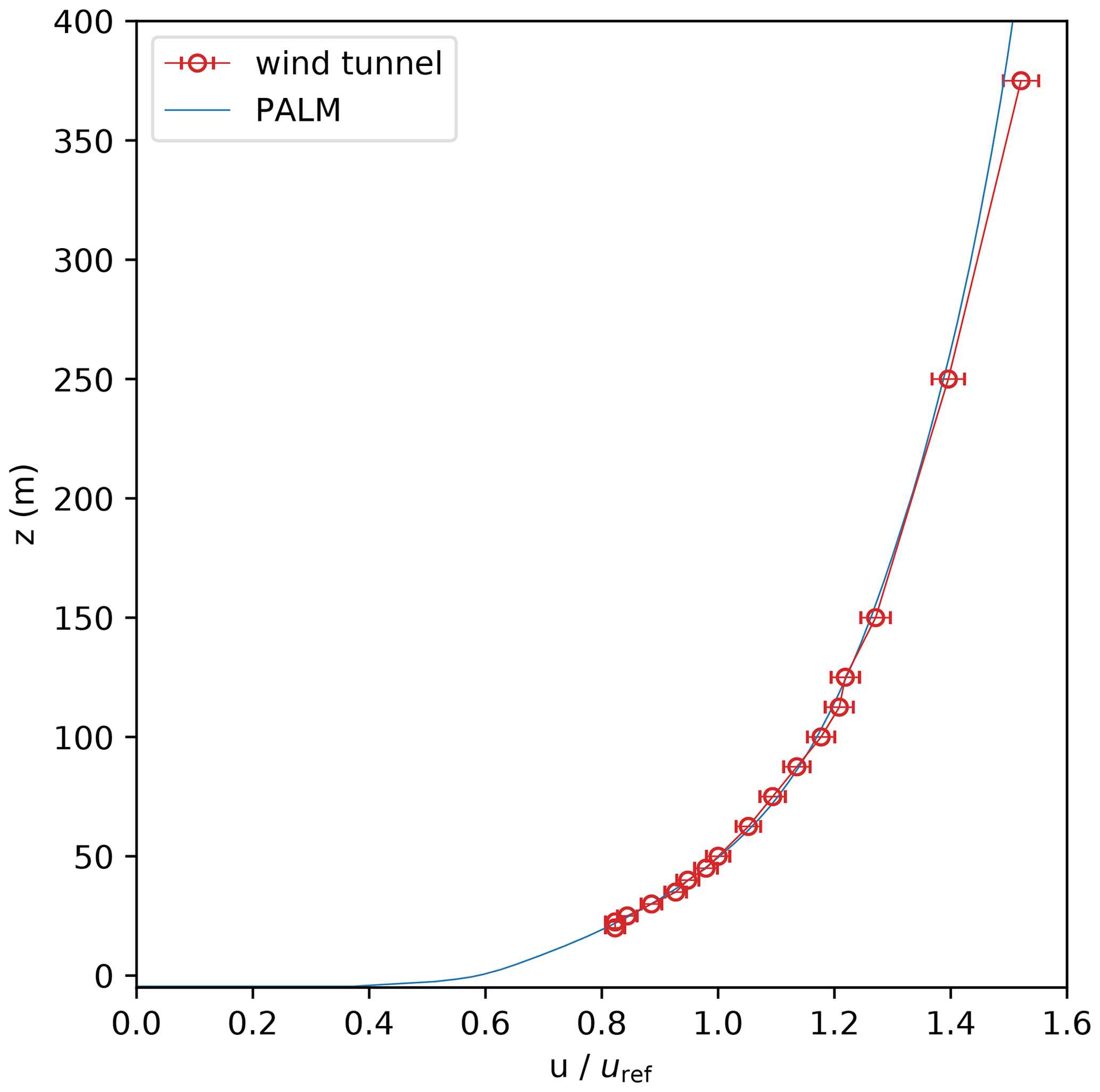
Figure 2Mean profiles of the approaching flow for the wind-tunnel experiment and the PALM simulation normalized with the reference velocity . Note that z=0 m is defined at street-level height while the lowest level within both experiments was at m, which is the water-level height.
The miniature replica of the HafenCity, Hamburg, Germany, has a scale of and represents an area of 2.6 km2 (see Fig. 1). Standard quality measurements during the wind-tunnel experiment proved scale-independence of the results (based on Townsend's hypothesis of self similarity) and allowed scaling of the results from model scale (ms) to full scale (fs). Scaling of space l, time t, and velocity u is achieved via
We used a two-dimensional laser doppler anemometry (LDA) system to measure component-resolved flow data at sampling rates of 200–800 Hz (model scale). This measurement method resolves even small-scale turbulence in time at most measurement locations. We recorded a 3 min time series at each measurement location, which corresponds to a period of about 25 h at full scale. Prandtl tubes continuously monitored the reference wind speed close to the tunnel inlet. For the model evaluation case presented here, measurements were taken at 25 different locations within the building setup as shown in Fig. 3. As the measurements were originally planned and used for a different study focusing on near-ground ventilation and pedestrian wind comfort, locations were not specifically chosen for the present study. However, the measurements still cover a variety of aspects of the flow within the building canopy including open areas, narrow and wide street canyons, and intersections.
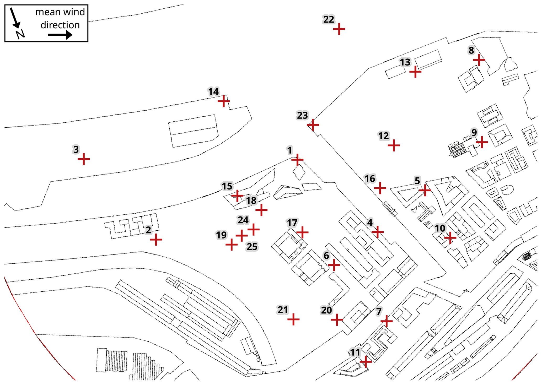
Figure 3Building layout used in the wind-tunnel experiment. Measurement locations are marked and labelled by their respective number.
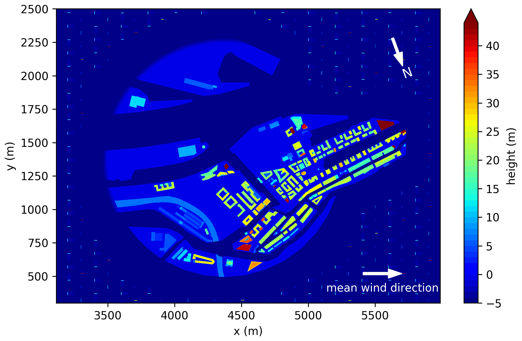
Figure 4Building layout and heights as used in the PALM simulation. The x direction is oriented to follow the mean wind direction. The total domain size is 6000, 2880, and 601 m in the x, y, and z direction, respectively. Note that z=0 m is defined at street-level height while the lowest level within both experiments was at m, which is the water-level height.
2.2 PALM simulation
We used the PALM Model System 6.0, revision 3921, to conduct the simulation for this study. We operated PALM using a fifth-order advection scheme after Wicker and Skamarock (2002) in combination with a third-order Runge–Kutta time-stepping scheme after Williamson (1980). Maronga et al. (2015, 2020a) provide a detailed description of the PALM model. We conducted the simulation at full scale with a domain size of 6000 m by 2880 m horizontally and 601 m vertically at a spatial resolution of m in each direction. This domain resulted in approximately 10.4×10⁹ grid points in our staggered Arakawa C-grid (Harlow and Welch, 1965; Arakawa and Lamb, 1977). The study region, i.e. the HafenCity area, was situated downstream of the simulation domain. We aligned the mean flow direction with the x direction. Hence, we rotated the model domain counter clockwise by 200∘ to produce a mean wind direction of 110∘.
Figure 4 displays the building layout used in PALM. PALM uses the mask method (Briscolini and Santangelo, 1989) for topography, where a grid volume is either 100 % fluid or 100 % obstacle. In combination with PALM's rectilinear grid, this method can cause non-grid aligned buildings to have inconsistent geometries (step-like) when compared with the wind-tunnel replica.
We based the setup for this study on the settings used by Letzel et al. (2012). A heterogeneous building setup usually requires a non-cyclic boundary condition along the mean flow direction to ensure that building-induced turbulence is not recycled into the analysis area. However, tests with non-cyclic boundary conditions along the mean flow showed that simulations would require extremely long simulation times to generate a stationary state. Hence, we used cyclic boundary conditions instead, which reduced the required CPU time significantly. We extended the domain in mean flow direction (x direction) to allow the building-induced turbulence to dissipate before the flow hits the target area again due to the cyclic conditions. Because we simulated an ideal, neutrally stratified case that neglected trace gases and the like within the city area, there was no disadvantage to use cyclic boundary conditions. After a simulation time of 1.5 h, the simulation reached a steady state.
We assumed a constant flux layer between the surface and the first computational grid level to calculate the surface shear stress. The exact value of the roughness length, z0, for the building surfaces is not known from the wind-tunnel experiment. Therefore, it was estimated as z0=0.01 m. This value was recommended by Basu and Lacser (2017) who state that . Due to the staggered grid, the first computational level was positioned 0.5Δz above the surface. Hence, m.
The estimated roughness length of the approaching flow in the wind-tunnel experiment was m (see Sect. 2.1). Surface-flux parameterizations cannot represent such a large roughness length at the simulated resolution (1 m). Therefore, we explicitly resolved the roughness using roughness elements of the exact same shape and layout as those elements used in the wind-tunnel experiment. This methodology produced a boundary layer flow in the simulation similar to that observed in the wind-tunnel experiment (see Fig. 2).
To match the conditions within the wind tunnel, we considered a strictly neutral atmosphere with potential temperature being constant over time. We also neglected the Coriolis force.
Munters et al. (2016) reported persistent streak-like artefacts in the flow field that are oriented along the mean wind direction for LES of neutral flows using cyclic boundary conditions. Such streaks naturally develop within the neutral boundary layer, reach lengths of several kilometres, and move along the mean wind direction while remaining stationary in the span-wise direction. These streaks form randomly and have a limited lifetime. In combination with cyclic boundary conditions, however, the start and end of a streak can merge, forming an infinite streak that is self-containing and persistent in time. To avoid the artificial persistence of these structures by cyclic boundary conditions, we use the shifting method of Munters et al. (2016). This method breaks up the infinite and persistent streak-like artefacts and ensures a natural dissipation. We shifted the flow by 300 m in the y direction, i.e. perpendicular to the mean wind direction, before entering the domain at the left boundary.
The wind field initializes with a turbulent wind field from a precursor simulation via the cyclic-fill method (Maronga et al., 2015). The setup of the precursor simulation was similar to the main simulation but with a reduced domain size of 600 m by 600 m in the horizontal direction. To initialize the precursor simulation, we measured the normalized approaching wind profile in the wind tunnel and scaled the wind speed to 4 m s−1 at 50 m height to obtain a representative wind speed for within the canopy layer. The fixed wind speed was 6.26 m s−1 at the top boundary for the precursor and main simulation.
The total simulation time of the main simulation was 4 h. The simulation achieved a steady state after the first 1.5 h. We used the results from the final 2.5 h for the analysis presented here (see Sect. 3).
Figure 2 shows the mean wind profile of the flow approaching the building area during the analysis time as well as the approaching flow of the wind-tunnel experiment. Note that we defined the street-level height at z=0 m and the lowermost height at water level, which is 5 m below street level (see Fig. 4). Hence, the approaching wind profile shown in Fig. 2 starts at m.
2.3 Measurement stations
Within the wind-tunnel experiment, wind speed was measured at certain measurement stations within the building array. Figure 3 shows the locations of the measurement stations. To be able to mirror the measurements as best as possible, we used the virtual measurement module of PALM (Maronga et al., 2020a). This module defines several virtual measurement stations within the model domain via geographical coordinates. The model domain must be geo-referenced in order to identify the grid points closest to the measurement location. PALM references the geographical coordinates based on the coordinates of the lower left corner of the domain and the domain's orientation.
When mapping the measurement stations onto the PALM grid, there were two difficulties. First, there was not always a grid point available at the exact location of the measurement within the wind-tunnel experiment. Therefore, measurement positions can differ between the virtual and wind-tunnel measurements by a distance of less than 1 m. Second, the topography in the vicinity of a measurement point at the virtual stations may differ from the wind-tunnel stations due to the topography representation used in PALM (see Sect. 2.2). To overcome these two issues, we also recorded virtual measurements from the grid points neighbouring a measurement position. In post-processing, we analysed the area of each measurement station and selected the measurement from the grid point that best fit the wind-tunnel measurements. Each measurement station recorded vertical profiles with a sampling rate between 8.7 and 11.2 Hz (measurements recorded during each time step).
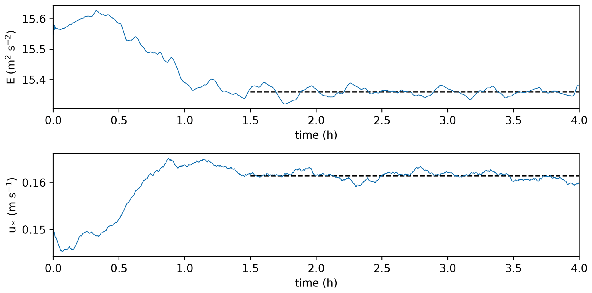
Figure 5Time series of the total kinetic energy E and the friction velocity u* of the PALM simulation.
3.1 PALM simulation
The PALM simulation required a spin-up time of 1.5 h, which is evident by the time series of the domain-averaged kinetic energy and the friction velocity u* (see Fig. 5). Both quantities stabilized after 1.5 h at approximately E=15.4 m2 s−2 and m s−1. Therefore, we only evaluated data from the last 2.5 h of the simulation.
Figure 6 shows the horizontally and time-averaged vertical profile of the stream-wise component of the vertical momentum flux wu. The vertical momentum flux wu is split into a resolved component and a sub-grid scale (SGS) component. An SGS model parameterizes the SGS component. The less the SGS model contributes to the flux the better resolved is the turbulence causing the flux. The ratio of the resolved and the total momentum flux is close to 1 revealing that the simulation domain properly resolved the turbulence (see Fig. 6).
Turbulent structures tend to become smaller the closer they get to the surface. Hence, at the surface, the constant grid spacing resolves less turbulence (Maronga et al., 2020b). However, the ratio between resolved and total wu exceeds 0.9 except for the lowest two grid levels where the ratio reduces to 0.78. The discontinuity at z=15 m is related to the roughness elements. Most of these elements extend to z=15 m, causing the disturbance in the vertical wu profile at that height.
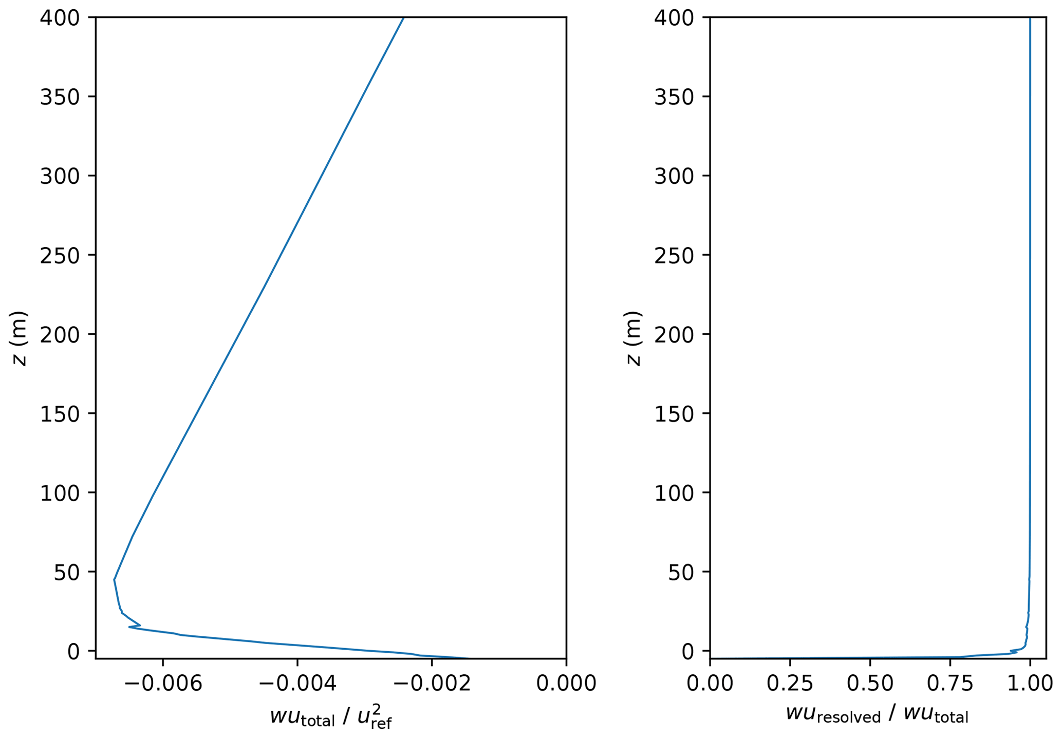
Figure 6Mean profile of the vertical momentum flux and the ratio between resolved and total flux, averaged over the entire domain of the PALM simulation. Please note the two different horizontal scales for momentum flux (bottom scale) and flux ratio (top scale).
To visualize the turbulent structures, Fig. 7 shows a snapshot of the magnitude of the three-dimensional vorticity as a proxy for turbulence. Strong turbulence (yellow and red structures) occurs in the vicinity of buildings, while weak turbulence occurs above smooth surfaces. Roughness elements that are not visible within Fig. 7 cause the strong turbulence outside of the building array.
3.2 Comparison between wind tunnel and PALM
To compare the simulation and the wind-tunnel experiment, we must first normalize the results as the simulation and wind-tunnel experiment were conducted on different scales and mean wind speeds. The reference wind speed uref used for normalization corresponds to the wind speed of the approaching flow at a height of 50 m (full scale). Previously conducted laboratory experiments defined the reference height to be representative of the measured canopy flow. The reference height falls within the range expected to most accurately model a scaled neutrally stratified atmospheric boundary layer wind flow. We report our results at full scale unless otherwise stated.
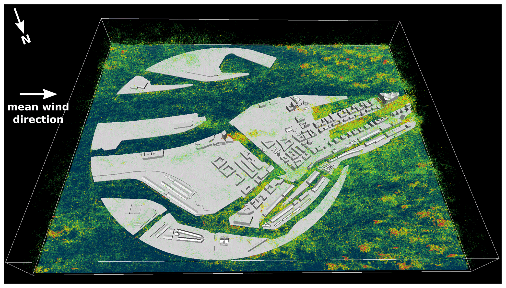
Figure 7View of the volume-rendered instantaneous turbulence structures above the building array. Turbulence is visualized using the magnitude of the three-dimensional vorticity. Green and red indicate low and high values, respectively. The image was rendered using VAPOR (Li et al., 2019, http://www.vapor.ucar.edu/, last access: 2 June 2021) and the background image was designed by freepic.diller/Freepik (http://www.freepik.com, last access: 16 May 2019).
Figure 8 shows the wind distribution for each measurement station at the lowest measurement height for (a) the wind-tunnel measurements (z=3 m) and (b) the PALM simulation (z=2.5 m). Due to the staggered grid used in PALM (see Sect. 2.2), the positions of the PALM measurements are 0.5 m below their corresponding wind-tunnel measurements. Note that measurement station 15 stands on top of a building where measurements were only available above 18 m height (see Fig. 3). At most measurement stations, the main wind direction in the PALM simulation is similar to the wind-tunnel data. Noticeable differences in the distribution of wind directions occur at stations 6, 7, 10, and 20, where the PALM simulation reports a larger variation in wind direction or a different mean wind direction. On average, the wind speed is 9 % less in the PALM simulation than in the wind-tunnel measurements.
At 10 m height (PALM: 9.5 m), the wind distributions are still very close between PALM and the wind tunnel at most stations (see Fig. 9). Stations 6, 10, and 20 still show noticeable differences. The difference in average wind speed reduces to 5 % between PALM and wind-tunnel results. At 40 m height and above, the difference reduces to less than 2.5 %.
Figure 10 shows scatter plots of wind-tunnel and PALM measurements at each station and height, which are 173 data pairs in total. Looking at the horizontal wind speed Uhor and the wind-speed components u and v, PALM underestimates the lower values while higher values compare well to the wind-tunnel measurements. Wind direction d differs by less than 4∘ on average with a maximum difference of less than 44∘. It has to be noted, however, that wind-tunnel measurements might be located between grid points of the PALM grid creating a spatial offset between the measurements. Especially close to obstacles, this spatial offset can lead to differences between both experiments.

Figure 8Wind-speed distribution (wind rose plots) at all measurement stations for (a) wind-tunnel measurements and (b) the PALM simulation at about 3 m height above street level (wind tunnel: 3 m, PALM: 2.5 m). Axes are only shown for a single station for better overview, but all wind distributions are scaled equal. Numbers indicate the station number.
Three major reasons caused the general lower wind speeds in the PALM simulation: (i) a mismatch in measurement height, (ii) a mismatch in z0 between both experiments, and (iii) the stepwise building representation caused by PALM's rectilinear grid. The staggered Arakawa C-grid caused the PALM measurements to be located 0.5 m below the corresponding wind-tunnel measurements. PALM calculates u and v at half the height of each grid cell. With a grid size of Δz=1 m, u and v are, hence, calculated at heights of 0.5, 1.5, 2.5 m, etc. We chose to not interpolate between the height levels in order to not alter the simulation results by adding additional uncertainty due to the chosen interpolation techniques. When comparing PALM results at 0.5 m above the wind-tunnel measurements, the underestimation of wind-speed reduces to 5 % at 3 m height. Because vertical gradients of the wind-speed decrease with height, differences in measurement heights are less severe at greater heights.
Second, a mismatch of z0 between both experiments also affects results most significantly at the lowest height levels. This is supported by the fact that we observed the largest difference in mean wind speed (9 % lower wind speed) at the lowest measurement height. Hence, the surfaces in the wind-tunnel experiment might have been smoother than estimated and z0=0.01 m might have been too large. In a different not yet published wind-tunnel experiment with similar wall materials of the building model, we observed roughness lengths between 0.002 and 0.01 m. This puts the chosen z0 for the simulation at the upper end of the possible value range for the roughness within the wind-tunnel experiment.
The third reason, the stepwise building representation, affects results within the entire building canopy layer. Because PALM discretizes obstacles on a rectilinear grid as mentioned in Sect. 2.2, smooth building walls are represented by stepwise surfaces if not aligned with the grid layout. Therefore, building walls become significantly rougher than they were in the wind-tunnel experiment. This causes higher turbulence and an overall reduced mean wind speed within the building canopy layer.
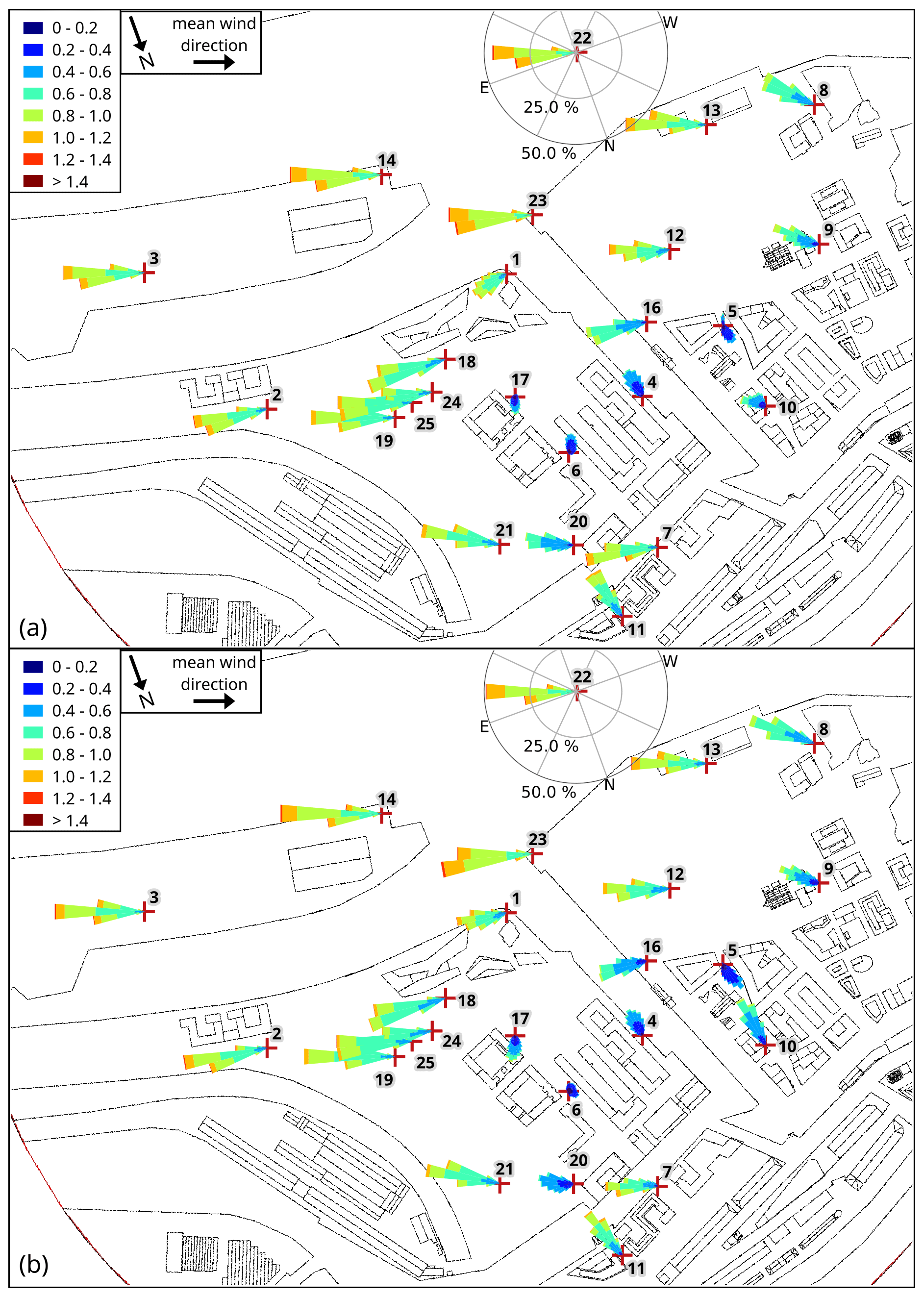
Figure 9Wind-speed distribution (wind rose plots) at all measurement stations for (a) wind-tunnel measurements and (b) the PALM simulation at about 10 m height above street level (wind tunnel: 10 m, PALM: 9.5 m). Axes are only shown for a single station for better overview, but all wind distributions are scaled equal. Numbers indicate the station number.
To better evaluate the deviations between both experiments, we calculated different validation metrics. COST Action 732 (Schatzmann et al., 2010) lists several validation metrics to help evaluate simulation models. The proposed metrics are the factor of two FAC2, the hit rate q, the fractional bias FB, the geometric mean bias MG, the normalized mean square error NMSE, and the geometric variance VG. Additionally, we calculated the correlation coefficient R. These metrics are defined as
with Oi being the observed (wind tunnel), Pi the predicted (PALM) measurements, δr the relative deviation threshold, δa the absolute deviation threshold, and N the total number of measurements; the overline denotes an average over all measurements and σP and σO are the standard deviation of P and O, respectively. We set the deviation thresholds to δr=0.25 for all variables as recommended by VDI (2005). Table 1 lists the δa used for all variables.
Table 1Calculated validation metrics for different variables. The rightmost column gives the respective value of a perfect match between simulation and observation.
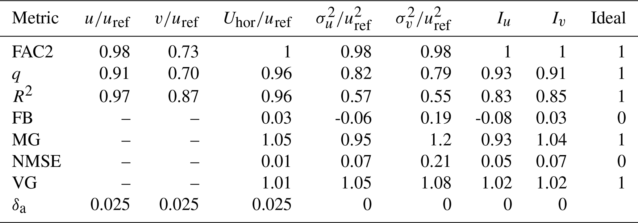
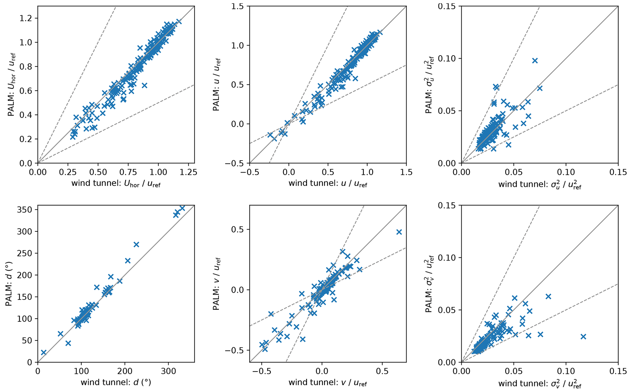
Figure 10Scatter plots of wind tunnel and PALM measurements of horizontal wind speed Uhor, wind direction d, wind-velocity components u and v, and their variance and for all 25 measurement stations and all heights (173 data pairs in total). Solid lines indicate perfect agreement and dashed lines indicate the area between a deviation factor of 0.5 and 2.
We calculated the validation metrics for the horizontal wind speed Uhor, the wind-velocity components u and v, their variance and , as well as for the turbulence intensities Iu and Iv that are defined as the standard deviation divided by the mean horizontal wind speed (see Table 1). In general, all validation metrics are close to their ideal values indicating a high agreement between both experiments. The largest deviation between both experiments is apparent for v where both FAC2 and q give the lowest values. However, q is still within the acceptable range of q≥0.66, defined by VDI (2005). The metrics also reflect the abovementioned findings that PALM underestimates the mean wind speed. Both FB and MG indicate an underestimation of approximately 5 % (MG=1.05). The metrics also indicate an underestimation of σv of 20 % (MG=1.2), which is visible in Fig. 10. However, all metrics lie well within the margins reported by Hanna et al. (2004) for an acceptable performing model. These margins are FAC2>0.5, , , NMSE<4, and VG<1.6.
Hertwig et al. (2017) recommend to evaluate the shape parameters of the wind speed distributions of u and v when comparing LES and wind-tunnel results. Figure 11 shows the skewness γ and the excess kurtosis β of u and v. Between both experiments, γu mostly agrees and shows either symmetrical distributions (γu≈0) or a positive skew. For v, distributions tend to have a lower skewness in PALM than in the wind-tunnel measurements. Also, βv is smaller meaning that the distributions are less peaked. This is also related to the higher roughness in the PALM simulation because this produces a wider spread of the distribution with a less pronounced peak, resulting in lower β and (in case of a positive average as is the case here) γ. Again, this is more pronounced in the span-wise wind component v.
The higher roughness and enhanced turbulence lead to a less correlated flow and reduced length scales. Figure 12 displays the comparison of length scales Lu and Lv of the u and v component, respectively. We calculated the length scales based on the integral timescale T:
where T is calculated using the auto-correlation function Ra:
with tl being the time lag.
Most striking are the considerably lower values of Lv within the PALM simulation. However, most data points still lie within the factor-of-two margins: FAC2(Lv)=0.8. PALM tends to underestimate low Lu and overestimate Lv.
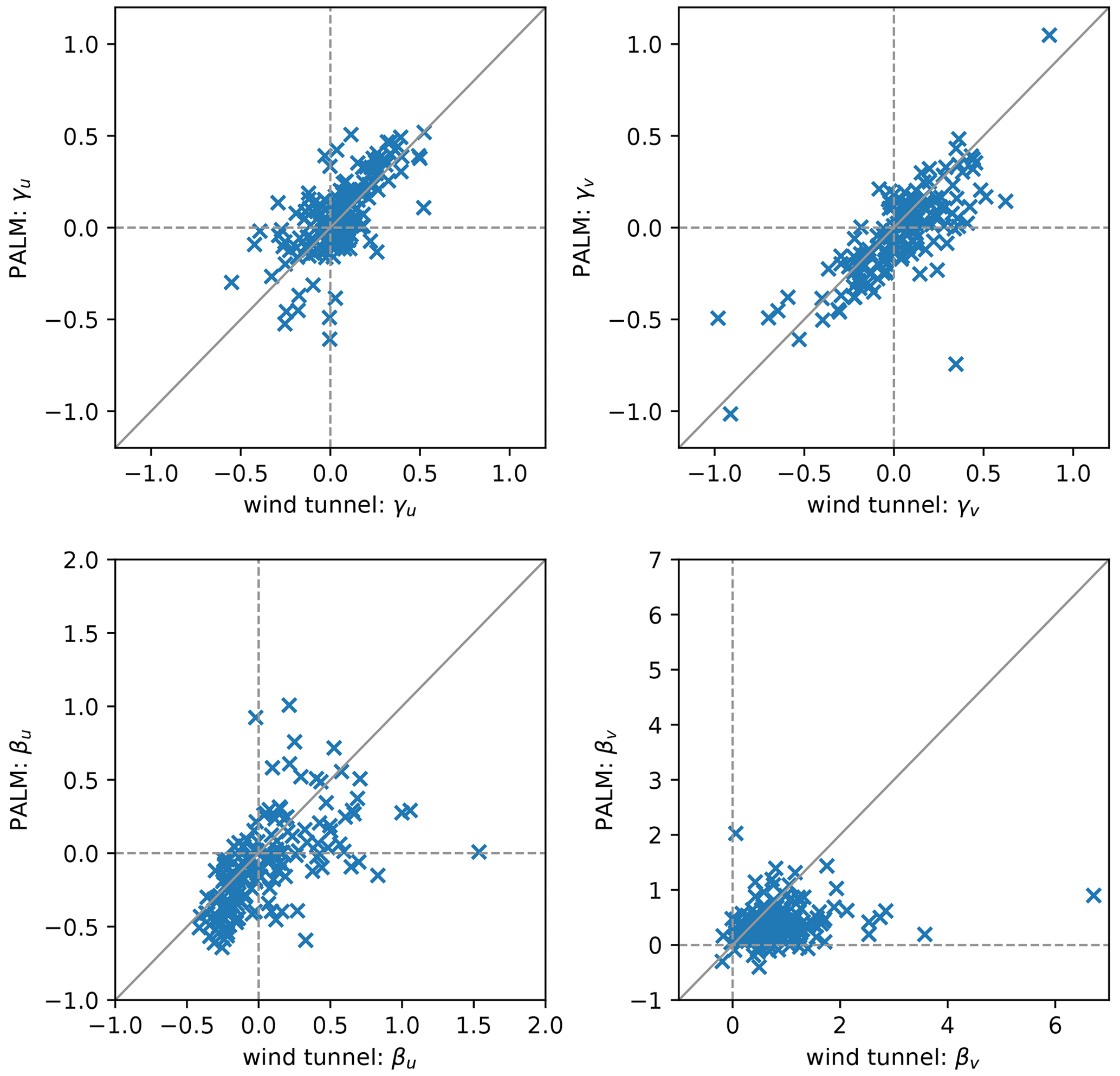
Figure 11Scatter plots of wind tunnel and PALM measurements of skewness γ and excess kurtosis β of the horizontal wind velocity components for all 25 measurement stations and all heights (173 data pairs in total). Solid lines indicate perfect agreement.
In the following, we compare the vertical profiles recorded at the measurement stations. Because many vertical profiles showed nearly identical behaviour at different stations, we limit the discussion to three stations: 4, 11, and 7. We chose these stations as examples of a good, an average, and a relatively poor agreement, respectively, between the simulation and the wind-tunnel measurements.
Figure 13 shows vertical profiles of Uhor, d, u, and v, as well as turbulence intensity I, skewness γ, excess kurtosis β, and length scale L for u and v measured at station 7. Error bars show the standard deviation of u and v. The blue shaded area shows the range of values of the neighbouring grid points within PALM at the respective measurement station.
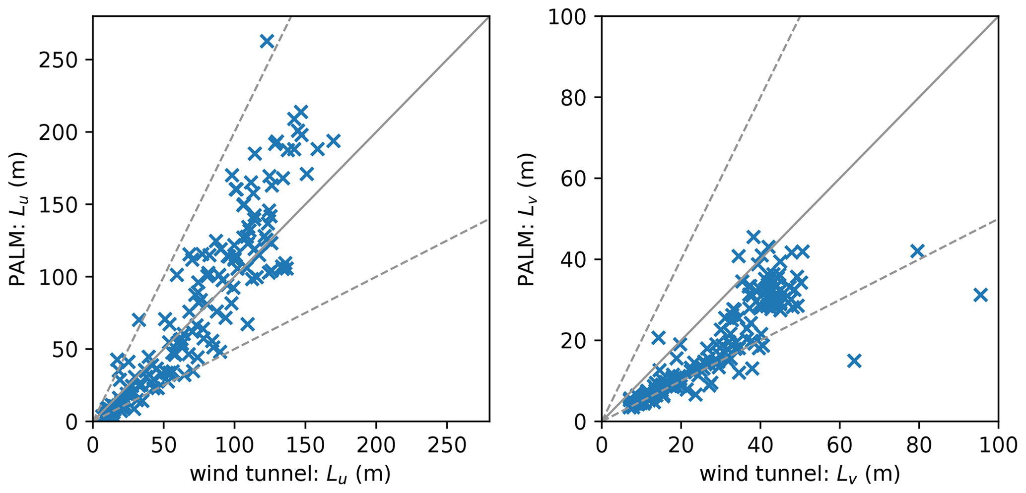
Figure 12Scatter plots of wind tunnel and PALM measurements of the length scales Lu and Lv of the velocity components u and v, respectively, for all 25 measurement stations and all heights (173 data pairs in total). Solid lines indicate perfect agreement and dashed lines indicate the area between a deviation factor of 0.5 and 2.

Figure 13Profiles of mean horizontal wind speed Uhor, wind direction d, and wind components u and v as well as turbulence intensity I, skewness γ, excess kurtosis β, and length scale L of both wind velocity components u and v at measurement station 7. Error bars denote the standard deviation of the respective quantity. Note that z=0 denotes street-level height.
Station 7 is situated at the opening of a street canyon within the lee of a building edge (see Fig. 3). Because the surrounding building walls were not aligned with the PALM grid, the building edge had a different shape within the simulation than in the wind-tunnel experiment. This shape difference created an enlarged corner vortex in the simulation. The vortex increased the turbulence and decreased the mean wind speed at station 7 compared to the wind-tunnel results, as shown in Fig. 13. Also, d is affected and deviates from the wind-tunnel results. The effect of rougher building walls by the stepwise representation is limited to the canopy layer. Therefore, d, Iu, and Iv agree significantly better with the wind-tunnel measurements above the rooftop height that is situated between 26 and 36 m in the vicinity of station 7. Due to higher turbulence below the rooftop level, βv decreases, indicating a less peaked distribution, while the lower γu indicates larger tails towards low u values. The higher turbulence also causes L to be shorter within the canopy. Above the canopy layer, the mean wind speed and length scales are larger than in the wind-tunnel experiment because of a higher vertical momentum flux in the simulation caused by the higher roughness within the canopy layer. Similar behaviour can be found at station 20 (profiles not shown), which is located close to a windward building corner. In this case, the blocking effect of the building is increased because of the broader building edge, causing significant differences in wind-direction distribution and mean wind speed (see Figs. 8 and 9).
Profiles not affected by corner flows or the blocking effect tend to agree better between PALM and wind-tunnel measurements. Station 11, positioned at the centre of a street canyon (see Fig. 3), serves as an example of such a measurement location. Profiles tend to agree significantly better within the canopy layer than for station 7, as shown in Fig. 14. Higher deviations between the experiments appear close to the rooftop height (between 26 and 36 m). The roofs of the surrounding buildings have small structures that might not be sufficiently resolved. Hence, the details of the building layout differ between the simulation and the wind tunnel at station 11. Stations 5, 6, 10, and 17 show results similar to those of station 11. Figure 14 shows a large value range of the profiles as indicated by the blue-shaded areas. This large range shows that profiles vary significantly inside the street canyon depending on the distance to the building walls. Hence, it is very important to place the measurements correctly in the simulation if they are situated in close vicinity to buildings.

Figure 14Profiles of mean horizontal wind speed Uhor, wind direction d, and wind components u and v as well as turbulence intensity I, skewness γ, excess kurtosis β, and length scale L of both wind velocity components u and v at measurement station 11. Error bars denote the standard deviation of the respective quantity. Note that z=0 denotes street-level height.
Station 4 is located at the leeward site of a flat-roofed building (see Fig. 3). Also, no building corners that could produce blocking effects or corner flows are within the proximity of station 4. Profiles at station 4, displayed in Fig. 15, show only small deviations between the two experiments. The rougher wall, generated by the building representation, produces larger turbulence and a less peaked distribution of u and v within the canopy layer. However, results agree significantly better at station 4 compared to station 7 and 11. Hence, PALM reproduces the wind field better if the building structures are less complex.
Figure 16 shows the spectral energy density S measured at station 4 (left panel) and station 11 (right panel) at the profile top, rooftop, and near the surface (top, centre, and bottom row, respectively). Spectra measured at station 7 are comparable to those of station 11 and are therefore not shown. The covered range of frequencies f differ between PALM and wind-tunnel measurements because the sampling rate of the measurements and the measured time interval vary between the PALM and the wind-tunnel experiment. However, results of both experiments overlap over a large range of frequencies.
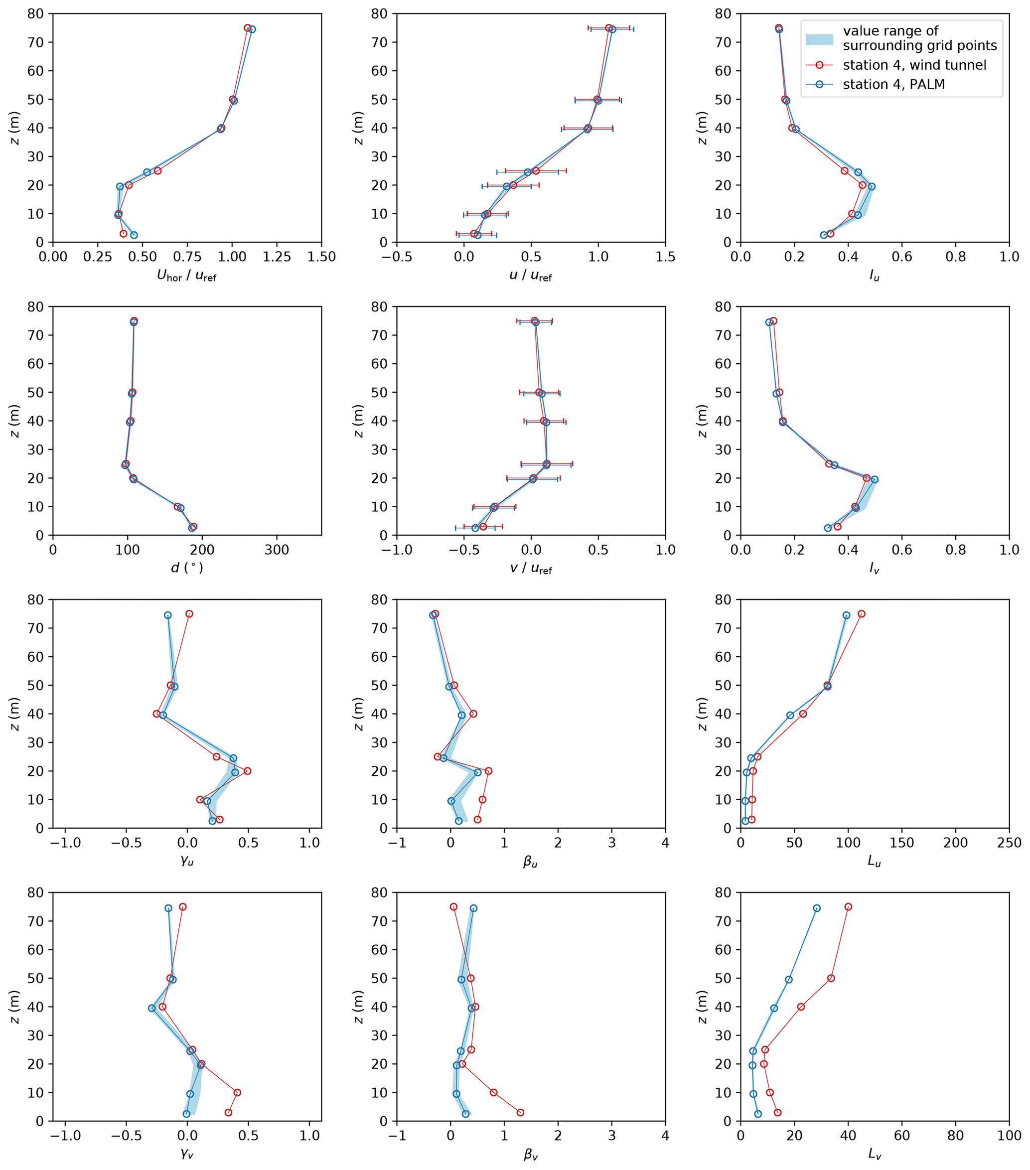
Figure 15Profiles of mean horizontal wind speed Uhor, wind direction d, and wind components u and v as well as turbulence intensity I, skewness γ, excess kurtosis β, and length scale L of both wind velocity components u and v at measurement station 4. Error bars denote the standard deviation of the respective quantity. Note that z=0 denotes street-level height.
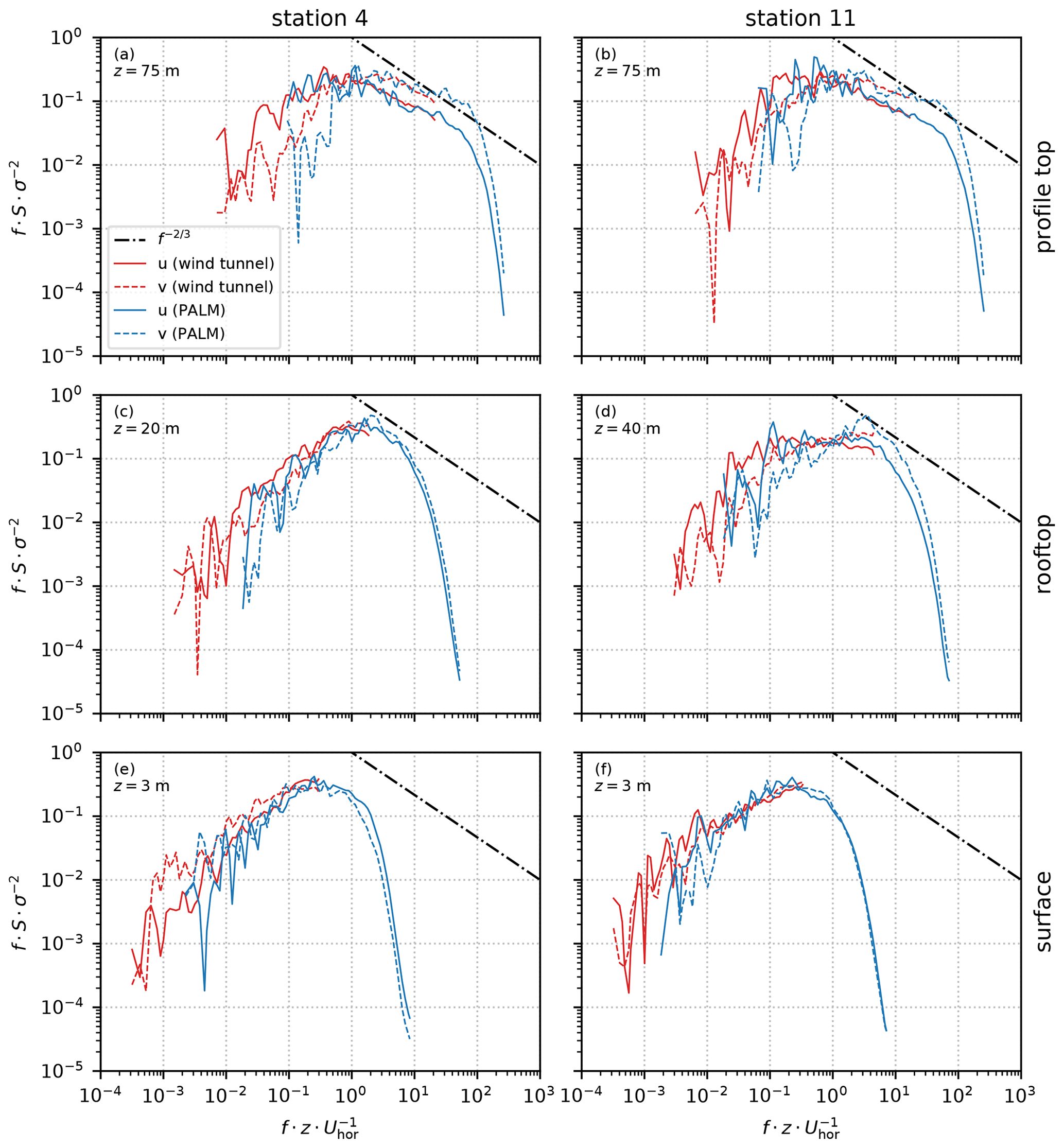
Figure 16Spectral energy density S for u and v at station 4 (a, c, e) and station 11 (b, d, f) at profile top (a, b), rooftop height (c, d), and near the surface (e, f). S is normalized by multiplying by the frequency f and dividing by the variance σ2. For reference, the dash-dotted line shows a slope f−⅔ indicating the slope of energy decay according to Kolmogorov's theory. Note that z is given relative to street-level height.
The spectra of u and v coincide to a high degree between the simulation and the wind-tunnel measurements at all heights. At both stations, the spectra show an exponential decrease between and 50 at 75 m height (above the canopy layer), indicating the inertial range (Fig. 16a and b). The normalized energy spectrum decays with roughly following Kolmogorov's theory. At high frequencies, spectra of the PALM measurements rapidly decay, which is related to numerical dissipation. This decay is a typical behaviour of LES models using high-order differencing schemes (e.g. Glendening and Haack, 2001; Kitamura and Nishizawa, 2019).
At rooftop height (Fig. 16c and d), PALM's spectra are shifted towards higher frequencies compared to those of the wind tunnel at the same height. This shift indicates that PALM simulates smaller-scale turbulence at these heights. The shift can be related to higher roughness and further fosters the abovementioned findings from the profile analysis. The stepwise representation of the buildings introduces additional roughness causing smaller turbulence elements and, hence, a shift of the energy spectrum to higher frequencies. Station 4 shows a more pronounced shift than station 11, which might, however, be related to the more distinct maximum and, hence, better visibility of a shift at station 4.
The spectra agree better between PALM and the wind-tunnel measurements close to the surface. However, the wind-tunnel measurements did not cover the inertial range at 3 m height because of the limitation of the measurement frequency and small turbulent structures near the surface. PALM does not resolve the inertial range at this height as well because the turbulence elements are smaller than the grid size of 1 m; hence, the small-scale turbulence cannot be directly simulated. Comparing the measured spectra to the theoretical decay of f−⅔, the inertial range is indeed hardly represented within the data.
In this study, we analysed PALM's capability to simulate a complex flow field within a realistic urban building array. We compared simulation results to measurements done at the EWTL facility at the University of Hamburg, Germany. The aim was to evaluate the dynamic core of the newest version of PALM, which underwent significant code changes in recent model development.
The comparison of PALM results with the wind-tunnel data demonstrated that PALM is capable of accurately simulating a neutrally stratified urban boundary layer produced by a realistic, complex building array. We compared measurements from the simulation to those of the wind-tunnel experiment at several positions throughout the building array. These positions included non-obstructed locations, windward and leeward sides of buildings, street canyons, and roadway intersections. Overall, the PALM results displayed relatively good agreement with the corresponding wind-tunnel measurements in regards to wind speed and direction as well as turbulence intensity. Validation metrics proposed by Schatzmann et al. (2010) were all within the acceptable ranges.
However, PALM underestimates wind speed and overestimates turbulence close to the ground and building surfaces. Estimates differed most in the span-wise wind velocity component. Paas et al. (2020) recently reported such discrepancies when comparing PALM simulations to real-world measurements. These differences partly occur due to an overestimation of roughness mainly introduced by the stepwise representation of buildings onto PALM's rectilinear grid. This representation causes building walls not aligned with the grid to appear significantly rougher, resulting in lower wind speed and higher turbulence close to walls, especially in the vicinity of building corners. Also, the used roughness length of z0=0.01 m might be larger than the actual surface roughness in the wind-tunnel experiment, causing the highest difference of mean wind speed (9 %) at the lowest analysis height.
To a lesser degree, the mismatch in measurement height is responsible for a difference in mean wind speed. Due to PALM's staggered Arakawa C-grid, output was not available at the exact same position as in the wind-tunnel experiment but shifted half a grid spacing (0.5 m) downwards. This half-grid shift accounted for up to 3 % difference in wind speed at the lowest grid level.
If z0 is unknown, this can certainly produce differences between PALM and reference data close to surfaces. More importantly, however, is a good representation of building structures. If the focus lies on flow features in close vicinity to buildings, the most important buildings should align with the simulation grid. Also, we recommend a high grid resolution to represent structures as close to the reference as possible. To achieve this, future validations could utilize PALM's nesting feature in order to cope with increasing computational demand of reduced grid size (Hellsten et al., 2020). A higher resolution also reduces the errors introduced by shifting locations of measurements of PALM when comparing against reference data. These errors can otherwise cause deviations close to buildings, where large gradients can cause significant differences in results (see, e.g. the profiles of station 11; Fig. 14). In a future release of PALM, an immersed boundary condition will be available (e.g. Mittal and Iaccarino, 2005). This new boundary condition will mitigate the increased roughness effect introduced by the stepwise representation of building walls not aligned with the rectilinear grid.
Lastly, we provide some general advice for the setup preparation. In the present study, we experienced that input data must always be checked very carefully, especially large building data sets. These building setups might contain errors and false building heights or missing and/or displaced buildings, which are more difficult to spot than in setups with a limited number of buildings. This is, of course, of utmost importance for the area of interest. However, the upwind region also requires proper verification because it directly affects the analysis area. Additionally, when comparing with other experiments, like real-world or wind-tunnel measurements, the positioning of the measurements must be thoroughly checked, as mentioned by Paas et al. (2020). This is true for positioning virtual measurements within the PALM domain as well. At positions with complex wind fields, it can make a large difference for the results if measurement positions are off by only a single grid point. This of course depends on the grid spacing and will be most relevant when using relatively coarse grids.
This study focused on only a single, but the most essential, component of PALM, the dynamic core. However, a full validation of the entire model requires additional studies focusing on the other model components like the radiation module, the chemistry module, or the land surface module. Some of these are already validated (Resler et al., 2017; Kurppa et al., 2019; Fröhlich and Matzarakis, 2020; Gehrke et al., 2020). Others will follow in future publications.
The PALM model system is freely available from http://palm-model.org (last access: 2 June 2021) and distributed under the GNU General Public License v3 (http://www.gnu.org/copyleft/gpl.html, last access: 2 June 2021). The model source code of version 6.0 in revision 3921 as well as input data and measurement results presented in this paper are archived on the Research Data Repository of the Leibniz University Hannover (Gronemeier et al., 2020b), together with the plotting scripts to reproduce the presented figures (Gronemeier et al., 2020a).
BL and KS created the wind-tunnel setup. KS conducted the wind-tunnel measurements and analysis with supervision of FH and BL. TG, SR, and BM created the simulation setup. TG carried out the simulations and precursor test simulations with the supervision of SR. All authors took part in data analysis of the comparison. TG compiled the manuscript with contributions by all coauthors.
The authors declare that no competing interests are present.
We would like to thank everyone who helped conduct the experiments and write software for the analysis of the results (including data preparation, model building, and code debugging). We thank the two anonymous referees who helped to significantly improve the manuscript with their valuable comments. We thank Wieke Heldens and Julian Zeidler (German Aerospace Center, DLR) for their support during the project and especially for preparing the building data used within this study. We thank Christopher Mount (Leibniz University Hannover) for proofreading the manuscript.
This study was part of the [UC]2 project that is funded by the German Federal Ministry of Education and Research (BMBF). The study was conducted in collaboration with the two sub-projects MOSAIK and 3DO. All simulations were carried out on the computer clusters of the North-German Supercomputing Alliance (HLRN; https://www.hlrn.de/, last access: 2 June 2021). Data analysis was done using Python.
This research has been supported by the by the German Federal Ministry of Education and Research (BMBF) within the framework “Research for Sustainable Development” (FONA; https://www.fona.de/de/, last access: 2 June 2021; grant nos.
01LP1601 and 01LP1602).
The publication of this article was funded by the open-access fund of Leibniz Universität Hannover.
This paper was edited by Simon Unterstrasser and reviewed by two anonymous referees.
Arakawa, A. and Lamb, V. R.: Computational Design of the Basic Dynamical Processes of the UCLA General Circulation Model, in: General Circulation Models of the Atmosphere, vol. 17, edited by: Chang, J., Methods in computational Physics, 173–265, 1977. a
Basu, S. and Lacser, A.: A Cautionary Note on the Use of Monin–Obukhov Similarity Theory in Very High-Resolution Large-Eddy Simulations, Bound.-Lay. Meteorol., 163, 351–355, https://doi.org/10.1007/s10546-016-0225-y, 2017. a
Blocken, B., Carmeliet, J., and Stathopoulos, T.: CFD Evaluation of Wind Speed Conditions in Passages between Parallel Buildings – Effect of Wall-Function Roughness Modifications for the Atmospheric Boundary Layer Flow, J. Wind Eng. Ind. Aerod., 95, 941–962, https://doi.org/10.1016/j.jweia.2007.01.013, 2007. a
Briscolini, M. and Santangelo, P.: Development of the Mask Method for Incompressible Unsteady Flows, J. Comp. Phys., 84, 57–75, https://doi.org/10.1016/0021-9991(89)90181-2, 1989. a
Fröhlich, D. and Matzarakis, A.: Calculating human thermal comfort and thermal stress in the PALM model system 6.0, Geosci. Model Dev., 13, 3055–3065, https://doi.org/10.5194/gmd-13-3055-2020, 2020. a
Gehrke, K. F., Sühring, M., and Maronga, B.: Modeling of land-surface interactions in the PALM model system 6.0: Land surface model description, first evaluation, and sensitivity to model parameters, Geosci. Model Dev. Discuss. [preprint], https://doi.org/10.5194/gmd-2020-197, in review, 2020. a
Glendening, J. W. and Haack, T.: Influence Of Advection Differencing Error Upon Large-Eddy Simulation Accuracy, Bound.-Lay. Meteorol., 98, 127–153, https://doi.org/10.1023/A:1018734205850, 2001. a
Gronemeier, T. and Sühring, M.: On the Effects of Lateral Openings on Courtyard Ventilation and Pollution – A Large-Eddy Simulation Study, Atmosphere, 10, 63, https://doi.org/10.3390/atmos10020063, 2019. a
Gronemeier, T., Surm, K., Harms, F., Leitl, B., Maronga, B., and Raasch, S.: Dataset: Evaluation of the Dynamic Core of the PALM Model System 6.0 in a Neutrally Stratified Urban Environment: Simulation Input Data and Measurement Data, Leibniz Universität Hannover, https://doi.org/10.25835/0015082, 2020a. a
Gronemeier, T. et al.: Dataset: PALM 6.0 r3921, Leibniz Universität Hannover, https://doi.org/10.25835/0046914, 2020b. a
Hanna, S. R., Hansen, O. R., and Dharmavaram, S.: FLACS CFD Air Quality Model Performance Evaluation with Kit Fox, MUST, Prairie Grass, and EMU Observations, Atmos. Environ., 38, 4675–4687, https://doi.org/10.1016/j.atmosenv.2004.05.041, 2004. a
Harlow, F. H. and Welch, J. E.: Numerical Calculation of Time-Dependent Viscous Incompressible Flow of Fluid with Free Surface, Phys. Fluids, 8, 2182, https://doi.org/10.1063/1.1761178, 1965. a
Hellsten, A., Ketelsen, K., Sühring, M., Auvinen, M., Maronga, B., Knigge, C., Barmpas, F., Tsegas, G., Moussiopoulos, N., and Raasch, S.: A Nested Multi-Scale System Implemented in the Large-Eddy Simulation Model PALM model system 6.0, Geosci. Model Dev. Discuss. [preprint], https://doi.org/10.5194/gmd-2020-222, in review, 2020. a
Hertwig, D., Patnaik, G., and Leitl, B.: LES Validation of Urban Flow, Part I: Flow Statistics and Frequency Distributions, Environ. Fluid Mech., 17, 521–550, https://doi.org/10.1007/s10652-016-9507-7, 2017. a
Kanda, M., Inagaki, A., Miyamoto, T., Gryschka, M., and Raasch, S.: A New Aerodynamic Parametrization for Real Urban Surfaces, Bound.-Lay. Meteorol., 148, 357–377, https://doi.org/10.1007/s10546-013-9818-x, 2013. a
Kitamura, Y. and Nishizawa, S.: Estimation of Energy Dissipation Caused by Odd Order Difference Schemes for an Unstable Planetary Boundary Layer, Atmos. Sci. Lett., 20, e905, https://doi.org/10.1002/asl.905, 2019. a
Kurppa, M., Hellsten, A., Auvinen, M., Raasch, S., Vesala, T., and Järvi, L.: Ventilation and Air Quality in City Blocks Using Large-Eddy Simulation – Urban Planning Perspective, Atmosphere, 9, 65, https://doi.org/10.3390/atmos9020065, 2018. a
Kurppa, M., Hellsten, A., Roldin, P., Kokkola, H., Tonttila, J., Auvinen, M., Kent, C., Kumar, P., Maronga, B., and Järvi, L.: Implementation of the sectional aerosol module SALSA2.0 into the PALM model system 6.0: model development and first evaluation, Geosci. Model Dev., 12, 1403–1422, https://doi.org/10.5194/gmd-12-1403-2019, 2019. a
Leitl, B. and Schatzmann, M.: Validation Data for Urban Flow and Dispersion Models – Are Wind Tunnel Data Qualified?, in: Fifth International Symposium on Computational Wind Engineering (CWE2010), Chapel Hill, North Carolina, USA, 23–27 May 2010, p. 8, 2010. a
Letzel, M. O., Krane, M., and Raasch, S.: High Resolution Urban Large-Eddy Simulation Studies from Street Canyon to Neighbourhood Scale, Atmos. Environ., 42, 8770–8784, https://doi.org/10.1016/j.atmosenv.2008.08.001, 2008. a, b
Letzel, M. O., Helmke, C., Ng, E., An, X., Lai, A., and Raasch, S.: LES Case Study on Pedestrian Level Ventilation in Two Neighbourhoods in Hong Kong, Meteorol. Z., 21, 575–589, https://doi.org/10.1127/0941-2948/2012/0356, 2012. a
Li, S., Jaroszynski, S., Pearse, S., Orf, L., and Clyne, J.: VAPOR: A Visualization Package Tailored to Analyze Simulation Data in Earth System Science, Atmosphere, 10, 488, https://doi.org/10.3390/atmos10090488, 2019. a
Maronga, B., Gryschka, M., Heinze, R., Hoffmann, F., Kanani-Sühring, F., Keck, M., Ketelsen, K., Letzel, M. O., Sühring, M., and Raasch, S.: The Parallelized Large-Eddy Simulation Model (PALM) version 4.0 for atmospheric and oceanic flows: model formulation, recent developments, and future perspectives, Geosci. Model Dev., 8, 2515–2551, https://doi.org/10.5194/gmd-8-2515-2015, 2015. a, b, c
Maronga, B., Gross, G., Raasch, S., Banzhaf, S., Forkel, R., Heldens, W., Kanani-Sühring, F., Matzarakis, A., Mauder, M., Pavlik, D., Pfafferott, J., Schubert, S., Seckmeyer, G., Sieker, H., and Winderlich, K.: Development of a New Urban Climate Model Based on the Model PALM – Project Overview, Planned Work, and First Achievements, Meteorol. Z., 28, 105–119, https://doi.org/10.1127/metz/2019/0909, 2019. a
Maronga, B., Banzhaf, S., Burmeister, C., Esch, T., Forkel, R., Fröhlich, D., Fuka, V., Gehrke, K. F., Geletič, J., Giersch, S., Gronemeier, T., Groß, G., Heldens, W., Hellsten, A., Hoffmann, F., Inagaki, A., Kadasch, E., Kanani-Sühring, F., Ketelsen, K., Khan, B. A., Knigge, C., Knoop, H., Krč, P., Kurppa, M., Maamari, H., Matzarakis, A., Mauder, M., Pallasch, M., Pavlik, D., Pfafferott, J., Resler, J., Rissmann, S., Russo, E., Salim, M., Schrempf, M., Schwenkel, J., Seckmeyer, G., Schubert, S., Sühring, M., von Tils, R., Vollmer, L., Ward, S., Witha, B., Wurps, H., Zeidler, J., and Raasch, S.: Overview of the PALM model system 6.0, Geosci. Model Dev., 13, 1335–1372, https://doi.org/10.5194/gmd-13-1335-2020, 2020a. a, b, c, d, e
Maronga, B., Knigge, C., and Raasch, S.: An Improved Surface Boundary Condition for Large-Eddy Simulations Based on Monin-Obukhov Similarity Theory: Evaluation and Consequences for Grid Convergence in Neutral and Stable Conditions, Bound.-Lay. Meteorol., 174, 297–325, https://doi.org/10.1007/s10546-019-00485-w, 2020b. a
Mittal, R. and Iaccarino, G.: Immersed Boundary Methods, Annu. Rev. Fluid Mech., 37, 239–261, https://doi.org/10.1146/annurev.fluid.37.061903.175743, 2005. a
Munters, W., Meneveau, C., and Meyers, J.: Shifted Periodic Boundary Conditions for Simulations of Wall-Bounded Turbulent Flows, Phys. Fluid., 28, 025112, https://doi.org/10.1063/1.4941912, 2016. a, b
Paas, B., Zimmermann, T., and Klemm, O.: Analysis of a Turbulent Wind Field in a Street Canyon: Good Agreement between LES Model Results and Data from a Mobile Platform, Meteorol. Z., 30, 93256, https://doi.org/10.1127/metz/2020/1006, 2020. a, b, c, d, e
Park, S.-B., Baik, J.-J., Raasch, S., and Letzel, M. O.: A Large-Eddy Simulation Study of Thermal Effects on Turbulent Flow and Dispersion in and above a Street Canyon, J. Appl. Meteor. Climatol., 51, 829–841, https://doi.org/10.1175/JAMC-D-11-0180.1, 2012. a
Park, S.-B., Baik, J.-J., and Lee, S.-H.: Impacts of Mesoscale Wind on Turbulent Flow and Ventilation in a Densely Built-up Urban Area, J. Appl. Meteor. Climatol., 54, 811–824, https://doi.org/10.1175/JAMC-D-14-0044.1, 2015. a
Razak, A. A., Hagishima, A., Ikegaya, N., and Tanimoto, J.: Analysis of Airflow over Building Arrays for Assessment of Urban Wind Environment, Build. Environ., 59, 56–65, https://doi.org/10.1016/j.buildenv.2012.08.007, 2013. a
Resler, J., Krč, P., Belda, M., Juruš, P., Benešová, N., Lopata, J., Vlček, O., Damašková, D., Eben, K., Derbek, P., Maronga, B., and Kanani-Sühring, F.: PALM-USM v1.0: A new urban surface model integrated into the PALM large-eddy simulation model, Geosci. Model Dev., 10, 3635–3659, https://doi.org/10.5194/gmd-10-3635-2017, 2017. a, b
Schatzmann, M., Olesen, H., and Franke, J. (Eds.): COST 732 Model Evaluation Case Studies: Approach and Results, University of Hamburg, Hamburg, Germany, 2010. a, b
Scherer, D., Antretter, F., Bender, S., Cortekar, J., Emeis, S., Fehrenbach, U., Gross, G., Halbig, G., Hasse, J., Maronga, B., Raasch, S., and Scherber, K.: Urban Climate Under Change [UC]2 – A National Research Programme for Developing a Building-Resolving Atmospheric Model for Entire City Regions, Meteorol. Z., 28, 95–104, https://doi.org/10.1127/metz/2019/0913, 2019. a
VDI: Environmental Meteorology – Prognostic Microscale Windfield Models – Evaluation for Flow around Buildings and Obstacles, Tech. Rep. VDI 3783 Part 9, VDI/DIN-Kommission Reinhaltung der Luft (KRdL) – Normenausschuss, 2005. a, b
Wang, W. and Ng, E.: Air Ventilation Assessment under Unstable Atmospheric Stratification – A Comparative Study for Hong Kong, Build. Environ., 130, 1–13, https://doi.org/10.1016/j.buildenv.2017.12.018, 2018. a
Wicker, L. J. and Skamarock, W. C.: Time-Splitting Methods for Elastic Models Using Forward Time Schemes, Mon. Weather Rev., 130, 2088–2097, 2002. a
Williamson, J.: Low-Storage Runge-Kutta Schemes, J. Comput. Phys., 35, 48–56, https://doi.org/10.1016/0021-9991(80)90033-9, 1980. a