InundatEd-v1.0: a height above nearest drainage (HAND)-based flood risk modeling system using a discrete global grid system

Despite the high historical losses attributed to flood events, Canadian flood mitigation efforts have been hindered by a dearth of current, accessible flood extent/risk models and maps. Such resources often entail large datasets and high computational requirements. This study presents a novel, computationally efficient flood inundation modeling framework (“InundatEd”) using the height above nearest drainage (HAND)-based solution for Manning's equation, implemented in a big-data discrete global grid system (DGGS)-based architecture with a web-GIS (Geographic Information Systems) platform. Specifically, this study aimed to develop, present, and validate InundatEd through binary classification comparisons to recently observed flood events. The framework is divided into multiple swappable modules including GIS pre-processing; regional regression; inundation models; and web-GIS visualization. Extent testing and processing speed results indicate the value of a DGGS-based architecture alongside a simple conceptual inundation model and a dynamic user interface.

1 Introduction

The practice of flood modeling, which aims to understand, quantify, and represent the characteristics and impacts of flood events across a range of spatial and temporal scales, has long informed the sustainable management of watersheds and water resources including flood risk management (Handmer, 1980; Stevens and Hanschka, 2014; Teng et al., 2017, 2019; Towe et al., 2020). Flood modeling research has increased in response to such factors as predicted climate change impacts (Wilby and Keenan, 2012) and advancements in computer, GIS (Geographic Information Systems), and remote sensing technologies, among others (Kalyanapu et al., 2011; Vojtek and Vojteková, 2016; Wang and Cheng, 2007).

Flood inundation modeling approaches can be broadly divided into three model classes: empirical (Schumann et al., 2009; Smith, 1997); hydrodynamic (Brunner, 2016; DHI, 2012); and simple conceptual (Lhomme et al., 2008; Néelz and Pender, 2010). Empirical methods entail direct observation through methods such as remote sensing, measurements, and surveying, and have since evolved into statistical methods informed by fitting relationships to empirical data. Hydrodynamic models, incorporating three subclasses, viz., one-dimensional (Brunner, 2016; DHI, 2003), two-dimensional (DHI, 2012; Moulinec et al., 2011), and three-dimensional (Prakash et al., 2014; Vacondio et al., 2011), consider fluid motion in terms of physical laws to derive and solve equations. The third model class, simple conceptual, has become increasingly well known in the contexts of large study areas, data scarcity, and/or stochastic modeling and encompasses the majority of recent developments in inundation modeling practices (Teng et al., 2017). Relative to the typically complex hydrodynamic model class, simple conceptual models simplify the physical processes and are characterized by much shorter processing times (Teng et al., 2017, 2019). A class of model which uses the output of a more complex model as a means of calibrating a relatively simpler model is also gaining popularity (Oubennaceur et al., 2019). While each class has contributed substantially to the advancement of flood risk mapping and forecasting practices, a consistent barrier has been the trade-off between computer processing time and model complexity (Neal et al., 2018), especially with respect to two-dimensional and three-dimensional hydrodynamic models, which require specialized expertise to derive and apply physical and fluid motion laws, adequate data to resolve equations, and the computational resources to process the equations. Neal et al. (2018) summarized the proposed solutions to such challenges as relating to (1) modifications to governing equations or (2) code parallelization, with the latter informing the method proposed in Oubennaceur et al. (2019). With respect to 2-D/3-D hydrodynamic model code parallelization, Vacondio et al. (2017) listed two approaches: classical (multi-treading or open multi-processing and Message Passing Interface) and graphics processing units (GPUs). The GPU-accelerated method has been shown to decrease execution times, while avoiding the use of supercomputers, for high-resolution, regional-scale flood simulations (e.g., Ferrari et al., 2020; Vacondio et al., 2017; Wang and Yang, 2020; Xing et al., 2019). However, the GPU-accelerated method is still limited in terms of the hardware requirement (specialized graphics cards), the use of uniform and/or non-uniform grids (Vacondio et al., 2017), and the need for specific, specialized modeling programs to handle the input data required to solve complex hydrodynamic equations.

Several studies have introduced generic modeling frameworks that aim to provide robust flood risk estimates with relatively little configuration. Winsemius et al. (2013), for example, developed GLOFRIS, a global-scale flood risk modeling framework comprised of global forcing data, a global hydrological model, a flood routing model, and an inundation downscaling model. While it is capable of providing flood risk at virtually any location on Earth, the modeling framework is fixed to the existing datasets and models used, which have significant uncertainty at the scales considered. At a more local scale, Jamali et al. (2018) introduces a flexible flood inundation model that integrates a 1-D hydraulic model with a simple GIS-based flood inundation approach. However, this loosely coupled approach still requires specification of a stand-alone hydraulic model for each location at which it is implemented. There has been a recent stream of research aiming to develop simple conceptual inundation models that preserve both the generality of GLOFRIS and the specificity of more local-scale models. Such simple conceptual inundation models offer another potential avenue to handle limitations such as computation requirements and data scarcity. In turn, areas and scales poorly served by standard hydrodynamic modeling may be provided with up-to-date flood extent maps. Platforms through which the public can view and interact with the flood extent maps may also be developed (Tavares da Costa et al., 2019). One such simple conceptual inundation model is the flood model based on height above nearest drainage (HAND) (Liu et al., 2018). Zheng et al. (2018) estimated the river channel geometry and rating curve estimation using HAND, which gained interest from the community, industry, and government agencies. Afshari et al. (2018) showed that, while HAND-based flood predictions can overestimate flood depth, this method provides fast and computationally light flood simulations suitable for large scales and hyper resolutions. Although simple conceptual models using such methods as linear binary classification and geomorphic flood index (Samela et al., 2017, 2018) have been, and continue to be, developed, the combination of simple conceptual flood methods with big-data approaches remains largely uninvestigated (Tavares da Costa et al., 2019).

Recent advances in big-data architectures may hold potential to retain enough model complexity to be useful while providing computational speedups that support widespread and system agnostic model development and deployment. There is an increasing need for examination of the potential of decision-making through data-driven approaches in flood risk management and investigation of a suitable software architecture and associated cohort of methodologies (Towe et al., 2020).

Discrete global grid systems (DGGSs) are emerging as a data model for a digital Earth framework (Craglia et al., 2012, 2008). One of the more promising aspects of DGGS data models to handle big spatial data is their ability to integrate heterogeneous spatial data into a common spatial fabric. This structure is suitable for rapid model developments where models can be split into unit processing regions. Furthermore, with the help of DGGS, the model can be ported to a decentralized big-data processing system and many computations can be scaled for millions of unit regions. The Open Geospatial Consortium adopted a DGGS Abstract Specification in late 2017, and work is currently underway to develop standards for DGGS specification as a core geospatial data model (OGC, 2017). This is the first use of a DGGS for flood modeling we are aware of.

The Integrated Discrete Environmental Analytics System (IDEAS) is a recently developed DGGS-based data model and modeling environment which implements a multi-resolution hexagon tiling data structure within a hybrid relational database environment (Robertson et al., 2020). Notably, and in contrast to previous systems, the only special installation entailed by the DGGS-based spatial-data model is a relational database. As such, DGGS-based data model can be ported to any software–hardware architecture as long as it supports a relational database system. The system exploits the hardware capability of the database itself which can potentially incorporate the following: GPU(s), distributed storage, and a cloud database.

In this paper, we employ the IDEAS framework for the efficient computation, simulation, analysis, and mapping of flood events for risk mitigation in a Canadian context. As such, the novelty of this study is two-fold: (1) the contribution of the new DGGS-based big-spatial-data model to the field of flood modeling, and (2) the presentation of a web interface which lets users compute the inundation on the fly based on input discharge for select Canadian regions where flood risk maps are either not publicly available or do not exist. Moreover, the properties and structure of the DGGS-based spatial-data model address a number of challenges and limitations faced by previous flood modeling approaches in the literature. For instance, it is modular, making it easy to switch between regional flood frequency analysis (RFFA)-based, HAND-based, or alternative models without sacrificing the consistency of the framework. Likewise, the method by which Manning's n is calculated can be easily interchanged. Another novel aspect of this framework is the incorporation of land use/land cover data in the estimation of the roughness coefficient Manning's n instead of a constant value or a channel-specific value of Manning's n as is typically used (Afshari et al., 2018; Zheng et al., 2018). In terms of the trade-off between model complexity and computation power, the IDEAS framework uses an integer-based addressing system, which makes it orders of magnitude more efficient than that of other, more traditional spatial-data models (i.e., raster, vector) (Mahdavi-Amiri et al., 2015; Li and Stefanakis, 2020; Robertson et al., 2020). This, in turn, benefits any and all spatial computations associated with flood modeling. Finally, whereas most major spatial computations entail specialized software or code, in the DGGS-based method the spatial relationship is embedded in the spatial-data model itself. Thus, the spatial relationships need not be considered beyond the use of certain rules of the spatial-data model. The overall efficiency and versatility provided by a DGGS framework can benefit the field of flood risk mapping, which uses the spatial distribution of simulated floods to identify vulnerable locations.

Access to flood risk maps can build the capacity of individuals to make informed and sustainable investment and residence decisions in an age of climate concern and environmental change (Albano et al., 2018). The current state of public knowledge of flooding risks is unsatisfactory, with an estimated 94 % of 2300 Canadian respondents in highly flood-prone areas lacking awareness of the flood-related risks to themselves and their property, per a 2016 national survey (Calamai and Minano, 2017; Thistlethwaite et al., 2018, 2017). Calls for better transparency and access to reliable flood risk maps and data with which to improve public awareness and understanding of flood risks are in line with a contemporary trend toward more open and reproducible environmental models (Gebetsroither-Geringer et al., 2018). There is an opportunity to utilize big-data architectures and recent developments in flood inundation modeling and risk assessment technologies to make flood risk information, based on best flood modeling practices, more accessible.

The aim of this paper is three-fold: (1) propose a simple conceptual inundation model implemented in big-data architecture; (2) test the model and its results through comparison to known extents of previous flood events; and (3) present the resultant flood maps via an open-source, interactive web application.

2 Methods

2.1 Overview

The modeling component of InundatEd incorporated four general stages: (1) GIS pre-processing; (2) flood frequency analysis and regional regression; (3) the application of the catchment-integrated Manning equation; (4) upscaling the model to a discrete global grid system data model. Section 2.2.1–2.2.4 describe stages (1)–(4), respectively.

The second component of InundatEd's development was the design of a web-GIS interface, described in Sect. 2.3, which liaises with and between the big-data architecture, the flood models' outputs as defined by user inputs, and FEMA's Hazus depth–damage functions (Nastev and Todorov, 2013) (Sect. S1). Section 2.4 subsequently links the web-GIS interface conceptually to previous sections by providing a summary of InundatEd's system structure and its operation. Finally, simulated flood extents using InundatEd's methodology were compared to the extents of observed, historical flood extent polygons within the Grand River watershed and the Ottawa River watershed, provided, respectively, by the Grand River Conservation Authority and Environment Canada. The comparison and testing process is described in Sect. 2.5.

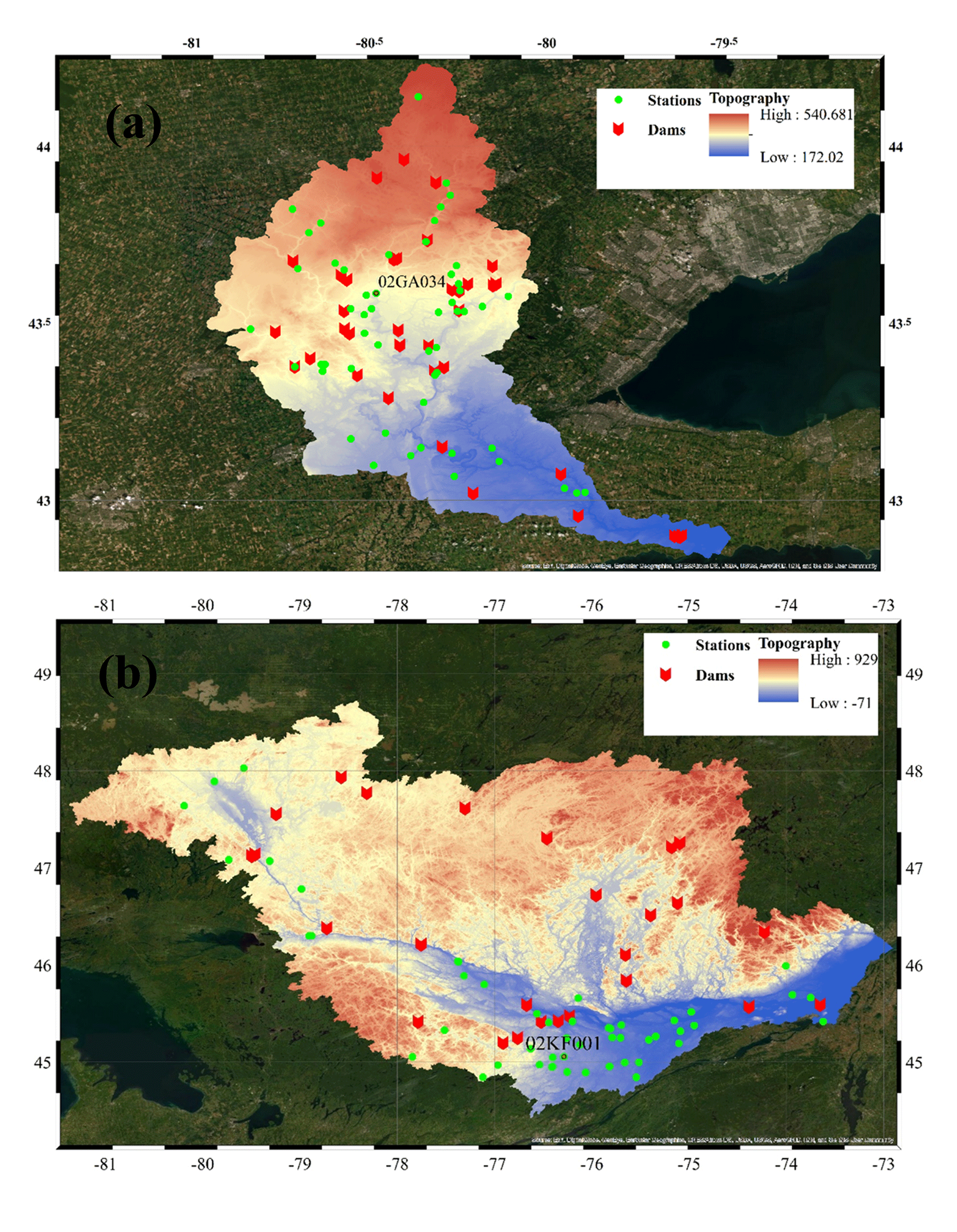
Figure 1 GIS input data – Grand River watershed (a) and Ottawa River watershed (b) topography. The maps are created in ArcGIS with the basemaps provided by © Esri. The stations that are used later in the Fig. 5 comparison are labeled in the plot.

Table 1 Values of Manning's n.

2.2 Modeling

2.2.1 Stage 1: GIS pre-processing

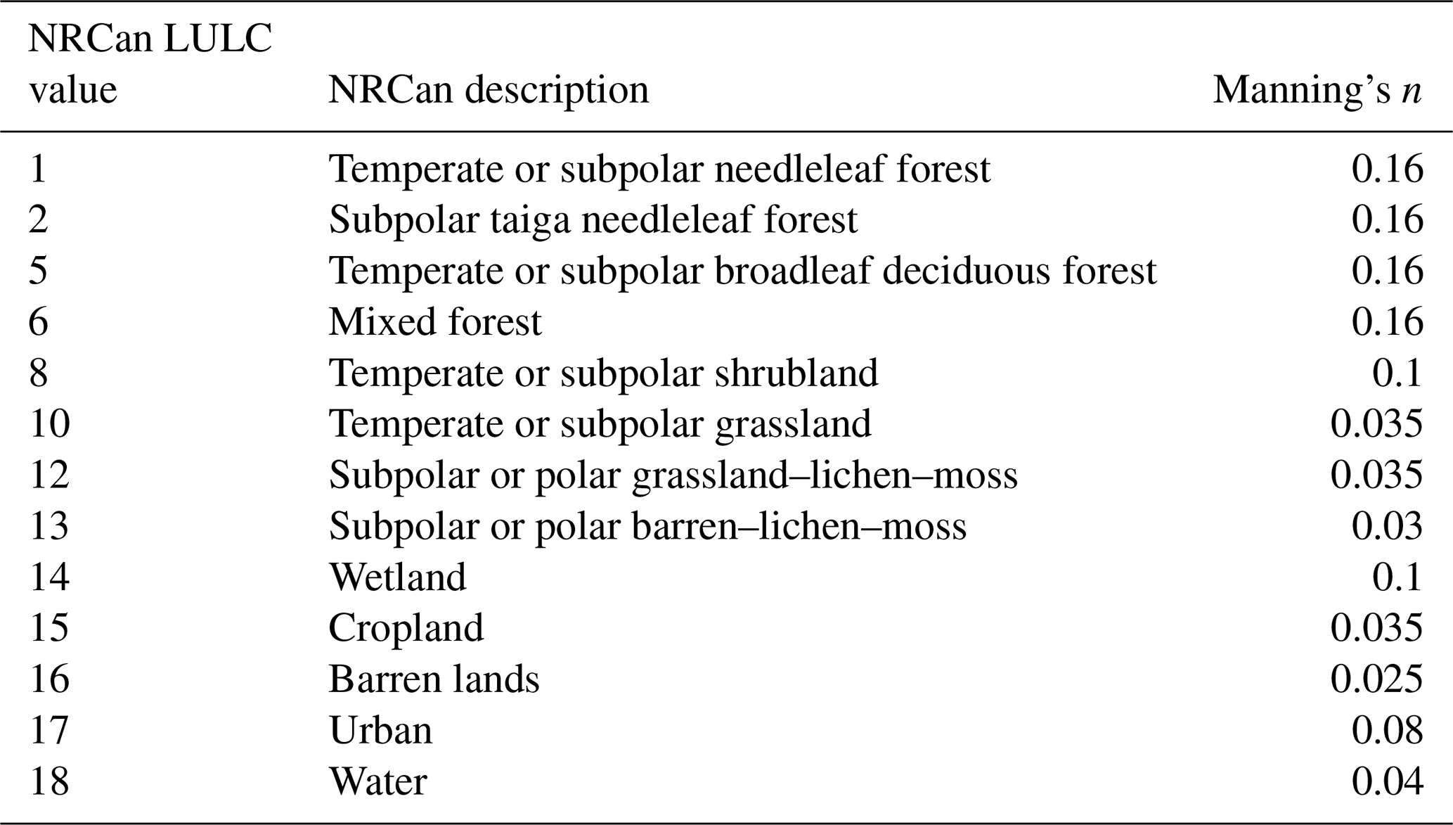
The following GIS input data were obtained from Natural Resources Canada for the Grand River and Ottawa River watersheds and cropped to their respective drainage areas of 6800 km² (Li et al., 2016) and 146 000 km² (Nix, 1987): digital elevation models (DEMs) (Canada Centre for Mapping and Earth Observation, 2015); river network vector shapefiles (Strategic Policy and Innovation Centre, 2019); and land use/land cover (LULC) (Canada Centre for Remote Sensing, 2019). Figure 1 shows the input DEM with elevation values given in meters, and the dams and gauging stations used in this study. The resolution of the DEM and LULC data is 30 m × 30 m. The vertical accuracy of the DEM is 0.34 m ± 6.22 m, i.e., 10 m at the 90 % confidence level (Beaulieu and Clavet, 2009). The vertical datum used is the Canadian Geodetic Vertical Datum of 2013 (CGVD2013). The stations used for station-level discharge comparison are labeled in Fig. 1. The uncertainty in the vertical dimension affects the slopes of individual pixels and the upslope contributing area and can potentially affect the quality of extracted hydrologic features (Lee, 1996; Lee et al., 1992; Liu, 1994; Ehlschlaeger and Shortridge, 1996). Hunter and Goodchild (1997), while investigating the effect of simulated changes in elevation at different levels of spatial autocorrelation on slope and aspect calculations, indicated the importance of a stochastic understanding of DEMs. The Monte Carlo method (Fisher, 1991) could potentially shed some light on this kind of uncertainty. However, in our case, it was beyond the focus of our study, and we considered the vertical uncertainty small enough to not affect our large-scale flood modeling simulations. The remaining GIS input data are shown in Fig. S1 in the Supplement. Very small networks, independent of the higher-order channels, were deleted from both regions. ArcGIS Desktop's raster calculator tool was used to burn the river network vector into the DEM to ensure the consistency of the river network between the DEM delineated and observed. TauDEM (Terrain Analysis Using Digital Elevation Models) (Tarboton, 2005), an open-source tool for hydrological terrain analysis, was then used to determine drainage directions and drainage accumulation (Tarboton and Ames, 2004) within the watersheds of interest. Each watershed's drainage network was then established in TauDEM by defining a minimum threshold of 2 km² on the contributory area of each pixel for the Grand River watershed and 10 km² for the Ottawa River watershed. Separately, a value of Manning's n was determined for each 30 × 30 m pixel of the study areas based on land use/land cover attributes (Brunner, 2016). To this end, the input LULC classes (Canada Centre for Remote Sensing, 2019) within the study watersheds were mapped to the nearest class of the similar land cover classes documented in Chow (1959, Tables 5–6) and Brunner (2016, Figs. 3–19), from which the respective values of Manning's n were used. Table 1 provides the utilized input LULC classes, their respective description provided by Natural Resources Canada (NRCan), and the employed n values. HAND (Rahmati et al., 2018; Garousi-Nejad et al., 2019) was also calculated in TauDEM with reference to the DEM and derived drainage network. Figure 2a provides a visual overview of this stage of the modeling component.

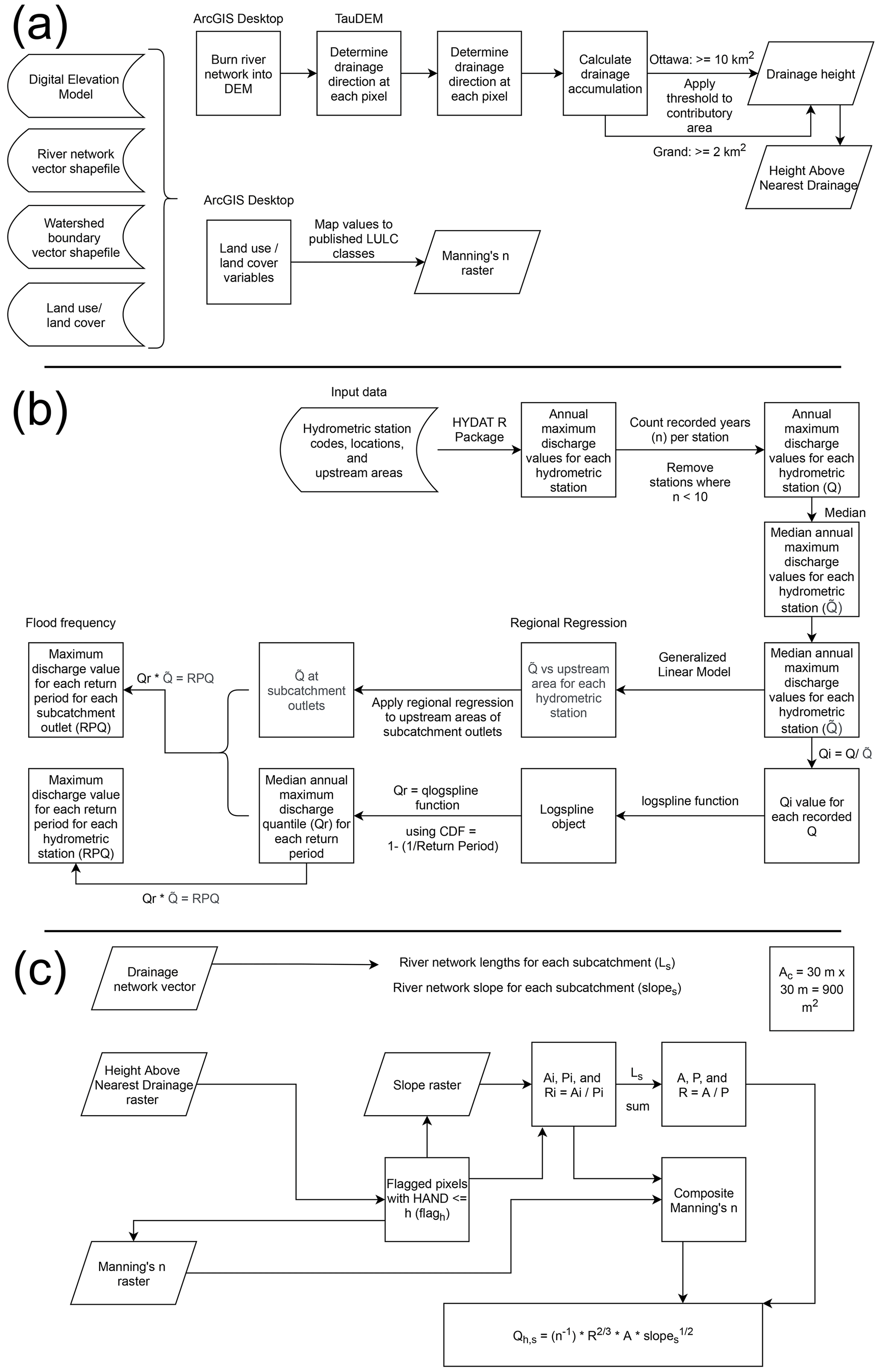
Figure 2 Flood model flow chart illustrating three subphases of overall modeling methodology: (a) GIS pre-processing; (b) flood frequency analysis and regional regression; and (c) HAND-based solution of Manning's equation.

2.2.2 Stage 2: regional regression and flood frequency analysis

Perhaps one of the most popular methods of flood frequency analysis is the index flood approach – a regional regression model based on annual maximum discharge data (Dalrymple, 1960; Hailegeorgis and Alfredsen, 2017). A variant of the index flood approach, which entails flood frequency analysis, has been employed to understand the characteristics of flood behavior at the global level (Smith et al., 2014). At regional scale, Burn (1997) has discussed the catchment procedure essential to undertake the flood frequency analysis. Faulkner et al. (2016) devised the procedure to estimate the design flood levels using the available station data. Regional hydrological frequency analysis at ungauged sites is also studied by few researchers (Desai and Ouarda, 2021).

The index flood approach was used to derive the discharge by return period at subcatchment outlets. The model includes two sections: (a) a relationship between index flood and contributory upstream area for each hydrometric station and each subcatchment outlet (regional regression); and (b) a flood frequency analysis to estimate the quantile values of the departures, with a departure defined as discharge at given station divided by the index flood of that same station). The index flood approach entails the following assumptions: (a) the flood quantiles at any hydrometric site can be segregated into two components – an index flood and regional growth curve (RGC); (b) the index flood at a given location relates to the (sub)catchment characteristics via a power-scaling equation, either in a simpler case which considers only upstream contributory area or in a more complex case which incorporates land use/land cover, soil, and climate information; and (c) within a homogeneous region the departure or ratio between the index flood and discharge at hydrometric sites yields a single regional growth curve which can relate the discharge and return period (Hailegeorgis and Alfredsen, 2017).

Per assumption (a) (the flood quantiles at any hydrometric site can be segregated into two components – an index flood and RGC), the index flood at each hydrometric station is required. To this end, annual maximum discharge values (m³ s⁻¹) were extracted within R (R Core Team, 2019) at hydrometric stations maintained by Environment Canada within the Grand River and Ottawa River watersheds (HYDAT) (Hutchinson, 2016). Only stations with a period of record >= 10 years of annual maximum discharge (England et al., 2018; Faulkner et al., 2016) were maintained (n=32 and n=54, respectively, for the Grand River watershed and the Ottawa River watershed). The minimum, median, and maximum periods of record for the Grand River watershed were 12, 50, and 86 years, respectively. Periods of record for the Ottawa River watershed ranged from a minimum of 10 years to a maximum of 58 years with a median of 36 years. A median annual maximum discharge value ($\stackrel{\mathrm{̃}}{Q}$) was then calculated for each hydrometric station. As discussed in Hailegeorgis and Alfredsen (2017), although the index flood is generally the sample mean of a set of annual maximum discharge values, index floods have also been evaluated based on the sample median (e.g., Wilson et al., 2011) at the suggestion of Robson and Reed (1999). Finally, the index flood values ($\stackrel{\mathrm{̃}}{Q}$) were used to normalize the observed annual maximum discharge values (Q) at their respective station, resulting in a set of values designated as Q_i, such that $Q_i=Q/\stackrel{\mathrm{̃}}{Q}$.

With respect to regional regression and assumption (b) of the index flood method, a generalized linear model was applied to relate log₁₀ transformed $\stackrel{\mathrm{̃}}{Q}$ values to log₁₀ transformed upstream area values at each hydrometric station. The generalized linear model assumed an ordinary least squares error distribution. The results of the generalized linear model for each watershed allowed for the calculation of previously unknown $\stackrel{\mathrm{̃}}{Q}$ values for each subcatchment outlet. In a more complex model (Fouad et al., 2016), other catchment characteristics such as land use/land cover, geology, etc. could be used. However, in the case of the proposed model, the correlations between the calculated and observed index floods, on the sole basis of discharge records and a linear model relating upstream area, were high as discussed in the Results section. Thus, the simpler method was used to estimate index floods and to relate index flood to contributory area at hydrometric stations and subcatchment outlets. Thus, the regional regression model derived a relationship between index flood ($\stackrel{\mathrm{̃}}{Q}$) and upstream contributory area for each hydrometric station s or subcatchment outlet. The relationship between index flood at station i or at a subcatchment outlet ($\stackrel{\mathrm{̃}}{Q^{\text{s}}})$ (median of annual maximum discharge) and upstream contributory area (A_s) is given by

$$\begin{array}{}\text{(1)}& {\stackrel{\mathrm{̃}}{Q}}^{\text{s}}=a{A}_s^c,\end{array}$$

where a is the index flood discharge response at a unit catchment outlet (or at a hydrometric station) and c is the scaling constant. We took the logarithm of Eq. (1) on both sides – a procedure noted in Hailegeorgis and Alfredsen (2017) as used in Eaton et al. (2002) – yielding a linear relationship which was solved using the ordinary least squares approach (Haddad et al., 2011).

With respect to assumption (c) of the index flood method, which assumes that a regional growth curve can be applied to a homogenous area as outlined above, we attempted to fit a distribution to the ratio of the annual maximum discharge values at each station to the corresponding index flood. Hailegeorgis and Alfredsen (2017) discussed a regionalization procedure which ensures the homogeneity of the station-level data over any region. However, due to the limited availability of the discharge data, we avoided such subsampling and carried out the index flood method at the entire watershed scale (Faulkner et al., 2016). This, however, has impacted the upper quantiles of the flood estimation when comparing to the station-level data (Sect. 3.1). A fundamental step of the analysis process is the selection of a suitable probability distribution model, a common tool in hydrologic modeling studies. The model should account for changes to the flow's extreme value characteristics in response to such factors as urbanization, agriculture, resource extraction, or the operation of dams and weirs. Sometimes, natural hydrologic peaks, such as the spring freshet, are exacerbated by antecedent conditions such as large snowpacks and frozen soils, resulting in substantial flood events. While solutions to this problem have been proposed in the literature, artificial abstraction fundamentally changes the extreme value characteristics of the flow, thereby hindering the usability of most distributional forms (Kamal et al., 2017).

Many researchers have tried to address this problem by putting explicit assumptions on types of non-stationarity affecting the river discharge and are able to devise a closed mathematical formulation which enables the parametric distributions to handle such non-stationarity. However, such methods typically entail knowledge of the specific design return periods of individual flood prevention structures (Salas and Obeysekera, 2014), many of which are absent in our case. To circumvent this problem, we used a non-parametric approach for the RGC, which requires no fundamental sample characteristics. Thus, modified flood records and limited information notwithstanding, flood frequency estimation is possible using the index flood approach. Per assumption (c) of the index flood method, a log-spline non-parametric approach was taken to model a RGC (Stone et al., 1997) for each study watershed. Specifically, the index flood values ($\stackrel{\mathrm{̃}}{Q}$) were used to normalize the observed annual maximum discharge values (Q) at their respective station ($Q_i=Q/\stackrel{\mathrm{̃}}{Q}$). The Q_i values (n= 1487 and n= 1248 for the Ottawa River watershed and the Grand River watershed, respectively) were then fitted to a log-spline distribution for their respective watershed. The discharge quantiles (Q_r) were extracted for the following return periods (T, years): 1.25, 1.5, 2.0, 2.33, 5, 10, 25, 50, 100, 200, and 500. The return periods were first converted to a cumulative distribution function.

Finally, flood quantile estimations were calculated for each return period as shown below:

$$\begin{array}{}\text{(2)}& Q_T^i=\stackrel{\mathrm{̃}}{Q^i}{q}_T,\end{array}$$

such that T is a specified return period in years; $Q_T^i$ is a quantile estimate of discharge for the specified return period T (years) at a specified station i (or a subcatchment outlet); $\stackrel{\mathrm{̃}}{Q^i}$ is the “index flood” at the same station i (or at the same subcatchment outlet); $i=\mathrm{1},\mathrm{2},\mathrm{\dots }N$, where N=32 for the Grand River watershed or N=54 for the Ottawa River watershed; and q_T is the regional growth curve as described above. Figure 2b provides a visual accounting of the regional regression and flood frequency analysis methodology described in this section.

Some of the limitations of this framework include the long-term flow records and homogenous stations required for the creation of regional regression models. A dearth of long-term data affects flood magnitude computations specifically for the upper quantiles (5T rule, Sect. 3.1).

2.2.3 Stage 3: catchment-integrated Manning's equation

Manning's formula (Song et al., 2017) is widely used to calculate the velocity and subsequently the discharge of any cross-section of an open channel. Manning's equation is given in SI units by

$$\begin{array}{}\text{(3)}& Q={\displaystyle \frac{\mathrm{1}}{n}}{R}_{\text{h}}^{\frac{\mathrm{2}}{\mathrm{3}}}A{S}^{\frac{\mathrm{1}}{\mathrm{2}}},\end{array}$$

such that Q is discharge in cubic meters per second, A represents the cross-sectional area, n is a roughness coefficient, R_h is the hydraulic radius, and S represents slope (fall over run) along the flow path. Despite its widespread use, robustness, and relative ease of use, Manning's equation has an inherent problem which comes from the uncertain orientation of cross-sections. To mitigate this problem, we integrated Manning's equation along the drainage lines within the catchment, accounting for the slope of each grid cell to yield bed area and derived the stage–discharge relationship. This strategy uses hydrological terrain analysis, discussed previously in Sect. 2.2.1, to determine the HAND of each pixel (Rodda, 2005; Rennó et al., 2008). The HAND method determines the height of every grid cell to the closest stream cell it drains to. In other words, each grid cell's HAND estimation is the water height at which that cell is immersed. The inundation extent of a given water level can be controlled by choosing all the cells with a HAND less than or equal to the given level. The water depth at every cell can then be calculated as the water level minus the HAND value of the corresponding cell. The relevance of HAND to the field of flood modeling has been demonstrated in the literature (Rodda, 2005, Nobre et al., 2016). Its documented use notwithstanding, HAND's potential applications to the depiction of stream geometry information and to the investigation of stage–discharge connections have not been well investigated. Hydraulic methods of discharge calculation typically entail hydraulic parameters derived from the known geometry of a channel. The knowledge of a channel's cross-sectional design is a requirement for many one-dimensional flood routing models, for instance, the one-dimensional St. Venant equation (Brunner, 2016). Even though the use of DEM-interpolated bathymetry, as used by our method, induces error in the modeling of flood inundation, it is a necessity in the absence of bathymetry data. We assumed the underestimation of channel conveyance due to the use of interpolated DEM bathymetry to be negligible. There are several instances in literature (Sanders, 2007) where the DEM-interpolated bathymetry has been tested in place of actual bathymetry for hydrodynamic flood modeling. Furthermore, the requirement of the cross-section being perpendicular to the flow direction makes it an implicit problem and also dependent on the choice of cross-section position as well as the distance at which the points are taken on the cross-section. In the current practice of hand designing, it makes it subjective and draws substantial uncertainty in the inundation simulation. Alternatively, HAND-based models do not explicitly solve Manning's equation at individual cross-sections but rather solve for a catchment-averaged version of it by considering a river as a summation of infinite cross-sections. As such, the inherent uncertainty is avoided. However, the simplistic HAND-based model struggles to simulate proper inundation extent in the case of complex conditions such as meandering main channels and confluences (Afshari et al., 2018). This model does not capture the dynamic flow characteristics such as backwater effects created by flood mitigation structures. Furthermore, the large flood depth and low flow velocity in the natural rivers makes the river subcritical on many occasions, specifically for large floodplains where the water slows down significantly. This causes the backwater effect very far upstream of the flooding locations which is not simulated in HAND-based methods. Therefore, users have to be cautious in such cases.

The conceptual framework for implementing HAND to estimate the channel hydraulic properties and rating curve is as follows: for any reach at water level h, all the cells with a HAND value <h compose the inundated zone F(h), which is a subarea of the reach catchment. The water depth at any cell in the inundated zone F(h) is the difference between the reach-average water level h and the HAND of that cell, HAND_c, which can be represented as depth equal to HAND_c−h. Since a uniform reach-average water level h is applied to check the inundation of any cell within the catchment, the inundated zone F(h) refers to that reach level. The water surface area of any inundated cell is equal to the area of the cell A_c. This case study uses 30 m × 30 m grid cells; thus, in this case, A_c=900 m². The channel bed area for each inundated cell is given by

$$\begin{array}{}\text{(4)}& A_s=A_{\text{c}}\sqrt{(\mathrm{1}+{\text{slope}}^{\mathrm{2}})},\end{array}$$

where “slope” is the surface slope of the inundated pixel expressed as rise over run or inverse tangent of the slope angle. This equation approximates the surface area of the grid cell as the area of the planar surface with surface slope, which intersects with the horizontal projected area of the grid cell. The flood volume of each inundated pixel at a water depth of h can be calculated as $V_{\text{c}}\left(h\right)=A_{\text{c}}(h-{\text{HAND}}_{\text{c}})$. If the reach length L is known, the reach-averaged cross-section area for each pixel is given by $A_i=V_{\text{c}}/L$. Similarly, the reach-averaged cross-section wetted perimeter for each inundated pixel $P_i\left(h\right)=A_s/L$. Therefore, the hydraulic radius for each inundated pixel (i) is given by $R_i=A_i/P_i$. Therefore, we can estimate the reach-averaged cross-section area $A={\sum }_i{A}_i$, perimeter $P={\sum }_i{P}_i$, and hydraulic radius $R=A/P$ for the entire flooded area. We compared the composite Manning's n (Chow, 1959; Flintham and Carling, 1992; Pillai, 1962; Tullis, 2012) from seven different methods: the Colebatch method; the Cox method; the Horton method; the Krishnamurthy method; the Lotter method; the Pavlovskii method; and the Yen method (McAtee, 2012). More details about these methods are in Sect. S2 of this paper.

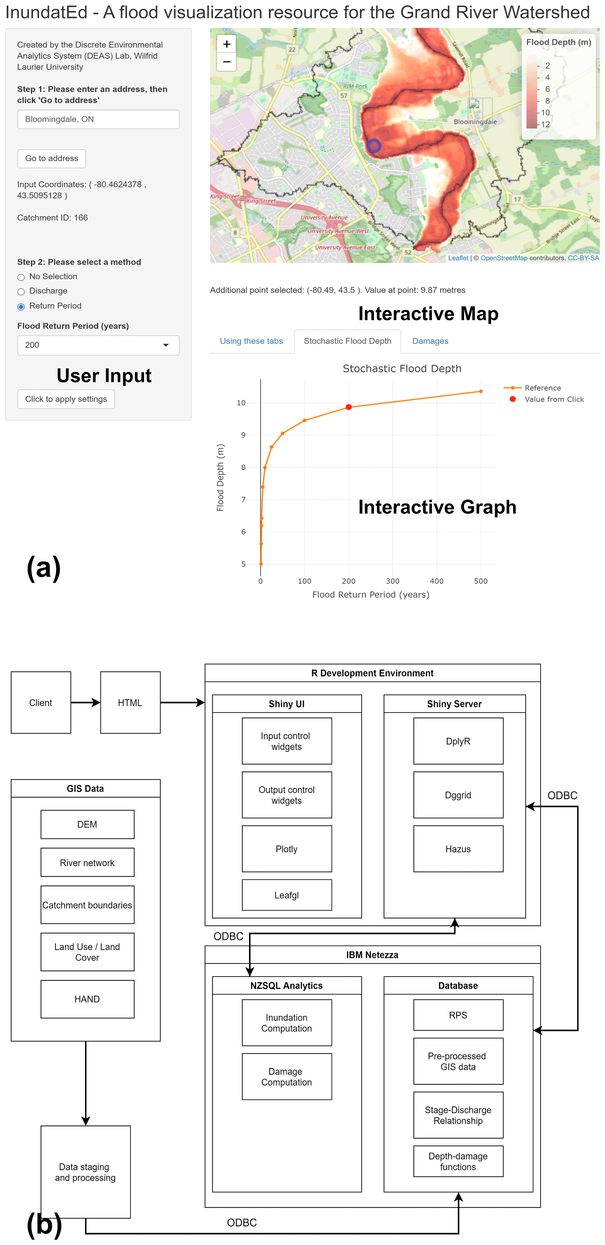
Figure 3 InundatEd user interface (a) and system diagram (b). The basemap is created in Leaflet using © OpenStreetMap contributors 2020. Distributed under a Creative Commons BY-SA License.

Thus, the discharge Q(h) corresponding to inundation height can be computed by the Manning equation and given by

$$\begin{array}{}\text{(5)}& Q\left(h\right)={\displaystyle \frac{\mathrm{1}}{n}}{R}^{\frac{\mathrm{2}}{\mathrm{3}}}A{S}^{\frac{\mathrm{1}}{\mathrm{2}}},\end{array}$$

where S is the slope of the river and n is the composite Manning's roughness coefficient. Figure 2c displays the sequence of methods outlined for the catchment-integrated Manning's equation method.

2.2.4 Stage 4: upscaling and data conversion

The proposed InundatEd inundation model simulates the flood-depth distributions for each catchment independently. This makes this model suitable to be ported to a DGGS-based data model and processing system. Following the GIS pre-processing, done in TauDEM as discussed in Sect. 2.2.1, the required data were converted to a DGGS representation, as outlined in Robertson et al. (2020). Figure S2 shows raster input data (panel a), polygon (vector) input data (panel b), and network (directional polyline vector) input data (panel c). For raster data (panel a), the bounding box is used to extract a set of DGGS cells, and then for each DGGS cell's centroid the raster value is extracted. To convert polygon data to a DGGS data model, we sample from its interior and its boundary separately using uniform sampling. Then each sample point is converted into DGGS cells based on its coordinates and stored into IDEAS data model by aggregating both sets of DGGS cells (Fig. S2b). The same process for the border extraction is applied to the polylines and networks; however, with network data, the order of the cells is also stored as a flag to use in directional analysis (Fig. S2c). Following conversion, the data were ported to a 40-node IBM Netezza database for subsequent calculations. General, systematic limitations of the InundatEd IDEAS-based inundation model are discussed in Sect. 3.1.

2.3 Web-GIS interface

The R/Shiny platform and the R Studio development environment were used to design the user interface and server components of an online web application, allowing users to query and interact with the inundation model. Features of R specific to InundatEd's modeling workflow were its support of the Hazus damage functions and its support for DGGS spatial data. Shown in Fig. 3a, the InundatEd user interface offers widgets for the following user inputs: address (text), discharge (slider), and return period (drop down), as well as tabs for viewing interactive graphs. The InundatEd user interface also features an interactive map which leverages the Leafgl R package (Appelhans and Fay, 2019) for seamless integration with the DGGS data model. Users may click on the map to obtain point-specific depth information.

2.4 InundatEd flood information system – system structure summary

Figure 3b displays the overall system structure and linkages for the InundatEd flood information system. GIS input data, as discussed in Sect. 2.2, were staged, pre-processed, and ported to the database. Data querying was used to compute “in-database” inundation (flood depth) and related damages (methods outlined in Sect. 2.1) in response to user interface inputs to the R/Shiny UI.

Table 2 Study watershed characteristics.

2.5 Flood data comparison and model testing

2.5.1 Study areas

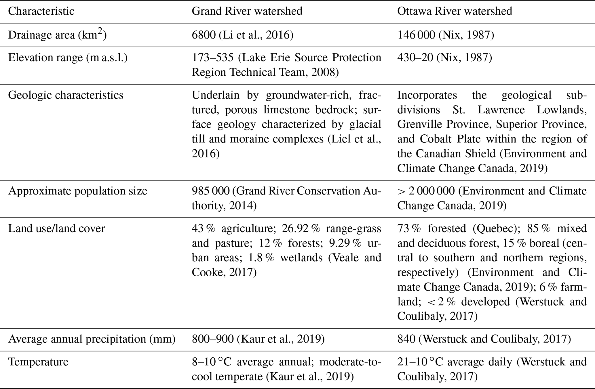
As preliminary testing domains, we created flood inundation models for the Grand River basin and Ottawa River basin, respectively, both located in Ontario, Canada. Each basin has experienced historical flooding and has implemented varying measures of flood control. Table 2 shows different salient characteristics of these catchments. For the purposes of graphing and discussion of station-specific period of record (number of years with a recorded annual maximum discharge) on theoretical vs. estimated flood quantiles, two stations from each study watershed were selected: one each for high period of record and low period of record. For the Grand River watershed, stations 02GA003 and 02GA047 were selected for high and low periods of record, respectively. For the Ottawa River watershed, stations 02KF006 and 02JE028 were selected, respectively. “Theoretical quantiles” are here defined as the quantiles generated by our model based on the log-spline fit, which incorporates annual maximum discharge values from multiple stations across each study watershed (Sect. 2.2.2 and Fig. 3). In contrast, “estimated quantiles” are here defined as the flood quantiles calculated simply by extracting the quantiles for the desired return periods from the raw annual maximum discharge values observed at the hydrometric station of interest.

2.5.2 Ottawa River watershed

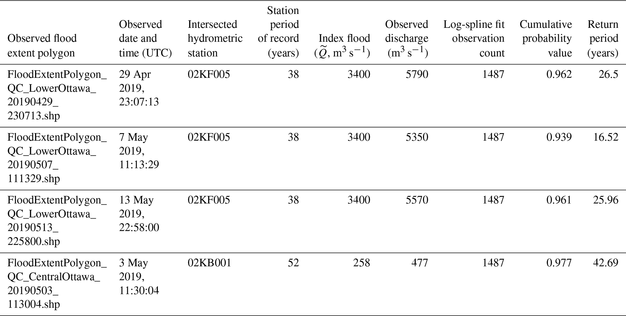
Four flood extent polygons (FEPs) provided by Natural Resources Canada (Natural Resources Canada, 2018, 2020) from the May–June 2019 flood season were used as “observed” floods to test the model outputs for the Ottawa River watershed. Each FEP represented a previously digitized floodwater extent at a specified date/time.

A second criterion for selection was that the hydrometric station(s) intersected by the FEP provided discharge data for the FEP's respective date/time. Two hydrometric stations which met both criteria were selected: 02KF005 and 02KB001. The following procedure was followed for each FEP using the corresponding hydrometric station (02KF005 or 02KB001), the station-level index flood ($\stackrel{\mathrm{̃}}{Q}$, previously calculated in Sect. 2.2.2), and the observed discharge (Q_obs). In both cases, the log-spline fit for the Ottawa River watershed, previously generated in Sect. 2.2.2, was also used.

The observed discharge (Q_obs) was divided by the corresponding hydrometric station's index flood ($\stackrel{\mathrm{̃}}{Q}$) ($Q_i=Q_{\text{obs}}/\stackrel{\mathrm{̃}}{Q}$). The cumulative probability of Q_i was then converted to a return period.

To generate each simulated flood for comparison to its observed counterpart, the methodology outlined in Sect. 2.2.2 and 2.2.3 was repeated with the four new return periods appended to the original list of return periods in Sect. 2.2.2. Table 3 lists each FEP, the corresponding intersected hydrometric station, the period of record used for each station to calculate $\stackrel{\mathrm{̃}}{Q}$, the observed discharge, the resultant cumulative probability value, and the final return period used to generate each simulated flood.

Table 3 Simulated Flood Generation – Ottawa River Watershed.

2.6 Grand River watershed

Regulatory floodplain extent data (the greater of a return period (RP) of 100 or discharge from Hurricane Hazel, “observed” flood extent) were obtained from the Grand River Conservation Authority (GRCA) (Grand River Conservation Authority, 2019). However, analysis revealed that, at most hydrometric stations in the Grand River watershed, the 100-year return period yielded higher discharge values relative to the Hurricane Hazel storm. Thus, the 100-year return period could be used. The estimated flood extent for RP of 100 was generated per Sect. 2.2.1–2.2.3. Table S1 provides a discharge comparison between the 100-year return period and the regulatory storm.

2.7 Flood extent comparisons

For both the Grand River watershed and the Ottawa River watershed, only those subcatchments in close proximity to the observed flood extent polygons were retained for visualization purposes. To this end, a criterion was applied to subcatchments in the Grand River watershed requiring an intersection with the observed flood polygon of >= 20 % of the subcatchment's area. For the Ottawa River watershed, due to the use of station-specific observed discharge, an additional criterion was applied: that a given subcatchment intersects with a network line with contributory upstream area >= 80 % and contributory upstream area $<=$ 120 % of the observed upstream area of the hydrometric station (02KF005 or 02KB001). Table S2 provides by-subcatchment areas of the observed flood extent polygons whose subcatchments were eliminated based on the 20 % intersection threshold. Per Table S2, one excluded subcatchment (10505) had an intersection value >= 20 %, attributable in part to the presence of a tributary along which it was not expected that the return period would be properly scaled but which intersected the subcatchment. Additionally, due to the pluvial nature of the flooding in that subcatchment, it was once again expected that the return period as a function of the river discharge would not be properly scaled without the presence of a hydrometric station to provide discharge information.

Binary classification metrics have been used to compare between observed and simulated floods in cases where the focus is on extent, not depth (e.g., Papaioannou et al., 2016; Wing et al., 2017; Chicco and Jurman, 2020). A binary classification (or 2×2 contingency) method was used to compare the simulated flood extent rasters to the extents of their observed counterparts, whereby a confusion matrix was generated for each subcatchment. Multiple accuracy measures were calculated from the contingency tables to support the evaluation of the flood model, including true positive rate (TPR), true negative rate (TNR), accuracy, Matthews correlation coefficient (MCC) (Chicco and Jurman, 2020; Esfandiari et al., 2020; Rahmati et al., 2020), and the critical success index (CSI) (e.g., Papaioannou et al., 2016; Stephens and Bates, 2015). Both the CSI and the MCC have been used in the context of flood model validation. The CSI is defined as

$$\begin{array}{}\text{(6)}& \text{CSI}={\displaystyle \frac{\text{TP}}{\text{TP}+\text{FN}+\text{FP}}}.\end{array}$$

The MCC is defined as

$$\begin{array}{}\text{(7)}& \text{MCC}={\displaystyle \frac{\text{TP}\times \text{TN}-\text{FP}\times \text{FN}}{\sqrt{\left(\text{TP}+\text{FP}\right)\left(\text{TP}+\text{FN}\right)(\text{TN}+\text{FP})(\text{TN}+\text{FN})}}},\end{array}$$

such that TP is a true positive, TN is a true negative, FP is a false positive, and FN is a false negative.

Figure 4 Flood frequency and regional regression plots.

3 Results and discussion

3.1 Model processes and DGGS

Intermediate model outputs for the Grand River and Ottawa River watersheds – HAND, delineated river networks, and Manning's n – are displayed in Fig. S3. Figure 4 visualizes results for the Grand River watershed and for the Ottawa River watershed for the following method components: calculation of hydrometric station upstream (contributory) area; index flood regression as represented by the correlation of logged index discharge and logged upstream area; and flood frequency as represented by discharge against a Gumbel transformed return period (years), for the stations, respectively, representative of high and low observations. Figure 4a and b plot the log of calculated upstream area against the log of observed upstream area, yielding respective Pearson correlation coefficients of 0.99 and 0.63 for the Grand River and Ottawa River watersheds. The relatively weak correlation of the Ottawa River watershed arose primarily from the limited resolution (number of decimal places in lat–long) of the station location information; incorrect reporting of station locations and/or their drainage area (Environment Canada reported the drainage area as 0 for multiple stations); and sometimes wrongly snapping stations to the tributaries rather than to the main river, particularly in cases involving a wide river channel or braided river.

Figure 5 Theoretical vs. estimated flood quantiles.

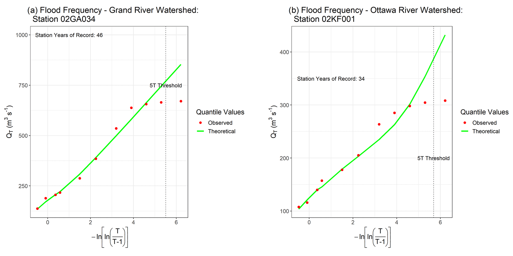
However, this does not affect the model itself, as we have used the station-specific drainage areas reported by Environment Canada to create the regional regression model. With respect to regional regression, Fig. 4c visualizes the relationship between predicted index flood discharge and contributory upstream area, at individual hydrometric stations, for the Grand River and Ottawa River watersheds (R= 0.83 and 0.95, respectively). The regional growth curves for both the Grand River watershed and the Ottawa River watershed are shown in Fig. 4d. To compare the proposed approach of using log-spline distribution against a traditional parametric distribution we fitted a generalized extreme value (GEV) distribution to the RGC (Fig. S4). With respect to the log-spline RGCs, Akaike information criterion (AIC) values of 1861.69 and 867.69 and (−2) (log likelihood) values of 1826.04 and 809.26 were reported for the Grand River watershed and Ottawa River watershed, respectively. The log-spline (−2) (log likelihood) values were lower than their GEV counterparts (1837.56 and 880.12) for both watersheds. For the Ottawa River watershed, the log-spline AIC value, 867.69, was also lower than that of its GEV counterpart (886.12). Furthermore, the use of the log-spline distribution allows for a consistent method which can be applied readily across any watershed without careful calibration of the distribution function. Thus, the log-spline distribution was used for the regional growth curves. The lower values of the normalized discharge shown in Fig. 4d for higher return periods (2–3) for the Ottawa River watershed suggest relatively more structural alterations within the watershed, for instance, flood control and dams, than the Grand River watershed (Ottawa Riverkeeper, 2020). The Grand River watershed yielded relatively higher values of normalized discharge (> 3) at higher return periods in Fig. 4d. Figure 5 shows the comparison of estimated flood quantiles against theoretical flood quantiles at an individual station from each study watershed. The stations – 02GA034 of the Grand River watershed and 02KF001 of the Ottawa River watershed (Fig. 1) – were selected due to their long “discharge counts”, referring to the number of years for which an annual maximum discharge was recorded at each station. Specifically, station 02GA034 (Fig. 5a) yielded a discharge count of 101 and station 02KF001 (Fig. 5b) yielded a discharge count of 84. Return periods (T, years) have been converted in terms of the Gumbel reduced variable as follows:

$$\begin{array}{}\text{(8)}& \text{Gumbel}=-\ln \left[\ln \left({\displaystyle \frac{T}{T-\mathrm{1}}}\right)\right].\end{array}$$

The dotted lines in Fig. 5a and b represent the 5T threshold – the return period limit beyond which flood simulations cannot be reasonably estimated. The 5T threshold requires that, for the reasonable estimation of a quantile for a desired return period T, there be at least 5T years of data (Hailegeorgis and Alfredsen, 2017; Jacob et al., 1999). As expected, the theoretical and estimated return periods are comparable for low return periods. However, and as shown in Fig. 5, the theoretical and estimated quantiles deviate at lower RP values than the 5T threshold for both stations. This disagreement between the theoretical and estimated quantiles recalls the assumption of homogeneity for each watershed (Burn, 1997) – estimations of higher return periods, considering the 5T rule, would require more observations. However, further subsampling the stations into regional homogeneous groups would have reduced the data quantity substantially for each group.

3.2 Web-GIS interface

A pre-alpha version of the InundatEd app is available at https://spatial.wlu.ca/inundated/ (last access: 20 May 2021). Source code for the most recent version of InundatEd will be publicly available on GitHub (Spatial Lab, 2020). The use of R/Shiny to develop InundatEd and its provision on GitHub encourages transparency, ongoing development, and response to user feedback and preferences.

3.3 Model testing

Of the binary comparison results for the seven composite Manning's n methods listed in Sect. 2.2.3, the Krishnamurthy method yielded the highest median CSI values (Table S3 for the Grand River watershed and Table S4 for the Ottawa River watershed). As such, it was selected for further visualization and discussion.

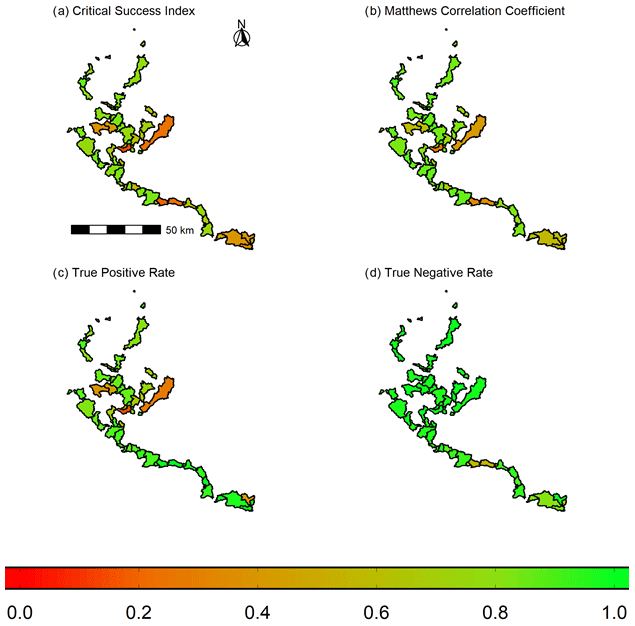
Figure 6 Binary classification results – Grand River watershed.

The following return periods (in years) were observed for FEPs intersecting hydrometric station 02KF005 in the Ottawa River watershed: 26.5, 16.52, and 25.96. Additionally, a return period of 42.69 years was observed for a FEP intersecting hydrometric station 02KB001 in the Ottawa River watershed. The 100-year return period was tested for the Grand River watershed. Binary classification results for the Grand River watershed are shown in Fig. 6 for four comparison metrics: critical success index, Matthews correlation coefficient, true positive rate, and true negative rate. Figure 7 presents critical success index and Matthews correlation coefficient results for the four Ottawa River watershed cases, with true positive and true negative results presented in Fig. S5. Table 4 lists the number of subcatchments evaluated, the median CSI, and the median MCC for each of the five test return periods. The median values of additional metrics are provided in Table S5.

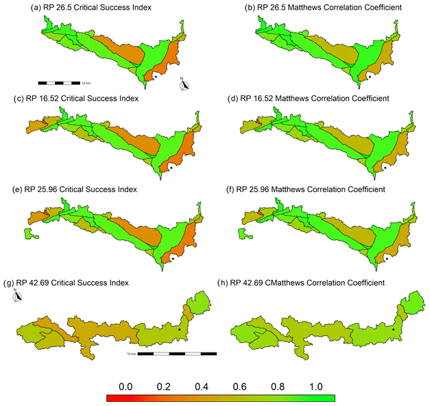
Figure 7 Binary classification results – Ottawa River watershed.

Table 4 Binary comparison results.

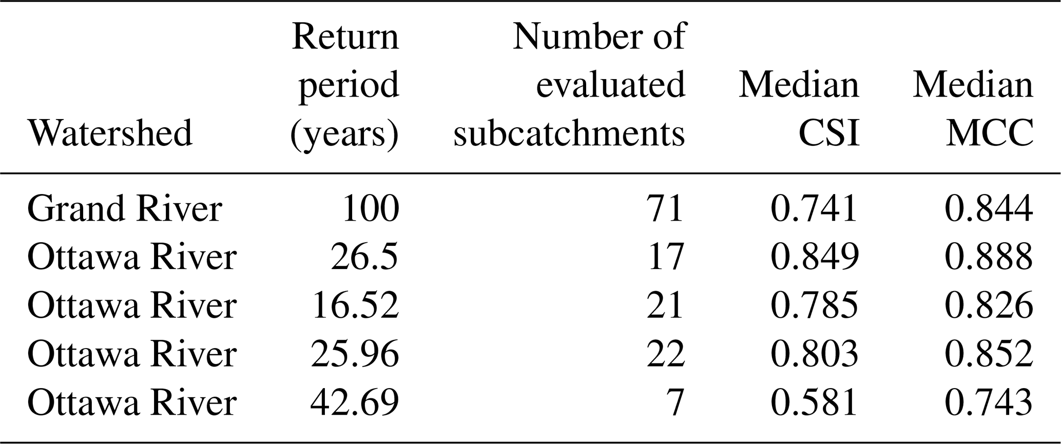
The median CSI values ranged from 0.581 to 0.849 (Table 4), with both of those values coming from the Ottawa River watershed (return periods 42.69 and 26.5, respectively). The median MCC values ranged from 0.743 (Ottawa RP of 42.69) to 0.888 (Ottawa RP of 26.5). The median CSI and MCC values for the Grand River watershed were 0.741 and 0.844, respectively. The results reported herein are comparable to, and in some cases exceed, previously published binary classification results. For instance, with respect to the MCC, an urban flood model produced by Rahmati et al. (2020) provided an MCC value of 0.76 when compared to historical flood risk areas. Esfandiari et al. (2020) compared two flood simulations: a HAND-based flood model and a model which combined HAND and machine learning to observe flood extents, resulting in a range of MCC values from ∼ 0.77 to ∼ 0.85. Bates et al. (2021) achieved CSI values of 0.69 and 0.82 for a 100-year return period flood model of the conterminous United States at a 30 m resolution. It must be noted that direct comparisons between the works listed here and this study must be viewed with caution, due to differences in methodologies, assumptions, data sources, data availability, and return periods between the studies. Furthermore, the extent comparison scores are not necessarily objective measures of performance of the simulation model. They can vary depending on the severity of the flood, catchment characteristics, and quality of the benchmark data (Mason et al., 2009; Stephens et al., 2014; Wing et al., 2021).

Figure 8 Simulated flood and insets – Grand River watershed 100-year return period.

Additionally, the median F₁ score (Chicco and Jurman, 2020) for the Grand River watershed was 0.85. The median F₁ scores for Ottawa River watershed return periods 26.5, 16.52, 25.96, and 42.69 were 0.96, 0.95, 0.95, and 0.94, respectively. Such results are approximately in line with Pinos and Timbe (2019), who achieved F₁ values from 0.625 to 0.941 for 50-year RP floods using a variety of 2-D dynamic models. Afshari (2018) achieved F₁ values from 0.48 to 0.64 for the 10-year, 100-year, and 500-year return periods when comparing a HAND-based simulation against a Hydrologic Engineering Center's River Analysis System (HEC-RAS) 2-D control. Lim and Brandt (2019) determined that low-resolution DEMs are capable of yielding relatively high comparison metrics (e.g., F₁ values approximately >= 0.80) in situations where Manning's n varies widely over space. The connection between high values of Manning's n and flood overestimation (false discovery) was also discussed. The Grand River watershed yielded a median false discovery rate (FDR) of 0.117, and the four Ottawa River watershed cases yielded respective median FDRs of 0.019, 0.01, 0.006, and 0.44 for the evaluated subcatchments. The moderately high FDR value of 0.44 for the 42.69-year return period and the observed overestimation of flood extent (discussed below) may be a result of high local Manning's n values. In addition, the influences of flat terrain (Lim and Brandt, 2019) and anabranch must be considered as it can disrupt the assumption of a single drainage direction for each pixel during subcatchment delineation. Additional factors potentially influencing the overestimation are the problems inherent to HAND-based modeling, as discussed in Sect. 2.2.3. The topography of the area of the Ottawa River watershed wherein the extent comparisons were made is relatively flat with multiple anabranches and thus can lead to chaotic network delineation. Although attempts were made in this model to counter this impact and avoid slope values of 0 (the burning of the polyline network into the DEM; Sect. 2.2.1 and Fig. 2a), the use of the Manning equation was still compromised in certain areas and likely had a negative impact on the resultant flood simulations.

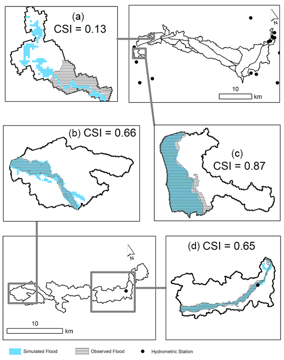
Figure 9 Observed and simulated flood extents – Ottawa River watershed.

As noted in Lim and Brandt (2019), the reliability of the observed flood extent polygons also merits comment. In this case study, the observed FEPs for the Ottawa River watershed were originally digitized from remotely sensed data and thus carry forward the errors and uncertainties from prior processing. The Grand River watershed's 100-year return period extent was also generated outside of this study and potentially carries multiple sources of error and uncertainty. However, evaluation of the exact extent to which errors present in the observed flood extent polygons could have impacted the binary classification results was not an objective of this study.

Figure 8 visualizes the 100-year return period simulated flood for the Grand River watershed. Inset maps are provided which highlight one subcatchment with a high CSI (Fig. 8a, CSI = 0.77) and two subcatchments with low CSIs (Fig. 8b, CSIs of 0.17 and 0.22). The simulated flood shown in Fig. 8a compares very well to the extent of its observed counterpart, consistent with the relatively high CSI value. Notably, three hydrometric stations are located within the Fig. 8a subcatchment: 02GA014, 02GA027, and 02GA016. Per the methods in Sect. 2.2.2, station 02GA014 yielded a period of record of 54, 02GA027 yielded an insufficient (< 10) period of record, and station 02GA016 yielded a period of record of 58. The presence of the two hydrometric stations with considerable periods of record likely strengthened the regional regression of the area and contributed to the success of the simulated flood shown in Fig. 8a. In contrast, within the low-CSI (0.17 and 0.22) subcatchments shown in Fig. 8b, the simulation considerably overestimated the extent of the 100-year return period flood. The overestimation of the flood extents observed in Fig. 8b can likely be attributed, at least in part, to the following: (a) multiple upstream and downstream dams (Grand River Conservation Authority, 2000) and (b) the channel meanders – as discussed previously, the simple HAND-based model employed here is not robust against channel complexities nor flow control structures such as dams. It must be recalled here that the modular nature of the InundatEd model allows for the “swapping” of various flood modeling methods and thus could easily accommodate, for instance, shallow water equations. It is also possible to include such operations in future versions of the model by either modifying the DEM values to reflect flood control structures or by offsetting the discharge of the catchment based on structure storage.

With respect to the Ottawa River watershed, Fig. 9 highlights subcatchments whose comparison between observed and simulated flood extents yielded low (Fig. 9a, CSI = 0.13), moderate (Fig. 9b, CSI = 0.66, and Fig. 9d, CSI = 0.65) and high (Fig. 9c, CSI = 0.87) CSI values.

Figure 9a shows the simulated and observed flood extents for return period 25.69. Two main factors influencing the low CSI are readily apparent. The first is that the observed FEP appears “cut off”, not extending through most of the subcatchment. It is possible that the flood in the remainder of the subcatchment was simply not digitized during the observed FEP's generation, especially given the subcatchment's position. However, of the area of the subcatchment intersected by the observed FEP, the simulated flood has considerably underestimated the observed flood extent. Figure 9b shows the extent comparison of the 42.69-year return period in a subcatchment of moderate CSI (0.66). Figure 9c illustrates a subcatchment of high CSI (0.87), characterized by an overall underestimation in flood extent, barring a slight overestimation in one area. Figure 9d (CSI = 0.65) shows a mixture of overestimation and underestimation.

Although the results for both the Grand River watershed and the Ottawa River watershed suggest substantial agreement between the respective observed and simulated flood extents, a number of considerations, including input data characteristics and metric bias, require that the presented results be taken with caution and, in some cases, offer clear paths for improvement. With respect to input data, the simulated floods presented within this case study are limited by the initial use of a 30 m × 30 m DEM raster. As concluded by Papaioannou et al. (2016), floodplain modeling is sensitive to both the resolution of the input DEM and to the choice of modeling approach. Additionally, and as discussed in Sect. 2.2.3, there are some inherent limitations of the HAND-based modeling approach.

Overall, the results indicated that the current iteration of the InundatEd flood model was reasonably successful on the basis of moderate–high MCC values indirect comparisons against the observed flooding extents. However, any weight assigned to this claim must, in addition to the previously discussed caveats, recall that only extent and not depth was compared between the observed and simulated floods. The use of the DGGS big-data architecture provides a promising foundation for further work, such as the incorporation of the impacts of flood control structures, on the InundatEd model.

3.4 Model performance

There is a distinct contrast of runtimes between the DGGS method and those using a traditional, raster-based method for subcatchments within the Grand River watershed (n= 306 for each method) during the generation of respective RP 100 flood maps. The DGGS-based storing and processing method is an order of magnitude faster than processing the HAND and catchment boundaries using the raster and vector format. The mean runtime using the DGGS method (0.23 s) was significantly lower than the mean runtime using the raster-based method (3.98 s) at both 99 % confidence intervals ($p<\mathrm{2.2}\times {\mathrm{10}}^{-\mathrm{16}}$). Thus, the efficiency of the proposed inundation model – coupled with a big-data discrete global grid system architecture – is demonstrated with respect to processing times with limited input data. As the IDEAS framework and the InundatEd flood modeling method continue to develop, processing time benchmarks could be established to track and evaluate the model's robustness against increasing complexity (e.g., the integration of hydrological processing algorithms) and to facilitate comparisons with other inundation models.

4 Conclusions

We have tested a novel flood modeling and mapping system, implemented within a DGGS-based big-data platform. In many parts of the world, including Canada, the widespread deployment of detailed hydrodynamic models has been hindered by complexities and expenses regarding input data and computational resources, especially the dichotomy between processing time and model complexity. This research proposes a novel solution to these challenges. First, we demonstrated the development of a flood modeling framework in a discrete global grid system (DGGS) data model and the presentation of the models' outputs via an open-source R/Shiny interface robust against algorithm modifications and improvements. The DGGS data model efficiently integrates heterogeneous spatial data into a common framework, rapidly develops models, and can scale for thousands of unit processing regions through easy parallelization. Second, the computational framework has been implemented using a regional dataset over locations and at scales which have not been studied before. We successfully demonstrated the merit of the HAND-based inundation modeling to emulate the observed flooding extent for several historical and design floods. Third, DGGS-powered analytics allow users to quickly visualize flood extents and depths for regions of interest, with reasonable alignment with observed flooding events. Finally, we believe our flood-inundation estimation method can address situations where good quality data are scarce and/or there are insufficient resources for a complex model. To apply the model in a real-time environment, we would need a discharge forecasting model or real-time discharge data at the catchment outlet, which could be used to compute the flood inundation using the pre-computed stage–discharge relationship and inundation model.