the Creative Commons Attribution 4.0 License.
the Creative Commons Attribution 4.0 License.
 | 19 May 2021
SimCloud version 1.0: a simple diagnostic cloud scheme for idealized climate models
Matthew Collins
Penelope Maher
Stephen I. Thomson
Geoffrey K. Vallis
A simple diagnostic cloud scheme (SimCloud) for general circulation models (GCMs), which has a modest level of complexity and is transparent in describing its dependence on tunable parameters, is proposed in this study. The large-scale clouds, which form the core of the scheme, are diagnosed from relative humidity. In addition, the marine low stratus clouds, typically found off the west coast of continents over subtropical oceans, are determined largely as a function of inversion strength. A “freeze-dry” adjustment based on a simple function of specific humidity is also available to reduce an excessive cloud bias in polar regions. Other cloud properties, such as the effective radius of cloud droplet and cloud liquid water content, are specified as simple functions of temperature. All of these features are user-configurable. The cloud scheme is implemented in Isca, a modeling framework designed to enable the construction of GCMs at varying levels of complexity, but could readily be adapted to other GCMs. Simulations using the scheme with realistic continents generally capture the observed structure of cloud fraction and cloud radiative effect (CRE), as well as its seasonal variation. Specifically, the explicit low-cloud scheme improves the simulation of shortwave CREs over the eastern subtropical oceans by increasing the cloud fraction and cloud water path. The freeze-dry adjustment alleviates the longwave CRE biases in polar regions, especially in winter. However, the longwave CRE in tropical regions and shortwave CRE over the extratropics are both still too strong compared to observations. Nevertheless, this simple cloud scheme provides a suitable basis for examining the impacts of clouds on climate in idealized modeling frameworks.
- Article
(13349 KB) - Full-text XML
-
Supplement
(127 KB) - BibTeX
- EndNote


Clouds usually cover more than half the area of the Earth at any given time (Houze, 2014) and play a fundamental role in the radiation budget of Earth. As is well known, clouds reflect the incoming shortwave (SW) radiation, thus cooling the climate system, but at the same time they warm the system by absorbing the longwave (LW) radiation emitted from the surface (Hartmann, 2016). Previous studies have shown that the global mean net cloud radiative effect (CRE) is about −20 W m−2 (meaning that they cool the system), which is roughly 5 times as large as the radiative forcing of doubling CO2 (e.g., Wild et al., 2019; Zelinka et al., 2017; Ramanathan et al., 1989; Loeb et al., 2009). Small changes in clouds can have a large impact on the atmospheric energy budget due to the balance between longwave and shortwave cloud radiative effects. As a consequence, and not surprisingly, there are many studies focusing on the role of clouds under global warming; see, for example, Zelinka et al. (2017) and references therein.
In spite of these studies, many issues about clouds and their interaction with the large-scale circulation remain unresolved. The representation of clouds in general circulation models (GCMs) has become very complicated, with models differing from one another both in their representation of clouds and in how clouds impact the climate system. As a result, the net global mean cloud feedback remains uncertain and our best estimates are between −0.2 and 2 W m−2 K−1, as shown in the fifth assessment report of the Intergovernmental Panel on Climate Change (Stocker et al., 2013; Zelinka et al., 2017). The latest results from Coupled Model Intercomparison Project phase 6 (CMIP6) show that the average net cloud feedback is more positive but that the intermodel spread has not decreased (Fig. 1 of Zelinka et al., 2020). Indeed, cloud feedback is often thought to be the largest source of intermodel spread in equilibrium climate sensitivity (e.g., Ceppi et al., 2017), and considerable effort has gone into investigating the possible causes for the large intermodel uncertainties in cloud feedbacks. Thus, for example, Webb et al. (2015) developed the Selected Process On/Off Klima Intercomparison Experiment (SPOOKIE) to test if parameterized convection was a primary source of the intermodel spread in the cloud feedback; however, they found the convection schemes were not a key source of intermodel spread. It was also shown using the SPOOKIE data that the model climatologies were similar in simulations with and without parameterized convection, but the rainfall was unrealistic at daily timescales in simulations without a convection scheme (Maher et al., 2018). The simulation of low clouds nevertheless remains problematic in GCMs: they tend to underestimate tropical low-cloud cover and to overestimate its optical depth, a systematic issue known as “too few, too bright” problem in models from the fifth phase of the Coupled Model Intercomparison Project (CMIP5; Nam et al., 2012). In addition, there are positive biases of the cloud radiative forcing in marine stratus clouds regions (Dolinar et al., 2015), and there is little model agreement on low-cloud amount change in the future among CMIP5 models (Qu et al., 2014). With so many processes coupled together in GCMs, it is not easy to understand the physical mechanisms behind global cloud feedbacks, and it is perhaps not surprising that results can differ considerably.
Perhaps the simplest recipe of representing clouds is to prescribe them with climatological data, without dynamic interplay with the other components of the model, as in Holloway and Manabe (1971). A slightly more complicated step can be constructed by noting that total water within a grid box follows some distributions, so that partial regions within it are saturated even when the grid box, on average, is not. Since clouds normally form on saturation, then depending on the form of the distribution, the cloud amount will be some function of mean relative humidity. A linear relationship between the non-precipitating cloud amount and relative humidity was adopted in early studies (e.g., Smagorinsky, 1960; Ricketts, 1973) and remains of considerable value, although it certainly has its limitations (e.g., Ming and Held, 2018). More recent relative humidity schemes usually assume the cloud forms only when the grid mean relative humidity is larger than a critical relative humidity (e.g., Sundqvist et al., 1989; Slingo, 1980, 1987). In these schemes the critical relative humidity is usually determined empirically and may be a function of grid box size, and the cloud fraction and feedback can be rather sensitive to these threshold values (Quaas, 2012). Relatively simple diagnostic schemes are in fact still used in some comprehensive GCMs (e.g., Giorgetta et al., 2018).
In an attempt to move beyond such schemes, various more-or-less complicated prognostic and/or statistical cloud schemes have recently been widely employed in GCMs. The prognostic approach is to explicitly calculate the cloud-related variables (e.g., cloud water content) based on associated physical processes that constitute to the source and sink terms in the prognostic equations (e.g., Tiedtke, 1993). Statistical cloud schemes calculate the cloud fraction and condensate content consistently once the sub-grid probability density functions (PDFs) of certain variables, such as total water specific humidity, are determined (e.g., Sommeria and Deardorff, 1977; Smith, 1990; Tompkins, 2002; Park et al., 2014; Qin et al., 2018; Tsang and Vallis, 2018). The proliferation of different cloud schemes, and their interaction with other parameterization schemes and the resolved dynamical flow, means that it is often very difficult to isolate the role of clouds in studies of climate variability and change. For this reason, we take a step back toward simplicity: our intent is to construct a relatively simple cloud scheme that can capture the key processes giving rise to clouds, and that enables us to better understand both their present-day geographical distribution and their possible future change. We also seek to understand what might be a minimal recipe for reproducing cloud effects and their variation in the atmosphere and just what the limitations are of a scheme based solely on relative humidity. A complementary goal of the study is to develop a cloud scheme that can be used in GCMs, without the full complexity of a prognostic or statistical scheme, for more general climate studies.
The question then arises as to what a “simple” scheme is. One option would be to specify the PDF of total water within a grid box. Following from this, supposing that cloud formation occurs on saturation, one may be able derive a functional relation between mean cloud amount and mean relative humidity, supposing that the latter is what is predicted by the GCM from its predictions of specific humidity and temperature. The Sundqvist et al. (1989) scheme was motivated this way, where the uniform distribution is adopted and variance of the distribution is assumed to be time-invariant (Tompkins, 2005). Although such a procedure is physically motivated, it has two potential drawbacks. First, deciding on a distribution of humidity is somewhat arbitrary or involves turbulence closure assumptions used in the stochastic model (Sommeria and Deardorff, 1977; Tsang and Vallis, 2018). Second, translating the prediction of a probability distribution into a practical cloud model may be problematic, as there is generally no straightforward translation from a humidity probability distribution to an analytic formula connecting fractional cloud cover to relative humidity.
Thus, here we chose another course by linking the cloud cover with the relative humidity directly with simple forms. We explore two schemes, one with a piecewise linear relationship between cloud cover and relative humidity and the other with a square-root relationship, as in Sundqvist et al. (1989). The various coefficients entering into these schemes are obtained empirically, comparing results with observations. We also use the scheme in an idealized GCM, Isca (Vallis et al., 2018), configured with a realistic distribution of continents to explore the geographical variability of the cloud schemes. Idealized models have a number of advantages in investigating physical processes, especially when set within a hierarchy connecting them to more comprehensive models (e.g., Maher et al., 2019; Thomson and Vallis, 2019). We find that a relative humidity scheme alone is unable to capture the subtropical low-cloud distribution but that this can be readily improved by the addition of a scheme that takes into account inversion strength. Similarly, we find that in high latitudes the cloud radiative effect is improved by the addition of a “freeze-dry” adjustment (discussed in Sect. 2.2.2).
In its most complete form, the scheme is able to capture the key features (in both geographical and seasonal variability) of observed clouds without the complexity of contemporary cloud schemes. It does so in a very transparent fashion, and the dependence on parameters can be made explicit. Although we have implemented the scheme in a particular GCM, it could easily be ported to others, either by a straightforward implementation or by porting the code itself.
We organize the paper as follows. Section 2 provides a description of the simple cloud scheme, SimCloud, including the methods to parameterize the cloud fraction and specify other needed physical parameters, such as the effective radius of cloud droplets and in-cloud condensate content. Some of the choices and parameters used come from the experiments and observations described in later sections, but for clarity the cloud scheme is described first. Section 3 describes the model and experimental configurations as well as the data sets used in this study. In Sect. 4 we compare the simulated cloud properties with observations, with an emphasis on the CRE. A discussion and conclusions are presented in Sect. 5.
2.1 Overview
In order to have a cloud scheme that interacts with the radiation, we need to predict not only the cloud amount but also its radiative properties. We focus mainly on the former, for the latter we require effective radius of the cloud droplets and in-cloud liquid water content. In the following subsections we describe how these are specified; an encapsulation of the SimCloud scheme is also given in Fig. 1.
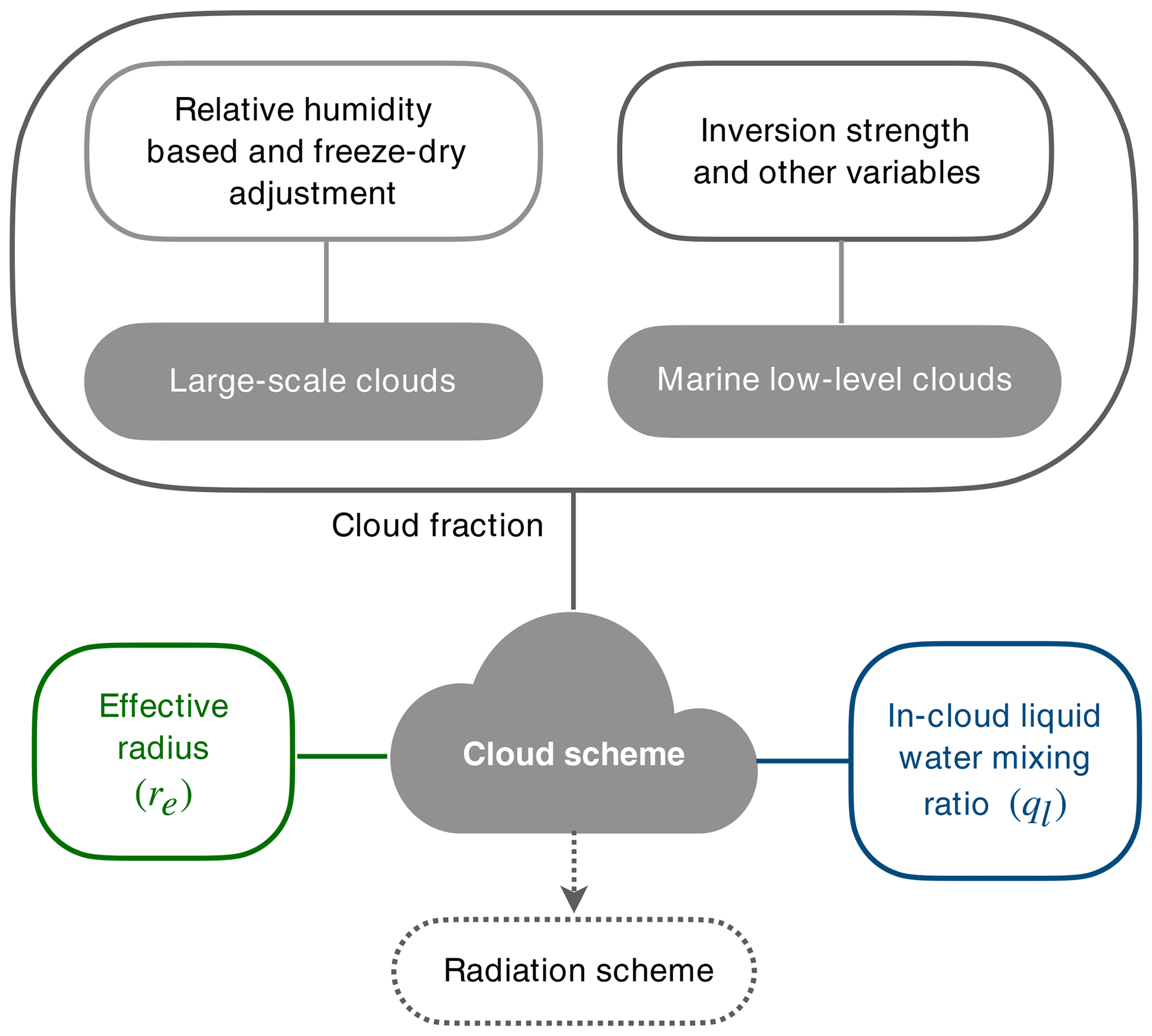
Figure 1A sketch of the SimCloud scheme components, which includes the cloud fraction, effective radius of cloud droplet and in-cloud liquid water mixing ratio. At any given location, the maximum of the cloud fractions from a large-scale cloud scheme and marine low stratocumulus cloud scheme is applied if both are used.
As noted in the introduction, large-scale clouds of SimCloud are parameterized as a function of relative humidity, and this provides the majority of the cloud cover. However, as discussed in Sect. 4, this scheme alone is found to be inadequate and two additional effects are needed. First, a “freeze-dry” method based on the specific humidity (discussed in Sect. 2.2.2) is used to reduce the large-scale cloud cover over polar regions to more realistic levels. Second, a separate marine low stratus cloud scheme (discussed in Sect. 2.2.3) is used to represent the stratiform clouds (which have a large shortwave radiative effect), and this has a particularly large effect in subtropical regions off the west coast of continents. These two additional components are optional, and users can decide whether to use them according to their research interest. Although these clouds have different physical properties (e.g., cloud top temperature), all of them are treated essentially as liquid clouds in our scheme. The effective radius of the cloud droplets is allowed to change with temperature, and this affects the radiative transfer. Some tuning of the cloud scheme is performed in order to fit the observations. Nevertheless, the values of certain parameters used in the scheme are not necessarily definitive and may be varied in order to examine the sensitivity of clouds to perturbations, such as CO2 increase.
The present version of the cloud scheme does not include a separate scheme for convective clouds, and the convection scheme in the model has no effect on cloudiness except in so far as it may change the relative humidity or possibly the low-level inversion. We find that the vertical structure of clouds can be simulated relatively well without explicit diagnosis of convective clouds (see Fig. 6), and we leave the possible explicit representation of convective clouds to a future study.
2.2 Cloud fraction
2.2.1 Relative humidity-based cloud fraction
The use of a relative humidity scheme is based on the notion that over a grid box the humidity varies and that condensation will occur and clouds will form even when the grid cell is not saturated (Tompkins, 2005; Quaas, 2012). One such scheme is that of Sundqvist et al. (1989), discussed more below. Such schemes do not account for variations in dynamical conditions except in so far as they are reflected in the relative humidity field, but they form a simple rational basis for cloud prediction. Here we implement two relative humidity schemes with different forms to diagnose the cloud fraction.
In the first scheme, the large-scale cloud fraction (Cs) is a piecewise linear function of grid-mean relative humidity (H), namely
The diagnosed cloud fraction is therefore unity when the mean relative humidity equal to one (i.e., the grid box is saturated). The value of a determines the critical value of relative humidity, Hc, above which clouds form, and thus and . The coefficient a (and hence Hc) is taken to be a function of height (or pressure) but not latitude or longitude.
The vertical profile of the coefficient a was derived from the reanalysis data sets. Specifically, the hourly relative humidity and cloud fraction data sets in year 2017 from the European Centre for Medium-Range Weather Forecasts (ECMWF) Reanalysis version 5 (ERA5) (Copernicus Climate Change Service (C3S), 2017) are used to derive the coefficient profile. Note that the saturated water vapor pressure is calculated over liquid and ice in ERA5 data set, while it is calculated over liquid only in the Isca simulations (see Sect. 3). We know this may lead to some discrepancies, but the linear coefficient a is tunable, which can make the parameters obtained from the reanalysis data set applicable to GCMs. The ERA5 has horizontal resolution and 37 vertical levels. For each vertical level, the piecewise linear relationship (as cloud fraction is not allowed to be smaller than 0 or larger than 1) is used to fit the cloud fraction against relative humidity with a least-squares method, and then the coefficient a of that level is obtained. In addition, we have re-gridded the data to three other horizontal resolutions, including , (T85) and (T42), to test whether the derived coefficient profile is sensitive to horizontal resolution. The derived profiles with different resolutions are shown in Fig. 2a, and the corresponding critical relative humidity (Hc) profiles are shown in Fig. 2b for reference. At a very high resolution, we would expect the humidity distribution in a given grid box to be narrower, and hence the critical value of relative humidity to increase; however, we find that the horizontal resolution has a relatively small influence on the coefficient profiles at the resolutions we consider here.
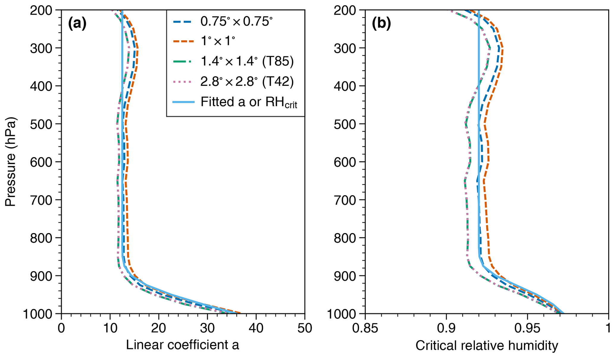
Figure 2(a) Vertical profiles of the linear coefficient for the relative humidity-based cloud diagnostic scheme, with cloud fraction as a piecewise linear function of relative humidity as shown in Eq. (1). The dashed lines with different colors are profiles of a obtained from ERA5 data with various horizontal resolutions. The solid pale blue line denotes the fitted profile used in the model based on the form of Eq. (2). Panel (b) is the same as (a) but for the critical relative humidity (Hc) profiles.
To apply the coefficient profile of a in the model, we use a profile similar to Quaas (2012) (see their Eq. 3):
where p is pressure, ps is the surface pressure, and as and at are the values of coefficient a at the surface and free troposphere, respectively. Such a functional form fits the observations fairly well with only a small number of tunable parameters. We use as=36, at=13 and n=12, which determines the shape of the profile. The fitted profile for a, as indicated by the solid pale blue line in Fig. 2, follows the reanalysis (dashed or dotted lines) quite well at low and middle levels but with some discrepancies at higher levels. The actual cloud fraction for each level is determined by Eq. (1) with the coefficient a for that level determined by Eq. (2).
We also provide the Sundqvist et al. (1989) scheme as another option for the relative humidity schemes, namely
where Hc is critical relative humidity. Here we specify Hc as a simple function of height, which is determined by critical relative humidity at three different levels: 0.95 at the surface, 0.85 at 700 hPa and 0.99 at 200 hPa, which are determined by running sensitivity tests. Between these levels, the critical relative humidity is linearly interpolated with height. To test the performance of the aforementioned schemes, we compare them with another linear scheme with a different form from Eq. (1), which is defined as
where a and b vary with height and are determined from the least-squares fitting of hourly cloud fraction and relative humidity data from ERA5 reanalysis. The cloud fraction in Fig. 3a is from ERA5 reanalysis at 450 hPa at 12:00 LT, 1 January 2017, while the cloud fractions from three schemes (Figs. 3b–d) are diagnosed from the ERA5 relative humidity field at the same time and level. The linear scheme defined in Eq. (4) has two tunable parameters, and thus one might expect it to perform better than the others. However, the cloud cover cannot reach 1 when the grid box is saturated (Fig. 3c), even though the spatial pattern of cloud cover resembles the ERA5 reanalysis and the global mean value is much closer to the ERA5 compared to the other two schemes. In contrast, the diagnosed cloud amount patterns from the Sundqvist scheme (Fig. 3b) and the linear scheme in the form of Eq. (1) (Fig. 3d) are quite similar to the reanalysis (Fig. 3a), although the cloud cover is a little overestimated in these two schemes. These offline tests suggest that the linear scheme in the form of Eq. (1) is promising to be applied in GCMs.
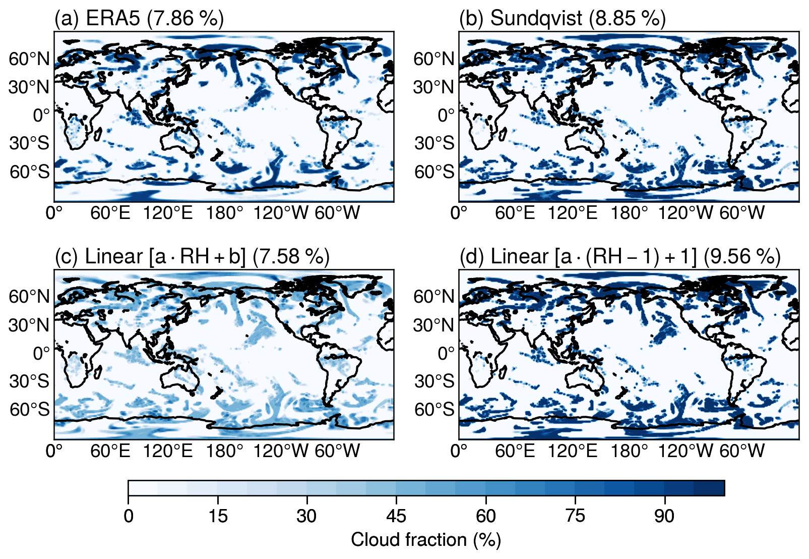
Figure 3(a) A snapshot of cloud fraction from ERA5 reanalysis at 450 hPa at 12:00 LT, 1 January 2017. Diagnosed cloud fraction from ERA5 relative humidity field at the same time and level based on the (b) Sundqvist formula and two linear formulas (c) using Eq. (4) and (d) using Eq. (1). Note that Eq. (1) is the form used to determine the large-scale clouds in this study. The global mean cloud fractions are given in the titles.
2.2.2 Freeze-dry adjustment
As we will show in Sect. 4.1, the cloud fraction and LW cloud radiative effect from the large-scale cloud scheme are overestimated in polar regions, especially during winter. The relative humidity-based cloud fraction scheme assumes there are subgrid-scale fluctuations of humidity and/or temperature, and thus the partial cloudiness is possible even under subsaturated conditions averaged over a grid box. However, this assumption might not be well suited for the extremely cold and dry atmospheric conditions in polar winter (Jones et al., 2004). The stable boundary layer condition in polar winter leads to little subgrid-scale spatial variability in humidity fields, and there should be less cloudiness than the turbulent environment for a given relative humidity. To alleviate this problem we implement a “freeze-dry” adjustment, a simple adjustment formula based on specific humidity from Vavrus and Waliser (2008) (see their Eq. 2). The freeze-dry adjustment is applied to reduce the cloud fraction under very dry conditions in polar regions. Specifically, if grid mean specific humidity (q) is below a threshold (qv), the cloud fraction (C) decreases linearly according to the water vapor content:
where f is the freeze-dry factor. Although the formula is applied globally, the threshold value in Eq. (5) ensures that only polar regions will be affected, and even in those regions the cloud fraction is adjusted only under very dry conditions.
In the original freeze-dry method, Eq. (5) was only applied in the lower troposphere (Vavrus and Waliser, 2008). In this study, the freeze-dry formula is applied through the whole atmospheric column, as this improves the cloud radiative effect in polar regions. In order to do so, we prescribe the specific humidity threshold qv in Eq. (5) to be a function of pressure with the threshold decreasing exponentially with height as
Here q0 is the surface specific humidity, ps is the sea level pressure (ps=1000 hPa) and n is the power to describe how quickly the specific humidity decreases with height. In Fig. 4, different profiles of qv are shown for the two tunable parameters n and q0. These two parameters are selected to ensure that the freeze-dry adjustment only has effects on polar regions when the qv profile is applied in Eq. (5). In doing so, the specific humidity profiles from several different regions are plotted in Fig. 4. In particular, the profiles at 60∘ N and 60∘ S are used to show the specific humidity boundary values of polar regions, and thus the two parameters q0 and n are tuned to follow the boundary profiles. As shown in Fig. 4, the qv profile follows the 60∘ N profile well when q0=0.006 kg kg−1 and n=2.5, which can also cover the specific humidity range poleward of 60∘ S. Therefore, in this study the parameters q0 and n are chosen as 0.006 kg kg−1 and 2.5, respectively. This threshold works well in current climate setup (see Sect. 4.1), but whether it holds under global warming situation still needs further investigation.
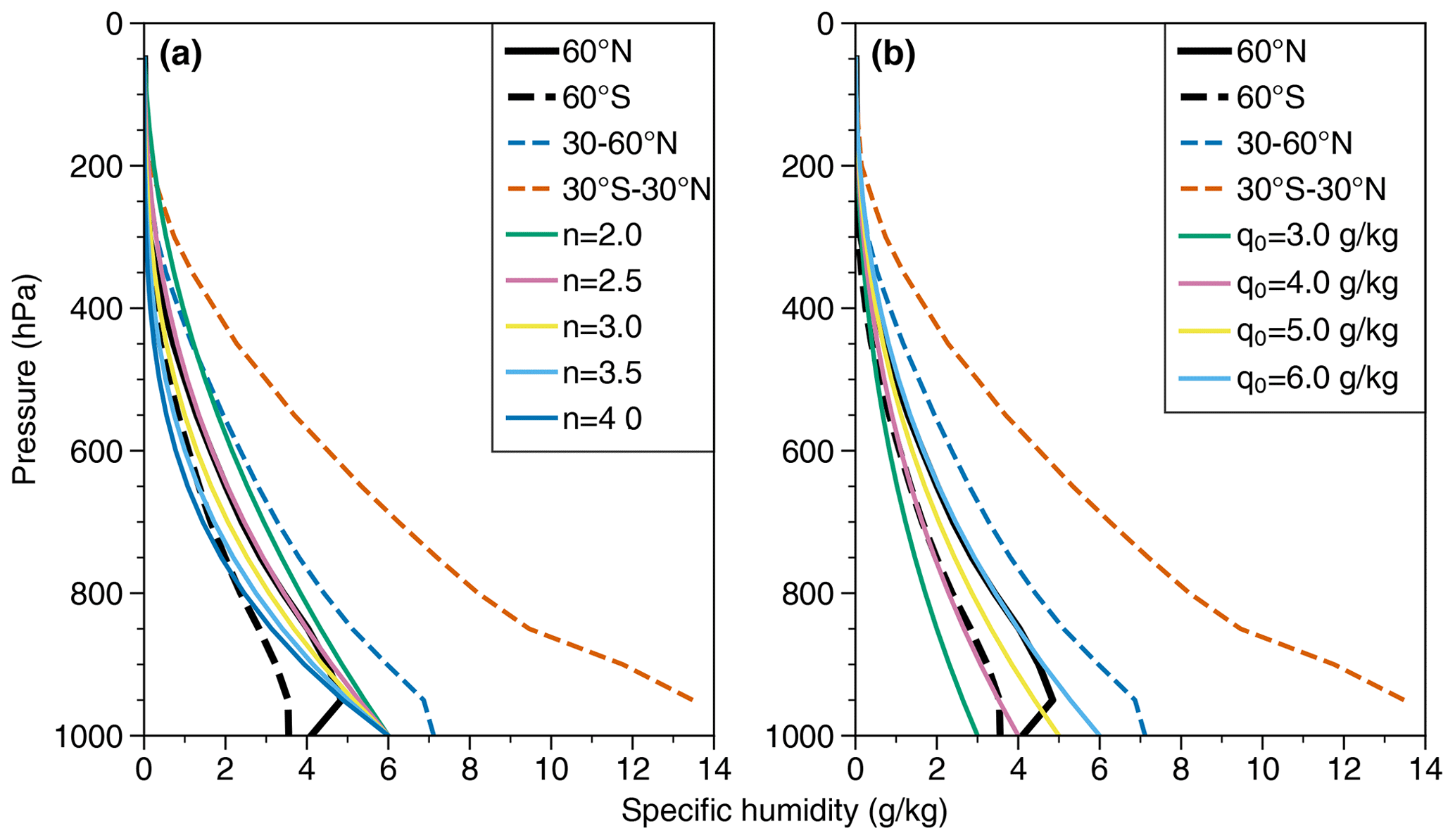
Figure 4The qv vertical profiles with different n and q0. The solid and dashed black lines are annual mean specific humidity profiles from the Isca simulation averaged over latitude circles, 60∘ N and 60∘ S, as boundary values of polar regions in the Northern Hemisphere and Southern Hemisphere, respectively. The dashed blue and orange lines are averaged specific humidity profiles over subtropical (30–60∘ N) and tropical (30∘ S–30∘ N) regions in the Isca simulation. The remaining solid lines are from Eq. (6) with different parameters. In the left panel, q0 in Eq. (6) is 0.006 kg kg−1, but n varies from 2 to 4. In the right panel, n=2.5 but q0 varies from 0.003 to 0.006 kg kg−1.
2.2.3 Low-cloud fraction
Low clouds, especially the subtropical marine stratocumulus clouds, are characterized by high albedo and a cooling effect on climate (Hartmann et al., 1992). Because these clouds cover about 20 % of the subtropical regions, even a small change in stratocumulus cloud amount can exert a large radiative forcing at the top of the atmosphere (TOA) (Slingo, 1990). However, marine stratocumulus amounts off the west coast of continents have commonly been underestimated, and this has been an issue in climate models for some time (e.g., Nam et al., 2012; Lauer and Hamilton, 2013; Dolinar et al., 2015).
Several proxies or indices for low-cloud fraction have been used as predictors for the stratocumulus clouds to try to remedy this (e.g., Kawai and Inoue, 2006; Joshi et al., 2015; Collins et al., 2004; Guo and Zhou, 2014; Kawai et al., 2019), including potential temperature lapse rate () of the most stable layer below 750 hPa (Slingo, 1987), lower tropospheric stability (LTS; Klein and Hartmann, 1993), estimated inversion strength (EIS; Wood and Bretherton, 2006) and the estimated cloud-top entrainment index (ECTEI; Kawai et al., 2017). Recently, Park and Shin (2019) proposed a new index, the estimated low-level cloud fraction (ELF), as a predictor for low-cloud fraction. ELF (which is a proxy and not necessarily a cloud amount itself) is defined as
where f is the freeze-dry factor defined in Eq. (5) with qv=0.003 kg kg−1 and q is the specific humidity of surface water vapor, zinv is the inversion height, zLCL is the lifting condensation level of near-surface air, and Δzs is a constant scale height (Δzs=2750 m). As shown by Park and Shin (2019), can be rewritten as , in which is a simple but practical proxy of surface moisture and quantifies the strength of the vertical decoupling of the inversion base air from the surface. The ELF predicts that low-level cloud fraction increases as the near-surface air gets more wet (smaller zLCL) and as the planetary boundary layer becomes more vertically coupled (smaller zinv).
We have examined the relationship between the seasonal mean low-cloud fraction and the various proxies (i.e., , LTS, EIS, ECTEI and ELF) using the ERA-Interim reanalysis data set (Dee et al., 2011). These proxies are derived from the 5-year monthly data from 2013 to 2017, including air temperature, surface pressure, surface temperature, and low-cloud fraction. As shown in Fig. 5, the regions with typical stratus clouds are selected for the calculation (Klein and Hartmann, 1993). The results indicate that the low-cloud fraction is linearly related to each indicator in stratus clouds regions, and the ELF tends to have very high correlation with the low-level cloud cover, judging from the fraction of variance (R2) explained by the regression equation. We thus choose to use ELF to construct the diagnostic low-cloud fraction formula, i.e.,
where Csc is the low stratus cloud fraction and the two coefficients b and c are treated as tunable parameters. The linear regression formula displayed in Fig. 5e provides a good starting point for tuning b and c in Eq. (8). After a sensitivity test performed with Isca (the setups will be introduced in Sect. 3), we find that if c is specified as the value shown in Fig. 5e, the shortwave cloud radiative effect is still weak compared to observations. Therefore, the parameters b and c are chosen as 1.3 and −0.1, respectively.
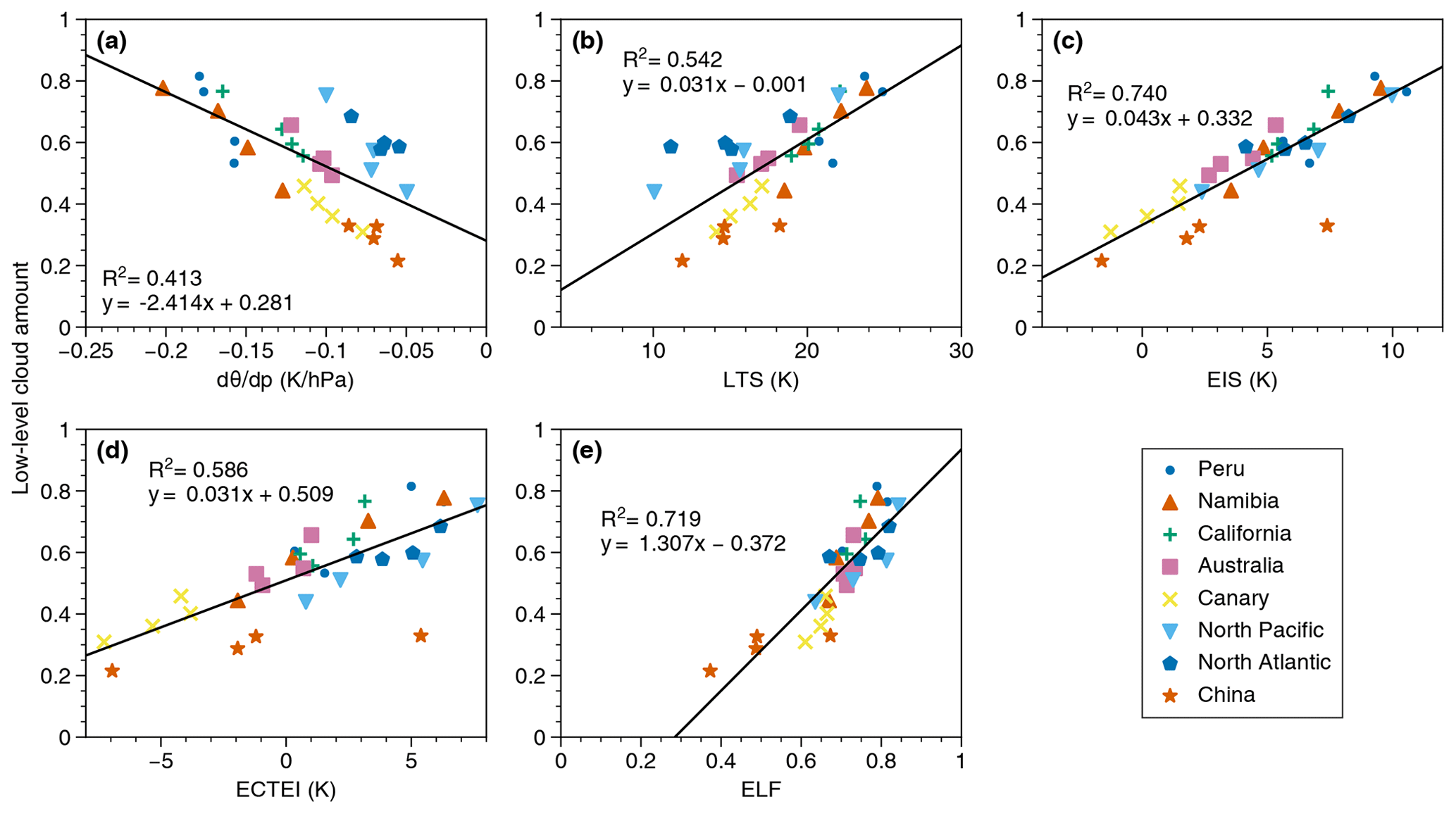
Figure 5The relationship between low-level cloud amount and (a) minimum below 750 hPa, (b) lower tropospheric stability (LTS), (c) estimated inversion strength (EIS), (d) estimated cloud-top entrainment index (ECTEI) and (e) estimated low-level cloud fraction (ELF) over stratiform cloud regions, including Peru (20∘ S–5∘ N, 80–90∘ W), Namibia (10–30∘ S, 0–15∘ E), California (15–30∘ N, 110–150∘ W), Australia (15–35∘ S, 90–110∘ E), the Canary Islands (15–25∘ N, 25–35∘ W), the North Pacific (40–50∘ N, 170–180∘ E), the North Atlantic (50–60∘ N, 35–45∘ W) and China (20–30∘ N, 105–120∘ E), which are selected based on Klein and Hartmann (1993). The data sets are from ERA-Interim reanalysis covering the period from 2013 to 2017. The four points in each region denote the average for different seasons. Linear regression lines and the corresponding fraction of variance (R2) explained by the equation are shown at the top of each plot.
In addition, the stratocumulus clouds usually form at the top of planetary boundary layer (Wood, 2012), where a strong inversion layer usually exists (Wood and Bretherton, 2006; Park and Shin, 2019). However, it is hard for a global model to capture the exact position of the inversion layer due to the limitation of vertical resolution (Kawai et al., 2019). Care thus needs to be taken to diagnose the marine stratocumulus clouds. First we find the most stable layer below 750 hPa, which is determined by the most negative (Slingo, 1987). Then within the most stable layer, if the lapse rate and vertical velocity satisfy K hPa−1 and ω>0 Pa s−1, respectively, then we diagnose stratocumulus clouds at that location. Note that the threshold is tuneable in our scheme, and it is −0.125 K hPa−1, as in Collins et al. (2004).
2.2.4 Cloud fraction diagnosis
The cloud fraction of a grid box (Ctotal) is simply defined as the largest fraction of all the clouds within that grid box for simplicity, without separate consideration of their different optical properties:
assuming a horizontal maximum overlap hypothesis (e.g., Collins et al., 2004; Roehrig et al., 2020). Cs and Csc in Eq. (9) are determined by Eqs. (1) and (8), respectively. To assess the performance of the cloud scheme, it is useful to evaluate the total cloud amount and cloud amounts at different levels. In our scheme, the cloud height is determined by cloud top pressure, where those located above 400 hPa are treated as high clouds, those below 700 hPa are defined as low clouds and in between are classified as middle clouds (Collins et al., 2004). Following this, the total, high, middle or low-cloud amounts are diagnosed from the maximum random overlap assumption (Morcrette and Jakob, 2000), which assumes maximum overlap for consecutive cloudy model levels and random overlap for cloud layers that are separated by clear-sky levels.
2.3 Effective radius and in-cloud water mixing ratio
Cloud particles, including liquid droplets and ice crystals, usually have different sizes, shapes and optical properties. In order not to introduce complicated microphysical processes, we do not distinguish them and assume that all particles seen by the radiation scheme are spherical liquid droplets and that ice clouds have a different effective radius from the liquid ones. In this study, the proportion of liquid cloud in a grid box varies with temperature, which only has an influence on the effective radius.
Following Ose (1993) and Boville et al. (2006), a very simple approach is used to represent the proportion of liquid cloud within a grid box (fl). Specifically, all clouds are assumed to be in liquid form if temperature is warmer than Tmax, and all the condensate is considered ice if the temperature is colder than Tmin. The cloud droplets are in the mixed phase at temperatures between Tmin and Tmax, and the proportion of liquid cloud in a grid box is defined as a linear function of temperature:
The bounds Tmin and Tmax are different in different models. For example, the lower bound (Tmin) is −40 ∘C in Ose (1993) and Boville et al. (2006), while it is −15 ∘C in Smith (1990). Observations have shown that cloud liquid water can exist at temperatures as low as −40 ∘C (Heymsfield and Miloshevich, 1993), although the incidence of liquid water in stratiform clouds is quite low at temperatures below −15 ∘C (Ryan, 1996). The upper bounds (Tmax) are −5 ∘C for stratiform clouds in Ose (1993), −10 ∘C in Boville et al. (2006) and 0 ∘C in Smith (1990). Based on the choices in previous studies, Tmin and Tmax in Eq. (10) are chosen to use −40 and −5 ∘C, respectively, in this study, but they are to be regarded as adjustable parameters.
The effective radius (re) of droplets within a grid box is defined as a weighted mean of liquid and ice particle radii, with the weights given by the liquid and ice cloud fraction, respectively. The radii of liquid and ice particles are selected based on observations. Stubenrauch et al. (2013) assessed cloud properties derived from various satellite data sets, finding that the global mean effective particle radii are about 14 (±1) and 25 (±2) µm for the tops of liquid clouds and for high-level ice clouds, respectively. Therefore, these two values are selected to calculate re,
which is applied globally in the model, although the effective radius of cloud droplets is found to be a little larger over ocean than over continents in observations (Stubenrauch et al., 2013).
The in-cloud liquid water mixing ratio (wl) is specified as a linear function of the atmospheric temperature, with values of g kg−1 at 220 K and wl0=0.18 g kg−1 at 280 K:
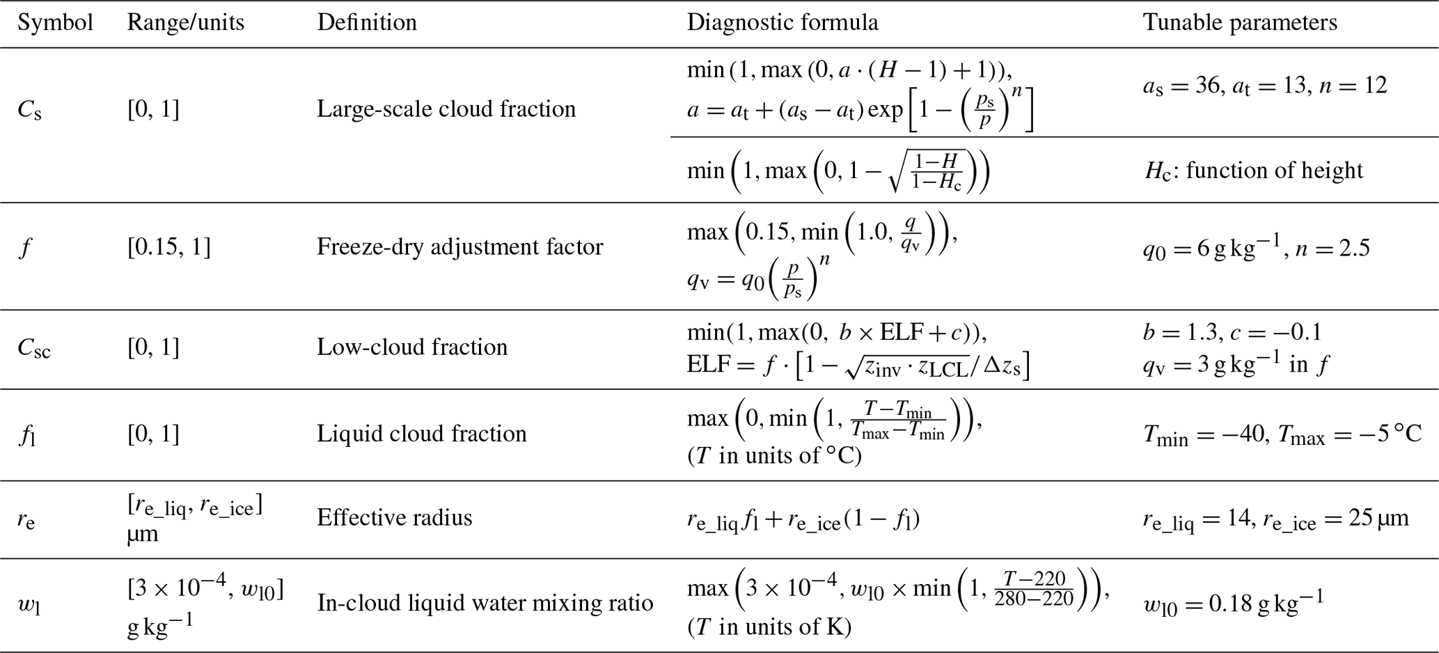
where the atmospheric temperature T is in units of K. The temperature thresholds, 280 and 220 K, are selected close to the global averages of liquid and ice cloud top temperature in observations, respectively (Fig. 4 in Stubenrauch et al., 2013). Thus, the grid mean liquid water specific humidity can be obtained from the product of wl and cloud fraction. Note that Eq. (12) is modified from the SPOOKIE II project (see https://www.cfmip.org/experiments/informal-experiments, last access: 1 May 2021, for detail). At first, the in-cloud water content is specified as a function of height, but in the second version of the protocol it has been updated as a function of temperature. For reference, the equations and parameters used in the cloud scheme are summarized in Table 1.
Table 1Summary of the simple diagnostic cloud scheme. Note that two options are provided for the large-scale cloud fraction (Cs).
The SimCloud scheme was implemented into Isca (Vallis et al., 2018) to examine its performance. Isca is an open-source framework for the construction of general circulation of atmospheres, which is built around a dynamical core from the Geophysical Fluid Dynamics Laboratory (GFDL) and physical parameterizations from Frierson et al. (2006) and Frierson (2007). Isca provides various options for users to set up experiments for their own interests, which include dry and moist models, various convection and radiation schemes, a variety of land–sea configurations and different parameters for other planetary atmospheres.
Our simulations are AMIP type; i.e., they follow those used in the Atmospheric Model Intercomparison Project. They are performed with a realistic Earth continental configuration following Thomson and Vallis (2018) (which is derived from the ERA-Interim land mask and topography, Dee et al., 2011) and at a horizontal resolution of T42 (roughly ) with 25 vertical levels. The monthly sea surface temperature and sea ice concentration are fixed at AMIP climatology (Taylor et al., 2000), derived from the input4MIPs data set (Durack et al., 2018) over the period from 1979 to 2008. The albedo in sea ice regions increases linearly with the sea ice concentration with the maximum of 0.7. The insolation includes a seasonal and diurnal cycle, with a solar constant of 1365 W m−2. The convection parameterization used in this study is the simplified Betts–Miller scheme from Frierson (2007), from which the convective precipitation is diagnosed. The large-scale precipitation is obtained from the large-scale condensation scheme (Frierson, 2007), which is accomplished by adjusting the humidity in supersaturated regions to the saturated values immediately, with temperatures adjusted to reflect this condensation. The SOCRATES (Suite Of Community RAdiative Transfer codes based on Edwards and Slingo) radiation scheme (Edwards and Slingo, 1996; Manners et al., 2015) is employed for the radiation transfer calculation as in Thomson and Vallis (2019). Spectral files with nine longwave bands and six shortwave bands are used, which are those used in the Unified Model's Global Atmosphere version 7 (Walters et al., 2019). The cloud fraction, effective radius of cloud particle and liquid water mixing ratio in each grid are passed to SOCRATES, and then the radiation fluxes under all-sky and clear-sky conditions are obtained, which are used to analyze the energy balance and to calculate the cloud radiative effect (Ramanathan et al., 1989; Li et al., 2017) at the TOA.
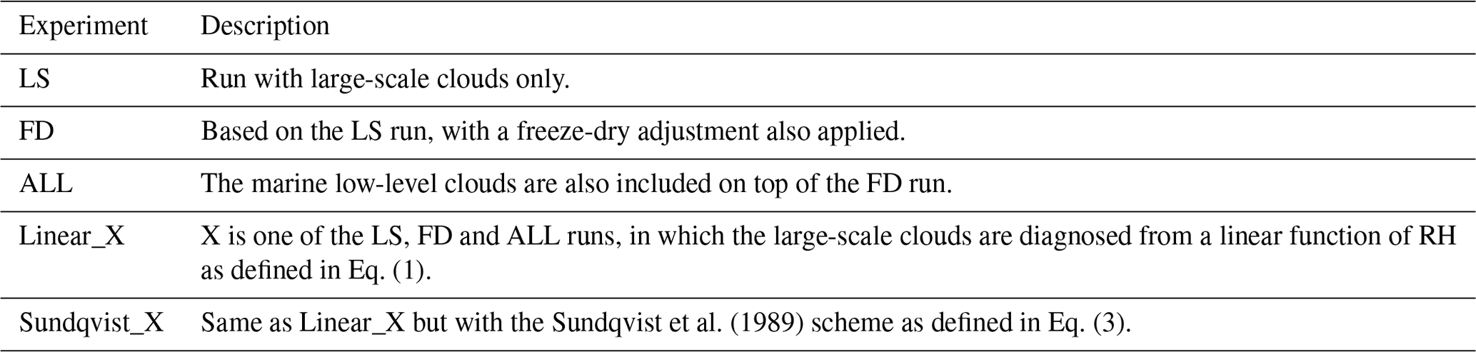
In order to compare the roles of different cloud parameterization schemes, simulations are performed with the combination of different clouds or different adjustment methods as shown in Table 2. The simulation with large-scale clouds only is denoted as the LS simulation. The run with large-scale clouds and freeze-dry adjustment is called the FD simulation. The run performed with large-scale clouds, freeze-dry adjustment and marine low stratiform clouds is referred to as the ALL simulation. The simulations are all run for 20 years, with the first 10 years treated as spin-up and discarded.
Sundqvist et al. (1989)Table 2Summary of the Isca fixed sea surface temperature (SST) simulations used in this study.
To evaluate the performance of the cloud scheme, several observations and reanalysis data sets are employed. Specifically, the cloud fraction from Isca simulations is compared to retrieved cloud fraction from GCM-Oriented Cloud-Aerosol Lidar and Infrared Pathfinder Satellite Observations Cloud Product (CALIPSO-GOCCP hereafter, 2007–2015; Chepfer et al., 2010). To examine the radiative flux simulated in Isca, monthly data from January 2001 to December 2018 from Clouds and Earth's Radiant Energy System (CERES) Energy Balanced and Filled (EBAF) Edition 4.1 product (CERES-EBAF hereafter; Loeb et al., 2018) are used for comparison. The cloud water path (sum of liquid and ice) is from the CloudSat 2B-CWC-RO Release P1_R05 data product (Austin et al., 2009) from 2012 to 2016, which can better represent cloud liquid and ice water path over high latitudes than CERES-EBAF data set, owing to its explicit determination of cloud phase (Lenaerts et al., 2017). In addition, monthly vertical velocity from ERA-Interim reanalysis and radiative flux data from CERES-EBAF data sets covering the period 2008–2017 are also adopted to quantify the LW CRE over the tropics.
In order to demonstrate how this cloud scheme performs with respect to more comprehensive models, the monthly mean radiative fluxes at clear-sky and all-sky conditions in historical simulations (1996 to 2005) from various CMIP5 models are also shown (see Fig. 17 for the names of models). All of the data sets are remapped to T42 resolution when necessary for a direct comparison with Isca simulations.
The global mean cloud amount and radiative components for the observations and Isca simulations are summarized in Table 3. We first focus on the mean state of the cloud amount, cloud water path and CRE at TOA from the LS, FD and ALL simulations (Sect. 4.1 to 4.3). Following this, in Sect. 4.4 we compare the simulated CRE with CMIP5 models. The sensitivity of the cloud scheme to the choice of parameters is briefly presented in Sect. 4.5.
Table 3Global and annual mean climatological properties of observations and different Isca simulations, which are summarized in Table 2. The net fluxes in the table are positive downward. The observed cloud amounts are from the CALIPSO-GOCCP data set (2007–2015), the radiative fluxes and cloud radiative effects (CREs) at the TOA are from the CERES-EBAF data set (2001–2018), and the cloud water path (sum of liquid and ice) is from the CloudSat data product.

4.1 Cloud amount
The global mean cloud fraction profiles from CALIPSO-GOCCP, ERA-Interim reanalysis and Isca simulations are displayed in Fig. 6a. The cloud fractions from all the Isca simulations are higher than observations, especially in the middle and high levels. The FD simulations are closer to observations than the LS simulations, which is true for both the linear and Sundqvist schemes. Regarding the annual and zonal mean profiles, a striking feature is that the LS simulations from both linear and Sundqvist schemes overestimate the cloud fraction at high latitudes (Fig. 6d and g) compared to the observation (Fig. 6b) and reanalysis (Fig. 6c). These biases are mitigated in the FD simulations (Fig. 6e and h), as the cloud fractions are limited due to insufficient water vapor content at high latitudes. Despite more clouds being diagnosed at low levels over the eastern subtropical ocean regions, the zonal mean cloud fraction profiles in the ALL simulations (Fig. 6f and i) are generally similar to those from the FD simulations. In summary, the cloud fraction profiles have been improved from the LS to ALL simulations due to the freeze-dry adjustment and the extra low clouds. However, the cloud fractions are still overestimated in high levels over the subtropics, which could possibly explain the CRE biases over these regions.
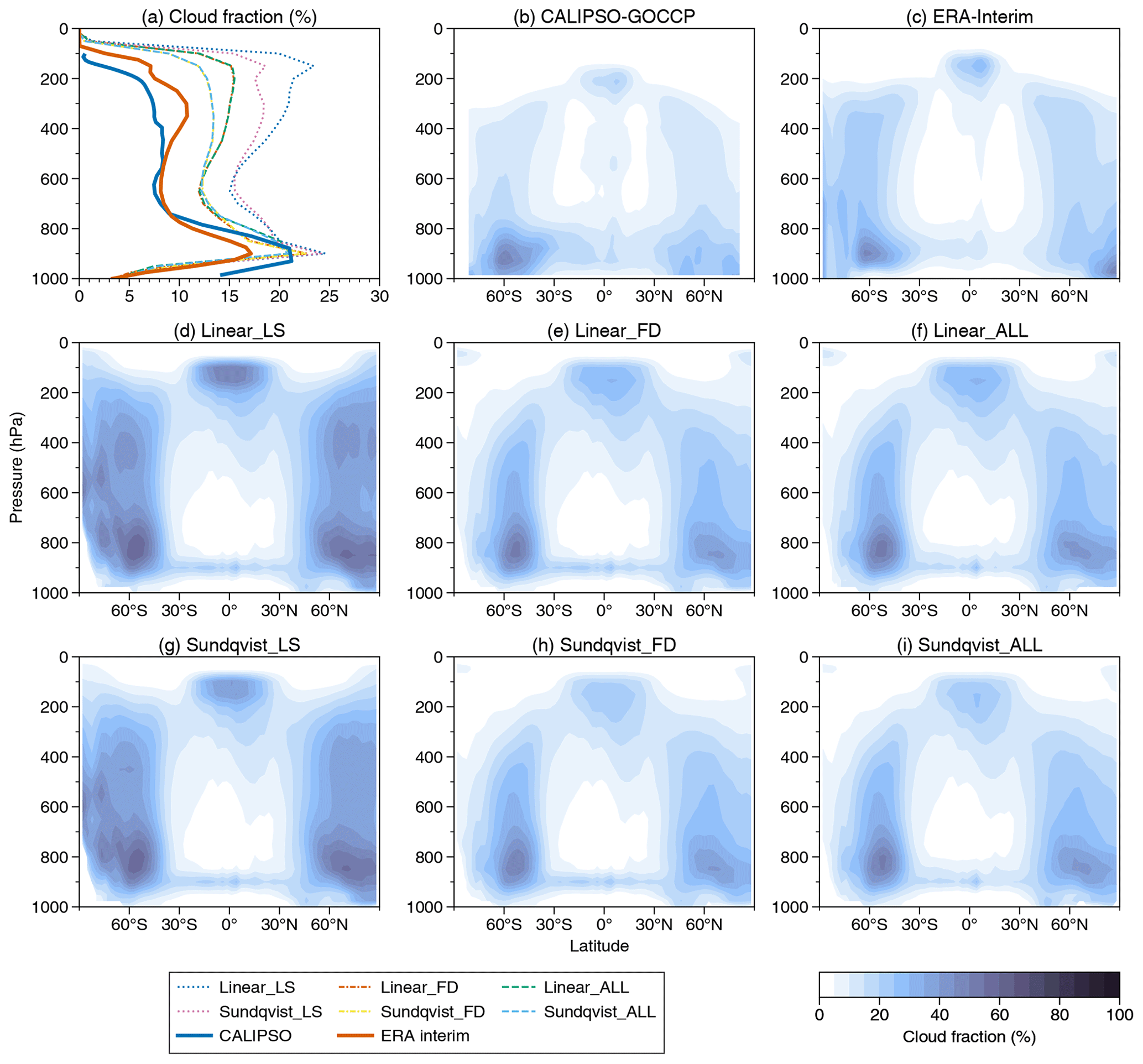
Figure 6(a) The annual and global mean of cloud fraction profiles from the CALIPSO-GOCCP (thick solid blue line), ERA-Interim reanalysis (thick solid orange line) and different Isca simulations, including linear_LS (dotted blue), linear_FD (dash-dotted orange), linear_ALL (dashed green), Sundqvist_LS (dotted pink), Sundqvist_FD (dash-dotted yellow) and Sundqvist_ALL (dashed azure). (b–i) The same as in (a) but for annual and zonal mean of cloud fraction profiles.
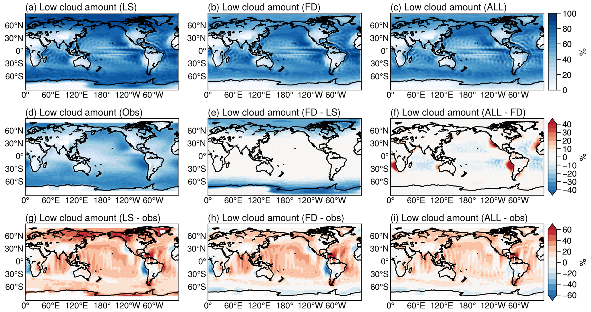
Figure 7The annual mean geographic patterns of low-cloud amount (%) from the (a) LS, (b) FD, (c) ALL simulations with the linear scheme and (d) observation (CALIPSO-GOCCP), and the differences between the (e) FD and LS, (f) ALL and FD, (g) LS and observation, (h) FD and observation, and (i) ALL and observation. Note that (a–d) use the upper color scale, (e–f) use the middle one, and (g–i) use the one at the bottom.
In addition to the cloud fraction profiles, the geographic patterns of cloud amount, diagnosed from the maximum random overlap assumption (Sect. 2.2.4), are also compared with observations. For example, the annual mean spatial patterns of low-cloud amount from three different simulations (LS, FD and ALL) with a linear RH cloud scheme, the CALIPSO-GOCCP data set and the differences between them are shown in Fig. 7. It should be pointed out that in this study we do not compare the simulated cloud amount with satellite retrievals directly, as the cloud simulator (e.g., Bodas-Salcedo et al., 2011) has not been implemented in Isca.
One evident feature of the low-cloud amount in observations is that marine stratocumulus clouds dominate the areas off the west coast of continents (Fig. 7d), related to the subsiding branch of the Hadley cell (Wood, 2012). The predominantly downward motion in these regions generally suppresses cloud formation in the middle and upper troposphere, but due to the abundance of water vapor near the ocean surface, clouds form at the top of convective boundary layers. However, these marine low clouds are too far from the coasts in the LS simulation compared to the observations (Fig. 7a). Looking at the differences between LS simulation and observations (Fig. 7g), the low-cloud amount is underestimated by about 20 % off the west coast of Peru. In fact, these are well-known biases in CMIP5 models (Dolinar et al., 2015). Another problem of the LS simulation is the overproduction of low-cloud amount in polar regions (Fig. 7g). For example, LS simulation produces more than 40 % low cloud over Arctic region.
In contrast, the cloud fractions in the FD and ALL simulations are adjusted by the freeze-dry method (see Sect. 2.2.2), which is mainly designed to reduce the unrealistic cloud amount in polar regions. Thus, there is a reduction of low-cloud amount over high latitudes in these two simulations (Fig. 7h and i), although some positive biases still exist there. Compared with the LS simulation directly, the FD simulation can reduce the low-cloud amount by more than 20 % over polar regions (Fig. 7e), showing a better agreement with the observations. The ALL simulation can further diagnose the marine stratus clouds off the west coast of continents through the predictor ELF, making the distribution of low clouds closer to the observation (Fig. 7c). It is noted that pronounced changes occur off the west coasts of Peru, California and Namibia in the ALL simulation, where the cloud fraction increases over 20 % (Fig. 7f) compared to the FD run. As shown in Table 3, the global mean low-cloud amount decreases from 54.9 % to 48.8 % from the LS to ALL simulations with the linear RH scheme, which is closer to the observed value (40.4 %). The changes of total cloud amount in these simulations (not shown here) are similar, and the global mean value decreases from 76.4 % (the LS run) to 66.5 % (the ALL run) for the linear RH scheme (Table 3).
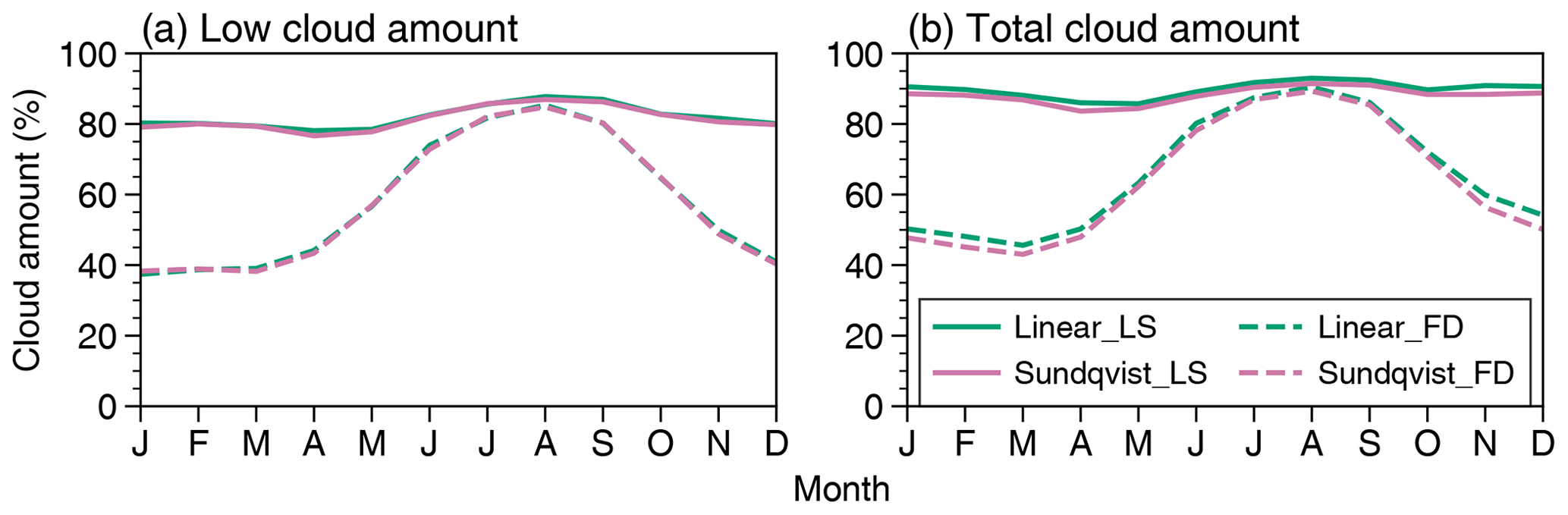
Figure 8The seasonal cycle of (a) low and (b) total cloud amount (%) over the Arctic region (60–90∘ N) from the LS (solid lines) and FD (dashed lines) simulations, where the freeze-dry adjustment method is applied in the FD simulations. The green and pink colors denote the experiments performed with the linear and Sundqvist cloud schemes, respectively.
The above analyses have shown that the freeze-dry method can improve the spatial patterns of annual mean cloud amount, with these changes being especially pronounced during winter (as also noted by Vavrus and Waliser, 2008). Figure 8 illustrates the annual cycle of low and total cloud amounts over Arctic region from both linear RH and Sundqvist schemes. In the LS simulations, both the low and total cloud amounts are nearly at the same level throughout the year. However, a striking feature in the FD simulations is that the cloudiness declines rapidly during boreal winter but remains almost unchanged in warm and moist summer, which in fact is more realistic compared to observations, as pointed out by Vavrus and Waliser (2008).
4.2 Cloud water path
The cloud water path (CWP) measures the total amount of cloud water within a column and is defined as the integral of cloud water content from the surface (p=ps) to TOA (p=0) (Eq. 9.30 in Stensrud, 2007), and it can be expressed as follows if the hydrostatic equilibrium is assumed:
where wl is the in-cloud liquid water mixing ratio specified in Eq. (12), C is the cloud fraction within a grid box, g is the acceleration due to gravity and p is the pressure. The global and annual mean CWP in the LS simulation from linear RH scheme is 142.1 g m−2, which is larger than the observed global mean result (119.3 g m−2; see Table 3). As displayed in Fig. 9, one obvious bias in the spatial pattern in the LS simulation is the overestimation of CWP at high latitudes. For instance, these biases can be even more than 90 g m−2 in the polar regions (Figs. 9a and g). As the simple cloud scheme neglects the ice and mixed-phase microphysics, this may contribute to the overestimate of CWP. Such an overestimation is also evident in cloud amount over polar regions (e.g., Fig. 7g), suggesting that the adjustment of cloud fraction probably reduces the CWP biases there. Indeed, incorporating the freeze-dry method into the simulation produces a large change in the CWP spatial pattern, with a reduction of over 60 g m−2 over polar regions (Fig. 9b, e and h). The CWP biases off the west coast of continents are reduced in the ALL simulation due to the increase in the low-cloud fraction there. For example, the CWP over the Peruvian and Californian coasts in the ALL simulation increases at least 20 g m−2 when compared to the LS simulation (Fig. 9e and f).
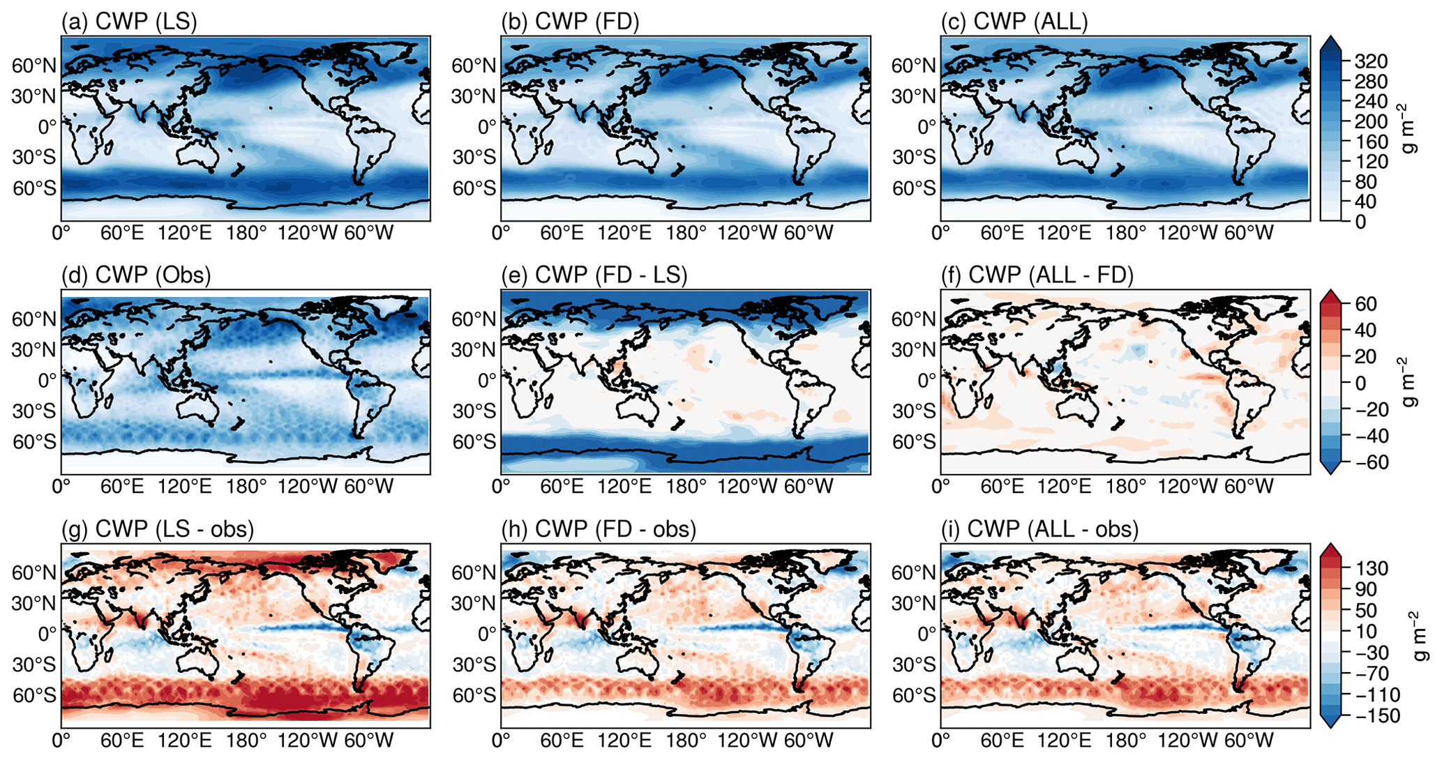
Figure 9The same as Fig. 7 but for the spatial patterns of total cloud water path (CWP; g m−2). The observed climatology of CWP is derived from the CloudSat data set.
4.3 Cloud radiative effect at TOA
The CRE is defined as the differences in TOA radiative fluxes between clear-sky and all-sky conditions (e.g., Ramanathan et al., 1989; Li et al., 2017). Specifically, the simulated LW CRE is derived from the difference between the outgoing longwave radiation flux under clear-sky and all-sky conditions, and the SW CRE is computed from the difference in reflected SW flux under clear-sky and all-sky conditions. The net CRE is defined as the sum of LW and SW CREs.

Figure 10The same as Fig. 7 but for shortwave (SW) cloud radiative effect (CRE; W m−2) at TOA. The observed SW CRE is from the CERES-EBAF data set.
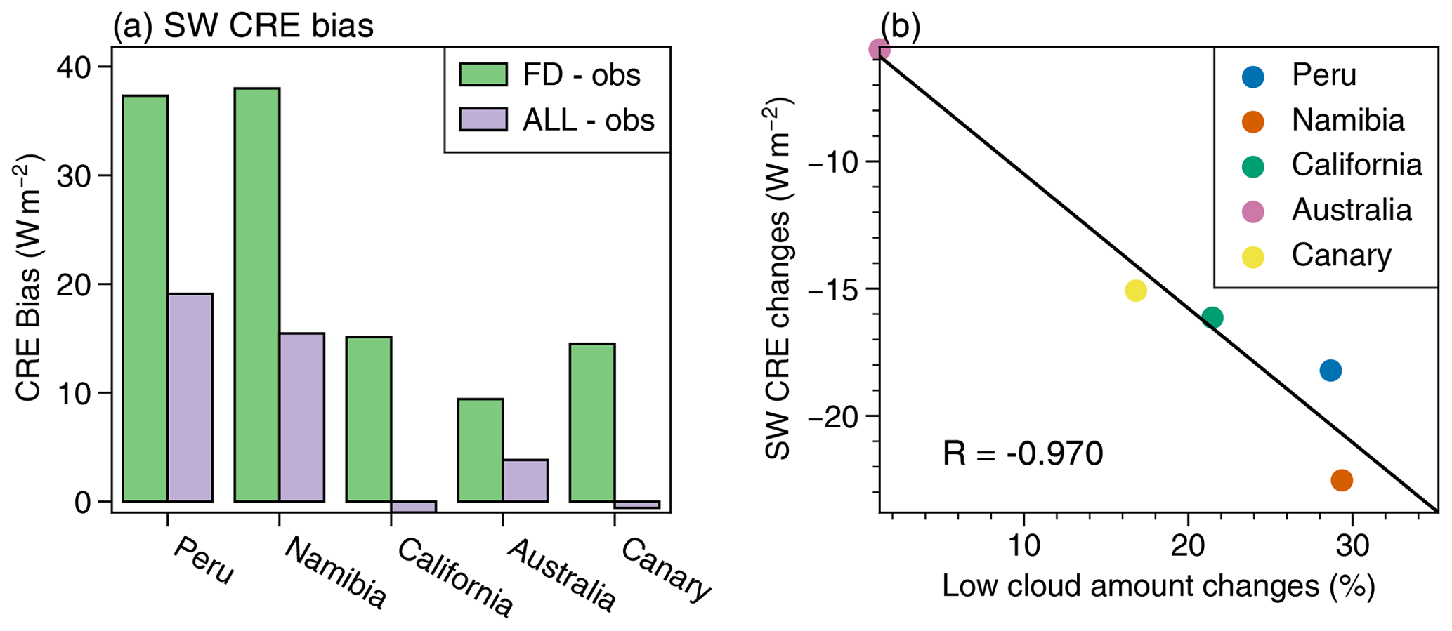
Figure 11(a) The regional mean SW CRE biases from the FD and ALL simulations with the linear RH scheme in five different subtropical ocean regions off the west coast of continents, whose ranges are defined in the caption of Fig. 5. (b) The relationship of regional mean SW CRE and low-cloud amount changes in the FD and ALL simulations; the changes are calculated as their differences (i.e., ALL-FD).
4.3.1 Spatial patterns of cloud radiative effect
The global mean SW CRE from the LS simulation is −60.0 W m−2, which is much larger than the observed value of −45.8 W m−2 from CERES-EBAF (Table 3). Compared to the observed SW CRE (Fig. 10d), the LS simulation can reproduce the general features of spatial patterns (Fig. 10a), although it fails to grasp some key features. For example, SW CRE is underestimated by over 30 W m−2 in eastern subtropical ocean basins off the west coast of Peru and over 15 W m−2 off the west coast of California (Fig. 10g), consistent with the insufficient low-cloud amounts in these marine stratocumulus areas (Fig. 7g). These biases also exist in the FD simulation (Fig. 10b and h), as the freeze-dry method can only adjust the cloud amount over high latitudes. As shown in Sect. 4.1 and 4.2, the low-cloud amount and CWP in these regions increase in the ALL simulation, which is thus expected to improve the SW CRE biases. In fact, the differences between the ALL and FD simulations show that the SW CREs reduce by more than 10 W m−2 off the Californian, Peruvian and Namibian coasts (Fig. 10f). Consequently, the positive biases in SW CRE over eastern subtropical ocean regions are reduced, although some smaller positive biases still remain (Fig. 10i). The SW CRE biases from the FD and ALL simulations in the five marine stratocumulus clouds regions (defined in Fig. 5) are quantified in Fig. 11a. It is clear that these biases are reduced in all of the locations, and this is closely linked to the increase in low-cloud amount over these regions (Fig. 11b).
Another problem of the SW CRE in the LS simulation is that it is too negative in trade wind cumulus regions, i.e., the Southern Ocean and northern Pacific Ocean (Fig. 10g), which is associated with the excessive clouds over these regions (Fig. 7g). The freeze-dry adjustment has reduced the cloud amount at high latitudes, making the SW CRE in the Southern Ocean less negative compared to the LS simulation (Fig. 10e and h). In the end, the spatial pattern of SW CRE in the ALL simulation becomes more realistic compared to observations, but we also notice that the global mean SW CRE bias is still about 10 W m−2 compared to the observed value (−45.8 W m−2) from CERES-EBAF (Table 3), implying that some errors still exist in microphysical properties (e.g., effective radius) and/or other processes in the model in addition to the macrophysical properties (e.g., cloud fraction).
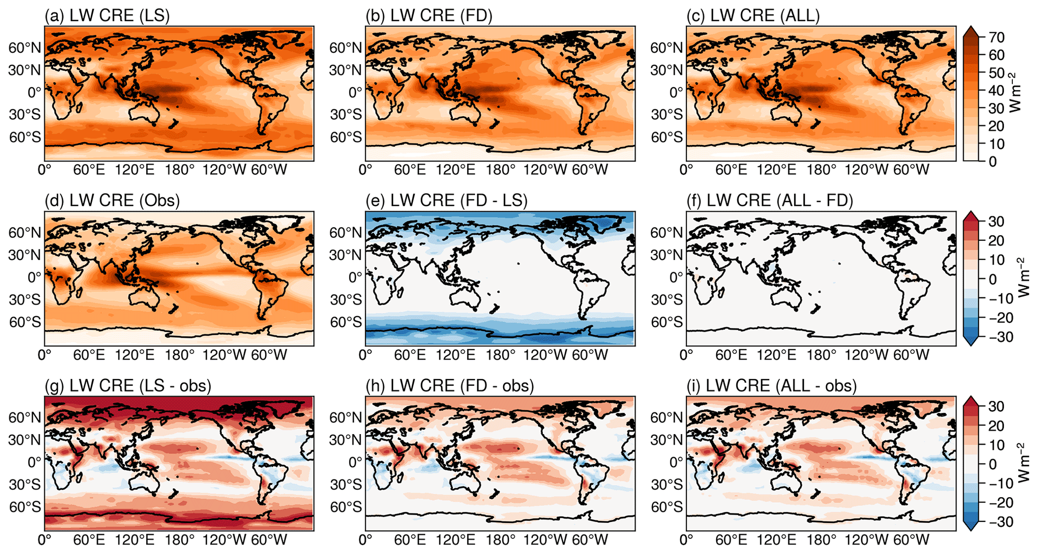
Figure 12The same as in Fig. 10 but for LW CRE (W m−2) at TOA.
The LS simulation reproduces the general spatial pattern of the observed LW CRE (Fig. 12a and d). However, the radiative effect is too strong, especially in the polar regions and also over the subtropical oceans located east of the Maritime Continent (Fig. 12a and d), which is also illustrated by the positive biases over these regions (Fig. 12g). The LW CRE in the LS simulation is overestimated by over 30 W m−2 in the Arctic and over 15 W m−2 in tropical regions. As discussed in previous sections, the cloud fraction, as well as the CWP in polar regions, decreases in the FD simulation compared to the LS run. Therefore, the LW CRE is improved over these regions (Fig. 12b and h), where the bias in polar region is reduced by more than 15 W m−2 (Fig. 12e). Nevertheless, there is still a small positive bias over the Arctic and tropical regions. Compared to the FD simulation, the changes in the ALL simulation has little effect on LW CRE (Fig. 12f). After these improvements, the spatial patterns of LW CRE in the FD and ALL simulations become more similar to the observations, and the global mean CRE drops from 36.8 to 31.6 W m−2, much closer to global mean result from observations (Table 3).
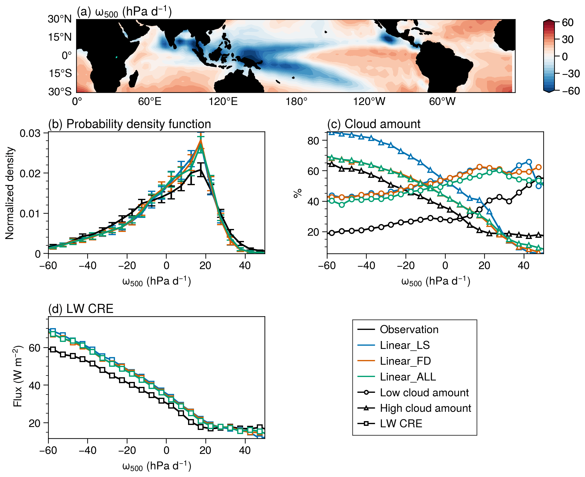
Figure 13(a) The vertical pressure velocity field at 500 hPa (ω500) over tropical oceans between 30∘ S and 30∘ N from the linear_LS simulation. (b) The probability density functions (PDFs) of the 500 hPa large-scale vertical velocity (ω500) over the tropical ocean regions defined in (a), where the vertical bars indicate 1 standard deviation of the annual mean data. (c) The low and high cloud amounts and (d) the TOA LW CRE in different dynamical regimes binned by ω500. The 9-year (2007–2015) observed cloud amounts from CALIPSO-GOCCP and the LW CRE from CERES-EBAF are binned by ω500 from ERA-Interim reanalysis data set (black lines). The results from the LS, FD and ALL simulations with the linear RH scheme are represented by blue, orange and green lines, respectively.
To further quantify the simulated LW CRE at TOA over the tropical ocean regions (30∘ S–30∘ N), following the method employed in Bony et al. (2004) and Bony and Dufresne (2005), we first define the upwelling and downwelling regimes based on the vertical pressure velocity at 500 hPa (ω500, Fig. 13a), and then evaluate the LW CRE over these regimes. ω500 is a measure of the large-scale atmospheric circulation, where the regions with positive ω500 are associated with the descent, while those with negative ω500 are related to large-scale atmospheric ascent. The PDFs of ω500 from the ERA-Interim reanalysis and Isca simulations (LS, FD and ALL runs) are displayed in Fig. 13b. The PDFs of the Isca simulations generally follow the observations, although the Isca simulations have fewer weakly ascending regions and more weakly descending regions. The peak values of PDFs are located at 5–20 hPa d−1, consistent with the results from Bony et al. (2004).
Figure 13c and d illustrate the high- and low-cloud amounts and LW CRE at the TOA over different dynamical regimes over tropical oceans, respectively. The observed cloud amount and LW CRE are from CALIPSO-GOCCP and CERES-EBAF data sets, respectively, both covering the period from 2005 to 2014 with the regimes being defined by the ω500 from ERA-Interim. The regimes with stronger convective activity, related to the magnitude of ω500 in ascending regions (ω500<0), usually have a larger amount of high clouds and thus stronger LW CREs. All the LW CREs from the three simulations are close to the observed values over the weak upwelling and subsidence regions. However, the LW CREs from the LS simulation deviate from the observations in strongly ascending regions ( hPa d−1). Furthermore, this discrepancy increases with the magnitude of ω500 in ascending regions (ω500<0). It is noted that the large biases of LW CRE over ascending regions is reduced slightly in the FD and ALL simulations, associated with the decrease in high clouds over those regimes (Fig. 13c). However, the positive biases still exist at the strong convection regions.
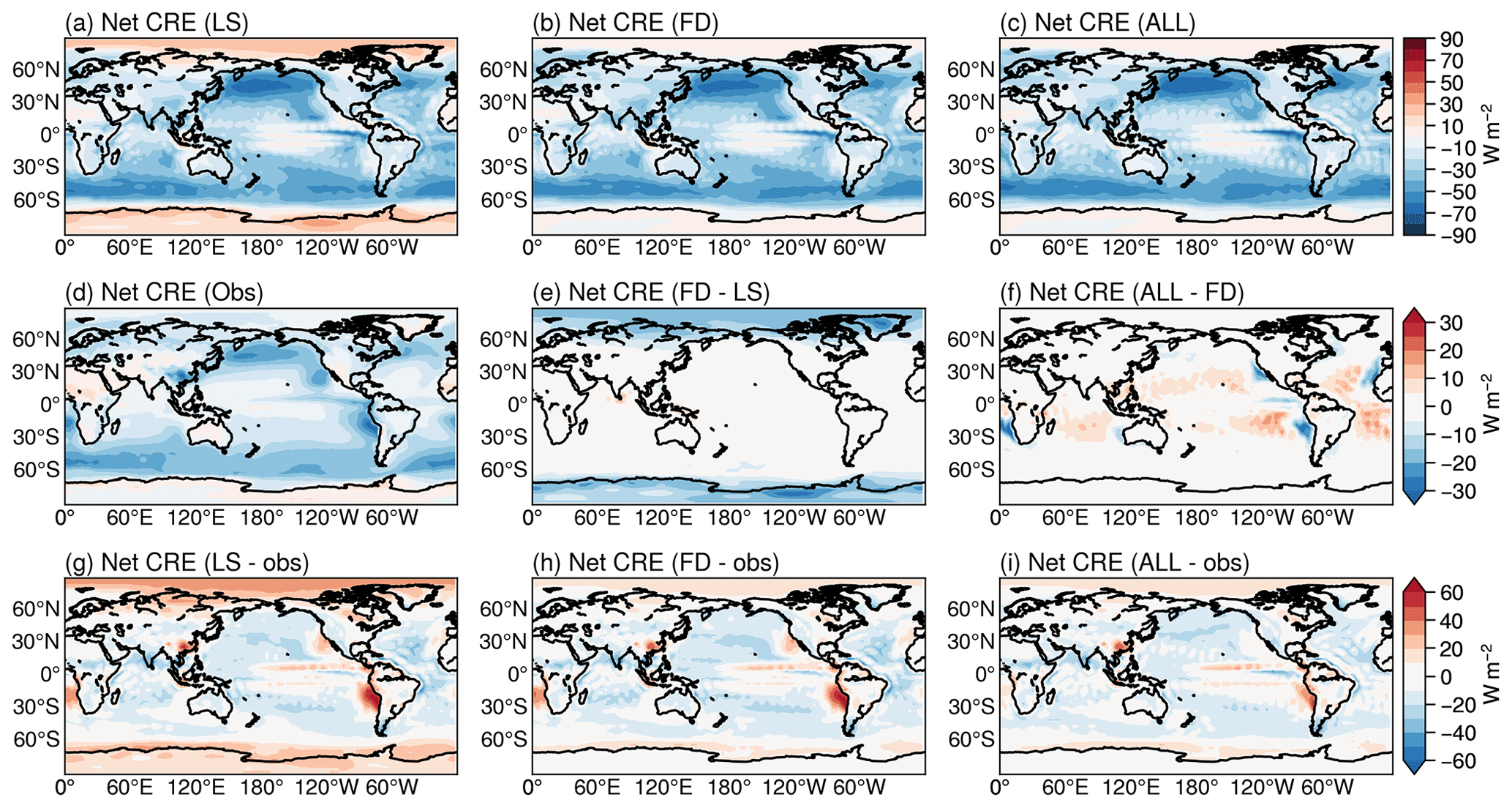
Figure 14The same as in Fig. 10 but for net CRE (W m−2) at TOA.
Finally, the spatial patterns of net CREs at the TOA are presented in Fig. 14, where we can see that the positive biases in the LS simulation mainly occur in the polar regions and subtropical eastern ocean regions. There are also small negative biases in subtropical and extratropical regions. The positive biases in net CRE in the LS simulation are related to the cloud amount biases in these regions, as we have seen in the SW and LW CRE fields. Clearly, the biases in polar regions are reduced greatly in the FD simulations (Fig. 14b, e and h) due to the freeze-dry method. Additionally, the positive biases off the west coasts of continents in subtropics can be mitigated in the ALL simulation (Fig. 14i), making the spatial pattern closer to CERES-EBAF, although there are still slight positive biases in polar regions.
4.3.2 Zonal mean structure
To further study their latitudinal variations, the zonally averaged SW, LW and net CREs from Isca simulations, CMIP5 simulations, satellite observation and the reanalysis data set are shown in Fig. 15. For the SW CRE (Fig. 15a), the general latitudinal variations can be captured by all of the Isca simulations, but the magnitude is larger than observations. The largest discrepancy in the LS simulations occurs in the mid-latitudes, especially in the Southern Hemisphere, which is likely arising from the excessive cloud amount over these regions (Fig. 7g). The improvement of cloud amount biases in the FD and ALL simulations contributes to the improvement of SW CRE over the extratropics. However, the difference in zonal mean SW CREs between the FD and ALL simulations is small, although the SW CRE biases over eastern subtropical ocean regions are reduced in the ALL run (Fig. 10f). In addition, the remaining SW CRE biases, as well as the low-cloud amount biases, in the ALL simulation over the subtropics and extratropics might be alleviated by an “omega correction”, namely a reduction of the low-cloud fraction if subsidence is strong (e.g., Gordon, 1992), but the effects are mixed, and we do not include that process in these results.
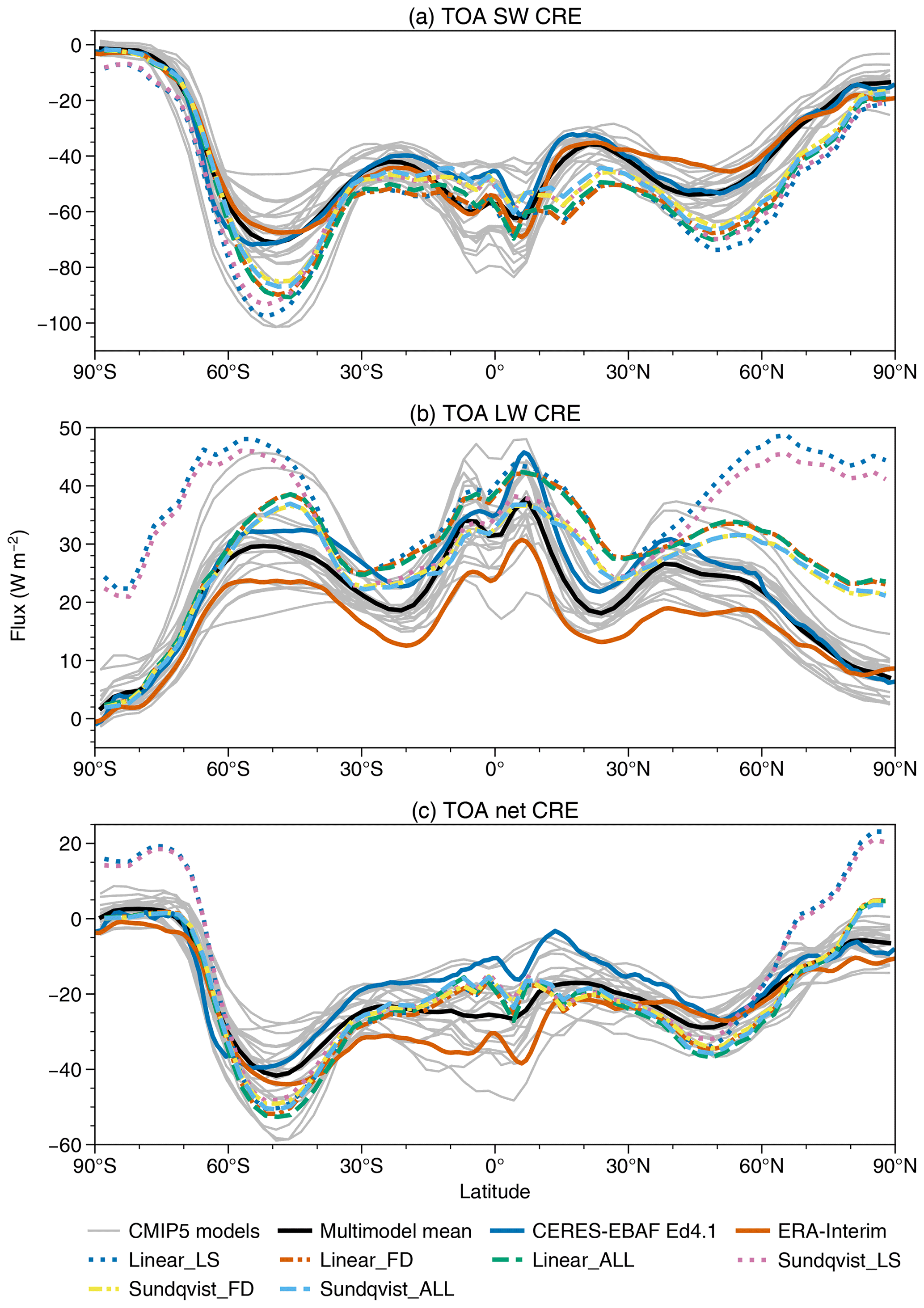
Figure 15Zonally averaged distribution of the TOA (a) SW, (b) LW and (c) net CREs from CERES-EBAF Ed4.1 (solid blue line), ERA-Interim reanalysis (solid orange line), CMIP5 models (thin, solid gray lines for each model and solid black line for multimodel mean) and different Isca simulations (dashed or dotted colored lines, listed in legend).
The LS simulations with both the linear RH and Sundqvist schemes agree well with observations of LW CRE at low latitudes (Fig. 15b). However, there are large discrepancies from the observations in the middle to high latitudes, which is consistent with the large biases of cloud amount at high latitudes (Fig. 6d and g). It is striking that these biases can be largely reduced through the freeze-dry adjustment, as the LW CREs agree much better with the observation at high latitudes in the FD and ALL simulations. The remaining deviation from observation in Isca simulations over Arctic region is possibly associated with the simple sea ice setup in our model. Likewise, the disagreement between zonal mean net CREs at high latitudes between the LS run and the observations almost disappears in the FD and ALL runs (Fig. 15c).
In addition, compared to the zonal mean variation of the SW, LW and net CREs from CMIP5 models, the Isca simulations are generally located within the spread of CMIP5 simulations at each latitude, except for the LW and net CREs over high latitudes in the LS simulations (Fig. 15b and c). These biases are alleviated in the FD and ALL simulations, although there are still some discrepancies over Arctic regions.
4.3.3 Seasonal cycle
The zonal mean seasonal cycles of CREs from the CERES-EBAF and Isca simulations (LS and ALL) with the linear RH scheme are displayed in Fig. 16. In the Arctic region, the observed LW CRE is weak during boreal winter and early spring and has a maximum in summer (Fig. 16a). The simulated LW CRE tends to be overestimated throughout the year in the LS run (Fig. 16b), but the biases are alleviated by the freeze-dry adjustment (in the ALL run), particularly in winter (also see Fig. 8), leading to an overall improvement in the representation of the high-latitude seasonal cycle of the CRE. The existing problem for the seasonal cycle of LW CRE is that the band in tropical region is too broad compared to the observations, which might relate to the too-broad high cloud pattern in tropical and subtropical regions (see Fig. 6f).
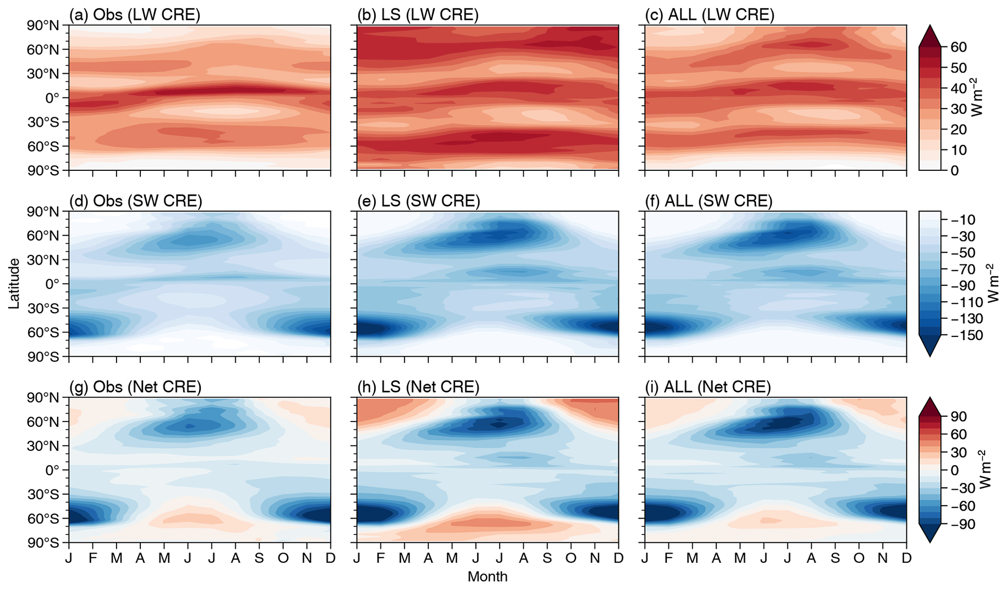
Figure 16The zonal mean annual cycle of TOA LW (a, b, c), SW (d, e, f) and net (g, h, i) CREs from observation (CERES-EBAF), LS and ALL simulations with the linear RH scheme in Isca.
The seasonal cycle of SW CRE in the LS simulation is realistic, except that it is too strong during boreal summer near 60∘ N (Fig. 16d and e). This effect is slightly mitigated in the ALL simulation (Fig. 16f) because of the improvement of cloud amount. Similar to the LW CRE, the positive biases of net CRE in winter over polar regions are also alleviated due to the improvement of LW CRE in winter (Fig. 16h and i). In summary, the seasonal cycles of LW, SW and net CREs in simulations with freeze-dry and inversion-based adjustments compare well to observations (left and right columns of Fig. 16), indicating that the cloud scheme does reproduce a reasonably realistic seasonal cycle of CREs.
4.4 Comparison of CREs with CMIP5 models
To evaluate the simulated CREs further, Isca simulations are compared with CMIP5 models. Figure 17 shows the global mean TOA SW, LW and net CREs from 21 CMIP5 models and Isca simulations with different cloud scheme setups. The observed SW CREs from CERES-EBAF and the multimodel mean of CMIP5 models are −45 and −48.3 W m−2, respectively. While the multimodel mean SW CRE shows small difference from the observation, the spread among these CMIP5 models is large. Compared to the observation and CMIP5 models, the global mean SW CREs from the LS simulations with the linear RH and Sundqvist schemes are too strong but are more realistic in the FD and ALL simulations. With all components of our simple cloud scheme (ALL simulation), the global mean values are −57.3 and −52.8 W m−2 for linear RH and Sundqvist schemes, respectively, which are fairly close to the observed and multimodel mean values. The changes of LW CRE from the LS to ALL simulations are similar to SW CRE, where the LW CRE drops from 36.8 to 31.6 W m−2 for linear RH scheme and decreases from 33.3 to 28.3 W m−2 for Sundqvist scheme, making the results from the simple cloud scheme closer to observations. These changes are likely due to the decrease in cloud fraction and cloud liquid water path discussed in Sect. 4.1 and 4.2. The net CREs from all the Isca simulations are in a range that is comparable to the CMIP5 models, which are close to the multimodel mean but still over 6 W m−2 larger than CERES-EBAF in magnitude.
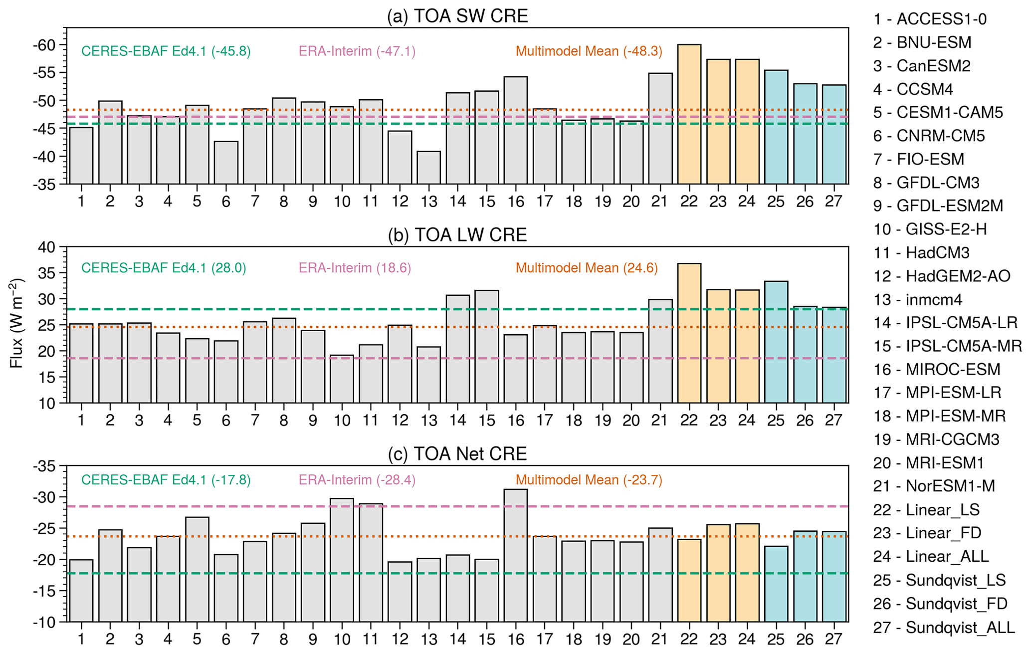
Figure 17Globally averaged TOA (a) shortwave (SW), (b) longwave (LW) and (c) net cloud radiative effects (CREs, W m−2) from 21 CMIP5 models historical runs (1996–2005, gray bars) and Isca simulations with different setups (orange bars for linear scheme and cyan bars for Sundqvist scheme). The horizontal lines are annual and global mean CREs from CERES-EBAF (dashed green lines, covering from 2001 to 2018) and the multimodel ensemble mean results (dotted orange lines) of CMIP5 models, whose names are listed on the right for reference.
We can also use a Taylor diagram (Taylor, 2001) to compare Isca with other models, as this summarizes the standard deviation, pattern correlation and root-mean-square error (RMSE) in a single plot. Figure 18 shows the statistics of the observed and simulated LW, SW and net CREs from CMIP5 historical simulations (1996–2005) and Isca simulations. Compared to CMIP5 models, the LS runs from both the linear and Sundqvist schemes display large RMSEs and low spatial correlations for the LW CRE field (Fig. 18a), likely a consequence of too much cloud in polar regions. Similarly, the net CREs in the LS runs also show larger RMSEs and standard deviations than most CMIP5 models (Fig. 18c). The FD and ALL simulations improve matters: going from the LS to FD simulations the RMSE decreases from 12.1 to 9.0 W m−2 and from 18.6 to 14.5 W m−2 for LW and net CREs, respectively. For the SW CREs (Fig. 18b), compared to the LS runs, the RMSEs in the ALL runs have decreased slightly in both linear and Sundqvist schemes. By these metrics, the simple cloud scheme is performing similarly to a number of CMIP5 models.

Figure 18Taylor diagrams showing standard deviation (W m−2), root-mean-square error (RMSE; W m−2) and spatial pattern correlation for the observed and simulated (a) LW, (b) SW and (c) net CREs at TOA in CMIP5 models and Isca simulations (LS, FD and ALL). The statistics of these variables are calculated based on annual mean data, where the monthly data (1996–2005) from historical simulation are used for analysis of CMIP5 models. The observed field is as a reference and denoted by a black star. Contour of the standard deviation from the observed field is shown by the dashed black line, and the contours of the RMSE are displayed in gray with labels.
4.5 Parameter sensitivity of the scheme
Thus far we have largely selected the various parameter values using observations. In order to test the sensitivity to these choices, a small number of simulations with different parameters are conducted. The simulations analyzed here are run for 10 years, and the last 5 years are used for analysis.
The parameters used in the simulation are the default values introduced previously; i.e., the effective radii for liquid and ice clouds particles are re_liq=14 and re_ice=25 µm, respectively, and the maximum in-cloud liquid water content that one grid box can reach is wl0=0.18 g kg−1. As displayed in Table 4, changing the value of the effective radius for liquid clouds has little impact on LW flux and CRE at TOA but has a large impact on those fields associated with the SW flux. For instance, the net SW flux at TOA has reduced (increased) by about 4.1 W m−2 (9.7 W m−2) when the effective radius of liquid cloud decreases (increases) from 14 to 12 µm (16 µm), which can be explained by the relationship between effective radius (re) and shortwave optical depth (τ) of clouds, , where LWP is the liquid water path (g m−2) of clouds and re is in micrometers (µm) (Stephens, 1978). Specifically, if the liquid water path remains unchanged, then τ increases (decreases) with the decrease (increase) in re (e.g., Slingo and Schrecker, 1982), implying that the reflected SW flux would increase (decrease), the net SW flux at TOA would decrease (increase) and the SW CRE would get more (less) negative.
Table 4Global and annual mean climatology from parameter sensitivity tests. In each test, only the parameter listed in the table header (see Table 1) is changed from the default values. The units for cloud effective radius (re) and in-cloud liquid water mixing ratio (wl) are μm and g kg−1, respectively.
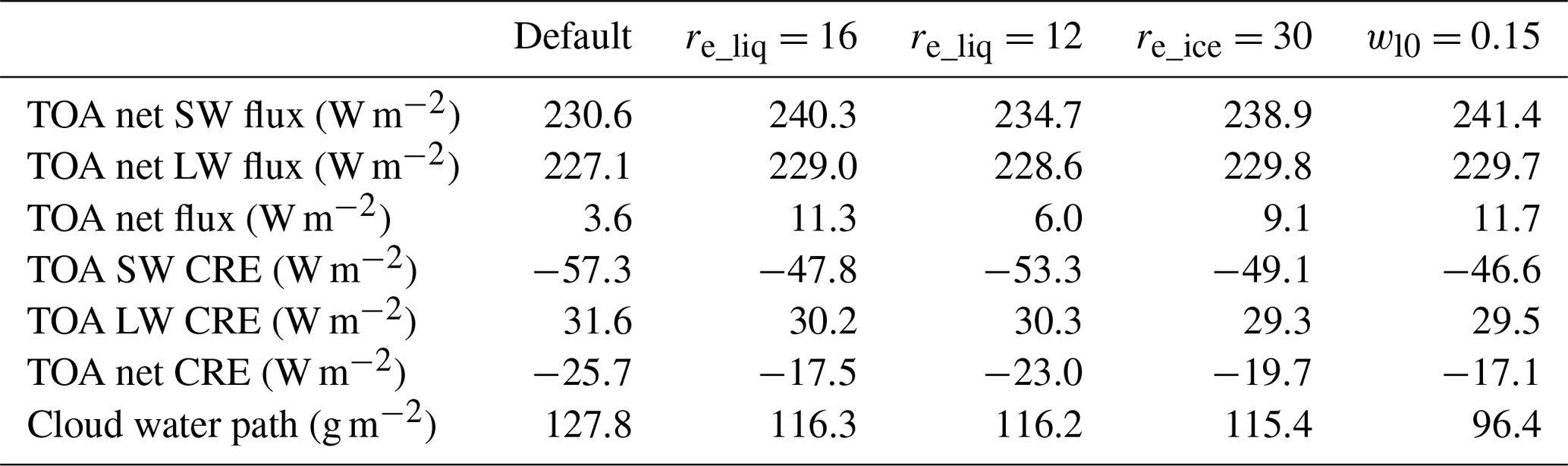
As introduced in Sect. 2, ice clouds are treated as liquid clouds, except that the effective radius is different. Thus the increase in effective radius of ice clouds has similar effect of the increase in effective radius of liquid clouds, resulting in the increase in net SW flux and less negative SW CRE at the TOA (see the fourth column in Table 4). However, what is different is that tuning the effective radius of ice clouds can also influence the LW related flux and CRE, as the ice clouds are usually located at high levels.
In addition, when decreasing the maximum value of in-cloud water mixing ratio that a grid box can reach (i.e., wl0) from 0.18 to 0.15 g kg−1, the global mean LWP decreases over 30 g m−2 (last column in Table 4). In this case, if the re is unchanged, then τ would decrease in response to the decrease in LWP. Hence, the atmosphere becomes less opaque, which has an opposite effect of reducing re and thus the net SW flux at TOA increases and the SW CRE becomes less negative. Therefore, these parameters can be used to adjust the radiative properties associated with SW. We note that tuning wl can also impact LW radiative fluxes.
As mentioned in Sect. 2, the coefficient a in the linear scheme is related to the critical relative humidity. Therefore, the parameter as in Eq. (2), which is related to the critical relative humidity at lower levels, can be used to tune the SW CRE. Changing the parameter at in Eq. (2), which determines the coefficient profile (and the critical relative humidity) at high levels, impacts both the LW and SW CRE (the results not shown here). In general, all the parameters associated with the critical relative humidity (as or at), effective radius and cloud liquid water content can be used to tune the SW and LW CREs, and users can determine which one to use based on their research purpose.
We have presented and explored a simple diagnostic cloud scheme, SimCloud, with two general aims. First, we hope to provide a scheme whose dependence on various parameters and processes is transparent, so it can be used to explore and understand the cloud distribution and its possible changes in the future, as well as possible differences among models. Second, we hope to provide a cloud scheme at a modest level of complexity that can be used in GCMs in a broad range of situations where some basic representation of cloud cover would be useful. For example, prior to the implementation of SimCloud, Isca did not have a cloud scheme. By adding SimCloud to Isca, we have improved the simulated radiative properties.
This simple diagnostic scheme is not meant as a replacement for more complicated schemes that are based on microphysical properties and/or explicitly on liquid and solid phases of the condensate. Rather, it is intended to be used in models that may require a level of complexity commensurate with other parameterizations and/or in situations where particular processes are to be investigated. Cloud schemes in many comprehensive GCMs have become very complicated and differ considerably in detail from each other, and we think there is value in providing a simpler scheme that also has a number of realistic features and that captures the observed cloud climatology with some verisimilitude.
The cloud fraction, the effective radius of the cloud droplet and in-cloud water mixing ratio are parameterized in SimCloud. The cloud fraction parameterization includes two kinds of clouds: large-scale clouds and marine low clouds, with the addition of a “freeze-dry” adjustment. The effective radius of cloud droplets is calculated as a weighted mean of liquid cloud droplet and ice cloud crystal, with the weight specified by the liquid cloud fraction, which is defined as a linear function of temperature. The in-cloud liquid water content is also determined as a function of temperature, where the temperature threshold is deduced from the observed liquid and ice cloud top temperature. The equations and parameters used in this cloud scheme are summarized in Table 1. The parameters themselves are user-configurable; here we merely present those that we have found to be useful.
The large-scale clouds are diagnosed from relative humidity and there are two options for the scheme: the first is a linear relationship of relative humidity, where the coefficient profile is derived from hourly reanalysis data sets; the second one has the same form as the Sundqvist scheme. The code is quite flexible and other choices could readily be implemented. Simulations with large-scale clouds only (LS simulation) show that this method does capture the basic features of spatial patterns of cloud fraction and CREs at TOA. Using the linear relation connecting cloud fraction to relative humidity gives similar results to those from the Sundqvist scheme (which uses a square-root dependency). However, both relative humidity schemes were found to have two deficiencies. The first is that the cloud cover is generally too high in the high latitudes, especially over polar regions, which in turn leads to an overestimated CRE over these regions. These biases can not only be found in annual mean spatial patterns but also in the seasonal cycles. The second issue is the underestimation of cloud fractions, and hence the SW and net CREs, in the marine stratocumulus regions off the west coast of continents; this has also been a long-standing problem in CMIP3 and CMIP5 models (Dolinar et al., 2015).
In order to mitigate the biases of extra clouds over polar regions, a modified freeze-dry method from Vavrus and Waliser (2008) may be used, in which the cloud fractions over high latitudes are adjusted by a function of specific humidity. With this method, the seasonal cycle of cloud fraction over the Arctic was found to be well simulated and the cloud fraction was found to be more realistic, especially in winter. The improvement of the cloud fraction over high latitudes also decreases the CRE biases, contributing to the improvement of the seasonal cycle of LW CREs. We should note that in this adjustment the specific humidity thresholds are derived according to current climate, but whether the threshold holds under global warming still needs further investigation. To alleviate the problem of the low-cloud biases, a diagnostic low-cloud scheme based on the estimated low-level cloud fraction (ELF) from Park and Shin (2019) was implemented, as the ELF shows a good linear relationship with low-cloud fraction in the reanalysis data set. The simulation with both large-scale clouds and low clouds (the ALL simulation) reduced the SW and net CRE biases off the west continental regions over subtropics by increasing both the cloud fraction and the cloud water path.
In summary, many of the basic features of observed cloud fraction and cloud radiative properties are captured by the cloud scheme. Using SimCloud, Isca is able to reasonably reproduce the observed spatial and temporal variability of clouds, comparable to a number of CMIP5 models that use more complicated schemes. This suggests that SimCloud might be suitable to study problems related to cloud feedback and cloud–circulation coupling. In addition, the scheme is relative flexible and many aspects are optional or user-configurable, so the users can decide which one to use as per their own research interests or purposes. For example, if the users do not focus on the polar regions, they can omit the freeze-dry adjustment.
Certainly, the scheme has deficiencies. For example, the SW CREs are still a little weak off the west coast of continents and too strong over the extratropics compared to observations. The global mean CREs, including the LW and SW CREs, are too strong, and the TOA radiation imbalance is rather large compared to the observations, which perhaps could be solved by further improvements of the cloud scheme, e.g., including the microphysical processes. It should be noted that in addition to the cloud scheme, other physical processes such as precipitation are also important components in GCMs, and the improvements in these processes can also help to reduce GCM biases. For example, the incorporation of prognostic precipitation scheme in MIROC6-SPRINTARS model (Michibata et al., 2019) has improved some systematic biases in both the magnitude of aerosol–cloud interactions and in rain formation processes with more realistic cloud and radiation fields, indicating that the process-based model development is also important to help us better understand the climate system.
Finally, at a more general level, the diagnostic scheme we have presented does not vary with model resolution and thus is not “scale aware”. Whereas this may be perfectly appropriate at low and modest resolutions, it would fail as the model resolution increases because the distribution of relative humidity varies according to the resolution, and thus the functional dependence of cloud fraction should be a function of grid size. This drawback is not, however, unique to our scheme. It could be overcome at an empirical level by retuning the coefficients as resolution changes. We have not found this to be an issue in practice at the resolutions we have used. If desired, it may be possible to address this using a more sophisticated treatment of the distribution properties of humidity, with the width of the moisture distribution (and hence the critical value of relative humidity) then becoming a function of grid size and/or being dynamically determined. Separate schemes to take into account the low-level inversion and polar effects would then ideally not be needed. It would also be of interest to further simplify the scheme so that it could, for example, be coupled to simpler (e.g., semi-gray) radiation schemes with less complicated treatments of scattering and absorption and which might be more appropriate for very different climate regimes. These are topics for future work.
The SimCloud code can be accessed at https://doi.org/10.5281/zenodo.4382536 (Liu et al., 2020) under the GNU General Public License v3.0, and the updates can be found at https://github.com/lqxyz/Isca/tree/simple_clouds (last access: 1 May 2021). It will be merged with the Isca (Vallis et al., 2018) master repository on Github in the future. Please refer to the Supplement for a brief introduction to the code structure. The Isca model outputs produced for this study are available on Zenodo: https://doi.org/10.5281/zenodo.4573610 (Liu et al., 2021). An archive of the scripts used to process data and generate the figures and tables is available at https://doi.org/10.5281/zenodo.4597263 (Liu, 2021), and the updates can be found at https://github.com/lqxyz/cloud_scheme_manuscript_figs (last access: 1 May 2021).
The supplement related to this article is available online at: https://doi.org/10.5194/gmd-14-2801-2021-supplement.
QL implemented the cloud scheme, performed the simulations and analyzed the results under the supervision of MC and GKV. PM and SIT implemented an early revision of the cloud scheme and provided technical support. All authors contributed to the results analysis and the editing of the manuscript.
The authors declare that they have no conflict of interest.
We thank the editor and two anonymous reviewers for their helpful comments. We gratefully thank Paulo Ceppi, Mark Webb and other members of the phase II of SPOOKIE project for providing the in-cloud liquid water mixing ratio formula in Eq. (12). We thank Greg Colyer and Ruth Geen for providing the filtered land topography file used in the simulations. We also thank Yannick Copin for sharing the script for Taylor diagram (https://gist.github.com/ycopin/3342888#file-taylordiagram-py, last access: 1 May 2021). We acknowledge the groups for making the following data sets public available: input4MIPs (https://esgf-node.llnl.gov/projects/input4mips, last access: 1 May 2021), ERA-Interim (https://www.ecmwf.int/en/forecasts/datasets/archive-datasets/reanalysis-datasets/era-interim, last access: 1 May 2021), ERA5 (https://cds.climate.copernicus.eu/cdsapp#!/home, last access: 1 May 2021), CALIPSO-GOCCP (https://climserv.ipsl.polytechnique.fr/cfmip-obs/Calipso_goccp.html, last access: 1 May 2021), CloudSat (http://www.cloudsat.cira.colostate.edu/data-products/level-2b/2b-cwc-ro, last access: 1 May 2021) and CERES-EBAF (https://ceres.larc.nasa.gov/compare_products.php, last access: 1 May 2021). We also thank the Centre for Environmental Data Analysis (https://www.ceda.ac.uk, last access: 1 May 2021) for making the CMIP5 outputs available. Qun Liu is supported by the joint scholarship from University of Exeter and China Scholarship Council (no. 201706210070). Matthew Collins acknowledges support from the Natural Environment Research Council (NERC, grant no. NE/N018486/1). Penelope Maher is supported by the NERC (grant no. NE/T003863/1), and Stephen I. Thomson is supported by the UK-China Research and Innovation Partnership Fund, through the Met Office Climate Science for Service Partnership (CSSP) China, as part of the Newton Fund. Geoffrey K. Vallis and Matthew Collins are also supported by the NERC (grant no. NE/T006285/1: “Circulation, Clouds and Climate Sensitivity”).
This research has been supported by the Natural Environment Research Council (grant nos. NE/N018486/1, NE/T003863/1, and NE/T006285/1), the China Scholarship Council (grant no. 201706210070), and UK-China Research and Innovation Partnership Fund, through the Met Office Climate Science for Service Partnership (CSSP) China as part of the Newton Fund.
This paper was edited by Sylwester Arabas and reviewed by two anonymous referees.
Austin, R. T., Heymsfield, A. J., and Stephens, G. L.: Retrieval of ice cloud microphysical parameters using the CloudSat millimeter-wave radar and temperature, J. Geophys. Res., 114, D00A23, https://doi.org/10.1029/2008jd010049, 2009. a
Bodas-Salcedo, A., Webb, M., Bony, S., Chepfer, H., Dufresne, J.-L., Klein, S., Zhang, Y., Marchand, R., Haynes, J., Pincus, R., and John, V.: COSP: Satellite simulation software for model assessment, B. Am. Meteorol. Soc., 92, 1023–1043, https://doi.org/10.1175/2011bams2856.1, 2011. a
Bony, S. and Dufresne, J.-L.: Marine boundary layer clouds at the heart of tropical cloud feedback uncertainties in climate models, Geophys. Res. Lett., 32, L20806, https://doi.org/10.1029/2005gl023851, 2005. a
Bony, S., Dufresne, J.-L., Le Treut, H., Morcrette, J.-J., and Senior, C.: On dynamic and thermodynamic components of cloud changes, Clim. Dynam., 22, 71–86, https://doi.org/10.1007/s00382-003-0369-6, 2004. a, b
Boville, B. A., Rasch, P. J., Hack, J. J., and McCaa, J. R.: Representation of clouds and precipitation processes in the Community Atmosphere Model version 3 (CAM3), J. Climate, 19, 2184–2198, https://doi.org/10.1175/jcli3749.1, 2006. a, b, c
Ceppi, P., Brient, F., Zelinka, M. D., and Hartmann, D. L.: Cloud feedback mechanisms and their representation in global climate models, WIREs Clim. Change, 8, e465, https://doi.org/10.1002/wcc.465, 2017. a
Chepfer, H., Bony, S., Winker, D., Cesana, G., Dufresne, J., Minnis, P., Stubenrauch, C., and Zeng, S.: The GCM-oriented CALIPSO cloud product (CALIPSO-GOCCP), J. Geophys. Res., 115, D00H16, https://doi.org/10.1029/2009jd012251, 2010. a
Collins, W. D., Rasch, P. J., Boville, B. A., Hack, J. J., McCaa, J. R., Williamson, D. L., Kiehl, J. T., Briegleb, B., Bitz, C., and Lin, S.-J., Zhang, M., and Dai, Y.: Description of the NCAR community atmosphere model (CAM 3.0), NCAR, Tech. Note NCAR/TN-464+ STR, Vol. 226, https://doi.org/10.5065/D63N21CH, 2004. a, b, c, d
Copernicus Climate Change Service (C3S) (2017): ERA5: Fifth generation of ECMWF atmospheric reanalyses of the global climate,, Copernicus Climate Change Service Climate Data Store (CDS), available at: https://cds.climate.copernicus.eu/cdsapp#!/home (last access: 12 July 2020), 2017. a
Dee, D., Uppala, S., Simmons, A., Berrisford, P., Poli, P., Kobayashi, S., Andrae, U., Balmaseda, M., Balsamo, G., Bauer, P., Bechtold, P., Beljaars, A., van de Berg, L., Bidlot, J., Bormann, N., Delsol, C., Dragani, R., Fuentes, M., Geer, A., Haimberger, L., Healy, S., Hersbach, H., Hólm, E., Isaksen, L., Kållberg, P., Köhler, M., Matricardi, M., McNally, A., Monge-Sanz, B., Morcrette, J.-J., Park, B.-K., Peubey, C., de Rosnay, P., Tavolato, C., Thépaut, J.-N., and Vitart, F.: The ERA-Interim reanalysis: Configuration and performance of the data assimilation system, Q. J. Roy. Meteor. Soc., 137, 553–597, https://doi.org/10.1002/qj.828, 2011. a, b
Dolinar, E. K., Dong, X., Xi, B., Jiang, J. H., and Su, H.: Evaluation of CMIP5 simulated clouds and TOA radiation budgets using NASA satellite observations, Clim. Dynam., 44, 2229–2247, https://doi.org/10.1007/s00382-014-2158-9, 2015. a, b, c, d
Durack, P., Taylor, K., Eyring, V., Ames, S., Hoang, T., Nadeau, D., Doutriaux, C., Stockhause, M., and Gleckler, P.: Toward standardized data sets for climate model experimentation, Eos, 99, https://doi.org/10.1029/2018EO101751, 2018. a
Edwards, J. and Slingo, A.: Studies with a flexible new radiation code. I: Choosing a configuration for a large-scale model, Q. J. Roy. Meteor. Soc., 122, 689–719, https://doi.org/10.1002/qj.49712253107, 1996. a
Frierson, D. M.: The dynamics of idealized convection schemes and their effect on the zonally averaged tropical circulation, J. Atmos. Sci., 64, 1959–1976, https://doi.org/10.1175/jas3935.1, 2007. a, b, c
Frierson, D. M., Held, I. M., and Zurita-Gotor, P.: A gray-radiation aquaplanet moist GCM. Part I: Static stability and eddy scale, J. Atmos. Sci., 63, 2548–2566, https://doi.org/10.1175/jas3753.1, 2006. a
Giorgetta, M., Brokopf, R., Crueger, T., Esch, M., Fiedler, S., Helmert, J., Hohenegger, C., Kornblueh, L., Köhler, M., Manzini, E., Mauritsen, T., Nam, C., Raddatz, T., Rast, S., Reinert, D., Sakradzija, M., Schmidt, H., Schneck, R., Schnur, R., Silvers, L., Wan, H., Zängl, G., and Stevens, B.: ICON-A, the atmosphere component of the ICON Earth System Model: I. Model description, J. Adv. Model. Earth Sy., 10, 1613–1637, https://doi.org/10.1029/2017ms001242, 2018. a
Gordon, C.: Comparison of 30-day integrations with and without cloud-radiation interaction, Mon. Weather Rev., 120, 1244–1278, https://doi.org/10.1175/1520-0493(1992)120<1244:codiwa>2.0.co;2, 1992. a
Guo, Z. and Zhou, T.: An improved diagnostic stratocumulus scheme based on estimated inversion strength and its performance in GAMIL2, Sci. China Earth Sci., 57, 2637–2649, https://doi.org/10.1007/s11430-014-4891-7, 2014. a
Hartmann, D. L.: Global Physical Climatology, 2nd edn., Elsevier, Boston, 485 pp., https://doi.org/10.1016/C2009-0-00030-0, 2016. a
Hartmann, D. L., Ockert-Bell, M. E., and Michelsen, M. L.: The effect of cloud type on Earth's energy balance: Global analysis, J. Climate, 5, 1281–1304, https://doi.org/10.1175/1520-0442(1992)005<1281:teocto>2.0.co;2, 1992. a
Heymsfield, A. J. and Miloshevich, L. M.: Homogeneous ice nucleation and supercooled liquid water in orographic wave clouds, J. Atmos. Sci., 50, 2335–2353, https://doi.org/10.1175/1520-0469(1993)050<2335:hinasl>2.0.co;2, 1993. a
Holloway, J. L. and Manabe, S.: Simulation of climate by a global general circulation model, Mon. Weather Rev., 99, 335–370, https://doi.org/10.1175/1520-0493(1971)099<0335:socbag>2.3.co;2, 1971. a
Houze, R. A.: Cloud dynamics, 2nd edn., Academic Press, San Diego, Vol. 104, 432 pp., ISBN 978-0-12-374266-7, 2014. a
Jones, C. G., Wyser, K., Ullerstig, A., and Willén, U.: The Rossby Centre Regional Atmospheric Climate Model Part II: Application to the Arctic climate, AMBIO, 33, 211–220, https://doi.org/10.1579/0044-7447-33.4.211, 2004. a
Joshi, M., Stringer, M., van der Wiel, K., O'Callaghan, A., and Fueglistaler, S.: IGCM4: a fast, parallel and flexible intermediate climate model, Geosci. Model Dev., 8, 1157–1167, https://doi.org/10.5194/gmd-8-1157-2015, 2015. a
Kawai, H. and Inoue, T.: A simple parameterization scheme for subtropical marine stratocumulus, SOLA, 2, 17–20, https://doi.org/10.2151/sola.2006-005, 2006. a
Kawai, H., Koshiro, T., and Webb, M. J.: Interpretation of factors controlling low cloud cover and low cloud feedback using a unified predictive index, J. Climate, 30, 9119–9131, https://doi.org/10.1175/jcli-d-16-0825.1, 2017. a
Kawai, H., Yukimoto, S., Koshiro, T., Oshima, N., Tanaka, T., Yoshimura, H., and Nagasawa, R.: Significant improvement of cloud representation in the global climate model MRI-ESM2, Geosci. Model Dev., 12, 2875–2897, https://doi.org/10.5194/gmd-12-2875-2019, 2019. a, b
Klein, S. A. and Hartmann, D. L.: The seasonal cycle of low stratiform clouds, J. Climate, 6, 1587–1606, https://doi.org/10.1175/1520-0442(1993)006<1587:tscols>2.0.co;2, 1993. a, b, c
Lauer, A. and Hamilton, K.: Simulating clouds with global climate models: A comparison of CMIP5 results with CMIP3 and satellite data, J. Climate, 26, 3823–3845, https://doi.org/10.1175/jcli-d-12-00451.1, 2013. a
Lenaerts, J. T., Van Tricht, K., Lhermitte, S., and L'Ecuyer, T. S.: Polar clouds and radiation in satellite observations, reanalyses, and climate models, Geophys. Res. Lett., 44, 3355–3364, https://doi.org/10.1002/2016gl072242, 2017. a
Li, J., Mao, J., and Wang, F.: Comparative study of five current reanalyses in characterizing total cloud fraction and top-of-the-atmosphere cloud radiative effects over the Asian monsoon region, Int. J. Climatol., 37, 5047–5067, https://doi.org/10.1002/joc.5143, 2017. a, b
Liu, Q.: Cloud scheme manuscript figures (Version v2), Zenodo [data set], https://doi.org/10.5281/zenodo.4597263, 2021 (updates available at: https://github.com/lqxyz/cloud_scheme_manuscript_figs, last access: 1 May 2021). a
Liu, Q., Collins, M., Maher, P., Thomson, S. I., and Vallis, G. K.: SimCloud version 1.0 incorporated in Isca framework (Version v1.0rc), Zenodo [code], https://doi.org/10.5281/zenodo.4382536, 2020 (updates available at: https://github.com/lqxyz/Isca/tree/simple_clouds, last access: 1 May 2021). a
Liu, Q., Collins, M., Maher, P., Thomson, S. I., and Vallis, G. K.: Outputs from Isca simulations with simple cloud scheme and SOCRATES radiation scheme, Zenodo [data set], https://doi.org/10.5281/zenodo.4573610, 2021. a
Loeb, N. G., Wielicki, B. A., Doelling, D. R., Smith, G. L., Keyes, D. F., Kato, S., Manalo-Smith, N., and Wong, T.: Toward optimal closure of the Earth's top-of-atmosphere radiation budget, J. Climate, 22, 748–766, https://doi.org/10.1175/2008jcli2637.1, 2009. a
Loeb, N. G., Doelling, D. R., Wang, H., Su, W., Nguyen, C., Corbett, J. G., Liang, L., Mitrescu, C., Rose, F. G., and Kato, S.: Clouds and the Earth's radiant energy system (CERES) energy balanced and filled (EBAF) top-of-atmosphere (TOA) edition-4.0 data product, J. Climate, 31, 895–918, https://doi.org/10.1175/jcli-d-17-0208.1, 2018. a
Maher, P., Vallis, G. K., Sherwood, S. C., Webb, M. J., and Sansom, P. G.: The impact of parameterized convection on climatological precipitation in atmospheric global climate models, Geophys. Res. Lett., 45, 3728–3736, https://doi.org/10.1002/2017gl076826, 2018. a
Maher, P., Gerber, E. P., Medeiros, B., Merlis, T. M., Sherwood, S., Sheshadri, A., Sobel, A. H., Vallis, G. K., Voigt, A., and Zurita‐Gotor, P.: Model hierarchies for understanding atmospheric circulation, Rev. Geophys., 57, 250–280, https://doi.org/10.1029/2018rg000607, 2019. a
Manners, J., Edwards, J. M., Hill, P., and Thelen, J.-C.: SOCRATES (Suite Of Community RAdiative Transfer codes based on Edwards and Slingo) Technical Guide, Met Office, UK, 2015. a
Michibata, T., Suzuki, K., Sekiguchi, M., and Takemura, T.: Prognostic precipitation in the MIROC6-SPRINTARS GCM: description and evaluation against satellite observations, J. Adv. Model. Earth Sy., 11, 839–860, https://doi.org/10.1029/2018MS001596, 2019. a
Ming, Y. and Held, I. M.: Modeling water vapor and clouds as passive tracers in an idealized GCM, J. Climate, 31, 775–786, https://doi.org/10.1175/jcli-d-16-0812.1, 2018. a
Morcrette, J.-J. and Jakob, C.: The response of the ECMWF model to changes in the cloud overlap assumption, Mon. Weather Rev., 128, 1707–1732, https://doi.org/10.1175/1520-0493(2000)128<1707:trotem>2.0.co;2, 2000. a
Nam, C., Bony, S., Dufresne, J.-L., and Chepfer, H.: The “too few, too bright” tropical low-cloud problem in CMIP5 models, Geophys. Res. Lett., 39, L21801, https://doi.org/10.1029/2012gl053421, 2012. a, b
Ose, T.: An examination of the effects of explicit cloud water in the UCLA GCM, J. Meteorol. Soc. Jpn., 71, 93–109, https://doi.org/10.2151/jmsj1965.71.1_93, 1993. a, b, c
Park, S. and Shin, J.: Heuristic estimation of low-level cloud fraction over the globe based on a decoupling parameterization, Atmos. Chem. Phys., 19, 5635–5660, https://doi.org/10.5194/acp-19-5635-2019, 2019. a, b, c, d
Park, S., Bretherton, C. S., and Rasch, P. J.: Integrating cloud processes in the Community Atmosphere Model, version 5, J. Climate, 27, 6821–6856, https://doi.org/10.1175/jcli-d-14-00087.1, 2014. a
Qin, Y., Lin, Y., Xu, S., Ma, H., and Xie, S.: A diagnostic PDF cloud scheme to improve subtropical low clouds in NCAR Community Atmosphere Model (CAM 5), J. Adv. Model. Earth Sy., 10, 320–341, https://doi.org/10.1002/2017ms001095, 2018. a
Qu, X., Hall, A., Klein, S. A., and Caldwell, P. M.: On the spread of changes in marine low cloud cover in climate model simulations of the 21st century, Clim. Dynam., 42, 2603–2626, https://doi.org/10.1007/s00382-013-1945-z, 2014. a
Quaas, J.: Evaluating the “critical relative humidity” as a measure of subgrid-scale variability of humidity in general circulation model cloud cover parameterizations using satellite data, J. Geophys. Res., 117, D09208, https://doi.org/10.1029/2012jd017495, 2012. a, b, c
Ramanathan, V., Cess, R., Harrison, E., Minnis, P., Barkstrom, B., Ahmad, E., and Hartmann, D.: Cloud-radiative forcing and climate: Results from the Earth Radiation Budget Experiment, Science, 243, 57–63, https://doi.org/10.1126/science.243.4887.57, 1989. a, b, c
Ricketts, J.: An investigation into a relationship between upper-air relative humidity and cloud cover, Meteorol. Mag., 102, 146–153, 1973. a
Roehrig, R., Beau, I., Saint‐Martin, D., Alias, A., Decharme, B., Guérémy, J., Voldoire, A., Abdel‐Lathif, A. Y., Bazile, E., Belamari, S., Blein, S., Bouniol, D., Bouteloup, Y., Cattiaux, J., Chauvin, F., Chevallier, M., Colin, J., Douville, H., Marquet, P., Michou, M., Nabat, P., Oudar, T., Peyrillé, P., Piriou, J., Salas y Mélia, D., Séférian, R., and Sénési, S.: The CNRM global atmosphere model ARPEGE-Climat 6.3: description and evaluation, J. Adv. Model. Earth Sy., 12, e2020MS002075, https://doi.org/10.1029/2020ms002075, 2020. a
Ryan, B.: On the global variation of precipitating layer clouds, B. Am. Meteorol. Soc., 77, 53–70, https://doi.org/10.1175/1520-0477(1996)077<0053:otgvop>2.0.co;2, 1996. a
Slingo, A.: Sensitivity of the Earth's radiation budget to changes in low clouds, Nature, 343, 49–51, https://doi.org/10.1038/343049a0, 1990. a
Slingo, A. and Schrecker, H.: On the shortwave radiative properties of stratiform water clouds, Q. J. Roy. Meteor. Soc., 108, 407–426, https://doi.org/10.1002/qj.49710845607, 1982. a
Slingo, J.: The development and verification of a cloud prediction scheme for the ECMWF model, Q. J. Roy. Meteor. Soc., 113, 899–927, https://doi.org/10.1002/qj.49711347710, 1987. a, b, c
Slingo, J. M.: A cloud parametrization scheme derived from GATE data for use with a numerical model, Q. J. Roy. Meteor. Soc., 106, 747–770, https://doi.org/10.1002/qj.49710645008, 1980. a
Smagorinsky, J.: On the dynamical prediction of large-scale condensation by numerical methods, in: Geophysical Monograph Series, edited by: Weickmann, H., American Geophysical Union, 5, 71–78, https://doi.org/10.1029/gm005p0071, 1960. a
Smith, R.: A scheme for predicting layer clouds and their water content in a general circulation model, Q. J. Roy. Meteor. Soc., 116, 435–460, https://doi.org/10.1002/qj.49711649210, 1990. a, b, c
Sommeria, G. and Deardorff, J.: Subgrid-scale condensation in models of nonprecipitating clouds, J. Atmos. Sci., 34, 344–355, https://doi.org/10.1175/1520-0469(1977)034<0344:sscimo>2.0.co;2, 1977. a, b
Stensrud, D. J.: Parameterization schemes, Cambridge University Press, Cambridge, https://doi.org/10.1017/cbo9780511812590, 2007. a
Stephens, G. L.: Radiation profiles in extended water clouds. II: Parameterization schemes, J. Atmos. Sci., 35, 2123–2132, https://doi.org/10.1175/1520-0469(1978)035<2123:RPIEWC>2.0.CO;2, 1978. a
Stocker, T. F., Qin, D., Plattner, G.-K., Tignor, M., Allen, S. K., Boschung, J., Nauels, A., Xia, Y., Bex, V., and Midgley, P. M. (Eds.): Climate Change 2013 – The Physical Science Basis: Working Group I Contribution to the Fifth Assessment Report of the Intergovernmental Panel on Climate Change, Cambridge University Press, Cambridge, 1535 pp., ISBN 9781107415324, 2013. a
Stubenrauch, C., Rossow, W., Kinne, S., Ackerman, S., Cesana, G., Chepfer, H., Di Girolamo, L., Getzewich, B., Guignard, A., Heidinger, A., Maddux, B., Menzel, W., Minnis, P., Pearl, C., Platnick, S., Poulsen, C., Riedi, J., Sun-Mack, S., Walther, A., Winker, D., Zeng, S., and Zhao, G.: Assessment of global cloud datasets from satellites: Project and database initiated by the GEWEX radiation panel, B. Am. Meteorol. Soc., 94, 1031–1049, https://doi.org/10.1175/bams-d-12-00117.1, 2013. a, b, c
Sundqvist, H., Berge, E., and Kristjánsson, J. E.: Condensation and cloud parameterization studies with a mesoscale numerical weather prediction model, Mon. Weather Rev., 117, 1641–1657, https://doi.org/10.1175/1520-0493(1989)117<1641:cacpsw>2.0.co;2, 1989. a, b, c, d, e, f
Taylor, K. E., Williamson, D., and Zwiers, F.: The Sea surface Temperature and sea-ice concentration boundary concentrations for AMIP II simulations, PMCDI Rep. No. 60, available at: https://pcmdi.llnl.gov/report/pdf/60.pdf (last acess: 1 May 2021), 2000. a
Taylor, K. E.: Summarizing multiple aspects of model performance in a single diagram, J. Geophys. Res., 106, 7183–7192, https://doi.org/10.1029/2000jd900719, 2001. a
Thomson, S. I. and Vallis, G. K.: Atmospheric response to SST anomalies. Part I: Background-state dependence, teleconnections, and local effects in winter, J. Atmos. Sci., 75, 4107–4124, https://doi.org/10.1175/jas-d-17-0297.1, 2018. a
Thomson, S. I. and Vallis, G. K.: Hierarchical modeling of solar system planets with Isca, Atmosphere-Basel, 10, 803, https://doi.org/10.3390/atmos10120803, 2019. a, b
Tiedtke, M.: Representation of clouds in large-scale models, Mon. Weather Rev., 121, 3040–3061, https://doi.org/10.1175/1520-0493(1993)121<3040:rocils>2.0.co;2, 1993. a
Tompkins, A. M.: A prognostic parameterization for the subgrid-scale variability of water vapor and clouds in large-scale models and its use to diagnose cloud cover, J. Atmos. Sci., 59, 1917–1942, https://doi.org/10.1175/1520-0469(2002)059<1917:appfts>2.0.co;2, 2002. a
Tompkins, A. M.: The parametrization of cloud cover, ECMWF Moist Processes Lecture Note Series, 25, 23 pp., available at: https://www.ecmwf.int/node/16958 (last acess: 1 May 2021), 2005. a, b
Tsang, Y.-K. and Vallis, G. K.: A stochastic Lagrangian basis for a probabilistic parameterization of moisture condensation in Eulerian models, J. Atmos. Sci., 75, 3925–3941, https://doi.org/10.1175/jas-d-18-0065.1, 2018. a, b
Vallis, G. K., Colyer, G., Geen, R., Gerber, E., Jucker, M., Maher, P., Paterson, A., Pietschnig, M., Penn, J., and Thomson, S. I.: Isca, v1.0: a framework for the global modelling of the atmospheres of Earth and other planets at varying levels of complexity, Geosci. Model Dev., 11, 843–859, https://doi.org/10.5194/gmd-11-843-2018, 2018. a, b, c
Vavrus, S. and Waliser, D.: An improved parameterization for simulating Arctic cloud amount in the CCSM3 climate model, J. Climate, 21, 5673–5687, https://doi.org/10.1175/2008jcli2299.1, 2008. a, b, c, d, e
Walters, D., Baran, A. J., Boutle, I., Brooks, M., Earnshaw, P., Edwards, J., Furtado, K., Hill, P., Lock, A., Manners, J., Morcrette, C., Mulcahy, J., Sanchez, C., Smith, C., Stratton, R., Tennant, W., Tomassini, L., Van Weverberg, K., Vosper, S., Willett, M., Browse, J., Bushell, A., Carslaw, K., Dalvi, M., Essery, R., Gedney, N., Hardiman, S., Johnson, B., Johnson, C., Jones, A., Jones, C., Mann, G., Milton, S., Rumbold, H., Sellar, A., Ujiie, M., Whitall, M., Williams, K., and Zerroukat, M.: The Met Office Unified Model Global Atmosphere 7.0/7.1 and JULES Global Land 7.0 configurations, Geosci. Model Dev., 12, 1909–1963, https://doi.org/10.5194/gmd-12-1909-2019, 2019. a
Webb, M. J., Lock, A. P., Bretherton, C. S., Bony, S., Cole, J. N., Idelkadi, A., Kang, S. M., Koshiro, T., Kawai, H., Ogura, T., Roehrig, R., Shin, Y., Mauritsen, T., Sherwood, S. C., Vial, J., Watanabe, M., Woelfle, M. D., and Zhao, M.: The impact of parametrized convection on cloud feedback, Philos. T. R. Soc. A., 373, 20140414, https://doi.org/10.1098/rsta.2014.0414, 2015. a
Wild, M., Hakuba, M. Z., Folini, D., Dörig-Ott, P., Schär, C., Kato, S., and Long, C. N.: The cloud-free global energy balance and inferred cloud radiative effects: an assessment based on direct observations and climate models, Clim. Dynam., 52, 4787–4812, https://doi.org/10.1007/s00382-018-4413-y, 2019. a
Wood, R.: Stratocumulus clouds, Mon. Weather Rev., 140, 2373–2423, https://doi.org/10.1175/mwr-d-11-00121.1, 2012. a, b
Wood, R. and Bretherton, C. S.: On the relationship between stratiform low cloud cover and lower-tropospheric stability, J. Climate, 19, 6425–6432, https://doi.org/10.1175/jcli3988.1, 2006. a, b
Zelinka, M. D., Randall, D. A., Webb, M. J., and Klein, S. A.: Clearing clouds of uncertainty, Nat. Clim. Change, 7, 674–678, https://doi.org/10.1038/nclimate3402, 2017. a, b, c
Zelinka, M. D., Myers, T. A., McCoy, D. T., Po-Chedley, S., Caldwell, P. M., Ceppi, P., Klein, S. A., and Taylor, K. E.: Causes of higher climate sensitivity in CMIP6 models, Geophys. Res. Lett., 47, e2019GL085782, https://doi.org/10.1029/2019GL085782, 2020. a