Sensitivity of precipitation and temperature over the Mount Kenya area to physics parameterization options in a high-resolution model simulation performed with WRFV3.8.1

Several sensitivity experiments with the Weather Research and Forecasting (WRF) model version 3.8.1 have been performed to find the optimal parameterization setup for precipitation amounts and patterns around Mount Kenya at a convection-permitting scale of 1 km. Hereby, the focus is on the cumulus scheme, with tests of the Kain–Fritsch, the Grell–Freitas, and no cumulus parameterizations. In addition, two longwave radiation schemes and two planetary boundary layer parameterizations are evaluated, and different nesting ratios and numbers of nests are tested. The precipitation amounts and patterns are compared against a large amount of weather station data and three gridded observational data sets. The temporal correlation of monthly precipitation sums show that fewer nests lead to a more constrained simulation, and hence the correlation is higher. The pattern correlation with weather station data confirms this result, but when comparing it to the most recent gridded observational data set the difference between the number of nests and nesting ratios is marginal. The precipitation patterns further reveal that using the Grell–Freitas cumulus parameterization in the domains with resolutions >5 km provides the best results when it comes to precipitation patterns and amounts. If no cumulus parameterization is used in any of the domains, the temporal correlation between gridded and in situ observations and simulated precipitation is especially poor with more nests. Moreover, even if the patterns are captured reasonably well, a clear overestimation in the precipitation amounts is simulated around Mount Kenya when using no cumulus scheme in all domains. The experiment with the Grell–Freitas cumulus parameterization in the domains with resolutions >5 km also provides reasonable results for 2 m temperature with respect to gridded observational and weather station data.

1 Introduction

East Africa, including Kenya, has anomalously dry climate conditions compared to many other equatorial regions around the globe (e.g. Trewartha, 1981; Nicholson, 2017). The precipitation patterns in East Africa are very heterogeneous, which can be attributed to the variety and complexity of large-scale controls, i.e. topography, influence from the ocean, the dynamics of the tropical circulation, and lakes (Nicholson, 2017). The topography, in particular the Turkana channel between the Ethiopian and East African highlands in Kenya, exerts a strong steering effect on the low-level flow on timescales from seasons to days (Paegle and Geisler, 1986; Slingo et al., 2005). The Turkana jet has an influence on the local climate and especially on precipitation, and a study by Nicholson (2016a) suggests that it might even be responsible for the suppression of the summer rainy season in northwestern Kenya. The zonal circulation over the Indian Ocean further influences precipitation in Kenya, as it is located under subsiding air masses, leading to the aforementioned aridity over an equatorial region (Pohl and Camberlin, 2011; Nicholson, 2017). Weak equatorial zonal circulations are typically associated with floods at the coasts of East Africa, which coincide with scarce rain over Indonesia (Hastenrath and Polzin, 2004, 2005). This circulation and thus the intensity and the vertical extent of the subsidence account for variations in the inter-annual rainfall variability over Kenya (Pohl and Camberlin, 2011; Nicholson, 2017). The second-largest freshwater lake in the world, Lake Victoria, also contributes to rainfall in this area. It generates its own mesoscale atmospheric circulation system that leads to high rainfall amounts over the lake, where lake surface temperatures are strongly related to the rainfall amounts (Sun et al., 2014). Furthermore, local thunderstorms with heavy precipitation can be triggered over Lake Victoria, rendering the lake–land breeze but also large-scale moisture availability as the main control (Thiery et al., 2015; Woodhams et al., 2019).

All these large-scale controls lead to the fact that the climate in Kenya is characterized by two rainy seasons. The March–April–May (MAM) season is often termed as “long rains”, as this season is associated with the longest-lasting and heaviest precipitation events, which in some years can even end up in flooding (e.g. Kilavi et al., 2018). The other rainy season is called “short rains” and occurs in October–November (ON). It plays a less important role in the total amount of precipitation, but accounts for most of the inter-annual variability (Camberlin and Philippon, 2002; Hastenrath et al., 2010). Thus, it is not surprising that the short rains are responsible for both flooding and drought. The occurrence of floods in Kenya is not unusual, and often floods set in after very dry years (Parry et al., 2012; Kilavi et al., 2018). Droughts are found to be related to El Niño–Southern Oscillation (ENSO) events on inter-annual timescales (Nicholson, 2015), as it affects the atmospheric circulation over the Indian Ocean and the strength and formation processes of the Indian Ocean dipole (Behera et al., 2006). This circulation has also an impact on the short rains in East Africa (Pohl and Camberlin, 2011; Nicholson, 2016b). In general, moisture convergence and increased convective activity over East Africa are associated with positive sea surface temperature anomalies over the western equatorial Indian Ocean (Saji et al., 1999; Ummenhofer et al., 2009). Additionally, the Madden–Julian oscillation can impact precipitation on inter-seasonal timescales and is able to strengthen or weaken the climatological convective and dynamic zonal gradients between Southeast Asia and East Africa (Pohl and Camberlin, 2011). The low-level jet stream in the Turkana channel is also suggested as being able to enhance extremes in precipitation over East Africa (Nicholson, 2016b). Nevertheless, in the recent past, droughts instead of floods have been of major concern in Kenya. The more frequent occurrence of droughts seems to be related to a negative trend in the long rains in MAM starting in the 1980s that lasted up to the late 2000s (Williams and Funk, 2011; Liebmann et al., 2014; Ayugi et al., 2016). Wainwright et al. (2019) suggested that this negative trend is caused by a shortening of the rainy season rather than a decline in daily precipitation, as the tropical rainband moves faster to the north during the long rains.

The rather sparse observation network in East Africa and thus Kenya, in combination with the aforementioned complexity of the climate, conspires against obtaining a better understanding of all the involved processes that dominate the climate, as well as its changes. To overcome this issue, climate models, and regional climate models in particular, could help understanding those processes in more detail. Nevertheless, capturing the convective precipitation in the tropics correctly is also a challenge for regional climate models, and this is why several studies focus on the evaluation of their performance in different regions (e.g. Rauscher et al., 2010; Kendon et al., 2017; Brune et al., 2020; Wu et al., 2020).

Only in the past few years has the number of climate simulations increased over Africa generally or over East Africa specifically. At the same time, the resolution of these simulations has become much finer. Cook and Vizy (2013) performed a simulation over all of Africa using the Weather Research and Forecasting (WRF) model (Skamarock et al., 2008) at a 90 km horizontal resolution. They concluded that the model is able to capture the distribution of the precipitation and the corresponding circulation quite well over East Africa, but a wet bias in the model simulation remains. Williams et al. (2015) found an overestimation of precipitation and a well-captured spatial pattern over the Lake Victoria basin, which is in line with the results found in Cook and Vizy (2013). Williams et al. (2015) used the UK Met Office Hadley Centre Regional Climate Model at 50 km horizontal resolution over Africa. Two simulations, one with 50 km resolution and the other with 25 km resolution over East Africa were also performed by Kerandi et al. (2017). They examined the representation of temperature and precipitation over the Tana River basin in Kenya, finding that temperature and precipitation patterns are well captured but have a cold temperature bias. The increase in the resolution from 50 to 25 km resulted in a much better representation of precipitation (Kerandi et al., 2017). Otieno et al. (2019) performed different sensitivity studies with WRF to test the effect of four cumulus parameterizations (Kain–Fritsch, Kain–Fritsch with a moisture advection-based trigger function, Gréll–Dévényi, and Betts–Miller–Janjicon schemes) on the representation of precipitation over East Africa during wet years. The authors still used a rather coarse resolution of 36 km covering East Africa, including parts of the Indian Ocean and the rainforest in central equatorial Africa, i.e. two important moisture sources.

The most recent simulations over (East) Africa access the convection-permitting scales (resolution finer than 5 km) (Stratton et al., 2018). This scale, and the ability to neglect the cumulus parameterization, can have a fundamental impact on model variables, in particular on precipitation (Ban et al., 2014; Giorgi et al., 2016; Gómez-Navarro et al., 2018). This is especially true for regions with high and complex topography, such as East Africa. The simulation published in Stratton et al. (2018) is performed with the Met Office Unified Model at 4.5 km horizontal resolution. Due to its high spatial resolution, it is convection-permitting, and hence a cumulus parameterization is not needed. This simulation is investigated in more detail in Finney et al. (2019) with respect to East African climate and compared to a parameterized 25 km spatial resolution simulation. They found that the diurnal cycle in rainfall especially benefits from the convection-permitting resolution but that precipitation intensities and patterns also improve. Additionally, Woodhams et al. (2018) confirmed that a convection-permitting simulation is able to better represent the sub-daily precipitation intensities over Lake Victoria and the occurrence of storms over land. Another recent climate simulation at convection-permitting scales using WRF (reaching 800 m in the innermost domain) was used to establish the relationship between local atmospheric conditions over Kilimanjaro and the El Niño–Southern Oscillation and Indian Ocean zonal mode (Collier et al., 2018).

The studies presented above already indicate that there are several regional climate models (RCMs) available. Each of these models have different sets of parameterizations that can be chosen, and the ability to simulate the climate over a certain region depends in large part on the selection of the different parameterization options. Several studies have evaluated the transferable skills of RCMs in different regions (e.g. Takle et al., 2007; Jacob et al., 2007; Rockel and Geyer, 2008; Jacob et al., 2012; Bellprat et al., 2016; Russo et al., 2019). A recent study by Russo et al. (2020) shows that the parameterization setting depends on the region of interest. Thus, there is a need to retune RCMs for different regions. Hence, this study presents a set of sensitivity studies performed by WRF and initiated and driven by ERA5 to find an optimal setting for the representation of precipitation in convection-permitting simulations over Mount Kenya.

In this paper, the focus on Mount Kenya is chosen, as it plays a crucial role in the supply of freshwater both in the highlands and in the surrounding lowlands (Liniger et al., 2005). The availability of fresh water decreases drastically with longer distances from Mount Kenya and is further reduced by evapotranspiration from the vegetation in the drier savannas of the lowlands (Ngigi et al., 2007). Population growth through migration puts further pressure on water availability (Ngigi et al., 2007), which may result in disputes, marginalization, and conflicts (Wiesmann et al., 2000). This situation is exacerbated by progressive climate change that will affect water availability through changes in precipitation amounts and patterns, induced by either local or large-scale changes. To understand the behaviour of precipitation in this complex topographical area and to obtain possible adaptation strategies, it is vital to create reliable regional climate simulations that can also be used for climate projections in a next step.

The paper gives a detailed description of the sensitivity simulations performed with WRF, as well as its initial and boundary conditions provided by the reanalysis data from ERA5. Furthermore, the different observation-based gridded data for precipitation and temperature and the weather station data are presented in Sect. 2. Section 3 provides an analysis of the temporal and spatial representation of precipitation patterns over the area around Mount Kenya. In addition, the sensitivity of the different parameterization options to precipitation amounts and patterns are investigated. The analysis is topped off with a brief description of the 2 m temperature around Mount Kenya. Finally, the paper is wrapped up by summarizing and concluding remarks in Sect. 4.

Table 1 Experimental design of the sensitivity simulations: name of the experiment, parameterizations used, and other parameters important for each experiment, such as nesting option and ratio, number of domains, the spatial resolution of the used domains, and their corresponding names as they appear in Fig. 1. Domains written in bold indicate that the according cumulus parameterization is turned on, while domains printed in normal fonts do not parameterize cumulus processes. The last column provides the name of the innermost domain, which is used in figures to identify nesting and resolution options. All other options used for the simulation can be found in the namelist files on Zenodo (see code and data availability section).

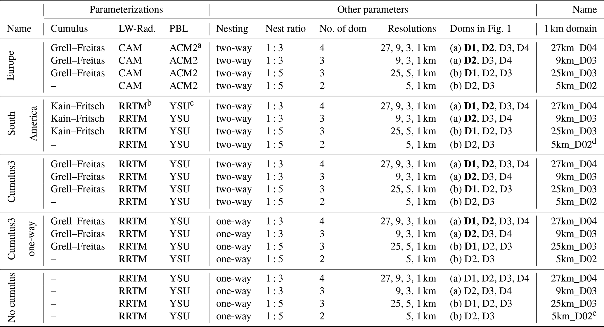
^a Asymmetric Convection Model Version2. ^b Rapid Radiative Transfer Model. ^c Yonsei University. ^d This simulation is identical to the last one in “Cumulus3” and therefore it is only shown related to the Cumulus3 parameterization option in Figs. 3, 4, and 5; ^e This simulation is identical to the last one in “Cumulus3 one-way”, and therefore it is only shown related
to the Cumulus3 one-way parameterization option in Figs. 3, 4, and 5.

2 Model configuration and data

2.1 WRF Model

We adopt the numerical weather prediction model WRF (version 3.8.1; Skamarock et al., 2008) to obtain fine-scale and local precipitation patterns. This model allows us to dynamically downscale initial and boundary conditions, which in this study are provided by ERA5 reanalysis. To determine an optimal setup for Kenya, and the Mount Kenya area in particular, we test different parameterization schemes, focusing on cumulus parameterizations, with two different model setups and nesting ratios. The experiments are described in more detail in the following and are summarized in Table 1. The experiments are all run for the same period of time, i.e. the year 2008, except for a single experiment that is repeated for the year 2006 to evaluate the robustness of the results for 2008 under different climate conditions. To permit the soil and the atmosphere to adjust to the initial conditions, we allow for 2 months of spin-up. Since the soil variables are well equilibrated in the ERA5 data, the used spin-up time of 2 months in our simulations is enough to bring the soil and the atmosphere into an equilibrium. Previous studies (Angevine et al., 2014; Jerez et al., 2020; Velasquez et al., 2020) back up the idea that rather short spin-up periods are enough for variables such as temperature or precipitation to reach the equilibrium in WRF, but for soil moisture longer periods are recommended (a few months). This means that the simulations start on 1 November 2007 and end on 31 December 2008.

Figure 1 The two different nesting settings for the sensitivity experiments are depicted. The four domains (D1 = 27 km, D2 = 9 km, D3 = 3 km, D4 = 1 km) of the nesting ratio 1:3 are shown in row (a), with the topography of the innermost nest D4 in the right panel. The three domains (D1 = 25 km, D2 = 5 km, D3 = 1 km) of the nesting ratio 1:5 are shown in row (b), with the topography of the innermost nest D3 in the right panel. The grey shading indicates elevation in metres above sea level using the WRF topography Global Multi-resolution Terrain Elevation Data (GMTED2010) provided by USGS. The location of the weather station data is provided in D4, and a more detailed description of each station is available in Table 2. The black star in D4 indicates the summit of Mount Kenya. Note that at least 30 grid points from the edge of the boundaries of an inner domain to the limit of an outer domain are used to avoid effects from the relaxation zone (spanning five grid points) between two nests (Rummukainen, 2010).

Two different nesting ratios, i.e. 1:3 and 1:5, have been used in different model domain settings to estimate the effect of the nesting ratio on the modelled precipitation and temperature (see Fig. 1). For the nesting ratio of 1:3, a four-domain (i.e. 27, 9, 3, 1 km horizontal resolution) and a three-domain (i.e. 9, 3, 1 km horizontal resolution) setup have been tested. In addition, the 1:5 nesting ratio is run with two different setups, i.e. a three-nested (25, 5, 1 km horizontal resolution) and two-nested domain setup (5, 1 km horizontal resolution). To test if the coarser setups affect the representation of precipitation and temperature over the study area, simulations with a coarser and finer parent grid are performed. This is because for the coarser setups the downscaling resolution is very similar to the one of ERA5, which provides the initial and boundary conditions. Such coarse spatial resolutions in the outermost domains are tested because the final goal is to also apply the WRF setup to climate simulations, which normally have a coarser resolution (around 100 km) than reanalysis data (around 30 km for ERA5). In that case, a climate simulation with a parent domain starting at 9 or 5 km is not possible. Nevertheless, the parameterizations are tested using ERA5 as boundary condition in order to be able to compare the simulations against observations of the year 2008. Note that in the simulations with a reduced number of nests (three domains instead of four for the 1:3 ratio, and two instead of three for the 1:5 ratio), the parent domain always corresponds to the second domain of the experiment with one nest more (Table 1). All simulations have 49 vertical eta levels up to 50 hPa and an innermost domain located over Mount Kenya with 1 km horizontal resolution. When comparing the different sensitivity experiments in the results (Sect. 3), the focus is always on the innermost domain of all the simulations. To save some computational costs, an adaptive time step is used, which is between 54 and 810 s in the outermost domain for the 1:3 ratio experiments and between 50 and 750 s for the 1:5 ratio. For the smaller domains, the time steps are reduced by the factor of the nesting ratio. A small sensitivity test, starting the simulation twice from the same restart file, indicates that the simulation is also reproducible with an adaptive time step.

Different physical parameterization schemes have been tested to optimize the representation of precipitation over Kenya. Tests have been done by varying the cumulus, the longwave (LW) radiation, and the planetary boundary layer (PBL) parameterization schemes. For cumulus parameterization, the Kain–Fritsch (Kain, 2004) and the scale-aware Grell–Freitas ensemble (Grell and Freitas, 2014) schemes have been used in the domains with resolutions >5 km, and one experiment is performed without using any cumulus parameterization in all of the domains. Note that the cumulus parameterization is switched off in all experiments for domains with horizontal resolutions ≤5 km. The LW radiation scheme has been varied between the Rapid Radiation Transfer Model (RRTM; Mlawer et al., 1997) and Community Atmosphere Model (CAM; Collins et al., 2004). The two first-order non-local-closure PBL schemes of Yonsei University (Hong et al., 2006) and the second version of the Asymmetric Convection Model (Pleim, 2007) have been tested. Table 1 provides a summary of the used parameterizations for each experiment and the exact setting can be found in the namelist files on Zenodo (see the code and data availability section). The rest of the parameterization options are kept constant throughout the different experiments, i.e. WRF single-moment 6-class scheme (Hong and Lim, 2006) for microphysics, Dudhia shortwave (SW) scheme for the SW radiation (Dudhia, 1988), and the Noah–MP land surface model (Niu et al., 2011; Yang et al., 2011) to describe surface processes. In all the simulations the lake model is turned on. The 1-D physically based lake model (Subin et al., 2012) helps to simulate lake internal processes and interactions at the surface of the lake with the atmosphere (Gu et al., 2015). It increases the eddy diffusivity, and it thus also strengthens the heat transfer in the lake column (Gu et al., 2015). This is considered to be beneficial for the description of the lake surface temperature, which again helps to better represent evaporative effects and thus precipitation over the lake and in the surrounding areas. A comparison of one simulation with the lake model turned off and one including the lake model reveals that the lake model is slightly beneficial for representing temporal and spatial precipitation patterns around Mount Kenya. Hence, the experiment without lake model is not presented in the following analysis. Please note that the aforementioned parameterization options are selected from an even larger set of experiments not included in this paper and are only tested with one nesting ratio and four nested domains. In addition, a simulation with the latest version of the model (V4.2.1) was run. However, it showed that the included improvements are not enough to reduce the root-mean-square error (RMSE) and to improve the temporal correlation against the weather station data compared to the other sets of experiments. It further indicates that model versions and compilers can impact the simulations performed with WRF. Consequently, it has not been included in the analysis presented here.

As already shown in Table 1, each experiment obtained a name, chosen based on the area used in the literature or on the main parameterization that it employs. The “Europe” experiment is based on the parameterization options used with WRF over Europe in previous studies by the authors (Messmer et al., 2017) but also including some updated schemes such as the Noah-MP land surface model. “South America” is based on the parameterizations used for the optimal simulation of storms over the central Andes (Zamuriano et al., 2019). The remaining “Cumulus” experiments are similar to the configurations applied over East Africa in previous studies (Pohl et al., 2011; Otieno et al., 2019), but they include the updated Noah-MP land surface model and changes in the cumulus scheme option (option 3 in WRF – “Cumulus3” experiment) or no use of cumulus parameterizations at all (“No Cumulus”). The No Cumulus experiment is motivated by a recent study (Vergara-Temprado et al., 2020) that shows some improvements in resolving convective precipitation explicitly compared to parameterized convection in horizontal resolutions of around 25 km. The difference between the Cumulus3 and “Cumulus3 one-way” is the communication between the parent and the respective child nest. In the one-way nested options, results from the inner domain are not overwritten on the parent grid, while this is the case for two-way nested domains. Note that the two-domain simulation starting at 5 km horizontal resolution is equal for the Cumulus3 one-way and the No Cumulus experiment, as they differ only in the cumulus parameterization. As both in that particular simulation explicitly resolve convective processes, the simulations are identical and will be presented as Cumulus3 one-way. This is also the case for the experiments South America and Cumulus3, as they both explicitly resolve convective processes in simulations starting at 5 km horizontal resolution. Thus, both experiments are also identical and will be presented as Cumulus3.

2.2 ERA5

ERA5 is the latest reanalysis provided by the European Centre for Medium-Range Weather Forecasts (ECMWF). At the moment, it is available from January 1979 until 3 months before present (Copernicus Climate Change Service, 2017). ERA5 provides different variables on the surface and various pressure levels with an hourly output. Nevertheless, we use 6-hourly data for our boundary conditions. The data are available globally on a 0.25^∘ horizontal grid spacing and use 137 vertical model levels. A vast number of observations and satellite data are assimilated to the ERA5 gridded data using the integrated forecasting system cycle 41r2. A total of 24 vertical pressure levels were fed to WRF (1000, 925, 900, 850, 800, 775, 750, 700, 650, 600, 550, 500, 450, 400, 350, 300, 250, 200, 150, 100, 50, 30, 20, 10 hPa).

As stated before, our analysis will focus only on the year 2008, although 2006 is used to test the performance of the best setting using a different year. Compared to the climatology of Kenya for the year 1981–2010, the year 2008 is one of the warmer years, but when considering the constant warming since the beginning of the current millennium, it can be considered as a new normal (Fig. 2a). The analysis of the detrended data also supports this (not shown). In terms of precipitation, 2008 is on the dry side compared to the climatology (Fig. 2b), but it is a year with two clear rainy seasons, the long rains, and the short rains (Fig. 2c). Additionally, the year 2006 is selected as it is rather wet compared to the year 2008.

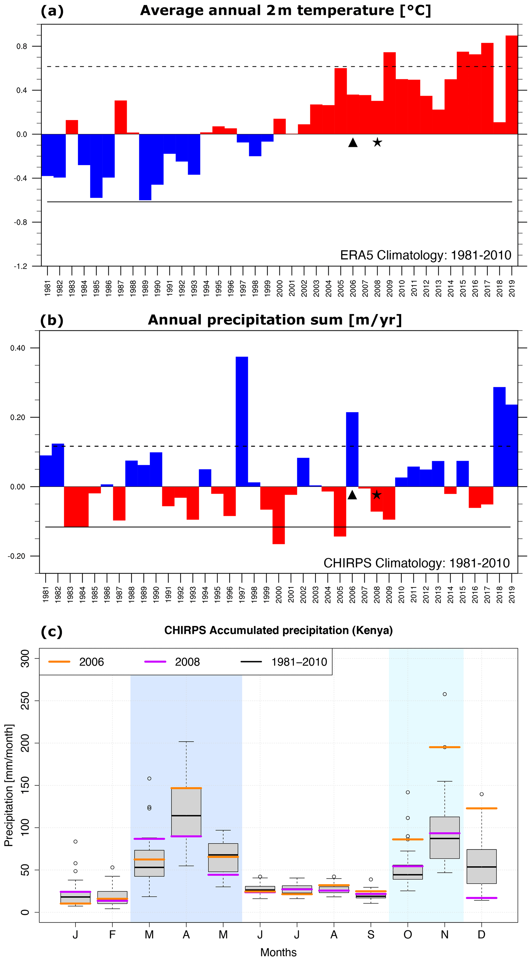
Figure 2 Annual anomalies of mean 2 m temperature (in ^∘C) from ERA5 (Copernicus Climate Change Service, 2017) (a) and of precipitation (in metres per year) from CHIRPS (Funk et al., 2015) (b). The anomalies are calculated with respect to the climatological mean of the years 1981 to 2010. The stippled (straight) lines illustrate plus (minus) 1 standard deviation. Monthly accumulated values of precipitation (in millimetres per month) for the selected year 2008 (in purple) and 2006 (in orange) compared to the climatology (1981–2010, in grey, using a box and whisker plot) are shown in (c). All values are means over the territory of Kenya in each subplot. The whiskers extend to the value that is no more than 1.5 times the interquartile range away from the box. The values outside this range are defined as outliers and are plotted with dots. The dark blue and light blue shading indicate the long rains and short rains, respectively.

2.3 Observational data sets

To analyse the output of the WRF simulations and to identify the best parameterization options, the downscaled product must be compared to some independent observational data sets. Hence, the precipitation results are compared to ERA5, three satellite-based data sets and independent weather station measurements. For temperature, the results are compared to ERA5. A comparison to the temperature data of Climatic Research Unit (CRU) data has also been performed, but the patterns are very similar to ERA5 and are therefore not shown here. Please note that the gridded data sets are bilinearly interpolated (Climate Data Operator (CDO); Schulzweida, 2019) to the grid of the WRF domain that it is compared to, and the nearest point to the station is considered afterwards. Consequently, small differences can appear in the values related to the gridded observational data sets. However, when the pattern correlation is calculated against gridded data sets, the grid of this data set is taken as a reference, and the WRF simulations are bilinearly interpolated to that grid. In the following, the different products are described in more detail.

2.3.1 Tropical Rainfall Measurement Mission (TRMM)

The Tropical Rainfall Measurement Mission (TRMM) comprises several data sets based on satellite data, and it is provided by NASA and the Japanese Aerospace Exploration Agency (JAXA). In this study we use the gridded data product TRMM 3B42 for precipitation estimates. Note that we use the research-grade TRMM 3B42 and not the near-real-time version, as the first is considered to be more suitable for research (Liu, 2015). Version 7 of TRMM 3B42 (TMPA 3B42 v7) is a combined product and merges satellite rainfall estimates with gauge data. To obtain the 3-hourly precipitation estimates, radars are calibrated to the microwave imager precipitation, which should result in a 3 h microwave-only best estimate. In a next step, infrared precipitation is calibrated to the microwave product to fill regional gaps. Finally, the 3-hourly estimate is summed up to monthly values and recalibrated using a rain gauge analysis (Huffman et al., 2007, 2010). This monthly surface precipitation gauge analysis is obtained from the Global Precipitation Climatology Centre (GPCC). The result is a Level-3 product with 3-hourly temporal and 0.25^∘ × 0.25^∘ spatial resolution on a quasi-global (50^∘ N–50^∘ S) grid. With this resolution the TRMM 3B42 data is very similar to ERA5. TRMM 3B42 is available for the period 29 February 2000 to 2 January 2020.

2.3.2 IMERG

The Integrated Multi-satellitE Retrievals from GPM (IMERG) provides a multi-satellite product, currently available in its sixth version. It is the successor to the TRMM data set. Several products with different latency periods are available, but for this study we make use of the final product, which is suitable for scientific purposes. Similar to TRMM, several microwave measurements are used to estimate precipitation, and it is further calibrated against instrument products. The half-hourly precipitation estimates are further recalibrated with a CMORPH Kalman filter and the PERSIANN Cloud Classification System artificial neural network. The product is finally adjusted to the monthly GPCC rain gauge measurements and is available in half-hourly time steps and on a spatial resolution of 0.1^∘ × 0.1^∘ (approximately 10 km × 10 km). The available time period is from June 2000 until present.

2.3.3 CHIRPS

The Climate Hazards group Infrared Precipitation with Stations (CHIRPS V2.0) provides a high-resolution data set with daily rainfall amounts (Funk et al., 2015). The 0.05^∘ spatially resolved data are available for parts of the mid-latitudes and the tropics (50^∘ S–50^∘ N). The data set is generated using thermal infrared precipitation products from different institutions. To calibrate global cold cloud duration rainfall estimates, the Tropical Rainfall Measuring Mission Multi-satellite Precipitation Analysis version 7 (TMPA 3B42 v7) is used (Funk et al., 2015). In a first step, the World Meteorological Organization's Global Telecommunications System (GTS) rain gauge data, which are relatively sparsely available, are combined with cold cloud-duration-derived precipitation estimates. In a second step, the best available weather station data are combined with cold cloud-duration-based precipitation to get a product that on a monthly mean is similar to those produced by the GPCC or the CRU from the University of East Anglia (Funk et al., 2015). Note that IMERG and TRMM also recalibrate their monthly output to results obtained from GPCC, and CHIRPS is based on the same satellite product as TRMM, hence the three data sets used for the model verification are not fully independent of each other, especially when monthly sums are investigated.

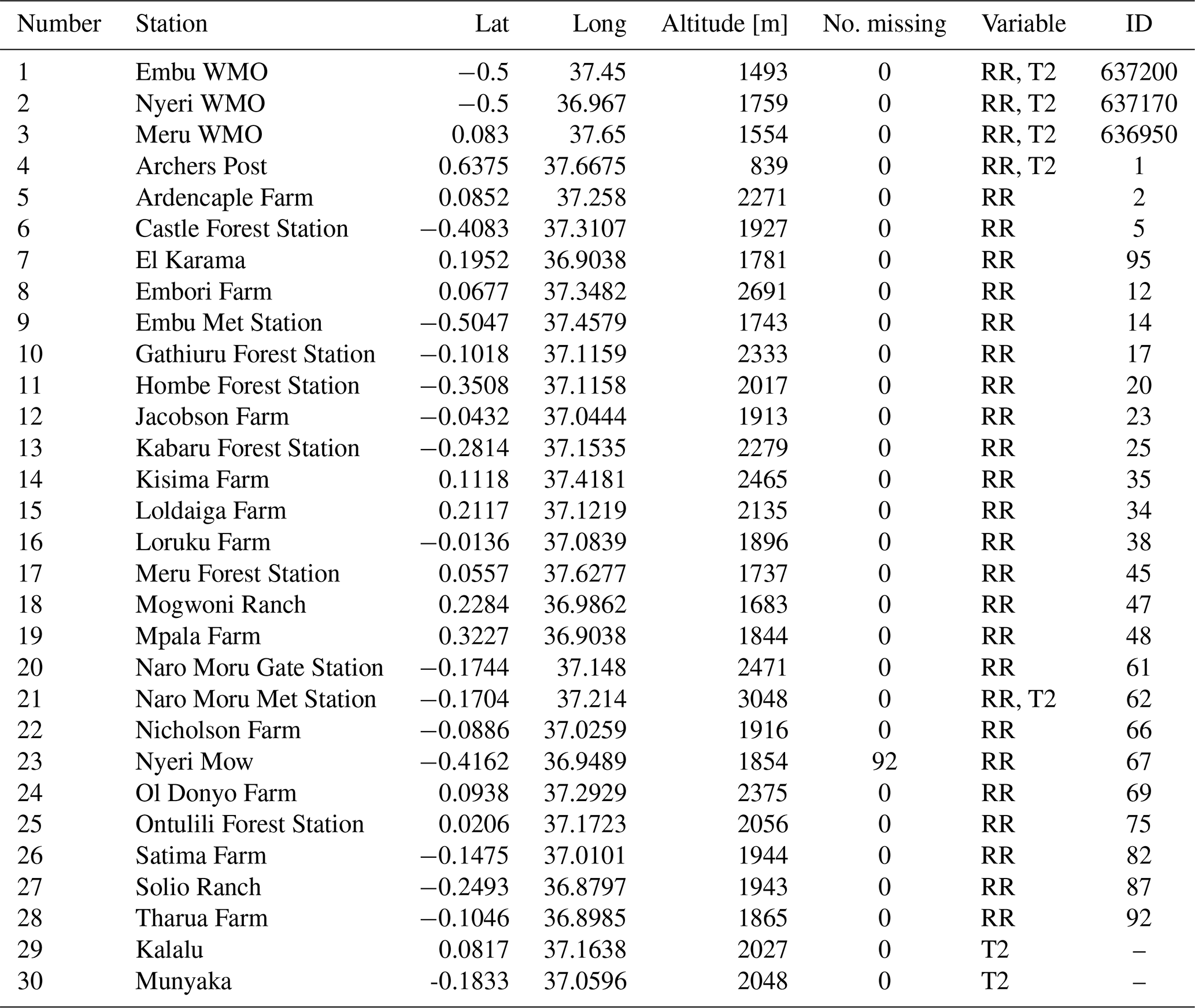
Table 2 Weather station information: station number used in our study (labels in Figs. 1, 6, and 7), station name, location (latitude and longitude), altitude (in metres above sea level), number of missing values, variables available, and station ID from WMO (first three lines) or from Table 1 in Schmocker et al. (2016). RR stands for precipitation and T2 for 2 m temperature.

2.3.4 Weather station data

Compared to other tropical areas in Africa, Kenya (and especially the area around Mount Kenya) is covered by a comparably large number of weather station data with long precipitation measurement series. Many of these measurement series are maintained by farmers. Thanks to the support and involvement of the University of Nairobi and University of Bern, these series are still available today (Gichuki et al., 1998; Liniger et al., 2005; MacMillan and Liniger, 2005). In addition to private stations, there are also some that are operated by the government of Kenya, i.e. the Kenya Forest Service or the Kenyan Meteorological Department. For precipitation, we use data from 28 stations that have been quality controlled by Schmocker et al. (2016). Table 2 provides some information on the stations used in this study, but for more detailed information the reader is referred to Table 1 in Schmocker et al. (2016). The station ID in both tables are identical to ease comparison. We obtained four stations with temperature records from the Social Hydrological Information Platform (SHIP), which is associated with the Water and Land Resources Centre (WLRC) project of the Centre for Training and Integrated Research In ASAL Development (CETRAD). Three additional stations for precipitation and temperature are included in the World Weather Records (WWR) database from the World Meteorological Organization (WMO). These are the three first lines of Table 2. Note that the weather station data have not been adjusted to the height of the model topography, as the differences in height are in the range of a few metres. The maximum difference between the station and model height is around 60 m, and hence the maximum discrepancy between station and modelled temperature is around 0.4 ^∘C if we consider the standard environmental lapse rate of 6.5 K km⁻¹ (Barry, 2008). Additionally, the quality control performed by Schmocker et al. (2016) suggests that several stations are only suitable for monthly analyses. As the number of stations in the innermost domain should stay as large as possible, the study is mainly based on the monthly resolution. Most of the weather stations are located on the northwestern slopes of Mount Kenya, and they are rather scarce to the southeast of it, which could affect the reliability of our results. However, we reduce this uncertainty by also comparing our results against several gridded observational data sets.

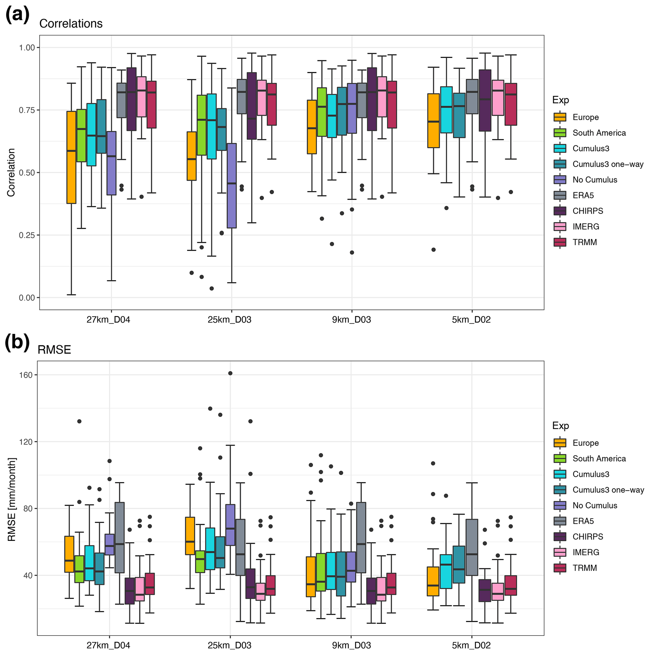
Figure 3 The temporal correlation (a) and root-mean-square error (RMSE) (b) between the annual cycle for the year 2008 of measured and simulated monthly precipitation sums at the nearest grid point to the station's location shown for the different parameterization options (see legend to the right, Table 1) and grouped by the different nesting options and number of nests. The box and whisker plots show the values in relation to 28 stations for the different domains with 1 km spatial resolution. The whiskers extend to a value that is no more than 1.5 times the interquartile range away from the box. The values outside this range are defined as outliers and are plotted with dots.

3 Results

3.1 Sensitivity of precipitation

3.1.1 Temporal analysis

To investigate the sensitivity of simulated precipitation due to different parameterization options of the WRF model, we first show the annual cycle based on monthly means. Thereby, the sensitivity simulations with WRF and the three gridded observational data sets are compared to in situ data from weather stations (see Table 2 for more details). To compare gridded data with point measurements at weather stations, the grid point that is closest to the corresponding latitude and longitude of the weather station is considered in the WRF simulation and the gridded observations. Two performance measures for each weather station are calculated and summarized in box and whisker plots (Fig. 3): the temporal correlation and the RMSE. For correlations we use the Spearman correlation, which is a rank correlation that is suitable for the small sample sizes that are explored here. Additionally, the standard deviation of each data set is compared to the one extracted from the weather stations (not shown). Several different gridded observational data sets are employed here to compare the sensitivity simulations and to classify which WRF setting performs best. As not only the weather station data but also the gridded observational data sets are subject to a range of uncertainties, we rely on more than one product. Note that because the gridded data sets are bilinearly interpolated to the respective WRF grid, small differences can appear in the values of temporal correlations and RMSEs of each setup, and hence the shape of bars corresponding to these data sets in the box and whisker plots can also look slightly different.

The temporal correlations show that the observational data sets (ERA5, TRMM, and especially IMERG) are well correlated (Fig. 3a). This is expected as the data are not fully independent from each other. IMERG has the best correlation with the highest median but also with the smallest spread. Generally, the observational datasets show a good correlation of around 0.8 in the median value. The fact that IMERG and the weather station data show such a good agreement further confirms the quality of the latter. The temporal correlations of the sensitivity simulations show a strong dependence on the nesting options. The simulations with fewer nests (right part of Fig. 3a) exhibit a higher correlation and a smaller spread than the two simulations that have one additional nest (left part of Fig. 3a). In particular, the No Cumulus simulation and the Europe setup show a poor performance in the temporal correlation. Note that the poor performance of the No Cumulus setup can only be observed in nesting options with a larger number of domains, i.e. setups with a parent grid of 27 or 25 km. The fact that the nesting option is important here suggests that with fewer domains (only three instead of four nests for the 1:3 ratio and two instead of three for the 1:5 ratio), the simulation in the innermost domain is still more strongly influenced by the boundary conditions of the driving data, i.e. ERA5. Thus, the simulations with fewer nests cannot evolve with the same freedom as the ones with more nests, resulting in a better temporal agreement of the simulations. This is especially clear in the No Cumulus simulation.

While all the gridded observational data sets yield a rather high temporal correlation, the RMSE of ERA5 is rather high compared to the ones of TRMM, IMERG and CHIRPS (Fig. 3b). A reason for this is that the precipitation in ERA5 is independent of the weather station data, as precipitation is not assimilated into this product. Otherwise, the RMSE shows similar results to the correlations for both the gridded observations and the sensitivity simulations. Hence, the parameterization of the simulation is only of minor importance compared to the nesting options. Similar findings are obtained when using the standard deviation (not shown). Here, the WRF simulations are generally within the range of the standard deviation observed in the weather station data, except for the Europe parameterization in the nesting options with fewer nests. In that case, the standard deviation is strongly underestimated, indicating that the variability of precipitation is not fully captured. Additionally, the standard deviations of the gridded observational data sets are smaller than the ones of the weather station data, which is owed to the coarser resolution of the first. At finer temporal resolutions than monthly sums, these temporal correlations and RMSEs reproduce the differences between the experiments as discussed for monthly means. However, using finer timescales leads to a general reduction of the correlation coefficients and an increase in RMSEs. This is expected, as the variability is higher and because it is more and more challenging for the model to capture the exact timing of precipitation (not shown).

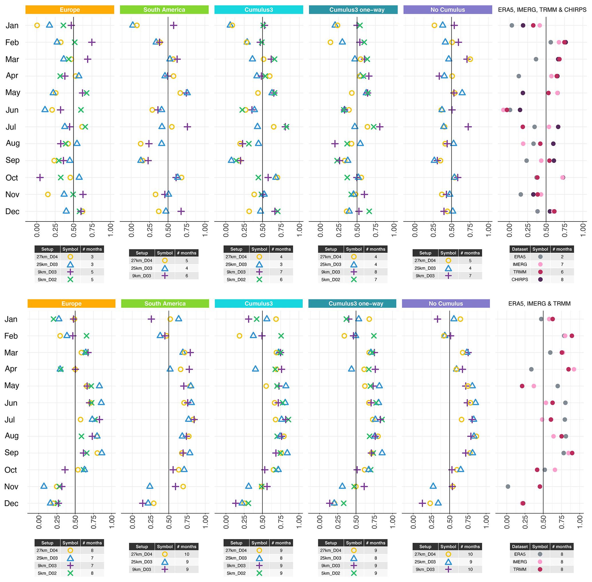
Figure 4 Pattern correlation of monthly precipitation sums for the year 2008 between weather station data and the respective WRF simulation (upper row) and between CHIRPS and the respective WRF simulation (interpolated onto the CHIRPS grid, lower row). The different panels indicate the different parameterization options (Table 1), and the symbols stand for the different nesting options. The labelling of the symbols is given in the table below each panel, along with the number of months (# months) in which the nesting option obtain correlation patterns above the reference value of 0.50 (a moderate correlation used to visually evaluate the performance of nesting options). The last panel on each row represents the gridded data sets used throughout the paper. Even if the gridded data sets are interpolated onto different domains for each independent setup, here only one setting is shown (27km_D04, only first row). The rest was omitted as only marginal changes can be observed.

3.1.2 Pattern correlation analysis

Since the temporal correlation and the RMSE do not clearly define which parameterization option of WRF delivers the best results for precipitation in the region around Mount Kenya, we investigate the pattern correlation of the simulations compared to weather station data in a first step and to the gridded observational data set CHIRPS in a second step. Figure 4 shows the pattern correlation between the WRF-simulations and the weather station data for each month in the first row. The different columns indicate different parameterization options, and the symbols within each panel show the nesting option. The vertical black line in each panel is equal to a correlation coefficient of 0.5. This value is a moderate correlation and still explains roughly 25 % of the variance, but it is a visual support to more easily determine which simulations and nesting options perform better than others. The number of months that are equal to or exceed this limit of 0.5 in correlation are counted and summed up in the table below each panel (“# months” column).

The gridded observational data sets agree reasonably well in terms of the spatial pattern of precipitation, except for ERA5. The fact that ERA5 shows a poor correlation with the weather station data is because the domain is located over steep terrain, where a high resolution is needed to resolve precipitation patterns appropriately. CHIRPS has the highest spatial resolution and shows a slightly better pattern correlation than IMERG (especially in June), and hence we have decided to also compare the WRF simulations against the CHIRPS gridded data set (second row of Fig. 4). Additionally, CHIRPS shows high correlations and low RMSEs in the temporal analysis. Similarly to the temporal correlation, the simulations with fewer nests obtain a better pattern correlation compared to the ones with an additional nest. The South America and the No Cumulus parameterizations show the highest agreement with the weather station data for the nesting options that have an additional nest, while clearly the Cumulus3 one-way option is the best of the simulations with fewer nests. Overall, the simulations have a better performance in the rainy seasons MAM and ON, while the dry months (and June in particular) are not very well captured by the model simulations.

Besides the comparison to the weather station data, the simulations and gridded observational data are compared to CHIRPS (see the second row of Fig. 4). As mentioned before, all the simulations were bilinearly interpolated to the grid of CHIRPS for this spatial analysis. The gridded observational data sets perform well compared to CHIRPS (including ERA5). Again this is expected as the data are not fully independent. The pattern correlation of the WRF simulations compared to CHIRPS are rather high in all the simulations. No clear difference between the different nesting options are evident. The South America and the No Cumulus options show the best agreement with CHIRPS in precipitation patterns, but Cumulus3 one-way also performs well. The Europe parameterization is clearly the worst, even if it shows one of the highest correlations in the dry months of June and July. This is because the Europe parameterization setup produces rather dry conditions over Africa, and hence the dry months are better represented compared to the others that simulate generally wetter conditions.

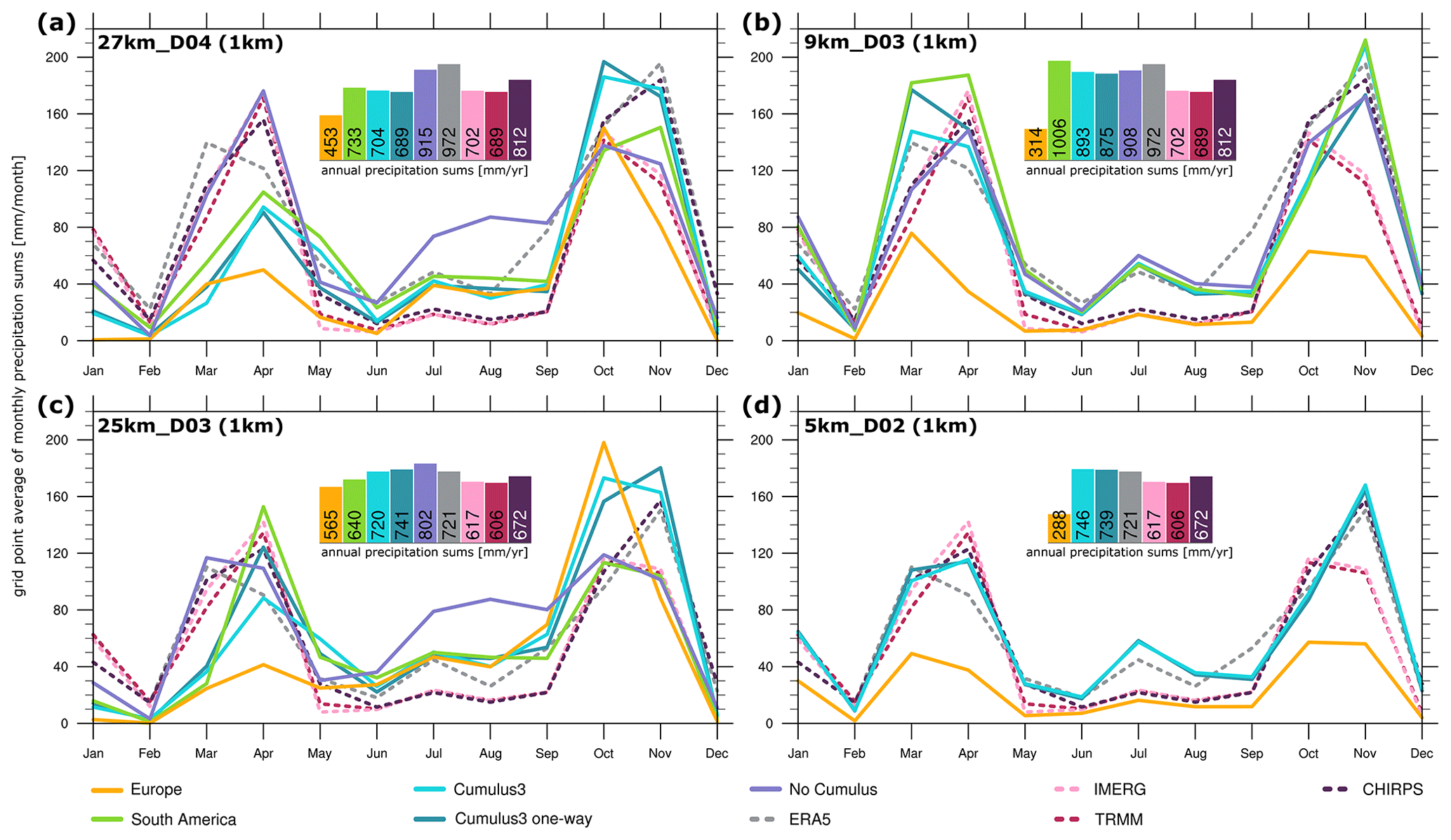
Figure 5 Grid point averages of monthly precipitation sums in millimetres per month for the year 2008 in the innermost domain (1 km) for each of the tested setups: 27 km (a), 9 km (b), 25 km (c), and 5 km (d). The five tested parameterization options are included, along with the driving reanalysis ERA5 and the three observational gridded data sets (IMERG, TRMM, and CHIRPS). All the gridded data sets are plotted with different shades of pink, while ERA5 is coloured in grey. The inset of a bar plot in each panel indicates the grid point average annual precipitation sum in millimetres per year for each parameterization option and gridded data set.

3.1.3 Annual cycle

To further understand how well the different parameterization and nesting options are able to represent precipitation around Mount Kenya, the annual cycle is plotted as grid point averages of monthly precipitation sums of the innermost domain (1 km; Fig. 5). Please note that the gridded observational data sets do not obtain exactly the same values for the different nesting ratios 1:3 (first row) and 1:5 (second row), as the domain sizes are not exactly equal. The innermost domain in the 1:5 nesting ratio setup is slightly bigger. The three gridded observational data sets TRMM, IMERG, and CHIRPS agree well and are considered the reference here because they show a good temporal and pattern correlation with the weather station data. This is true except for November, when CHIRPS records a much higher value in precipitation amounts than TRMM and IMERG. As CHIRPS shows one of the weakest pattern correlations in November compared to the weather station data, IMERG and TRMM should be considered the reference in this month. ERA5 also agrees, but the long rains (MAM) have the peak intensity a bit too early, while the intensity in the short rains (ON) is too intense on average. For the dry months, ERA5 also overestimates precipitation compared to the other gridded observational products. Overall, the gridded data sets come up with similar annual precipitation sums (see the inset of Fig. 5), except for ERA5, which shows a slight overestimation in annual precipitation sums. Comparing the monthly precipitation sums of the sensitivity simulations with the gridded observational reference, we find again that the Europe parameterization option is not well suited for this area as it is not able to correctly capture the two rainy seasons near Mount Kenya. The long rains show a clear deficit in precipitation, while the outcome of the short rains strongly depends on the number of nests. With fewer nests the short rains are also clearly underestimated but with an additional nest precipitation is either almost correct or is overestimated. The differences between the Europe setup and the others are related to the parameterization of the longwave radiation and PBL, which are both responsible for the reduction in precipitation amounts according to previous sensitivity tests with these parameterizations (not shown). The No Cumulus setup performs well in both wet seasons, but it overestimates precipitation during the dry season. The Cumulus3 options show a clear sensitivity of the precipitation amounts in the long rains to the number of nests, with a much better representation with fewer nests. In the short rains, the Cumulus3 options follow the curve of CHIRPS and therefore shows an overestimation. The fact that the Europe setting is not suited for this region becomes even clearer when including the annual precipitation sums. Except for the 25 km parent grid, the Europe setting captures only around 50 % of the annual precipitation, and hence it clearly underestimates the water availability. All the other settings perform similarly well on an annual basis (insets in Fig. 5). It is also noteworthy that the WRF model with the Cumulus 3 options is able to correct the overestimation obtained by ERA5, which is the driving data set of the simulations.

Figure 6 Monthly precipitation sums for (a) April 2008 (long rains), (b) November 2008 (short rains), and (c) June 2008 (dry season) in millimetres per month for the innermost domain (1 km) of the four-domain nested setup, with an outermost domain of 27 km resolution and a nesting ratio 1:3 for the different parameterization setups (see Table 1). Weather station data are described in Table 2. The white star indicates the summit of Mount Kenya, and missing values are marked in black. The numbers in the lower-right corner of each panel indicate the spatial correlation with respect to the stations (upper line) and CHIRPS (lower line).

3.1.4 Precipitation patterns

Another measure used to identify the best setup of WRF for this region is the precipitation patterns of the WRF simulations. Due to the aforementioned motivation to use the tested settings in a climate simulation, in the following the simulation of the innermost domain (D4; 1 km) with the parent domain of 27 km horizontal grid spacing and a nesting ratio of 1:3 is presented. Note that the simulations with a 25 km parent grid and a nesting ratio of 1:5 show similar results and are hence not shown here. To present the results, months within the three main seasons are presented, i.e. the long rains, short rains, and the dry season. April (Fig. 6a) is chosen as it is in the midst of the long rains. November (Fig. 6b) is selected as it is within the short rains and has a larger spread between the different experiments than October. Finally, June (Fig. 6c) represents a month in the dry season and shows stronger deviations compared to station data. As CHIRPS is the data set that shows the best agreement with the weather station data (as shown in Fig. 4) and because it also shows the highest resolution and detail, in the following only this gridded observational data set is presented as a reference. Additionally, the Europe experiment is discarded because of its weak performance in the previous analyses.

In April, the precipitation from CHIRPS is similar to the measured amounts of precipitation, with the exception of a small region located to the north of Mount Kenya where precipitation is overestimated by this gridded data set (Fig. 6a). Bearing in mind that the observational data set is also subject to some uncertainties, the South America parameterization shows similar precipitation amounts and patterns along a diagonal band from southwest to northeast, lacking some of the precipitation southeast of Mount Kenya, as indicated by CHIRPS. The northern part of the domain seems to be too dry compared to CHIRPS, but stations along the northern slope of Mount Kenya agree relatively well. The other three setups manage to produce a precipitation pattern as observed in CHIRPS. Nevertheless, the No Cumulus parameterization is too wet, especially in the northwestern part of the domain, and the steep gradient from high precipitation rates in the vicinity of Mount Kenya to dryer conditions to the northwest of it is not well captured. The two Cumulus3 parameterization options capture this pattern the best, including also some finer details along the right and bottom boundaries of the domain.

CHIRPS also captures the precipitation pattern quite well in November, with some deviations compared to the weather station data south and northwest of Mount Kenya (Fig. 6b). South America captures the precipitation amounts of the stations quite well, but the pattern shows some deviations compared to CHIRPS, especially in the northwestern corner of the domain. The two Cumulus3 and the No Cumulus options are able to capture the patterns well with some overestimation in the simulations driven by the first option and a slight underestimation in precipitation amounts for the latter parameterization option. Given the uncertainty range within the observation-based data, it cannot be expected that a single sensitivity simulation can agree with all the stations or with one of the gridded observational data sets.

June is clearly much drier than April, and CHIRPS also records too much precipitation compared to the weather station data (see Fig. 6c). Given the uncertainty range of the observation-based data, the South America parameterization option does not fully agree with CHIRPS in terms of the general pattern, as no dry corridor in the east is simulated and precipitation is overestimated at most of the stations. This is also true for the No Cumulus parameterization option, but here the pattern agrees better, with a clear overestimation in precipitation amounts. Cumulus3 and Cumulus3 one-way again result in the best pattern, rendering it difficult to choose between the two, as some stations are better in one setting and other stations are better described in the other. Since one-way nesting does not overwrite the solution of the corresponding parent grid, this option should be preferred over the two-way nesting option. It allows us not only to focus on the innermost domain but also investigate the larger-scale picture without any disturbances within the domain.

All the WRF simulations reasonably resemble the precipitation pattern over Mount Kenya in the year 2008. The Europe setting provides the worst performance and too dry conditions throughout the whole year. The No Cumulus parameterization and the Cumulus3 options provide the best performances throughout the analysis. The fact that the No Cumulus option is generally too wet allows us to define the Cumulus3 one-way option as the best for our purpose. Note also that the No Cumulus parameterization option produces a patchy picture in the outermost domain with monthly sums, which is a clear sign of a structural problem, i.e. convection always being induced at the same location (not shown), which is rather unrealistic. Hence, this simulation is also unsuitable for a larger-scale analysis of precipitation and precipitation changes in a warmer climate. Even if we are only interested in the results on a kilometre-level scale, it must be noted that the timing (not necessarily the amount) of the peak precipitation rates on a sub-daily basis are captured more realistically with respect to IMERG by the No Cumulus experiment compared to the other setups. This is only true for domains where the others use a cumulus parameterization (e.g. D2; see Fig. S1 in the Supplement).

3.1.5 Evaluation of performance under wet climatic conditions: year 2006

With the best parameterization option (Cumulus3 one-way) and the setup with a parent domain of 27 km horizontal grid spacing and a nesting ratio of 1:3, a further experiment is performed in order to test the applicability to other years. Therefore, the rather wet year 2006 is selected, as indicated in Fig. 2b. Here, we no longer compare the results to TRMM, as IMERG and CHIRPS provide finer resolved precipitation information. The temporal correlation of monthly precipitation sums with respect to the station data (see Fig. S2a) is even slightly higher in 2006 than in 2008, while ERA5 performs worse in 2006 than 2008. CHIRPS and IMERG perform similarly in both years. The RMSE of all the different analysed precipitation data is slightly larger than in 2008 but still shows a good performance (see Fig. S2b). Both CHIRPS and IMERG show a similarly good pattern correlation with the station data in 2006 as in 2008. ERA5 shows also a similar behaviour in the 2 years, being not able to capture the main precipitation pattern of the stations. Cumulus3 one-way reflects the precipitation pattern against weather station data reasonably well (see Fig. S2c), with 7 months of higher correlations than 0.5, which is a clear improvement compared to 2008. The spatial pattern correlation with respect to CHIRPS (see Fig. S2d) results in values higher than 0.5 in 11 months, which none of the parameterization experiments reached in the year 2008. Only December is just below this limit, with a spatial correlation of 0.476.

Cumulus3 one-way captures the precipitation patterns (see Fig. S3) well, especially in the two rainy seasons of 2006, i.e. April and November. In April the northern part of the domain is a bit too dry compared to the stations and CHIRPS, while in November the eastern part is slightly too dry compared to CHIRPS and compared to the station data. In June, CHIRPS and WRF produce very similar patterns, but compared to the station data they are both too wet, especially on the northern foothills of Mount Kenya. All in all, this setting even shows a better performance in the wet year 2006 than in the slightly dry year 2008.

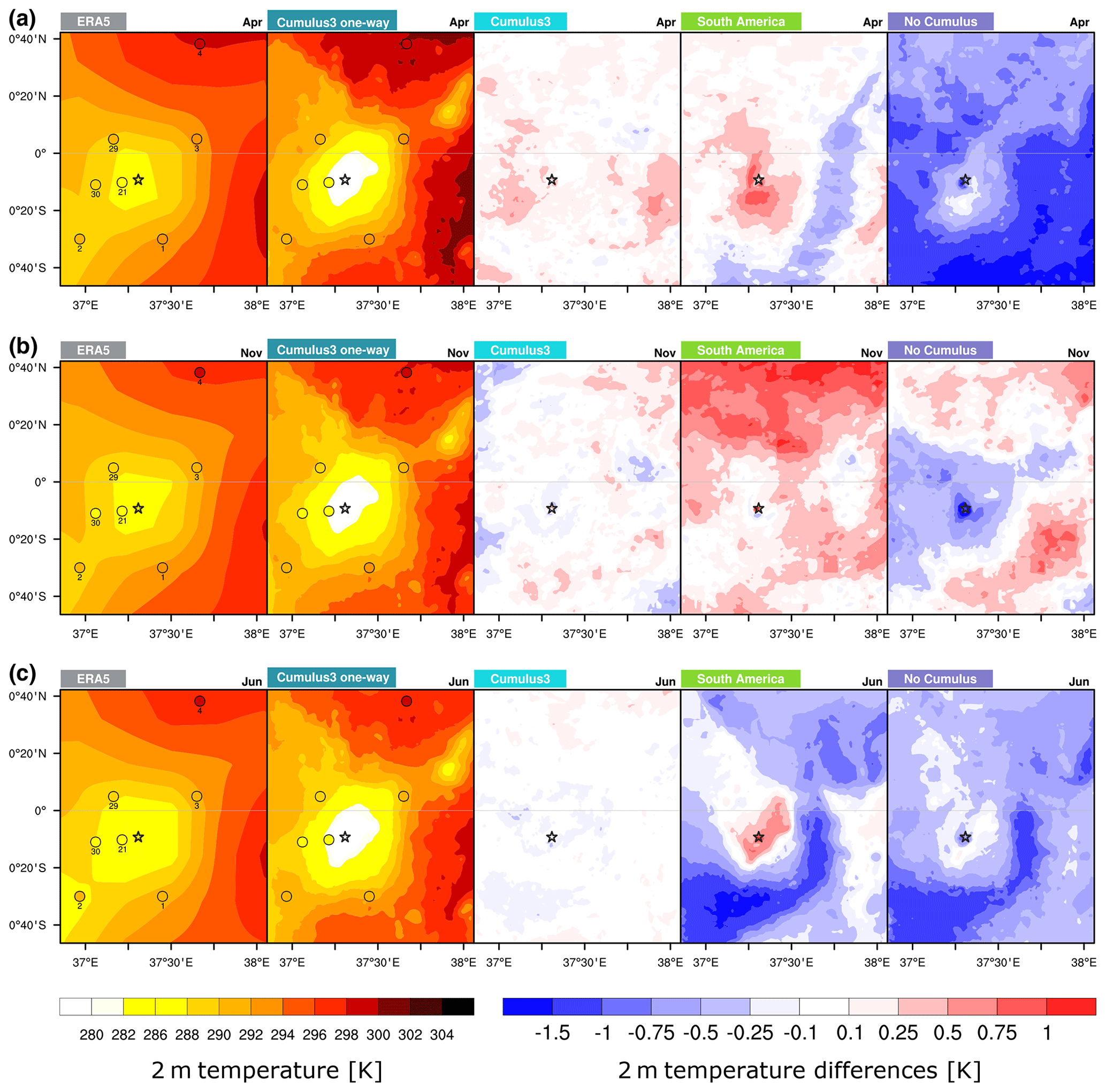
Figure 7 Monthly 2 m temperature averages for (a) April 2008 (long rains), (b) November 2008 (short rains), and (c) June 2008 (dry season) in K are shown for the innermost domain (1 km) of the nested four-domain setup, with the outermost domain of 27 km resolution and a nesting ratio 1:3 for the different parameterization setups (Table 1). Absolute values are given for ERA5 and the Cumulus3 one-way option. The others depict differences compared to the Cumulus3 one-way option. Weather station data are described in Table 2. The black star indicates the summit of Mount Kenya.

3.2 Sensitivity of temperature

Once we have investigated the sensitivity of simulated precipitation due to different parameterization options, we focus on temperature. To do so, the sensitivity simulations with WRF, except for Europe because of its bad performance in precipitation, are compared to the driving reanalysis ERA5 and the in situ data from weather stations (see Table 2 for more details). To measure how the different settings simulate the temperature near Mount Kenya, the 2 m temperature patterns are evaluated. The same months are selected for temperature as for precipitation: April (Fig. 7a) and November (Fig. 7b) within the long and short rains, respectively, and June (Fig. 7c) within the dry season. In order to highlight the differences between the sensitivity experiments, only the absolute values of the gridded data sets and the Cumulus3 one-way experiment are depicted. For the remaining sensitivity experiments, the anomalies compared to our best setting experiment are presented.

ERA5 temperature serves as boundary and initial conditions for the WRF simulation. Given this constraint, we expect a better representation of the simulated 2 m temperature than of precipitation. In addition, the region of interest is dominated by steep topography, which is directly related to temperature, and consequently strong gradients of temperature are expected near Mount Kenya.

It is not surprising that ERA5 represents temperature relatively similarly and independent of season (rainy or dry) as Kenya is located at the Equator. ERA5 describes the orography of the domain clearly and most of the few weather station data agree well with ERA5, but the WRF simulation Cumulus3 one-way produces a better temperature profile, which is mainly owed to the better resolution and a more detailed characterization of the topography.

In April (Fig. 7a), the two Cumulus3 simulations have a very similar representation of temperature, as the only difference is the communication between the nests. The difference for the South America experiment is mainly in the range of ±0.5 ^∘C, with positive anomalies over Mount Kenya and negative anomalies in the surrounding plains. In the case of the No Cumulus parameterization, strong negative anomalies are observed over the entire region, particularly in the southeastern corner where anomalies reach −2 ^∘C. This negative temperature anomaly is probably related to the overestimation in precipitation, as most of the domain obtains more precipitation than in the Cumulus3 one-way simulation. This excess in water can be transformed into latent heating through evaporation and can contribute to a cooling effect over the domain.

In November, the Cumulus3 one-way option overestimates the precipitation somewhat, which generally results in cooler temperatures compared to observations in some stations (e.g. stations 1 and 4 in Fig. 7b). As the other sensitivity experiments simulate a drier monthly climate in the plains especially, a positive temperature signal is found in these areas as well. Generally, the temperature differences between the experiments are again rather small and below 1 ^∘C.

The two Cumulus3 options are able to correctly simulate the observed temperature in June (Fig. 7c), and their differences are rather small (below ±0.25 ^∘C). The temperature bias for the South America experiment is higher in June than in April, but the patterns are similar (positive anomalies over Mount Kenya, but negative ones in the plains). Again, negative anomalies are simulated in the No Cumulus experiment, which could also be related to an increase in precipitation amounts, especially in the southeastern corner of the domain.

As described above, the differences in the patterns in the 3 months resemble the differences in precipitation to some extent; i.e. where more precipitation is simulated compared to Cumulus3 one-way, temperatures are reduced. One process which partly explains this is the transformation of energy into latent heating through evaporative processes. Where precipitation is comparably reduced to the Cumulus3 one-way parameterization, a warming is found. This is potentially due to energy that is transformed into sensible heating. Additionally, moisture advection and small differences in the description of cloud cover are additional relevant processes explaining some of the changes in temperature.

4 Summary and conclusions

The goal of this study was to find a setup for WRF in order to realistically simulate precipitation patterns and amounts over and around Mount Kenya at a kilometre scale. This task is challenged by the fact that this region has a complex topographic structure and is influenced by large-scale circulation controls, which leads to heterogeneous precipitation patterns. As this is one of the first studies to resolve the Mount Kenya region at such a fine scale, different parameterization options and combinations must be tested to obtain an optimal result for this area. We employ the WRF model and experiment with different combinations of cumulus (Kain–Fritsch, Grell–Freitas, no cumulus), LW (CAM, RRTM), and PBL (ACM2, YSU) parameterizations and with the number of nested domains and nesting ratios (1:3 and 1:5). The different simulations are not only compared to different gridded observational data sets, such as IMERG, TRMM, and CHIRPS, but also to a large number of weather station data operated by private farms, CETRAD, and the Kenyan government.

Correlating the annual cycle as monthly sums reveals that the gridded observations and the weather station data agree very well, indicating that the weather station data presented here are reliable. The temporal correlations further lead to the conclusion that if ERA5 is used as boundary conditions in a smaller and higher-resolved domain (i.e. simulations with one nest fewer) the simulation is more constrained, and hence the temporal correlation is better with a reduced number of nests. This result is mainly important for simulations driven with reanalysis data, as they capture most of the atmospheric circulation and processes well and are therefore reliable, which is not necessarily true for climate simulations. The No cumulus parameterization scheme is especially sensitive to changes in the number of nests in terms of temporal correlation. Concerning the nesting ratio, we are not able to distinguish between the two options, so either of the two is able to produce realistic results.

Also important for water availability in the area around Mount Kenya are the precipitation patterns and amounts. The objective pattern correlations indicate that fewer nests also result in a better spatial correlation, but when comparing against the most accurate gridded data set, CHIRPS, there is not much difference between the number of nests in spatial patterns. Compared to the temporal correlation, the No Cumulus parameterization results in rather accurate pattern correlations. The pattern correlation is a valuable tool to evaluate not only the sensitivity simulations but also the gridded observational data sets. The comparison to the weather station data reveals that CHIRPS yields a pattern closer to the weather stations. One important factor for this result is certainly the nominal resolution of the data, as CHIRPS reveals the finest precipitation structure of all the gridded observational data sets.

The Europe configuration obtains one of the worst temporal correlations and pattern correlations. The actual patterns within the innermost domain reveal that the Europe configuration is clearly too dry in both the rainy and dry seasons. The underestimation in precipitation can be attributed to both the LW and PBL parameterizations. However, not only are the precipitation amounts underestimated, the precipitation pattern is also not fully captured. The South America setting is more accurate when it comes to monthly precipitation sums in the rainy season, but it clearly has a wet bias in the dry season, and the precipitation pattern is also missing some details compared to CHIRPS. While the two Cumulus3 options and the No Cumulus option provide rather good precipitation patterns, the latter clearly overestimates the monthly sums. Hence, we conclude that the Cumulus3 one-way option is the best parameterization setting in WRFV3.8.1 for the area around Mount Kenya. The one-way nesting option is preferred over the two-way option, as the latter affects the representation of the domain when cumulus parameterization is turned off. Hence, with the one-way option, all domains and scales of the simulation can be integrated into the analysis.

The Cumulus3 one-way setting provides even better results for the year 2006 in terms of temporal correlations, and pattern correlations and precipitation amounts show a good agreement with respect to CHIRPS and to the weather station data. This result further supports the robustness of the results presented here, as not only rather dry years but also very wet years are reasonably well captured by this WRF model setup and driven with ERA5.

Similar to other studies, we also find an overestimation in precipitation compared to observations (Cook and Vizy, 2013; Williams et al., 2015). Nevertheless, with our sensitivity experiments we identify a parameterization setting that represents precipitation amounts rather well in the rainy seasons, while a wet bias remains in the dry season. Certainly, the very high resolution of our simulations helps to better represent the pattern not only of precipitation but also of temperature, resembling findings of Kerandi et al. (2017). It is not surprising that a high resolution can add value in the representation of precipitation and temperature, as this region is located within complex topographic structures.

Having found the optimal setting for the Mount Kenya area, climate change simulations can be performed. These allow to get a detailed picture of the climate sensitivity in this area and the possible changes in water availability and the actual warming in the area. Next steps also include sensitivity experiments related to land use changes. This will help to understand how future changes in agriculture will affect water availability in the flat lands around Mount Kenya.