the Creative Commons Attribution 4.0 License.
the Creative Commons Attribution 4.0 License.
 | 30 Apr 2021
Comparison of three aerosol representations of NHM-Chem (v1.0) for the simulations of air quality and climate-relevant variables
Makoto Deushi
Tsuyoshi Thomas Sekiyama
Naga Oshima
Keiya Yumimoto
Taichu Yasumichi Tanaka
Joseph Ching
Akihiro Hashimoto
Tetsuya Yamamoto
Masaaki Ikegami
Akane Kamada
Makoto Miyashita
Yayoi Inomata
Shin-ichiro Shima
Pradeep Khatri
Atsushi Shimizu
Hitoshi Irie
Kouji Adachi
Yuji Zaizen
Yasuhito Igarashi
Hiromasa Ueda
Takashi Maki
Masao Mikami
This study provides comparisons of aerosol representation methods incorporated into a regional-scale nonhydrostatic meteorology–chemistry model (NHM-Chem). Three options for aerosol representations are currently available: the five-category non-equilibrium (Aitken, soot-free accumulation, soot-containing accumulation, dust, and sea salt), three-category non-equilibrium (Aitken, accumulation, and coarse), and bulk equilibrium (submicron, dust, and sea salt) methods. The three-category method is widely used in three-dimensional air quality models. The five-category method, the standard method of NHM-Chem, is an extensional development of the three-category method and provides improved predictions of variables relating to aerosol–cloud–radiation interaction processes by implementing separate treatments of light absorber and ice nuclei particles, namely, soot and dust, from the accumulation- and coarse-mode categories (implementation of aerosol feedback processes to NHM-Chem is still ongoing, though). The bulk equilibrium method was developed for operational air quality forecasting with simple aerosol dynamics representations. The total CPU times of the five-category and three-category methods were 91 % and 44 % greater than that of the bulk method, respectively. The bulk equilibrium method was shown to be eligible for operational forecast purposes, namely, the surface mass concentrations of air pollutants such as O3, mineral dust, and PM2.5. The simulated surface concentrations and depositions of bulk chemical species of the three-category method were not significantly different from those of the five-category method. However, the internal mixture assumption of soot/soot-free and dust/sea salt particles in the three-category method resulted in significant differences in the size distribution and hygroscopicity of the particles. The unrealistic dust/sea salt complete mixture of the three-category method induced significant errors in the prediction of the mineral dust-containing cloud condensation nuclei (CCN), which alters heterogeneous ice nucleation in cold rain processes. The overestimation of soot hygroscopicity by the three-category method induced errors in the BC-containing CCN, BC deposition, and light-absorbing aerosol optical thickness (AAOT). Nevertheless, the difference in AAOT was less pronounced with the three-category method because the overestimation of the absorption enhancement was compensated by the overestimation of hygroscopic growth and the consequent loss due to in-cloud scavenging. In terms of total properties, such as aerosol optical thickness (AOT) and CCN, the results of the three-category method were acceptable.
- Article
(35680 KB) - Full-text XML
-
Supplement
(6992 KB) - BibTeX
- EndNote


Atmospheric aerosols scatter and absorb solar (shortwave) and thermal (longwave) radiation and thus contribute to warming and cooling on regional to global scales. Aerosols also affect regional to global climate in various ways through aerosol–cloud–radiation interactions (Boucher et al., 2013; Oshima et al., 2020). Increases in aerosols can both decrease precipitation from shallow clouds and increase precipitation from invigorated convective clouds as a result of their cloud condensation nuclei (CCN) activities. At the same time, an increase in aerosols enhances atmospheric stability and suppresses convective precipitation as a result of their radiative activities cooling the ground surface and heating the atmosphere (Rosenfeld et al., 2008). Aerosols together with the relevant gases can have negative impacts on ecosystems and health due to the production of photochemical oxidants, acid deposition, persistent organic pollutants (POPs), polycyclic aromatic hydrocarbons (PAHs), radioactive nuclides, metals, and PM2.5 (WHO, 2001; Cohen et al., 2004; Burns et al., 2011). The effect and effectiveness of aerosols on climate and pollution highly depend on their physical (size, shape, etc.) and chemical (hygroscopicity, refractive index, etc.) properties. The removal rates of aerosols, which alter atmospheric lifetime and Earth surface contamination, depend highly on these properties. The nonlinear degradation effect (or positive feedback) of surface air pollution (surface concentration of aerosols increases due to their enhanced atmospheric stability) also depends on these properties (Kajino et al., 2017). Because these aerosol properties substantially vary in time and space and the properties change during transport, it is essential to accurately simulate aerosol physical and chemical processes for both climate and pollution modeling.
In addition, the aerosol mixing state impacts the accuracy of the estimates of their bulk physical and chemical properties (and thus their environmental impacts). Aerosols are more externally mixed near the emission source regions: those from different emission sources exist discretely in the same air mass and in the same mode. Aerosols become more internally mixed over downwind regions: those from different sources coagulate, and/or gas absorption and adsorption change their chemical composition. To express the high complexity of the aerosol mixing state and the changes in the mixing state from external to internal states during transport, a variety of aerosol representation methods have been used in atmospheric models. In this context, a category approach (e.g., Jacobson, 2002) has been developed and used in both climate models (e.g., Vignati et al., 2004; Pringle et al., 2010; Aquila et al., 2011; Zhang et al., 2012; Liu et al., 2012, 2016) and chemical transport models (e.g., Riemer et al., 2003; Vogel et al., 2009; Kajino and Kondo, 2011; Kajino et al., 2012a, 2019a, this study). In terms of black carbon (BC), mixing-state-resolving models have been developed (Oshima et al., 2009a; Ching et al., 2016a; Matsui, 2017) to explicitly treat the hydrophobic to hygroscopic changes in BC-containing particles and increases in light absorption amplification and in-cloud scavenging efficiency through condensational growth during transport. The ultimate representation of the mixing state is a single-particle-resolving model for expressing a continuous mixing state (or an intermediate state of aerosol mixing) (Riemer et al., 2009; Zaveri et al., 2010), which has been implemented in a 1-D framework (Curtis et al., 2017); 3-D implementation is currently ongoing.
Nevertheless, computational resources are limited, and there are many important processes to consider in addition to aerosol representations. Thus, it is essential to incorporate sufficiently efficient but realistic aerosol representations in coupled meteorology–chemistry models, with an awareness of the impacts of the aerosol mixing state on the bulk properties of populations of aerosols, as assessed by a series of single-particle-based studies (e.g., Riemer et al., 2009; Zaveri et al., 2010; Ching et al., 2012, 2016b, 2017, 2018).
From the context mentioned above, in the current study, three options for aerosol representations, namely, five-category non-equilibrium, three-category non-equilibrium, and bulk equilibrium representations, already implemented in a three-dimensional regional-scale meteorology–chemistry model (Kajino et al., 2019a), are intercompared for the predictions of air quality and climate-relevant variables. In this study, surface concentrations and depositions are referred to as air quality variables, whereas variables involved in aerosol feedback processes such as optical properties and cloud and ice nucleation properties are referred to as climate-relevant variables. The three aerosol representations are developed for the three respective research purposes: aerosol–cloud–radiation interaction processes (or aerosol feedback processes), air quality issues (surface air concentrations of hazardous materials including their depositions), and operational forecasting (real-time forecast of hazardous materials concentrations with high computational efficiency). The three-category method (Aitken mode, accumulation mode, and coarse mode) is a global standard method that has been widely used in various regional-scale chemical transport models (e.g., Grell et al., 2005; Byun and Schere, 2006). The five-category method includes two additional modes: dividing the accumulation mode into soot-free and soot-containing particles to consider differences between light-absorbing and non-light-absorbing aerosols and dividing the coarse mode into dust (light-absorbing and hydrophobic) and sea salt (non-light-absorbing and hygroscopic) particles. The bulk equilibrium method assumes instantaneous gas–aerosol partitioning and does not consider changes in the size distribution due to new particle formation, condensation, and coagulation for computational efficiency. The descriptions of the meteorological and chemical models and their coupling procedures are briefly given in Sect. 2, with the details given in Supplement 1Ṫhe descriptions of the three aerosol representation options, the highlight of this study, are given in Sect. 3, followed by the descriptions of the simulation settings in Sect. 4 and Supplement 2 (for the volcanic emissions). The chemical, physical, and optical observation data are presented and the model validations using the observation data are performed in Sect. 5 and Supplement 3. The differences in the model performance due to the selection of the three aerosol representation options are presented and discussed in Sect. 6 and Supplements 3–5. Conclusions are summarized in Sect. 7.
NHM-Chem (v1.0) (Kajino et al., 2019a) is a chemical transport model (CTM) coupled with the Japan Meteorological Agency (JMA)'s nonhydrostatic model (NHM), either offline or online. The chemistry-to-meteorology feedback process has not yet been included and will be implemented in the near future. The online version of NHM-Chem is currently a so-called one-way (meteorology-to-chemistry) online coupled model. In this study, as the first step, the simulation results obtained with the offline coupled version were presented in this paper.
NHM solves for fully compressible Navier–Stokes dynamics equations, considering major physical processes, such as atmospheric radiation, cloud microphysical processes, and planetary boundary layer, surface layer, and land surface processes (Saito et al., 2006, 2007). NHM has been developed and used for the operational weather forecasting of JMA as well as for research purposes. The research and development history of this approach and its use in ongoing projects were thoroughly reviewed by Saito (2012). Currently, the next-generation nonhydrostatic model ASUCA (ASUCA is a system based on a Unified Concept for Atmosphere; JMA, 2014; Aranami et al., 2015) is operational, and the NHM is used for research purposes only.
The configurations of the CTM and database available for NHM-Chem are summarized in Table S1 in the Supplement. NHM-Chem was briefly described in Kajino et al. (2019a). It is described in detail in Supplement 1 that NHM-Chem considers major tropospheric chemical, dynamical, and microphysical processes, such as advection (Walcek and Aleksic, 1998), turbulent diffusion, homogeneous and heterogeneous photochemistry (Carter, 2000; Jacob 2000; Edney et al., 2007), liquid-phase chemistry (Walcek and Taylor, 1986; Carlton et al., 2007), new particle formation, condensation, coagulation, and dry deposition (Kajino et al., 2012a), fog deposition (Katata et al., 2015), in-cloud scavenging of aerosols (CCN and ice nuclei (IN) activation and subsequent cloud microphysical processes), below-cloud scavenging of aerosols (collection by settling hydrometeors), and wet deposition of gases (dissolution to cloud and rain droplets) (Kajino et al., 2012a, 2019a), and subgrid-scale convective transport and deposition (Pleim and Chang, 1992).
The coupling between meteorology and chemistry is illustrated in Fig. S1-1 in the Supplement. The offline coupled version has been used for various purposes, such as the simulation of dust vortices in the Taklimakan Desert (Yumimoto et al., 2019), the simulation of the dispersion and deposition of radionuclides due to the Fukushima nuclear accident (Kajino et al., 2019b, 2021; Sekiyama and Kajino, 2020), simulation of lower-tropospheric ozone in East Asia (Kajino et al., 2019c), and the simulation of transition metals in East Asia (Kajino et al., 2020). Other meteorological models, such as the Weather Research and Forecast model (WRF; Skamarock et al., 2008), ASUCA (JMA, 2014; Aranami et al., 2015), and Scalable Computing for Advanced Library and Environment (SCALE; Nishizawa et al., 2015, Sato et al., 2015), can be used for offline coupled simulations (Fig. S1-1). The offline NHM-Chem with WRF was used for a multi-CTM intercomparison study in Asia (e.g., Li et al., 2019; Itahashi et al., 2020) and a multi-meteorological model study of the Fukushima nuclear accident (Kajino et al., 2019b). The offline model with SCALE was used for a multi-CTM intercomparison study for the Fukushima nuclear accident (Sato et al., 2020) and that with ASUCA is currently being used by JMA to conduct an operational forecast for photochemical smog bulletins (http://www.jma.go.jp/jma/kishou/know/kurashi/smog.html, last access: 18 June 2020, in Japanese).
There are currently three options for the representations of aerosol categories (or types), namely, the five-category non-equilibrium method, the three-category non-equilibrium method, and the bulk equilibrium method (Fig. 1), to simulate general air quality issues (related to factors such as photochemical oxidants, PM2.5, mineral dust, and acid deposition). Further simplified modules were developed to predict the transport of radionuclides (Kajino et al., 2019b) and transition metals (Kajino et al., 2020), which do not simulate the photochemistry and some aerosol dynamics processes, such as new particle formation, condensation, and coagulation, and thus are not assessed in this study. The prognostic variables of the aerosol attributes of these three methods are listed in Table 1. Each elementary process is depicted by a colored arrow in Fig. 1. Here, the term “bulk equilibrium” indicates that the gas–aerosol partitioning of inorganic semivolatile components, such as , and , is instantaneously attained at the equilibrium state. On the other hand, in the non-equilibrium methods, mass transfer coefficients are calculated for each category based on its size distribution, and condensation and evaporation are driven by the mass transfer coefficients multiplied by the differences between the equilibrium state and the current state of each category (see Eqs. 13–16 of Kajino et al., 2012a).
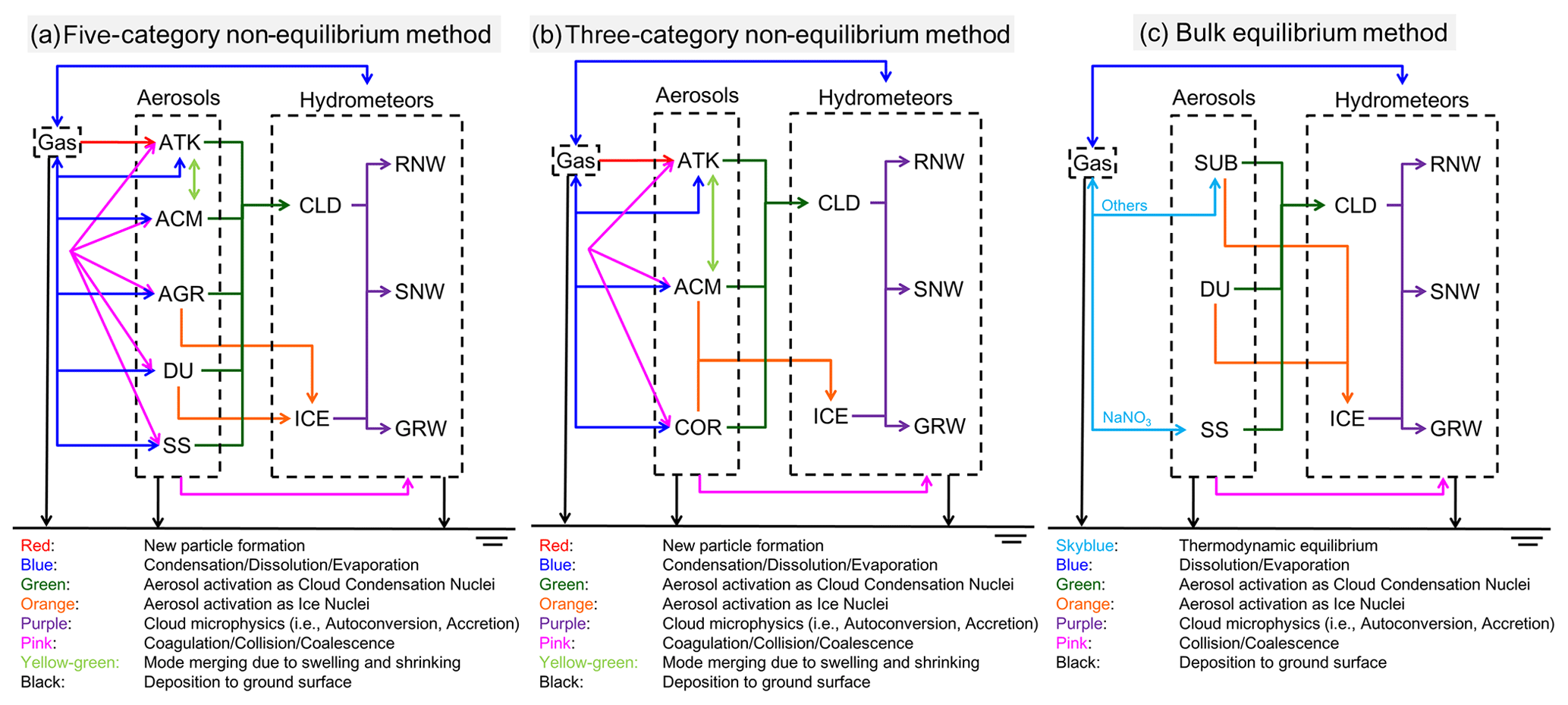
Figure 1Schematic illustrations of gas–aerosol–cloud dynamic processes considered in (a) five-category, (b) three-category (global standard), and (c) bulk equilibrium methods. ATK (Aitken mode), ACM (soot-free accumulation mode, five-category; accumulation mode, three-category), AGR (accumulation mode, mixed with soot aggregate) DU (mixture with dust; both mineral and anthropogenic dust), SS (mixture with sea salt), COR (coarse mode), SUB (submicron), CLD (cloud), ICE (cloud ice), RNW (rain), SNW (snow), and GRW (graupel). This figure is same as Fig. 1 of Kajino et al. (2019a).
Table 1Prognostic variables of aerosol-related attributes.
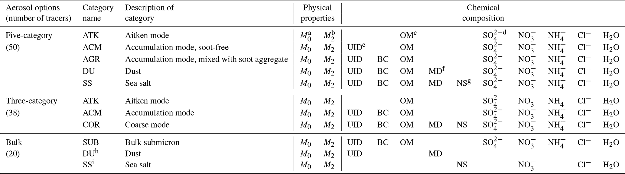
a Zeroth moment, equal to number concentration. b Second moment, proportional to surface area concentration. c Total (primary plus secondary) organic mass, speciation of secondary organics is treated as bulk (gas+aerosol) species. This treatment is feasible under the assumption that the molecular speeds and diffusivities of all organics are the same. d Non-sea-salt only. e Unidentified components, such as anthropogenic dust. f mineral dust mass (natural). g Nonvolatile components of pure sea salt mass (chloride is treated separately as it is volatile). h Assumed to be chemically inert. i Only reacted with HNO3 gas assuming instantaneous thermodynamic equilibrium.
The three-category method (ATK: Aitken mode; ACM: accumulation mode; COR: coarse mode) is a global standard method widely used in regional-scale CTMs, such as WRF-Chem and the Community Multiscale Air Quality (CMAQ) model (WRF-Chem and CMAQ provide other aerosol schemes, such as sectional methods, in addition to the three standard modal methods, e.g., Chapman et al., 2009; Zhang et al., 2004, 2010). These models were originally developed for the purpose of air quality prediction, focusing on factors such as acid deposition, photochemical oxidants, and PM2.5 (Byun and Schere, 2006; Grell et al., 2005); however, they have recently been used to predict the aerosol feedback processes (Chapman et al., 2009; Wong et al., 2012; Kajino et al., 2017). However, the three-category method does not consider the two aspects that are critically important in climate simulations and are thus often resolved by climate models (e.g., Vignati et al., 2004; Pringle et al., 2010; Aquila et al., 2011; Zhang et al., 2012; Liu et al., 2012, 2016): (1) the differences between light-absorbing and non-light-absorbing aerosols and (2) the differences between mineral dust and sea salt particles. To consider these two aspects, the five-category method is implemented by dividing the accumulation mode (ACM of the three-category method) into the ACM (soot-free accumulation mode) and AGR (accumulation mode mixed with soot aggregate) categories and by dividing the coarse mode (COR of the three-category method) into the DU (mixture with dust; i.e., both mineral dust and anthropogenic dust) and SS (mixture with sea salt) categories.
BC is a strong light-absorbing agent and thus alters the climate by heating the air (Bond et al., 2013 and references therein). BC is usually hydrophobic when emitted and externally mixed with other aerosols to become more hygroscopic, forming an internal mixture with other components, including water-soluble inorganics, such as sulfate (), nitrate (), and ammonium (), due to condensation and coagulation during transport (Oshima and Koike, 2013). The in-cloud scavenging of BC, which is the major removal process of BC (Kondo et al., 2011; Oshima et al., 2012), highly depends on the mixing state of BC (Ching et al., 2012; 2016b, 2018). Certainly, the five-category method cannot resolve the mixing state of BC; however, it can simulate the bulk amounts condensed onto BC vs. non-BC particles, whereas the three-category method cannot. Thus, the three-category method will overestimate the condensational growth of BC and therefore overestimate its hygroscopicity, in-cloud scavenging, and subsequent heterogeneous ice nucleation (i.e., immersion freezing). All of the and condense onto BC in the three-category method, although major proportions of and are mixed with non-BC particles in reality (Miyakawa et al., 2014). The degree of overestimation caused by the three-category method relative to the five-category method is presented later in Sect. 6.4.
The three-category method assumes a completely internal mixture of dust and sea salt when the two particles coexist in the same grid box, although the chemical and physical properties of these two particles are very different. In Japan, massive transport events of mineral dust originating from Chinese arid regions, such as the Gobi and Taklimakan deserts, often occur in the spring and are associated with the cold front of migrating anticyclones. Zhang and Iwasaka (2004) found that 10 %–20 % of number fractions of coarse-mode particles were mixtures of mineral dust and sea salt, with similar mass fractions, during dust events in the spring of 1996. They also found only 5 %–15 % of pure dust particles and as much as 60 %–80 % of mixtures of mineral dust and sea salt, including dust mixed with a small amount of sea salt and sea salt mixed with a small amount of dust. Mineral dust is hydrophobic and nonspherical when emitted and thus shows high IN activity, is light absorbing, becomes hygroscopic during transport, and invigorates heterogeneous reactions (Kameda et al., 2016). On the other hand, sea salt is highly hygroscopic and is thus an efficient CCN. The size distributions of mineral dust and sea salt are also very different, so in this three-category method, when the two particles coexist in the same grid box, their combined size distributions and hygroscopicity become unrealistic (i.e., the intermediate values are different from those of both particle types, as shown later in Sect. 6). This three-category representation would be adequate for predicting air pollution over a continent, such as Europe or America. It would also be safe for global climate simulations because, on average, the major global proportions of dust and sea salt exist separately in different locations, namely, over the continents and oceans, respectively. However, for cases of long-range transport over the Asian continent to Japan, mineral dust and anthropogenic pollutants travel in the sea salt-rich boundary layer over the ocean. As discussed in Sect. 6, the three-category method is thus not suitable for air quality and aerosol feedback predictions in East Asia. Consequently, the five-category method is regarded as the standard method of NHM-Chem.
The five-category and three-category methods solve for aerosol microphysical processes by using the triple-moment modal method presented in the previous section (see red, blue, and pink arrows in Fig. 1a and b). Even though a modal approach, which is basically computationally efficient compared to a sectional approach, is used, it is still time consuming because NHM-Chem explicitly models the homogeneous nucleation of sulfuric acid gas to produce 1 nm particles and their subsequent growth due to condensation and coagulation. In terms of the operational forecasts of air quality, such as photochemical oxidants, mineral dust, and PM2.5, the surface mass concentration is of primary importance, and the detailed physical and chemical properties of aerosols are of secondary importance. The operation forecast requires computational efficiency and data assimilation to be applied in order to enhance the predication accuracy rather than solving for detailed physical and chemical processes. For the purpose of obtaining an operational forecast, the computationally efficient bulk equilibrium method is developed, which does not solve aerosol microphysical processes, such as new particle formation, condensation, and coagulation (compare the sky blue arrows in Fig. 1c with the red, blue, and pink arrows in Fig. 1a and b). It should be noted here that the data assimilation was not applied to the simulations, because the current study focused on variations in the model performance due to the different aerosol representations. The same initial and boundary conditions were used for the all simulations. In the bulk equilibrium method, aerosols are categorized into three categories, namely, SUB (submicron), DU (dust), and SS (sea salt). The total dry mass of SUB can be used for the prediction of PM2.5 and the mineral dust mass (denoted as MD) in the DU category can be used for the prediction of dust transport. As mentioned earlier in this subsection, thermodynamic equilibrium is assumed for the inorganic components, and all of the aerosol-phase components are assumed to be categorized into the SUB category, except for NaNO3, which is mixed with sea salt in the SS category. Most of the and exist at the submicron size range, whereas in Japan is usually partitioned into both submicron and supermicron (or coarse-mode) size ranges because the latter is internally mixed with sea salt or mineral dust particles (Kajino et al., 2012b, 2013; Kaneyasu et al., 2012; Uno et al., 2016, 2017). Without considering the coarse-mode , the simulated PM2.5 in East Asia will be significantly overestimated due to the overestimated production of NH4NO3. Certainly, some of the coarse-mode should be mixed with dust, but the DU category is assumed to be inert in the bulk equilibrium method for the purposes of computational efficiency.
As listed in Table 1, the numbers of aerosol attributes for the five-category, three-category, and bulk equilibrium methods are 50, 38, and 20, respectively. In the triple-moment method, the zeroth moment (number) and second moment (proportional to the surface area) are the prognostic (transported) variables, and the third moment (proportional to the volume) is diagnosed based on the mass concentrations of each component and their prescribed densities (i.e., 2.0, 1.77, 2.6, 2.2, 1.83, and 1.0 g cm−3 for UID (unidentified mass, or anthropogenic dust), carbonaceous mass (BC and OM), mineral dust (MD), sea salt (nonvolatile components of sea salt (NS) and Cl−), inorganics (, , and ), and water (H2O), respectively). Here, note that the NS indicates the nonvolatile mass of pure sea salt particles, namely, the dry sea salt mass minus the Cl− mass.
The rules for the transfer of moments and mass from one category to another due to intercategory coagulation and mode merging are listed in Table 2. The intercategory coagulation rules of “from smaller to larger category” are used for the three-category and five-category methods; additionally, the coagulation rules of “from hydrophobic to hygroscopic category” and “from non-light-absorbing to light-absorbing category” are used for the five-category method. The mode merging represents the transfer of moments and mass greater than the threshold diameter of 40 nm due to condensation or self-coagulation growth. During its emission, the UID only exists in ACM and DU in the five-category method, in ACM and COR in the three-category method, and in SUB and DU in the bulk method. Due to intercategory coagulation, the UID is also found in AGR and SS in the five-category method. Freshly emitted BC only exists in AGR, ACM, and SUB in the five-category, three-category, and bulk methods, respectively. The intercategory coagulation transfers BC to the DU and SS categories in the five-category method and to COR in the three-category method. OM exists in ATK, ACM, and AGR in the five-category method, in ATK and ACM in the three-category method, and in the SUB category in the bulk method during its emission. OM is moved to the DU and SS categories in the five-category method and to the COR category in the three-category method. The MD mass only exists in the DU category for the five-category and bulk methods, and it exists in the COR for the three-category method. Transfer of the MD mass to the SS category is predicted only with the five-category method. All of the secondary and semivolatile components, such as OM, , , , and Cl−, can exist in all of the categories in the five-category and three-category methods. They can exist only in SUB in the bulk method, except for and Cl−, which can mix with sea salt, as mentioned earlier (Cl− also exists in the SS category during emission). All of the aerosol categories can be hygroscopic and thus contain H2O, except for the DU category of the bulk method. As mentioned earlier, crustal cations play an essential role in fixing acidic gases to the aerosol phase. In all three methods, the composition of the sea salt and dust particles is defined after Song and Carmichael (2001) as follows: the MD mass contains 6.8, 1.6, 0.91, and 0.78 wt % Ca2+, Na+, K+, and Mg2+, respectively, and the NS mass contains 68.1, 17.1, 8.21, 2.58, and 2.45 wt % Na+, , Mg2+, Ca2+, and K+, respectively. It is assumed that the UID mass does not contain any cations and is thus hydrophobic and inert.
Table 2Rules for the transfer of moments and chemical mass concentrations from one category to another due to intercategory coagulation and mode merging.
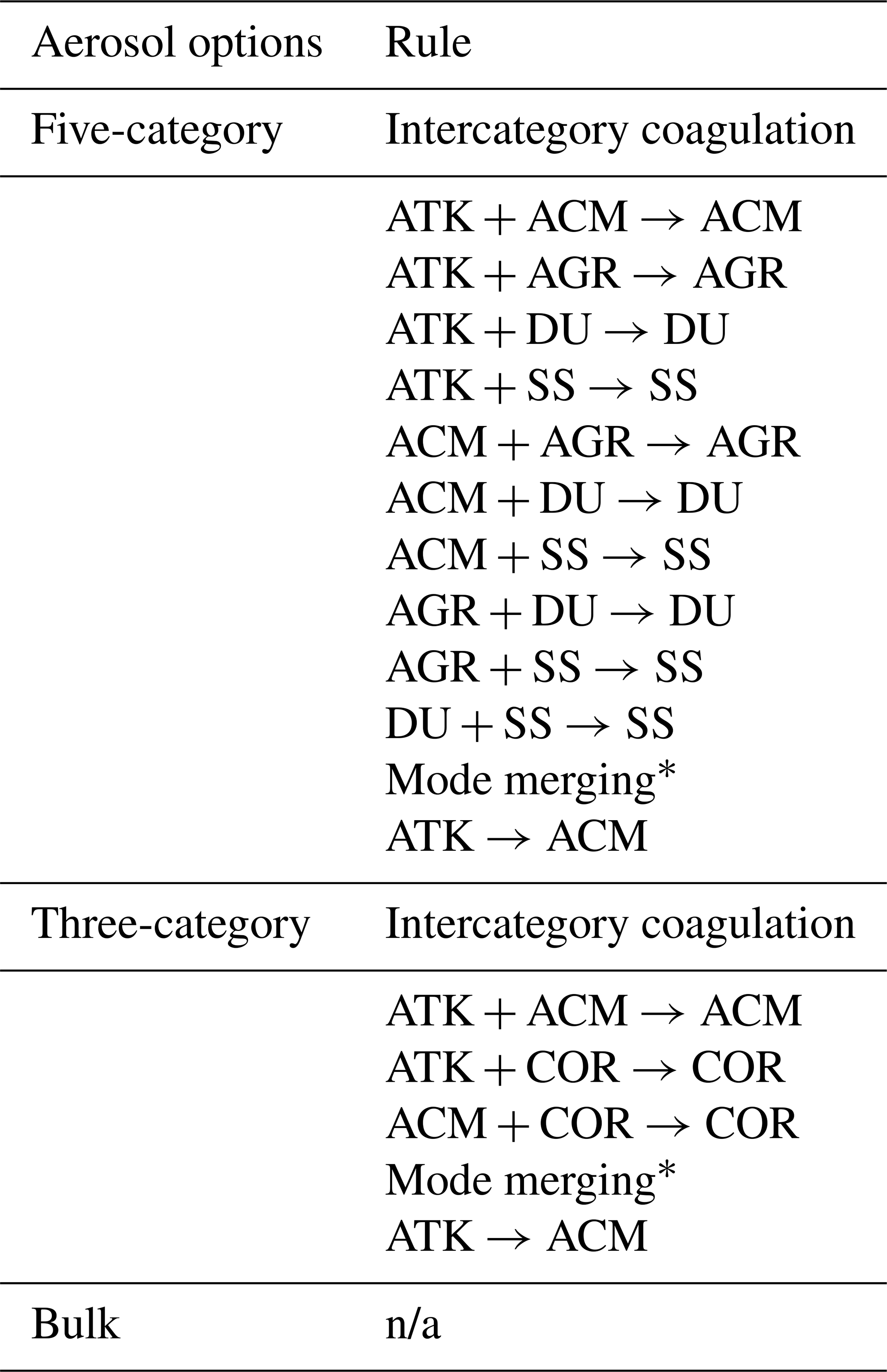
* Transfer of moments and mass greater than 40 nm due to condensation or self-coagulation growth. n/a – not applicable
In terms of aerosol water uptake, non-equilibrium treatment is critically important, especially for higher relative humidity conditions and coarse-mode particles, because the instantaneous equilibrium assumption can cause unrealistic overestimates of aerosol diameter. For example, the equilibrium diameter of an aerosol with a dry diameter of 1.0 µm and a hygroscopicity κ value of 1.0 reaches 21.2 µm at a relative humidity RH=100 % (see the κ-Köhler theory; Petters and Kreidenweis, 2007), which is equal to or greater than the initial sizes of cloud droplets. Under actual atmospheric conditions, aerosols cannot reach such a large equilibrium diameter, either because it takes too long to reach (for low aerosol populations) or because aerosols remove too much water vapor from the air, such that the relative humidity becomes substantially lower (for high-enough aerosol populations). Therefore, in the three-category and five-category non-equilibrium methods, aerosol water uptake is also calculated in a non-equilibrium manner: the mass transfer of water vapor is driven by the differences between the current water content and equilibrium water content, which is derived using the Zdanovskii–Stokes–Robinson (ZSR) method (Fountoukis and Nenes, 2007). Note that the RH of air is assumed to remain unchanged due to water uptake by aerosols. In the bulk equilibrium method, instantaneous equilibrium is assumed for the aerosol water content, but a maximum threshold of an ambient RH of 98 % is used to avoid the abovementioned unrealistically large aerosol size.
4.1 Model domain, simulation period, and boundary conditions
The simulation settings such as the model domain and boundary conditions used in this study are presented in this section. They were the same as Kajino et al. (2019a) and thus are briefly described in this section; detailed descriptions, especially of the aerosols, are provided in Sect. 4.2. Figure 2 shows a flowchart of the simulations, including the simulation domain, which covers East Asia with 200×140 horizontal grid cells with a grid resolution of Δx=30 km. The numbers of vertical grid cells in the NHM and CTM are 38 (reaching up to 22 055 m a.s.l.) and 40 (reaching up to 18 000 m a.s.l.), respectively, with terrain-following coordinates. The input/output time interval of the offline coupled NHM-Chem was 1 h. The analysis period was the entire year of 2006, but two half-year CTM simulations were conducted and then combined due to the initialization issue regarding the land surface model. Climatological data were used for the initial condition of the land surface model (Simple Biosphere Model; SiB) of the NHM. If the simulation started in winter, the initial climatological snow coverage could be very different from that at the actual simulation time; thus, a longer spin-up period would be required. To avoid this situation, July was selected as the initial simulation time because over a year, July corresponds to the minimum snow coverage over East Asia. Therefore, two NHM simulations were performed: from July 2005 to June 2006 and from July to December 2006 with a spin-up period of 5 d. Then, the two CTM simulations were conducted from January to June 2006 and from July to December 2006 with the 5 d spin-up and used in the following analysis.
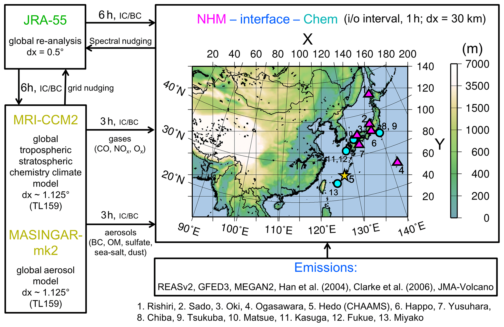
Figure 2Current simulation settings, model domain showing terrestrial elevation (m), and observation sites. The pink triangles numbered 1–7 show the Japanese EANET sites, except site 5. Hedo (CHAAMS) is marked as the yellow star, where the SKYNET and AD-Net Hedo sites are located on the same premises. The blue circles numbered 8–13 indicate the SKYNET or AD-Net sites in Japan.
The 6-hourly global Japanese 55-year Reanalysis (JRA-55) (Kobayashi et al., 2015) data were used to set the initial and boundary conditions of the NHM. Spectral nudging was applied to constrain the simulated meteorological field toward the global analysis, above a height of 7 km for large-scale wave components (wavelength>1000 km) of horizontal momentum and potential temperature, with a weighting factor of 0.06 (Nakano et al., 2012). Data assimilation was not applied to the chemical fields in this study.
The 3-hourly lateral and upper boundary concentrations of gases and aerosols were obtained from the simulation results of the global models of the Meteorological Research Institute Chemistry-Climate Model version 2 (MRI-CCM2) (Deushi and Shibata, 2011) (TL159, ) and the Model of Aerosol Species in the Global Atmosphere mark-2 (MASINGAR mk-2) (Tanaka et al., 2003; Tanaka and Ogi, 2017; Yumimoto et al., 2017) (TL159, ), respectively. Because the lumped mechanisms of non-methane volatile organic compounds (NMVOCs) and aerosol representations of NHM-Chem are different from those of the two global models, only NOx, O3, and CO were taken from the MRI-CCM2 (in other words, the lateral boundaries should be far enough that the peroxyacetyl nitrate (PAN) and long-lived NMVOC fluxes from the boundaries are less influential on the concentrations over the targeted sites of the simulation), and the total masses of BC, organic carbon (OC), , mineral dust, and sea salt were taken from MASINGAR mk-2 (although this model employs sectional methods for mineral dust and sea salt). An OM-to-OC ratio of 1.8 and a 100 % existence of as (NH4)2SO4 were assumed in the boundary concentrations. The mineral dust and sea salt were treated as being externally mixed, whereas all of the BC, OM, and (NH4)2SO4 were included in the ACM in the three-category method and in the SUB category in the bulk equilibrium method. For the five-category method, we assumed that 80 % of the BC, OM, and (NH4)2SO4 were attributed to ACM and that the other aerosols were attributed to AGR.
4.2 Emission datasets
We used the Regional Emission inventory in ASia version 2 (REASv2) (Kurokawa et al., 2013) with a resolution for the anthropogenic emissions of NOx, SO2, NH3, NMVOC, BC, primary organic carbon (POC), PM2.5 and PM10 with monthly variations. There is no monthly variation in NH3. Because REASv2 does not provide hourly and vertical profiles of emissions, those of Li et al. (2017) were applied to each sector, i.e., power, industry, domestic, transport, aviation, and large point sources. We used the monthly Global Fire Emissions Database (GFED3; Giglio et al., 2010) with a resolution for open biomass burning emissions (NOx, SO2, NMVOCs, BC, and POC) and the Model of Emissions of Gases and Aerosols from Nature (MEGAN2; Guenther et al., 2006) for biogenic emissions of isoprene, terpenes, methanol, and NO. We applied the monthly mean values of GFED3 without daily and diurnal variations. The temporally varying biogenic emission flux was calculated by Eq. (1) of Guenther et al. (2006) using the surface solar radiation and surface air temperature, as simulated by NHM. Biogenic emissions were allocated to the bottom layer. The open biomass burning emissions were uniformly allocated from the bottom layer up to 1000 m a.g.l. The lightning NOx emission was not considered in the current simulation.
We made the following assumptions for the ratios of lumped species in the anthropogenic and biomass burning emissions. REASv2 provided speciation information about NMVOC, which was redistributed to the NMVOC speciation of the Statewide Air Pollution Research Center, version 1999 (SAPRC-99) chemical mechanism. Because GFEDv3 does not provide NMVOC speciation information, that of Woo et al. (2003) was applied and allocated to the SAPRC-99 speciation. When a SAPRC-99 speciation was finer than that of REASv2 or GFEDv3, the speciated NMVOC of REASv2 or GFEDv3 was equally distributed to that of SAPRC-99 with equal mixing ratios. The OM-to-OC ratio was set to 1.8 for both emissions. The NOx emissions were partitioned as 90 % NO and 10 % NO2. Overall, 5 % of SO2 emissions were regarded as . The UID emissions of the fine and coarse modes were defined as PM2.5 minus the BC minus the POM (primary organic mass; 1.8×POC) and PM10 minus PM2.5, respectively. The emissions were partitioned as 10 % ATK and 90 % ACM for the five-category and three-category methods. Of the POM emissions, 5 %, 10 %, and 85 % were distributed to ATK, AGR, and ACM in the five-category method, whereas 5 % and 95 % of these emissions were distributed to ATK and ACM in the three-category method, respectively.
Hourly volcanic SO2 emissions in Japan were developed in this study. These emissions were assumed to comprise 100 % SO2, and no volcanic emissions were considered. JMA regularly monitors the SO2 emission fluxes and smoke heights of the six major volcanoes in Japan. Since the observation data are sporadic over time and the observation frequencies vary depending on the volcanoes and periods considered, cubic spline interpolation was applied over time to obtain hourly data, as done by Kajino et al. (2004). The details of this approach are described in Supplement 2.
The methods of Han et al. (2004) and Clarke et al. (2006) were used to predict the emissions of mineral dust and sea salt particles as functions of the friction velocity and 10 m wind speed, respectively. In addition to the formula of Han et al. (2004), simulated snow coverage was applied to reduce the emission flux. Flux adjustments were made for the mineral dust and sea salt emissions by using the observed non-sea-salt (nss) Ca2+ (defined as (µg m−2 or µg m−3)) and PM10 values for the mineral dust and the observed Na+ and PM10 values for the sea salt obtained at the seven Japanese Acid Deposition Monitoring Network in East Asia (EANET) stations. The adjustment ratios of the dust and sea salt emission fluxes in the simulations were 0.5 and 0.3, respectively.
4.3 Aerosol size parameters in emission and boundary conditions
The symbols used for the aerosol parameters used in this study are summarized in Table 3. Aerosol sizes should be carefully defined because both their physical and optical measures significantly vary depending on whether their diameters are number equivalent or mass equivalent, wet or dry, and actual or aerodynamic. The width of the distribution σg, hygroscopicity κ, and aerosol density ρp are also key parameters because they affect the magnitudes of their physical and optical measures. Certainly, shape factors can also significantly affect these measures, as well as aerosol microphysical processes; however, all of the modeled particles are assumed to be spherical in the current version of NHM-Chem, as they are in most other CTMs.
Table 3Symbols used for aerosol size parameters and their relationships.
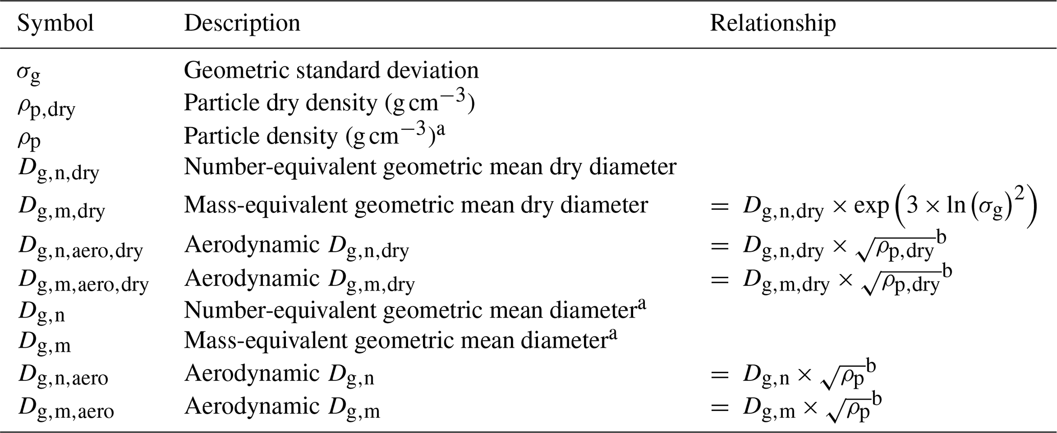
a When wet or ambient. b For spheres.
Both Han et al. (2004) and Clarke et al. (2006) provided size-resolved emission fluxes, whereas this model assumes a log-normal size distribution. The values of the number equivalent dry of the mineral dust and sea salt emissions were obtained by assuming the prescribed σg as 2.0. The values of the mineral dust were 0.66, 1.22, and 1.22 µm for the land use category (LUC) of desert, loess, and grass, respectively. For a reference, values of 0.66 and 1.22 µm correspond to aerodynamic values of 1.06 and 1.96 µm, mass-equivalent dry aerodynamic values of 4.50 and 8.31 µm, and ratios of 0.23 and 0.068, respectively. Note that here, the simulated PMx was derived as a proportion of the dry mass in which the aerodynamic ambient (wet) diameter was smaller than x µm.
The simulated PMx was calculated using the error function (erf) as follows:
where i and Mi indicate the category and dry mass of the category, respectively.
We made the following assumptions for the aerosol size distributions at the boundary conditions. Because Clarke et al. (2006) proposed trimodal size distributions, they needed to be combined into a single mode. Laboratory and field experiments indicated that the major proportions of the smallest mode (i.e., 10–132 nm) should be water-insoluble organic compounds (Facchini et al., 2008; Prather et al., 2013); thus, the smallest mode was not regarded as sea salt emissions in this model. The number and volume fluxes of the sea salt emission were obtained as the summations of those of the second-largest and largest modes. The surface area flux was then deduced based on the number, volume, and prescribed value of σg=2.0. The value, value, and ratio of the dry sea salt particles are 0.448, 1.89, and 0.66 µm, respectively. Because sea salt particles are highly hygroscopic, at conditions of RH=80 % and 90 %, the ambient diameter values would be 2.39 and 2.88 µm, and the ratios would be 0.54 and 0.44, respectively, assuming a hygroscopicity value of κ=1.0.
The prescribed size parameters were applied to the emissions of all of the species, except for the mineral dust and sea salt and are defined as follows: (, , (0.1 µm,1.5), (0.1 µm,1.5), and (2 µm,1.8) for the ATK, ACM, AGR, and DU (applied to anthropogenic dust only, denoted as UID) categories of the five-category method; (0.01 µm,1.3), (0.1 µm,1.5), and (2 µm,1.8) for the ATK, ACM, and COR (applied to UID only) categories of the three-category method; and (0.1 µm,1.5) and (2 µm,1.8) for the SUB and DU (applied to UID only) categories of the bulk equilibrium method, respectively.
Although MASINGAR mk-2 employs a sectional model to predict changes in aerosol size distributions, the prescribed size parameters were applied to the lateral and upper boundary concentrations of NHM-Chem and are defined as follows: (, , (0.1 µm,1.5), (0.1 µm,1.5), (2 µm,1.8), and (1 µm,1.8) for the ATK, ACM, AGR, DU, and SS categories of the five-category method; (0.01 µm,1.3), (0.1 µm,1.5), and (1 µm,1.8) for the ATK, ACM, and COR (mineral dust and sea salt) categories of the three-category method; and (0.1 µm,1.5), (2 µm,1.8), and (1 µm,1.8) for the SUB, DU, and SS categories of the bulk method, respectively. Certainly, in the self-nesting simulations, where the boundary concentrations are taken from the outer domain simulation of NHM-Chem, the prescribed size parameters are not needed.
The observation data used for the evaluations of the simulation results are described in this section.
The observation sites used for the model validation are depicted in Fig. 2. The pink triangles indicate the Acid Deposition Monitoring Network in East Asia (EANET) stations (http://www.eanet.asia, last access: 18 June 2020). The blue circles indicate the ground-based international remote sensing network dedicated to aerosol–cloud–radiation interaction studies (SKYNET) stations (Takamura et al., 2004; Nakajima et al., 2007; http://atmos3.cr.chiba-u.jp/skynet, last access: 18 June 2020) and/or the Asian dust and aerosol lidar observation network (AD-Net) stations (Sugimoto et al., 2008; Shimizu et al., 2016; http://www-lidar.nies.go.jp/AD-Net/, last access: 18 June 2020). At the Japanese EANET sites, the hourly surface concentrations of gases (NOx, SO2, and O3) and the aerosol mass (PM2.5 (only Oki and Rishiri for 2006) and PM10), daily wet depositions of inorganic compounds, and 2- or 1-week mean concentrations of gaseous and aerosol phases of inorganic compounds are monitored. At the SKYNET sites, sky radiometers (Prede Co. Ltd., Tokyo, Japan) are the main instruments. Aerosol optical thickness (AOT) and single scattering albedo (SSA) data in ultraviolet–visible–near-infrared regions and the Ångström exponent data are provided. We used AOT and SSA at 500 nm for the comparison. The AD-Net sites are equipped with a two-wavelength (1064 and 532 nm) polarization-sensitive (532 nm) Mie-scattering lidar system. We used the extinction coefficients for non-spherical (referred to as dust) and spherical aerosols for the model evaluation, derived using the attenuated backscattering coefficients and the volume depolarization ratio (Sugimoto et al., 2003; Shimizu et al., 2004). The yellow star indicates the Hedo site, which belongs to both EANET and SKYNET, an air quality measurement supersite called CHAAMS (Cape Hedo Atmosphere and Aerosol Monitoring Station).
The optical particle counter (OPC) (ROYCO LAS236) was equipped at CHAAMS in 2006, which measures number concentrations of aerosols with diameters larger than 0.3, 0.5, 1, 3, and 5 µm (Takamura et al., 2004). To compare the simulated number concentrations against the OPC data, a parameter NCx is defined, the proportion of the number concentration for which the aerodynamic ambient diameter is larger than x µm, as follows:
where i and Ni indicate the category and total number of the category, respectively. The simulated NC0.3 was compared against that observed by OPC.
Because aerosol optical properties are not simulated in NHM-Chem, to compare with the observation data, the Mie theory calculation was performed by using simulated log-normal size distribution parameters and chemical composition. The refractive indices of the Optical Properties of Aerosols and Clouds (OPAC) database (Hess et al., 1998) were used for the Mie calculation. For the refractive indices of the model components of UID, BC, OM, MD, NS, , , , Cl−, and H2O, the databases of “insoluble”, “soot”, “insoluble”, “mineral”, “sea salt”, “water-soluble”, “water-soluble”, “water-soluble”, “sea salt”, and “fog” values, respectively, were used, with some modifications for BC to 1.85−0.71i (Bond et al., 2006) and MD to 1.5−0.001i (Aoki et al., 2005) at 500 nm. To calculate the optical properties of non-light-absorbing and light-absorbing mixtures, the Maxwell Garnett approximation was used. The BC and MD masses were regarded as light-absorbing components, and the others were regarded as non-light-absorbing (certainly, some proportions of OM are light-absorbing, i.e., brown carbon, but they are not considered in the current model). The volume-weighted refractive indices were used for the light-absorbing and non-light-absorbing components in each category.
In the current study, a model performance comparison of the aerosol representation methods was made in terms of the computational costs (Sect. 6.1), the mass concentrations of O3, mineral dust and PM2.5 (Sect. 6.2), the deposition of inorganics such as , , and (Sect. 6.3), AOT and light-absorbing AOT (AAOT) (Sect. 6.4), and CCN (Sect. 6.5). In Table 4, the statistical measures listed are the median of simulation data (sim. med.) and simulation to observation median ratio (sim : obs), correlation coefficient (R), and fractions of simulated values within a factor of 2 of the observed values (Fa2) of the relevant variables such as O3 and its precursor gas NOx, dust extinction coefficient (Ext_D) and PM10 during the dust events of April 2006 (defined as PM10_D, later in Sect. 6.2), PM2.5, wet deposition amounts of , , and , AOT, SSA, total (dust and spherical) extinction coefficient (Ext_T), and NC0.3. Because the main objective of the paper is the aerosol module intercomparison, the general description of the results, which was already done in our previous paper (Kajino et al., 2019a), is not presented in detail here but is presented in Supplement 3.
Table 4Comparative statistical analysis of observed (obs.) and simulated (sim.) variables. Here, “5-ctg” and “3-ctg” indicate the five-category and three-category methods, respectively, and “blk” indicates the bulk method.
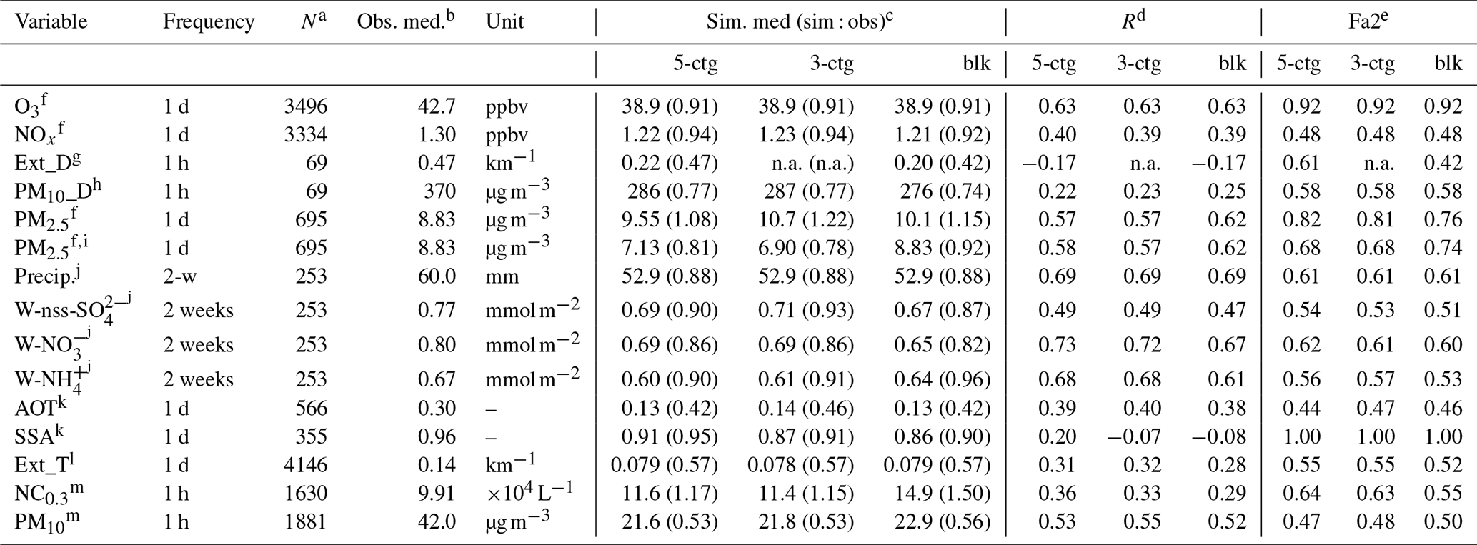
a Number of available data. b Median of observation data. c Median of simulation data and simulation to observation median ratio with brackets. d Correlation coefficient. e Fraction of simulated values within a factor of 2 of the observed values. f Daily mean surface concentration. g Hourly mean median values below 300 m of extinction coefficient during the dust events in April 2006 at Matsue and Hedo. h Hourly mean values during the dust events in April 2006 at Oki and Hedo. i PM2.5 but compared with simulated PM2.5 (pile-up). j Half-monthly cumulative precipitation or wet deposition amount. k Daily mean column amount. l Daily mean median values below 300 m of extinction coefficient. m Hourly mean surface concentration in April and December 2006 when the OPC data are available at Hedo.
In this section, the intermodule comparisons between the bulk equilibrium, three-category, and five-category methods are presented in terms of their relevant purposes, i.e., simulations of variables often used for operational forecast (such as O3, mineral dust, and PM2.5), simulations of air quality variables (surface concentrations and depositions of pollutants), and simulations of climate-relevant variables (such as AOT, CCN, and ice-nucleating particles (INPs)), respectively.
It should be noted here that the capability of the bulk equilibrium method in terms of operational forecast was not assessed by conducting forecast simulations (e.g., 3 d forecast with a data assimilation of initial conditions and post-processing for statistical bias corrections) but assessed in the hindcast simulation without data assimilations and post-processing.
The main objectives of this section are itemized as follows: (1) to compare the computational efficiency of the three methods, (2) to quantify the deviations of the widely used three-category method and the efficient bulk equilibrium method from the most realistic aerosol representation of NHM-Chem, the five-category method, and (3) to assess the discrepancy between the simulated and observed variables and how the discrepancy varied depending on the three methods.
6.1 Computational costs
The computational costs of the three methods are listed in Table 5. RCPUtime and Raero were measured for the earlier half-year simulations (i.e., January to June 2006). The non-equilibrium aerosol microphysics module consumed approximately half of the total CPU time for the five-category method, while it consumed only 15 % of that of the bulk equilibrium module (and the thermodynamic equilibrium model ISORROPIA2 consumed a major proportion of this 15 %). The total CPU times of the three-category and five-category methods are 44 % and 91 % greater than that of the bulk equilibrium module, respectively. For these three options, the number of gaseous species is the same (58), and the number of their aerosol attributes is 20, 38, and 50, respectively.
Table 5Number of transport variables (gas plus aerosol attributes) (Ntrans) and ratios of the total CPU time to that of the bulk chemistry (RCPUtime), as well as ratios of CPU time of the aerosol process to that of the total processes1 (Raero).
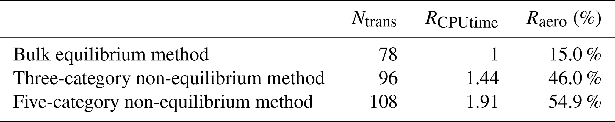
1 Excluding the I/O and MPI communications.
6.2 Surface mass concentration of air pollutants
Figures 3–5 present the seasonal mean surface mass concentrations of O3, mineral dust, and PM2.5, which negatively impact the health of the population and the environment and thus are often used in operational air quality forecasts. The comparisons between the simulated and observed variables are summarized in Supplement 3 and Figs. S3-1–S3.3 in the Supplement, respectively.
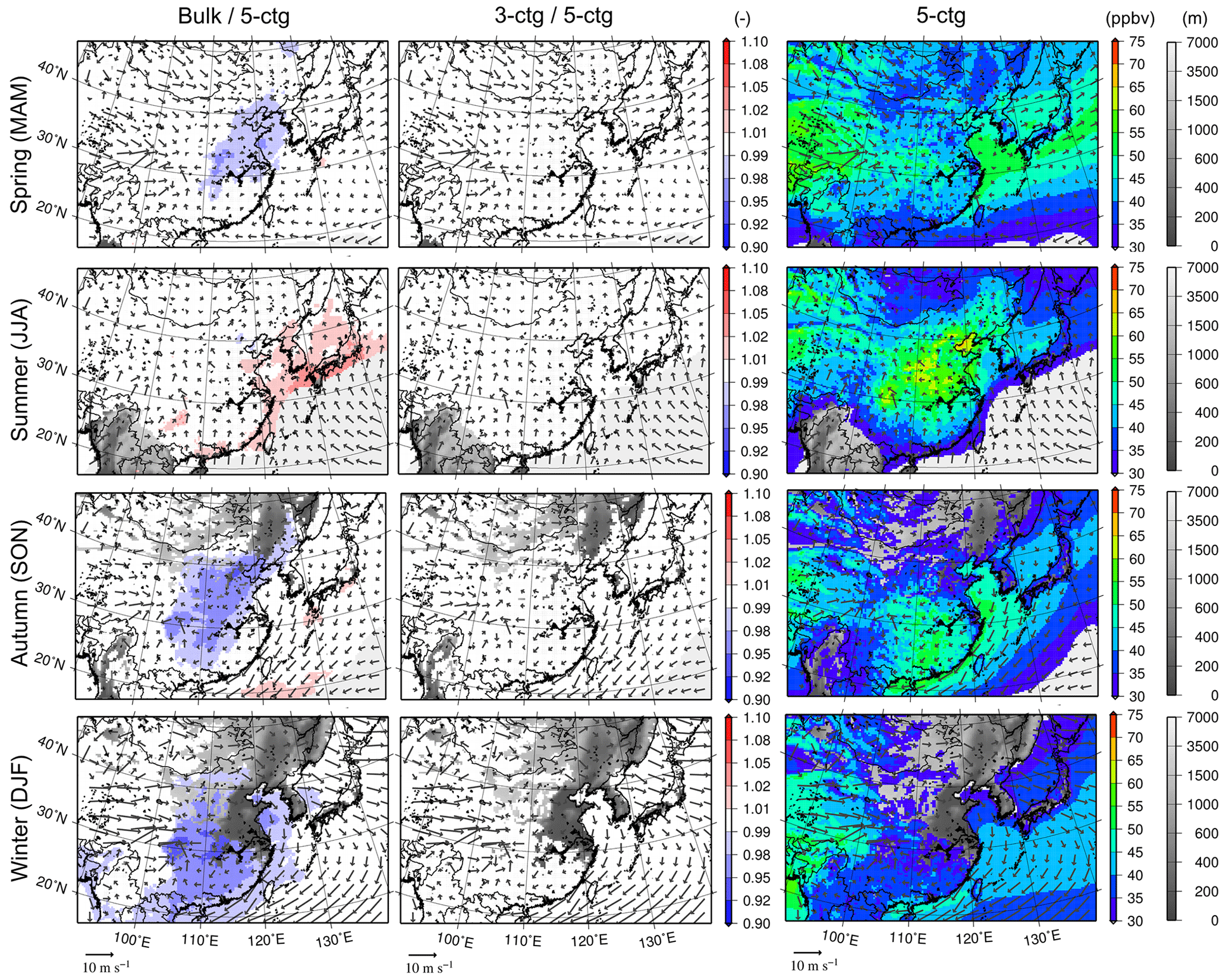
Figure 3Seasonal mean surface concentrations of O3 in (top to bottom) spring, summer, autumn, and winter of 2006 for (left to right) the ratios of the bulk to five-category methods, the ratios of the three-category to five-category methods, and the five-category method with surface wind vectors. The model topography is depicted in grayscale on the background of each panel. Topography is overlain by color shades for concentrations above the lower limit of the scale (in this case, 30 ppbv).
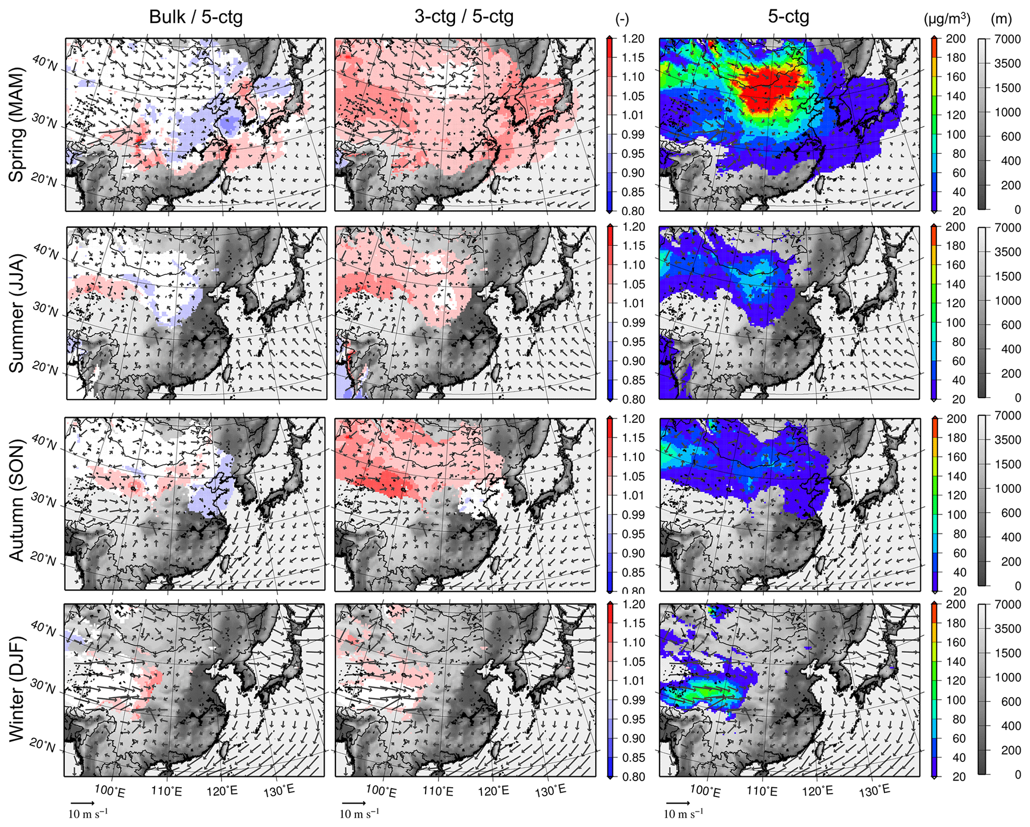
Figure 4Same as Fig. 3 but for mineral dust.
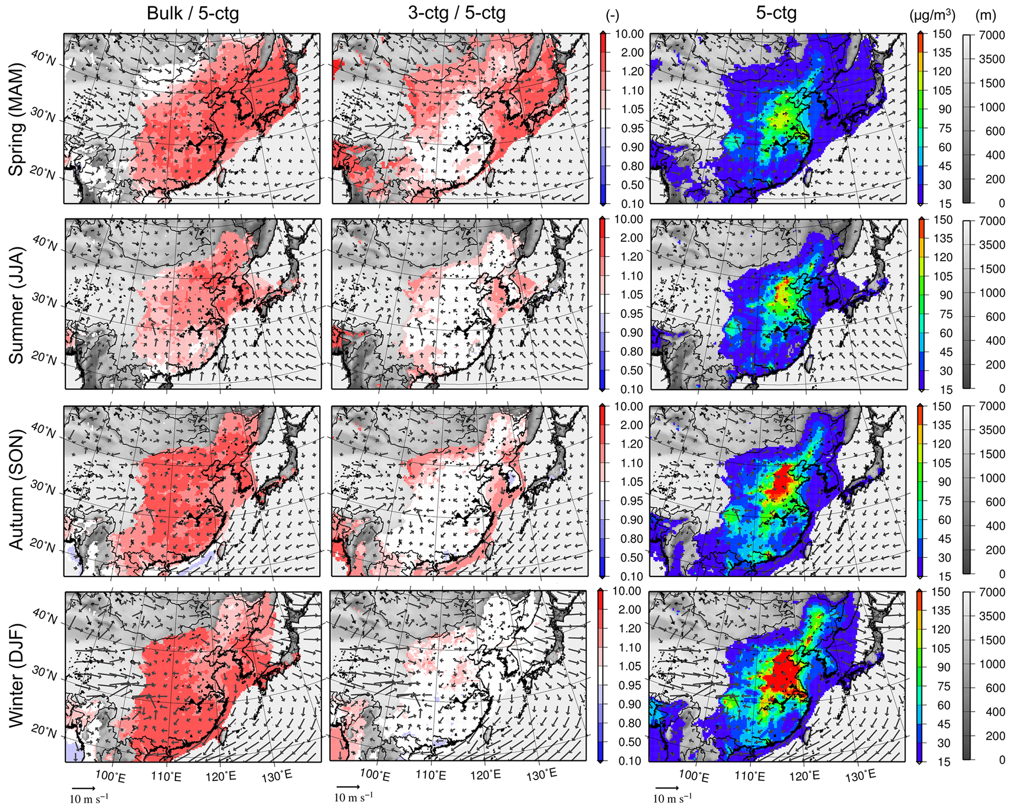
Figure 5Same as Figs. 3 and 4 but for PM2.5.
The midlatitude westerlies are predominant in this region, and air pollutants are transported from west (or northwest) to east (or southeast), associated with migrating disturbances, including the cold and warm frontal transport of cyclones and anticyclonic transport throughout the year except during summer (e.g., Oshima et al., 2013). In summer, due to the Pacific High system, the transport of continental air masses is less dominant, and clean air masses of maritime origin are often transported to Japan. Northerly to northwesterly winds prevail in winter due to the Siberian High system. These seasonal wind patterns can be clearly observed in Figs. 3–5.
The difference in the horizontal distributions of O3 between the bulk method and the other two methods was very small (Fig. 3). The differences between the bulk O3 and five-category O3 were due mainly to the differences in the aerosol surface areas (different heterogeneous loss rates of NOx, as a precursor of O3 formation). It is inferred from Table 4 that the relative magnitudes of sim : obs of NOx and O3 of the three methods are consistent (sim : obs of NOx of the bulk, three-category, and five-category methods were 0.925, 0.939, and 0.938, and those of O3 were 0.9108, 0.9115, and 0.9111, respectively). Further investigation is needed for quantitative assessment, but the errors of the bulk method were smaller than those of the other methods considered by up to 5 %. Because this difference is minor compared to the difference between the simulation and observation results (especially for R), improving the model processes and/or boundary conditions will certainly improve all of the simulation results, regardless of the aerosol category methods that are selected.
The simulated surface mineral dust concentration was highest in the spring in the emission source regions (Taklamakan and Gobi) and the downwind regions such as Korea and Japan (Fig. 4). The differences between the bulk and five-category methods were generally lower than 5 % and at most 10 % (Fig. 4). These differences could be due mainly to the differences in the chemical aging of the mineral dust, which increases in hygroscopicity due to condensational growth during its long-range transport in the five-category method. There are even more significant differences found between the three-category and five-category methods. The three-category and five-category methods both consider chemical aging processes, but the three-category method assumes a complete internal mixture of dust and sea salt. Accordingly, the dust particles were more hygroscopic but smaller in the three-category method compared to those in the five-category method case; thus, with the three-category method, the surface concentration was higher over the ocean in the spring by up to 10 % due to the lower gravitational and dry deposition velocities. The three-category to five-category dust concentration ratio was higher in the regions on the continent close to the west lateral boundary due to the difference in the dust sizes; additionally, a complete dust/sea salt mixture was assumed at the boundary in the three-category method. Because this difference (up to 10 %) is minor compared to the difference between the simulation and observation (approximately 0.4–0.6 of Fa2; see Table 4), improving the model processes and/or boundary conditions will certainly improve all of the simulation results regardless of the aerosol category methods that are selected.
The differences in the model performance of the PM2.5 prediction are shown in Fig. 5. This PM2.5 was derived by Eq. (1), but the simulated PM2.5 was sometimes defined as the pile-up of the mass concentrations of the dry components existing in the submicron categories, which is independent from the aerosol size distribution. The latter is denoted as PM2.5 (pile-up) in the paper, and the horizontal distributions are shown in Fig. S4-1 in Supplement 4. The major difference between the simulated PM2.5 and PM2.5 (pile-up) is that PM2.5 includes some proportion of natural aerosols, such as sea salt and dust, and can exclude proportions of submicron categories (i.e., ACM and AGR) larger than 2.5 µm, whereas PM2.5 (pile-up) completely excludes sea salt and dust particles and includes all of the submicron categories (i.e., ATK, ACM and AGR in the five-category method, ATK and ACM in the three-category method, and SUB in the bulk method). The simulated PM2.5 concentration over China was highest in the spring (Fig. 5). PM2.5 and PM2.5 (pile-up) of the bulk method were 20 %–100 % larger than those of the five-category and three-category methods due to the neglection of nitrate mixed with coarse-mode dust particles by the bulk method. In the five-category and three-category models or in reality, nitrate is mixed with mineral dust particles forming Ca(NO3)2 and Mg(NO3)2 and with anthropogenic dust by condensation of NH4NO3. The simulated submicron and supermicron were comparable in the five-category and three-category methods over the continent for the whole seasons and over the ocean in the spring. However, all of these supermicron values were mixed with SUB in the bulk method, which caused significant overestimation of both PM2.5 and PM2.5 (pile-up). The overestimation was predominant in the colder seasons over the continent, because the particulate phase of is larger as the temperature is lower. PM2.5 of the three-category method were 20 %–100 % larger than those of the five-category method especially over the ocean in the spring. It is due to the unrealistic complete internal mixing assumption of the sea salt and dust particles in the three-category method. The sea salt and dust particles coexisted mostly as external mixtures over the ocean in the spring. As the size of sea salt is generally smaller than that of dust, mass fractions of sea salt (SS of five-category method) smaller than 2.5 µm are larger than those of dust (DU of five-category method). However, the internal mixing assumptions resulted in smaller size of COR than DU, which resulted in overestimation of mass fractions of DU smaller than 2.5 µm and thus overestimation of PM2.5 by the three-category method. In contrast, the three-category to five-category ratio of PM2.5 (pile-up) was negligibly small, indicating that the internal sea salt–dust mixture assumption has a minor impact of the dry mass concentrations of the submicron categories. Despite the non-negligible differences in the predicted surface concentrations of PM2.5 and PM2.5 (pile-up) by the three methods, the statistical scores for the three methods are not different from one another (Table 4). It is indicated that the bulk method is eligible for operational forecasting, because the computational efficiency does not significantly deteriorate the model performance in terms of the predictions of PM2.5 surface concentrations.
6.3 Dry, wet, and fog deposition of acidic substances
Figures 6 and 7 compare the predictions of the dry and wet depositions of the inorganic components of non-sea-salt (nss-, defined as (µg m−2 or µg m−3)), total (gas plus aerosol) (T-), and T-, which are the major acidic and basic substances, obtained using the three methods. Once deposited on the ground surface, is efficiently converted to in the soil; thus, is also an important agent for environmental acidification. The horizontal distribution of dry deposition was generally similar to that of surface concentration because the dry deposition flux is proportional to the surface concentration.
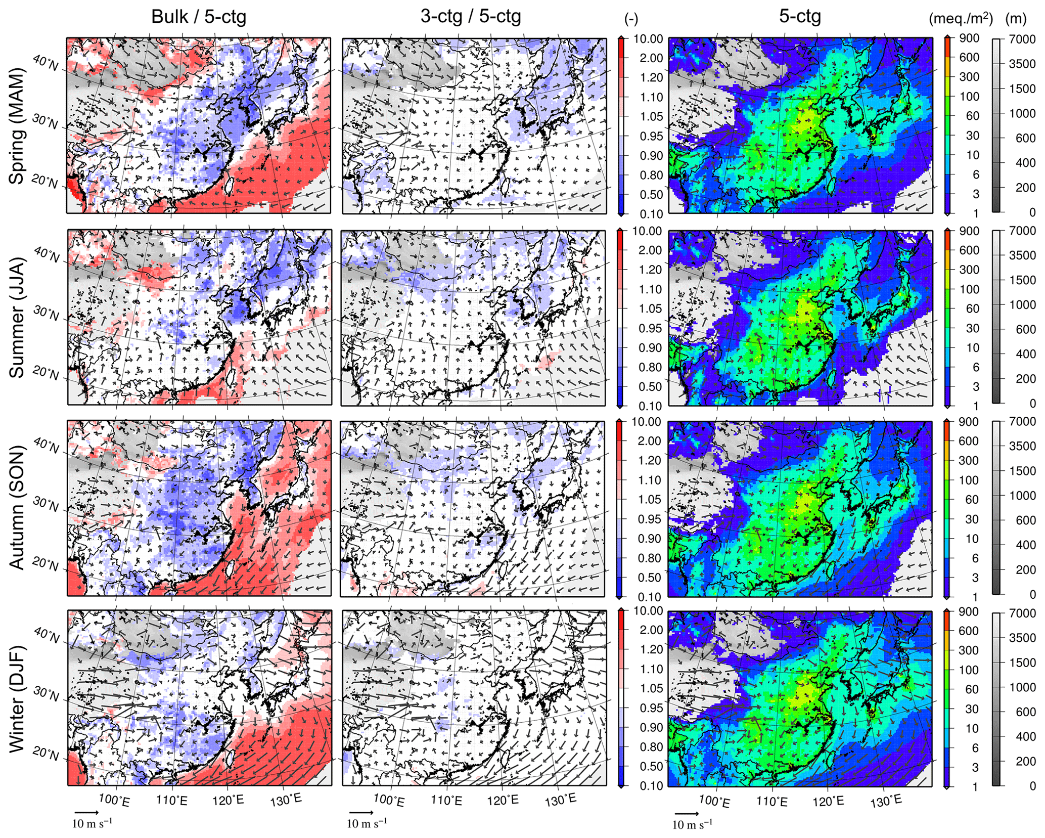
Figure 6Same as Figs. 3–5 but for the dry deposition of sum of nss-, T-, and T-.
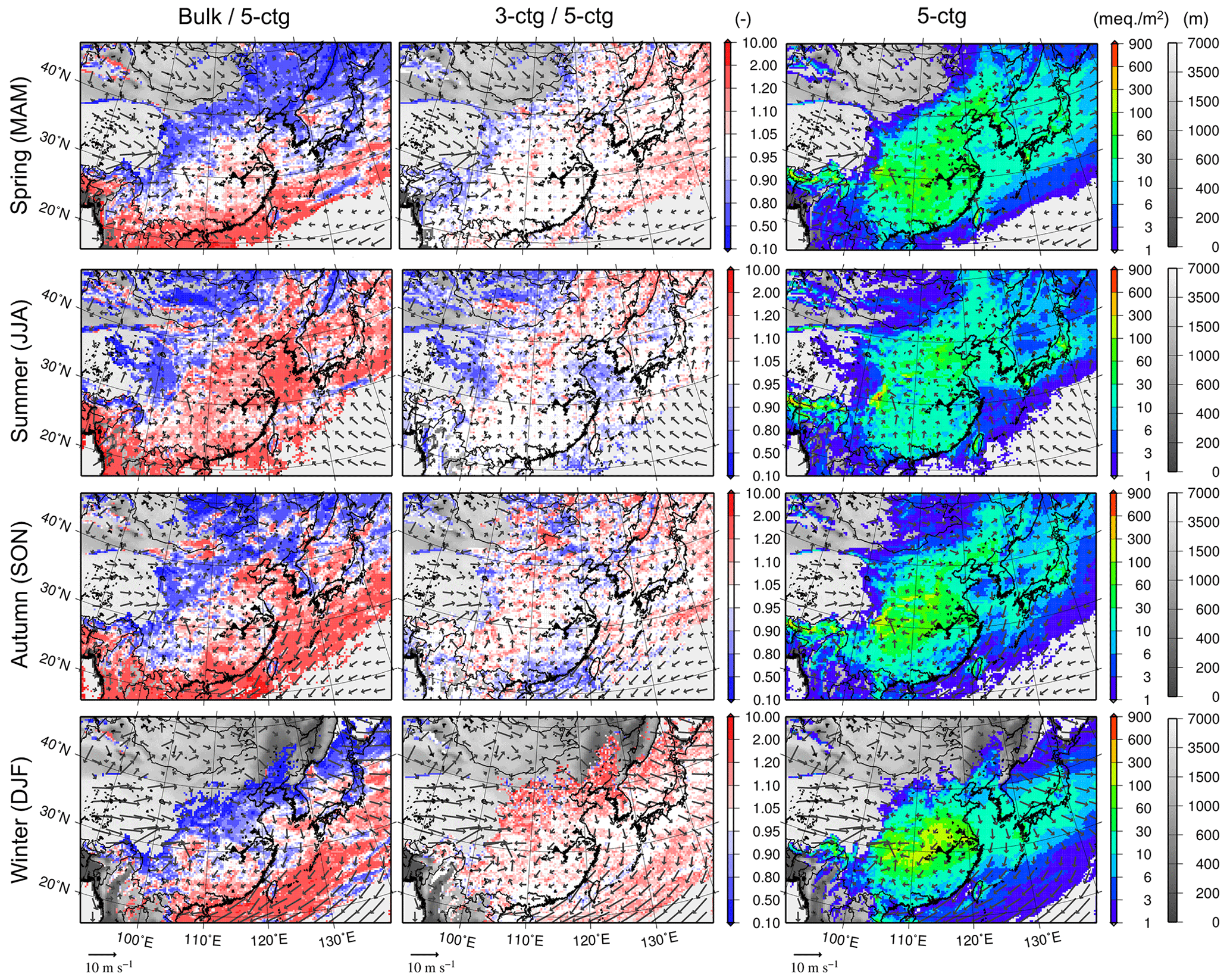
Figure 7Same as Fig. 6 but for wet deposition.
The dry depositions (Fig. 6) of the three-category and five-category methods were very similar (the difference was lower than 5 % in most of the domain) because the size distribution and gas–aerosol partitioning of the components were similar. The separation of soot/soot-free and dust/sea salt particles in the five-category method did not substantially alter the size or gas–aerosol partitioning. The difference between the bulk and five-category methods was significant and varied by up to a factor of 2. This difference is mainly due to difference in the gas–aerosol partitioning of T-, because the differences in nss- and simulated using different methods were less significant. The dry deposition of T- of the bulk method was smaller over land because no coarse-mode was formed over land, where its dry deposition velocity is much larger than that of submicron . Consequently, compared to the other two methods, the total (i.e., nss-, T-, plus T-) dry deposition flux of the bulk method over land was smaller. On the other hand, the total dry deposition of the bulk method is larger over the ocean, where mixed with sea salt was the major component of T-. Because the bulk method assumes instantaneous equilibrium, HNO3 reacts immediately with sea salt particles in the bulk method, whereas HNO3 gradually reacts with sea salt in the five-category method. Consequently, fractions of sea salt mass (as well as T- concentrations) predicted by the bulk method are larger than those of the five-category method, which caused larger dry deposition amounts of T- (as well as the total dry deposition) predicted by the bulk method over the ocean areas.
The horizontal distribution of the wet deposition flux is patchier than that of the dry deposition flux because the horizontal distribution of precipitation is patchy, but similar patterns were found for both fluxes (Fig. 7). The difference in the fluxes between the three-category and five-category methods was small (lower than 10 %–20 % in most of the domain) but larger than the difference in the dry deposition fluxes. The wet deposition of the three-category method was generally larger than that of the five-category method due to the overestimation of wet deposition of , , and mixed with BC, as discussed later in Sect. 6.4.
Fog deposition could be significantly underestimated with a crude grid resolution model, such as in the current study ( km), although it has been significant in local-scale simulations ( km) (e.g., Katata et al., 2011; Kajino et al., 2019b). As the grid resolution becomes cruder, the elevation and slope of the model terrain are more flattened so that the upslope fog formation is underestimated and the low-level clouds cannot reach the model ground surface. It is well known that fog deposition over mountain forests is proportional to elevation (e.g., Katata et al., 2011). The figures are not presented in the main text; however, implementation of a fog deposition scheme was a feature of the current model; the simulated inorganic deposition due to fog is presented and discussed in Supplement 5 and Fig. S5-1 in the Supplement.
6.4 Aerosol optical thickness
Figures 8 and 9 compare the three methods in terms of their predictions of AOT and AAOT at a wavelength of 500 nm integrated from the ground surface up to approximately 1 km a.g.l., respectively.
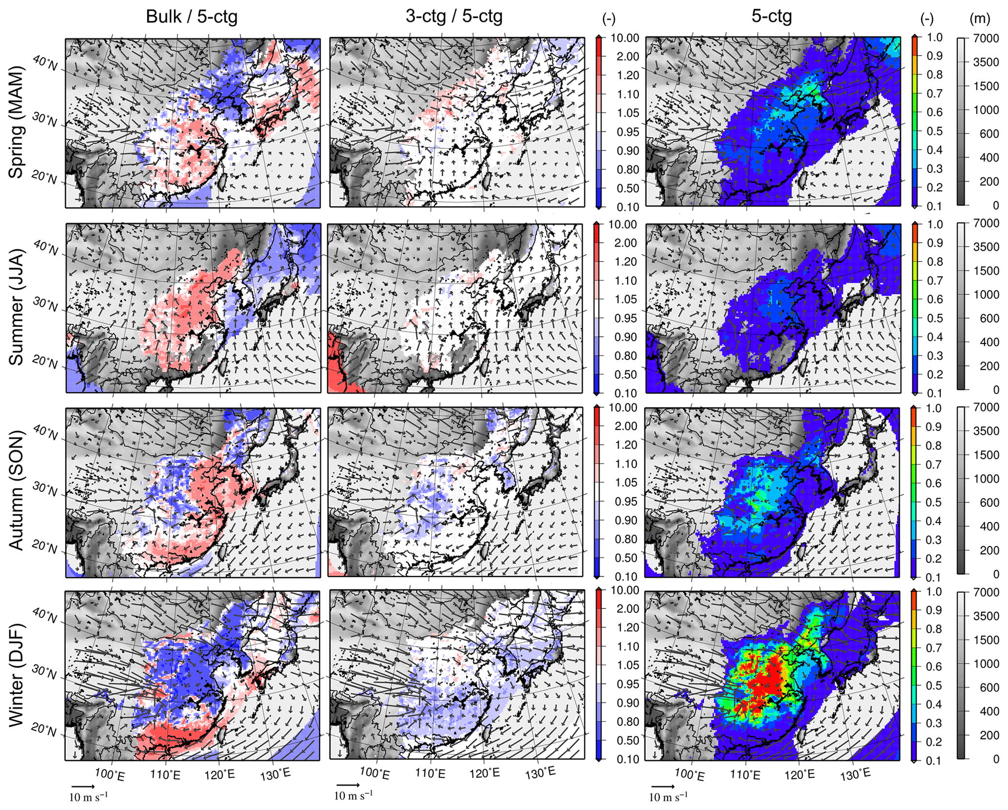
Figure 8Same as Figs. 3–7 but for AOT (at 500 nm) below approximately 1 km a.g.l. The wind vectors are also averaged within 1 km a.g.l.
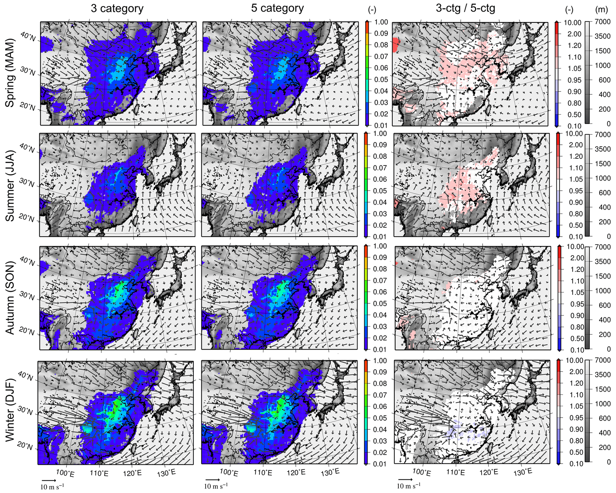
Figure 9Seasonal mean AAOT (at 500 nm) in (top to bottom) spring, summer, autumn, and winter of 2006 for (left to right) the three-category method and the five-category method and the corresponding ratio of the three-category to five-category methods.
AOT and AAOT are both referred to as climate-relevant variables and so the simulations of the three-category and five-category methods are intercompared (the bulk method was not designed for the aerosol feedback studies). However, because data assimilation of AOT observed by satellites is often associated with the operational forecast of aerosol mass concentrations, the bulk method is compared against the other two methods for AOT as presented in Fig. 8. In Figs. 9–11, only the results of the three-category and five-category methods are presented and compared.

Figure 10Same as Fig. 9 but for the total (dry+wet) deposition of BC.
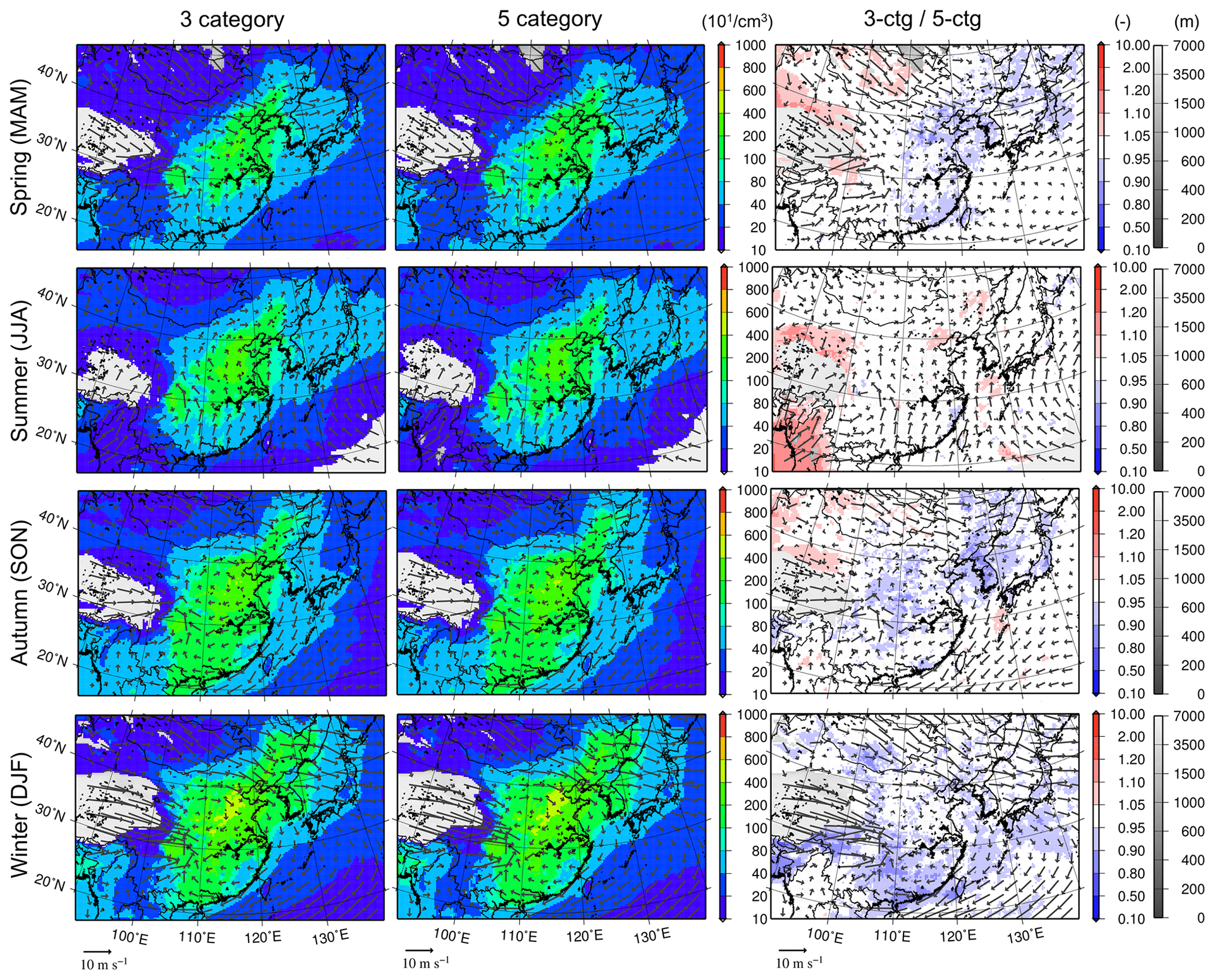
Figure 11Same as Figs. 9 and 10 but for the averaged CCN number concentration below approximately 1 km a.g.l. at a supersaturation of 0.1 %.
Aerosol size distribution is an important parameter for aerosol–cloud–radiation interaction modeling, but the bulk method does not simulate aerosol microphysical processes. Therefore, the bulk method results are not discussed in detail, but the differences between the bulk method results and those from the other two methods considered are large (up to a factor of 2; left panels of Fig. 8). It is only noted here that using different assumptions of size and mixing state (i.e., different settings among the three methods) could cause significant differences in the AOT simulation. This difference should be taken into account when the operational forecast of mass concentration using the bulk method is associated with the data assimilations of optical properties such as AOT. In the large emission source regions and their downwind regions, the differences in AOT between the three-category and five-category methods were small, i.e., smaller than 10 % in most of the domain and seasons. The large difference over the Indian Ocean near the western and southern boundaries of the domain in the summer was due to differences in the internal/external mixture assumptions of soot/soot-free and dust/sea salt at the lateral boundaries. In Fig. 9, the three-category AAOT was slightly larger over the large emission source and their downwind regions (up to 10 %). This was due to the overestimation of the so-called lensing effect (i.e., absorption enhancement by a light-absorbing agent coated by a non-light-absorbing agent; e.g., Bond et al., 2006) by the three-category method, as the soot particles are coated by all of the soot-free components. This is also true for the bulk method. Due to the larger submicron , the overestimation of the lensing effect should be most significant in the bulk method. This trend is also observed in Table 4: sim : obs values of SSA of the five-category, three-category, and bulk methods were 0.95, 0.91, and 0.90, respectively. On the other hand, the internal mixture assumption of the three-category method caused the overestimation of the wet scavenging rates of soot and dust because the soot/soot-free and dust/sea salt particle mixture assumption could make the soot and dust particles larger and more hygroscopic. Consequently, the AAOT of the three-category method was sometimes smaller than that of the five-category method over the downwind regions, but this difference was small (up to 10 %). Figure 10 shows the total (dry+wet) deposition of BC and the differences between the three- and five-category methods. Because the dry deposition velocity of BC is very small, most BC deposition occurred due to wet deposition processes (also indicated by its patchy distribution). This difference was smaller in the spring and summer (reaching overestimation values of up to 10 %) and largest in the winter (20 %–100 %) due to the internal mixture assumption of soot and soot-free particles. Overestimation of the three-category AAOT was more pronounced in the spring and summer than it was in the winter (Fig. 9) because condensation of secondary pollutants to BC was larger in the warmer seasons and because overestimation of the three-category wet deposition of BC was more significant in the winter (Fig. 10). The differences in the total deposition of mineral dust between the three- and five-category methods were very small.
6.5 Aerosol–cloud interactions
The horizontal distributions of the averaged CCN at a supersaturation value of 0.1 % below approximately 1 km a.g.l. are compared in Fig. 11. Whereas the differences in the total CCN between the two methods were very small (up to 10 %), significant differences were observed for some components and occasions of CCN. Figures 12–15 illustrate the scatter diagrams of the simulated daily mean (below-1 km a.g.l.-averaged) CCN (of the three- and five-category methods and at supersaturations of 0.1 % and 1 %) and mass concentrations of all of the model grids, excluding 10 grids from the four lateral boundaries. The numbers of points in the scatter diagrams were randomly reduced to of their value to avoid too many overlaps of symbols. The two supersaturation levels of 0.1 % and 1 % were used for this evaluation as the typical ranges of stratiform and convective clouds (Seinfeld and Pandis, 2006).
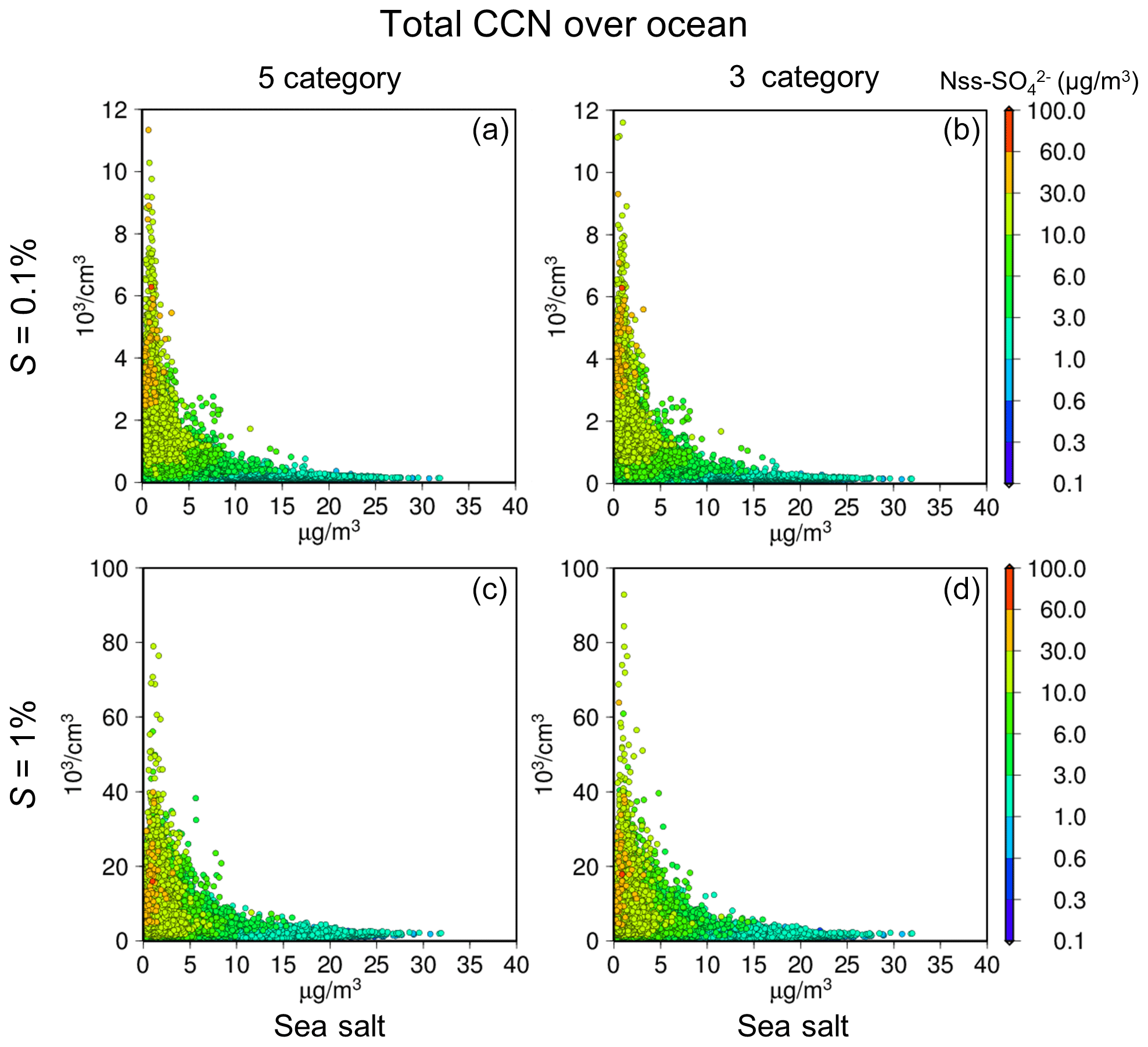
Figure 12Scatter diagrams between the daily mean, averaged below 1 km a.g.l., total CCN number concentrations (y axis) and dry mass concentrations of sea salt (x axis) with nss- concentrations (colors) over the ocean grids for 2006. The number of data points was randomly reduced to approximately to avoid too much overlapping of the points at supersaturation conditions of (a, b) 0.1 % and (c, d) 1 % for (a, c) the five-category and (b, d) three-category methods.
Figure 12 shows the relationship between the total CCN and the sea salt mass over the ocean. In meteorological models, CCN spectra (i.e., the relationship between supersaturation and CCN) are often prescribed, and the CCN over the ocean is often assumed to be 1 order of magnitude lower than that over land (e.g., Rasmussen et al., 2002). However, as the ocean regions in the model domain were located downwind of the large emission source regions, the CCN could be as large as that over the land (e.g., Koike et al., 2012). The simulated total CCN over the ocean areas was up to 2 and 3 orders of magnitude larger than the simulated sea salt particles for both 0.1 % and 1 % supersaturations, respectively (the simulated total CCN reached up to approximately 104 and 105 cm−3 at 0.1 % and 1 %, respectively, while number concentrations of sea salt particles were approximately 100 cm−3 for the mass of 100 µg m−3). The CCN at 1 % was 1 order of magnitude larger than that at 0.1 %. The CCN over the ocean was not correlated with the sea salt mass concentration. The CCN was proportional to the nss- concentrations, an indicator of anthropogenic secondary particles. These results indicate the importance of considering spatiotemporal variations of CCN spectra in the meteorological models, rather than using the prescribed ones that depend only on the LUC (e.g., ocean or land). The CCN difference between the three-category and five-category methods was small, such that the difference in the aerosol–cloud interaction due to CCN changes predicted by the two methods over the ocean could also be small.
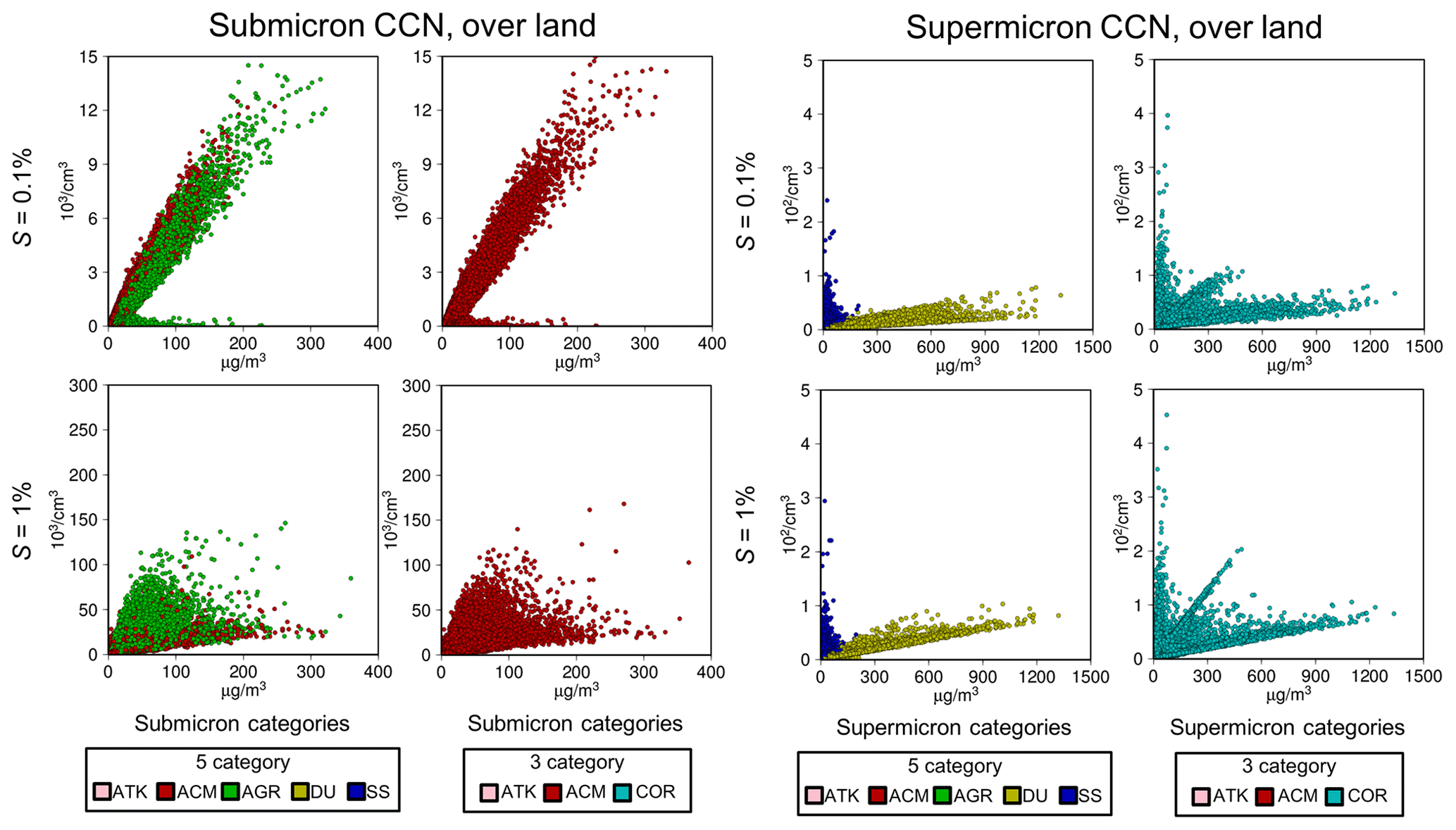
Figure 13Scatter diagrams between the daily mean, averaged below 1 km a.g.l., CCN number concentration (y axis) over the land grids at supersaturation of (top) 0.1 % and (bottom) 1 % from (left four panels) submicron categories (i.e., ATK, ACM, and AGR for the five-category method and ATK and ACM for the three-category method) and (right four panels) supermicron categories (i.e., DU and SS for the five-category method and COR for the three-category method). The x axes are the total dry mass concentrations of the submicron (left four panels) and supermicron (right four panels) categories. The colors of the dots correspond to those of the categories in the legends with the most dominant mass concentrations of the grids.
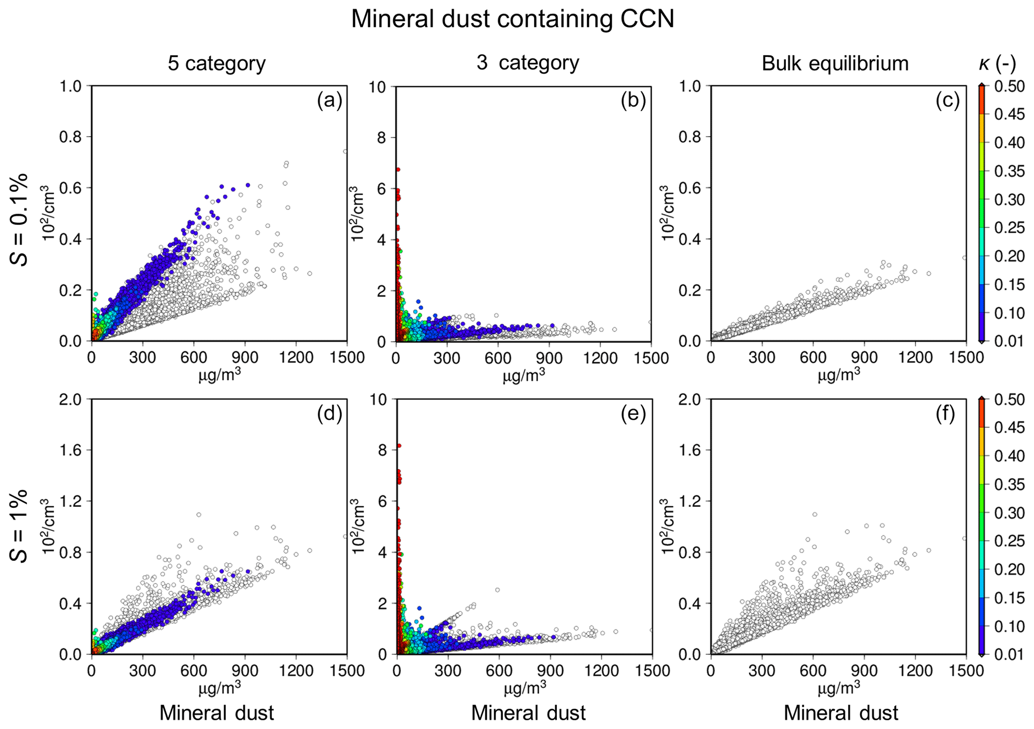
Figure 14Scatter diagrams between the daily mean, averaged below 1 km a.g.l., mineral dust-containing CCN (y axis) at supersaturation of (a–c) 0.1 % and (d–f) 1 % and mineral dust dry mass concentration (x axis) with hygroscopicity κ (colors) for (left to right) the five-category, three-category, and bulk methods. The circles are white if κ is smaller than 0.01.
Figure 13 shows the differences in CCN over land. The submicron CCN at 1 % was 1 order of magnitude larger than that at 0.1 %. The difference in supermicron CCN between 0.1 % and 1 % was not very significant because the larger particles are CCN active at lower supersaturation. There was no difference for hygroscopic sea salt particles, whereas there was a slight difference for less hygroscopic dust particles. Due to the internal mixture assumption of soot and soot-free particles, the CCN at 0.1 % of the three-category method was slightly larger than that of the five-category method. If the model assumes a constant size distribution of submicron particles, all of the points are aligned on a single line. Thus, the width of the aggregations of points indicates the uncertainty or variability of the simulated size distribution of aerosols. The CCN at 0.1 % can vary by approximately 2-fold (e.g., it ranges from 3–6×103 cm−3 at 100 µg m−3 of aerosol mass). The variation (or width) was much larger at 1 %, reaching approximately 1 order of magnitude (5–80×103 cm−3 at 50 µg m−3) because smaller particles can be activated and contribute less to the bulk mass concentration. The accurate prediction of the aerosol population is much more important for the submicron CCN at higher supersaturation values. For supermicron CCN, there are apparent differences in the gradients of lines originated to mineral dust and sea salt in both methods. However, there is one intermediate line in addition to the dust and sea salt lines in the three-category method, which is the result of the unrealistic internal mixture of dust and sea salt. Overall, it is safe to presume that the difference in the aerosol–cloud interaction due to CCN changes predicted by these two methods over land could be small due to the absence of sea salt particles.
Figure 14 illustrates the relationship between mineral-dust-containing CCN and the mineral dust mass concentrations. Because dust is assumed to be inert and κ is assumed to be zero in the bulk method, the CCN at 0.1 % is proportional to only the mineral dust mass concentration, while the variation in the size distribution is more important for the CCN at 1 %. Because the hygroscopic growth of mineral dust is considered in the five-category method, the dust-containing CCN is up to several times larger than that of the bulk method (from 0.1 to 0.4×102 cm−3 at 600 µg m−3). As previously mentioned, the unrealistic internal mixture of dust and sea salt in the three-category method caused unrealistic gradients, i.e., one that is colored in red (sea salt with tiny dust mass) and a line in between (approximately at x=600 µg m−3 and cm−3) that can be clearly seen at 1 % (sea salt–dust mixture). The simulated difference in dust-containing CCN would have almost no impact on CCN–cloud–precipitation interaction processes because its number concentration was much smaller than that of submicron particles. As mineral dust is an efficient INP (e.g., Lohmann and Diehl, 2006), it should be noted here that this difference can have significant impacts on INP–cloud–precipitation interaction processes, especially with immersion freezing (i.e., the freezing of supercooled water droplets containing INPs).
Despite the external mixture treatment of soot and soot-free particles in the five-category method, the difference in the total submicron CCN between the five- and three-category methods was found to be minor (Fig. 13). However, the simulated BC-containing CCN values of the two methods were different, as shown in Fig. 15. The BC-containing CCN of the three-category method at 0.1 % was generally 1.5 times larger than that of the five-category method (e.g., up to 9 and 6×103 cm−3 at 4 µg m−3, respectively) because the absence of BC-free particles causes excess amounts of coatings on BC-containing particles (Oshima et al., 2009b). This difference caused higher BC deposition to be simulated by the three-category method, as presented in Fig. 10. However, the difference in the BC-containing CCN of the two methods at 1 % was not as large as that at 0.1 % because the CCN number concentration at higher supersaturation was not affected by hygroscopicity.
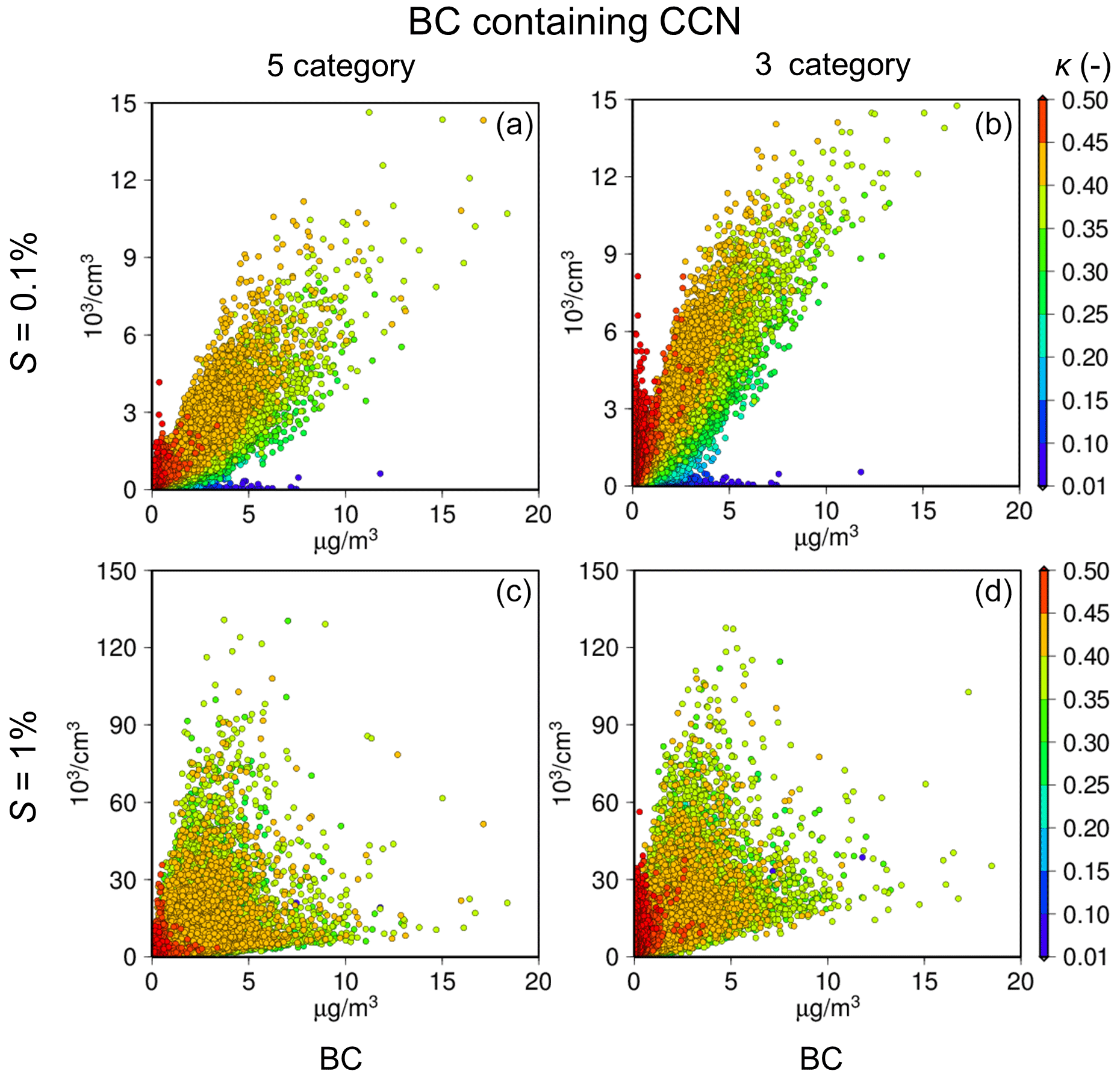
Figure 15Scatter diagrams between the daily mean, averaged below 1 km a.g.l., BC-containing CCN (y axis) at supersaturation of (a, b) 0.1 % and (c, d) 1 % and BC dry mass concentration (x axis) with hygroscopicity κ (colors) for (a, c) the five-category and (b, d) three-category methods.
This study provides a comparison of aerosol representation methods implemented in a regional-scale meteorology–chemistry model (NHM-Chem). Three methods are currently available: the five-category non-equilibrium (Aitken, soot-free accumulation, soot-containing accumulation, sea salt, and dust), three-category non-equilibrium (Aitken, accumulation, and coarse), and bulk equilibrium (submicron, sea salt, and dust) methods. The three methods were intercompared for the predictions of air quality and climate-relevant variables. In this study, surface concentrations and depositions, which negatively impact the human health and environment, are referred to as air quality variables, whereas variables which can alter the Earth's energy budget and water cycles through the aerosol–cloud–radiation interaction processes such as optical properties and cloud and ice nucleation properties are referred to as climate-relevant variables.
The three-category method is widely used in three-dimensional air quality models. The five-category method, the standard method of NHM-Chem, was an extensional development of the three-category method to improve the predictions of aerosol–cloud–radiation interaction processes, by implementing separate treatments of light absorbers and ice nuclei particles, namely, soot and dust, from the accumulation- and coarse-mode categories (implementation of aerosol feedback processes to NHM-Chem is still ongoing). The bulk equilibrium method was developed for operational air quality forecasting with simple aerosol dynamics representations to yield the computational efficiency. The total CPU time of the five-category and three-category methods was 91 % and 44 % greater than the bulk equilibrium method, respectively. The main objective of the study is to quantify the deviations of the widely used three-category method and the efficient bulk equilibrium method from the most realistic aerosol representation of NHM-Chem, the five-category method, and to discuss the magnitude of deviations.
The bulk equilibrium method was evaluated for the eligibility of operational forecast, namely, the surface mass concentrations of air pollutants such as O3, mineral dust, and PM2.5. The differences in the simulated seasonal mean concentrations between the bulk method and the five-category method were smaller than 5 % and 5 %–10 % for O3 and mineral dust, respectively. The difference in PM2.5 was large, i.e., up to 20 %–100 %, due to the neglection of nitrate mixed with dust particles of the bulk equilibrium method. Still, however, the statistical scores of the bulk method regarding PM2.5 were not very different from the other methods. In order to fill the gap between observations and simulations, operational forecast is associated with data assimilation and post-processing of statistical bias correction. The bulk method is not used in recent air quality models any more. Still, however, as the performance among models was similar, the faster bulk equilibrium method can be recommended for the use of operational forecast.
The three-category method was shown to be eligible for air quality simulations, namely, surface concentrations and depositions of bulk chemical species. The differences in the simulated seasonal mean bulk mass concentrations (PM2.5 (pile-up)) and dry and wet depositions of major inorganic components () between the three-category method and the reference method were smaller than 5 %, 5 %, and 10 %, respectively. However, the internal mixture assumption of soot/soot-free and dust/sea salt particles in the three-category method resulted in significant differences in the size distribution and hygroscopicity of the particles. The differences in PM2.5, defined by the simulated size distribution, between the three- and five-category methods were 20 %–100 %.
Although the three-category method was not designed to simulate aerosol–cloud–radiation interaction processes, its performance in terms of total properties, such as AOT and CCN, was acceptable compared to that of the reference method (i.e., both differences were smaller than 10 %). However, some specific parameters exhibited significant differences or systematic errors. For example, the unrealistic dust/sea salt complete mixture of the three-category method induced significant errors in the prediction of mineral dust-containing CCN. The overestimation of soot hygroscopicity by the three-category method induced errors in BC-containing CCN at a supersaturation of 0.1 % (overestimation by ∼50 %), BC deposition (overestimation by 20 %–100 %), and AAOT (difference of <10 %). In contrast, the difference in AAOT was less pronounced because the overestimation of the absorption enhancement was compensated by the overestimation of hygroscopic growth and the consequent loss due to in-cloud scavenging. The five-category method requires more computational resources than the three-category method (44 % in CPU time and 12.5 % in number of tracers, i.e., memory and storage). It should be case dependent which method is recommended but the five-category method tends to be more accurate when the sea salt and dust coexist in the same air mass (such as Gobi dust transport over the northwest Pacific Ocean or the Saharan dust transport over the Mediterranean Sea and the Atlantic Ocean) or when concerning the light absorption and INP activity of BC and dust in the aerosol–cloud–radiation interaction system.
The modal approach was used in the current aerosol microphysics module, but the same conclusion can also be inferred for the sectional (or bin) approaches in terms of the advantage of the five-category approach, namely, the soot and dust sections should be separated from the light-scattering hygroscopic particle section for detailed investigations of aerosol–cloud–radiation interactions. There is a 12-category method that was implemented in a regional model (Glassmeier et al., 2017). This is currently the ultimate representation of the category method in 3-D CTMs. It is necessary to compare our three- and five-category methods to the 12-category approach as a benchmark simulation. The optimization of computational efficiency against complexity (and accuracy) of the aerosol mixing state representations should be achieved via particle analysis studies performed by electron microscopy and particle-resolved models.
There are still large discrepancies between the simulation and observation results, but the reasons are still unclear. In order to identify the reasons and improve NHM-Chem, further evaluations should be made with respect to spatial distributions (using satellites), vertical profiles (using sonde, aircraft, satellite, and lidar), and aerosol size distributions (such as using scanning mobility particle sizer (SMPS), aerodynamic particle sizer (APS), polarized optical particle counter (POPC) methods). There have been tremendous advancements in new particle formation, organic chemistry, and ice nucleation studies. This new knowledge should be immediately reflected in the modeling framework.
To evaluate the significance of separate soot and dust treatments in the five-category method in terms of aerosol–cloud–radiation interaction processes, online simulation with a chemistry-to-meteorology feedback process is required. The sensitivity of aerosol–cloud–radiation interactions to the three aerosol modules will be assessed in the future by the online coupled NHM-Chem with the feedback processes.
The NHM-Chem source code is available subject to a license agreement with the Japan Meteorological Agency. Further information is available at https://www.mri-jma.go.jp/Dep/glb/nhmchem_model/application_en.html (last access: 1 October 2020). The simulation results are free to use. The simulated and observed data used in the paper are available at https://mri-2.mri-jma.go.jp/owncloud/s/ASBzHdtqy9ZpbB4 (Kajino, 2020). The raw observation data of EANET, SKYNET, and AD-Net can be obtained from the websites as described in Sect. 5.
The supplement related to this article is available online at: https://doi.org/10.5194/gmd-14-2235-2021-supplement.
MK designed the current research. MK mainly developed the offline coupled model with MD, who developed its online coupled version. MK and MD collaborated with TTS, NO, KY, TYT, JC, AH, MI, AK, YI, SS, KA, YZ, YI, and TM during model development. MK performed the simulations, which were evaluated by the observation data provided by TY, MM (Miyashita), PK, AS, and HI. YI, HU, TM, and MM (Mikami) co-supervised this study.
The authors declare that they have no conflict of interest.
The authors thank Toshinori Aoyagi of the JMA, Mitsuo Ohizumi of Meteorological College, and Hiroaki Naoe, Masashi Niwano, and Masaya Nosaka of the MRI for their useful comments on model developments. The authors are deeply grateful for the support of Shohei Suzuki and Kazuki Ito of the University of Tsukuba for the visualization of simulation and observation data and Kyoko Kaneba for the comments on the manuscript. The authors also thank the Kagoshima Meteorological Office and Aso Volcano Disaster Prevention Council for providing the volcanic SO2 emission measurement data of Mt. Sakurajima and Mt. Aso, respectively.
This work was mainly supported by the Fundamental Technology Research of MRI (M5 and P5), the Integrated Research Program for Advancing Climate Models (TOUGOU) grant no. JPMXD0717935561 and Arctic Challenge for Sustainability II (ArCS II), grant no. JPMXD1420318865 from the Ministry of Education, Culture, Sports, Science, and Technology Japan (MEXT), and Research Institute for Humanity and Nature (RIHN: a constituent member of NIHU) project no. 14200133 (Aakash). This work was also supported by the Japanese Society for the Promotion of Sciences (JSPS) KAKENHI grant nos. JP19H01155, JP16KK0018, JP19F19402, JP19H02649, JP18H03363, JP18H05292, and JP2000636) and the Environment Research and Technology Development Fund (grant nos. JPMEERF20165005, JPMEERF20172003, JPMEERF14S11203, JPMEERF20202003, JPMEERF20205001, and JPMEERF20215003) of the Environmental Restoration and Conservation Agency of Japan and in part by a grant for the Global Environmental Research Coordination System from the Ministry of Environment, Japan (MOEJ) (grant no. MLIT1753).
This paper was edited by Holger Tost and reviewed by two anonymous referees.
Aquila, V., Hendricks, J., Lauer, A., Riemer, N., Vogel, H., Baumgardner, D., Minikin, A., Petzold, A., Schwarz, J. P., Spackman, J. R., Weinzierl, B., Righi, M., and Dall'Amico, M.: MADE-in: a new aerosol microphysics submodel for global simulation of insoluble particles and their mixing state, Geosci. Model Dev., 4, 325–355, https://doi.org/10.5194/gmd-4-325-2011, 2011.
Aoki, T., Tanaka, T. Y., Uchiyama, A., Chiba, M., Mikami, M., Yabuki, S., and Key, J. R.: Sensitivity experiments of direct radiative forcing caused by mineral dust simulated with a chemical transport model, J. Meteorol. Soc. Jpn., 83A, 315–331, 2005.
Aranami, K., Hara, T., Ikuta, Y., Kawano, K., Matsubayashi, K., Kusabiraki, H., Ito, T., Egawa, T., Yaashita, K., Ota, Y., Ishikawa, Y. Fujita, T., and Ishida, J.: A new operational regional model for convection-permitting numerical weather prediction at JMA, CAS/JSC WGNE, Research Activities in Atmospheric and Oceanic Modelling, 5, 5–6, 2015.
Bond, T. C., Habib, G., and Bergstrom, R. W.: Limitations in the enhancement of visible light absorption due to mixing state, J. Geophys. Res., 111, D20211, https://doi.org/10.1029/2006JD007315, 2006.
Bond, T. C., Doherty, S. J., Fahey, D. W., Forster, P. M., Berntsen, T., DeAngelo, B. J., Flanner, M. G., Ghan, S., Kärcher, B., Koch, D., Kinne, S., Kondo, Y., Quinn, P. K., Sarofim, M. C., Schultz, M. G., Schlz, M., Venkataraman, C., Zhang, H., Zhang, S., Bellouin, N., Guttikunda, S. K., Hopke, P. K., Jacobson, M. Z., Kaiser, J. W., Klimont, Z., Lohmann, U., Schwarz, J. P., Shindell, D., Storelvmo, T., Warren, S. G., and Zender, C. S.: Bounding the role of black carbon in the climate system: A scientific assessment, J. Geophys. Res., 118, 1–173, 2013.
Boucher, O., Randall, D., Artaxo, P., Bretherton, C., Feingold, G., Forster, P., Kerminen, V.-M., Kondo, Y., Liao, H., Lohmann, U., Rasch, P., Satheesh, S. K., Sherwood, S., Stevens, B., and Zhang, X. Y.: Clouds and aerosols, in: Climate Change 2013: the Physical Science Basis, Working Group I Contribution to the Fifth Assessment Report of the Intergovernmental Panel on Climate Change, edited by: Stocker, T. F., Cambridge Univ. Press, New York, 571–657, 2013.
Burns, D. A., Lynch, J. A., Cosby, B. J., Fenn, M. E., Baron, J. S., US EPA Clean Air Markets Div.: National Acid Precipitation Assessment Program Report to Congress 2011: An integrated assessment, National Science and Technology Council, Washington, DC, 114 pp., 2011.
Byun, D. and Schere K.: Review of the governing equations, computational algorithms, and other components of the Models-3 Community Multiscale Air Quality (CMAQ) modeling system, Appl. Mech. Rev., 59, 51–77, 2006.
Carlton, A. G., Turpin, B. J., Altieri, K. E., Seitzinger, S., Reff, A., Lim, H.-J., and Ervens, B.: Atmospheric oxalic acid and SOA production from glyoxal: Results of aqueous photooxidation experiment, Atmos. Environ., 41, 7588–7602, 2007.
Carter, W.: Documentation of the SAPRC-99 chemical mechanism for VOC reactivity assessment, Final report to California Air Resources Board, Rep. 92–329, Univ. of Calif., Riverside, 8 May, 569 pp., 2000.
Chapman, E. G., Gustafson Jr., W. I., Easter, R. C., Barnard, J. C., Ghan, S. J., Pekour, M. S., and Fast, J. D.: Coupling aerosol-cloud-radiative processes in the WRF-Chem model: Investigating the radiative impact of elevated point sources, Atmos. Chem. Phys., 9, 945–964, https://doi.org/10.5194/acp-9-945-2009, 2009.
Ching, J., Riemer, N., and West, M.: Impacts of black carbon mixing state on black carbon nucleation scavenging: Insights from a particle-resolved model, J. Geophys. Res., 117, D23209, 2012.
Ching, J., Zaveri, R. A., Easter, R. C., Riemer, N., and Fast, J. D.: A three-dimensional sectional representation of aerosol mixing state for simulating optical properties and cloud condensation nuclei, J. Geophys. Res., 121, 5912–5929, 2016a.
Ching, J., Riemer, N., and West, M.: Impacts of black carbon particles mixing state on cloud microphysical properties: Sensitivity to environmental conditions, J. Geophys. Res., 121, 5990–6013, 2016b.
Ching, J., Fast, J., West, M., and Riemer, N.: Metrics to quantify the importance of mixing state for CCN activity, Atmos. Chem. Phys., 17, 7445–7458, https://doi.org/10.5194/acp-17-7445-2017, 2017.
Ching, J., West, M., and Riemer, N.: Quantifying impacts of aerosol mixing state on nucleation-scavenging of black carbon aerosol particles, Atmosphere, 9, 17, 17 pp., 2018.
Clarke, A. D., Owens, S. R., and Zhou, J.: An ultrafine sea-salt flux from breaking waves: Implications for cloud condensation nuclei in the remote marine atmosphere, J. Geophys. Res., 111, D06202, https://doi.org/10.1029/2005JD006565, 2006.
Cohen, A. J., Anderson, H. R., Ostro, B., Pandey, K. D., Krzyzanowski, M., Künzli, N., Gutschmidt, K., Pope III, C. A., Romieu, I., Samet, J. M., and Smith, K. R.: Urban air pollution, in Comparative Quantification of Health Risks: Global and Regional Burden of Disease Attributable to Selected Major Risk Factors, 1st Edn., edited by: Ezzati, M., Lopez, A. D., Rodgers, A., and Murray, C. J. L., World Health Organization, Geneva, Vol. 2, 1353–1453, 2004.
Curtis, J. H., Riemer, N., and West, M.: A single-column particle-resolved model for simulating the vertical distribution of aerosol mixing state: WRF-PartMC-MOSAIC-SCM v1.0, Geosci. Model Dev., 10, 4057–4079, https://doi.org/10.5194/gmd-10-4057-2017, 2017.
Deushi, M. and Shibata, K.: Development of an MRI Chemistry-Climate Model ver.2 for the study of tropospheric and stratospheric chemistry, Papers in Meteor. Geophys., 62, 1–46, 2011.
Edney, E. O., Kleindienst, T. E., Lewandowski, M., and Offenberg, J. H.: Updated SOA chemical mechanism for the Community Multiscale Air Quality model, EPA 600/X-07/025, US Environ. Prot. Agency, Durham, NC, 2007.
Facchini, M. C., Rinaldi, M., Decesari, S., Carbone, C., Finessi, E., Mircea, M., Fuzzi, S., Ceburnis, D., Flanagan, R., Nilsson, E. D., de Leeuw, G., Martino, M., Woeltjen, J., and O'Dowd, C. D.: Primary submicron marine aerosol dominated by insoluble organic colloids and aggregates, Geophys. Res. Lett., 35, L17814, https://doi.org/10.1029/2008GL034210, 2008.
Fountoukis, C. and Nenes, A.: ISORROPIA II: a computationally efficient thermodynamic equilibrium model for K+-Ca2+-Mg2+-NH4+-Na+---Cl−-H2O aerosols, Atmos. Chem. Phys., 7, 4639–4659, https://doi.org/10.5194/acp-7-4639-2007, 2007.
Giglio, L., Randerson, J. T., van der Werf, G. R., Kasibhatla, P. S., Collatz, G. J., Morton, D. C., and DeFries, R. S.: Assessing variability and long-term trends in burned area by merging multiple satellite fire products, Biogeosciences, 7, 1171–1186, https://doi.org/10.5194/bg-7-1171-2010, 2010.
Glassmeier, F., Possner, A., Vogel, B., Vogel, H., and Lohmann, U.: A comparison of two chemistry and aerosol schemes on the regional scale and the resulting impact on radiative properties and liquid- and ice-phase aerosol–cloud interactions, Atmos. Chem. Phys., 17, 8651–8680, https://doi.org/10.5194/acp-17-8651-2017, 2017.
Grell, G. A., Peckham, S. E., Schmitz, R., McKeen, S. A., Frost, G., Skamarock, W. C., and Eder, B.: Fully coupled “online” chemistry within the WRF model, Atmos. Environ., 39, 6957–6975, 2005.
Guenther, A., Karl, T., Harley, P., Wiedinmyer, C., Palmer, P. I., and Geron, C.: Estimates of global terrestrial isoprene emissions using MEGAN (Model of Emissions of Gases and Aerosols from Nature), Atmos. Chem. Phys., 6, 3181–3210, https://doi.org/10.5194/acp-6-3181-2006, 2006.
Han, Z., Ueda, H., Matsuda, K., Zhang, R.., Arao, K., Kanai, Y., and Hasome, H.: Model study on particle size segregation and deposition during Asian dust events in March 2002, J. Geophys. Res., 109, D19205, https://doi.org/10.1029/2004JD004920, 2004.
Hess, M., Koepke, P., and Schult, I.: Optical properties of aerosols and clouds: the software package OPAC, B. Am. Meteorol. Soc., 79, 831–844, 1998.
Itahashi, S., Ge, B., Sato, K., Fu, J. S., Wang, X., Yamaji, K., Nagashima, T., Li, J., Kajino, M., Liao, H., Zhang, M., Wang, Z., Li, M., Kurokawa, J., Carmichael, G. R., and Wang, Z.: MICS-Asia III: overview of model intercomparison and evaluation of acid deposition over Asia, Atmos. Chem. Phys., 20, 2667–2693, https://doi.org/10.5194/acp-20-2667-2020, 2020.
Jacob, D. J.: Heterogeneous chemistry and tropospheric ozone, Atmos. Environ., 34, 2131–2159, 2000.
Jacobson, M. Z.: Analysis of aerosol interactions with numerical techniques for solving coagulation, nucleation, condensation, dissolution, and reversible chemistry among multiple size distributions, J. Geophys. Res., 107, 4366, https://doi.org/10.1029/2001JD002044, 2002.
JMA: The next generation non-hydrostatic model ASUCA, Suuchi Yohoka Hokoku Bessatsu (Additonal Volume to Report of Numerical Prediction Division), 60, 151 pp., 2014 (in Japanese).
Kajino, M.: GMD_3aeroComp_PubData, Meteorological Research Institute, available at: https://mri-2.mri-jma.go.jp/owncloud/s/ASBzHdtqy9ZpbB4, last access: 14 September 2020.
Kajino, M., Ueda, H., Satsumabayashi, H., and An, J.: Impacts of the eruption of Miyakejima Volcano on air quality over far east Asia, J. Geophys. Res., 109, D21204, https://doi.org/10.1029/2004JD004762, 2004.
Kajino, M. and Kondo, Y.: EMTACS: Development and regional-scale simulation of a size, chemical, mixing type, and soot shape resolved atmospheric particle model, J. Geophys. Res., 116, D02303, https://doi.org/10.1029/2010JD015030, 2011.
Kajino, M., Inomata, Y., Sato, K., Ueda, H., Han, Z., An, J., Katata, G., Deushi, M., Maki, T., Oshima, N., Kurokawa, J., Ohara, T., Takami, A., and Hatakeyama, S.: Development of the RAQM2 aerosol chemical transport model and predictions of the Northeast Asian aerosol mass, size, chemistry, and mixing type, Atmos. Chem. Phys., 12, 11833–11856, https://doi.org/10.5194/acp-12-11833-2012, 2012a.
Kajino, M., Deushi, M., Maki, T., Oshima, N., Inomata, Y., Sato, K., Ohizumi, T., and Ueda, H.: Modeling wet deposition and concentration of inorganics over Northeast Asia with MRI-PM/c, Geosci. Model Dev., 5, 1363–1375, https://doi.org/10.5194/gmd-5-1363-2012, 2012b.
Kajino, M., Sato, K., Inomata, Y., and Ueda, H.: Source-receptor relationships of nitrate in Northeast Asia and influence of sea salt on the long-range transport of nitrate, Atmos. Environ., 79, 67–78, 2013.
Kajino, M., Ueda, H., Han, Z., Kudo, R., Inomata, Y., and Kaku, H.: Synergy between air pollution and urban meteorological changes through aerosol-radiation-diffusion feedback – A case study of Beijing in January 2013, Atmos. Environ., 171, 98–110, 2017.
Kajino, M., Deushi, M., Sekiyama, T. T., Oshima, N., Yumimoto, K., Tanaka, T. Y., Ching, J., Hashimoto, A., Yamamoto, T., Ikegami, M., Kamada, A., Miyashita, M., Inomata, Y., Shima, S., Takami, A., Shimizu, A., Hatakeyama, S., Sadanaga, Y., Irie, H., Adachi, K., Zaizen, Y., Igarashi, Y., Ueda, H., Maki, T., and Mikami, M.: NHM-Chem, the Japan Meteorological Agency's regional meteorology – chemistry model: model evaluations toward the consistent predictions of the chemical, physical, and optical properties of aerosols, J. Meteor. Soc. Jpn., 97, 337–374, https://doi.org/10.2151/jmsj.2019-020, 2019a.
Kajino, M., Sekiyama, T. T., Igarashi, Y., Katata, G., Sawada, M., Adachi, K., Zaizen, Y., Tsuruta, H., and Nakajima, T.: Deposition and dispersion of radio-cesium released due to the Fukushima nuclear accident: Sensitivity to meteorological models and physical modules, J. Geophys. Res., 124, 1823–1845, https://doi.org/10.1029/2018JD028998, 2019b.
Kajino, M., Hayashida, S., Sekiyama, T. T., Deushi, M., Ito, K., and Liu, X.: Detectability assessment of a satellite sensor for lower tropospheric ozone responses to its precursors emission changes in East Asian summer, Sci. Rep., 9, 19629, https://doi.org/10.1038/s41598-019-55759-7, 8 pp., 2019c.
Kajino, M., Hagino, H., Fujitani, Y., Morikawa, T., Fukui, T., Onishi, K., Okuda, T., and Igarashi, Y.: Modeling transition metals in East Asia and Japan toward the predictions of aerosol oxidative potential and its emission sources, GeoHealth, 4, e2020GH000259, https://doi.org/10.1029/2020GH000259, 2020.
Kajino, M., Sekiyama, T. T., Igarashi, Y., Katata, G., Sawada, M., Adachi, K., Zaizen, Y., Tsuruta, H., Nakajima, T.: Deposition and dispersion of radio-cesium released due to the Fukushima nuclear accident: 2. Sensitivity to aerosol microphysical propertis of Cs-bearing microparticles (CsMPs), J. Geophys. Res., 126, e2020JD033460, https://doi.org/10.1029/2020JD033460, 2021.
Kameda, T., Azumi, E., Fukushima, A., Tang, N., Matsuki, A., Kamiya, Y., Toriba, A., and Hayakawa, K.: Mineral dust aerosols promote the formation of toxic nitropolycyclic aromatic compounds, Sci. Rep., 6, 24427, https://doi.org/10.1038/srep24427, 2016.
Kaneyasu, N., Ohashi, H., Suzuki, F., Okuda, T., and Ikemori, F.: Sulfate aerosol as a potential transport medium of radiocesium from the Fukushima nuclear accident, Environ. Sci. Technol., 46, 5720–5726, https://doi.org/10.1021/es204667h, 2012.
Katata, G., Kajino, M., Hiraki, T., Aikawa, M., Kobayashi, T., and Nagai, H.: A method for simple and accurate estimation of fog deposition in a mountain forest using a meteorological model, J. Geophys. Res., 116, D20102, https://doi.org/10.1029/2010JD015552, 2011.
Katata, G., Chino, M., Kobayashi, T., Terada, H., Ota, M., Nagai, H., Kajino, M., Draxler, R., Hort, M. C., Malo, A., Torii, T., and Sanada, Y.: Detailed source term estimation of the atmospheric release for the Fukushima Daiichi Nuclear Power Station accident by coupling simulations of an atmospheric dispersion model with an improved deposition scheme and oceanic dispersion model, Atmos. Chem. Phys., 15, 1029–1070, https://doi.org/10.5194/acp-15-1029-2015, 2015.
Kobayashi, S., Ota, Y., Harada, Y., Ebita, A., Moriya, M., Onda, H., Onogi, K., Kamahori, H., Kobayashi, C., Endo, H., Miyaoka, K., and Takahashi, K.: The JRA-55 Reanalysis: General specifications and basic characteristics, J. Meteor. Soc. Jpn., 93, 5–48, 2015.
Koike, M., Takegawa, N., Moteki, N., Kondo, Y., Nakamura, H., Kita, K., Matsui, H., Oshima, N., Kajino, M., and Nakajima, T. Y.: Measurements of regional-scale aerosol impacts on cloud microphysics over the East China Sea: Possible influences of warm sea surface temperature over the Kuroshio ocean current, J. Geophys. Res., 117, D17205, https://doi.org/10.1029/2011JD017324, 012.
Kondo, Y., Oshima, N., Kajino, M., Mikami, R., Moteki, N., Takegawa, N., Verma, R. L., Kajii, Y., Kato, S., and Takami, A.: Emissions of black carbon in East Asia estimated from observations at a remote site in the East China Sea, J. Geophys. Res., 116, D16201, https://doi.org/10.1029/2011JD015637, 2011.
Kurokawa, J., Ohara, T., Morikawa, T., Hanayama, S., Janssens-Maenhout, G., Fukui, T., Kawashima, K., and Akimoto, H.: Emissions of air pollutants and greenhouse gases over Asian regions during 2000–2008: Regional Emission inventory in ASia (REAS) version 2, Atmos. Chem. Phys., 13, 11019–11058, https://doi.org/10.5194/acp-13-11019-2013, 2013.
Li, J., Nagashima, T., Kong, L., Ge, B., Yamaji, K., Fu, J. S., Wang, X., Fan, Q., Itahashi, S., Lee, H.-J., Kim, C.-H., Lin, C.-Y., Zhang, M., Tao, Z., Kajino, M., Liao, H., Li, M., Woo, J.-H., Kurokawa, J., Wang, Z., Wu, Q., Akimoto, H., Carmichael, G. R., and Wang, Z.: Model evaluation and intercomparison of surface-level ozone and relevant species in East Asia in the context of MICS-Asia Phase III – Part 1: Overview, Atmos. Chem. Phys., 19, 12993–13015, https://doi.org/10.5194/acp-19-12993-2019, 2019.
Li, M., Zhang, Q., Kurokawa, J.-I., Woo, J.-H., He, K., Lu, Z., Ohara, T., Song, Y., Streets, D. G., Carmichael, G. R., Cheng, Y., Hong, C., Huo, H., Jiang, X., Kang, S., Liu, F., Su, H., and Zheng, B.: MIX: a mosaic Asian anthropogenic emission inventory under the international collaboration framework of the MICS-Asia and HTAP, Atmos. Chem. Phys., 17, 935–963, https://doi.org/10.5194/acp-17-935-2017, 2017.
Liu, X., Easter, R. C., Ghan, S. J., Zaveri, R., Rasch, P., Shi, X., Lamarque, J.-F., Gettelman, A., Morrison, H., Vitt, F., Conley, A., Park, S., Neale, R., Hannay, C., Ekman, A. M. L., Hess, P., Mahowald, N., Collins, W., Iacono, M. J., Bretherton, C. S., Flanner, M. G., and Mitchell, D.: Toward a minimal representation of aerosols in climate models: description and evaluation in the Community Atmosphere Model CAM5, Geosci. Model Dev., 5, 709–739, https://doi.org/10.5194/gmd-5-709-2012, 2012.
Liu, X., Ma, P.-L., Wang, H., Tilmes, S., Singh, B., Easter, R. C., Ghan, S. J., and Rasch, P. J.: Description and evaluation of a new four-mode version of the Modal Aerosol Module (MAM4) within version 5.3 of the Community Atmosphere Model, Geosci. Model Dev., 9, 505–522, https://doi.org/10.5194/gmd-9-505-2016, 2016.
Lohmann, U. and Diehl, K.: Sensitivity studies of the importance of dust ice nuclei for the indirect aerosol effect on stratiform mixedphase clouds, J. Atmos. Sci., 63, 968–982, 2006.
Matsui, H.: Development of a global aerosol model using a two-dimensional sectional method: 1. Model design, J. Adv. Model. Earth Sy., 9, 1921–1947, 2017.
Miyakawa, T., Takeda, N., Koizumi, K., Tabaru, M., Ozawa, Y., Hirayama, N., and Takegawa, N.: A new lase induced incandescence – mass spectrometric analyzer (LII-MS) for online measurement of aerosol composition classified by black carbon mixing state, Aerosol Sci. Tech., 48, 853–863, 2014.
Nakajima, T., Yoon, S. C., Ramanathan, V., Shi, G. Y., Takemura, T., Higurashi, A., Takamura, T., Aoki, K., Sohn, B. J., Kim, S. W., Tusuruta, H., Sugimoto, N., Shimizu, A., Tanimoto, H., Sawa, Y., Lin, N. H., Lee, C. T., Goto, D., and Schutgens, N.: Overview of the Atmospheric Brown Cloud East Asian Regional Experiment 2005 and a study of the aerosol direct radiative forcing in east Asia, J. Geophys. Res., 112, D24S91, https://doi.org/10.1029/2007JD009009, 2007.
Nakano, M., Kato, T., Hayashi, S., Kanada, S., Yamada, Y., and Kurihara, K.: Development of a 5-km-Mesh Cloud-System-Resolving Regional Climate Model at the Meteorological Research Institute, J. Meteorol. Soc. Jpn., 90A, 339–350, 2012.
Nishizawa, S., Yashiro, H., Sato, Y., Miyamoto, Y., and Tomita, H.: Influence of grid aspect ratio on planetary boundary layer turbulence in large-eddy simulations, Geosci. Model Dev., 8, 3393–3419, https://doi.org/10.5194/gmd-8-3393-2015, 2015.
Oshima, N. and Koike, M.: Development of a parameterization of black carbon aging for use in general circulation models, Geosci. Model Dev., 6, 263–282, https://doi.org/10.5194/gmd-6-263-2013, 2013.
Oshima, N., Koike, M., Zhang, Y., Kondo, Y., Moteki, N., Takegawa, N., and Miyazaki, Y.: Aging of black carbon in outflow from anthropogenic sources using a mixing state resolved model: Model development and evaluation, J. Geophys. Res., 114, D06210, https://doi.org/10.1029/2008JD010680, 2009a.
Oshima, N., Koike, M., Zhang, Y., and Kondo, Y.: Aging of black carbon in outflow from anthropogenic sources using a mixing state resolved model: 2. Aerosol optical properties and cloud condensation nuclei activities, J. Geophys. Res., 114, D18202, https://doi.org/10.1029/2008JD011681, 2009b.
Oshima, N., Kondo, Y., Moteki, N., Takegawa, N., Koike, M., Kita, K., Matsui, H., Kajino, M., Nakamura, H., Jung, J. S., and Kim, Y. J.: Wet removal of black carbon in Asian outflow: Aerosol Radiative Forcing in East Asia (A-FORCE) aircraft campaign, J. Geophys. Res., 117, D03204, https://doi.org/10.1029/2011JD016552, 2012.
Oshima, N., Koike, M., Kondo, Y., Nakamura, H., Moteki, N., Matsui, H., Takegawa, N., and Kita, K.: Vertical transport mechanisms of black carbon over East Asia in spring during the A-FORCE aircraft campaign, J. Geophys. Res.-Atmos., 118, 13175–13198, https://doi.org/10.1002/2013JD020262, 2013.
Oshima, N., Yukimoto, S., Deushi, M., Koshiro, T., Kawai, H., Tanaka, T. Y., and Yoshida, K.: Global and Arctic effective radiative forcing of anthropogenic gases and aerosols in MRI-ESM2.0, Progress in Earth and Planetary Science, 7, 38, https://doi.org/10.1186/s40645-020-00348-w, 2020.
Petters, M. D. and Kreidenweis, S. M.: A single parameter representation of hygroscopic growth and cloud condensation nucleus activity, Atmos. Chem. Phys., 7, 1961–1971, https://doi.org/10.5194/acp-7-1961-2007, 2007.
Pleim, J. E. and Chang, J. S.: A non-local closure model for vertical mixing in the convective boundary layer, Atmos. Environ., 26A, 965–981, 1992.
Prather, K. A., Bertram, T. H., Grassian, V. H., Deane, G. B., Stokes, M. D., Demott, P. J., Aluwihare, L. I., Palenik, B. P., Azam, F., Seinfeld, J. H., Moffet, R. C., Molina, M. J., Cappa, C. D., Geiger, F. M., Roberts, G. C., Russel, L. M., Ault, A. P., Baltrusaitis, J., Collins, D. B., Corrigan, C. E., Cuadra-Rodriguez, L. A., Ebben, C. J., Forestieri, S. D., Guasco, T. L., Hersey, S. P., Kim, M. J., Lambert, W. F., Modini, R. L., Mui, W., Pedler, B. E., Ruppel, M. J., Ryder, O. S., Schoepp, N. G., Sullivan, R. C., and Zhao, D.: Bringing the ocean into the laboratory to probe the chemical complexity of sea spray aerosol, Proc. Natl. Acad. Sci., 110(19), 7550–7555, 2013.
Pringle, K. J., Tost, H., Message, S., Steil, B., Giannadaki, D., Nenes, A., Fountoukis, C., Stier, P., Vignati, E., and Lelieveld, J.: Description and evaluation of GMXe: a new aerosol submodel for global simulations (v1), Geosci. Model Dev., 3, 391–412, https://doi.org/10.5194/gmd-3-391-2010, 2010.
Rasmussen, R. M., Geresdi, I., Thompson, G., Manning, K., and Karplus, E.: Freezing drizzle formation in stably stratified layer clouds: The role of radiation cooling of cloud droplets, cloud condensation nuclei, and ice initiation, J. Atmos. Sci., 59, 837–860, 2002.
Riemer, N., Vogel, H., Vogel, B., and Fiedler, F.: Modeling aerosols on the mesoscale-γ: Treatment of soot aerosol and its radiative effects, J. Geophys. Res., 108, 4601, https://doi.org/10.1029/2003JD003448, 2003.
Riemer, N., West, M., Zaveri, R. A., and Easter, R. C.: Simulating the evolution of soot mixing state with a particle-resolved aerosol model, J. Geophys. Res., 114, D09202, https://doi.org/10.1029/2008JD011073, 2009.
Rosenfeld, D., Lohmann, U., Raga, G. B., O'Dowd, C. D., Kulmala, M., Fuzzi, S., Reissell, A., and Andreae M. O.: Flood or drought: how do aerosols affect precipitation?, Science, 321, 1309–1313, 2008.
Saito, K.: Chapter 5. The JMA nonhydrostatic model and its application to operation and research, Atmospheric Model Applications, edited by: Yucel, I., InTech Open Access Publisher, 85–110, 2012.
Saito, K., Fujita, T., Yamada, Y., Ishida, J., Kumagai, Y., Aranami, K., Ohmori, S., Nagasawa, R., Kumagai, S., Muroi, C., Kato, T., Eito, H., and Yamazaki, Y.: The operational JMA nonhydrostatic mesoscale model, Mon. Weather Rev., 134, 1266–1298, 2006.
Saito, K., Ishida, J., Aranami, K., Hara, T., Segawa, T., Narita, M., and Honda, Y.: Nonhydrostatic atmospheric models operational development at JMA, J. Meteor. Soc. Jpn., 85B, 271–304, 2007.
Sato, Y., Nishizawa, S., Yashiro, H., Miyamoto, Y., Kajikawa, Y., and Tomita, H.: Impacts of cloud microphysics on trade wind cumulus: which cloud microphysics processes contribute to the diversity in a large eddy simulation?, Progress in Earth and Planetary Science, 2, 23, https://doi.org/10.1186/s40645-015-0053-6, 2015.
Sato, Y., Sekiyama, T. T. , Fang, S. , Kajino, M., Quérel, A., Quélo, D., Kondo, H., Terada, H., Kadowaki, M., Takigawa, M., Morino, Y., Uchida, J., Goto, D., and Yamazawa, H.: A Model intercomparison of atmospheric 137Cs concentrations from the Fukushima Daiichi Nuclear Power Plant accident, Phase III: Simulation with an identical source term and meteorological field at 1 km resolution, Atmos. Environ. X, 7, 100086, https://doi.org/10.1016/j.aeaoa.2020.100086, 2020.
Seinfeld, J. H. and Pandis, S. N.: Atmospheric Chemistry and Physics: From Air Pollution to Climate Change, 2nd Edn., John Wiley, New York, 1203 pp., 2006.
Sekiyama, T. T., and Kajino, M.: Reproducibility of surface wind and tracer transport simulations over complex terrain using 5-, 3-, and 1-km-grid models, J. Appl. Meteor. Climatol., 59, 937–952, https://doi.org/10.1175/JAMC-D-19-0241.1, 2020.
Shimizu, A., Sugimoto, N., Matsui, I., Arao, K., Uno, I., Murayama, T., Kagawa, N., Aoki, K., Uchiyama, A., and Yamazaki, A.: Continuous observations of Asian dust and other aerosols by polarization lidar in China and Japan during ACE-Asia, J. Geophys. Res., 109, D19S17, https://doi.org/10.1029/2002JD003253, 2004.
Shimizu, A., Nishizawa, T., Jin, Y., Kim, S.-W., Wang, Z., Batdorj, D., and Sugimoto, N.: Evolution of a lidar network for tropospheric aerosol detection in East Asia, Opt. Eng., 56, 03219, https://doi.org/10.1117/1.OE.56.3.031219, 2016.
Skamarock, W. C., Klemp, J. B., Dudhia, J., Gill, D. O., Barker, D. M., Duda, M. G., Huang, X. Y., Wang, W., and Powers, J. G.: A description of the advanced research WRF version 3, Tech. Note, NCAR/TN∼ 475+STR, Natl. Cent. for Atmos. Res., Boulder, CO, 125 pp., 2008.
Song, C. H. and Carmichael, G. R.: A three-dimensional modeling investigation of the evolution processes of dust and sea-salt particles in east Asia, J. Geophys. Res., 106, 18131–18154, 2001.
Sugimoto, N., Uno, I., Nishikawa, M., Shimizu, A., Matsui, I., Dong, X., Chen, Y., and Quan, H. Record heavy Asia dust in Beijing in 2002: Observations and model analysis of recent events, Geophys. Res. Lett., 30, 1640, https://doi.org/10.1029/2002GL016349, 2003.
Sugimoto, N., Matsui, I., Shimizu, A., Nishizawa, T., Hara, Y., Xie, C., Uno, I., Yumimoto, K., Wang, Z., Yoon, S.-C.: Lidar network observations of tropospheric aerosols, SPIE, 7153, https://doi.org/10.1117/12.806540, 2008.
Takamura, T., Nakajima, T., and SKYNET community group: Overview of SKYNET and its activities, Óptica Pura Y Aplicada, 37, 3303–3308, 2004.
Tanaka, T. Y., Orito, K., Sekiyama, T. T., Shibata, K., Chiba, M., and Tanaka, H.: MASINGAR, a global tropospheric aerosol chemical transport model coupled with MRI/JMA98 GCM: Model description, Pap. Meteor. Geophys., 53, 119–138, 2003.
Tanaka, T. Y. and Ogi, A.: Update of Japan Meteorological Agency's global mineral dust operational forecast model, Sokkou-Jihou, 84, 109–128, 2017 (in Japanese).
Uno, I., Nagata, K., Yumimoto, K., Itahashi, S., Kuwata, S., Pan, X., Hara, Y., and Yamamoto, S.: Numerical analysis of trans-boundary transport of dust-nitrate during the long-lasting yellow sand episode observed over the Northern Kyushu Area in late May–early June 2014, J. Jpn. Soc. Atmos. Environ., 51, 181–189, 2016 (in Japanese).
Uno, I., Osada, K., Yumimoto, K., Wang, Z., Itahashi, S., Pan, X., Hara, Y., Kanaya, Y., Yamamoto, S., and Fairlie, T. D.: Seasonal variation of fine- and coarse-mode nitrates and related aerosols over East Asia: synergetic observations and chemical transport model analysis, Atmos. Chem. Phys., 17, 14181–14197, https://doi.org/10.5194/acp-17-14181-2017, 2017.
Vignati, E., Wilson, J., and Stier, P.: M7: An efficient size-resolved aerosol microphysics module for large-scale aerosol transport models, J. Geophys. Res., 109, D22202, https://doi.org/10.1029/2003JD004485, 2004.
Vogel, B., Vogel, H., Bäumer, D., Bangert, M., Lundgren, K., Rinke, R., and Stanelle, T.: The comprehensive model system COSMO-ART – Radiative impact of aerosol on the state of the atmosphere on the regional scale, Atmos. Chem. Phys., 9, 8661–8680, https://doi.org/10.5194/acp-9-8661-2009, 2009.
Walcek, C. J. and Aleksic, N. M.: A simple but accurate mass conservative peak-preserving, mixing ratio bounded advection algorithm with fortran code, Atmos. Environ., 32, 3863–3880, 1998.
Walcek, C. J. and Taylor, G. R.: A theoretical method for computing vertical distributions of acidity and sulfate production within cumulus clouds, J. Atmos. Sci., 43, 339–355, 1986.
WHO: IARC monographs on the evaluation of carcinogenic risks to humans, Ionizing radiation, part 2: Some internally deposited radionuclides, 78, 595 pp., IARC Press, Lyon, France, 2001.
Wong, D. C., Pleim, J., Mathur, R., Binkowski, F., Otte, T., Gilliam, R., Pouliot, G., Xiu, A., Young, J. O., and Kang, D.: WRF-CMAQ two-way coupled system with aerosol feedback: software development and preliminary results, Geosci. Model Dev., 5, 299–312, https://doi.org/10.5194/gmd-5-299-2012, 2012.
Woo, J.-H., Streets, D. G., Carmichael, G. R., Tang, Y., Yoo, B., Lee, W.-C., Thongboonchoo, N., Pinnock, S., Kurata, G., Uno, I., Fu, Q., Vay, S., Sachse, G. W., Clake, D. R., Fried, A., and Thornton, D. C.: Contribution of biomass and biofuel emissions to trace gas distributions in Asia during the TRACE-P experiment, J. Geophys. Res., 108, 8812, https://doi.org/10.1029/2002JD003200, 2003.
Yumimoto, K., Tanaka, T. Y., Oshima, N., and Maki, T.: JRAero: the Japanese Reanalysis for Aerosol v1.0, Geosci. Model Dev., 10, 3225–3253, https://doi.org/10.5194/gmd-10-3225-2017, 2017.
Yumimoto, K., Kajino, M., Tanaka, T. Y., and Uno, I.: Dust vortex in the Taklimakan desert by Himawari-8 high frequency and resolution observation, Sci. Rep., 9, 1209, https://doi.org/10.1038/s41598-018-37861-4, 7 pp., 2019.
Zaveri, R. A., Barnard, J. C., Easter, R. C., Riemer, N., and West, M.: Particle-resolved simulation of aerosol size, composition, mixing state, and the associated optical and cloud condensation nuclei activation properties in an evolving urban plume, J. Geophys. Res., 115, D17210, https://doi.org/10.1029/2009JD013616, 2010.
Zhang, D. and Iwasaka, Y.: Size change of Asian dust particles caused by sea salt interaction: Measurements in southwestern Japan, Geophys. Res. Lett., 31, L15102, https://doi.org/10.1029/2004GL020087, 2004.
Zhang, K., O'Donnell, D., Kazil, J., Stier, P., Kinne, S., Lohmann, U., Ferrachat, S., Croft, B., Quaas, J., Wan, H., Rast, S., and Feichter, J.: The global aerosol-climate model ECHAM-HAM, version 2: sensitivity to improvements in process representations, Atmos. Chem. Phys., 12, 8911–8949, https://doi.org/10.5194/acp-12-8911-2012, 2012.
Zhang, Y., Pan, B., Vijayaraghavan, K., Wu, S.-Y., Seigneur, C., Pandis, S. N., Jacobson, M. Z., Nenes, A., and Seinfeld, J. H.: Development and application of the Model of Aerosol Dynamics, Reaction, Ionization, and Dissolution (MADRID), J. Geophys. Res., 109, D01202, https://doi.org/10.1029/2003JD003501, 2004.
Zhang, Y., Pan, Y., Wang, K., Fast, J. D., and Grell, G. A.: WRF/Chem-MADRID: Incorporation of an aerosol module into WRF/Chem and its initial application to the TexAQS20000 episode, J. Geophys. Res., 115, D18202, https://doi.org/10.1029/2009JD013443, 2010.
- Abstract
- Introduction
- NHM-Chem: a regional-scale meteorology–chemistry model
- Aerosol representations
- Experimental setup
- Observations and model validations
- Model performance for various purposes
- Conclusion and discussion
- Code and data availability
- Author contributions
- Competing interests
- Acknowledgements
- Financial support
- Review statement
- References
- Supplement