the Creative Commons Attribution 4.0 License.
the Creative Commons Attribution 4.0 License.
 | 22 Apr 2021
S-SOM v1.0: a structural self-organizing map algorithm for weather typing
Quang-Van Doan
Hiroyuki Kusaka
Takuto Sato
Fei Chen
This study proposes a novel structural self-organizing map (S-SOM) algorithm for synoptic weather typing. A novel feature of the S-SOM compared with traditional SOMs is its ability to deal with input data with spatial or temporal structures. In detail, the search scheme for the best matching unit (BMU) in a S-SOM is built based on a structural similarity (S-SIM) index rather than by using the traditional Euclidean distance (ED). S-SIM enables the BMU search to consider the correlation in space between weather states, such as the locations of highs or lows, that is impossible when using ED. The S-SOM performance is evaluated by multiple demo simulations of clustering weather patterns over Japan using the ERA-Interim sea-level pressure data. The results show the S-SOM's superiority compared with a standard SOM with ED (or ED-SOM) in two respects: clustering quality based on silhouette analysis and topological preservation based on topological error. Better performance of S-SOM versus ED is consistent with results from different tests and node-size configurations. S-SOM performs better than a SOM using the Pearson correlation coefficient (or COR-SOM), though the difference is not as clear as it is compared to ED-SOM.
- Article
(4371 KB) - Full-text XML
- BibTeX
- EndNote


There has been an increasing number of self-organizing map (SOM) applications for climatology studies in recent years. The SOM was initially developed by Kohonen (1982) as an unsupervised data-mining method. SOMs are used to discover patterns intrinsic to input data by projecting them into a map (usually two-dimensional), and the nodes on the map represent the most important features of the input space. One standard application of SOMs in climatology is “objective” synoptic weather typing (Sheridan and Lee, 2011). Here, synoptic circulation data, typically sea-level pressure (SLP) or geopotential height, are used to generate a small-enough number of representative weather states that can be readily handled by sequential analysis.
SOMs are used for diverse purposes, from discovering the links between synoptic circulation and climatic variability to statistical dynamical downscaling, climate prediction, and weather forecasting. For example, with a SOM, Horton et al. (2015) found that changes in the frequency of geopotential height patterns since the 1980s have modified extreme temperature trends in some Northern Hemisphere regions. Also, SOMs have been used to discover the association between rainfall changes and shifts in large-scale circulation patterns (e.g., Alexander et al., 2010; Lennard and Hegerl, 2015; Swales et al., 2016; Nguyen-Le and Yamada, 2019; Luong et al., 2020). SOMs are also used as a statistical downscaling method for the future climate by associating the changes in the frequency of synoptic occurrences with surface variables (e.g., Gibson et al., 2016; Ohba and Sugimoto, 2019). Borah et al. (2013) developed a probabilistic prediction scheme for the Indian summer monsoon intraseasonal oscillation using a SOM-based technique. Chang et al. (2014) used a hybrid SOM and dynamic neural network for nowcasting rainfall in Taiwan. Nguyen-Le et al. (2017) used a hybrid system of numerical weather prediction (NWP) and a SOM to forecast heavy rain for up to a week for Kyushu, Japan. A hybrid NWP and a SOM were also used by Ohba et al. (2018) as a system for the medium-range forecasting of wind ramps in Japan. For the first time, Lagerquist et al. (2017) proposed a way to obtain a real-time extreme wildfire weather forecast in the US using a SOM technique.
The SOM algorithm consists of repeatedly learning processes that gradually update the nodes in the output map until they converge to a stable solution, which is expected to be the “best” representative of the input space. At each learning step, the SOM selects an input vector, usually randomly, and then searches for a node in a SOM map that best matches that vector. In this task, nodes in the output map compete to find the node most “similar” to the input vector. The “winning” node is called the best matching unit (BMU). Next, training is implemented by making the BMU and its neighbors closer to the input vector. The learning rate and neighborhood function govern the training task. Searching for the BMU is a crucial part of the SOM algorithm as it affects the sequential training process and the quality of the final SOM outcome.
Traditional SOMs use the Euclidean distance (ED) to search for the BMU, where the “closest” node to an input vector in terms of ED will be assigned as the BMU. This method is simple and computationally effective. Moreover, ED is very popular and widely used as a quantitative similarity metric when comparing two objects. ED is commonly used in many machine learning algorithms. It is also the basis of many clustering algorithms such as K means and affinity propagation. Nevertheless, ED has severe shortcomings when used to compare “structured” signals, i.e., those with spatial or temporal orders, such as time series and two-dimensional images. Despite these shortcomings, ED has been influential and widely used. A reason for its popularity is that the prevailing attitudes towards ED seem to range from “it's easy to use and not so bad” to “everyone else uses it” (Wang and Bovik, 2009).
This weakness of ED becomes crucial in climatology studies where most of the data are spatially and temporally structured, e.g., weather maps, and time series. Intuitively, a similarity measure based on ED might lead to the degradation of the spatial correlations between air pressure patterns, such as the location of highs or lows (Fig. A1). Thus, a BMU search scheme using ED might result in an incorrect determination of the “winning node”, which would critically affect the performance of SOMs. Several alternative versions of the SOM have been developed since Kohonen (1982). These include the generative topographic map (Kaski, 1997) and the time-adaptive self-organizing map (Shah-Hosseini and Safabakhsh, 2003; Shah-Hosseini, 2011). However, such SOM versions have focused on parameterization schemes such as learning rate or neighborhood functions in the training process. No studies have addressed the fundamental issue of the ED in a BMU search.
Therefore, this study proposes a novel SOM algorithm called a structural SOM (S-SOM). The advantage of S-SOM compared with traditional SOMs is that an S-SOM can deal with “structural” input data, i.e., data with spatial or temporal relationships. To accomplish this, the S-SOM incorporates a BMU search scheme that is implemented based on a structural similarity index rather than on the traditional ED.
The structural similarity (S-SIM) index, which was first introduced by Wang et al. (2004) and is increasingly being used in the signal processing field, has an advantage over ED in detecting structural correlations in the pair data. We set up multiple test simulations with different SOM configurations to evaluate the S-SOM performance comparing the traditional ED-SOM and the SOM algorithm with the Pearson correlation coefficient, hereafter called COR-ED, for classifying sea-level pressure patterns over the Japan region. Quantified metrics such as silhouette analysis and topological errors are used to assess SOM performance. The remainder of this paper is structured as follows. Section 2 describes the novel S-SOM algorithm; Sect. 3 presents the test simulation configuration and evaluation metrics. Results are presented and discussed in Sect. 4. Concluding remarks are provided in Sect. 5.
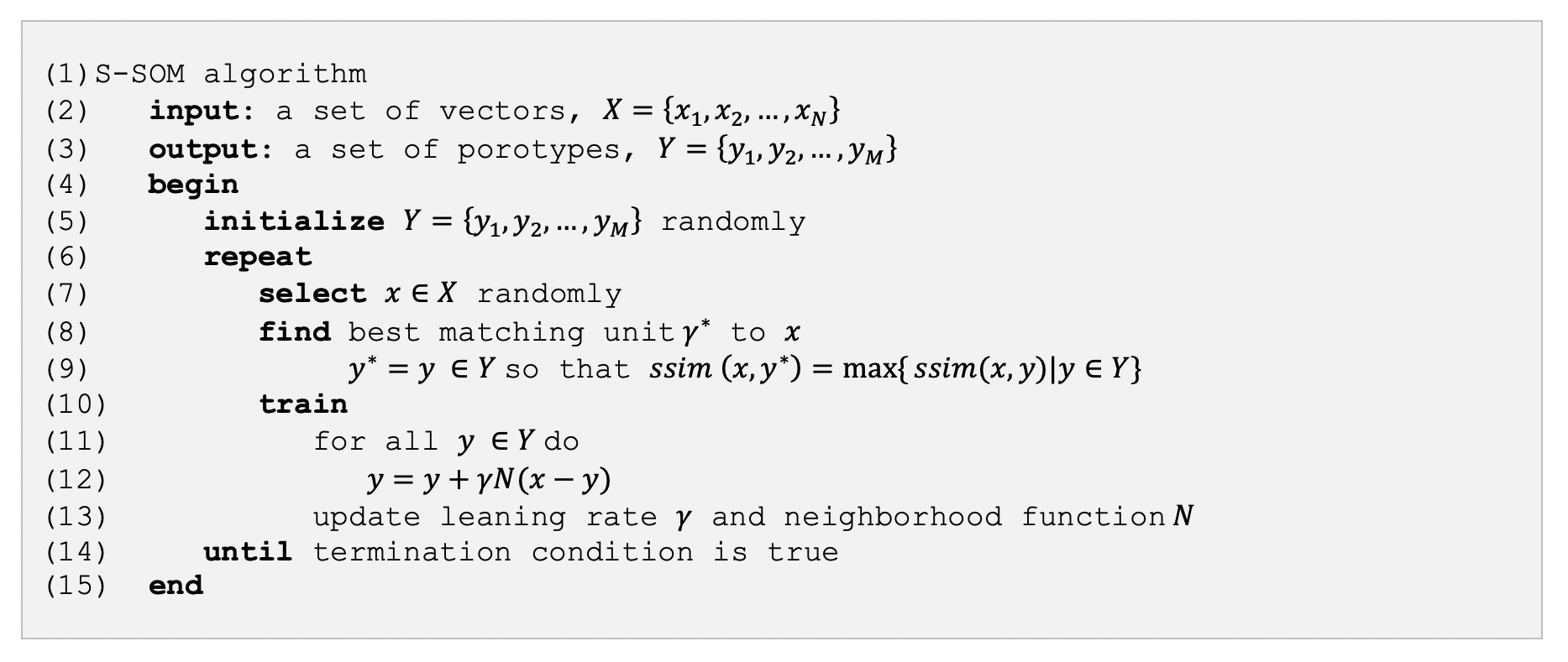
Our proposed S-SOM algorithm is shown in Fig. 1. It follows the procedure initially proposed by Kohonen (1982) and used in many application studies. An S-SOM starts with the configuration and initialization of SOM nodes and establishing the number of training iterations. The training consists of three main steps: selecting an input vector, finding the best matching unit for the input vector, then updating the weight vectors of SOM nodes by using parameters, i.e., learning rate and neighborhood function. The learning rate is a real number and decreases as the number of iteration steps increases. The difference between S-SOM and traditional SOM implementation is that we propose a new scheme for finding a BMU. In this scheme, we use a similarity index that can deal with structural data such as two-dimensional air pressure distribution instead of using ED to compare the similarity between vectors.
The new BMU search scheme is based on competition among SOM nodes so that a node with the highest S-SIM index to an input vector will be assigned as the BMU. The S-SIM was first introduced by Wang et al. (2004) to predict the perceived quality of digital television and cinematic pictures. The basic model was developed in the Laboratory for Image and Video Engineering at the University of Texas at Austin and further developed jointly with the laboratory for Computational Vision at New York University. The S-SIM index is designed to improve traditional methods such as the peak signal-to-noise ratio and mean squared error, i.e., methods based on ED, to detect similarities in “structural” signals such as images. The S-SIM formula is based on three comparison measurements between two vectors x, y, luminance (l), contrast (c), and structure (s).
Here, individual comparison functions are
Here, μx, μy are the average, σx, σy are the standard deviation, and , are the variance of vectors x, y, respectively; c1, c2, c3 are parameters to stabilize division with a weak denominator. Three components of S-SIM, i.e., “luminance”, “contrast”, and “structure”, represent human visual perception. The “luminance” measures the similarity in brightness values; “contrast” quantifies the similarity in illumination variability; and “structure” measures the correlation in spatial interdependencies between images (Wang and Bovik, 2009). To simplify the model, here we set and weights to reduce the original formula to
From the definition, S-SIM ranges from −1 to 1, where 1 indicates entirely similar, and vice versa. The S-SIM has been repeatedly shown to outperform ED significantly in terms of accuracy. Wang and Bovik (2009) pointed out that an S-SIM provides powerful, easy-to-use, and easy-to-understand alternatives to traditional ED for dealing with specific kinds of data that are spatially and temporally ordered. Recently, S-SIM has been attracting attention as a “new-generation” similarity metric in hydrological and meteorological studies (e.g., Mo et al., 2014; Han and Szunyogh, 2018).
3.1 Data and experiment settings
ERA-Interim (Dee et al., 2011) reanalysis daily mean sea-level pressure (MSLP) data for 1979–2019 over the Japan region (latitude 20 to 50∘ N and longitude 115 to 165∘ E; see Fig. 2) are used for demo simulations of S-SOM. The original MSLP data at a 0.75∘ resolution on a regular grid were interpolated to an equal-area scalable Earth-type grid at a spatial resolution of 100 km. This interpolation method has been commonly applied in high-latitude regions (Lynch et al., 2016; Gibson et al., 2017). The data are divided according to the four seasons: winter (December, January, February; DJF), spring (March, April, May; MAM), summer (June, July, August; JJA), autumn (September, October, November; SON).
The SOM grid topology consists of one-dimensional nodes. The training was carried out with 5000 iterations and with the learning rate start point at 0.01 (decreased exponentially to 0). The Gaussian function is used as the neighborhood function. A random initialization scheme was used. For completeness, we also train our SOMs with various configurations of n nodes = 4, 5, …, 20. The test for a larger number of nodes (greater than 100) was conducted, but the result showed the ineffectiveness of SOMs in clustering into a large number of classes. Together with S-SOM, ED- and COR-SOM experiments are also conducted for comparison. ED- and COR-SOM are SOM algorithms using the Euclidean distance and the Pearson correlation coefficient, respectively. For this test, the total of four (seasons) × 17 (node configurations) × 3 (S-SOM, COR-SOM, and ED-SOM) yields 204 runs that were conducted.
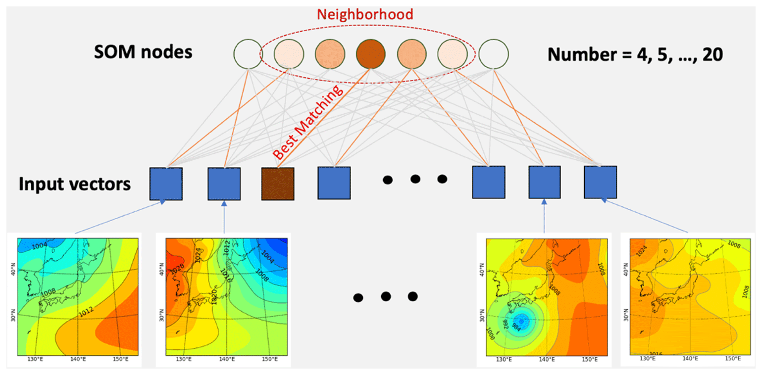
Figure 2Illustration of SOM configuration and simulation settings. Used data are daily (at 00:00 UTC) ERA-Interim sea-level pressure (from 1 January 1979 to 1 December 2019) divided into four seasons: winter (December–January–February), spring (March–April–May), summer (June–July–August), and autumn (September–October–November).
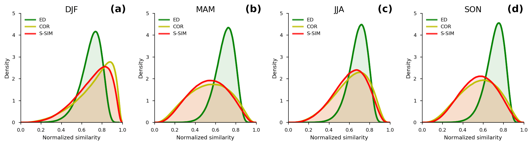
Figure 3Comparison of probability density distributions (PDDs) of normalized inter-sample similarity using the structural similarity (S-SIM), the Pearson correlation coefficient (COR), and the Euclidean distance (ED) for four-season data. The inter-sample similarity values indicate similarity (or difference) between all pairs. With a population size of N, one has (N−1)! values, as S-SIM, COR, and ED are symmetric measures. Values are normalized from 0 to 1, i.e., , with . The maximum similarity is 1, i.e., completely similar, and the minimum similarity is 0, i.e., the lowest similarity between a pair of data points. Note that the minimum similarity is dependent on a similarity measure and data (DJF, MAM, JJA, or SON) used.
3.2 Quality evaluation
We evaluate the performance of the SOMs, focusing on two different aspects. One is the capability as a clustering method, which we investigate by using silhouette analysis; the other is preserving the topology of input space, by analyzing topographical error. We select the evaluation metric based on its widespread use in clustering evaluation (silhouette analysis) and the SOM characteristics.
Silhouette refers to a method for the interpretation and validation of consistency within clusters of data. The technique provides a succinct graphical representation of how well each object has been classified (Rousseeuw, 1987). The silhouette value is a measure of how similar an object is to its cluster (cohesion) compared with other clusters (separation). The silhouette coefficient is calculated using the mean intra-cluster distance (a) and the mean nearest-cluster distance (b) for each sample. The silhouette coefficient for a given object is then defined as . The value ranges from −1 to +1, where a high value indicates that the object is well matched to its cluster and poorly matched to neighboring clusters. If most objects have high values, then the clustering configuration is appropriate. If many points have a low or negative value, then the clustering configuration may have too many or too few clusters. Silhouette coefficients near +1 indicate that the sample is far from the neighboring clusters. A value of 0 indicates that the object is on or very close to the decision boundary between two neighboring clusters. Negative values indicate that those samples might have been assigned to the wrong cluster. A critical goal of the SOM algorithm is to preserve the topological features of the input space. The topological error (TE) is defined as the average geometric distance between the winning and the second-best matching nodes in the SOM (Gibson et al., 2017). If the nodes are next to each other, we say that the topology has been preserved for this input; otherwise, it is counted as an error. The total number of errors divided by the total number of inputs gives the topographic error. TE measures how well the SOM models the structure of the input space. Primarily, it evaluates the local discontinuities in the mapping, i.e., . Here, di is the distance between the best matching and second-best matching units (SMUs) to an input vector xi; n is the total number of input vectors. The best value of TE is 1, meaning that the BMU and SMU are neighbors; i.e., SOM nodes are more topologically ordered (or more “self-organized”).
Table 1Statistical indices of normalized discrimination distributions.
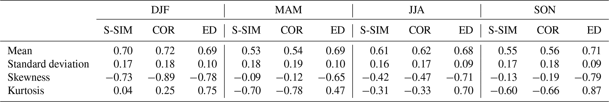
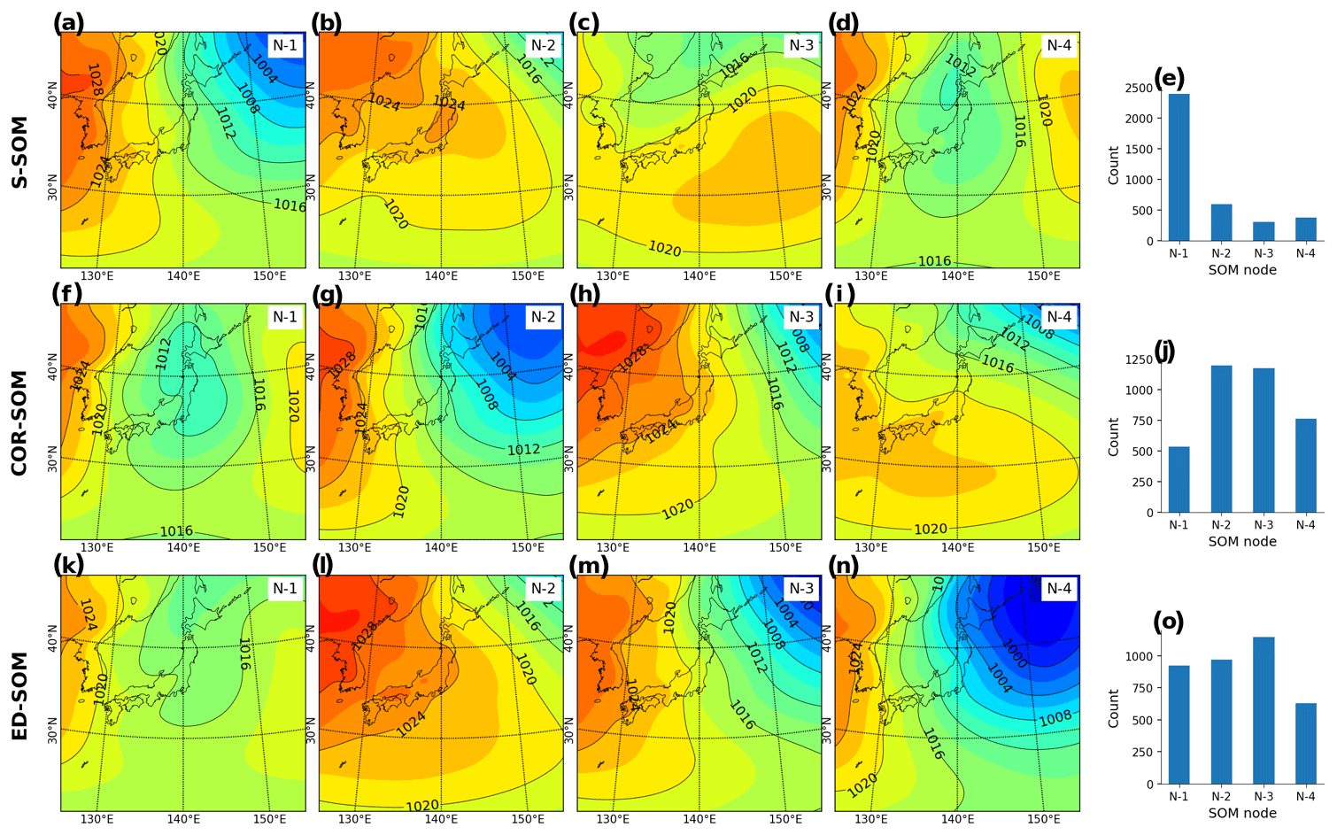
Figure 4Winter (DJF) MSLP pattern revealed by SOMs. Panels (a)–(d) show S-SOM patterns (with four nodes); panel (e) shows the number of daily MSLPs classified as nodes 1 to 4. Panels (f)–(i) show the same result but for COR-SOM; (k)–(o) for ED-SOM.
Before analyzing the SOM results, we examine how similarity indices, S-SIM, COR, and negative ED (as the similarity is inverse of distance metrics), distinguish SLP maps. The similarity index for each SLP data pair is calculated and normalized from 0 to 1, where 1 means precisely the same, and 0 means most different (indicating the value for the furthest pair). The probability density functions (PDFs) of these normalized similarities are shown in Fig. 3 for four datasets (DJF, MAM, JJA, and SON).
Two important points can be drawn from Fig. 3. First, the S-SIM and COR PDFs tend to spread over two tails, whereas those of ED appear to concentrate around their averages. The standard deviations of S-SIM and COR range 0.17–0.19, consistently higher than those of ED, which is 0.09–0.10 (Table 1). This result implies a higher ability of S-SIM and COR to recognize the inter-sample difference. Second, S-SIM and COR PDF shapes tend to vary, whereas ED's look identical for DJF, MAM, JJA, and SON. In other words, an S-SIM and COR can effectively recognize seasonal variability, but ED does not. The PDFs of ED have the mean at about 0.69 to 0.71, and skewness at about −0.65 to −0.79 among seasons. Meanwhile, the means of S-SIM and COR range widely from 0.53 to 0.72, and skewness from −0.09 to −0.89. In particular, for S-SIM and COR, the skewness is lower in DJF and JJA than in MAM and SON. In MAM and SON, the skewness is close to 0, meaning the PDFs are almost symmetric.
Regarding characterizing actual weather patterns, the PDFs of S-SIM and COR make more sense than those of ED. In DJF, Japan's weather is dominated by the winter-type air pressure (high in the west and low in the east), with few exceptions. This explains why the daily SLP in DJF looks similar most of the time; the PDFs' mean is higher than in other seasons; the skewness is deeply negative. The same weather trend is observed in the summer months (JJA). Meanwhile, in MAM and SON, which are transition periods between winter and summer, and vice versa, the weather variability is higher, and there are no dominant patterns during these times.
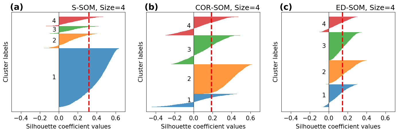
Figure 5Silhouette plots for S-, COR-, and ED-SOM clustering for winter months (DJF). Note that these are results from simulations with the SOM-node size of 4. The vertical dashed red lines in each plot indicate the silhouette score.
Next, we analyze the outcome of SOMs to ensure that the results are physically reasonable and match the common perception about seasonal weather patterns in Japan. Figure 4 shows the SLP patterns typed by SOMs (node number equal to 4) from the winter simulation (DJF). It is well known that the Japanese winter is characterized by the Siberian High, which develops over the Eurasian continent, and the Aleutian Low, which develops over the northern North Pacific. Prevailing northwesterly winds cause the advection of cold air from Siberia, bringing heavy snowfall to western Japan and sunny weather to the eastern side (http://www.data.jma.go.jp/gmd/cpd/longfcst/en/tourist_japan.html, last access: 6 January 2021). Such a dominant pattern is likely to be well detected by S-SOM (Fig. 4a), COR-SOM (Fig. 4g), and ED-SOM (Fig. 4n).
An interesting difference between SOMs is that S-SOM appears to estimate a more “ordered” clustering of nodes (Fig. 4e), characterized by a dominant node (N1) accompanied by non-dominant ones. Meanwhile, for COR-SOM and ED-SOM, the size of clusters is relatively identical, underlining the presence of more “flat” clustering (Fig. 4j, o). This result is consistently seen in other SOM-node configurations (i.e., node numbers greater than 4). “Ordered” clustering by S-SOM and “flat” clustering by COR- and ED-SOM are also recognized for JJA but to a lesser extent (see Fig. A3). The physical explanation for this is that two subperiods characterize the Japanese summer. The early subperiod is rainy, caused by the stationary Baiu front, where a warm maritime tropical air mass meets a cold polar maritime air mass. In the second subperiod, the North Pacific High extends northwestward around Japan, bringing hot and sunny conditions. The number of tropical cyclones passing the country peaks in August. Unlike DJF and JJA, MAM and SON are transition seasons, and the difference (i.e., “ordered” and “flat” clustering) is not apparent among SOMs.
Moreover, silhouette analysis shows that S-SOM and COR-SOM perform consistently better than ED-SOM in clustering SLP patterns. Figure 5 reveals two crucial points: one is the thickness of clusters (y axis) and the other is the silhouette coefficient value. As explained above, for DJF, S-SOM estimates one dominant winter-type SLP pattern combined with minor exception patterns. This is different from ED-SOM, which predicts more “flat” clusters with the same thickness. Thus, S-SOM clustering makes more sense than ED-SOM, and COR-SOM is somewhere in between them. The dominant Japanese winter-type pattern can be easily identified by looking at the S-SOM plot, but this is not the case with ED-SOM.
An important point here is that despite the “large” cluster, the silhouette values of S-SOM tend to be consistently higher than those of COR- and ED-SOM (Fig. 5). This result is highly counterintuitive because generally if the cluster is large, there is a higher possibility of data points being assigned to the wrong cluster. Also, Fig. 6 summarizes the silhouette score, compares three SOMs, and highlights two critical points: (i) S-SOM is consistently superior to ED-SOM for all seasons and all SOM-node configurations, demonstrating that S-SOM offers higher quality clustering than ED-SOM, which is consistent and independent of simulations; COR-SOM has comparable performance to S-SOM in MAM and SON but scores lower in DJF and partly in JJA; (ii) although not obvious, the scores of S-SOM and COR-SOM vary seasonally, whereas those of ED-SOM are identical among seasons. In particular, S-SOM scores the highest in weather types for DJF than for other seasons. Those are interesting results, noting that DJF in Japan is experientially known as the season most characterized by weather patterns in comparison to the other seasons.
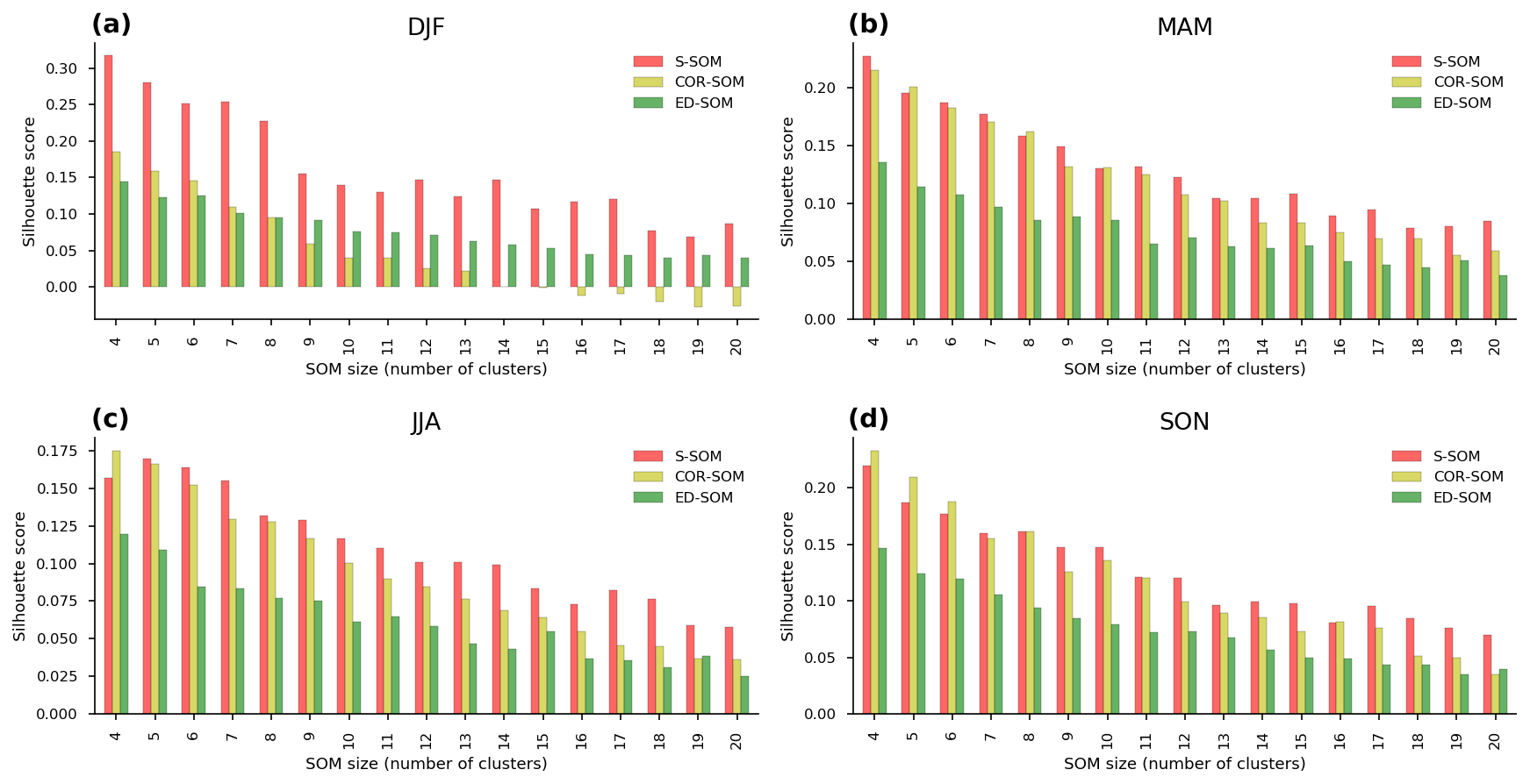
Figure 6Comparison of silhouette scores of S-, COR-, and ED-SOM for all SOM size configurations and four seasons, i.e., DJF, MAM, JJA, SON. In each plot, the x axis indicates a different SOM simulation (size configuration), and the y axis indicates silhouette score values.
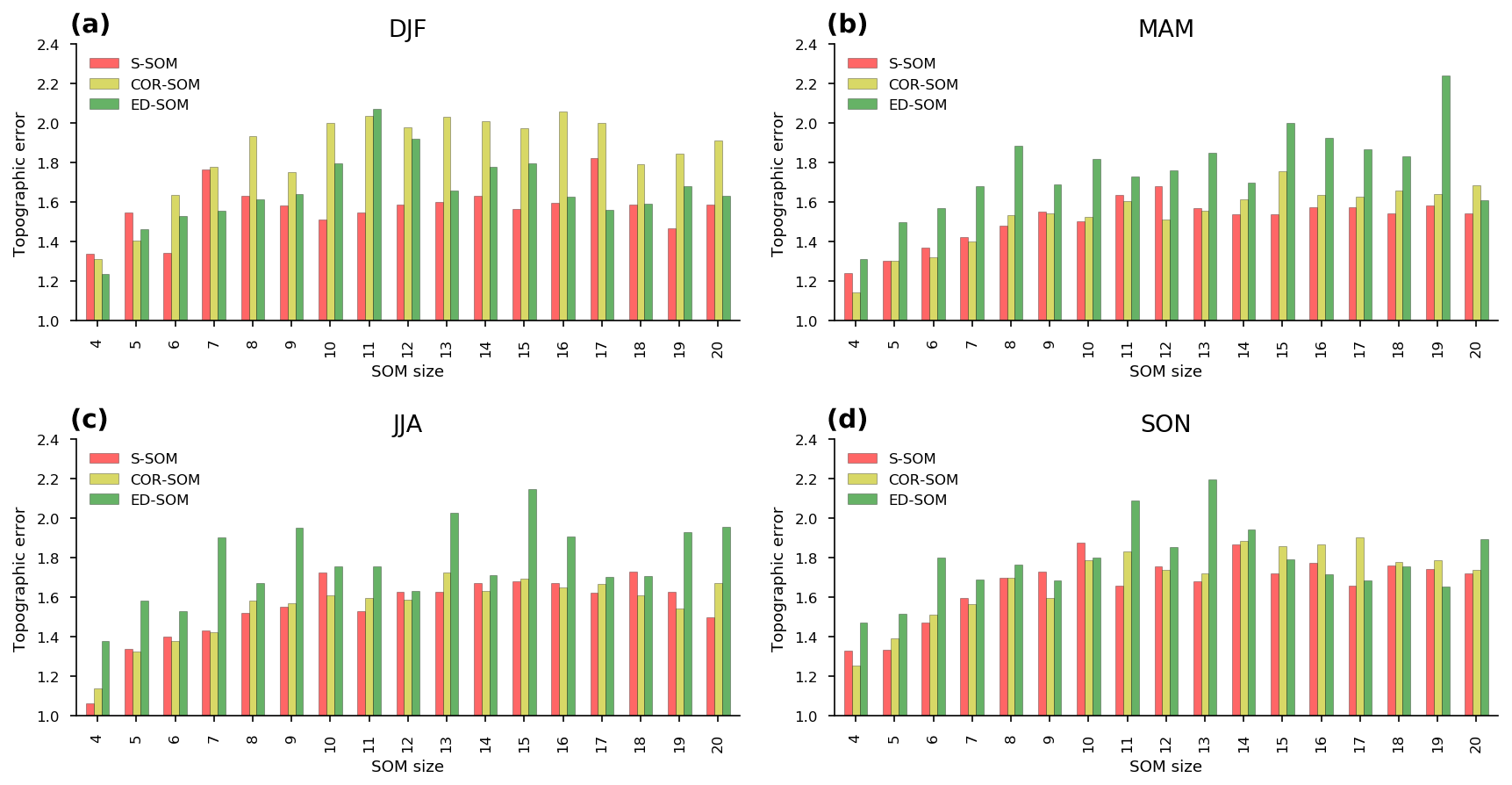
Figure 7Comparison of topographic errors of S-, COR-, and ED-SOM for all SOM size configurations and four seasons, i.e., DJF, MAM, JJA, SON. In each plot, the x axis indicates a different SOM simulation (size configuration), and the y axis indicates topographic errors.
As a measure of the topology preservation of SOM, TE indicates the lower error (higher topological preservation) of S-SOM, and partly COR-SOM, compared with ED-SOM (Fig. 7). Unlike with the silhouette score (Fig. 6), the difference in the TE values among SOMs is less noticeable and less consistent among SOM-node configurations and input data. A lower TE is always seen for MAM and JJA with almost all SOM size settings. However, for DJF, S-SOM has a higher TE, especially when it has a small size of 4 or 5. For SON, there is no apparent difference among SOMs. As TE is known to strongly depend on the neighborhood function (Gibson et al., 2017), the similarity detection scheme might have less impact. We also suggest that future studies are needed to clarify the topology preservation ability of SOMs with different similarity indices.
To confirm the above results, we have conducted additional simulations for wind vectors, a different type of data from SLP. As wind vectors consist of two components, i.e., zonal and meridional, we combine two components into one data array to feed the SOM models for each input vector. The test result shows that the S-SOM and COR-SOM have better performance over ED-SOM regarding both the silhouette score and the topographic error (see Figs. A8–A9 for reference). This result is consistent with that of SLP experiments.
Besides, the computational time of SOMs is calculated and shown in Fig. 8. ED-SOM needs 1–3 s to complete the jobs with node size ranging from 4–20. To do the same jobs, S-SOM needs 8–40 s, which are 10–15 times those of ED-SOM; COR-SOM needs 8–40 s or 8–13 times of ED-SOM. Though S-SOM needs more computational cost, it does not produce a critical issue as total computational time is small (less than 1 min) unlike the numerical weather prediction or climate change projection.
In this study, we developed a novel SOM algorithm (S-SOM) for synoptic weather typing. The novelty of S-SOM is the utilization of the structural similarity index (S-SIM) for searching for the best matching unit. The performance of S-SOM has been evaluated by a series of test simulations to cluster two-dimensional SLP and wind patterns over the Japan region.
Test results demonstrated the superior performance of S-SOM compared to the traditional ED-SOM (using the Euclidean distance). This result is consistent in all tests and SOM-node configurations in two respects: clustering quality in terms of the silhouette analysis and topological preservation in terms of the topographic error. The performance of S-SOM is higher than that of COR-SOM (using the Pearson correlation coefficient) but not as straightforward as compared to ED-SOM.
We highlight the effectiveness of using S-SOM, and partly COR-SOM rather than traditional ED-SOM, at least when spatial distributions feature input data. However, we emphasize that evaluation metrics other than the silhouette score and topographic errors should be used to robustify the results obtained in this study. Although this study did not assess the performance of S-SOM on time series, we believe that S-SOM can also be useful for temporally distributed data. The S-SOM performance with time series should be assessed in a further study. Moreover, although S-SOM has been developed primarily for climatology studies, it can also be used in other fields. We expect it will constitute the new standard SOM when dealing with “structural” input data.
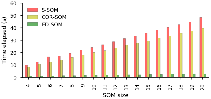
Figure 8Computational time of S-SOM, COR-SOM, and ED-SOM. The x axis indicates the SOM size configurations; the y axis represents the elapsed time needed to complete the jobs. These are the results of the DJF experiments. Each experiment has with 3669 input samples; the size of each sample is 65 × 72 pixels. The number of the SOM iteration steps is 5000.
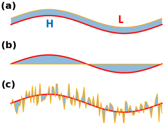
Figure A1Example faults with ED when distinguishing data that have a spatial and temporal correlation. Suppose we have two distributions represented by red and orange lines in each plot (a–c), where “H” and “L” are the locations of a high and a low, respectively. In panels (a)–(c), the red and orange lines have the same ED; meanwhile, if using the S-SIM index to compare the lines, one will have the highest S-SIM value in panel (a), followed by panel (c); the S-SIM values in both panels (a, c) are much higher than that in panel (b).
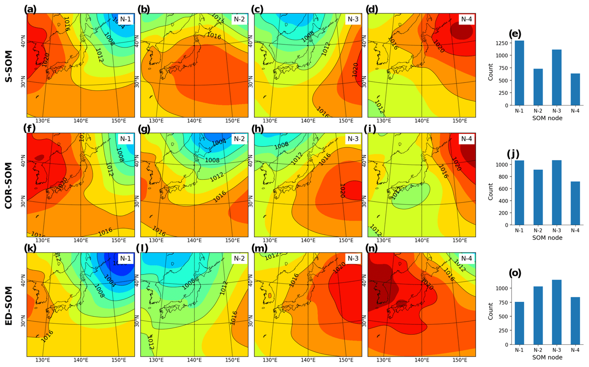
Figure A2Spring (MAM) MSLP pattern revealed by SOMs. Panels (a)–(d) show S-SOM patterns (with four nodes); panel (e) shows the number of daily MSLPs classified as nodes 1 to 4. Panels (f)–(i) show the same result but for COR-SOM; (k)–(o) for ED-SOM.
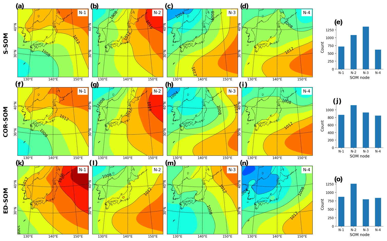
Figure A3Summer (JJA) MSLP pattern revealed by SOMs. Panels (a)–(d) show S-SOM patterns (with four nodes); panel (e) shows the number of daily MSLPs classified as nodes 1 to 4. Panels (f)–(i) show the same result but for COR-SOM; (k)–(o) for ED-SOM.
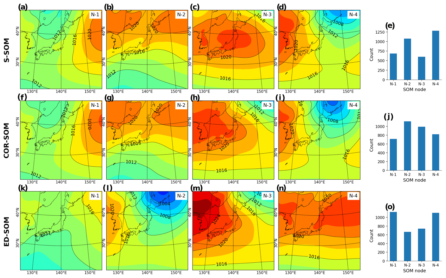
Figure A4Autumn (SON) MSLP pattern revealed by SOMs. Panels (a)–(d) show S-SOM patterns (with four nodes); panel (e) shows the number of daily MSLPs classified as nodes 1 to 4. Panels (f)–(i) show the same result but for COR-SOM; (k)–(o) for ED-SOM.
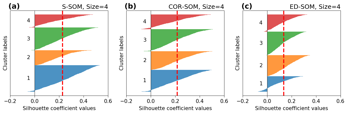
Figure A5Silhouette plot for S-, COR-, and ED-SOM clustering for spring months (MAM). Note that these are results from simulations with the SOM-node size of 4. The vertical dashed red lines in each plot indicate the silhouette score.
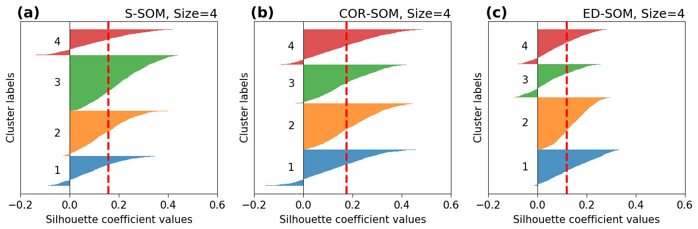
Figure A6Silhouette plot for S-, COR-, and ED-SOM clustering for summer months (JJA). Note that these are results from simulations with the SOM-node size of 4. The vertical dashed red lines in each plot indicate the silhouette score.
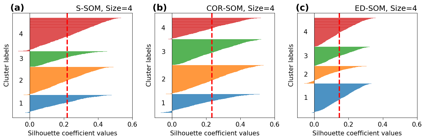
Figure A7Silhouette plot for S-, COR-, and ED-SOM clustering for autumn months (SON). Note that these are results from simulations with the SOM-node size of 4. The vertical dashed red lines in each plot indicate the silhouette score.
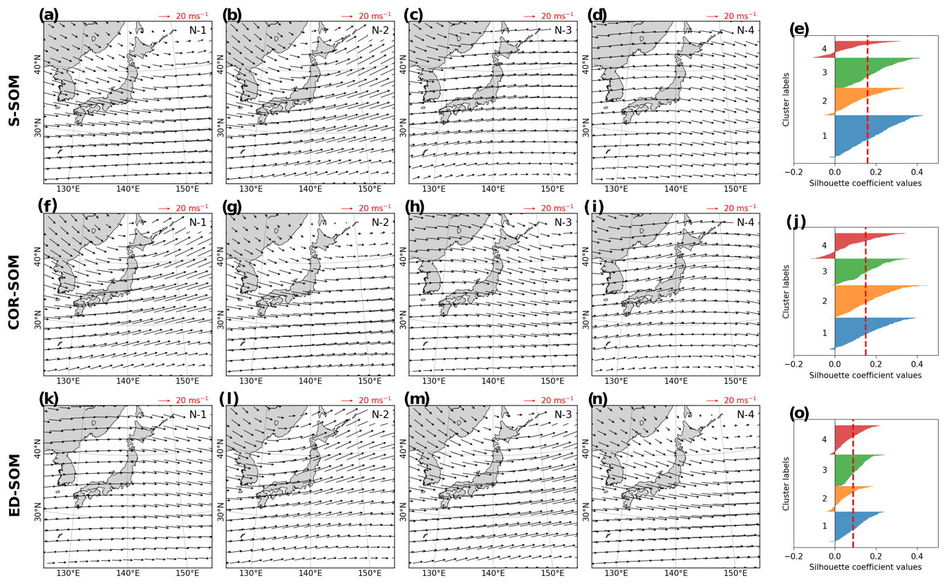
Figure A8Spatial patterns of the winter 500 hPa wind vector pattern revealed by SOMs with the size of 4. Panels (a)–(c) show the S-SOM results and panel (d) shows the silhouette analysis plot; panels (f)–(j) show the same results but for COR-SOM and (k)–(o) for ED-SOM. Input data are daily base data (at 00:00 UTC) winter months (DJF) from 2009 to 2019.
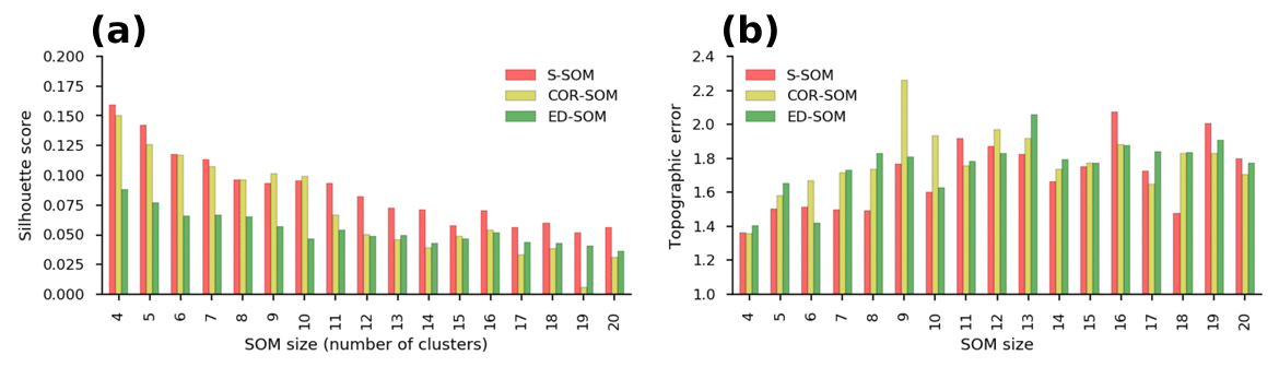
Figure A9Performance of S-, COR-, and ED-SOM for winter 500 hPa wind vector clustering. (a) The silhouette scores; (b) topographic errors of SOMs at different node sizes.
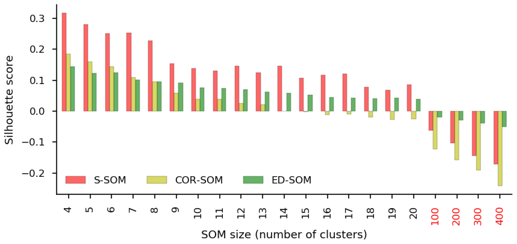
Figure A10Average silhouette scores of S-, COR-, and ED-SOM. The x axis indicates the SOM size configurations. The y axis shows the silhouette score, which ranges from −1 to 1. For a given sample, the perfect cluster assignment has the value of 1, and negative values indicate the wrong cluster assignment for the sample.
The exact version of the model used to produce the results used in this paper is archived on Zenodo (https://doi.org/10.5281/zenodo.4437954, Doan, 2021), as are input data and scripts to run the model and make the plots for all the simulations presented in this paper.
QVD designed the model and developed the model code. HK and TS helped to design the test experiments. HK, TS, and FC helped to analyze the results. QVD prepared the manuscript with contributions from all co-authors.
The authors declare that they have no conflict of interest.
This research was funded by the Environment Research and Technology Development Fund (JPMEERF20192005) of the Environmental Restoration and Conservation Agency of Japan. Quang-Van Doan is grateful for support from JSPS KAKENHI grant nos. JP20K13258 and JP19H01155. Fei Chen is grateful for support from the Water System Program at the National Center for Atmospheric Research (NCAR), NASA IDS grant no. 80NSSC20K1262, USDA NIFA grant nos. 2015-67003-23508 and 2015-67003-23460, NOAA grant no. NA18OAR4590398, and NSF grant no. 1739705.
This paper was edited by David Topping and reviewed by two anonymous referees.
Alexander, L. V., Uotila, P., Nicholls, N., and Lynch, A.: A new daily pressure dataset for Australia and its application to the assessment of changes in synoptic patterns during the last century, J. Climate, 23, 1111–1126, 2010.
Borah, N., Sahai, A., Chattopadhyay, R., Joseph, S., Abhilash, S., and Goswami, B.: A self-organizing map–based ensemble forecast system for extended range prediction of active/break cycles of Indian summer monsoon, J. Geophys. Res.-Atmos., 118, 9022–9034, 2013.
Chang, L.-C., Shen, H.-Y., and Chang, F.-J.: Regional flood inundation nowcast using hybrid SOM and dynamic neural networks, J. Hydrol., 519, 476–489, 2014.
Dee, D. P., Uppala, S. M., Simmons, A. J., Berrisford, P., Poli, P., Kobayashi, S., Andrae, U., Balmaseda, M. A., Balsamo, G., Bauer, P., Bechtold, P., Beljaars, A. C. M., van de Berg, I., Biblot, J., Bormann, N., Delsol, C., Dragani, R., Fuentes, M., Greer, A. J., Haimberger, L., Healy, S. B., Hersbach, H., Holm, E. V., Isaksen, L., Kallberg, P., Kohler, M., Matricardi, M., McNally, A. P., Mong-Sanz, B. M., Morcette, J.-J., Park, B.-K., Peubey, C., de Rosnay, P., Tavolato, C., Thepaut, J. N., and Vitart, F.: The ERA-Interim reanalysis: Configuration and performance of the data assimilation system, Q. J. Roy. Meteorol. Soc., 137, 553–597, https://doi.org/10.1002/qj.828, 2011.
Doan, Q. V.: S-SOM v1.0: A structural self-organizing map algorithm for weather typing (Version V1), Zenodo, https://doi.org/10.5281/zenodo.4437954, 2021.
Gibson, P. B., Perkins-Kirkpatrick, S. E., and Renwick, J. A.: Projected changes in synoptic weather patterns over New Zealand examined through self-organizing maps, Int. J. Climatol., 36, 3934–3948, 2016.
Gibson, P. B., Perkins-Kirkpatrick, S. E., Uotila, P., Pepler, A. S., and Alexander, L. V.: On the use of self-organizing maps for studying climate extremes, J. Geophys. Res.-Atmos., 122, 3891–3903, 2017.
Han, F. and Szunyogh, I.: A Technique for the Verification of Precipitation Forecasts and Its Application to a Problem of Predictability, Mon. Weather Rev., 146, 1303–1318, 2018.
Horton, D. E., Johnson, N. C., Singh, D., Swain, D. L., Rajaratnam, B., and Diffenbaugh, N. S.: Contribution of changes in atmospheric circulation patterns to extreme temperature trends, Nature, 522, 465–469, 2015.
Kaski, S.: Data Exploration Using Self-Organizing Maps. Acta Polytechnica Scandinavica, Mathematics, Computing and Management in Engineering Series No. 82, Finnish Academy of Technology, Espoo, Finland, ISBN 978-952-5148-13-8, 1997.
Kohonen, T.: A simple paradigm for the self-organized formation of structured feature maps, in Competition and cooperation in neural nets, Springer, 248–266, 1982.
Lagerquist, R., Flannigan, M. D., Wang, X., and Marshall, G. A.: Automated prediction of extreme fire weather from synoptic patterns in northern Alberta, Canada, Can. J. For. Res., 47, 1175–1183, 2017.
Lennard, C. and Hegerl, G.: Relating changes in synoptic circulation to the surface rainfall response using self-organising maps, Clim. Dynam., 44, 861–879, 2015.
Luong, T. M., Dasari, H. P., and Hoteit, I.: Extreme precipitation events are becoming less frequent but more intense over Jeddah, Saudi Arabia. Are shifting weather regimes the cause?, Atmos. Sci. Lett., 21, e981, https://doi.org/10.1002/asl.981, 2020.
Lynch, A. H., Serreze, M. C., Cassano, E. N., Crawford, A. D., and Stroeve, J.: Linkages between Arctic summer circulation regimes and regional sea ice anomalies, J. Geophys. Res.-Atmos., 121, 7868–7880, 2016.
Mo, R., Ye, C., and Whitfield, P. H.: Application potential of four nontraditional similarity metrics in hydrometeorology, J. Hydrometeorol., 15, 1862–1880, 2014.
Nguyen-Le, D. and Yamada, T. J.: Using weather pattern recognition to classify and predict summertime heavy rainfall occurrence over the Upper Nan river basin, northwestern Thailand, Weather Forecast., 34, 345–360, 2019.
Nguyen-Le, D., Yamada, T. J., and Tran-Anh, D.: Classification and forecast of heavy rainfall in northern Kyushu during Baiu season using weather pattern recognition, Atmos. Sci. Lett., 18, 324–329, 2017.
Ohba, M. and Sugimoto, S.: Differences in climate change impacts between weather patterns: possible effects on spatial heterogeneous changes in future extreme rainfall, Clim. Dynam., 52, 4177–4191, 2019.
Ohba, M., Kadokura, S., and Nohara, D.: Medium-range probabilistic forecasts of wind power generation and ramps in Japan based on a hybrid ensemble, Atmosphere, 9, 423, https://doi.org/10.3390/atmos9110423, 2018.
Rousseeuw, P. J.: Silhouettes: a graphical aid to the interpretation and validation of cluster analysis, J. Comput. Appl. Math., 20, 53–65, 1987.
Shah-Hosseini, H.: Binary tree time adaptive self-organizing map, Neurocomputing, 74, 1823–1839, 2011.
Shah-Hosseini, H. and Safabakhsh, R.: TASOM: a new time adaptive self-organizing map, IEEE T. Syst. Man. Cy. B, 33, 271–282, 2003.
Sheridan, S. C. and Lee, C. C.: The self-organizing map in synoptic climatological research, Prog. Phys. Geogr., 35, 109–119, 2011.
Swales, D., Alexander, M., and Hughes, M.: Examining moisture pathways and extreme precipitation in the US Intermountain West using self-organizing maps, Geophys. Res. Lett., 43, 1727–1735, 2016.
Wang, Z. and Bovik, A. C.: Mean squared error: Love it or leave it? A new look at signal fidelity measures, IEEE Signal Process. Mag., 26, 98–117, 2009.
Wang, Z., Bovik, A. C., Sheikh, H. R., and Simoncelli, E. P.: Image quality assessment: from error visibility to structural similarity, IEEE Trans. Image Process., 13, 600–612, 2004.