Effects of coupling a stochastic convective parameterization with the Zhang–McFarlane scheme on precipitation simulation in the DOE E3SMv1.0 atmosphere model

A stochastic deep convection parameterization is implemented into the US Department of Energy (DOE) Energy Exascale Earth System Model (E3SM) Atmosphere Model version 1.0 (EAMv1). This study evaluates its performance in simulating precipitation. Compared to the default model, the probability distribution function (PDF) of rainfall intensity in the new simulation is greatly improved. The well-known problem of “too much light rain and too little heavy rain” is alleviated, especially over the tropics. As a result, the contribution from different rain rates to the total precipitation amount is shifted toward heavier rain. The less frequent occurrence of convection contributes to suppressed light rain, while more intense large-scale and convective precipitation contributes to enhanced heavy total rain. The synoptic and intraseasonal variabilities of precipitation are enhanced as well to be closer to observations. The sensitivity of the rainfall intensity PDF to the model vertical resolution is examined. The relationship between precipitation and dilute convective available potential energy in the stochastic simulation agrees better with that in the Atmospheric Radiation Measurement (ARM) observations compared with the standard model simulation. The annual mean precipitation is largely unchanged with the use of the stochastic scheme except over the tropical western Pacific, where a moderate increase in precipitation represents a slight improvement. The responses of precipitation and its extremes to climate warming are similar with or without the stochastic deep convection scheme.

1 Introduction

Precipitation plays a vital role in the Earth's climate: the latent heat released during precipitation formation is a major energy source that drives the atmospheric circulation, and precipitation is an important part of the Earth's hydrological cycle. The accurate simulation of precipitation in global climate models (GCMs) is of great scientific and societal interest. However, GCMs used for current climate simulation and future projections suffer from many biases in the global distribution, frequency and intensity of simulated precipitation (Dai, 2006), which have negatively impacted the model's fidelity. Rainfall in nature is tightly associated with many complex dynamic and physical processes in the atmosphere, including large-scale circulation, convection, cloud microphysics and planetary boundary layer (PBL) processes. The deficiencies in representing these processes in GCMs are prime culprits for errors in simulated rainfall (Watson et al., 2017).

Among the physical processes in GCMs, the parameterization of convection is responsible for some well-known biases: the double Intertropical Convergence Zone (Zhang and Wang, 2006; Zhang et al., 2019), synoptic and intraseasonal variabilities in the tropics that are too weak (Zhang and Mu, 2005a; Watson et al., 2017), the wrong diurnal cycle of rainfall (Xie et al., 2019), and “too much light rain and too little heavy rain” (Dai, 2006; Zhang and Mu, 2005b; O'Gorman and Schneider, 2009) to name a few. The conventional deterministic convective parameterization in GCMs represents the ensemble effects of subgrid-scale convective clouds in a model grid box on resolved scale variables. However, in reality, a given grid-scale state may lead to different realizations of subgrid-scale convection (Davies et al., 2013; Peters et al., 2013) rather than to a single “ensemble mean” response. For instance, two model grid boxes, both in a similar convective equilibrium state, can have different numbers and/or sizes of convective clouds due to stochasticity (Cohen and Craig, 2006). This stochasticity will appear more frequently as the model grid box size becomes smaller (Jones and Randall, 2011). Not including stochasticity in convective schemes has been suggested to be at least partly responsible for the weak intraseasonal variability and “too much light rain and too little heavy rain” in GCMs (Lin and Neelin, 2000; Wang et al., 2016; Watson et al., 2017; Peters et al., 2017).

As suggested in Palmer (2001, 2012), more realistic statistics of the impacts of subgrid convective clouds should be derived by simulating them as random samples from probability distributions conditioned on the grid-scale state so that the influences of different individual realizations are introduced in the convection parameterization. In this regard, much effort in the past 2 decades has been made to develop stochastic convection schemes (e.g., Lin and Neelin, 2000, 2002; Plant and Craig, 2008; Khouider et al., 2010; Sakradzija et al., 2015). Among these schemes, Plant and Craig (2008) (PC08 hereafter) developed a stochastic deep convection parameterization under a framework based on statistical mechanics (Cohen and Craig, 2006; Craig and Cohen, 2006) for noninteracting convective clouds in statistical equilibrium using cloud-resolving model (CRM) simulations. This scheme was applied to numerical weather prediction (NWP) models and to a GCM in an aquaplanet setting, resulting in some substantial improvements in precipitation simulation (Groenemeijer and Craig, 2012; Keane et al., 2014, 2016).

Wang et al. (2016) incorporated the PC08 stochastic deep convection scheme into the Zhang–McFarlane (ZM) deterministic deep convection scheme (Zhang and McFarlane, 1995) in the National Center for Atmospheric Research (NCAR) Community Atmosphere Model version 5 (CAM5). They found that the introduction of the stochastic scheme improved the simulation of precipitation intensity and intraseasonal variability over the tropics in CAM5 (Wang and Zhang, 2016; Wang et al., 2017).

In this study, we implement the PC08 stochastic deep convection parameterization scheme into the DOE Energy Exascale Earth System Model (E3SM) (Golaz et al., 2019) Atmosphere Model version 1.0 (EAMv1) (Rasch et al., 2019; Xie et al., 2018) and examine its effect on precipitation simulation. The EAMv1 is branched out from CAM5, and it thus inherits many model deficiencies from CAM5 as well. Many modifications in physics parameterizations have been made compared to CAM5 (Rasch et al., 2019; Xie et al., 2018). However, some model biases, such as weak precipitation intensity, persist (Xie et al., 2019). Thus, besides the precipitation metrics explored in our previous studies (Wang et al., 2016, 2017; Wang and Zhang, 2016), this study will evaluate precipitation simulation with more systematical metrics. In addition, the responses of precipitation and its extremes to climate warming with the stochastic deep convection scheme will be investigated.

The organization of the paper is as follows. Section 2 presents the parameterization, model, experimental design and evaluation data. Section 3 describes results, including variability, frequency, intensity, amounts, duration, mean state, and the responses of precipitation and its extremes to climate warming. The sensitivity of the rainfall intensity PDF to vertical resolution and underlying mechanisms are also presented in this section. A summary is given in Sect. 4.

2 Parameterization, model, experimental design and evaluation data

2.1 Stochastic deep convection parameterization

The stochastic convective parameterization scheme of PC08 is modified for climate models when incorporating it into the ZM deterministic deep convection scheme. The most essential part of the PC08 scheme involves two probability distributions. One is the probability distribution of mass flux of a cloud; it follows the exponential distribution

$$\begin{array}{}\text{(1)}& p\left(m\right)\mathrm{d}m={\displaystyle \frac{\mathrm{1}}{\langle m\rangle }}{e}^{-m/\langle m\rangle }\mathrm{d}m,\end{array}$$

where 〈m〉 is the mean mass flux of a cloud and is a preset tuning parameter. The integral of the probability density over all values of mass flux is 1, i.e., the probability of 1 that every cloud has a mass flux between zero and infinity. The other is the probability of triggering n clouds for a given cloud mass flux in the range between m and m+dm at a given GCM grid box and time step; it is drawn from a Poisson distribution:

$$\begin{array}{}\text{(2)}& P_{\langle N\rangle }\left(n\right)={\displaystyle \frac{\langle N{\rangle }^n{e}^{-\langle N\rangle }}{n\mathrm{!}}}\text{ for }n=\mathrm{0},\mathrm{1},\mathrm{2},\mathrm{3}\mathrm{\dots },\end{array}$$

where 〈N〉 is the ensemble mean number of convective clouds in the grid box. Here the sum of the probabilities over all n must equal 1, i.e., the probability of 1 that some number between zero and an infinite number of clouds will be triggered with mass flux in this interval. Thus, the average number of clouds with mass flux between m and m+dm, $d\overline{n}\left(m\right)$, is

$$\begin{array}{}\text{(3)}& \mathrm{d}\overline{n}\left(m\right)=\langle N\rangle p\left(m\right)\mathrm{d}m={\displaystyle \frac{\langle N\rangle }{\langle m\rangle }}{e}^{-m/\langle m\rangle }\mathrm{d}m.\end{array}$$

From Eqs. (2) and (3), it follows then that for small $\mathrm{d}\overline{n}\left(m\right)$ the probability of launching one convective cloud with mass flux between m and m+dm is given by

$$\begin{array}{}\text{(4)}& p_{\mathrm{d}\overline{n}\left(m\right)}\left(n=\mathrm{1}\right)={\displaystyle \frac{\langle N\rangle }{\langle m\rangle }}{e}^{-m/\langle m\rangle }\mathrm{d}m.\end{array}$$

Note that Eq. (4) is not a probability density function, but rather the probability of triggering one cloud for a given cloud mass flux interval (m, m+dm), knowing that the average number of clouds within this mass flux interval is $\mathrm{d}\overline{n}\left(m\right)$. $\langle N\rangle =\langle M\rangle /\langle m\rangle$, where 〈M〉 is the ensemble mean total cloud mass flux given by the closure based on the convective quasi-equilibrium assumption in the ZM deterministic parameterization. For each mass flux bin, whether to launch a cloud is determined by comparing the probability $\frac{\mathrm{1}}{\langle m\rangle }{e}^{-\frac{m}{\langle m\rangle }}\mathrm{d}m$ with a random number uniformly generated between zero and 1. Then, the sum of mass fluxes generated this way is multiplied by the factor 〈N〉 to rescale it to the mass flux of all clouds. The product of the total mass flux and the temperature and moisture tendencies from the bulk plume model gives the final temperature and moisture tendencies by the subgrid convective clouds.

There are two modifications to the original implementation in the NCAR CAM5. One is the update frequency of random numbers, which, unlike the update frequency of once a day in Wang et al. (2016), is updated every 3 d in consideration of computational resources due to finer vertical and horizontal resolutions in the EAMv1 (see Sect. 2.2). For the same reason, the spatial averaging of input quantities (i.e., vertical profiles of temperature and moisture) to the closure over neighboring grid points used in the original design of PC08 is not performed because it leads to an excessive communication load. One can argue that at a horizontal model resolution of about 110 km in EAMv1, convective quasi-equilibrium approximately holds over some timescale, although at individual model time steps it does not. Thus, although spatial averaging is not applied, the temporal trailing averaging over 3 h at each time step is retained in the scheme. Other modifications to the PC08 scheme for incorporation into the ZM scheme in climate models (Wang et al., 2016) are retained. These include the following.

1. The temporally averaged quantities are used to calculate the ensemble mean cloud mass flux (〈M〉), which is determined by the ZM scheme. The unsmoothed grid point quantities are still used in the trigger function and the cloud model.

2. The root mean squared cloud radius information originally used in PC08 is not needed in our implementation because the ZM scheme does not use cloud radius.

3. The ensemble mean mass flux of a cloud 〈m〉 is set to 1×10⁷ kg s⁻¹ following Groenemeijer and Craig (2012).

4. The cloud life cycle effect with a factor $\mathrm{d}t/T$ (dt is the model time step and T is the constant lifetime parameter) in PC08 is not taken into account because the ZM deterministic parameterization does not consider the life cycle of convection.

2.2 EAMv1 model

The standard configuration of the DOE EAMv1 uses a spectral element dynamical core at a 110 km horizontal resolution on a cubed sphere geometry and a vertical resolution of 72 layers from the surface to 60 km (10 Pa) (Rasch et al., 2019; Xie et al., 2018). The treatments of PBL turbulence, shallow convection and cloud macrophysics are unified with a simplified third-order turbulence closure parameterization, CLUBB (Cloud Layers Unified by Binormals; Golaz et al., 2002; Larson and Golaz, 2005). The deep convection is represented by the ZM scheme. The Morrison and Gettelman (2008) (MG) microphysics scheme is updated to MG2 (Gettelman et al., 2015) with the prediction of rain and changes to ice nucleation and ice microphysics (Wang et al., 2014). A four-mode version of the modal aerosol module (MAM4) (Liu et al., 2016) is used with improvements to aerosol resuspension, aerosol nucleation, scavenging, convective transport and sea spray emissions for including the contribution of marine ecosystems to organic matter (Rasch et al., 2019). A linearized ozone chemistry module (Hsu and Prather, 2009; McLinden et al., 2000) is used to represent stratospheric ozone and its radiative impacts in the stratosphere. Other modifications for model tuning are provided in detail in Xie et al. (2018).

Table 1 List of simulations.

^a Atmosphere-only simulations using fully prognostic atmosphere and land models with prescribed, seasonally varying climatological present-day sea surface temperatures (SSTs) and sea ice extent, recycled yearly.
^b For simulating a warmer world, the atmosphere-only simulations are subjected to a composite SST warming pattern derived from the Coupled Model Intercomparison Project Phase 3 (CMIP3) coupled models.

2.3 Experimental design

Six Atmospheric Model Intercomparison Project (AMIP) types of simulations are conducted. Four 6-year simulations are forced by prescribed, seasonally varying climatological present-day sea surface temperatures (SSTs) and sea ice extent, recycled yearly (Stone et al., 2018): two with the default deterministic ZM scheme but having 72 and 30 vertical levels (referred to as EAMv1 and EAMv1–30L, respectively) and the other two with the stochastic deep convection scheme (referred to as STOCH and STOCH–30L). The simulations with 30 vertical levels are conducted to facilitate the comparison with Wang et al. (2016), in which the vertical resolution of CAM5 is 30 levels (see Sect. 3.3). To explore the responses of precipitation and its extremes to climate warming, similar to EAMv1 and STOCH runs, two 3-year simulations in a warmer climate are conducted, in which a composite SST warming pattern derived from the Coupled Model Intercomparison Project Phase 3 (CMIP3) coupled models (referred to as EAMv1–4K and STOCH–4K, respectively) is imposed for the boundary condition of the atmosphere. Following Webb et al. (2017), it is a normalized multi-model mean of the sea surface temperature response pattern from 13 CMIP3 atmosphere–ocean general circulation models, representing the change in SST between years 0–20 and 140–160, the time of CO₂ quadrupling in the 1 % runs. Before calculating the multi-model ensemble mean, the SST response of each model was divided by its global mean and multiplied by 4 K. This guarantees that the pattern information from all models is weighted equally and that the global mean SST forcing is +4 K warming. The first year in all simulations is discarded as a spin-up. Information for all experiments is summarized in Table 1.

2.4 Evaluation data

For model evaluation, the following datasets are used: the Clouds and the Earth's Radiant Energy System Energy Balanced and Filled (CERES-EBAF) (Loeb et al., 2009) for evaluation of shortwave and longwave cloud radiative forcing; the European Centre for Medium-Range Weather Forecasts Interim Reanalysis (ERAI) (Simmons et al., 2007) for sea level pressure, zonal wind, relative humidity, specific humidity and temperature; the European Remote Sensing Satellite Scatterometer (ERS) (Bentamy et al., 1999) for surface wind stress; and the Willmott–Matsuura (Willmott) (Willmott and Matsuura, 1995) data for land surface air temperature.

The rainfall mean state is evaluated against the Global Precipitation Climatology Project (GPCP) monthly product (version 2.1) at a resolution of 2.5^∘ (Adler et al., 2003; Huffman et al., 2009), while a daily estimate of GPCP version 1.2 at 1^∘ horizontal resolution (GPCP 1DD) (Huffman et al., 2001, 2012) is used for the evaluation of precipitation amount distribution. In addition to GPCP, the Xie–Arkin pentad observations at 2.5^∘ resolution (Xie and Arkin, 1996) and the Tropical Rainfall Measuring Mission 3B42 version 7 (TRMM) daily observations at a resolution of 0.25^∘ over (50^∘ S, 50^∘ N) (Huffman et al., 2007) are applied to evaluate the precipitation variance. The TRMM data are also used in the PDF of rainfall intensity and the rainfall amount distribution. To estimate the uncertainty in the PDF of precipitation intensity in observations, additional daily rainfall products are used. These include TAPEER v1.5, GSMaP-NRT-gauge v6.0, PERSIANN CDR v1, CMORPH v1.0 CRT from the Frequent Rainfall Observation on GridS (FROGS) database (Roca et al., 2019) and Global Precipitation Measurement (GPM) IMERG v06b (Huffman et al., 2017). For the rainfall duration evaluation, the TRMM 3B42 v7 3-hourly data are used. To make the comparison consistent between observations and model simulations, the model data with the same output frequency as that in the corresponding observations and/or reanalysis data are used, and all observations and/or reanalysis data are regridded to the same 1^∘ lat–long grids as EAMv1. The US Department of Energy Atmospheric Radiation Measurement (ARM) multiyear observations for daily precipitation and dilute convective available potential energy (CAPE) over the Southern Great Plains (SGP) site for the time period of 2004–2018 (Xie et al., 2004) and the Green Ocean Amazon (GOAmazon) field campaign (Martin et al., 2016) site for 2014–2015 (Tang et al., 2016) are used to evaluate the simulated CAPE vs. precipitation relationship.

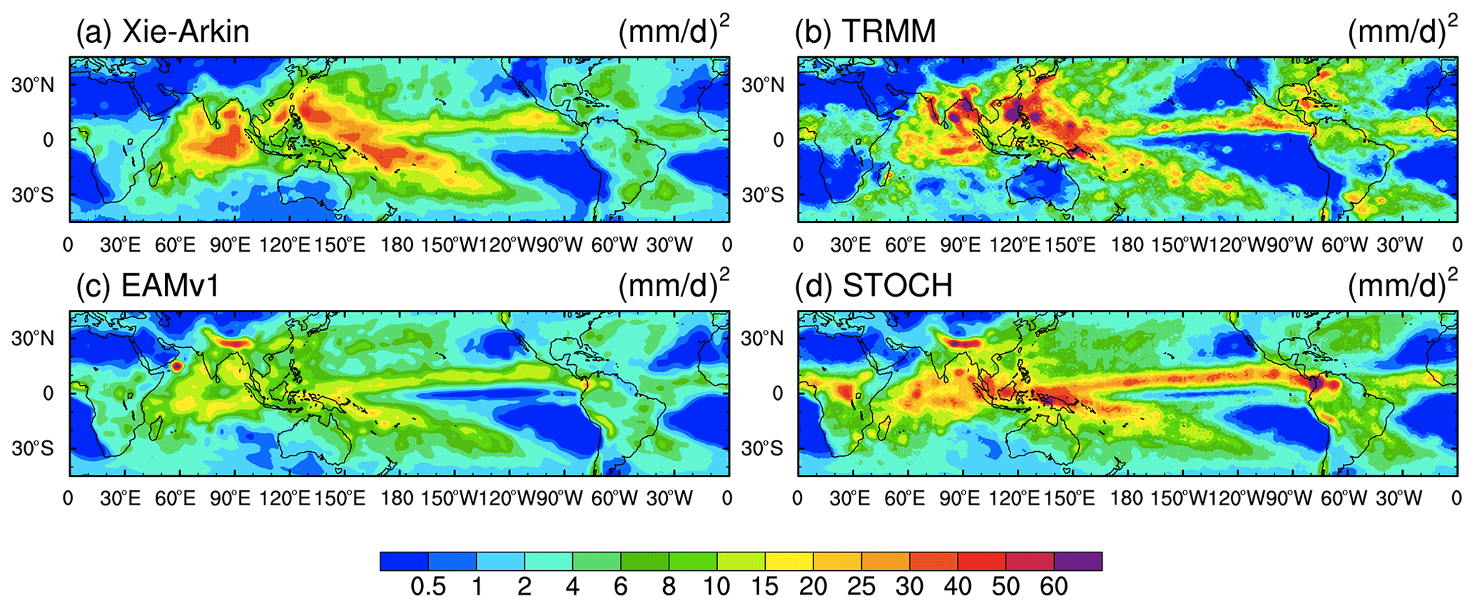
Figure 1 Spatial distributions of the 20–80 d variance of rainfall from (a) the Xie–Arkin observations, (b) TRMM, (c) EAMv1 and (d) STOCH (units: mm² d⁻²).

3 Results

3.1 Intraseasonal and synoptic variability

The simulated variability of precipitation is an important aspect of model performance. Here we focus on intraseasonal and synoptic-scale variability. The intraseasonal variability associated with the Madden–Julian oscillation (MJO) is problematic in many GCMs (Jiang et al., 2015; Zhang and Mu, 2005a). Figure 1 shows the tropical distribution of the 20–80 d intraseasonal variance for the total precipitation in observations and simulations. The variance is obtained with a Lanczos band-pass filter at each grid point. Both Xie–Arkin and TRMM observations show large variance in the Indian Ocean and western Pacific as well as in the ITCZ and the South Pacific Convergence Zone (SPCZ). The intraseasonal variance in EAMv1 is much weaker, as in many other GCMs. Similar to the results in Wang et al. (2016), the STOCH run with the stochastic deep convection scheme has significantly enhanced intraseasonal variance in these regions, making it much more comparable to observations, although there is excessive precipitation variance over central Africa, the Himalayas, the Maritime Continent and the region near the Colombian coast. Compared with the EAMv1 run, the STOCH run has more small-scale noise in the spatial structure of the precipitation variability.

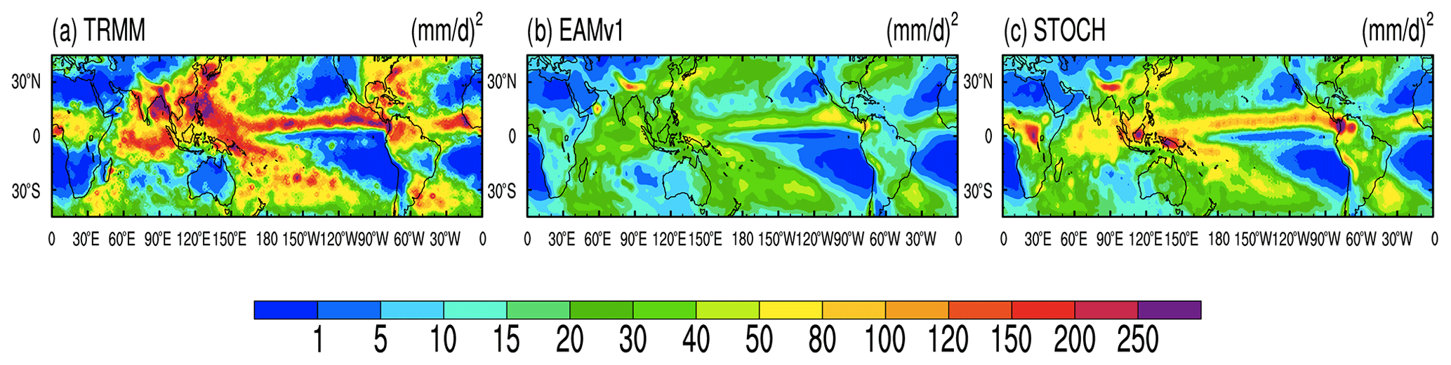
Figure 2 Spatial distributions of the synoptic variance of rainfall from (a) TRMM, (b) EAMv1 and (c) STOCH (units: mm² d⁻²).

Besides the intraseasonal variance, the synoptic variance (2–9 d Lanczos band-pass-filtered rainfall anomalies) is also investigated (Fig. 2). The synoptic-scale variance corresponds to weather activities. In Fig. 2 only TRMM observations are shown to evaluate simulations because the Xie–Arkin observations are pentad data. In TRMM, the geographical distribution of the synoptic variance is similar to that of the intraseasonal variance, but with larger amplitudes because synoptic-scale activities contain much more energy than intraseasonal disturbances. Similar to the intraseasonal variance, the synoptic variance in the EAMv1 run is also much weaker than that in observations. The synoptic-scale variance in the STOCH run is about twice as strong as in EAMv1 although it is still underestimated compared to TRMM observations. Over regions where the overestimated intraseasonal precipitation variance emerges, the STOCH run has excessive synoptic precipitation variance as well. This result is consistent with Goswami et al. (2017), who reported enhanced intraseasonal and synoptic variability of precipitation in the National Centers for Environmental Predictions (NCEP) Climate Forecast System version 2 (CFSv2) using a stochastic multicloud model parameterization.

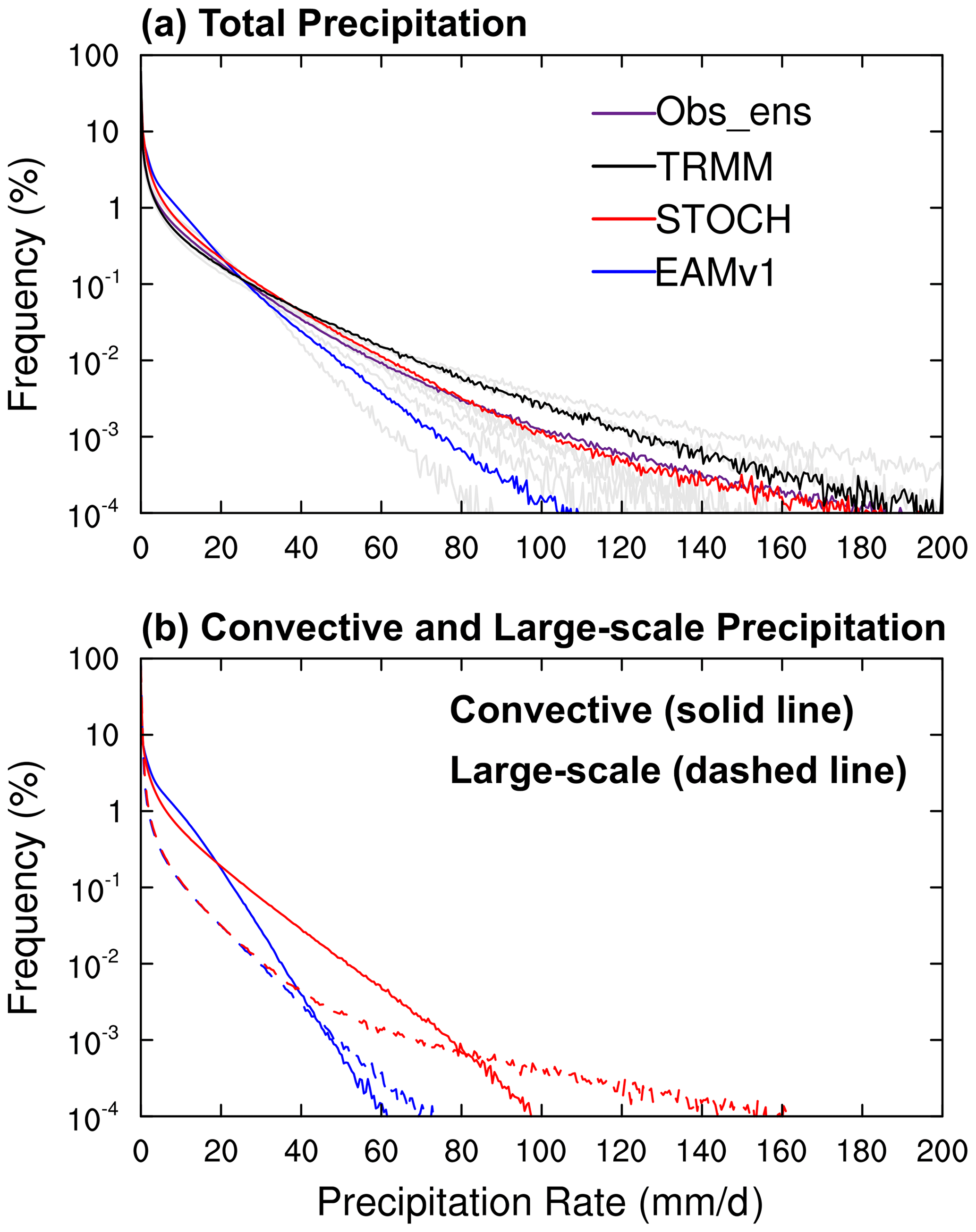
Figure 3 Frequency distributions of (a) total (solid line), (b) convective (solid line) and large-scale (dashed line) precipitation intensity over the tropics (20^∘ S, 20^∘ N) for EAMv1 (blue) and STOCH (red), respectively. For total precipitation, the TRMM observations (black) and the ensemble mean of multiple observations (Obs_ens, purple), with each observation represented by a gray line, are included for evaluation.

3.2 Rainfall frequency, intensity, amount and duration

Wang et al. (2016) showed that the most significant improvement with the use of the stochastic deep convection scheme in CAM5 was in the simulated PDF of rainfall intensity over the tropics, which became very close to TRMM observations. Since there are many modifications in model configuration and physics parameterizations from CAM5 to EAMv1 (Rasch et al., 2019), such as a finer vertical resolution, an updated microphysics parameterization (MG2), and the use of CLUBB in place of separate shallow convection and planetary boundary layer turbulence parameterizations, it is not clear whether a similar degree of improvement in precipitation intensity PDF can be achieved with a similar stochastic convection scheme. Using an equal-interval rainfall intensity bin of 0.5 mm d⁻¹ from 0 to 200 mm d⁻¹, Fig. 3 shows the frequencies of the total precipitation intensity over the tropics (20^∘ S–20^∘ N) from observations, EAMv1 and STOCH. Also shown are the PDFs of large-scale and convective precipitation intensity. The observational uncertainty is larger for intense precipitation than for light precipitation (Fig. 3a), which is consistent with findings in Roca (2019). The GPCP precipitation intensity distribution (the gray curve that even falls below the EAMv1 curve in Fig. 3a) has the lowest frequency for precipitation intensity greater than 30 mm d⁻¹. The GPCP product is known to have underestimated precipitation intensities (Kooperman et al., 2016). Despite the uncertainties in observations, the simulated frequencies in STOCH are more consistent with those in the ensemble mean of all observations than those in the default EAMv1. The stochastic convection parameterization in the STOCH run greatly mitigates the bias of “too much light rain and too little heavy rain”, showing a decrease in the frequency of rainfall intensity between 1 and 10 mm d⁻¹ and an increase in the frequency of rainfall intensity larger than 20 mm d⁻¹ compared to the EAMv1 run. Especially for light rain, the frequencies in STOCH fall in the observational range, while those in EAMv1 do not. A recent study finds that the decreased frequency of light rain has a profound impact on simulated aerosol loading in the atmosphere (Wang et al., 2021a). Xie et al. (2019) indicated that the “too much light rain” in EAMv1 was a result of overly frequent convection. Consistent with this notion, Fig. 3b shows that the reduction of light rain frequency is entirely from convective precipitation. On the other hand, the increase in intense precipitation frequency is from both convective and large-scale precipitation.

To understand why the use of a stochastic convection scheme decreases the frequency of light rain and increases the frequency of heavy rain, we conducted an additional simulation. In the simulation, the setup is identical to the STOCH run except that the ZM scheme is called a second time at each time step, with input (temperature, moisture, etc.) identical to that for the stochastic scheme. However, the output is used for diagnostic purposes only and does not participate in model integration. It is found that (figure not shown) two factors contribute to the decreased frequency of light rain and increased frequency of heavy rain. First, for a given ensemble mean convective mass flux (from the ZM scheme) the probability for cloud generation following the Poisson distribution for a realization in the stochastic scheme can produce more intense precipitation than obtained by the ZM scheme. Second, the probability distribution results in less frequent convection in general. This allows the buildup of atmospheric instability (also see Fig. 9 below in Sect. 3.3), which also leads to heavier convective rainfall (even with the ZM scheme alone without considering the stochastic part) and more large-scale condensation. However, we note that the increase in the frequency of rainfall intensity ranges from 60 to 140 mm d⁻¹ in the STOCH run, which is not as much as that in Wang et al. (2016) for CAM5. This will be elucidated through sensitivity experiments in the next subsection.

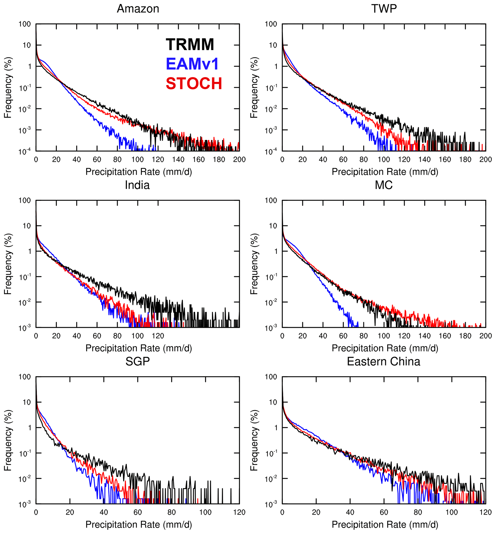
Figure 4 Frequency distributions of total precipitation intensity over the Amazon (20^∘ S–5^∘ N, 40–80^∘ W), the tropical western Pacific (TWP) (0–15^∘ N, 130–170^∘ E), India (14–26.5^∘ N, 74.5–94^∘ E; for June–September), the Maritime Continent (MC) (10^∘ S–10^∘ N, 90–160^∘ E), the Southern Great Plains (SGP) (37–42^∘ N, 90–110^∘ W; for May–August) and eastern China (25–35^∘ N, 100–120^∘ E; for June–August) for TRMM (black), EAMv1 (blue) and STOCH (red).

The frequencies of total precipitation intensity over selected regions also show a qualitatively similar degree of improvement. Figure 4 shows six regions during their convectively active seasons: Amazonia, the tropical western Pacific, and India for June–September; the Maritime Continent and SGP for May–August; and eastern China for June–August in TRMM, EAMv1 and STOCH, respectively. In all tropical regions, the EAMv1 simulation overestimates the occurrence frequency for precipitation intensities less than 20 mm d⁻¹ and underestimates it for precipitation intensities greater than 20 mm d⁻¹, similar to the distribution for the entire tropics. In STOCH, the performance in the PDF over Amazonia and the Maritime Continent is better than the PDF over the entire tropics. Although the biases of “too much light rain” over India and the tropical western Pacific are alleviated by the stochastic deep convection scheme, the bias of “too little heavy rain” remains, particularly over India where large-scale monsoonal dynamics regulate heavy convective rain (Wang et al., 2018). For the two midlatitude convection regions (SGP and eastern China), although there is also noticeable improvement across the precipitation intensity spectrum, it is less significant compared to other regions, possibly because convection in midlatitude land regions is not as prevalent as in the tropics.

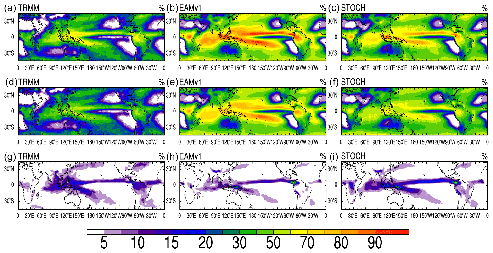
Figure 5 Spatial distributions of the frequencies of total rainfall intensity larger than (a–c) 1 mm d⁻¹, (d–f) between 1 and 20 mm d⁻¹, and (g–i) larger than 20 mm d⁻¹ for TRMM, EAMv1 and STOCH, respectively.

Figure 5 shows the geographical distributions of precipitation frequency for all precipitation, precipitation intensities less than 20 mm d⁻¹ and precipitation intensities more than 20 mm d⁻¹ over the tropics in observations and simulations (days with precipitation intensity less than 1 mm d⁻¹ are considered non-precipitating and thus excluded). In TRMM, the occurrence frequency of rainy days ranges from 30 % to 70 %, with the most frequent rain along the ITCZ, the SPCZ and in the Indian Ocean, where the EAMv1 run has a frequency as high as 80 %–90 %, with up to 30 % positive biases. In contrast, the STOCH run reduces the frequency to 50 %–70 %, although it is still overestimated. When the total precipitation is broken down into precipitation rates less than 20 mm d⁻¹ and precipitation rates above 20 mm d⁻¹, in both observations and simulations the geographical distribution of the rainy days is dominated by days with precipitation intensity less than 20 mm d⁻¹. In comparison with observations, again, the STOCH run reduces the positive bias of the frequency of precipitation intensity less than 20 mm d⁻¹ in the EAMv1 run by up to 20 %. For precipitation intensities greater than 20 mm d⁻¹, the EAMv1 run underestimates their frequency compared to the TRMM observations. On the other hand, the frequency of occurrence in the STOCH run is comparable to the TRMM observations.

Another metric for the precipitation PDF is the contribution of precipitation within a given intensity bin to the total precipitation amount. It combines the information on precipitation frequency distribution and precipitation intensity. While drizzle occurs much more frequently than more intense rain events, it may not contribute much to the total precipitation amount. Following the approach of Kooperman et al. (2016, 2018), we divide the precipitation rate ranging from 0.1 to 1000 mm d⁻¹ into equal bin intervals on a logarithmic scale, with a bin width of $\mathrm{\Delta }\ln \left(R\right)=\mathrm{\Delta }R/R=\mathrm{0.1}$. If the frequency of rainfall rates falling into the ith bin is denoted f_i, then $f_i=n_i/N_{\mathrm{t}}$, where N_t is the total number of days, then n_i is the number of days with rainfall rates falling into the ith bin. The mean precipitation rate in the ith bin is then

$$\begin{array}{}\text{(5)}& R_i={\displaystyle \frac{\mathrm{1}}{n_i}}\sum _{j=\mathrm{1}}^{n_i}{r}_j,\end{array}$$

where r_j is an individual precipitation rate within the ith bin. Thus, the contribution to the total precipitation amount from the ith bin per unit bin width is given by

$$\begin{array}{}\text{(6)}& P_i={\displaystyle \frac{f_i{R}_i}{\mathrm{\Delta }\ln \left(R\right)}}={\displaystyle \frac{\mathrm{1}}{\mathrm{\Delta }\ln \left(R\right)}}{\displaystyle \frac{\mathrm{1}}{N_{\mathrm{t}}}}{\sum }_{j=\mathrm{1}}^{n_i}{r}_j.\end{array}$$

P_i has units of millimeters per day (mm d⁻¹). The total precipitation amount is then given by

$$\begin{array}{}\text{(7)}& P=\sum _i{P}_i\mathrm{\Delta }\ln \left(R\right)=\sum _i{f}_i{R}_i.\end{array}$$

Accordingly, the amount distributions for total (P^T), convective (P^C) and large-scale (P^L) rainfall are given by the following.

$$\begin{array}{}\text{(8)}& {\displaystyle }{P}_i^{\mathrm{T}}={\displaystyle \frac{\mathrm{1}}{\mathrm{\Delta }\ln \left(R\right)}}{\displaystyle \frac{\mathrm{1}}{N_{\mathrm{t}}}}{\sum }_{j=\mathrm{1}}^{n_i}{r}_j^{\mathrm{T}}\text{(9)}& {\displaystyle }{P}_i^{\mathrm{C}}={\displaystyle \frac{\mathrm{1}}{\mathrm{\Delta }\ln \left(R\right)}}{\displaystyle \frac{\mathrm{1}}{N_{\mathrm{t}}}}{\sum }_{j=\mathrm{1}}^{n_i}{r}_j^{\mathrm{C}}\text{(10)}& {\displaystyle }{P}_i^{\mathrm{L}}={\displaystyle \frac{\mathrm{1}}{\mathrm{\Delta }\ln \left(R\right)}}{\displaystyle \frac{\mathrm{1}}{N_{\mathrm{t}}}}{\sum }_{j=\mathrm{1}}^{n_i}{r}_j^{\mathrm{L}}\end{array}$$

Here, r^T, r^C and r^L are the total, convective and large-scale rain rates.

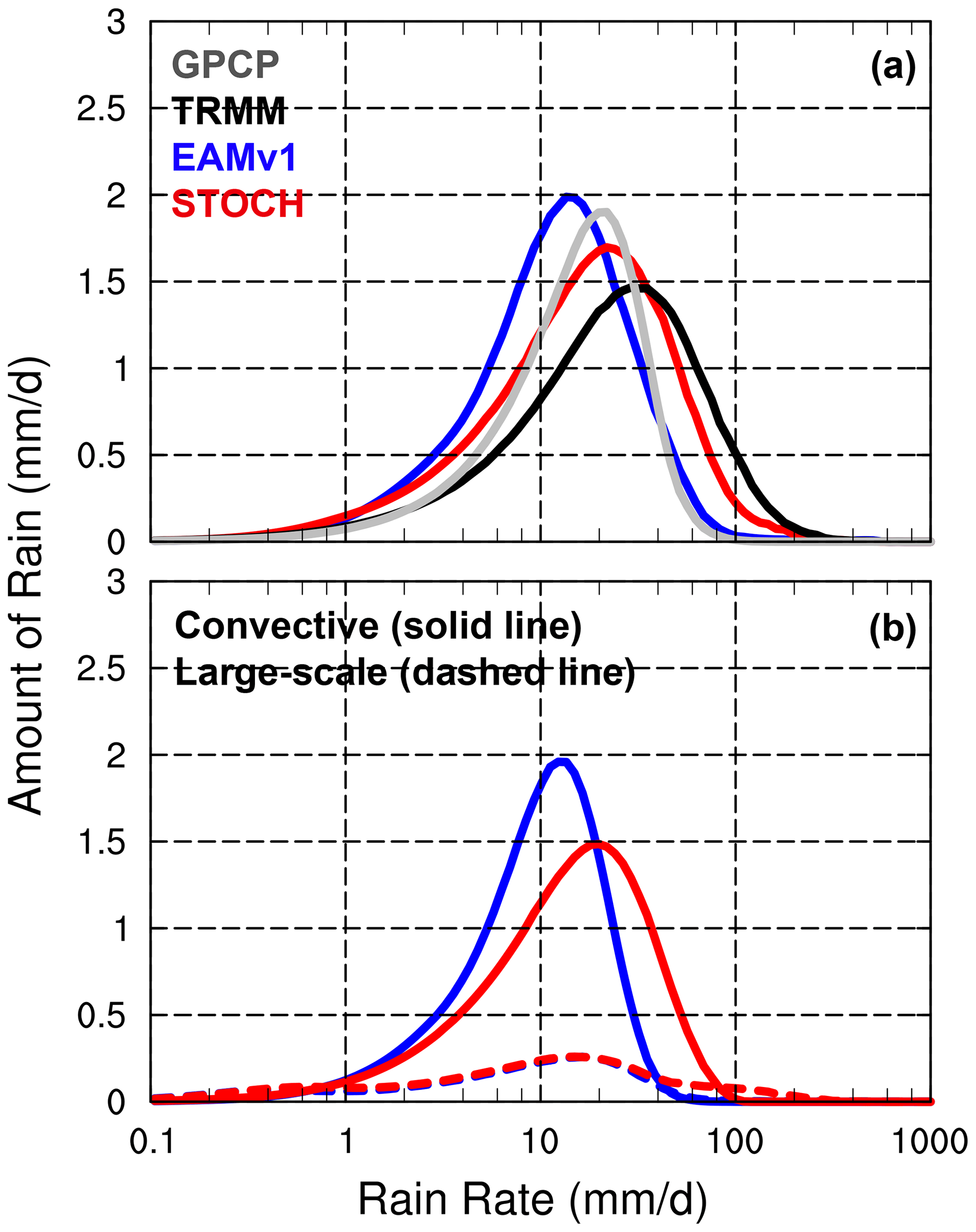
Figure 6 Annual mean rainfall amount distributions of (a) total precipitation (solid line) over the tropics (20^∘ S, 20^∘ N) for GPCP 1DD (gray), TRMM (black), EAMv1 (blue) and STOCH (red). Individual distributions of (b) convective (solid line) and large-scale (dashed line) precipitation in EAMv1 (blue) and STOCH (red) are also shown. The rainfall intensity on the x axis is on a logarithmic scale with bin intervals of $\mathrm{\Delta }\ln \left(R\right)=\mathrm{\Delta }R/R=\mathrm{0.1}$.

Figure 6a shows the contribution to the total rainfall amount from each rainfall rate on a logarithmic scale for GPCP 1DD, TRMM and the two simulations over the tropics. The TRMM observations have larger contributions from intense rainfall rates than GPCP 1DD, with a peak contribution rainfall rate of 28 mm d⁻¹, which is higher than the value of 22 mm d⁻¹ in GPCP 1DD. The EAMv1 run produces a much smaller peak contribution rainfall rate (15 mm d⁻¹) than the two observations, while the STOCH run simulates it realistically (23 mm d⁻¹) as falling between the two observations. Note that precipitation from intensities less than 1 mm d⁻¹ contributes about 0.05 mm d⁻¹ or less to the tropical mean total precipitation, thus justifying treating it as non-precipitating in Fig. 5. Figure 6b shows the convective and large-scale contributions to the simulated total precipitation from EAMv1 and STOCH, respectively. The large-scale precipitation shows very similar contribution distributions in the two simulations except for the largest rain rates, which make only a small contribution to the total. For the most part, large-scale precipitation is not affected by how convection is treated in the model, with both simulations having a maximum contribution near 22 mm d⁻¹. On the other hand, the convective contribution is very different between the two simulations. Similar to the total precipitation, the peak contribution to convective precipitation is at a much smaller rainfall rate in EAMv1 than in STOCH.

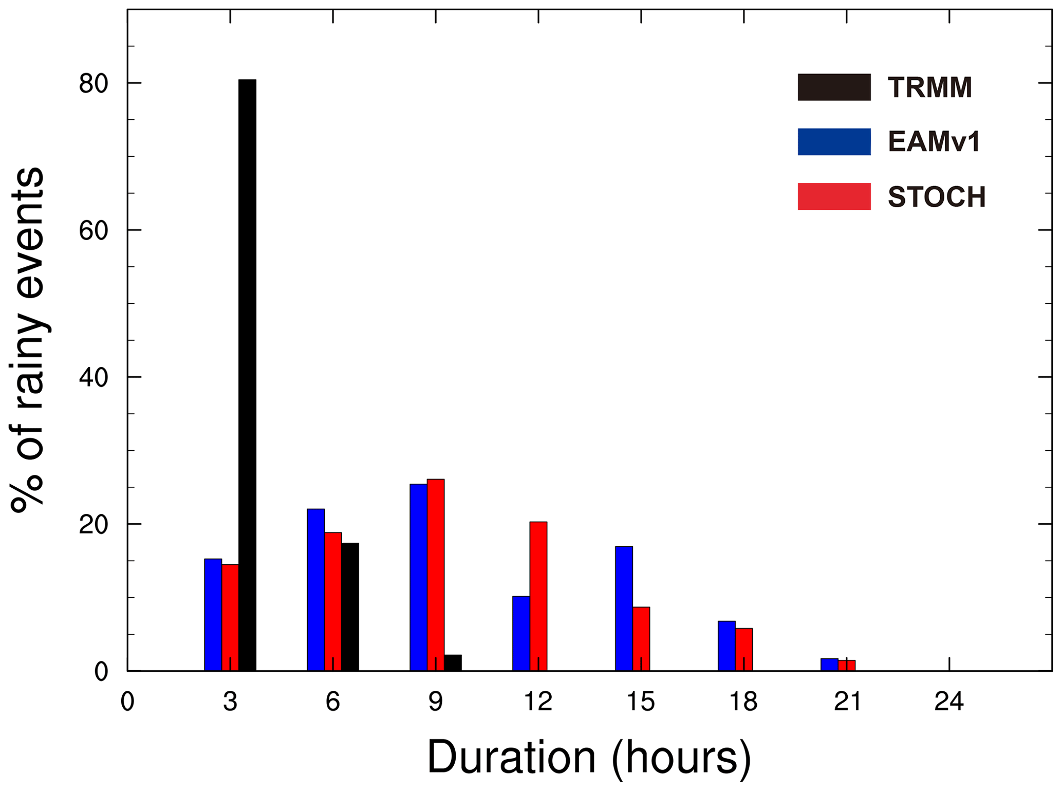
Figure 7 Histogram of the percentage frequency of total rainy events as a function of their duration using 3-hourly data (conditional probability of rainfall given rainfall from previous times) from TRMM (black), EAMv1 (blue) and STOCH (red) for the threshold rainfall rate of 1 mm d⁻¹ over the tropics.

Besides precipitation frequency and intensity, another important higher-order statistic of precipitation is the duration of precipitation events; it measures the intermittency of precipitation (Trenberth et al., 2017). Using 3-hourly data, we calculate the duration of rainfall events as a continuous number of hours of precipitation exceeding a threshold value of 1 mm d⁻¹. Figure 7 shows the frequency of precipitation events for different durations over the tropics; 80 % of TRMM-observed precipitation events last for 3 h or less, 18 % last for 6 h and 2 % last for 9 h. In contrast, both EAMv1 and STOCH produce very small proportions (∼ 15 %) of precipitation events that last for 3 h or less. The frequency of precipitation events lasting 9 h or longer is extremely overestimated in the model simulations, with some lasting for as long as 21 h. This suggests that convection in the model lacks the observed intermittency (Trenberth et al., 2017), and the use of the stochastic convection scheme does not improve this aspect of the simulated convection.

Figure 8 Same as Fig. 3, but including PDFs for EAMv1–30L and STOCH–30L (both dashed lines).

3.3 Sensitivity of rainfall intensity PDF to vertical resolution

A significant modification among several changes in EAMv1 from CAM5 is a much finer vertical resolution, increasing from 30 levels in CAM5 to 72 levels in EAMv1. Within the PBL alone EAMv1 has 17 layers compared to 5 layers in CAM5, and the thickness of approximately 20 m for the lowest model layer in EAMv1 is much thinner than that in CAM5, which is 100 m (Xie et al., 2018). The increased resolution in the PBL in EAMv1 will likely affect the convection behavior through PBL–convection interactions. In Fig. 3 we show that the precipitation intensity PDF is significantly improved with the introduction of the stochastic convection scheme. However, the improvement was not as striking as that shown in Wang et al. (2016) for CAM5. We suspect that this is primarily due to the enhanced vertical resolution in EAMv1 rather than other changes in model physics parameterizations, tunings or the model dynamic core. To confirm this, EAMv1–30L and STOCH–30L runs with a vertical resolution of 30 layers are conducted and compared with the EAMv1 and STOCH runs with the default 72 vertical layers. As seen in Fig. 8, when switching to a configuration of 30 vertical layers, the performance of the STOCH–30L run is very similar to that in CAM5 (Wang et al., 2016). The frequency distribution of rainfall intensity between 60 and 140 mm d⁻¹ almost falls on top of that in TRMM. The PDF of rain intensity in the EAMv1–30L run is also closer to TRMM observations compared to the EAMv1 run (Fig. 8a). For EAMv1, convective and large-scale precipitation becomes more intense in the 30-level configuration. The resolution dependence of large-scale precipitation is consistent with the scale analysis in Rauscher et al. (2016). In their Eq. (2), if the terms are rearranged to solve for vertical velocity (ω), it gives ω∝Δp, the vertical grid spacing in pressure coordinates. Stronger vertical velocity would lead to more intense precipitation. In STOCH–30L, while the frequency of more intense convective precipitation is increased, the frequency of more intense large-scale precipitation is decreased, probably affected by the moisture depletion from strong convective precipitation (Fig. 8b, c).

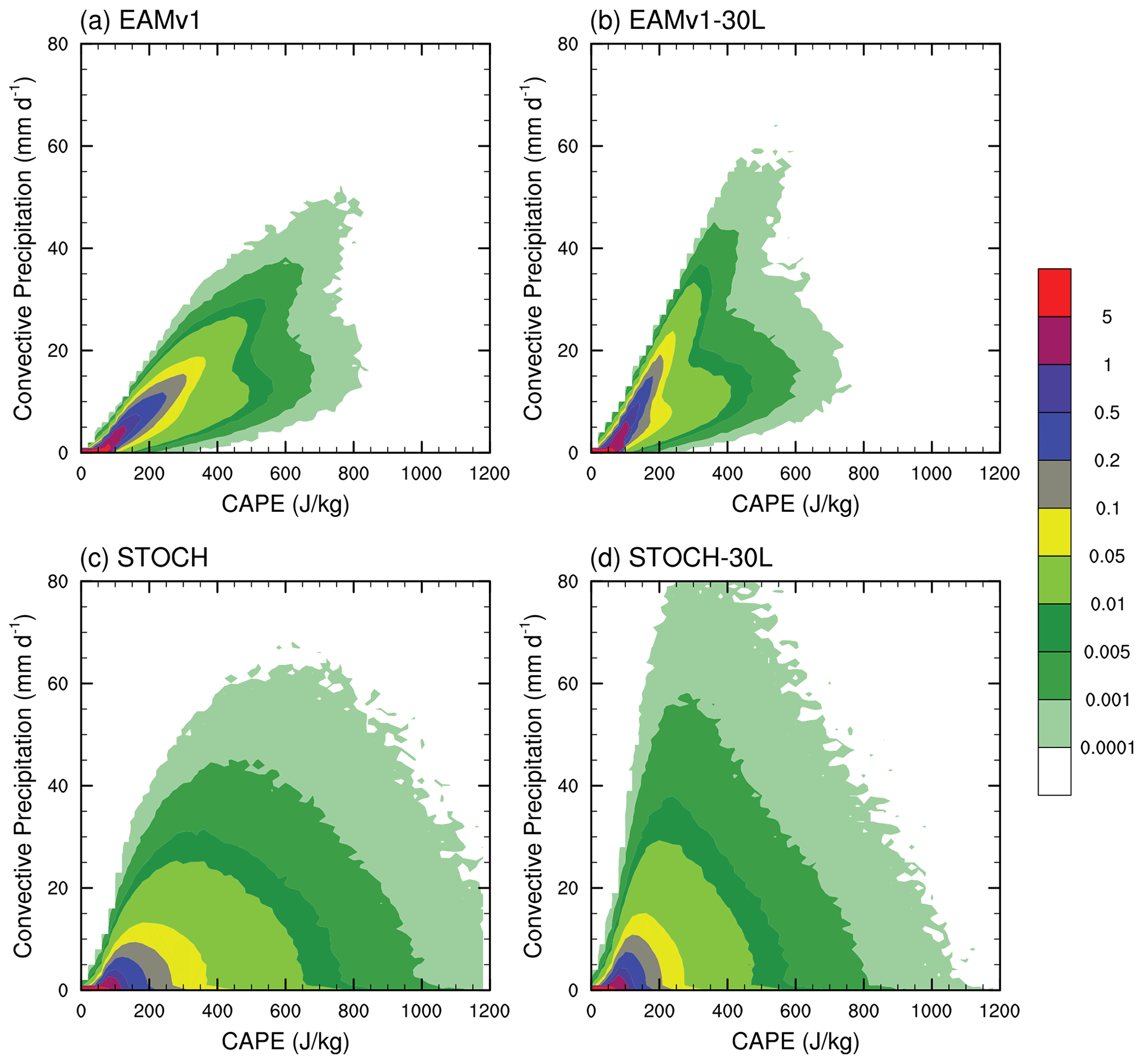
Figure 9 Joint PDFs of CAPE versus convective precipitation over the tropics (20^∘ S, 20^∘ N) from (a) EAMv1, (b) EAMv1–30L, (c) STOCH and (d) STOCH–30L.

The causes of the sensitivity of convective precipitation to vertical resolution are further examined below. In the ZM convection scheme, the amount of convection is linked to dilute CAPE (for convenience we will simply call it CAPE below with the understanding that it refers to dilute CAPE). Thus, in Fig. 9 we present the joint PDF of convective precipitation and CAPE over the tropics in the four simulations. Note that all parameter settings are identical between EAMv1 and EAMv1–30L except the vertical resolution. Both EAMv1 and EAMv1–30L show an approximately linear relationship between CAPE and convective precipitation. The CAPE values are generally smaller in EAMv1–30L than in EAMv1, as can be seen from the frequency of occurrence of both large and medium CAPE values. However, the slope of the maximum occurrence frequency is almost twice as large in EAMv1–30L as in EAMv1 (Fig. 9a, b), giving the higher frequency of larger convective precipitation as seen in Fig. 8. This is because a coarser vertical resolution means stronger vertical mixing, which results in higher precipitation for given CAPE values. For a given precipitation rate that the model produces, there is in general a large range of CAPE values, and the CAPE values in EAMv1 are predominantly larger than in EAMv1–30L as can be seen from the PDF distribution in Fig. 9a and b. Compared to EAMv1, the smaller CAPE values in EAMv1–30L are caused by higher parcel launching levels due to thicker model layers near the surface, where the most unstable air is often found (figure not shown). There is also a bifurcation for medium to large CAPE values. This is likely related to atmospheric moisture conditions in the atmosphere: for the same CAPE values there is less precipitation when the atmosphere is dry and vice versa. With the introduction of the stochastic deep convection scheme, there are no longer approximately linear relations between CAPE and convective precipitation (Fig. 9c, d) in spite of the fact that the CAPE-based closure is still used to determine the cloud-base mass flux (the ensemble mean). This is surprising; it implies that for a given convectively unstable atmospheric thermodynamic condition, the use of the stochastic scheme often inhibits the triggering of convection, thereby allowing for the buildup of CAPE for (the less frequently occurring) stronger convection. Similar to EAMv1, smaller (larger) CAPE values occur more (less) frequently in STOCH–30L due to higher parcel launching levels. Also, the small and moderate values of CAPE have larger probabilities to precipitate more in STOCH–30L compared to STOCH.

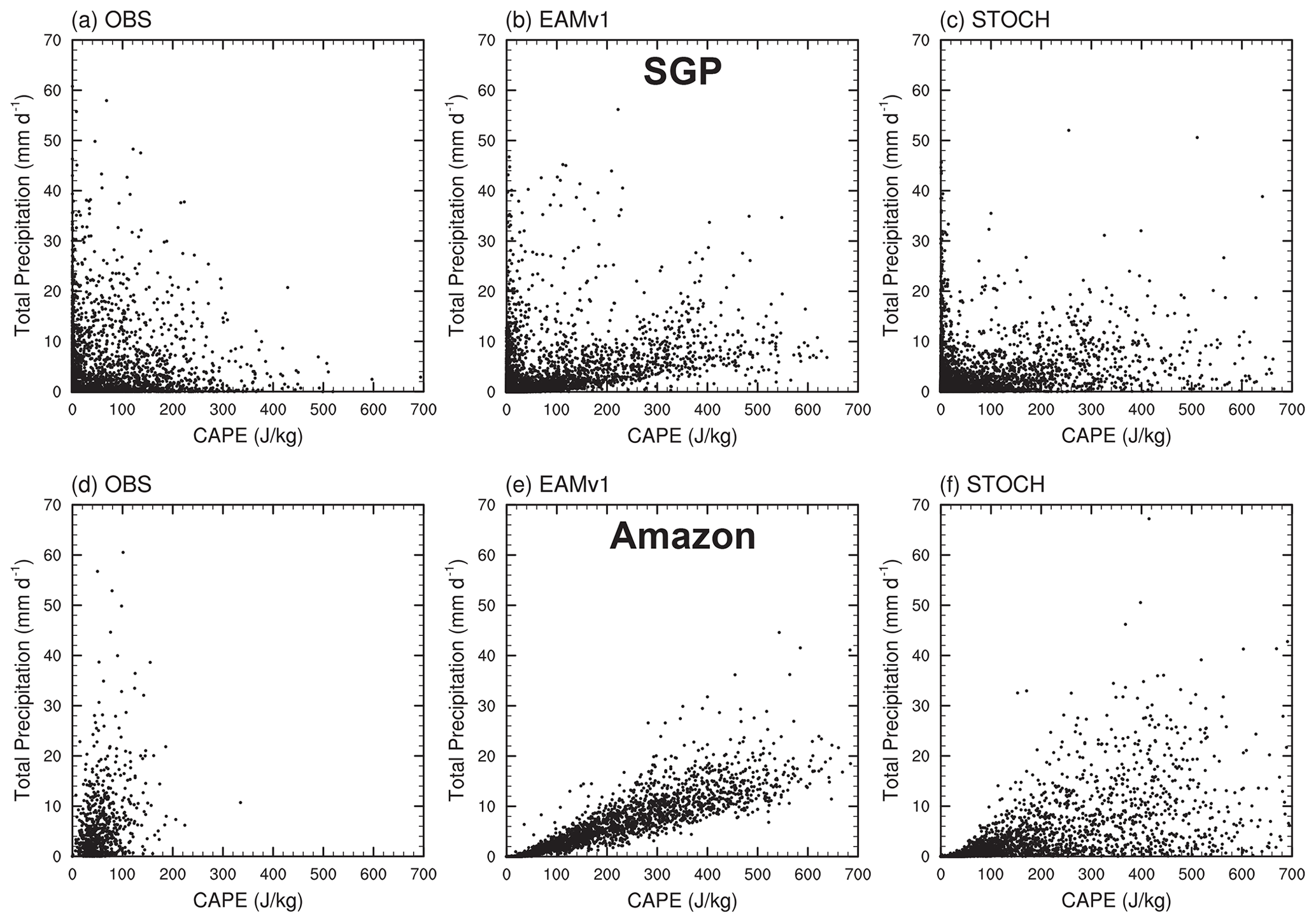
Figure 10 Scatterplots of total precipitation versus CAPE at the ARM (a–c) SGP and (d–f) Amazon sites for (a, d) observations calculated from multiyear sounding data (2014–2015 for the Amazon and 2004–2018 for SGP), (b, e) EAMv1 and (c, f) STOCH.

Over the ARM SGP and GOAmazon sites, no linear relationship is seen between the total precipitation and CAPE in observations (Fig. 10). At the SGP site, high CAPE values generally correspond to low precipitation. At the GOAmazon site, high precipitation values correspond to medium values of CAPE, somewhat resembling the STOCH simulation, although the observed CAPE values at the GOAmazon site are much smaller than those in the simulations.

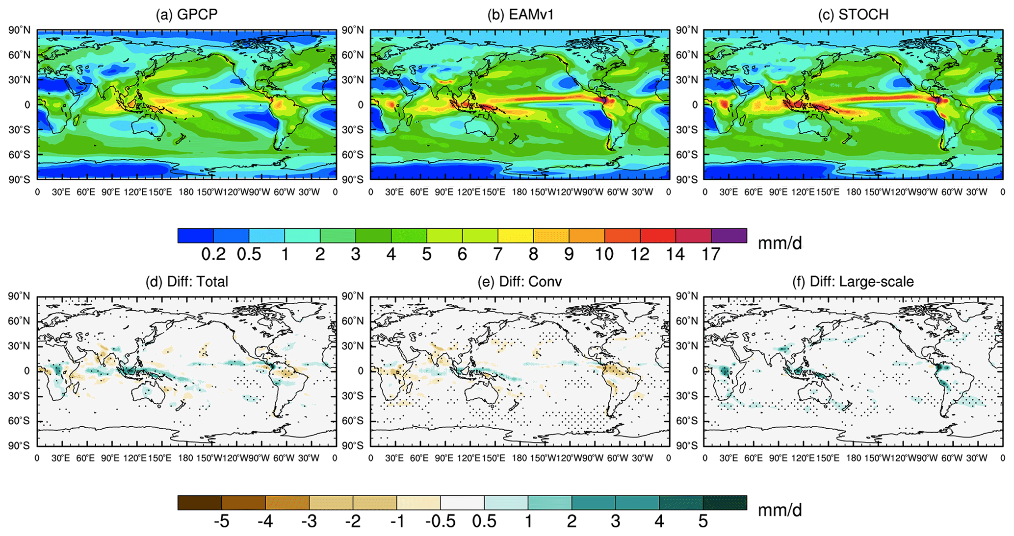
Figure 11 Global distributions of total precipitation for (a) GPCP, (b) EAMv1 and (c) STOCH, as well as the differences of (d) total, (e) convective and (f) large-scale precipitation between STOCH and EAMv1. Differences with a confidence level greater than 95 % in (d–f) are stippled.

3.4 Mean state

So far, we have shown that the introduction of a stochastic convection scheme into the E3SM atmospheric model can significantly improve the simulation of the short-term variability and intensity PDF of precipitation. In climate model development efforts, it is important that an improvement in some aspects of the model does not lead to degradation of other aspects, at least not to outweigh the improvement. Thus, it is imperative that we examine the climate mean fields as well. Figure 11 shows the global distribution of annual mean precipitation in GPCP observations and simulations, as well as the differences in total, convective and large-scale precipitation between the STOCH and EAMv1 runs. Overall, the geographical distributions of precipitation in the two simulations are similar to those in observations, but both overestimate the tropical precipitation (Fig. 11a–c). There is a slight increase in rainfall over the tropical western Pacific, equatorial Indian Ocean and Africa as well as a slight decrease over India and Amazonia in the STOCH simulation (Fig. 11d). Most of these changes are from convective precipitation except over equatorial Africa where the changes are from large-scale precipitation (Fig. 11e, f).

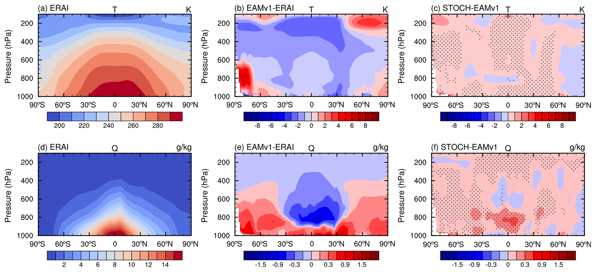
Figure 12 Annual and zonal mean cross sections of (a–c) temperature and (d–f) specific humidity for (a, d) ERAI and differences for (b, e) EAMv1-ERAI and (c, f) STOCH-EAMv1. Differences with a confidence level greater than 95 % between STOCH and EAMv1 are stippled.

The zonal mean of temperature and specific humidity from ERAI and the model biases are shown in Fig. 12. For temperature, EAMv1 produces mostly negative biases in the entire troposphere over the tropics and subtropics and positive biases in the lower troposphere at high latitudes. With the stochastic deep convection scheme used, the temperature changes in STOCH are very minor, increasing slightly from EAMv1. In the simulation of specific humidity, there are positive biases in the lower troposphere across all latitudes and negative biases above 900 hPa over the tropics and subtropics in EAMv1. In comparison with EAMv1, the negative biases are alleviated, but the positive biases are increased slightly in STOCH.

Figure 13 Taylor diagram with metrics for STOCH compared with EAMv1.

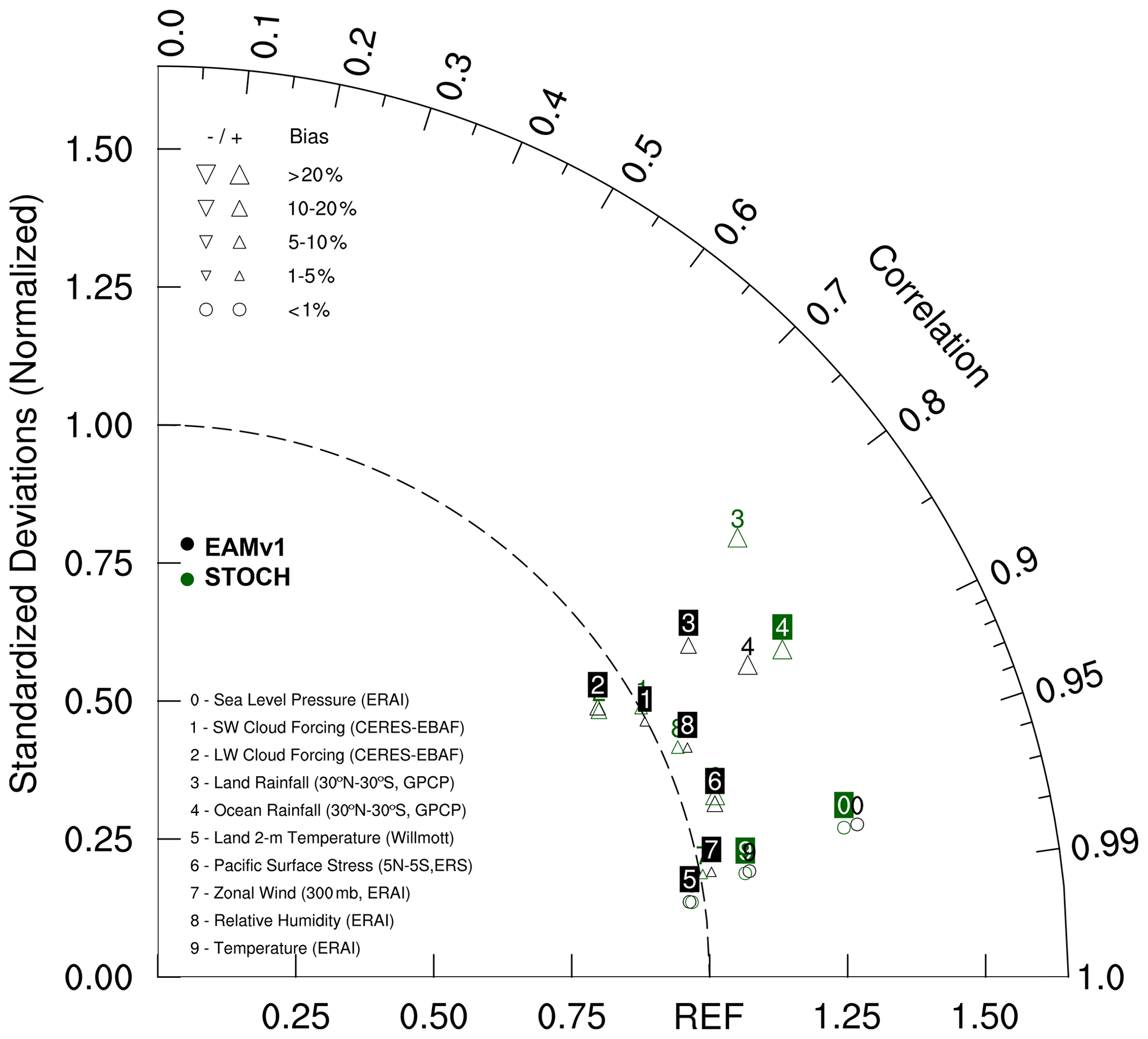
The overall difference in model performance as measured by the commonly used mean climate metrics between EAMv1 and STOCH runs is summarized in a Taylor diagram (Fig. 13). Most metrics are comparable between the two simulations except precipitation, especially over land where STOCH shows a larger standard deviation than both GPCP and EAMv1. In short, the mean climate does not change much after the incorporation of the stochastic convection scheme in EAMv1. This is practically desirable since one does not need to heavily re-tune the model, a task that is often time-consuming and more of engineering than scientific interest.

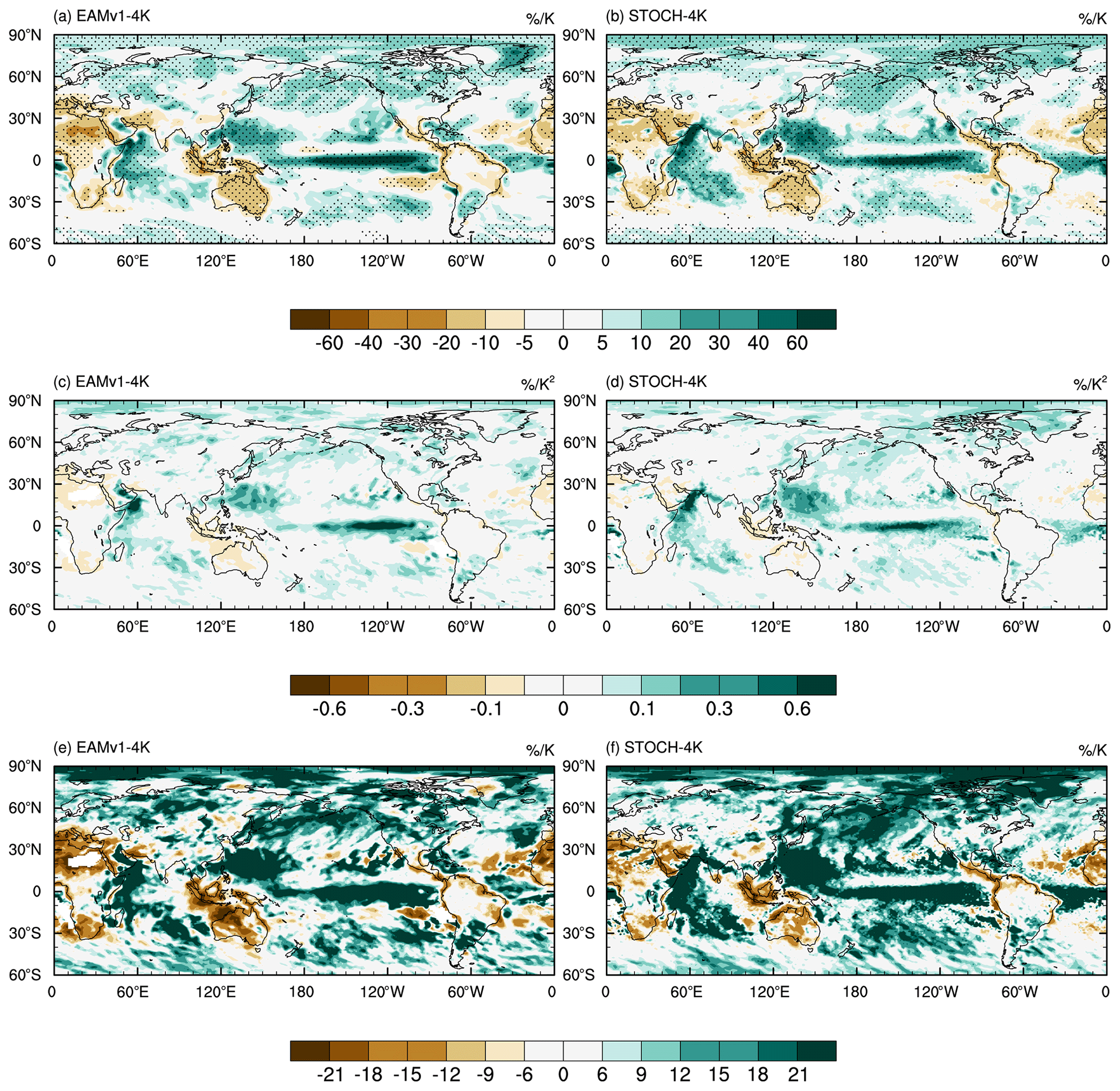
Figure 14 Geographical distributions of the responses of (a, b) annual mean precipitation, (c, d) the coefficient a and (e, f) the fractional change in precipitation extremes (R95p) to climate warming from +4 K experiments. Differences with a confidence level greater than 95 % are stippled.

3.5 Response to climate warming

Another aspect of interest concerns the model's response to climate change. It is well-known that the estimated climate sensitivity for future climate projections is sensitive to changes in model physics parameterizations (Golaz et al., 2019). With the stochastic deep convection parameterization, it is necessary to check if the response of precipitation and associated extremes to climate warming differs. As seen in Fig. 14, relative to the current climate simulations, the geographical patterns and magnitudes of annual mean precipitation changes normalized by the global mean surface air warming (ΔT_sa) in the +4 K SST warming simulations (i.e., $(P_{+\mathrm{4}\mathrm{K}}-P)/P/\mathrm{\Delta }{T}_{\mathrm{sa}}$, units: % K⁻¹) with and without the stochastic deep convection scheme are very similar, with both showing maximum increases over the ITCZ, the western Pacific and the Indian Ocean. Pendergrass et al. (2019) found that the response of extreme precipitation to warming follows a nonlinear relation:

$$\begin{array}{}\text{(11)}& {\displaystyle \frac{\mathrm{d}{r}_x}{\mathrm{d}{T}_{\mathrm{sa}}}}=a{T}_{\mathrm{sa}}\end{array}$$

or

$$\begin{array}{}\text{(12)}& r_x={\displaystyle \frac{\mathrm{1}}{\mathrm{2}}}a{T}_{\mathrm{sa}}^{\mathrm{2}}+b,\end{array}$$

where r_x is a rainfall extreme index (here using R95p, the total rainfall from the days with daily rainfall intensity exceeding 95th percentile of the daily precipitation distribution), T_sa is the global mean surface air temperature in a warmer world, and a is the slope of $\mathrm{d}{r}_x/\mathrm{d}{T}_{\mathrm{sa}}$ versus T_sa measuring the strength of the nonlinear response of extreme rainfall to warming. At each grid point, dr_x≈Δr_x is equal to R95p in a warmer world minus that under the current climate and normalized by the global mean surface air warming (dT_sa≈ΔT_sa). With T_sa in the +4 K SST warming simulations and the calculated $\mathrm{d}{r}_x/\mathrm{d}{T}_{\mathrm{sa}}$, the global distributions of the slope, a (units: % K⁻²), with and without the stochastic deep convection scheme are displayed in Fig. 14c and d. Although the stochastic deep convection parameterization introduces stochasticity into convection and significantly improves the underestimated frequency of intense precipitation under the current climate (Wang et al., 2017), it does not lead to a different nonlinear response of precipitation extremes in a warmer world. The resemblance of the coefficient a between the two simulations results from the similar response of the fractional change in r_x to global warming (Fig. 14e, f). Increasing circulation strength as the climate warms is considered to be the main driver for the nonlinear relationship between tropical precipitation extremes and global mean surface air temperature (Pendergrass et al., 2019), and it is possible that the circulation changes with and without the stochastic deep convection scheme are similar. Relative to their respective current climate states, the responses of the EAMv1–4K and STOCH–4K runs show similar geographical distributions with comparable maximum nonlinearity over the tropical Pacific and Atlantic and the Indian Ocean, which bears some resemblance to that in Pendergrass et al. (2019).

4 Summary

In this study, we implemented the stochastic deep convection scheme (Plant and Craig, 2008; Wang et al., 2016) into the DOE EAMv1 and investigated its impact on the simulation of precipitation. Several improvements are observed with the use of the stochastic convection scheme: (1) the weak intraseasonal and synoptic-scale variabilities in EAMv1 are enhanced to levels much closer to those in observations; (2) the “too much light rain and too little heavy rain” bias over the tropics is significantly alleviated due to less frequent occurrence of drizzling convection and more frequent occurrence of intense large-scale and convective precipitation, contributing to enhanced heavy rain; and (3) the simulated peak precipitation rates (the amount mode) in the precipitation amount distribution, which contribute the most to the total amount of precipitation, are larger and in better agreement with those in TRMM and GPCP observations.

While the improvement in the simulated PDF of rainfall intensity is significant, it is less than what we had expected based on our earlier work with the NCAR CAM5 (Wang et al., 2016). Since there are many changes from CAM5 to EAMv1, including vertical resolution, model dynamic core and physics parameterizations, it is not clear which changes are related to the difference in the improvement of the simulated rainfall PDF. Two sensitivity tests were performed to elucidate this, both with a coarser-vertical-resolution configuration of 30 layers (i.e., EAMv1–30L and STOCH–30L) as in CAM5. The STOCH–30L run successfully reproduces the frequency distribution of rainfall intensity found by Wang et al. (2016), with an increased frequency of convective precipitation intensities between 60 and 140 mm d⁻¹. This increase is explained by the fact that small and moderate values of CAPE generate more convective precipitation from the altered relation between them compared to the 72-level configuration due to fewer model layers in the 30-level resolution. Since vertical velocity in general increases with the vertical grid spacing, the increase in large-scale precipitation also contributes to the increased frequency of total precipitation intensities in the 30-level configuration.

For any changes in model physics parameterizations that improve some aspects of the model performance, it is important that other aspects are not degraded. It is known in the climate modeling community that improved intraseasonal variability is often accompanied by a degradation of the mean state (e.g., Kim et al., 2011; Klingaman and Demott, 2020). We showed that the mean states in tropospheric temperature, moisture and precipitation are not much different with or without the use of the stochastic convection scheme, and neither are the responses of mean precipitation and precipitation extremes to climate warming. This is encouraging and desirable for model development efforts. However, we note that for higher horizontal resolutions (Caldwell et al., 2019) or a regionally refined mesh version of EAMv1 (Tang et al., 2019), spatial averaging of the input fields of the stochastic scheme would be needed to make use of convective quasi-equilibrium over a larger domain. This could be challenging for computational efficiency, and it requires further research in the future.