Using Shapley additive explanations to interpret extreme gradient boosting predictions of grassland degradation in Xilingol, China

Machine learning (ML) and data-driven approaches are increasingly used in many research areas. Extreme gradient boosting (XGBoost) is a tree boosting method that has evolved into a state-of-the-art approach for many ML challenges. However, it has rarely been used in simulations of land use change so far. Xilingol, a typical region for research on serious grassland degradation and its drivers, was selected as a case study to test whether XGBoost can provide alternative insights that conventional land-use models are unable to generate. A set of 20 drivers was analysed using XGBoost, involving four alternative sampling strategies, and SHAP (Shapley additive explanations) to interpret the results of the purely data-driven approach. The results indicated that, with three of the sampling strategies (over-balanced, balanced, and imbalanced), XGBoost achieved similar and robust simulation results. SHAP values were useful for analysing the complex relationship between the different drivers of grassland degradation. Four drivers accounted for 99 % of the grassland degradation dynamics in Xilingol. These four drivers were spatially allocated, and a risk map of further degradation was produced. The limitations of using XGBoost to predict future land-use change are discussed.

1 Introduction

Land-use and land-cover change (LUCC) has received increasing attention in recent years (Aburas et al., 2019; Diouf and Lambin, 2001; Lambin et al., 2003; Verburg et al., 2002). Land-use change includes various land-use processes, such as urbanisation, land degradation, water body shrinkage, and surface mining, and has significant effects on ecosystem services and functions (Sohl and Benjamin, 2012). Grassland is the major land-use type on the Mongolian Plateau; its degradation was first witnessed in the 1960s. About 15 % of the total grassland area was characterised as being degraded in the 1970s, which rose to 50 % in the mid-1980s (Kwon et al., 2016). In general, grassland degradation (GD) refers to any biotic disturbance in which grass struggles to grow or can no longer exist due to physical stress (e.g. overgrazing, trampling) or changes in growing conditions (e.g. climate; Akiyama and Kawamura, 2007). In this study, grassland degradation is defined as grassland that has been destroyed and subsequently classified as some other land use, or that has significantly decreased in coverage.

Grassland is a land use that provides extensive ecosystem services (Bengtsson et al., 2019). When degraded, the consequences are seen in an immediate decline in these services, such as a decrease in carbon storage due to a reduction in vegetation productivity (Li et al., 2017). About 90 % of carbon in grassland ecosystems is stored in the soil (Nkonya et al., 2016). Furthermore, GD results in a reduction in plant diversity and above-ground biomass available for grazing (Wang et al., 2014). Likewise, GD leads to soil erosion and frequent dusts storms in Inner Mongolia (Hoffmann et al., 2008; Reiche, 2014). Drivers of GD are manifold and have been analysed in a range of studies (Li et al., 2012; Liu et al., 2019; Sun et al., 2017; Xie and Sha, 2012). However, few studies use sophisticated driver analysis to predict spatial patterns of GD (Jacquin et al., 2016; Wang et al., 2018). A number of studies have addressed the complex relationship between GD and its drivers (Cao et al., 2013a; Feng et al., 2011; Fu et al., 2018; Tiscornia et al., 2019a). However, these studies focus mainly on visualising or describing non-linear relationships between GD and its drivers.

The aim of developing various land-use models was to explore the causes and outcomes of land-use dynamics; these models were implemented in combination with scenario analysis to support land management and decision-making (National Research Council, 2014; Ren et al., 2019). Most such models are statistical models, such as logistic regression models or models based on principle component analysis (Li et al., 2013; Lin et al., 2014) or Bayesian belief networks (Krüger and Lakes, 2015). Some such models are spatially explicit (e.g. CLUE-S, GeoSOS-FLUS, LTM, Fu et al., 2018; Liang et al., 2018a; Pijanowski et al., 2002, 2005; Verburg and Veldkamp, 2004; Zhang et al., 2013); others are not (e.g. Markov models; Iacono et al., 2015; Yuan et al., 2015). Hybrid models, which combine different approaches to make the best use of the advantages of each model, are another important variety. This type of model is used to characterise the multiple aspects of LUCC patterns and processes (Li and Yeh, 2002; Sun and Müller, 2013). Agent-based models (ABM) simulate land use change decisions based on the behaviour of individual decision-makers. They often consider economic and political information to calculate land-use change. Cellular automata (CA) models are gridded models in which time, space, and state are all discrete. CA models are spatially explicit and land use change decisions are made based on the state of the neighbouring cells (Yang et al., 2014). CA models are often used for the spatial allocation of land use and land cover at a high spatial resolution (Cao et al., 2019) and may be used in combination with other models, such as ABM (e.g. Charif et al., 2017; Mustafa et al., 2017; Troost et al., 2015; Vermeiren et al., 2016).

In most cases of land-use change, it was either assumed that the relationship between the drivers and the resulting land-use change is constant over time (Fu et al., 2018; Samie et al., 2017; Zhan et al., 2007), or the relationships were identified as being linear or non-linear but were not interpreted (Tayyebi and Pijanowski, 2014a). We hypothesise that the relationships between GD and its drivers are mainly non-linear. We therefore see a need for methods that are capable of analysing and interpreting non-linear relationships between GD and dynamic drivers.

With the development of computer science, machine learning (ML) models have been increasingly used in land-use change modelling (Islam et al., 2018; Krüger and Lakes, 2015; Lakes et al., 2009; Tayyebi and Pijanowski, 2014a). ML is superior to the human brain when it comes to pattern recognition in large datasets, e.g. images and sensor fields. Once the task is defined and the data for training are provided, ML operates without any further human assistance. Various ML approaches have been used in the analysis of land-use change processes, the most prominent of which are support vector machines (SVM; Huang et al., 2009, 2010), artificial neural networks (ANN; Ahmadlou et al., 2016; Yang et al., 2016), classification and regression trees (Tayyebi and Pijanowski, 2014b), and random forest (RF; Freeman et al., 2016). While the different ML approaches generally perform well in identifying patterns, they remain a black box and make no contribution to our understanding of how the underlying drivers act on the LUCC process. Compared to linear methods such as logistic regression, ML models often achieve higher accuracy and capture non-linear land-use change processes. Likewise, ML models relax some of the rigorous assumptions inherent in conventional models, but at the expense of an unknown contribution of parameters to the outcomes (Lakes et al., 2009). However, the key challenge is to crack the black box and reveal how each driver affects the land-use change pattern or processes in the ML models.

The extreme gradient boosting (XGBoost) method has recently been developed as a supervised machine learning approach (Chen and Guestrin, 2016). XGBoost algorithms have achieved superior results in many ML challenges; they are characterised by being 10 times faster than popular existing solutions, and the ability to handle sparse datasets and to process hundreds of millions of examples. XGBoost has already been used in land-use change detection, combined with remote sensing data (Georganos et al., 2018), but has not yet been used in the simulation and prediction of land-use change. Shapley additive explanations (SHAP; Lundberg and Lee, 2017) is a unified approach to explain the output of any ML model and to visualise and describe the complex causal relationship between driving forces and the prediction target. We propose using SHAP to analyse the driver relationships hidden in the black box model of XGBoost when employed for land-use change modelling.

Having earlier used a clustering approach to identify drivers of GD in a case study in Inner Mongolia (Xilingol League; Batunacun et al., 2019), we now use XGBoost and SHAP to simulate GD dynamics across the same area. We are primarily interested in learning whether ML models can achieve a better predictive quality than linear methods, in addition to improving our understanding of how grassland degrades in Xilingol. With the intention to identify areas with a high risk of further degradation and to determine the drivers responsible for progressive degradation, we used XGBoost to generate a data-driven model to explore the GD patterns. We then used SHAP to open the non-linear relationships of the black box model stepwise and transformed these relationships into interpretable rules. The resulting model enabled us to map the primary GD drivers and GD hot spots in Xilingol.

2 Materials and methods

2.1 Study area

The Xilingol League is located about 600 km north of Beijing (He et al., 2004), in the centre of Inner Mongolia. This administrative unit, covering an area of 206 000 km², spans from 41.4 to 46.6^∘ N and from 111.1 to 119.7^∘ E (Fig. 1). The area is dominated by the continental temperate semiarid climate. The frequent droughts (in summer) and “dzud” (an extremely harsh and snow-rich winter) are the major natural disasters that occasionally lead to catastrophic livestock losses in this region (Allington et al., 2018; Tong et al., 2017; Xu et al., 2014). Xilingol possessed about 18 104 km² available pasture resources and 1240.4×10⁴ sheep units at the end of 2015 (Xie and Sha, 2012). Around 1.044 million people lived in Xilingol in 2015, with ethnic Mongolian minorities accounting for around 31 % and the rural population for 37 % (Batunacun et al., 2019; Shao et al., 2017). Xilingol is a vast grassland, known for its high-quality meat products, nomadic culture, rich mineral resources, and ethnic minorities. The ongoing degradation of grassland is receiving increasing attention. A set of economic stimuli and ecological protection policies launched in Xilingol were viewed as the root cause of GD over the past four decades. Although large-scale ecological restoration policies were implemented after 2000 in a bid to reduce GD, the problem still persists.

Figure 1 The location of the Xilingol League in Inner Mongolia and its land uses.

2.2 Grassland degradation

This study defines grassland degradation based on land-use conversion, involving two kinds of land-use change processes: (i) the complete destruction of grassland by transformation to another type of land use (built-up land, cropland, woodland, water bodies, and unused land), and (ii) a decline in grassland coverage, which includes dense grass deteriorating into moderately dense grass and sparse grass, and moderately dense grass deteriorating into sparse grass (see Fig. S1a in the Supplement). Given that GD is a dynamic process, we intended in this study to find the major drivers of newly added grassland degradation (NGD). NGD refers to the difference in spatial GD extent between two periods. About 13.0 % of the total grassland area (176 410 km² in 2015) was degraded between 1975 and 2000 (Fig. S1b); a further 10.6 % was degraded in 2000–2015 (Fig. S1c). Comparing the two periods, approximately 10.2 % of the grassland corresponded to the NGD area across the whole region (Fig. S1d). In total 18 279 pixels were extracted from the total NGD area, while the pixel number of conversion for other land uses is 181 190 in this study (hereafter: non-NGD).

2.3 Data collection

In line with previous studies, a checklist of possible drivers (D) of GD was developed from the literature (Cao et al., 2013b; Sun et al., 2017). A total of 19 drivers were grouped into four categories (see Table 1). All categories were described as follows: (1) Climate factors, including the annual mean temperature (T) and annual sum of precipitation (P) in the growing season (April to September), were extracted from the longest available weather dataset (from 1958–2015), in combination with evaluation data and the kriging algorithm, to produce 1×1 km² raster files. (2) Geographic factors include elevation (DEM), and slope and aspect (extracted from DEM data), which can be treated as the characteristic of each grid cell. The DEM data were extracted from the SRTM 90 m resolution and, after resampling using the NEAREST method in ArcGIS, all data were processed into 1×1 km² raster files. (3) Distance measures (the distance of each pixel centre to urban, rural, road and mining, forest, cropland, dense grass, moderately dense grass, sparse grass, and unused land pixels) are widely used factors for different land-use models (Khoury, 2012; Samardžić-Petrović et al., 2016, 2017; Zhang et al., 2013). All distance measures were extracted from LUCC datasets from the years 2000 and 2015 using ArcGIS Euclidean distance and processed into 1×1 km² grids. (4) Socio-economic factors include the gross domestic product (GDP) and population density from 2000 and 2010, and sheep density from 2000 and 2015. GDP and population density were obtained from a resources and environment data cloud platform, CAS (http://www.resdc.cn/, last access: 8 February 2020); sheep density data were accessed from statistical data, and we converted all livestock data into grassland pixels. Unfortunately, high-resolution GDP and population density data were not available for 2015 to match the other data that were recorded for that year, so we may assume that GDP and population density introduce a bias to the result. While population density did not change much between 2010 and 2015, GDP changed from CNY 61.4 billion in 2010 to CNY 100.2 billion in 2015 in total over the Xilingol region (GDP data source: http://tjj.xlgl.gov.cn/ywlm/tjsj/jdsj/, last access: 1 April 2020). (5) Finally, we identified an area in which we assumed a strong policy impact in the past and developed a proxy for the policy effect on grassland degradation. Here, a range of ecological protection measures were implemented inside and outside the Hunshandake and Wuzhumuqin sand lands (see Fig. S2), e.g. a livestock ban and the promotion of chicken farming (Su et al., 2015). In a bid to explore policy effects, we assumed that GD is effectively slowed down by various policies inside the sandy area (proxy set as 0), while outside the sandy area, land degradation is more likely to happen in the absence of any policy effect (proxy set as 1; see Fig. S2).

Table 1 Definition and derivation of drivers.

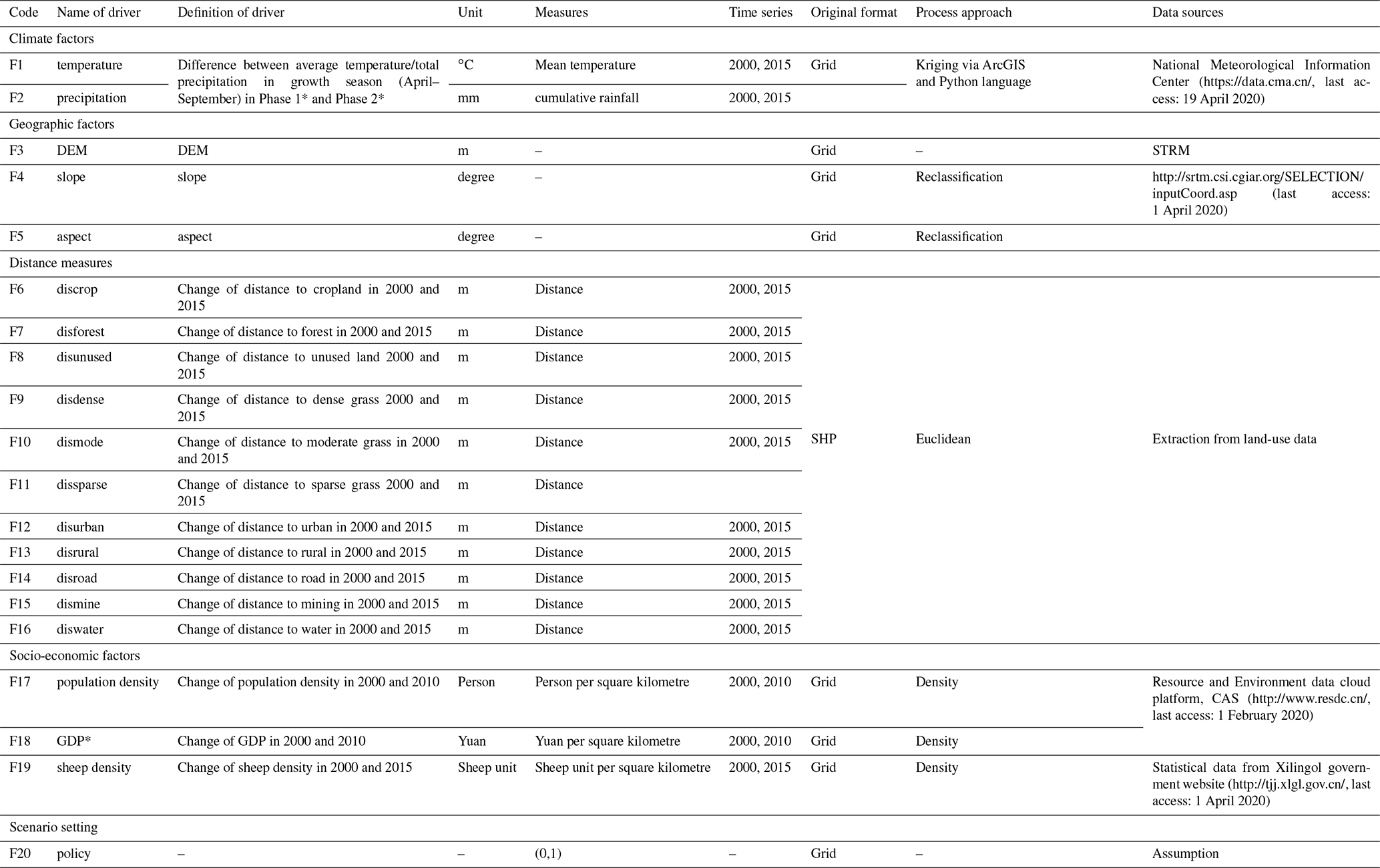
* Note: Phase 1 refers to 1975–2000, and Phase 2 refers to 2000–2015. GDP: gross domestic product.

2.3.1 XGBoost and logistic regression

Two algorithms were selected in this study: logistic regression (LR) and XGBoost. LR is a linear method involving two parts: the statistic LR and the classification LR. Both methods have already been used to simulate land use (Lin et al., 2011; Mustafa et al., 2018) and to define the relationship between land-use change and its drivers (Gollnow and Lakes, 2014; Mondal et al., 2014; Verburg et al., 2002; Verburg and Chen, 2000). Here, we use LR as a benchmark model to compare linear and non-linear methods in the simulation of land-use change. The optimised parameters of LG are C=0.1, penalty = l2, solver = “lbfgs”, and multi_class = “multinomial”.

Boosting algorithms have been implemented in many past studies, where they often outperformed other ML algorithms (Ahmadlou et al., 2016; Filippi et al., 2014; Freeman et al., 2016; Keshtkar et al., 2017; Tayyebi and Pijanowski, 2014a). However, traditional boosting algorithms are often subject to overfitting (Georganos et al., 2018). To overcome this problem, Chen and Guestrin (2016) presented a new, regularised implementation of gradient boosting algorithms, which they called XGBoost (extreme gradient boosting). XGBoost was built as an enhanced version of the gradient boosting decision tree algorithm (GBDT), a regression and classification technique developed to predict results based on many weak prediction models – the decision tree (DT) (Abdullah et al., 2019; Freeman et al., 2016). XGBoost provides strong regularisation by adopting a stepwise shrinkage process instead of the traditional weighting process provided by GBDT. This process limits overfitting, minimises training losses and reduces classification errors while developing the final model (Abdullah et al., 2019; Hao Dong et al., 2018).

The XGBClassifier uses the following parameters: learning_rate (controls learning itself); max_depth (control depth of the RF); the n_estimators (controls the number of estimators used for the model); the min_child_weight (controls the complexity of a model, defines the minimum sum of weights of all observations required in a child); and lambda (L2 regularisation term on weights). The parameters were optimised using a simple grid search algorithm provided by scikit (Pedregosa et al., 2011) to estimate the optimal parameters (learning_rate = 0.1, max_depth = 9, n_estimater = 500, min_child_weight = 3, lambda = 10).

2.3.2 Sampling methods

Data are often distributed unevenly among different classes (Vluymans, 2019). Such imbalanced class distribution generally induces a bias. Canonical ML algorithms assume that data are roughly balanced in different classes. In real situations, however, the data are usually skewed, and smaller classes often carry more important information and knowledge than larger ones (Krawczyk, 2016). It is therefore important to develop learning from imbalanced data to build real-world models (Krawczyk, 2016; Vluymans, 2019). To ensure a highly accurate GD model, we introduced four different sampling methods in this study (Fig. S3).

Balanced sampling. This consists of random data sampling, resulting in equal-sized samples.

Imbalanced sampling. This consists of random data sampling, but with the same share of the sampled class, resulting in unequal sized samples.

Over-sampling. Artificial points are added to the minority class of an imbalanced sampling set, making it equal to the majority class and resulting in equal sized samples.

Under-sampling. Points are removed from a majority class of an imbalanced sampling set, making it equal to the minority class and resulting in equal sized samples (He and Garcia, 2009).

In the present study, we used these four sampling methods to evaluate the model in the context of the sampling method and its performance in the training process and the simulation process (see Fig. S3). In our case study, 20 000 pixels (about 10 % of the total; including 18 190 pixels with value 0 indicating no-change areas and restored grassland and 1810 pixels with value 1 indicating newly added grassland degradation) were selected by different sampling methods (Fig. S3) to train (66 % of the sample size) and test (34 % of the sample size) the model.

2.3.3 SHAP values

SHAP (Shapley additive explanations) is a novel approach to improve our understanding of the complexity of predictive model results and to explore relationships between individual variables for the predicted case (Lundberg and Lee, 2017). SHAP is a useful method to sort the driver's effects and break down the prediction into individual feature impacts. Feature selection is of primary concern when using ML methods to process land-use change (Samardžić-Petrović et al., 2015, 2016, 2017). SHAP values show the extent to which a given feature has changed the prediction and allows the model builder to decompose any prediction into the sum of the effects of each feature value and explain – in our case – the predicted NGD probability for each pixel (see Fig. 2). In this study, we used SHAP values to sort the driver's attributions, capture the relationship between drivers and NGD, and map the primary driver for NGD at the pixel level.

Figure 2 Decomposed SHAP values for the individual prediction of an example pixel.

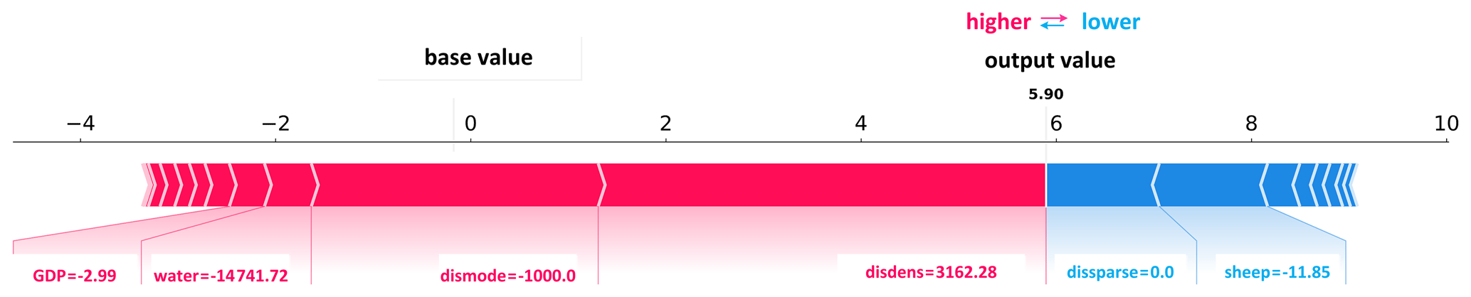
In our study, we define the base value as the value that would be predicted by the model if no feature knowledge were provided for the current output (mean prediction); we define the output value as the prediction for this particular observation. SHAP values are calculated in log odds. Features that increase the value of the prediction (to the left in Fig. 2) are always shown in red; those that lower the prediction value are shown in blue (to the right in Fig. 2, Dataman, 2019). In this instance (Fig. 2), disdense (change of distance to dense grass) is the primary driver of NGD at this pixel level (largest value). The fact that the value is positive means that the risk of NDG increases in line with an increase in distance to dense grass areas.

2.3.4 Validation of the model

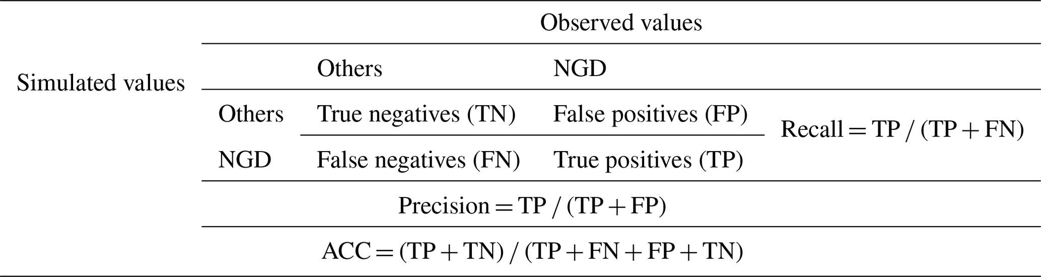
Two validation steps are required for ML models: validation of the training process and validation of the simulation process. For the training process, a robust model was selected using overall classification accuracy, precision, recall, and the kappa index. Accuracy, precision, and recall were calculated based on a confusion matrix (CM) (see Table 2) (He and Garcia, 2009). For the simulation process, the final model was validated using the kappa index, the area under the precision–recall (PR) curve, and recall. The validation indicators are defined as follows.

Overall classification accuracy (ACC) is the correct prediction of NGD and other pixels in the whole region. This indicator was used to evaluate the accuracy of the model. Precision is the proportion of correctly predicted positive examples (which refers to NGD in this study) in all predicted positive examples. Recall is the proportion of correctly predicted positive examples in all observed positive examples (the observed NGD) (Sokolova and Lapalme, 2009). In general, high-precision predictions have a low recall, and vice versa, depending on the predicted goals. Here, since we focus on NGD and other land-use changes, we use both indicators to evaluate our models.

Table 2 Confusion matrix for binary classification of newly added grassland degradation (NGD) and other changes, including four indicators: false positives (FP), cells that were predicted as non-change but changed in the observed map; false negatives (FN), cells that were predicted as change but did not change in the observed map for disagreement; true positives (TP), cells that were predicted as change and changed in the observed map; and true negatives (TN), cells that were predicted as non-change and did not change in the observed map for agreement.

The precision–recall curve provides more information about the model's performance than, for instance, the receiver operator characteristic curve (ROC curve), when applied to skewed data (Davis and Goadrich, 2006). The PR curve shows the trade-off of precision and recall and provides a model-wide evaluation. The area under the PR curve (AUC-PR) is likewise effective in the classification of model comparisons. The baseline for the PR curve (y) is determined by positives (P) and negatives (N). In our study, y=0.09 (y=18 374/200 652), which means when AUC-PR = 0.09, the model is a random model (Brownlee, 2018; Davis and Goadrich, 2006).

The kappa index (κ) is a popular indicator used to measure the proportion of agreement between observed and simulated data, especially to measure the degree of spatial matching. When κ>0.8, strong agreement is yielded between the simulation and the observed map, $\mathrm{0.6}<\mathit{\kappa }<\mathrm{0.8}$ describes high agreement, $\mathrm{0.4}<\mathit{\kappa }<\mathrm{0.6}$ describes moderate agreement, and κ<0.4 represents poor agreement (Landis and Koch, 1977).

In this study, κ was used to evaluate the agreement and disagreement between observed NGD and simulated NGD. Kappa should be the primary validation measure, followed by AUC-PR (used to evaluate model performance) and recall (used to evaluate model sensitivity). Features and definitions of these indicators are given below.

2.3.5 The structure of the ML model

The ML methodology of simulating GD involves six steps (Fig. S4).

1. Target definition and data collection and processing. The targets of this study are to build a robust ML model for simulating NGD, as well as visualising these complex relationships between various variables and the dynamics of GD. A total of 20 drivers of GD were collected. All dynamic drivers were processed by GIS into raster files and exported into ASCII files as final inputs for the ML model.

2. Data organisation. The ML model simulates land-use change as a classification task (Samardžić-Petrović et al., 2015, 2017). In the present study, we organise this task as a binary classification Y (value 1 and 0, stand for NGD and Non-NGD); related drivers are x ($x_{\mathrm{1}},x_{\mathrm{2}},x_{\mathrm{3}}\mathrm{\dots }\mathrm{\dots }{x}_n$), n is the driver identifier, and x denotes the change in value of each driver. The process of data standardisation is usually necessary for most ML models, but since XGBoost is a tree-based method, it does not require standardisation or normalisation. In this case, we performed standardisation only for the logistic regression model.

3. Data sampling. This is a necessary step to avoid overfitting or the loss of important information. The sampling method generally includes balanced and imbalanced sample strategies. In this study, we tested various balanced sampling strategies to identify the most suitable one.

4. Model building and selection. A ranking was used to find the best model in each specific case. In our study, we defined a model with κ>0.8 and AUC-PR >0.09 as robust, while $\mathrm{0.6}<\mathit{\kappa }<\mathrm{0.8}$ and AUC-PR >0.09 represents an acceptable model.

5. Model validation and feature ranking. After tuning the model, the most robust model and the driver with most useful information are selected.

6. Explanation. The last step is explaining the model and the simulation. The model used in the training process was published in Zenodo (Batunacun and Wieland, 2020).

3 Results

3.1 Model validation

The XGBoost model outperformed the LG model in both training and simulation (Figs. 3 and 4). The LG model seems to be an inappropriate model for understanding NGD in this case. XGBoost yielded robust results in both training and simulation, with indicator values almost entirely above 90 %.

Figure 3 indicates that XGBoost performed very well across all balanced sampling methods (over-sampling, under-sampling, and balanced sampling; red rectangle in Fig. 3) in the training process. Only the imbalanced sampling exhibited a slightly weaker performance in the training process. This is mainly due to the balanced sampling datasets, which provided more information for the model. In addition, the model was affected less than the imbalanced sampling method by the majority class or unchanged cells (Samardzic-Petrovic et al., 2018).

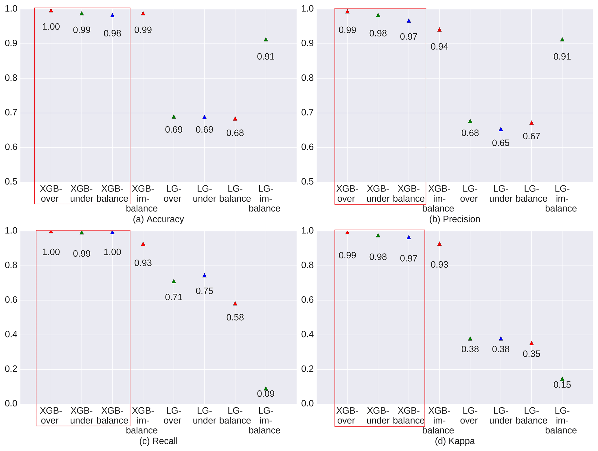
Figure 3 Evaluation of model performance during the training process for newly added grassland between 1975–2015.

Figures 4 and 5 show the model evaluation results in the simulation process and the spatial prediction maps. XGBoost with under-sampling (green rectangle in Fig. 4) yielded the weakest performance compared to the other three sampling methods. This is mainly due to the smaller sample size, which prevents the model from extracting sufficient experience. As can be seen in Fig. 5b, XGBoost used with the under-sampling method produced the error map with the highest FP values, where the model predicted non-change points as change points. The under-sampling method is unable to identify NGD points sufficiently well. XGBoost used with the over-sampling method caused balanced and imbalanced sampling to have similar and strong prediction abilities (see Fig. 4), differing only slightly in their CM indicators (see Fig. 5). We finally selected XGBoost combined with the over-sampling strategy for our study, mainly because of its relatively higher values in κ, AUC-PR, and recall (see Fig. 4).

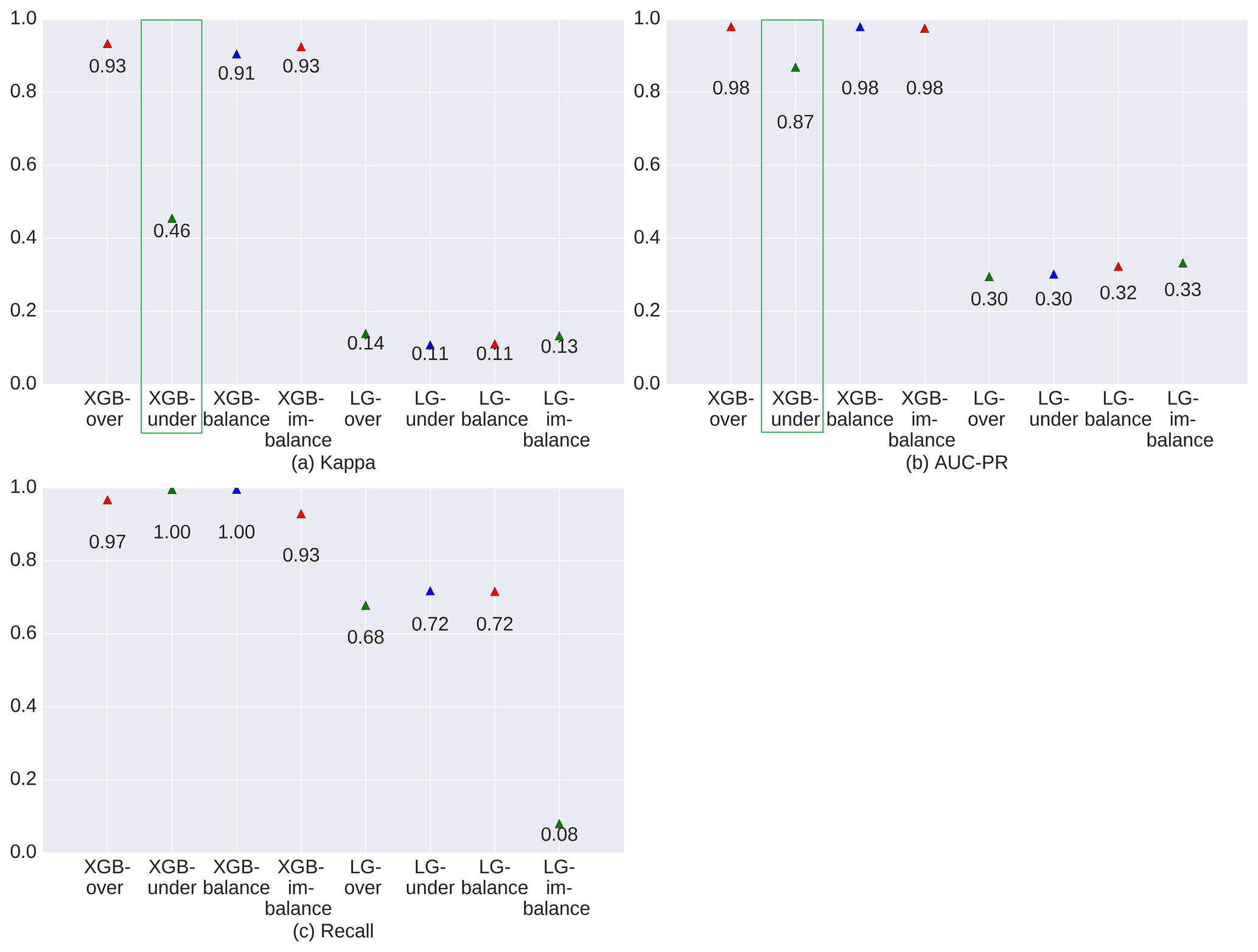
Figure 4 Evaluation of model performance during the prediction process for newly added grassland between 1975–2015.

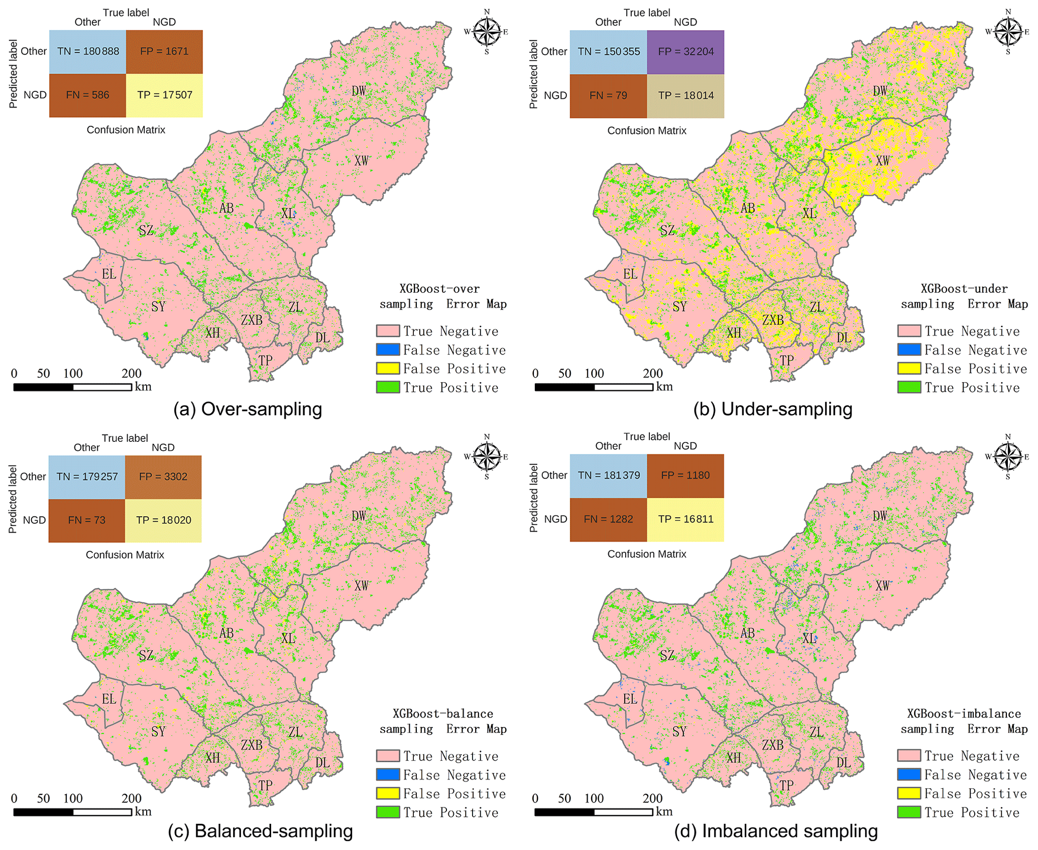
Figure 5 Error map of different sampling methods using the XGBoost model.

3.2 Driver selection

Figure 6 is a summary plot produced from the training dataset; it includes approximately 13 200 points (66 % of the sample size). This plot combines feature importance (drivers are ordered along the y axis) and driver effects (SHAP values on the x axis), which describe the probability of NGD having occurred. Positive SHAP values refer to a higher probability of NGD. The gradient colour represents the feature value from high (red) to low (blue), as previously introduced in Fig. 2. As Fig. 6 shows, disdense was the primary driver for NGD in the study region. The relationship between disdense and NGD is non-linear, which can be seen from the SHAP values being both positive and negative (black rectangle in Fig. 6). The interpretation of the effects of disdense can be summarised as a higher probability of NGD with increasing distance from dense grassland (see black rectangle in Fig. 6 with pink colour on the right).

Figure 6 shows that driver effects include both linear-dominated relationships, such as sheep, GDP, and others, and non-linear-dominated relations, such as disdense, dismode, and others. In addition, the figure shows that the most important drivers for NGD are the changes of distance to dense, moderately dense, and sparse grassland, then followed by sheep density and the distance to unused land. The effect of policies comes almost at the bottom, indicating that policies implemented outside sandy areas seem to have little effect on GD. The geographical factors DEM and slope are also positioned mid-field. The effect of geographical drivers does not appear to be as strong as the effect of other drivers. The change of distance to mining, located at the bottom for all drivers, does not have a strong effect on NGD compared to other drivers.

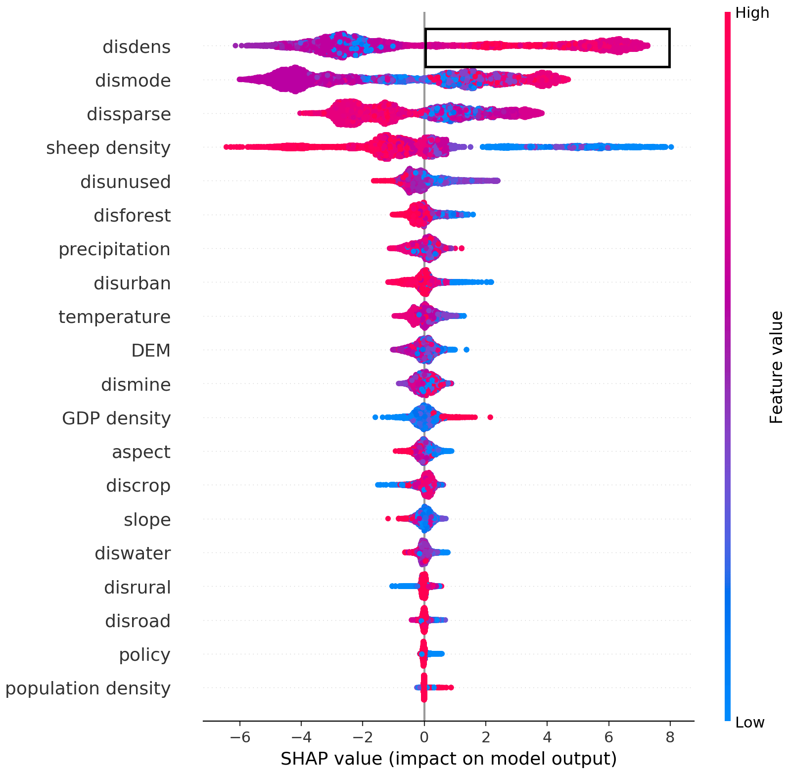
Figure 6 Driver ranking by SHAP values based on the training dataset (66 % of sample size) using the over-sampling method.

Note that the top rank indicates the most significant effects across all predictions. Each point in the cloud to the left represents a row from the original dataset. The colour code denotes high (red) to low (blue) feature values. Positive SHAP values represent a higher likelihood of NGD, while negative values indicate lower likelihoods. The range across the SHAP value space indicates the degradation probability, expressed as the logarithm of the odds.

A recursive attribute elimination method was performed to determine how attribute reduction affects modelling performance using XGBoost with the oversampling method (see Fig. S5; for more details, refer to Samardžić-Petrović et al., 2015). The results indicate that the first three drivers may already produce a satisfactory model (κ=0.74, AUC-PR = 0.85, recall = 0.92), while adding the fourth driver can produce a robust model (κ=0.94, AUC-PR = 0.98, recall = 0.98). This means that XGBoost used with the oversampling strategy can predict NGD with very high accuracy using a relatively small amount of data. Figure S6 shows the simulation result using the first four drivers and compares the results with the observed map.

3.3 Relationship between NGD and drivers in the XGBoost model

SHAP values and spread (Fig. 7) indicate that no linear relationship between driver and prediction could be found for any of the individual features. Change of distance to dense, moderately dense and sparse grass pixels, and change of sheep density were the dominant drivers for NGD. Figure 7a indicates that when disdense <0, the SHAP value is negative, and when the distance to dense grass areas is small, the likelihood of degradation is also small. The relationship seems to be more complex for distance to moderately dense grass (dismode; Fig. 7b); here, no simple linear interpretation is obvious. For distance to sparse grass (dissparse; Fig. 7c), the pattern again suggests a rather linear interpretation, which is that the likelihood of degradation increases with decreasing distance. For sheep density, Fig. 7d indicates that when sheep density decreased, the probability of GD obviously increased. Policy was not identified as a major driver of GD (Fig. 6). However, policy effects obviously have a different impact inside and outside sandy zones. Figure 7e shows that our initial assumption is invalid: the probability of GD increased inside the sandy areas where we assumed effective policy measures to be in place (value 0). This result is also in line with Fig. 7g, which shows that the closer an area is to unused land, the more likely it is that degradation will occur there.

We can identify three groups for the remaining 14 drivers. For GDP and population density (Fig. 7g and h), the likelihood of NGD increases with increasing values. Figure 7i–j indicate that warmer and drier climate conditions increase the probability of GD. Figure 7k, l, m, and n indicate that the probability of GD rises with closer distances to forest, urban, rural, and water areas. Figure 7o shows a slight SHAP value pattern, in which the closer to cropland, the more unlikely degradation will occur. This is mainly due to transformation from cropland to grassland. Figure 7p–t do not show any interpretable spatial pattern.

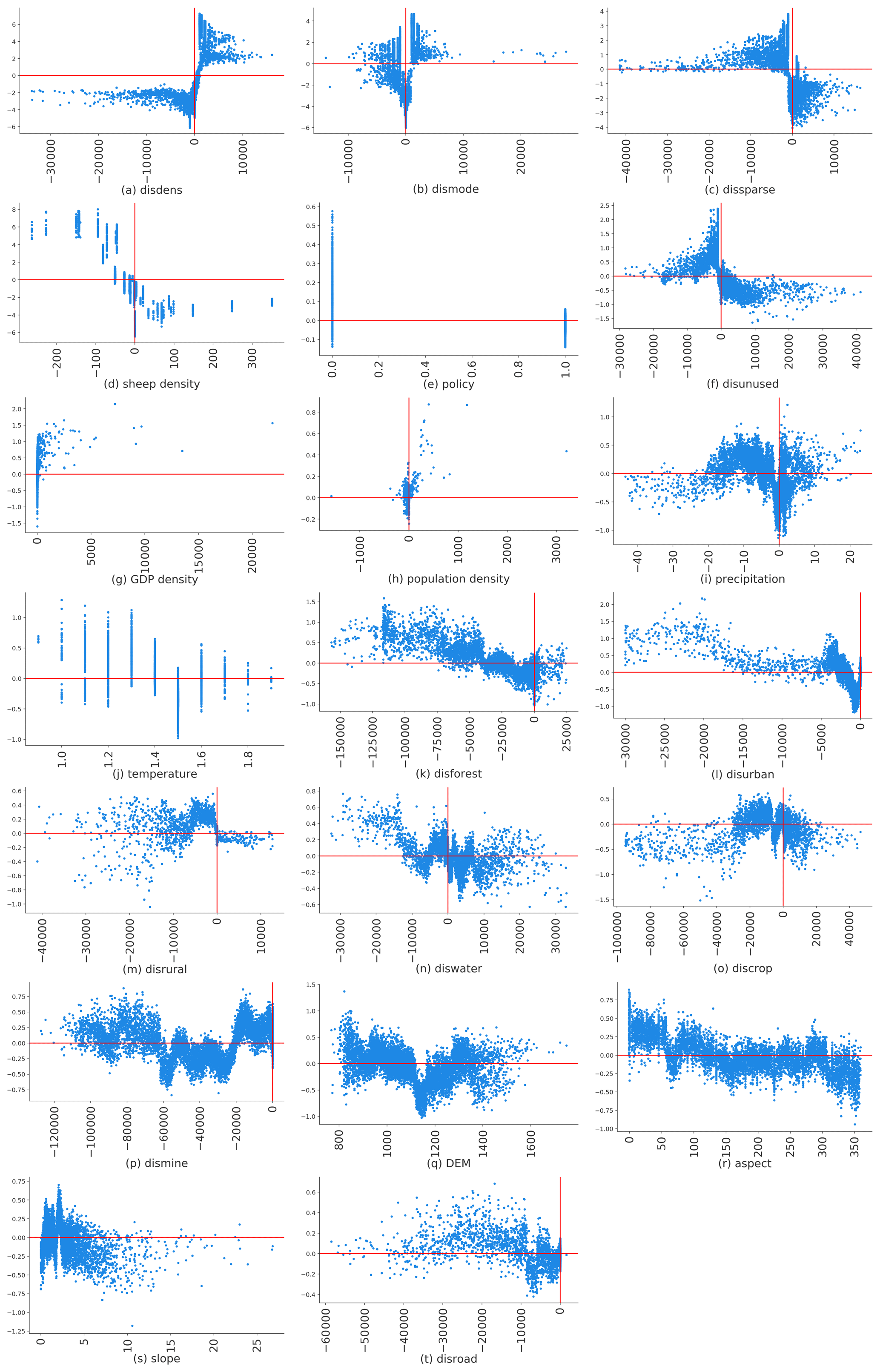
Figure 7 The SHAP dependence plot for each driver (the y axis is the SHAP value for each driver).

3.4 Mapping the primary drivers of NGD

All drivers' contributions to NGD were ranked according to their SHAP values for each pixel in this study. Figure 8 shows the primary driver for each NGD pixel. Distance to grassland pixels (dense, moderately dense, and sparse grass) were the major drivers of NGD, responsible for 9478, 3892, and 1629 NGD pixels, respectively. Sheep density was responsible for 3042 NGD pixels, ranking third among all drivers. This order differs to that in Figs. 6 and 8 because in those cases, ranking is based on the total contribution of all drivers. Figure S7 shows the number of NGD pixels in which a driver was dominant or primary. The change of distance to any type of grassland was the primary driver for about 82.8 % of the total NGD pixels; sheep density accounted for 16.8 %. The remaining seven drivers caused less than 1 % of the total NGD. We can see from the spatial pattern that the change of distance to grassland was the major driver for GD in the dense grassland region (counties of DW, XL, and AB), while in the counties of SZ, SY, ZXB, ZL, and TP, sheep density was often identified as the major driver.

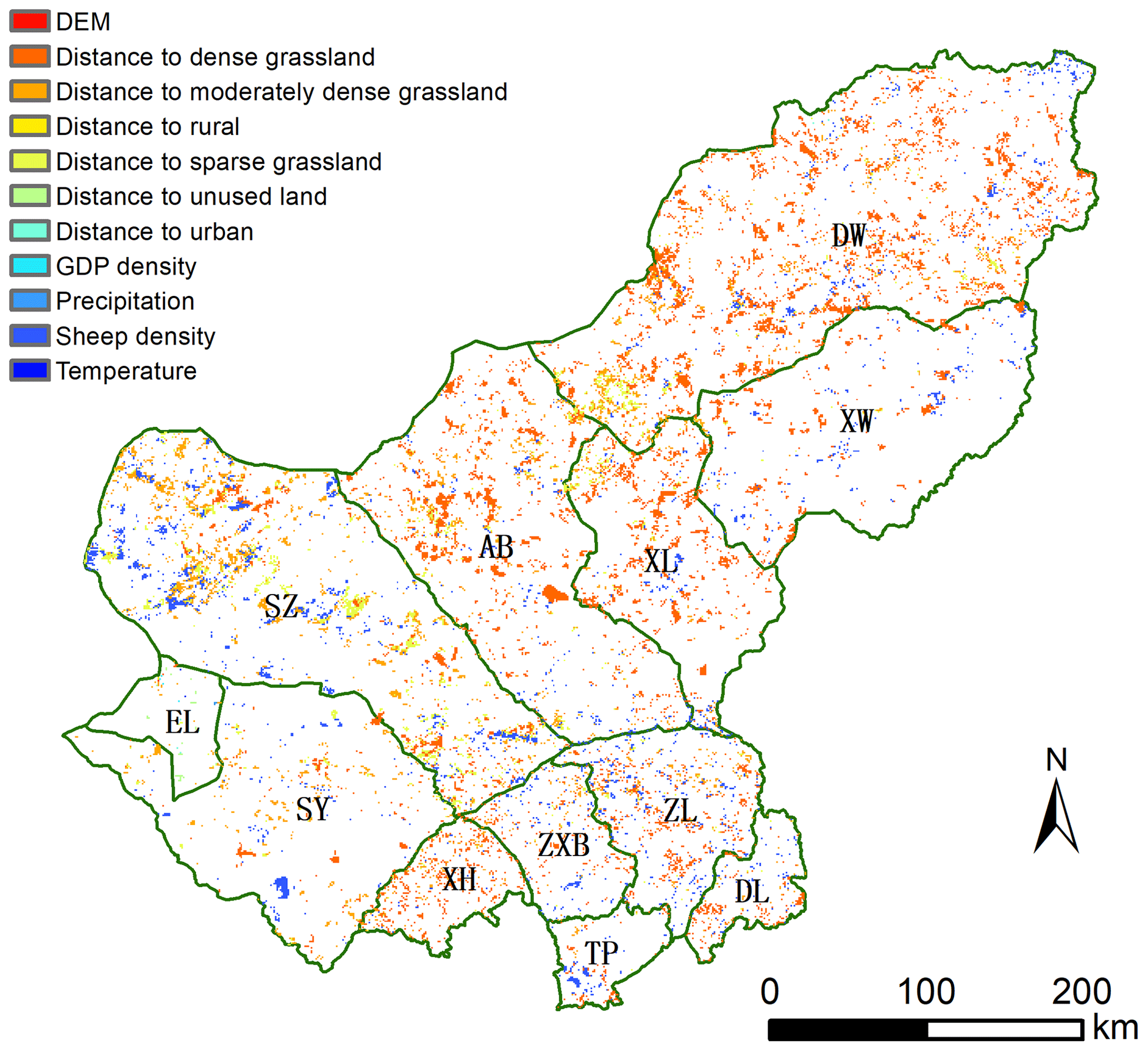
Figure 8 Spatial patterns of primary drivers for each pixel for NGD.

3.5 Regions of high risk for grassland degradation

A probability map of NGD was produced (Fig. 9). Low probabilities of NGD were found in the central and northern counties (DW, XL, AB, SZ, ZL ZXB, and XH), while high-probability regions were EL, SY, and XW. TP and DL in the south were categorised as low-probability regions, due to their lower share of grassland area.

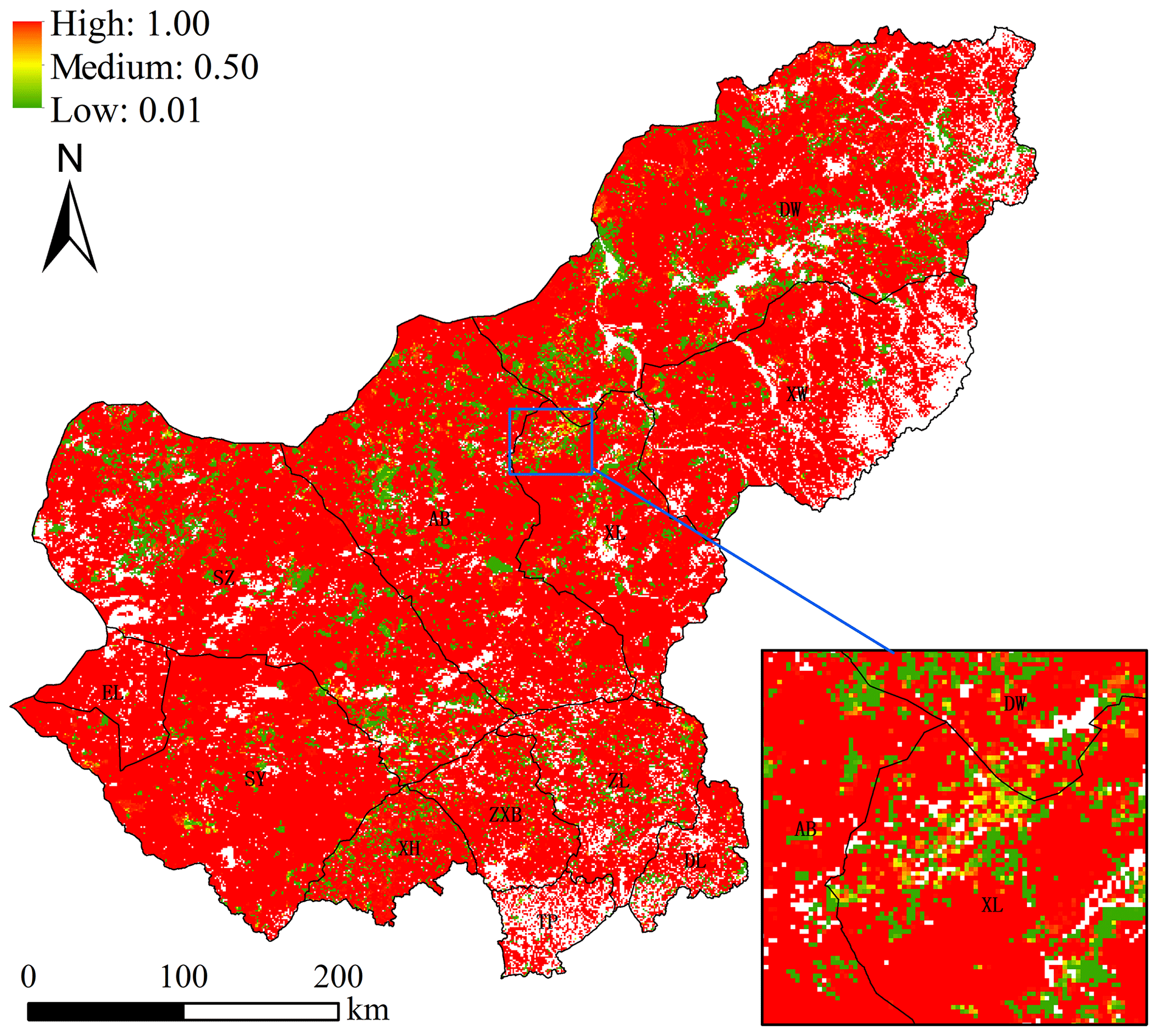
Figure 9 Degradation probability map for grassland in Xilingol, including a zoom into Xilinhot (XL) for more details. The probability is based on the four most important drivers.

4 Discussion

4.1 ML model building and evaluation

In this study, we defined a general framework for creating an ML model using the XGBoost algorithm for the purpose of analysing and predicting land-use change. XGBoost obtained a κ of 93 % and a recall value of >99 % when used to simulate and predict GD in this study. Compared to other popular ML learning algorithms, XGBoost exhibited a strong prediction ability. In studies where ANN, SVM, RF, CART, multivariate adaptive regression spline (MARS), or LR were used in combination with cellular automata (CA), the recall value is usually 54 %–60 % (Shafizadeh-Moghadam et al., 2017). Ahmadlou et al. (2019) stated that MARS and RF only yield high accuracy in training runs but do not prove to be very accurate in the validating process when simulating land-use change.

Concerning the four sampling strategies we used to test the imbalance issue, we found that all strategies performed satisfactorily in the training runs. In the simulation, the under-sampling strategy yielded a relatively low accuracy (κ=0.46) model. We assume that removal of data from the majority class causes the model to lose the important concepts pertaining to the majority class (He and Garcia, 2009). XGBoost used with the under-sampling method always produced similar results, irrespective of the size of the dataset (see Fig. S8). We conclude from this pattern that XGBoost is also able to use sparse data to reflect real-world problems (Chen and Guestrin, 2016).

4.2 SHAP values and drivers of grassland degradation

The general idea of introducing SHAP values as a further tool to analyse XGBoost ranking is to provide a method to evaluate the ranking with respect to causal relationships. The original XGBoost ranking is based on the in-built feature selection functions “Gain” (refers to the improvement in accuracy provided by a feature), “Weight” (or frequency, refers to the relative number of a feature occurrence in the trees of a model), and “Coverage” (refers to the relative numbers of observations related to this feature). However, these functions always produce different rankings of drivers (Abu-Rmileh, 2019) due to random components in the algorithms. SHAP values introduce two further properties of feature importance measures: consistency (whenever we change a model such that it relies more on a feature, the attributed importance for that feature should not decrease) and accuracy (the sum of all feature importance values should equate to the total importance of the model; Lundberg, 2018; Lundberg and Lee, 2017). Consistency is required to stabilise the ranking throughout the analysis, reducing the change of order in the ranking to a minimum when the number of identified drivers changes. The accuracy property of SHAP makes sure that each driver's contribution to overall accuracy remains the same, even when drivers are excluded from analysis. Other methods usually compensate for the withdrawal of a driver from the analysis, which makes the determination of a single driver's contribution difficult.

The feature ranking based on SHAP values indicated that the change of distance to any type of grassland (dense, moderately dense, and sparse grass) is the most important driver for any newly added grassland degradation. In this context, dense and moderately dense grassland areas are more easily degraded than other land-use types, followed by sparse grass. These results are in line with previous studies (Li et al., 2012; Xie and Sha, 2012). Good-quality grassland is more likely to be degraded through increasing human disturbance. An explanation for this can be derived from local people's living strategies. People who live in good-quality grassland areas are more likely to use grassland for livestock production with higher animal densities, risking overgrazing. Furthermore, Li et al. (2012) indicated that good-quality grassland is more likely to be converted to other land-use types, such as cropland. In contrast, people who have lived in sparse grassland regions for centuries have long adapted to low productivity, reducing their livestock numbers accordingly. They have also developed strategies to cope with variability in weather conditions, e.g. by preparing and storing more fodder and forage.

Sheep density was identified as the fourth major driver. However, the SHAP values indicate that when sheep density decreases, the probability of grassland degradation increases. Overgrazing has been the dominant driver for grassland degradation on the Mongolian plateau before, which has changed the grassland ecosystem significantly towards lower grass coverage (Nkonya et al., 2016; Wang et al., 2017). However, there is recent evidence that this causal relationship has changed. It now appears that farmers increasingly select their livestock numbers according to the carrying capacity of the grazing land (Cao et al., 2013b; Tiscornia et al., 2019b). By passing the “Fencing Grassland and Moving Users” policy (FGMU), the Chinese government issued a law that regulates livestock numbers based on a previously calculated carrying capacity. This development has upturned the causal relationship between livestock numbers and NGD, reflected by the SHAP value pattern in Fig. 6.

Besides the four main drivers, seven other drivers also occasionally appear as the main driver for some pixels (Fig. 8). This highlights the fact that, at the local level, other drivers apart from the four drivers identified as being major can also play a significant role. For example, in the county of EL, the remaining seven drivers were mainly responsible for NGD. EL has less NGD after 2000 compared with other counties in Xilingol (Fig. S1), and most of the EL area is covered by sparse grass. EL is the most frequented border control point to Mongolia and is subject to intensive tourism.

In the sparse grassland and agro-pastoral regions (SZ, SY, ZXB, ZL, and TP), sheep density was identified as the important driver. This indicates that, even though livestock numbers have decreased, grassland is still experiencing serious degradation in this region. Here we see additional potential for installing further grassland conservation measures, such as adjusting the livestock number to the grassland carrying capacity.

4.3 The current risk of grassland degradation in Xilingol

Three regions of different risk classes were identified in the probability map of NGD (Fig. 9). The low-risk region (DW, XL, AB, SZ, ZL ZXB, and XH) is dominated by good-quality grassland (dense and moderately dense grass). In recent decades, this region has suffered from increasing human disturbance, e.g. overgrazing and mining development. However, after 2000, grassland in this region has recovered, mainly as the result of ecological protection projects (Sun et al., 2017). Even though this region is predicted as being less exposed to the risk of land degradation in the future, attention is still required for the restoration process. The high-risk region includes the counties of EL, SY, and XW. EL and SY are covered by a large share of low-quality grassland, which – due to its own fragility – is likely to be affected by extreme climate and human disturbance, more than higher-quality grasslands for example. The recent change in grassland property rights and the establishment of ecological protection projects have also limited the mobility of nomadic herders throughout Xilingol. As a consequence, herders cannot easily change grazing spots if extreme weather occurs; they are then bound to have their cattle graze at the same spots, increasing the pressure on low-quality grasslands in particular (Qian, 2011). For a long time, fragile grassland remained in an equilibrium state with the extreme weather (frequent droughts, “dudz”) to which it was exposed, and with the nomadic livestock husbandry that the region's inhabitants practised. However, when the property rights of grassland and livestock were changed from collective to private, the nomadic lifestyle was largely abandoned.

4.4 The limitations of XGBoost for scenario exploration

XGBoost has already scored top in a range of algorithm competitions in the data science community (Kaggle, 2019) due to its high accuracy and speed (Chen and Guestrin, 2016). ML models extract patterns from data, without considering any existing expert knowledge, which is why they are increasingly used to identify non-linear relationships (Ahmadlou et al., 2016; Samardžić-Petrović et al., 2015; Tayyebi and Pijanowski, 2014b). However, ML models require specific data structures for each problem to which they are applied. In this study, we simulated grassland degradation in two different phases (1975–2000 and 2000–2015). All time series of driver data were organised as model inputs, while grassland degradation dynamics were organised as prediction targets. Although the model achieved high accuracy in predicting NGD in Phase 2, it was not possible to achieve acceptable results in simulating both Phase 1 and Phase 2 separately. Second, compared with conventional models, the XGBoost model cannot be easily transferred to other regions for the same research question. Models like CLUE-S and GeoSOS-FLUS have been widely used in different regions across the world (Fuchs et al., 2018; Liang et al., 2018b; Liu et al., 2017; Verburg et al., 2002). When ML models are used in other regions, driver data must be collected and structures adapted. Thirdly, ML models always need to learn sufficiently before they are able to make predictions. This requires a sufficient amount of data covering historical periods or different land-use change patterns.

XGBoost alone is unable to project any scenarios of land-use change based on historical data. However, the methodology presented here can be applied to quantify alternative scenarios produced using other approaches, such as conventional, rule-based models (Verburg et al., 2002) or cellular automata (Islam et al., 2018; Shafizadeh-Moghadam et al., 2017).

5 Conclusion

Machine learning and data-driven approaches are becoming more and more important in many research areas. The design and development of a practical land-use model requires both accuracy and predictability to predict future land-use change, a well-fitted model that reflects and monitors the real world (Ahmadlou et al., 2019). The method framework presented here for building an ML model and explaining the relationship between drivers and grassland degradation identified XGBoost as a robust data-driven model for this purpose. XGBoost showed higher accuracy in training and simulation compared to existing ML models. Combined with over-sampling, it slightly outperformed in the simulation process. The simulated map has a high agreement with the observed values (kappa = 93 %).

We identified six basic steps that should be included in ML model building, and they are also similar for other research applications (Kiyohara et al., 2018; Kontokosta and Tull, 2017; Subramaniyan et al., 2018). However, different validation measures can be introduced in both the training process and the simulation process. In this study, we tested different evaluation measures to evaluate the ML model, e.g. a typical confusion matrix to evaluate the training process, AUC-PR to evaluate the goodness of the ML model, and the kappa index to measure the degree of matching between observed and simulated values. These validation indicators consider both the research object and data characteristics. For example, when the data size is unbalanced, AUC-PR is a better choice than AUC-ROC (Brownlee, 2018; Davis and Goadrich, 2006; Saito and Rehmsmeier, 2015).

SHAP was introduced in this context to provide a causal explanation of the patterns identified by the ML model. In our case, SHAP was used to explain how drivers contribute to grassland degradation processes at the pixel and regional level, despite their non-linear relationship. According to the analysis, the distance to dense, moderately dense, and sparse grass and sheep density were the most important drivers that caused new grassland degradation in this region. In addition, individual SHAP values of sheep density indicated that the causal relationship between grassland degradation and livestock pressure has changed over time: the increase in sheep density was not the major driver for NGD in Phase 2 of the land degradation trajectory. Instead, the decrease in the grazing capacity of grassland caused a decrease in livestock numbers. The primary driver map of NGD provided a more detailed picture of NGD drivers for each pixel, as an important support for grassland management in the Xilingol region. The individual SHAP values of each driver may be an important prerequisite for rule-based scenario-building in the future.