An urban large-eddy-simulation-based dispersion model for marginal grid resolutions: CAIRDIO v1.0

The ability to achieve high spatial resolutions is an important feature for numerical models to accurately represent the large spatial variability of urban air pollution. On the one hand, the well-established mesoscale chemistry transport models have their obvious shortcomings due to the extensive use of physical parameterizations. On the other hand, obstacle-resolving computational fluid dynamics (CFD) models, although accurate, are still often too computationally intensive to be applied regularly for entire cities. The major reason for the inflated computational costs is the required horizontal resolution to meaningfully apply obstacle discretization, which is mostly based on boundary-fitted grids, e.g., the marker-and-cell method. In this paper, we present the new City-scale AIR dispersion model with DIffuse Obstacles (CAIRDIO v1.0), in which the diffuse interface method, simplified for non-moving obstacles, is incorporated into the governing equations for incompressible large-eddy simulations. While the diffuse interface method is widely used in two-phase modeling, this method has not been used in urban boundary-layer modeling so far. It allows us to consistently represent buildings over a wide range of spatial resolutions, including grid spacings equal to or larger than typical building sizes. This way, the gray zone between obstacle-resolving microscale simulations and mesoscale simulations can be addressed. Orographic effects can be included by using terrain-following coordinates. The dynamic core is compared against a standard quality-assured wind-tunnel dataset for dispersion-model evaluation. It is shown that the model successfully reproduces dispersion patterns within a complex city morphology across a wide range of spatial resolutions tested. As a result of the diffuse obstacle approach, the accuracy test is also passed at a horizontal grid spacing of 40 m. Although individual flow features within individual street canyons are not resolved at the coarse-grid spacing, the building effect on the dispersion of the air pollution plume is preserved at a larger scale. Therefore, a very promising application of the CAIRDIO model lies in the realization of computationally feasible yet accurate air-quality simulations for entire cities.

1 Introduction

The state of the art in urban-air-quality modeling now almost routinely encompasses the scales at which processes governing the atmospheric dispersion within the urban planetary boundary layer (PBL) are explicitly represented (Benavides et al., 2019; Croitoru and Nastase, 2018; Kadaverugu et al., 2019). The reasons for this increase in physical detail are manifold. On the one hand, even though PBL mixing processes are often parameterized to a large extent, the parameterizations themselves must rely on a sound physical basis, for which detailed large-eddy simulations (LESs) can be consulted (Noh and Raasch, 2003; Kanda et al., 2013). Direct benefits of more detailed numerical simulations include an increased ability to produce more representative air-quality forecasts for individual locations (Carlino et al., 2016) and the provision of high-resolution four-dimensional data for research purposes, e.g., source attribution (Fernández et al., 2019) and exposure risk assessment (Chang, 2016). Exposure-relevant air pollution concentrations at pedestrian level are subjected to a considerable and also complex spatiotemporal variability, as they are not only influenced by the relative location of pollution sources but also very importantly by the urban morphology and associated meteorological conditions (Birmili et al., 2013; Paas et al., 2016; Harrison, 2018). For an accurate simulation, it is thus not only key to explicitly represent the urban canopy features but also to consider the prevailing mesoscale meteorological conditions. Depending on the level of physical detail, a trade-off in the use of high-resolution numerical simulations is often their exclusive applicability in a limited area, which can be very restrictive. Hence, an active topic of research is dedicated to improve the numerical efficiency of high-resolution modeling tools and their incorporation into a larger modeling framework (Baik et al., 2009; Jensen et al., 2017; Kurppa et al., 2020). Commonly used multiscale approaches consist of nested domains and involve different types of models designed for a specific scale range. To address the global and regional scales, the use of chemistry transport models (CTMs) in combination with numerical weather prediction (NWP) models is a well-established practice. Examples of those coupled model systems include the Integrated Forecasting System with chemistry (C-IFS; Flemming et al., 2015), the Weather Research and Forecasting model with chemistry (WRF-Chem; Grell et al., 2005), the Community Multi-scale Air Quality model (CMAQ; Appel et al., 2017), the ICOsahedral Nonhydrostatic model with Aerosols and Reactive Trace gases (ICON-ART; Rieger et al., 2015), and the Consortium for Small-scale Modeling Multi-Scale Chemistry Aerosol Transport model (COSMO-MUSCAT; Wolke et al., 2004, 2012). In all of these models, subgrid-scale effects of temperature and moisture, as well as PBL dynamics, are parameterized. The influence of the urban canopy on the PBL in NWP models can be considered through sophisticated canopy parameterizations (Martilli et al., 2002; Schubert et al., 2012). The improvements of these so-called urbanized NWPs are substantially reflected in the modeled pollutant concentrations (Kim et al., 2015; Wang et al., 2019). Nevertheless, as the model domain does not allow for an explicit representation of buildings, the pollutants emitted at street level are diluted over the entire grid cell, which can considerably deviate from real conditions, where a large part of the physical volume may be impervious. As a result, pollutant concentrations modeled using NWP-based approaches are more representative of the urban background (Korhonen et al., 2019). Another practical limit to resolution and accuracy of NWP models arises from the use of parameterizations themselves. Using WRF, Haupt et al. (2019) observed that for horizontal grid spacings below the typical PBL height, numerical results can become spurious. Based on their findings, they recommend not to apply NWPs on the subkilometer scale without careful replacement of the used parameterizations. In PBL meteorology, the microscale seamlessly follows the lower limit of the mesoscale (super-kilometer range) (Stull, 1988; Rakai and Gergely, 2013). However, adopting the modeling perspective, there is a clear segregation of microscale and mesoscale. While the latter is constrained at the lower end of the resolution by the extensive use of parameterizations, attempting to model PBL processes directly with microscale approaches requires sufficiently fine grid spacings. The landscape of microscale models is diverse (Fallah-Shorshani et al., 2017; Brown, 2014; Hanna et al., 2006) and it reflects the difficulty of finding a compromise between computational resources and accuracy. Computational fluid dynamics (CFD) models can be seen as the microscale pedants to NWPs. Among them, LES approaches are the most accurate but expensive ones. LES models resolve the turbulent spectra up to the filter cut-off size (often equivalent to the grid size) and rely on simplistic subscale parameterizations only (e.g., Maronga et al., 2019). These two different approaches (extensive parameterization vs. explicit representation) are difficult to merge at the bridging scale range (few tens of meters to 1 km), for which reason Haupt et al. (2019) coined the keyword of “terra-incognita” to refer to the problem. An exemplary study, in which a LES model was applied for horizontal resolutions up to above 100 m, is given by Efstathiou et al. (2016). However, their simulations did not include an urban canopy, whose discretization would obviously require a much finer grid. In fact, to fully resolve the energy-dominant eddies within street canyons, a spatial resolution of 15–20 grid points over a typical obstacle dimension size is needed (Xie and Castro, 2006). This translates in a grid spacing of about 1 m for typically sized buildings. The use of such fine grids for entire city domains is still prohibitively expensive in LES modeling. For example, Wolf et al. (2020) used a grid spacing of 10 m in their cutting-edge research study to simulate air pollutant dispersion in Bergen, Norway, with the Parallelized Large-Eddy Simulation Model (PALM) model. While this spatial resolution, according to the argument above, does not ensure a LES model to be eddy resolving in every part of the domain, the preference of a physically based model over the more widely used parameterized models for this grid size (e.g., plume or street-canyon models) can nevertheless be a legitimate choice. Resolved physics can still be maintained outside the densely built urban canopy. Within the canopy, the dispersion pattern on a larger scale is mostly shaped by the channeling and blocking effects of buildings, which can be represented also with coarser grids.

In physical computing, it is well known that only a slight increase in the grid spacing results in large computational savings (e.g., models using explicit time integration ideally perform 16 times faster on the same domain using a grid with doubled grid spacings in all three dimensions). These computational savings could in turn be spent in larger physical domains for more comprehensive yet accurate urban-air-quality simulations. A key feature that sets the technical limits to the spatial resolution in urban boundary-layer modeling is the discretization method used for obstacles. A class of methods that allow for obstacle geometries not bound to the grid is the immersed boundary methods, summarized by Mittal and Iaccarino (2005). These are essentially Cartesian methods, but instead of relying on a commonly used marker-and-cell method (grid cells are assigned either to the building interiors or to the atmosphere), they represent rigid boundary conditions (e.g., Neumann boundary condition for pressure) on grid-cell faces not coinciding with the obstacle boundary. Among these methods, the so-called direct forcing uses the ghost-cell interpolation technique, where image points from adjacent interior ghost points are mirrored across the rigid boundary and interpolated using surrounding fluid nodes. While this method greatly enhances the flexibility in the choice of the grid size, it still suffers from the empirical nature in the selection of the interpolation nodes and the interpolation method itself. On the other hand, an equivalent boundary forcing can be more rigorously deduced from a two-phase flow model (Drew, 1983) by neglecting the restoring source terms. Treating one of the phases as an non-deformable solid, Kemm et al. (2020) derived a diffuse interface (DI) model for compressible fluids. One of the main advantages of their approach is the algorithmic simplicity, as the boundary-forcing term is analytically coupled to the DI, which is advected as a scalar. In this work, we adopt the basic idea of DI and implement diffuse obstacle boundaries (DOBs) in our new City-scale AIR dispersion model with DIffuse Obstacles (CAIRDIO v1.0), which will be used as a computationally feasible yet accurate downscaling tool for mesoscale air pollution fields over urban areas. DOBs allow buildings to be represented as diffuse features, and thus the flexibility in the choice of grid resolution can be greatly increased. A DOB is a simplified form of DI resulting from the static boundaries associated with buildings. A DOB is incorporated in the discrete differential operators by considering the conservation laws in a finite volume framework. The equations are then solved with standard methods on a Cartesian grid. To interpret our DOB approach from a physical point of view, it can be argued that the grid cells are interspersed with a porous and semi-permeable medium. Their detailed structure is only of concern insofar as it determines the mass and momentum budged at the grid level through two different types of interface fields. To the authors' knowledge, this approach has not been used for air-quality modeling so far, but very interestingly the concept of permeability finds application in geological science (Haga, 2011). In contrast to geometry-aligned discretizations, which preserve a high degree of accuracy near obstacle walls but require high resolutions, this approach is more suited for the integral aspect of building shapes and configurations at marginal resolutions. However, by increasing the grid resolution, the approach seamlessly transitions to a traditional obstacle-resolving Cartesian approach, as the interface eventually becomes sharply defined and imposes Neumann boundary conditions on the pressure.

The paper is organized as follows: Sect. 2 provides a detailed description of the model CAIRDIO, including the spatial discretization method. Section 3 contains numerical tests to demonstrate the diffuse obstacle discretization, the dynamic core, and the parallel scaling capabilities. In Sect. 4, we present a model-evaluation study by simulating a realistic wind-tunnel dispersion experiment. Finally, in Sect. 5, the benefits and limitations of the approach are summarized and concluded with an outlook for potential future applications.

2 Model description

2.1 Basic equations

The physical domain consists of an interspersed, stationary solid phase representing the buildings and a mobile fluid phase. The governing equations for the mobile phase are deduced from a simplified two-phase model by neglecting restoring forces. In a two-phase model, phase-fraction functions α₁, α₂ with $\mathrm{0}\le {\mathit{\alpha }}_{\mathrm{1}}\le \mathrm{1}$ and ${\mathit{\alpha }}_{\mathrm{1}}+{\mathit{\alpha }}_{\mathrm{2}}=\mathrm{1}$ are used to formulate the set of equations of both phases individually. The equation of motion of an incompressible phase is adopted from Drew (1983) (Eqs. 41, 45 therein). By setting the interfacial force density and surface tension to zero, the simplified momentum equation of the mobile phase (indicated with α₁) is written as

$$\begin{array}{}\text{(1)}& \begin{array}{rl}& {\partial }_t\left({\mathit{\alpha }}_{\mathrm{1}}\mathit{\rho }\mathit{u}\right)=-\mathrm{\nabla }\cdot \left({\mathit{\alpha }}_{\mathrm{1}}\mathit{\rho }\mathit{u}\otimes \mathit{u}\right)-{\mathit{\alpha }}_{\mathrm{1}}\mathrm{\nabla }\left({\mathit{\alpha }}_{\mathrm{1}}p\right)+p_{\mathrm{I}}\mathrm{\nabla }{\mathit{\alpha }}_{\mathrm{1}}\\ & +\mathrm{\nabla }\cdot \left({\mathit{\alpha }}_{\mathrm{1}}\mathbf{\text{T}}\right)+{\mathit{\alpha }}_{\mathrm{1}}\mathit{\rho }\mathit{b}.\end{array}\end{array}$$

Here, the 3-D velocity vector is denoted by u, and ρ is the density of air and p_I the interface pressure, which reflects Newton's third law of motion near a fixed wall. As in Kemm et al. (2020), p_I is assumed to be in equilibrium with the surrounding fluid pressure p. The stress tensor T contains the contributions from subscale and surface fluxes in LES averaging. In this model, the implicit approach is used for spatial filtering (Schumann, 1975). Viscous stresses are neglected due to the high Reynolds numbers typically encountered in atmospheric flows. The sum of external body forces b contains the gravitational force and inertial forces resulting in a rotating frame of reference. The interface in our case is static, as buildings do not respond to the flow. This makes it possible to multiply the equation of motion with ${\mathit{\alpha }}_{\mathrm{1}}^{-\mathrm{1}}{\mathit{\rho }}^{-\mathrm{1}}$ to obtain the tendency equation in single-flow denotation. The reference density ρ_ref is kept constant in time for an incompressible fluid. The full set of model equations reads

$$\begin{array}{}\text{(2)}& {\displaystyle }\begin{array}{rl}& {\partial }_t\mathit{u}=-{\mathit{\alpha }}_{\mathrm{1}}^{-\mathrm{1}}\mathrm{\nabla }\left({\mathit{\alpha }}_{\mathrm{1}}\mathit{u}\otimes \mathit{u}\right)-{\displaystyle \frac{\mathrm{1}}{{\mathit{\rho }}_{\mathrm{ref}}}}{\mathit{\alpha }}_{\mathrm{1}}^{-\mathrm{1}}{\mathit{\alpha }}_{\mathrm{1}}\mathrm{\nabla }p-{\mathit{\alpha }}_{\mathrm{1}}^{-\mathrm{1}}\mathrm{\nabla }\\ & \cdot \left({\mathit{\alpha }}_{\mathrm{1}}\mathbf{\text{T}}\right)-\mathit{f}\times \mathit{u}+\mathit{g}{\displaystyle \frac{{\stackrel{\mathrm{‾}}{\mathrm{\Theta }}}_v-{\mathrm{\Theta }}_{\mathrm{v}}}{{\stackrel{\mathrm{‾}}{\mathrm{\Theta }}}_v}},\end{array}\text{(3)}& {\displaystyle }{\mathit{\alpha }}_{\mathrm{1}}^{-\mathrm{1}}\mathrm{\nabla }\cdot \left({\mathit{\alpha }}_{\mathrm{1}}\mathit{u}\right)=\mathrm{0},\text{(4)}& {\displaystyle }{\partial }_t\mathrm{\Theta }=-{\mathit{\alpha }}_{\mathrm{1}}^{-\mathrm{1}}\mathrm{\nabla }\cdot \left({\mathit{\alpha }}_{\mathrm{1}}\mathit{u}\mathrm{\Theta }\right)+{\mathit{\alpha }}_{\mathrm{1}}^{-\mathrm{1}}\mathrm{\nabla }\cdot \left({\mathit{\alpha }}_{\mathrm{1}}{k}_{\mathrm{h}}\mathrm{\nabla }\mathrm{\Theta }\right)+{\mathit{\alpha }}_{\mathrm{1}}^{-\mathrm{1}}{S}_{\mathrm{\Theta }},\text{(5)}& {\displaystyle }\begin{array}{rl}& {\partial }_t{Q}_{\mathrm{v}}=-{\mathit{\alpha }}_{\mathrm{1}}^{-\mathrm{1}}\mathrm{\nabla }\cdot \left({\mathit{\alpha }}_{\mathrm{1}}\mathit{u}{Q}_{\mathrm{v}}\right)+{\mathit{\alpha }}_{\mathrm{1}}^{-\mathrm{1}}\mathrm{\nabla }\cdot \left({\mathit{\alpha }}_{\mathrm{1}}{k}_{\mathrm{h}}\mathrm{\nabla }{Q}_{\mathrm{v}}\right)\\ & +{\mathit{\alpha }}_{\mathrm{1}}^{-\mathrm{1}}{S}_{Q_{\mathrm{v}}},\end{array}\text{(6)}& {\displaystyle }{\mathrm{\Theta }}_{\mathrm{v}}=\mathrm{\Theta }\left(\mathrm{1}+\mathrm{0.61}{Q}_{\mathrm{v}}\right).\end{array}$$

In the momentum equation (Eq. 2), the body-force term is replaced by the Coriolis term, with the Coriolis parameter f for a mean geographic latitude, and the buoyancy term using the Boussinesq approximation. g is the gravity-acceleration vector in the local frame of reference and Θ_v the virtual potential temperature defined by Eq. (6). The overbar denotes the horizontal mean state. Equation (3) is the continuity equation derived in an analogous way to the momentum equation from the original formulation in Drew (1983). The transport equation for scalars, like the potential temperature Θ and specific humidity Q_v, contains source terms from parameterized surfaces fluxes. These have to be multiplied with ${\mathit{\alpha }}_{\mathrm{1}}^{-\mathrm{1}}$. The scalar field k_h is the eddy-diffusion coefficient for heat. Note that the combinations ${\mathit{\alpha }}_{\mathrm{1}}^{-\mathrm{1}}\mathrm{\nabla }\cdot {\mathit{\alpha }}_{\mathrm{1}}$ and ${\mathit{\alpha }}_{\mathrm{1}}^{-\mathrm{1}}{\mathit{\alpha }}_{\mathrm{1}}\mathrm{\nabla }$ can be identified as particular versions of the divergence and gradient operator, which incorporate diffuse boundaries. Using a staggered grid, the stencil of α₁ (face centered) differs from ${\mathit{\alpha }}_{\mathrm{1}}^{-\mathrm{1}}$ (volume centered), so that the terms do not cancel each other out.

2.2 Computational grid

The computation uses a structured Arakawa-C grid, with the velocity components being defined at the cell faces and scalar fields at the cell centers. Vertical coordinate transformation allows for a curvilinear grid in the physical space to be adapted to a smoothly varying terrain function:

$$\begin{array}{}\text{(7)}& \stackrel{\mathrm{̃}}{x}=x\text{,}\stackrel{\mathrm{̃}}{y}=y\text{,}\stackrel{\mathrm{̃}}{z}=z-h(x,y).\end{array}$$

Here, z is the mean sea level height and h(x,y) the terrain-height function. Elevated levels are simply given by adding a horizontally constant vertical increment to the first level.

The pressure gradient in terrain-following coordinates is modified to

$$\begin{array}{}\text{(8)}& \mathrm{\nabla }p=\stackrel{\mathrm{̃}}{\mathrm{\nabla }}p-\left[{\partial }_{x}h(x,y)+{\partial }_{y}h(x,y)\right]{\partial }_{z}p.\end{array}$$

The divergence operator is applied on the contravariant velocity components, which are parallel to the cell-face normal. In our simple case, only the vertical contravariant velocity component ω differs from the covariant non-transformed component. It is given by

$$\begin{array}{}\text{(9)}& \mathit{\omega }=w-{\partial }_{x}hu-{\partial }_{y}hv.\end{array}$$

Using Eq. (9), the advective tendency of a scalar q is written as

$$\begin{array}{}\text{(10)}& {\partial }_{t}q=-u{\partial }_{x}q-v{\partial }_{y}q-\left[w-u{\partial }_{x}h-v{\partial }_{y}h\right]{\partial }_{z}q.\end{array}$$

Similarly, the continuity equation in terrain-following coordinates follows from

$$\begin{array}{}\text{(11)}& {\partial }_{x}u+{\partial }_{y}v+{\partial }_z(w-{\partial }_{x}hu-{\partial }_{y}hv)=\mathrm{0}.\end{array}$$

Combining Eqs. (11) and (8), the metric terms in the Laplace operator are obtained, which is later needed for the pressure equation:

$$\begin{array}{ll}\text{(12)}& {\displaystyle }\mathrm{△}=& {\displaystyle }\stackrel{\mathrm{̃}}{\mathrm{△}}-{\partial }_x\left({\partial }_{x}h{\partial }_z\right)-{\partial }_y\left({\partial }_{y}h{\partial }_z\right)-{\partial }_z\left({\partial }_{x}h{\partial }_x\right){\displaystyle }& {\displaystyle }-{\partial }_z\left({\partial }_{y}h{\partial }_y\right)+{\partial }_z\left[({\partial }_{x}h{)}^{\mathrm{2}}{\partial }_z\right]+{\partial }_z\left[({\partial }_{y}h{)}^{\mathrm{2}}{\partial }_z\right].\end{array}$$

As u, v, and w are maintained as the prognostic model variables and g is invariant under the given coordinate transformation, no metric terms arise in the buoyancy term. However, the horizontal averaging of Θ_v is carried out on z isosurfaces. Therefore, Θ_v is remapped to an auxiliary vertical grid and the calculated tendency is remapped back to the computational grid.

2.3 Diffuse obstacle boundaries

The spatial discretization uses a finite volume method, which allows a consistent treatment of the diffuse obstacle boundaries. To consider the conservation of a scalar q within two partitioned phases, the Gauss theorem is formulated for a single grid-cell volume ΔV and its total surface area ∂ΔV:

$$\begin{array}{}\text{(13)}& \begin{array}{rl}& \underset{\mathrm{\Delta }V}{\int }{\partial }_t\left[q_{\mathrm{m}}{\mathit{\chi }}_{\mathrm{m}}+q_{\mathrm{s}}(\mathrm{1}-{\mathit{\chi }}_{\mathrm{m}})\right]\mathrm{d}{V}^{\prime }=\\ & -\underset{\partial \left(\mathrm{\Delta }V\right)}{\int }\left[{\mathit{\eta }}_{\mathrm{m}}\cdot {\mathit{u}}_{\mathrm{m}}{q}_{\mathrm{m}}+(\mathrm{1}-{\mathit{\eta }}_{\mathrm{m}})\cdot {\mathit{u}}_{\mathrm{s}}{q}_{\mathrm{s}}\right]\mathrm{d}{A}^{\prime }.\end{array}\end{array}$$

Here, subscript m refers to the mobile phase and subscript s to the solid phase for the building interior. A^′ and V^′ are formal integration variables. χ_m is the volume-fraction function of the mobile phase and η_m the area-fraction function, over which the flux of the mobile phase is integrated. As already mentioned, the stationary solid phase is dropped, as it is ${\partial }_t{\mathit{\chi }}_{\mathrm{m}}=\mathrm{0}$, ${\partial }_t{q}_{\mathrm{s}}=\mathrm{0}$ and u_s=0. This simplifies the conservation form and finally leads to the particular differential form of the transport equation for the mobile phase:

$$\begin{array}{}\text{(14)}& \begin{array}{rl}& {\partial }_t{q}_{\mathrm{m}}=-{\displaystyle \frac{\mathrm{1}}{{\mathit{\chi }}_{\mathrm{m}}\mathrm{\Delta }V}}\underset{\partial \left(\mathrm{\Delta }V\right)}{\int }{\mathit{\eta }}_{\mathbf{m}}\cdot {\mathit{u}}_{\mathrm{m}}{q}_{\mathrm{m}}\mathrm{d}A=\\ & -{\displaystyle \frac{\mathrm{1}}{{\mathit{\chi }}_{\mathrm{m}}}}\mathrm{\nabla }\cdot {\mathit{\eta }}_{\mathrm{m}}\left({\mathit{u}}_{\mathrm{m}}{q}_{\mathrm{m}}\right)=:-{\mathrm{\nabla }}_{\mathrm{m}}\cdot \left({\mathit{u}}_{\mathrm{m}}{q}_{\mathrm{m}}\right).\end{array}\end{array}$$

The subscript m was only briefly introduced here and will be dropped again, as only the mobile phase is of interest.

Using the Cartesian grid structure, the discrete flux divergence results from

$$\begin{array}{ll}\text{(15)}& {\displaystyle }\mathrm{\nabla }\cdot \mathit{F}={\displaystyle \frac{\mathrm{1}}{\mathit{\chi }\mathrm{\Delta }V}}& {\displaystyle }\left[\right({\mathit{\eta }}_x\mathrm{\Delta }{A}_x{F}_x{)}^{\mathrm{L}}-({\mathit{\eta }}_x\mathrm{\Delta }{A}_x{F}_x{)}^{\mathrm{R}}{\displaystyle }& {\displaystyle }+({\mathit{\eta }}_y\mathrm{\Delta }{A}_y{F}_y{)}^{\mathrm{L}}-({\mathit{\eta }}_y\mathrm{\Delta }{A}_y{F}_y{)}^{\mathrm{R}}\\ {\displaystyle }& {\displaystyle }+({\mathit{\eta }}_z\mathrm{\Delta }{A}_z{F}_z{)}^{\mathrm{L}}-({\mathit{\eta }}_z\mathrm{\Delta }{A}_z{F}_z{)}^{\mathrm{R}}],\end{array}$$

where ΔV and $\mathrm{\Delta }{A}_{x,y,z}$ are the cuboid volumes and face areas, respectively. The superscripts R and L refer to the left and right cell faces for each dimension, respectively. F_x, F_y, and F_z are fluxes whose concrete form is determined by the partial differential equation. Note that the contravariant flux has to be used for F_z.

The pressure-gradient components on the cell faces are discretized with second-order accuracy. The gradient components centered on the x- and z-oriented cell faces, respectively, are

$$\begin{array}{}\text{(16)}& {\displaystyle }\begin{array}{rl}& {\partial }_{x}p={\displaystyle \frac{\mathrm{2}{\mathit{\eta }}_x\mathrm{\Delta }{A}_x}{(\mathit{\chi }\mathrm{\Delta }V{)}^{\mathrm{L}}+(\mathit{\chi }\mathrm{\Delta }V{)}^{\mathrm{R}}}}\left(p^{\mathrm{R}}-p^{\mathrm{L}}\right)\\ & -{\displaystyle \frac{\mathrm{1}}{{\mathrm{\Delta }}_x}}\left(h^{\mathrm{R}}-h^{\mathrm{L}}\right){\mathbf{L}}^{z\to x}{\partial }_{z}p,\end{array}\text{(17)}& {\displaystyle }{\partial }_{z}p={\displaystyle \frac{\mathrm{2}{\mathit{\eta }}_z\mathrm{\Delta }{A}_z}{(\mathit{\chi }\mathrm{\Delta }V{)}^{\mathrm{L}}+(\mathit{\chi }\mathrm{\Delta }V{)}^{\mathrm{R}}}}\left(p^{\mathrm{R}}-p^{\mathrm{L}}\right),\end{array}$$

where L^z→x is the linear interpolation operator from a z face to an x face, and Δ_x is the cuboid size used for differencing the terrain function.

For a grid-conform surface, the area fractions ${\mathit{\eta }}_{x,y,z}=\mathrm{0}$, from which the required homogeneous zero Neumann boundary condition follows. In this case, a grid cell is completely surrounded by grid-conform surfaces and the pressure value inside is decoupled from any neighboring values, reflecting its physical meaninglessness. For partially open semi-permeable cell faces, the boundary condition is imposed on a fraction of the cell face area only.

The scaling fields ${\mathit{\eta }}_{x,y,z}$ and χ are derived from geometric building data. As an alternative to using terrain-following coordinates, it is possible to use diffuse boundaries for the terrain, in which case, the subsurface is also represented by a geometric shape. Per definition, the volume-fraction field χ is expressed as the fraction of the obstacle-free volume in each grid cell. For numerical reasons, however, χ is limited to a small non-zero value. For well-resolved buildings, the area-scaling fields ${\mathit{\eta }}_{x,y,z}$ are derived by calculating the intersections of the buildings with the grid-cell faces. For under-resolved buildings, however, this method fails to take the grid alignment into account. A resulting effect may be the entire missing of buildings if they do not intersect with a particular cell face but nevertheless block the flow within a grid cell. Figure 1a shows two possible scenarios, where grid cells are intersected by a building, which obviously blocks the flow in one dimension completely but does not intersect with the cell faces oriented in the direction of the blocking. In order to capture such occurrences more reliably, a modified method to calculate the area fractions is used. In this method, the grid-cell volume is partitioned in slices, with the slicing planes being displaced along the dimension considered (e.g., the x dimension for yz faces). The minimum value over the free-volume fractions of all slices is computed to define a cell-area-scaling factor, which is then assigned to the cell face in closer proximity to the obstacle. For a more robust capture of non-parallel building walls, the slicing can be repeated several times with a slight rotation of the plane normal. If, occasionally, a cell face is assigned to both values from the adjacent left and right grid cells, respectively, the minimum of both values is taken. For the resulting cell face left without assignment, the geometric intersection with buildings is calculated as in the resolved case. Figure 1b demonstrates that this method preserves the blocking effect of a triangular-shaped building for spatial resolutions, which are too coarse to resolve individual building walls.

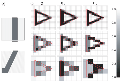
Figure 1 (a) Depiction of two different building sections (gray-filled areas) inside a grid cell. The black lines mark the effectively blocked area of the respective side. The line pattern symbolizes the slicing of the grid-cell volume, which is shown here only for the x dimension. (b) Scaling factors for a complete building, now depicted as fields calculated for three different grid resolutions. χ is the volume-scaling field, and η_x, η_y are the horizontal components of the area-scaling field.

2.4 Numerics

2.4.1 Advection scheme

The advective tendency for a scalar q is obtained by adding the remnant velocity-divergence term from the approximate pressure solution to the flux-divergence term of the conservation law (Eq. 15):

$$\begin{array}{}\text{(18)}& ({\partial }_{t}q{)}_{\mathrm{adv}}=-\mathrm{\nabla }\cdot \left(\mathit{u}q\right)+q\mathrm{\nabla }\cdot \mathit{u}.\end{array}$$

The flux components are linear and given by the product of the reconstructed values $\stackrel{\mathrm{̃}}{q}$ at cell faces and the exactly given momentum components. We use an upwind-biased stencil of fifth order, which results in two reconstructions (${\stackrel{\mathrm{̃}}{q}}^{+}$ and ${\stackrel{\mathrm{̃}}{q}}^{-}$) on each cell face. For an x-oriented face, the reconstructions are merged to the numerical flux by considering the wind direction:

$$\begin{array}{}\text{(19)}& {\left(uq\right)}_x=\mathrm{0.5}\left[u_x({\stackrel{\mathrm{̃}}{q}}^{+}+{\stackrel{\mathrm{̃}}{q}}^{-})-\left|\right|u_x\left|\right|({\stackrel{\mathrm{̃}}{q}}^{+}-{\stackrel{\mathrm{̃}}{q}}^{-})\right].\end{array}$$

For non-uniform grid spacings, the coefficients of the reconstruction polynomials are precomputed from the spatial derivative of the Lagrange polynomial which interpolates the primitive function at cell faces (see, e.g., Shu, 1998). We use the pseudo-grid spacing calculated by ${\mathrm{\Delta }}_x^{\mathrm{eff}}=\mathrm{2}{\mathrm{\Delta }}_x\mathit{\chi }/({\mathit{\eta }}_x^{\mathrm{L}}+{\mathit{\eta }}_x^{\mathrm{R}})$ instead of the computational grid spacing in order to automatically adjust the effective stencil width near obstacle boundaries. The behavior of the pseudo-grid-based reconstruction of maximum fifth order is demonstrated in Fig. 2 for a positive flow direction (left to right). Within the shown circular obstacle, the pseudo-grid spacing tends toward infinity, which effectively excludes such decoupled cells from interpolation. The resulting smaller stencils can be downwind biased. An effective measure to prevent numerical instabilities is the application of a flux limiter (e.g., from Sweby, 1984) near obstacle boundaries. To avoid non-physical results of positive scalars, a limiter has to be applied anyway. In the case of momentum advection, we use the absolute difference $\left|{\mathit{\eta }}_x\right(j-\mathrm{1})-{\mathit{\eta }}_x(j\left)\right|$ as a weighting function to merge the limited and unlimited reconstructions for obstacle-specific limiting. Note that this expression is upwind-biased (assuming a positive wind direction). In the free boundary layer, the difference is zero and no limiting is applied. The routine for scalar cell-centered advection is repeatedly used to advect a left-faced u^l and right-faced value u^r for each momentum component (Hicken et al., 2005; Jähn et al., 2015), resulting in a total of six advection steps. The final momentum tendencies are obtained by interpolation of two centered tendencies on the face:

$$\begin{array}{}\text{(20)}& {\partial }_t^{\mathrm{adv}}u={\displaystyle \frac{{\left(\mathit{\chi }\mathrm{\Delta }V{\partial }_t^{\mathrm{adv}}{u}^{\mathrm{l}}\right)}^{\mathrm{R}}+{\left(\mathit{\chi }\mathrm{\Delta }V{\partial }_t^{\mathrm{adv}}{u}^{\mathrm{r}}\right)}^{\mathrm{L}}}{(\mathit{\chi }\mathrm{\Delta }V{)}^{\mathrm{R}}+(\mathit{\chi }\mathrm{\Delta }V{)}^{\mathrm{L}}}}.\end{array}$$

Spatial accuracy of momentum advection is limited to the order of this interpolation procedure, which is of second order here.

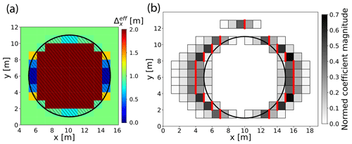
Figure 2 (a) Plot of the pseudo-grid spacing ${\mathrm{\Delta }}_x^{\mathrm{eff}}$ computed for a solid cylinder with diameter of 10 m using a uniformly constant grid spacing of 1 m. Decoupled cells inside the cylinder are characterized by ${\mathrm{\Delta }}_x^{\mathrm{eff}}>\mathrm{2}$ m in this plot. (b) Using same ${\mathrm{\Delta }}_x^{\mathrm{eff}}$ of (a), the reconstruction coefficients are computed for a five-point upwind-biased stencil. The absolute values of the reconstruction coefficients are re-normed to 1 and depicted in shades of gray at individual reconstruction sites, which are marked by a vertical red bar. Stencil points are rendered invisible for values below 10⁻⁴ and as such have a negligible influence on the reconstructed value.

2.4.2 Model integration

In the incompressible-flow equations, the pressure-gradient term is not directly coupled to a prognostic pressure equation. The projection method of Chorin (1968) is used to split the solution procedure in two steps. The first step integrates all the momentum tendencies, except the stated pressure-gradient term, explicitly in time to obtain a predicted velocity $\stackrel{\mathrm{̃}}{\mathit{u}}$:

$$\begin{array}{}\text{(21)}& \stackrel{\mathrm{̃}}{\mathit{u}}={\mathit{u}}_{t_{\mathrm{0}}}+({\partial }_t\mathit{u}{)}_{\mathrm{ex}}{|}_{t_{\mathrm{0}}}\mathrm{\Delta }t.\end{array}$$

The final velocity estimate after one integration step ${\mathit{u}}_{t_{\mathrm{1}}}$ has to fulfill the continuity equation:

$$\begin{array}{}\text{(22)}& \mathrm{\nabla }\cdot {\mathit{u}}_{t_{\mathrm{1}}}=\mathrm{0}.\end{array}$$

The required corrective tendency has to be associated with the neglected pressure gradient, which is formally integrated with an Euler-backward step to obtain the final velocity at $t_{\mathrm{1}}=t_{\mathrm{0}}+\mathrm{\Delta }t:$

$$\begin{array}{}\text{(23)}& {\mathit{u}}_{t_{\mathrm{1}}}=\stackrel{\mathrm{̃}}{\mathit{u}}-{\displaystyle \frac{\mathrm{\Delta }t}{{\mathit{\rho }}_{\mathrm{ref}}}}\mathrm{\nabla }|p_{t_{\mathrm{1}}}.\end{array}$$

By applying the divergence operator on both sides and requiring that $\mathrm{\nabla }\cdot {\mathit{u}}_{t_{\mathrm{1}}}=\mathrm{0}$, the well-known Poisson equation for pressure is obtained:

$$\begin{array}{}\text{(24)}& {\displaystyle \frac{{\mathit{\rho }}_{\mathrm{ref}}}{\mathrm{\Delta }t}}\mathrm{\nabla }\cdot \stackrel{\mathrm{̃}}{\mathit{u}}=\mathrm{△}p{|}_{t_{\mathrm{1}}}.\end{array}$$

After algebraic solution of this equation, the final state can now be composed of the fractional tendencies:

$$\begin{array}{}\text{(25)}& {\mathit{u}}_{t_{\mathrm{1}}}={\mathit{u}}_{t_{\mathrm{0}}}+\mathrm{\Delta }t\left[({\partial }_t\mathit{u}{)}_{\mathrm{ex}}{|}_{t_{\mathrm{0}}}-{\displaystyle \frac{\mathrm{1}}{{\mathit{\rho }}_{\mathrm{ref}}}}\mathrm{\nabla }p{|}_{t_{\mathrm{1}}}\right].\end{array}$$

Equation (25) is only first-order accurate in time. For higher accuracy, it is instead used a third-order strong-stability-preserving Runge–Kutta scheme (SSP-RK3) for the advective and pressure-gradient tendencies, which also allows us to use larger time steps. The pressure to correct the first two intermediate states is extrapolated from values given at previous time steps, and only for the final stage, the pressure solver is applied (Karam et al., 2019). We found that this combination supports stable integration up to a Courant number of C=0.7.

2.4.3 Pressure solution

The discretization of the Laplace operator P in the Poisson equation (Eq. 24) is obtained by the product of the discrete divergence D and gradient in sparse matrix form. D is defined by the flux balance in Eq. (15). Combining the operators to the pressure equation, the following sparse linear system is obtained:

$$\begin{array}{}\text{(26)}& \mathbf{\text{P}}p={\displaystyle \frac{\mathrm{1}}{\mathrm{\Delta }t}}\mathbf{\text{D}}\stackrel{\mathrm{̃}}{u}=:b,\end{array}$$

where $\stackrel{\mathrm{̃}}{u}$, p, and b are the one-dimensional expanded arrays of the corresponding structured fields. Equation (26) is solved with a geometric multigrid method in parallel using domain decomposition in two dimensions. The multigrid algorithm consists of applying a smoothing method of choice which is accelerated by coarse-grid corrections. Therefore, a hierarchy of coarse grids is employed (Brandt and Livne, 2011). A 3-D coarsening of the grid is carried out by agglomeration of eight grid cells to form a coarse-grid cell of the next-level grid. For uneven grid sizes, a plane of grid cells with respective orientation is left uncoarsened. This particular multigrid used in combination with finite volume discretizations is often referred to as a cell-centered multigrid in literature (Mohr and Wienands, 2004). Particular challenges to the multigrid algorithm include grid stretching and, in our case, non-smoothly varying coefficients associated with the diffuse boundaries, both resulting in coefficient anisotropy. An odd grid size results in coefficient anisotropy of the coarse-grid operators. In such cases, plane smoothers are often much more robust than their point-wise pendants (Llorente and Melson, 2000). Nevertheless, most of the difficulties could be overcome by applying less elaborate methods in the current model. Based on smoothing analysis, Larsson et al. (2005) give a condition for the optimal location of an uncoarsened plane in the case of an odd grid size. Galerkin coarse-grid approximation can result in a better approximation of the coarse-grid operator in this case, while discretization coarse-grid approximation can be more efficient for even-sized grid dimensions. Our algorithm employs a combination of both methods on different grid levels.

Yavneh (1996) found that for smoothing, successive over-relaxation (SOR) is generally superior to Gauss–Seidel smoothing (even for isotropic coefficients), and he also derived approximately optimal over-relaxation factors for SOR with red–black ordering applied in multigrid for the solution of anisotropic elliptic equations. In our implementation, also sparse-approximate inverse (SPAI) matrices (Tang and Wan, 2000; Bröker and Grote, 2001; Sedlacek, 2012) are available as suitable alternatives to SOR. These smoothers can inherently consider coefficient anisotropy through the algebraic method by which they are derived. Moreover, a variable number of non-zeros in the matrix allows a flexible control of the approximation quality and smoothing efficacy.

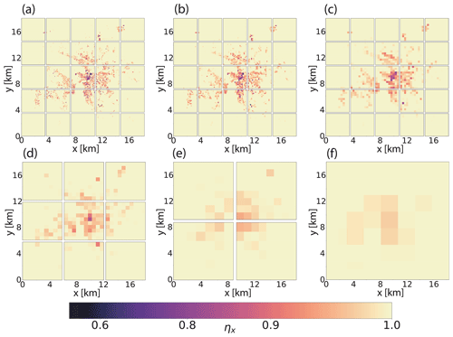
Figure 3 Example of a horizontal multigrid domain decomposition involving six grid levels. Depicted are the area-scaling factors of yz faces for the city of Leipzig at resolutions of (a) 80, (b) 160, (c) 320, (d) 640, (e) 1280, and (f) 2560 m. The scaling factors are needed in the discretization of the Poisson equation. On the coarsest grid, a single processor is left for the computation.

2.4.4 Lateral boundary conditions

Before each pressure correction step, lateral boundary conditions of the intermediate velocity field $\stackrel{\mathrm{̃}}{\mathit{u}}$ are updated. The update has to ensure global mass conservation:

$$\begin{array}{}\text{(27)}& \underset{\partial V}{\oint }{\displaystyle \frac{{\mathit{\rho }}_{\mathrm{ref}}}{\mathrm{\Delta }t}}\stackrel{\mathrm{̃}}{\mathit{u}}\cdot \mathit{n}\mathrm{d}{A}^{\prime }=\mathrm{0}.\end{array}$$

This expression implies a homogeneous-zero Neumann boundary condition for pressure at all lateral boundaries, as the already updated boundary values should not be changed by the projection:

$$\begin{array}{}\text{(28)}& \mathrm{0}={\mathit{\rho }}_{\mathrm{ref}}{\displaystyle \frac{\partial \stackrel{\mathrm{̃}}{\mathit{u}}}{\partial t}}\cdot \mathit{n}=\mathrm{\nabla }p\cdot \mathit{n}.\end{array}$$

Here, n is the unit normal vector on the boundary surface. A more general case arises with the use of terrain-following coordinates. By requiring not only ${\partial }_t\mathit{\omega }=\mathrm{0}$ but additionally ${\partial }_{t}w=\mathrm{0}$ at the bottom and top of the computation domain, the following boundary condition follows at these boundaries:

$$\begin{array}{ll}\text{(29)}& {\displaystyle }{\partial }_{z}p& {\displaystyle }=\mathrm{0}{\displaystyle }{\partial }_{x}p& {\displaystyle }=\left\{\begin{array}{ll}\mathrm{0}& {\partial }_{x}h\ne \mathrm{0}\\ \text{not specified}& \text{else}\end{array}\right.\\ \text{(30)}& {\displaystyle }{\partial }_{y}p& {\displaystyle }=\left\{\begin{array}{ll}\mathrm{0}& {\partial }_{y}h\ne \mathrm{0}\\ \text{not specified}& \text{else}.\end{array}\right.\end{array}$$

In the discrete gradient operator, homogeneous Neumann boundary conditions are implemented by setting all coefficients associated with the node to zero where the condition applies.

The boundary condition for the velocity field has to be compatible with a dynamic mesoscale forcing and also satisfy Eq. (27). Firstly, inflow and outflow regions are dynamically determined in order to impose separate appropriate boundary conditions. Outflow regions are characterized by convective transport out of the domain. Therefore, a simple normalized convective transport speed ($C_{⟂}=\frac{\mathrm{\Delta }t}{\mathrm{\Delta }x}\mathit{u}\cdot \mathit{n}$) is computed. Note that more elaborate formulations for C_⟂ exist. C_⟂ is further bounded to [0,1] for numerical reasons. It is then $C_{⟂}>\mathrm{0}$ for outflow regions. For such regions, the radiation boundary condition by Miller and Thorpe (1981) is imposed:

$$\begin{array}{}\text{(31)}& {\mathit{u}}_{l+\mathrm{1}}^{t+\mathrm{1}}={\mathit{u}}_{l+\mathrm{1}}^t-C_{⟂}\left({\mathit{u}}_{l+\mathrm{1}}^t-{\mathit{u}}_l^t\right).\end{array}$$

The order of the spatial indexing l is in normal direction to the boundary and not to be mixed up with the standard interior indexing. The index l+1 corresponds to the first ghost cell. At the remaining inflow boundaries, Dirichlet conditions are specified.

Instead of this flexible inflow–outflow boundary condition, a Rayleigh damping layer can be used as another prognostic tendency near the domain top:

$$\begin{array}{}\text{(32)}& {\partial }_t^{\mathrm{dmp}}q=-{\displaystyle \frac{R\left(z\right)}{\mathit{\tau }}}(q-q_{\mathrm{0}}).\end{array}$$

Equation (32) can be applied to gradually relax any prognostic variable toward a prescribed horizontal mean state at the top boundary. R is a ramp function with values between [0,1], τ the damping timescale, and q₀ the prescribed boundary value.

Final mass conservation is enforced by making sure that the total inflow–mass flow is exactly balanced by the total outflow–mass flow. This is accomplished by computing an averaged correction velocity from the mass-flow difference. In the case, each spatial dimension is considered independently from each other, this results in three different correction velocities. The correction velocities are finally added to the boundary-perpendicular velocity component at the outflow regions.

Figure 4 shows that the outflow boundary condition with the proposed convective transport speed is well suited to our incompressible model even for highly unsteady flows, like the depicted vortex street in the wake of a cylinder. Individual vortices are not visibly reflected at the boundary, and also in the temporal mean, based on Fig. 4b), the influence of the boundary is not noticeable. The flexible boundary condition can principally be applied to any other scalar quantity, although, specifying Dirichlet conditions for advected scalars was found to be well suited.

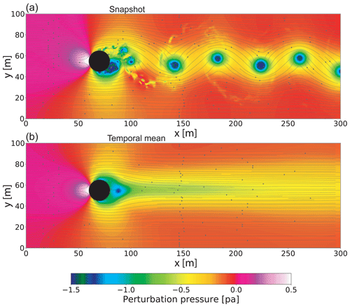
Figure 4 LES of 3-D flow past a cylinder. The horizontal grid spacing is uniformly 0.5 m. The cylinder has a diameter of 40 m. The approaching flow is laminar with u=1 m s⁻¹. Flexible Dirichlet-radiation conditions are imposed on all horizontal domain boundaries, while periodic boundary conditions are used in the z direction. The contour plot depicts the pressure and the streamlines the horizontal velocity field. Panel (a) shows a frame at the instance during a sharply defined vortex is about to cross the right boundary; panel (b) shows the temporal mean over a representative simulation period.

2.5 Physical processes

2.5.1 Subgrid model

For numerical simplicity and efficiency, a static Smagorinsky subgrid model is used (Deardorff, 1970). Since the atmospheric model is operated in the limit of infinite Reynolds numbers, the principal purpose of the subgrid model is to dissipate enough energy at the shortest wavelengths to obtain a physically realistic energy cascade. In our case, the subgrid model also has to compensate for the under-resolved vertical mixing of tracers within the urban boundary layer. In the Smagorinsky model, the rates of strain s_x,y are approximated by the velocity gradients:

$$\begin{array}{}\text{(33)}& s_{x,y}={\displaystyle \frac{\mathrm{1}}{\mathrm{2}}}\left({\partial }_{y}u+{\partial }_{x}v\right).\end{array}$$

The subscripts x, y refer to the spatial components. The turbulent fluxes are derived in analogy to the viscous fluxes by assuming an eddy viscosity ϵ_k:

$$\begin{array}{}\text{(34)}& u_x^{\prime }{u}_y^{\prime }=\mathrm{2}{\mathit{ϵ}}_{x,y}{s}_{x,y}.\end{array}$$

The often additionally mentioned anisotropic residual-stress tensor is ignored in the given incompressible case. In the most simple case, ϵ_x,y is also diagnosed from the rates of strain. ϵ_x,y is denoted in tensor form, as an anisotropic mixing length l_x,y is used to reflect grid anisotropy:

$$\begin{array}{}\text{(35)}& {\mathit{ϵ}}_{x,y}=l_{x,y}^{\mathrm{2}}\left|\mathbf{\text{S}}\right|f={\left(c_{\mathrm{s}}{\mathrm{\Delta }}_{x,y}\right)}^{\mathrm{2}}\left|\mathbf{\text{S}}\right|f_{\mathrm{s}}.\end{array}$$

$\left|\mathbf{\text{S}}\right|$ is the Frobenius norm of the strain-rate tensor. c_s is the Smagorinsky constant, which is fixed in a static model. Tests with a boundary-layer simulation revealed that the range $\mathrm{0.1}<c_{\mathrm{s}}<\mathrm{0.15}$ gives good results in combination with the fifth-order upwind scheme. Grid anisotropy enters via Δ_x,y, which is further modified by half the mean distances to walls h_x and h_y, respectively:

$$\begin{array}{}\text{(36)}& {\mathrm{\Delta }}_{x,y}=min\left(\sqrt{{\mathrm{\Delta }}_x{\mathrm{\Delta }}_y},\mathrm{1.8}{h}_x,\mathrm{1.8}{h}_y\right).\end{array}$$

Function f_s introduces the influence of the stratification on the eddy viscosity. It is assumed that

$$\begin{array}{}\text{(37)}& f_{\mathrm{s}}=\left\{\begin{array}{ll}\mathrm{0}& Ri\ge \mathrm{0.25}\\ \sqrt{\mathrm{1}-\mathrm{16}Ri}& Ri<\mathrm{0}\\ {\left(\mathrm{1}-\mathrm{4}Ri\right)}^{\mathrm{4}}& \text{else},\end{array}\right.\end{array}$$

with the Richardson number Ri:

$$\begin{array}{}\text{(38)}& Ri={\displaystyle \frac{g{\partial }_z{\mathrm{\Theta }}_{\mathrm{v}}}{{\mathrm{\Theta }}_{\mathrm{v}}|S{|}^{\mathrm{2}}}}.\end{array}$$

For scalar diffusion, the eddy viscosity is divided by the turbulent Prandtl number, which is assumed to be $Pr=\mathrm{2}/\mathrm{3}$ here.

If not mentioned otherwise, the appearing spatial derivatives are discretized with second-order differences. To obtain the strain-rate components and the eddy viscosity on different stencil points (cell faces areas and cell centers), linear interpolation is used. The subgrid tendency is formed by the divergence of the diffusive fluxes. Shifted grids are introduced to account for the definition of the velocity components on the cell faces. For example, diffusion of the u component requires a grid shifted by ${\mathrm{\Delta }}_x/\mathrm{2}$, for which the scaling fields are also obtained by linear interpolation. The diffusive fluxes are given by

$$\begin{array}{}\text{(39)}& F_{x,y}=\mathrm{2}{\mathit{ϵ}}_{x,y}{s}_{x,y}.\end{array}$$

For diffusion of the u component, the fluxes in the three spatial directions are F_x,x, F_x,y, and F_x,z. Those of the other components are obtained by permuting the subscripts. For a scalar quantity q, the required fluxes are F_x,x, F_y,y, and F_z,z, with the rates of strain being replaced by the gradient components.

2.5.2 Surface fluxes

Surface fluxes for momentum, heat and moisture are parameterized using Monin–Obukhov similarity theory (Louis, 1979). An expression for the vertical transfer coefficient C_z can be obtained by transforming the logarithmic wind law:

$$\begin{array}{}\text{(40)}& C_z={\displaystyle \frac{k^{\mathrm{2}}}{{\log }^{\mathrm{2}}(z/z_{\mathrm{0}})}}.\end{array}$$

k=0.4 is the Von Kármán constant, z₀ the surface roughness length, and z the height difference from the modeled surface to the grid level where the parameterization is evaluated.

The momentum sinks from horizontal surfaces are

$$\begin{array}{}\text{(41)}& {\displaystyle \frac{\partial u^{\prime }{w}^{\prime }}{\partial z}}=-{\displaystyle \frac{A_z}{\mathrm{\Delta }V}}{f}_{\mathrm{m}}{C}_{z}u\sqrt{u^{\mathrm{2}}+v^{\mathrm{2}}}\end{array}$$

and

$$\begin{array}{}\text{(42)}& {\displaystyle \frac{\partial v^{\prime }{w}^{\prime }}{\partial z}}=-{\displaystyle \frac{A_z}{\mathrm{\Delta }V}}{f}_{\mathrm{m}}{C}_{z}v\sqrt{u^{\mathrm{2}}+v^{\mathrm{2}}}.\end{array}$$

Analogously, the source terms for heat and moisture from horizontal surfaces are

$$\begin{array}{}\text{(43)}& {\displaystyle \frac{\partial {\mathrm{\Theta }}^{\prime }{w}^{\prime }}{\partial z}}=-{\displaystyle \frac{A_z}{\mathrm{\Delta }V}}{f}_{\mathrm{h}}{C}_z\left(\mathrm{\Theta }-{\mathrm{\Theta }}^{\mathrm{s}}\right)\sqrt{u^{\mathrm{2}}+v^{\mathrm{2}}}\end{array}$$

and

$$\begin{array}{}\text{(44)}& {\displaystyle \frac{\partial Q_{\mathrm{v}}^{\prime }{w}^{\prime }}{\partial z}}=-{\displaystyle \frac{A_z}{\mathrm{\Delta }V}}{f}_{\mathrm{h}}{C}_z\left(Q_{\mathrm{v}}-Q_{\mathrm{v}}^{\mathrm{s}}\right)\sqrt{u^{\mathrm{2}}+v^{\mathrm{2}}}.\end{array}$$

Θ^s is the surface potential temperature, and $Q_{\mathrm{v}}^{\mathrm{s}}$ the surface specific humidity. A_z is the total exposed horizontal surface within the grid cell, and ΔV the effective cell volume. f_m and f_h are stability functions, and z₀ is the surface roughness length. We adopt the expressions given in Doms et al. (2013) to calculate f_m and f_h for land surfaces. Sources and sinks from vertical building walls are treated similarly, but the stability function is set to unity in this case. For x-oriented surfaces, z is replaced by half of the average distance between surfaces in the equation for the transfer coefficient. Analogously, A_z is replaced by A_x for the total projected surface area with x orientation. The surface fields Θ^s and $Q_{\mathrm{v}}^{\mathrm{s}}$ are part of the external forcing and have to be provided either by the hosting mesoscale model or field-interpolated measurements.

2.5.3 Turbulence recycling scheme

Wu (2017) gives an overview of various turbulence generation methods to provide turbulent inflow conditions. Among the different methods, a turbulence recycling scheme is used in our model, as it is computationally efficient and can be applied to a wide range of different domains and flow types. In our implementation, turbulence can be extracted within a maximum of four vertical planes, each one properly displaced parallel to a particular inflow boundary. The resulting domain fetch for turbulence recycling has to extend several integral length scales in order to prevent a spurious periodic pattern of the recycled turbulent features.

At each model time step, a horizontal filter is applied on the velocity components within the recycling plane. In the case of coupling with a mesoscale model, the filter width w_r is set to just below the spatial resolution of the host model in order to spare mesoscale variations. Vertical filtering is not feasible due to the strong vertical wind shear within the boundary layer. The filtered velocity component is subtracted from the original one to obtain the small-scale fluctuation component:

$$\begin{array}{}\text{(45)}& u(z,y{)}^{\prime }=u(z,y)-<u(z,y){>}_{w_r}.\end{array}$$

Equation (45) assumes a boundary perpendicular to the flow in the x direction. The turbulent intensity is rescaled to the target value, after which the fluctuation field can be added to the inflow boundary field u_in of the large-scale flow u_ls.

$$\begin{array}{}\text{(46)}& u_{\mathrm{in}}(z,y)=u_{\mathrm{ls}}(z,y)+min\left[a_{max},{\displaystyle \frac{\left|\right|u_{\mathrm{tar}}^{\prime }\left|{|}_{\mathrm{2}}\right(z)}{\left|\right|u^{\prime }\left|{|}_{\mathrm{2}}\right(z)}}\right]u^{\prime }(z,y)\end{array}$$

a_max is used to limit the artificial amplification of turbulence shortly after model initialization.

The filtering operation as well as the calculation of the turbulent intensities require communications in the parallel implementation. For optimal parallel scaling, filtering is performed on each subdomain containing a part of the recycling plane instead of the much simpler method of filtering all the data with a single processor. A box-shaped filter is used to minimize the amount of communication in the parallel filtering. A final communication may be necessary to transfer the recycled turbulence to the inflow boundary. Despite the communication-intense filtering, the computational costs of the recycling scheme were found to be 1 % to 2 % of total costs on average.

2.6 Programming language

The presented model (CAIRDIO v1.0) is written in Python, a programming language which facilitates a straightforward implementation of numerical methods, code compactness, and code readability. Python packages like NumPy, SciPy, and mpi4py make the programming language also suitable for high-performance computing. Our model implementation can particularly benefit from NumPy, as all time-critical numerical routines (e.g., all the routines for the computation of explicit tendencies) support vectorized computations. This is an inherent property of the diffuse interface approach, as all grid cells, except for the ghost cells at subdomain boundaries, are computation cells and treated in the same manner. All tendencies are formulated in flux-divergence form, and as a result, obstacle boundaries do not have to be specified particularly. For the multigrid pressure solver, SciPy provides efficient data structures, methods, and functions for sparse-matrix algebra. Parallel computation is realized through a 2-D domain decomposition, with each processing node running its own full-fledged simulation. Message Passing Interface (MPI) is used to successively exchange data between subdomains.

3 Numerical tests

Some numerical tests are conducted in order to examine grid sensitivity of the diffuse obstacle interface, the dynamic core, and parallel efficiency of the model. To test the diffuse obstacle interface, a similar advection test as reported in Calhoun and LeVeque (2000) is performed. In order to show that the dynamic core can reproduce the expected evolution of an idealized setup, the rising-bubble experiment of Wicker and Skamarock (1998) is conducted once again. It also provides a benchmark to compare the anelastic approximation with a fully compressible model used in the original study. Finally, a third test is conducted to demonstrate the strong scalability on a high-performance computing platform.

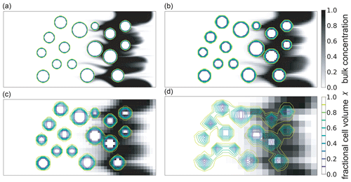
Figure 5 Results of the advection test with obstacles. Map plots of the concentration field of a test tracer after a simulation time of 150 s. The obstacles are drawn by contours of the volume-scaling field χ. Shown are the results of the flow simulations for the grids (a) 200×100 cells, (b) 100×50 cells, (c) 50×25 cells, and 25×13 cells, respectively.

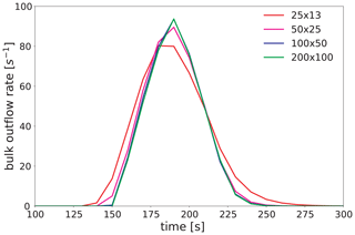
Figure 6 Washout curves of the test tracer for the different grid resolutions in Fig. 5. The values are computed by integrating over the modeled outflow at the downwind (right) domain border.

3.1 Advection through an obstacle field

In this 2-D test, the computation domain contains randomly positioned circular obstacles of varying size. In a first step, an approximate potential flow solution is computed. Therefore, one step of the pressure projection method is applied on the initial wind field defined by u=1 and v=0. The resulting potential flow field is used to advect a test-tracer front, which is solely characterized by the left inflow boundary condition:

$$\begin{array}{}\text{(47)}& c=\left\{\begin{array}{ll}\mathrm{1}& t\le \mathrm{40}\mathrm{s}\\ \mathrm{0}& t>\mathrm{40}\mathrm{s}.\end{array}\right.\end{array}$$

For the transversal-flow direction, periodic boundary conditions are used.

The reference simulation is carried out on a domain with 200×100 grid cells and a uniform grid spacing of 1 m. The obstacle radii range from 5 to 10 m. The simulation is repeated on coarser grids with dimension sizes of 100×50, 50×25, and 25×13, respectively. Figure 5 shows the simulation results at t=150 s. The obstacles are well resolved on the grid with 1 m spacing but become more and more diffuse with decreasing grid resolution towards 8 m for the coarsest grid. The initially planar test-tracer wave is delayed and deformed by the obstacles. The qualitative impression is that the shape of the wave is not very sensitive to the grid resolution. Even in the most diffuse case, the position and shape of the wave match that of the higher-resolved simulations well. The wave dispersion can be quantified by considering the washout curves shown in Fig. 6, which are the spatially averaged concentrations at the outflow boundary vs. time. For the case with the finest grid, the concentrations at the outflow boundary start to rise after t=145 s and peak at about t=185 s. At t=250 s, most of the wave is advected out of the domain. Remarkably, as already found by Calhoun and LeVeque (2000), the washout curve is not sensitive to the grid resolution up to 4 m, which is at the transition when obstacles start to become diffuse. For the case with the coarsest resolution of 8 m, the peak is slightly broader, peak concentrations are lower, and the peak occurs earlier by about 5 s. At this grid resolution, the numerical diffusion of the advection scheme becomes important, as the resolution capability is around six grid points, which is barely enough to resolve the wave.

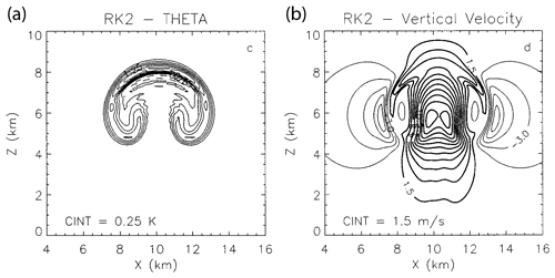
Figure 7 Original plot of Wicker and Skamarock (1998) (Fig. 5c–d therein) © American Meteorological Society. Used with permission. It shows the rising thermal problem computed using a third-order upwind scheme and a second-order Runge–Kutta scheme (Fig. 5c–d therein): shown are the potential temperature (a) and vertical velocity (b) after 1000 s of integration time.

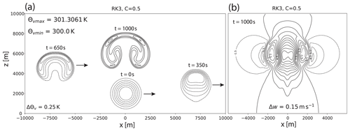
Figure 8 Rising thermal simulation with lateral advection: (a) contours of virtual potential temperature at different time steps. The initial and intermediate states are drawn with dashed lines; the final state at t=1000 s is drawn with solid lines. The contours with θ_v=300 K are omitted. (b) Contours of vertical wind speed at t=1000 s. Dashed lines are used for negative values.

3.2 Rising thermal

In the rising thermal simulation described in Wicker and Skamarock (1998), the Euler equations without diffusion are solved on a 2-D domain with a height of 10 km and a width of 20 km. The grid spacing is uniformly 125 m. The initially constant virtual potential temperature field of Θ_v=300 K is perturbed by a circular thermal:

$$\begin{array}{ll}{\displaystyle }\mathrm{\Delta }{\mathrm{\Theta }}_{\mathrm{v}}& {\displaystyle }=\left\{\begin{array}{ll}\mathrm{2}{\cos }^{\mathrm{2}}\left(\frac{\mathit{\pi }r}{\mathrm{2}L}\right)& r\le L\\ \mathrm{0}& r>L,\end{array}\right.\\ \text{(48)}& {\displaystyle }r& {\displaystyle }=\sqrt{x^{\mathrm{2}}+(z-\mathrm{2}\mathrm{km}{)}^{\mathrm{2}}},{\displaystyle }L& {\displaystyle }=\mathrm{2}\mathrm{km}.\end{array}$$

The initial vertical velocity is set to $w=\mathrm{0}\mathrm{m}{\mathrm{s}}^{-\mathrm{1}}$ and the horizontal velocity to $u=\mathrm{20}\mathrm{m}{\mathrm{s}}^{-\mathrm{1}}$. Periodic lateral boundary conditions are used and a rigid boundary is placed at the domain top. Due to buoyant forces, the thermal starts rising while it is constantly advected to the right and eventually re-enters the domain at the left boundary. After a simulation time of t=1000 s, the thermal is again situated in the center of the domain.

Figure 8a shows the evolution of the thermal based on contours of Θ_v at the time steps of t=0, t=350, t=650, and t=1000 s. Two distinct and symmetric rotors develop. At the simulation time of t=1000 s, the overall appearance of the thermal matches well that of the original simulation by Wicker and Skamarock (1998) as can be seen from the comparison with the original plot in Fig. 7. In our simulation, however, the thermal is more compact as it is confined between $x=\pm \mathrm{2300}$ m and the peak height is at about 8100 m. In the original simulation, it is confined between about $x=\pm \mathrm{2600}$ m and below 8500 m. Whether this slight discrepancy stems from the Boussinesq approximation or the different numerical schemes used can not be finally clarified. By scale analysis, the magnitude of the buoyant acceleration is about 1 or 2 orders less than that of the inertial acceleration in the given example. So, the Boussinesq approximation should indeed apply well in this example. The used fifth-order upwind scheme is much less diffusive than the third-order scheme used by Wicker and Skamarock (1998). On the other hand, the flux limiter introduces an adequate amount of diffusion near sharp gradients to prevent oscillations and to ensure a positive solution (θ_v≥300 K). This can explain our smoother contour lines inside the rotor. A slight asymmetry from the lateral advection can be noticed, which is most evident in the contours of vertical wind speed in Fig. 8b. This asymmetry can be slightly more reduced by decreasing the integration step size (not shown). The combination of the advection scheme with the third-order SSP-RK3 time scheme gives stable results up to a Courant number of C=0.7. Positivity of the solution is preserved up to C=0.5.

3.3 Strong scalability test

We tested parallel scalability of the model for a domain spanning 350×350 grid cells in the horizontal dimensions and 82 grid cells in the vertical, thus consisting of approximately 10 million cells in total. For realistic demands on the pressure solver, a grid of diffuse buildings was placed at the bottom of the domain and vertical grid stretching was applied. The high-performance computing platform we used for the scaling test is organized into nodes, each one equipped with two 12-core Intel Xeon E5-2680 v3 CPUs, making in total 24 cores per node available. The strong scalability test is carried out for a variable number of cores ranging from 1 to 400. The 400 cores correspond to a minimum average horizontal subdomain size of 17.5 grid cells. Figure 9 demonstrates the scaling efficiency of the model, as well as of the individual tasks for pressure projection and advection computation of three momentum components and two scalars, which together are responsible for the bulk of the computation time. As a reference, the dashed lines show ideal scaling starting from a reference of a single core. Comparing the experimentally obtained curves with the idealized curves, firstly, a peculiar drop in scaling efficiency between four and nine cores can be noticed. However, this drop cannot be explained by the parallelization design and it was also not observed using a different platform with less cores (not shown). The arithmetic-intense advection computation shows, apart from the already noted drop between four and nine cores, excellent scaling, which becomes even super-linear above 100 cores due to cache effects. Not surprisingly, the pressure solver, which requires two communications for each smoothing iteration, does not scale so well. While cache effects can balance the increasing communication overhead up to 200 cores, above this number, scaling is no longer satisfactory. Due to the lower costs of the pressure solution in comparison with the advection computation, the model shows a very good scaling up to 400 cores for this test case. Note, however, that the best decomposition to benefit from cache effects shifts toward a lower number of cores when the vertical dimension size is decreased. In theory, the implementation of the smoothing procedure supports overlapped communication and computation, as the matrix–vector product of the halo layer is computed independently from the inner matrix–vector product. In this test, we could not observe any true overlap, which would require further investigation. Addressing this feature in future can help to additionally improve scalability of the pressure solver.

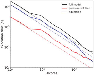
Figure 9 Strong scalability of CAIRDIO v1.0 tested for a domain with $\mathrm{350}\times \mathrm{350}\times \mathrm{82}$ grid cells using 1 to 400 cores on a high-performance computing platform. Dashed lines show ideal scaling.

Figure 10 (a) Depiction of the model domain for the numerical simulation of the “Michelstadt” wind-tunnel experiment. Rigid boundaries, including the buildings, the side walls, and the roughness elements are drawn using gray color. The yellow circles mark the tracer-gas release points. The dotted red line is at the position of the turbulence recycling plane. The area within the red bounding box contains the horizontal wind measurements arranged in horizontal planes. (b) Comparison of measured (black arrows) and modeled (red arrows) time-averaged horizontal wind vectors at 2 m height.

4 Model evaluation with wind-tunnel experiment and grid size sensitivity tests

The“Michelstadt” wind-tunnel experiment, which was carried out in the WOTAN wind tunnel (Lee et al., 2009) of the University of Hamburg, Germany, is used to evaluate the model accuracy and reliability of dispersion simulations within an urban canopy. Advantages of wind-tunnel data over field observations for model evaluation are the accurately controlled approaching-flow conditions and the high density of wind and concentration measurements in both space and time, which results in a high statistical significance of data (Schatzmann et al., 2017). The fictitious city district “Michelstadt” is based on a typical central European downtown area with spacious polygonal courtyards surrounded by residential building units at a scale of 1:225 (see Fig. 10a). Building roofs are approximated by horizontal surfaces, and their heights range from 15 to 25 m at the full scale. The approaching flow can be characterized by a neutrally stratified and horizontally homogeneous urban boundary layer with a parametric surface-roughness length of approximately 1.4 m. Experiments were carried out using two different approach-flow directions of 0 and 180^∘. This provides the opportunity to test the robustness of model results after model-parameter tuning using the wind-tunnel results from the default 0^∘ direction. The experimental dataset consists of time-resolved flow and dispersion measurements, from which temporally averaged statistics were calculated. A dense array of sensors provided horizontal wind measurements within planes at heights of 2, 9, 18, 27, and 30 m over a restricted area. For the dispersion modeling, neutrally buoyant gas was continuously released at different locations on the floor (see Fig. 10 for the locations of the release points). Release points S2 and S4 were used for the approach-flow direction of 0^∘, S6, S7, and S8 for the reverse direction. S5 was used for both wind directions. Tracer-gas detectors to measure concentrations were all positioned at a full-scale height of 7.5 m and at different horizontal positions depending on the source. Further information on the experiment and the datasets is provided in Baumann-Stanzer et al. (2015). The numerical simulations are performed at the full scale using a series of grids with horizontal resolutions of 5, 10, 20, 40, and 80 m. The 5 m horizontal resolution is used as the reference. The coarser domains are used to test the grid sensitivity of the dispersion simulation. The vertical grid spacing near the surface ranges from 2 m for the finest grid to 7 m for the coarsest ones. It is increasingly stretched beyond 30 m above surface. The effective domain height is approximately 600 m, which corresponds to the scaled wind-tunnel height. Above this height, the wind components are dampened to the horizontally and temporally average state. A first precursor simulation is run with periodic boundary conditions to obtain laminar and turbulent inflow profiles for the full vertical domain extent. These are used to drive the actual experimental simulations containing the buildings and test-tracer release points. In the precursor simulation, which uses a shorter domain with a total length of roughly 1 km, buildings are not present and the entire rigid bottom-domain boundary is covered with roughness elements. The geometries and arrangement of elements are adapted from the experiment. In order to model the effect of the lateral wind-tunnel confinement, rigid walls are placed at the flow-perpendicular boundaries. The modeled statistics of the established neutrally stratified boundary-layer flow are rescaled to the reference wind speed of 6 m s⁻¹ at 50 m height. The obtained horizontally averaged vertical profiles are vertically interpolated for the coarse-grid simulations. In the experimental simulations containing the model city, turbulent approach-flow conditions with the correct target intensities are generated using the turbulence-recycling scheme. The recycling plane is placed well downstream of the model city and after a short pattern of roughness elements near the outflow boundary (Fig. 10a). This allows for a much shorter additional domain fetch necessary for turbulence generation. This particular positioning of the recycling plane is also well supported by the similar parametric roughness length of the elements and the model city. Also, the extracted fluctuation intensities are rescaled to the values of the target wind field, which further reduces the impact of obstacles further upstream.

Figure 11 Modeled (dotted lines) and measured (full lines) mean and turbulent statistics of the approach flow in the “Michelstadt” wind-tunnel experiment. Depicted are (a) the temporal mean velocity component $\stackrel{\mathrm{‾}}{u}$ and (b–d) the grid-scale turbulent intensities $\stackrel{\mathrm{‾}}{u^{\prime }}$, $\stackrel{\mathrm{‾}}{v^{\prime }}$, and $\stackrel{\mathrm{‾}}{w^{\prime }}$, respectively.

4.1 Inflow profile

Figure 11 shows the modeled and rescaled horizontally averaged statistics of the boundary-layer flow generated by the precursor simulation. The experimentally obtained profiles are included for comparison. In the modeled mean horizontal wind speed, the roughness layer extends up to 20 m height, above which it is proceeded by the logarithmic Prandtl layer. The slope of the modeled wind profile in the semi-logarithmic depiction matches the observed profile well. The modeled turbulent intensities are generally underestimated by up to 20  % when compared with the observations. This difference is most likely due to artificial dissipation in the model. The peak values at about 400 m height are probably residual reflections at the domain top, which are not completely prevented by the dampening. The measurements below a height of 20 m are more difficult to compare, since they are located within the roughness layer and thus are strongly influenced by the relative location to the nearby roughness elements.

Figure 12 Scatter plot of modeled vs. measured horizontal wind speed within planes at different heights. For a quantitative comparison, NMSE and FB are calculated.

4.2 Horizontal wind evaluation

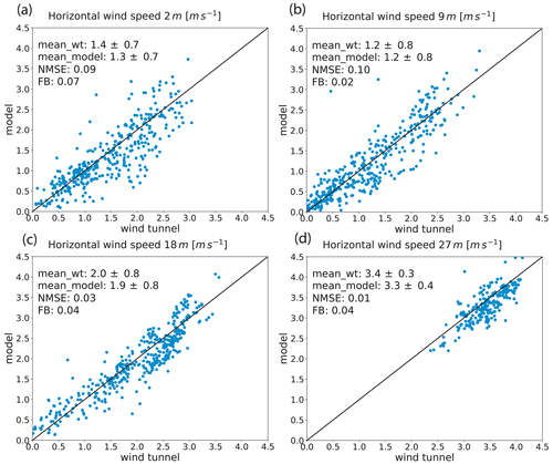
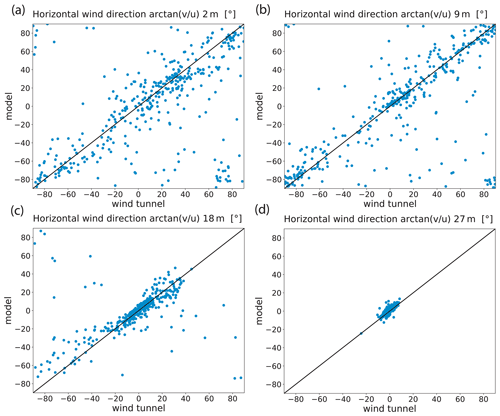
The modeled horizontal wind is evaluated on the reference grid with 5 m horizontal resolution. Figure 10b gives a first qualitative impression of the agreement. It shows the time-averaged horizontal wind vectors both for the model and the measurements within the plane of 2 m height. Overall, the model is capable of reproducing the measured flow pattern. However, the modeled wind direction does not always match the corresponding measured vector well, which is most notable near some intersections. The scatter plots for wind speed (Fig. 12) and wind direction (Fig. 13) give a more quantitative and conclusive picture. The accuracy of modeled wind speed is high taking the normalized mean standard error (NMSE) as a proxy. Its value is consistently below 0.1. The fractional bias (FB) shows only a very slight underestimation of the wind speed (0.02–0.07). This is not very surprising, as the model resolution of 5 m is not high enough to completely resolve the recirculation zones within the urban canopy (Xie and Castro, 2006). Thus, the modeled wind speed within circulation zones tends to be lower as a result of more extensive spatial averaging.

Figure 13 Scatter plot of modeled vs. measured horizontal wind direction within planes at different heights.

4.3 Dispersion evaluation

The resulting time-averaged modeled concentrations are interpolated to the detector sites and paired with corresponding measurements. As a proxy for the quality of model results in comparison to the measurements, NMSE, FB, and additionally the fraction of within a factor of 2 (FAC2) are calculated. Based on the guidelines presented in Hanna and Chang (2012), acceptance criteria for a valid simulation are NMSE<6, $\left|\mathrm{FB}\right|<\mathrm{0.67}$, and FAC2>0.3.

The simulations with the approach-flow direction of 0^∘ are used to optimize the model configuration with respect to these test criteria, while the reverse flow direction is used to validate the robustness of model results using the same parameter configuration. One important model tuning parameter is the Smagorinsky constant, which was set to c_s=0.15 for all simulations. However, for the simulations with 40 and 80 m resolution, the vertical mixing length had to be increased to 20 m within the urban canopy to compensate for the poorly defined eddies important for vertical mixing. Among the tested sources, S2 is the only one emitting into an open area, whereas all other sources are placed within street canyons or courtyards. Thus, S2 is probably the least difficult to simulate. Figure 14 gives an impression of the simulated time-averaged plumes resulting from S2 at the height of detector sites. Figure 14a shows the reference simulation with the highest grid resolution. The overall qualitative agreement with measurements seems very good, except for a street canyon in roughly −45^∘ direction and in close proximity to the source. Therein, the modeled concentrations are too low. Expectedly, increasing the grid spacing results in a deterioration of the qualitative agreement with measurements and with the reference simulation. For example, increasingly less tracer gas is advected inside the flow-parallel street canyon, where most of the detectors reside. Instead, the plumes are increasingly smeared over a wider area. This is especially evident for the 20 m grid spacing, whereas for the even coarser resolutions of 40 m, the agreement with measurements improves again. Notably, this behavior is only observed for this particular source. The grid resolution of 80 m clearly shows the least accurate results. While the dispersion pattern still resembles those of the better resolved simulations and shows the imprint of buildings, concentrations are too high in the downwind swath. At this resolution, a more elaborate mixing parameterization could still give improved results over the simple Smagorinsky model.

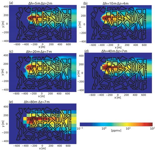
Figure 14 Map plots of modeled concentration fields in ppmv at 7.5 m height for source S2 and different grid resolutions. The black circles mark the location of measurements for this particular source, and the fill color indicates the measured concentration according to the color bar of the map plots.

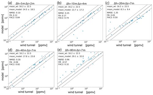
Figure 15 Scatter plots of measured vs. modeled concentrations for source S2 and different grid resolutions. The dotted lines confine the region within a factor of 2 of measurements.

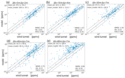
Figure 16 Scatter plots of measured vs. modeled concentrations combined for all sources and different grid resolutions. The dotted lines confine the region within a factor of 2 of measurements.

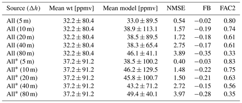
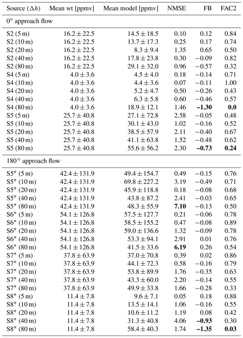
For the quantitative evaluation of the presented simulations, modeled and measured values are compared in scatter plots in Fig. 15, and the aforementioned statistical acceptance parameters are derived. For the reference case, most of the model data are tightly distributed near the bisecting line. In fact, the model accuracy is very good (NMSE=0.10), with only a slight positive bias toward too-low values (FB=0.12) and only few outliers present (FAC2=0.84). The decrease in model accuracy with increasing grid spacing is evident in the scatter plots, as modeled values tend to be too low for high concentrations measured, and vice versa. This results in a steady increase in NMSE=0.25 for the 10 m grid spacing and NMSE=1.35 for the 20 m grid spacing. Since FB is more sensitive to deviations at the upper end of the logarithmic scale, the smearing also results in an increasingly positive bias (FB=0.17 and FB=0.65). The trend is, however, reversed at the even coarser resolution of 40 m, resulting in an improvement of model results for this particular source. Finally, the 80 m case shows a large negative bias ($\mathrm{FB}=-\mathrm{0.57}$) and a value of FAC2=0.32 at the verge of acceptance. Table A1 summarizes the statistical parameters for all other simulated cases. From the sensitivity results in Table A1, it can be concluded that the quality of model results generally declines with decreased grid resolution (mostly evident in NMSE value) but not to an extent to compromise model reliability at up to 40 m resolution, where buildings are only represented diffusely. Only one source located within a courtyard was problematic to model with 40 m grid spacing, as the resulting plume was not well contained within. We attributed this to the difficulty in representing diagonally oriented building walls as impermeable as they are at such coarse resolutions. Using the 80 m grid, the model still performs acceptably for some of the sources. Figure 16 shows scatter plots of modeled and observed data collected from all simulated cases with a given resolution. The according statistical results are again summarized in Table A2. It is shown that the reliability of model results is not very sensitive to the grid spacing down to 40 m resolution. For example, FAC2 decreases from a value of 0.8 at 5 m to 0.61 at 40 m grid spacing. Conversely, NMSE increases from 0.54 to 2.75, which is still well within the acceptable range. The average fractional bias is below FB=0.2 for all simulations, except for the 80 m case, where it is much larger ($\mathrm{FB}=-\mathrm{0.35}$). In this regard, the increased vertical mixing length showed to be an effective tuning option in combination with the 40 m resolution to keep the bias comparatively low ($\mathrm{FB}=-\mathrm{0.17}$). It has to be kept in mind that this test uses isolated point sources. When applied to a more realistic scenario with traffic emissions, modeled, for example, by emission lines, it can be hypothesized that scattering of the data would be of less a concern, because the pollution is more widely distributed horizontally. Therefore, ultimately, the most important reliability measure in our view is the FB value, as it is a proxy of whether the model will under- or overestimate air pollution. In this regard, the 80 m resolution is the least accurate, and it is currently not reached without the use of a more sophisticated mixing parameterization. Finally, when comparing all model results with only those from the 180^∘ approach-flow tests using the same parameter configuration, it was found that these latter cases could be modeled not significantly less accurately. This is largely attributed to the simplicity of the model, as it requires little parameter tuning.

5 Summary

In this paper, the new large-eddy-simulation-based CAIRDIO model for urban dispersion simulations was presented. The model uses diffuse obstacle boundaries in the framework of a finite volume discretization to represent building walls at a wide range of spatial resolutions. Diffuse obstacle boundaries allow for a consistent implementation of buildings in the model code, as they are essentially described by a scalar field for the volume-scaling factors and a vector field for the area-scaling factors. Using these fields to discretize the differential operators, boundary conditions are incorporated automatically and the governing equations are solved for the entire computation grid without the need to distinguish different types of grid cells. This allows for a straightforward and vectorized implementation of spatial operations. The inherent option for under-resolved diffuse buildings enables the model to be applied at marginal grid resolutions inaccessible for conventional Cartesian grid models. The computational savings can be invested in larger domains to model whole city areas and its surroundings. The large-scale influence of orographic terrain can be adequately represented by curvilinear grids. To benefit from modern hardware architecture, the model is parallelized using a 2-D domain decomposition method, which is sufficient for the expected large grid-aspect ratios of typical boundary-layer applications. The numerical schemes presented are approved and efficient choices. Linear upwind schemes of selectable order of accuracy with optional limiting are used for advection, a static Smagorinsky model for subgrid turbulence modeling, and multi-stage higher-order time methods for model integration. The coupling with the mesoscale meteorology can be obtained through different forcing methods by using data from a mesoscale host model. A simple numerical test, consisting of a test tracer being advected by a potential flow through an obstacle field, demonstrated the robustness of the obstacle discretization up to grid spacings where the resolution capability of the numerical schemes starts to interfere. The results of the rising thermal experiment to test the dynamic core are plausible and similar to those presented in the original studies. Finally, we evaluated the model with data from the “Michelstadt” wind-tunnel experiment. In this study, the model reproduced reliably the complex wind fields and embedded tracer dispersion. For the latter application, this was also true using spatial resolutions beyond 20 m, at which buildings can only be represented as increasingly diffuse features. The sensitivity study researching grid spacing of the dispersion test showed promising results for a future study with more realistic emission distributions and real-sized cities. In the near future, also the coupling with mesoscale meteorology will be addressed. From previous and accompanying air-quality studies, simulations with the regional COSMO-MUSCAT CTM are available for different German cities, including Berlin and Leipzig, for which also comprehensive measurement data are available for model evaluation. In this framework, a promising application could be a more comprehensive and holistic model evaluation with field data, as mobile measurements are available for the city of Leipzig in addition to operational air monitoring. Potential model improvements worthy of being addressed in the future are the parameterization of air pollution sinks and the implementation of a simple urban atmospheric chemistry. Alternatively, it would be interesting to include diffuse obstacle boundaries in the MUSCAT aerosol–chemistry code and to investigate whether there is a benefit for the application on urban-air-pollution modeling.

Appendix A

Table A1 Statistical results of all dispersion simulations performed in the “Michelstadt” wind-tunnel simulation study. The cases superscripted with an asterisk were carried out using the reverse approach-flow direction of 180^∘. Missed acceptance criteria are highlighted in bold font.

Table A2 Statistical results derived from the combined data of all simulated sources at the given spatial resolution. The cases superscripted with an asterisk are the combined results of the 180^∘ approach-flow cases only.