PLUME-MoM-TSM 1.0.0: a volcanic column and umbrella cloud spreading model

In this paper, we present a new version of PLUME-MoM, a 1-D integral volcanic plume model based on the method of moments for the description of the polydispersity in solid particles. The model describes the steady-state dynamics of a plume in a 3-D coordinate system, and a modification of the two-size moment (TSM) method is adopted to describe changes in grain size distribution along the plume, associated with particle loss from plume margins and with particle aggregation. For this reason, the new version is named PLUME-MoM-TSM. For the first time in a plume model, the full Smoluchowski coagulation equation is solved, allowing us to quantify the formation of aggregates during the rise of the plume. In addition, PLUME-MOM-TSM allows us to model the phase change of water, which can be either magmatic, added at the vent as liquid from external sources, or incorporated through ingestion of moist atmospheric air. Finally, the code includes the possibility to simulate the initial spreading of the umbrella cloud intruding from the volcanic column into the atmosphere. A transient shallow-water system of equations models the intrusive gravity current, allowing computation of the upwind spreading.

The new model is applied first to the eruption of the Calbuco volcano in southern Chile in April 2015 and then to a sensitivity analysis of the upwind spreading of the umbrella cloud to mass flow rate and meteorological conditions (wind speed and humidity). This analysis provides an analytical relationship between the upwind spreading and some observable characteristic of the volcanic column (height of the neutral buoyancy level and plume bending), which can be used to better link plume models and volcanic-ash transport and dispersion models.

1 Introduction

In the last years, the simulation of ash dispersal in the atmosphere has become an ordinary activity for volcanic observatories and meteorological offices. Volcanic ash represents one of the major hazards associated with explosive eruptions, affecting both the proximity of the volcanic vent, where it can damage vegetation and infrastructures, and pose a health risk to people, and the surrounding atmosphere, requiring effective and prompt actions to regulate flights near the ash plume (Bonadonna et al., 2021).

In order to properly model the transport of ash and its associated deposition on the ground, it is important to provide the correct inputs to volcanic-ash transport and dispersion (VATD) models, and so far the best approach has been to use the output of numerical models simulating the rise of volcanic columns up to the neutral buoyancy level, where ash clouds transported by the wind spread in the atmosphere. Column models can be broadly categorized in two classes: one-dimensional (1-D) integral models (Bursik, 2001; Mastin, 2007; Degruyter and Bonadonna, 2012; Devenish, 2013; Woodhouse et al., 2013; de' Michieli Vitturi et al., 2015; Folch et al., 2016) and three-dimensional (3-D) models (Oberhuber et al., 1998; Suzuki and Koyaguchi, 2009; Cerminara et al., 2016; Ongaro et al., 2007). A recent intercomparison exercise (Costa et al., 2016) has shown that 1-D and 3-D models, notwithstanding that the formulations are different, produce consistent predictions of some of the more relevant quantities describing volcanic plumes, as, for example, the neutral buoyancy level. For this reason, in operative contexts where multiple scenarios have to be considered and the simulation time is an important constraint, 1-D models are still preferred. This class of models is based on the theory of turbulent buoyant plumes, as introduced by Morton et al. (1956), and it has been first applied in the volcanic context by Sparks (1986) and Woods (1988), who modeled the rising plume as a homogeneous mixture of gas and ash particles. Later works incorporated additional processes, such as the effects of moisture (Woods, 1993; Mastin, 2007) and ambient wind (Bursik, 2001).

Despite the relatively high number of integral models developed in the past couple of decades, some important features of volcanic plumes have been neglected so far, or they have not been considered together in a single model. Most notably, only a few models account for the thermodynamic phase relations for water (Herzog et al., 1998). As pointed out in several works (Koyaguchi and Woods, 1996; Woods, 1993; Sparks et al., 1997; Mastin, 2007), the presence of water, coming both from entrainment during some Surtseyan eruptions (Þórarinsson, 1967) or from entrainment of water-saturated air (Graf et al., 1999), and the thermodynamics of condensation and evaporation, can strongly affect the rise and collapse of strong volcanic plumes. Conversely, in Woodhouse et al. (2013), it is shown that for small weak plumes, the effect on height of external humidity entrained in the eruption column is almost negligible when compared to the role played by the uncertainty in parameters like source buoyancy flux, atmospheric stratification, and wind.

Another process that is frequently disregarded in the modeling of volcanic plumes is solid particle aggregation (Brown et al., 2012). So far, the number of works quantitatively describing aggregation processes in an eruption column is limited (Veitch and Woods, 2001; Textor et al., 2006b, a; Brown et al., 2012; Folch et al., 2016; Künzli et al., 2018; Rossi et al., 2018). This is because this process is quite complex, from both physical and modeling perspectives, requiring a careful treatment of the evolving grain size distribution. In fact, aggregation leads to the formation, from fine ash, of coarser particles, resulting in larger settling velocities than the primary particles and thus with an increased fallout of fine ash from the plume margins. A proper treatment of aggregation is thus important to predict the effective grain size distribution of solid particles reaching the neutral buoyancy level and then advected by the wind into the atmosphere.

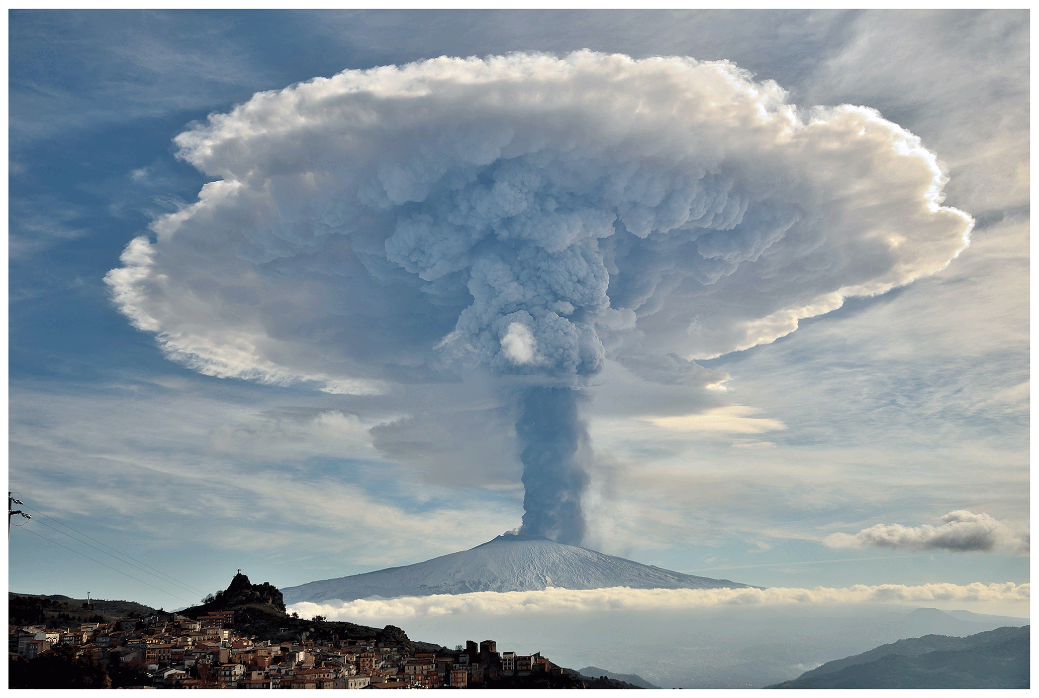
Figure 1 The 4 December 2015 paroxysm plume from Voragine crater at Mt. Etna, as viewed from Cesarò (Messina) at 09:27 GMT. Photo by Giuseppe Famiani. The volcanic column rose vertically and then spread horizontally at the neutral buoyancy level in all the directions.

For sustained eruptions, when neutral buoyancy level is reached, the eruptive mixture still has a vertical momentum, allowing the column to further rise and then to collapse as a gravity current spreading into the atmosphere (see Fig. 1). During the eruption of Mount St. Helens on 18 May 1980, this phenomenon was clear, and satellite data were used by Sparks (1986) to validate a simple model of umbrella spreading based on continuity of mass flow rate. For large mass eruption rates, this spreading can lead to an important radial expansion, including upwind transport, which is sometimes omitted in numerical simulations making use of coupled column and VATD models. In Costa et al. (2013), an analytical model describing the spreading of the umbrella cloud as a gravity current was coupled with an advection–diffusion–sedimentation model, and the conditions under which gravity-driven transport were analyzed. Baines (2013) studied the dynamics of this gravitational spreading into a density-stratified crossflow, deriving a semi-analytic model able to produce a good description of the behavior of the ash cloud in the proximity of intrusion from the column. A different approach to model the spreading of the umbrella cloud is presented in Johnson et al. (2015) where, following the work of Ungarish and Huppert (2002), the flow is modeled as a transient shallow-layer gravity current subject to gravitational forces and drag between the current and the surrounding atmosphere. The results of Johnson et al. (2015) show that the current spreads in a different way from what was suggested by simple scaling arguments in previous works, such as that of Costa et al. (2013). The same approach is used in Pouget et al. (2013, 2016), where the results of a “shallow-water” model are compared with satellite observations in order to estimate growth rates and mass fluxes. More recently, Folch et al. (2016) adopted a simple semi-empirical model to describe the umbrella region, and their results are qualitatively consistent with the results obtained with more complex 3-D numerical codes (Costa et al., 2016). A simple approach is also presented in Webster et al. (2020), where a parameterization is used to model the lateral spread of the umbrella and to correct the initial conditions for transport and dispersion in the Lagrangian model NAME, resulting in substantial improvements to ash cloud predictions for large explosive eruptions.

In this work, we extend the original PLUME-MoM model, which is the first volcanic plume model based on the method of moments for the description of the polydispersity in solid particles, by adding all the important features described above: phase transition of water, particle aggregation, and umbrella cloud spreading. The model is first applied to the April 2015 Calbuco eruption in Sect. 3.1, by comparing simulation results with observations to constrain some model parameters. Then, in Sect. 3.2, a sensitivity analysis is performed with the newly developed model in order to obtain a relationship first between eruption parameters and the upwind spreading of the umbrella cloud first, and then between the latter and other parameters characterizing the plume.

2 Model equations

In this section, we present the equations solved by PLUME-MoM-TSM. First of all, the new formulation for the description of the particle size distribution, based on the method of moments, is presented in Sect. 2.1. Then, in Sect. 2.2, the steady transport equations for the plume are derived from conservation principles (mass, momentum, and energy). The equations for the phase transition of water and the shallow-water equations describing the spreading of the umbrella cloud are finally presented in Sect. 2.3 and 2.4, respectively.

2.1 Solid particle number density function

As previously stated, particle aggregation is a complex process and its modeling requires an accurate description of the particle size distribution within a column and of its changes during the rise of the volcanic mixture. While particle fallout from the plume margin changes the size distribution but does not modify the size spectrum, aggregation leads to the formation of coarser particles, whose size was not present in the initial size distribution erupted at the vent. Furthermore, when a discretization in bins is employed to describe the variability in size, computational problems arise in the modeling of aggregation processes, because particles belonging to two bins of the original distribution could form an aggregate whose size is not represented in the chosen discretization. In this work, we try to solve these problems in the description and modeling of polydispersity in size of solid particles by adopting the method of moments.

In the first version of PLUME-MoM (de' Michieli Vitturi et al., 2015), the quadrature method of moments (QMOM) was used to model the polydispersity of tephra. According to the QMOM (Marchisio et al., 2003; Marchisio and Fox, 2013; Colucci et al., 2017), the particle size distribution is approximated from the moments as a sum of Dirac delta functions, which is particularly convenient for evaluating the integrals appearing in the closure terms of the moments transport equations. When aggregation processes are considered, QMOM provides an effective alternative to the sectional (or “discrete”) method, where the size spectrum is partitioned in discrete bins. Its advantages are a limited number of variables and the dynamic calculation of the more representative sizes within the distribution. The main disadvantage is that, given the moments of a distribution, it is not possible to retrieve the amount of mass associated with a size interval. This represents a problem when the output of a plume model is used as input of a model for transport and deposition of ash in the atmosphere.

To cope with this problem, we describe here a hybrid method combining the advantages of the sectional and moment methods. With this hybrid approach, the size spectrum is still partitioned in sections (or bins), and then the transport equations for a limited number of moments for each section are solved. The number density function (NDF) is then represented by using a piecewise reconstruction, continuous on each section. Among these hybrid methods, in several engineering contexts, like spray modeling, the two-size moment (TSM) method has proven to produce good results for size reduction simulations (i.e., evaporation) and for coalescence, by using in each section a second-order accurate reconstruction of the NDF from the first two moments (Nguyen et al., 2016), leading also to a good representation of the NDF with a small number of sections. For this reason, TSM is a good candidate for the modeling of the aggregation processes occurring in the volcanic column. In this paper, we introduce a modified version of the TSM method presented in Nguyen et al. (2016). While in the original formulation the internal variable is the size (described by the volume or the radius) of the particles and in each section two moments of the size distribution are used to reconstruct the NDF with a linear function of the size (hence the name “two-size moment”), here the NDF is defined as a function of particle mass. This greatly simplifies the formulation when aggregation is considered: two particles of mass (M₁ and M₂, respectively) aggregate in a new particle of mass ($M=M_{\mathrm{1}}+M_{\mathrm{2}}$). In addition, while in Nguyen et al. (2016) for some section the support of the linear reconstruction (the subset of the section containing the elements which are not mapped to zero) can be smaller than the section width (which means that the existing particles size spectrum do not cover entirely the respective section), we switch here from a linear reconstruction to a power law in these sections, with zero value at one of the boundaries of the section. The advantages of this approach will be explained in detail in the following.

The starting point of the TSM method is the partition of the size spectrum into n sections (or bins). Here, given a maximum size ϕ₀ and a size increment Δϕ, we define a uniform partition ${\mathit{\varphi }}_i={\mathit{\varphi }}_{\mathrm{0}}+i\mathrm{\Delta }\mathit{\varphi },i=\mathrm{0},\mathrm{\dots },n_{\mathrm{s}}$, in the non-dimensional Krumbein ϕ scale:

$$\begin{array}{}\text{(1)}& \mathit{\varphi }=-{\log }_{\mathrm{2}}{\displaystyle \frac{\mathrm{1000}\cdot D}{D_{\mathrm{0}}}},\end{array}$$

where D is the diameter of the particle expressed in meters, and D₀ is a reference diameter, equal to 1 mm (to make the equation dimensionally consistent). Given the particles' density ρ=ρ(ϕ) and their sphericity, it is possible to associate to each size of the original partition ϕ_i the corresponding particle mass m_i and thus to obtain a partition of the particles' mass spectrum in n_s sections corresponding to the n_s bins in the Krumbein scale. In this way, the internal variable characterizing the variability of the particle population becomes the mass, and its variability can be characterized by the solid particles' number density function (NDF), here denoted by $\mathit{\eta }(m,x,t)$. This function, which is formally a mass distribution, represents the number of solid particles per unit volume of the gas–particle mixture in the infinitesimal mass interval $[m;m+\mathrm{d}m]$ at the location x in space and at time t (according to this definition, the number density function $\mathit{\eta }(m,x,t)$ has units L⁻³ M⁻¹). With this choice, when we integrate the number density function in a fixed control volume V and over a mass interval [m₁,m₂], we obtain the number of particles in V at time t with mass between m₁ and m₂.

We introduce the following notation for the jth moment of the number density function η:

$$\begin{array}{}\text{(2)}& m^{\left(j\right)}=\underset{\mathrm{0}}{\overset{+\mathrm{\infty }}{\int }}\mathit{\eta }(m,x,t)m^j\mathrm{d}m.\end{array}$$

We observe that in the notation of the moment on the left-hand side of the equation we dropped the explicit dependence from x and t. Also in the rest of the paper, for the sake of simplicity, we will use without ambiguity the notation without x and t to denote the moments, even when they vary in space and time.

One important property of the NDF that is adopted is that its moments correspond to quantities that have meaningful physical interpretations and are therefore, at least in principle, directly measurable in the field, as well as in experiments. For example, we observe that the moment of order 0, m⁽⁰⁾, represents the total number of solid particles per unit volume of the mixture, while the moment of order 1, m⁽¹⁾, represents the total mass of solid particles per unit volume of the gas–particle mixture, i.e., the bulk density of the solid particles, here denoted by ${\mathit{\rho }}_{\mathrm{p}}^B$. From a physical point of view, these moments are commonly the main variables of interest, since when there is no aggregation the global moment of order 0 is conserved, while with aggregation the global moment of order 1 is conserved. In addition, dividing the first moment by the average solid particle density, we obtain the volume fraction of particles with respect to the volume of the gas–particle mixture.

As previously stated, the mass spectrum is partitioned in n sections, and we can define the local moments of orders 0 and 1 on the kth section defined by the mass interval $[m_{k-\mathrm{1}},m_k]$:

$$\begin{array}{}\text{(3)}& \begin{array}{rl}{N}_k(x,t)& =\underset{m_{k-\mathrm{1}}}{\overset{m_k}{\int }}\mathit{\eta }(m,x,t)\mathrm{d}m,M_k(x,t)\\ & =\underset{m_{k-\mathrm{1}}}{\overset{m_k}{\int }}\mathit{\eta }(m,x,t)m\mathrm{d}m.\end{array}\end{array}$$

Also in this case, the local moments have an important physical interpretation. In fact, the local moments of order 1 M_k represent the mass within each mass section per unit volume of the mixture, and thus, when normalized, they give the total grain size distribution. Solving appropriate transport equation for the moments M_k allows one to describe the evolution of the total grain size distribution within the plume. We observe that, conversely to the global moment of order 1, the local moments of order 1 are not conserved by aggregation, because mass moves from sections corresponding to finer particles to sections corresponding to coarser ones.

The local moments of other quantities ψ(m) which depend on particle mass, as, for example, the density, or the settling velocity, can be defined in terms of the continuous number density function η(m) as

$$\begin{array}{}\text{(4)}& {\mathit{\psi }}_k^{\left(i\right)}={\displaystyle \frac{\mathrm{1}}{m^{\left(i\right)}}}\underset{m_{k-\mathrm{1}}}{\overset{m_k}{\int }}\mathit{\psi }\left(m\right)m^i\mathit{\eta }\left(m\right)\mathrm{d}m.\end{array}$$

This term has the same units of ψ(m) and represents its integral average, weighted differently according to the order of the moment. For example, ${\mathit{\psi }}_k^{\left(\mathrm{0}\right)}$ represents the average of ψ in the mass interval $[m_{k-\mathrm{1}},m_k]$ weighted by the number of solid particles, while ${\mathit{\psi }}_k^{\left(\mathrm{1}\right)}$ represents a mass-weighted average in the same interval.

When the moments of the number density function η are known for each section but not the actual expression of η, the integral in Eq. (4) must be approximated with a quadrature formula. To do this, we need the “weights” and the “nodes” (or “abscissae”) of the quadrature. Here, we use an approach based on the Gauss–Legendre quadrature, which can be written as

$$\begin{array}{}\text{(5)}& \underset{-\mathrm{1}}{\overset{\mathrm{1}}{\int }}f\left(x\right)\mathrm{d}x\approx \sum _{i=\mathrm{1}}^n{\mathit{\omega }}_{i}f\left(x_i\right),\end{array}$$

where the ith node x_i is the ith root of the Legendre polynomial P_n(x) and the weights ω_i are given by the Abramowitz–Stegun 1972 formula (Abramowitz and Stegun, 1965). This n-points quadrature formula is exact for polynomials of degree 2n−1 or less. From these quadrature nodes and weights defined for the standard interval $[-\mathrm{1},\mathrm{1}]$, it is possible to compute the nodes and weights for the integral over the interval $[m_{k-\mathrm{1}},m_k]$:

$$\begin{array}{}\text{(6)}& \underset{m_{k-\mathrm{1}}}{\overset{m_k}{\int }}f\left(x\right)\mathrm{d}x\approx \sum _{i=\mathrm{1}}^n{\stackrel{\mathrm{̃}}{\mathit{\omega }}}_{k,i}f\left({\stackrel{\mathrm{̃}}{x}}_{k,i}\right),\end{array}$$

where

$$\begin{array}{}\text{(7)}& \begin{array}{rl}& {\stackrel{\mathrm{̃}}{\mathit{\omega }}}_{k,i}={\displaystyle \frac{m_k-m_{k-\mathrm{1}}}{\mathrm{2}}}{\mathit{\omega }}_i\\ & {\stackrel{\mathrm{̃}}{x}}_{k,i}={\displaystyle \frac{m_k-m_{k-\mathrm{1}}}{\mathrm{2}}}{x}_i+{\displaystyle \frac{m_{k-\mathrm{1}}+m_k}{\mathrm{2}}}.\end{array}\end{array}$$

With this approach, when the integrand of Eq. (4) changes (for example, because the number density function, i.e., the mass distribution, changes in space or time), there is no need to re-evaluate the quadrature nodes and weights, which depend only on the interval and can be computed in advance. The only thing to update is the value of the integrand at the quadrature points. In the TSM approach, as presented in Nguyen et al. (2016), the number density function η(m) is approximated in each section by a linear function. Here, non-linear approximations $\approx {\stackrel{\mathrm{̃}}{\mathit{\eta }}}_k\left(m\right)$ of the number density function are considered. On each section k, a continuous reconstruction is assumed:

$$\begin{array}{}\text{(8)}& \mathit{\eta }\left(m\right){|}_{m\in [m_{k-\mathrm{1}},m_k]}={\mathit{\eta }}_k\left(m\right)\approx {\stackrel{\mathrm{̃}}{\mathit{\eta }}}_k\left(m\right),\end{array}$$

where three possible continuous reconstructions are used for each ${\stackrel{\mathrm{̃}}{\mathit{\eta }}}_k\left(m\right)$, as illustrated in Fig. 2:

$$\begin{array}{}\text{(9)}& \begin{array}{rl}& {\stackrel{\mathrm{̃}}{\mathit{\eta }}}_k\left(m\right)\\ & =\left\{\begin{array}{ll}\left[{\mathit{\beta }}_k{\left(\frac{m-m_{k-\mathrm{1}}}{m_k-m_{k-\mathrm{1}}}\right)}^{{\mathit{\gamma }}_k}\right]{\mathbf{1}}_{[m_{k-\mathrm{1}},m_k]}\left(m\right)& \mathrm{CASE}\mathrm{1}\\ & \\ \left[{\mathit{\alpha }}_k+({\mathit{\beta }}_k-{\mathit{\alpha }}_k)\frac{m-m_{k-\mathrm{1}}}{m_k-m_{k-\mathrm{1}}}\right]{\mathbf{1}}_{[m_{k-\mathrm{1}},m_k]}\left(m\right)& \mathrm{CASE}\mathrm{2}\\ & \\ \left[{\mathit{\alpha }}_k{\left(\frac{m_k-m}{m_k-m_{k-\mathrm{1}}}\right)}^{{\mathit{\gamma }}_k}\right]{\mathbf{1}}_{[m_{k-\mathrm{1}},m_k]}\left(m\right)& \mathrm{CASE}\mathrm{3}\end{array}\right.\end{array}\end{array}$$

The parameters α_k, β_k (representing the values of the reconstructed function at m_k−1 and m_k), and γ_k are computed in order to have

$$\begin{array}{}\text{(10)}& {\stackrel{\mathrm{̃}}{\mathit{\eta }}}^{\left(\mathrm{0}\right)}=N_k,{\stackrel{\mathrm{̃}}{\mathit{\eta }}}^{\left(\mathrm{1}\right)}=M_k.\end{array}$$

In this way, the domain of each function ${\stackrel{\mathrm{̃}}{\mathit{\eta }}}_k\left(m\right)$ is always the whole kth section, and there is no need to update the quadrature nodes. Further details on the selection of the case and the computation of the parameters α_k and β_k are given in Appendix A.

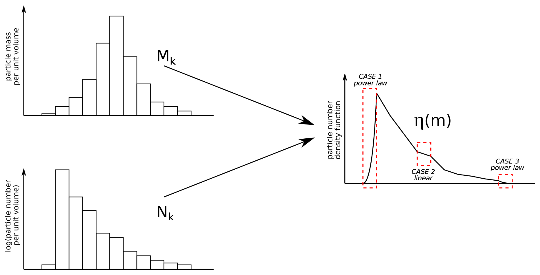
Figure 2 Piecewise reconstruction of the number density function from the local moments. The values of the first two moments in each section (plotted on the two bar plots on the left) are used for the reconstruction of the piecewise continuous density function. The function is linear in the internal sections and a power law at the boundaries.

So far, we presented the TSM approach for a single family of particles. When more than one particle family is considered (for example, if we consider aggregation and we want to distinguish between aggregated and non-aggregated particles), the subscript i_p is used to distinguish the different number density functions ${\mathit{\eta }}_{i_{\mathrm{p}}}\left(m\right),i_{\mathrm{p}}=\mathrm{1},\mathrm{\dots },n_{\mathrm{p}}$, where n_p is the number of particles families. Similarly, the notation $m_{i_{\mathrm{p}}}^{\left(j\right)}$ is introduced for the jth moment of the i_pth number density function, and the notations $N_{i_{\mathrm{p}},k}$ and $M_{i_{\mathrm{p}},k}$ for the number and mass of particles of the i_pth family in the kth section, respectively.

2.2 Plume equations

In this section, we present the set of conservation equations describing the steady rise (d $/$ dt=0) of the volcanic mixture through the atmosphere. The model we present, based on the buoyant plume theory of Morton et al. (1956), is a 1-D integral model where plume properties are averaged over cross-sections. As in Bursik (2001), the model assumes a homogeneous mixture of different phases with thermal and mechanical equilibrium among all of them. In this version of the model, in addition to air and solid particles, we also explicitly model the presence of water, which can be in gas, liquid, or solid state, and the presence of additional volcanic gases, such as CO₂ and SO₂ (transported as passive components). The equation set for the plume rise model is solved in a 3-D coordinate system (x, y, z) centered horizontally at the plume base location and vertically at the sea level. The plume is assumed with a circular section with radius r, parallel to the horizontal plane (x, y) and orthogonal to the vertical coordinate z (see Fig. 3).

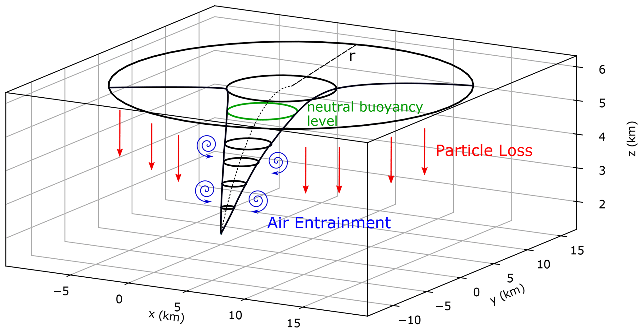
Figure 3 Schematic view of the plume. The dashed line represents the centerline of the plume. The horizontal circles indicate the sections over which plume variables are averaged. The green circle represents the plume section at the neutral boundary level.

In the (x, y, z) coordinate system, we denote u, v, and w as the three components of plume velocity, and $U_{\mathrm{sc}}=\sqrt{u^{\mathrm{2}}+v^{\mathrm{2}}+w^{\mathrm{2}}}$ its magnitude. Furthermore, we define ζ as the angle between the axial direction and the horizontal plane, for which the following relationship holds:

$$\tan \mathit{\zeta }={\displaystyle \frac{w}{\sqrt{u^{\mathrm{2}}+v^{\mathrm{2}}}}}.$$

We also consider the presence of a horizontal atmospheric wind, with velocity components u_a, v_a, and magnitude U_atm. Because of the wind, the location of the centers of the horizontal sections, which defines the plume centerline, can be bent, and the following equations hold for the centerline coordinates $x_s,y_s,z_s$:

$$\begin{array}{}\text{(11)}& {\displaystyle \frac{\mathrm{d}{x}_s}{\mathrm{d}z}}={\displaystyle \frac{u}{w}},{\displaystyle \frac{\mathrm{d}{y}_s}{\mathrm{d}z}}={\displaystyle \frac{v}{w}},{\displaystyle \frac{\mathrm{d}{z}_s}{\mathrm{d}z}}=w.\end{array}$$

When more than one particle family is considered, they are denoted by the subscript $i_{\mathrm{p}}=\mathrm{1},\mathrm{\dots },n_{\mathrm{p}}$; in addition, if aggregation is considered, we use the first n_p−1 indexes for the original particles and the last one for the aggregated particles. With this notation, for the particles with mass m of the family i_p, we can write the following equation for the vertical mass flux through a horizontal cross-section of the plume (see Fig. 3):

$$\begin{array}{}\text{(12)}& {\displaystyle \frac{\mathrm{d}}{\mathrm{d}z}}\left({\mathit{\eta }}_{i_{\mathrm{p}}}(m,z)\mathit{\pi }{r}^{\mathrm{2}}w\right)=-\mathrm{2}\mathit{\pi }rp{w}_{i_{\mathrm{p}}}\left(m\right)\cdot {\mathit{\eta }}_{i_{\mathrm{p}}}(m,z)+S_{i_{\mathrm{p}}},\end{array}$$

where both the plume radius r and the vertical component of the plume axial velocity w vary with the vertical coordinate z. Equation (12) describes the variation with the vertical coordinate z of the mass flux of particles of size m, due to fallout of tephra (first term on the right-hand side) and aggregation (second term on the right-hand side, $S_{i_{\mathrm{p}}}$). Here, $w_{i_{\mathrm{p}}}(\cdot )$ is the particle settling velocity (see Appendix B2) and the coefficient p, which is a function of the radial entrainment coefficient α, expresses the probability that an individual particle will fall out of the plume (Bursik et al., 1992):

$$\begin{array}{}\text{(13)}& p={\displaystyle \frac{{\left(\mathrm{1}+\frac{\mathrm{6}}{\mathrm{5}}\mathit{\alpha }\right)}^{\mathrm{2}}-\mathrm{1}}{{\left(\mathrm{1}+\frac{\mathrm{6}}{\mathrm{5}}\mathit{\alpha }\right)}^{\mathrm{2}}+\mathrm{1}}}.\end{array}$$

The last term on the right-hand side of Eq. (12) represents the aggregation term which, following Smoluchowski (1917), can be written as

$$\begin{array}{}\text{(14)}& {\displaystyle }\begin{array}{rl}& S_{i_{\mathrm{p}}}(m,z)=-\mathit{\pi }{r}^{\mathrm{2}}\sum _{l_{\mathrm{p}}=\mathrm{1}}^{n_{\mathrm{p}}}\left({\mathit{\eta }}_{i_{\mathrm{p}}}(m,z)\underset{\mathrm{0}}{\overset{+\mathrm{\infty }}{\int }}\mathit{\beta }(z,m,m^{\prime }){\mathit{\eta }}_{l_{\mathrm{p}}}(m^{\prime },z)\mathrm{d}{m}^{\prime }\right)\\ & i_{\mathrm{p}}=\mathrm{1},\mathrm{\dots },n_{\mathrm{p}}-\mathrm{1}\end{array}\text{(15)}& {\displaystyle }\begin{array}{rl}{S}_{n_{\mathrm{p}}}(m,z)& =\mathit{\pi }{r}^{\mathrm{2}}\sum _{l_{\mathrm{p}}=\mathrm{1}}^{n_{\mathrm{p}}}\left(\sum _{k_{\mathrm{p}}=\mathrm{1}}^{n_{\mathrm{p}}}{\displaystyle \frac{\mathrm{1}}{\mathrm{2}}}\underset{\mathrm{0}}{\overset{m}{\int }}\mathit{\beta }\right(z,m-m^{\prime },m^{\prime }){\mathit{\eta }}_{l_{\mathrm{p}}}\\ & (m-m^{\prime },z){\mathit{\eta }}_{k_{\mathrm{p}}}(m^{\prime },z)\mathrm{d}{m}^{\prime }\\ & -{\mathit{\eta }}_{n_{\mathrm{p}}}(m,z)\underset{\mathrm{0}}{\overset{+\mathrm{\infty }}{\int }}\mathit{\beta }(z,m,m^{\prime }){\mathit{\eta }}_{l_{\mathrm{p}}}(m^{\prime },z)\mathrm{d}{m}^{\prime }),\end{array}\end{array}$$

where $\mathit{\beta }(z,m,m^{\prime })$ is the aggregation (or coagulation) kernel describing the rate at which a particle of mass m aggregate with a particle of mass m^′. The equations state that the aggregation of particles of mass m and m^′, forming a particle of mass $m+m^{\prime }$, are proportional to the number density of particles of such masses (η(m) and η(m^′)) and to the aggregation kernel. The negative term on the right-hand side of the first equation represents the loss of solid particles of the original families due to aggregation. The positive term on the right-hand side of the second equation represents the increased number of particles of mass m at the vertical coordinate z due to aggregation of smaller particles. The aggregation kernel can be defined as the product of two quantities: the “collision frequency” between particles of mass m and m^′ and the “efficiency of aggregation” (i.e., the probability of particles of mass m coalescing with particles of mass m^′ when colliding). In PLUME-MoM-TSM, several aggregation kernels are implemented, from simple constant kernels to more complex formulations describing wet aggregation, where the collision frequency depends on particles properties (size, density) and the efficiency of aggregation depends on the amount of water in the mixture (see Appendix B3).

Let us consider now a mass interval Ω, which can be the whole solid particle mass spectrum or a smaller subset, as the kth section for the family i_p, defined by $[m_{i_{\mathrm{p}},k-\mathrm{1}},m_{i_{\mathrm{p}},k}]$. Multiplying Eq. (12) by mⁱ and integrating over Ω, we obtain the following differential equations for the moments:

$$\begin{array}{}\text{(16)}& {\displaystyle \frac{\mathrm{d}}{\mathrm{d}z}}\left(m_{i_{\mathrm{p}}}^{\left(i\right)}w{r}^{\mathrm{2}}\right)=-\mathrm{2}rp{w}_{i_{\mathrm{p}}}^{\left(i\right)}{m}_{i_{\mathrm{p}}}^{\left(i\right)}+{\widehat{S}}_{i_{\mathrm{p}}}^{\left(i\right)},\end{array}$$

where the last term is defined by

$$\begin{array}{}\text{(17)}& {\displaystyle }\begin{array}{rl}{\widehat{S}}_{i_{\mathrm{p}}}^{\left(i\right)}& =-\mathit{\pi }{r}^{\mathrm{2}}\sum _{l_{\mathrm{p}}=\mathrm{1}}^{n_{\mathrm{p}}}\left(\underset{\mathrm{\Omega }}{\int }{m}^i{\mathit{\eta }}_{i_{\mathrm{p}}}\right(m,z\left)\underset{\mathrm{0}}{\overset{+\mathrm{\infty }}{\int }}\mathit{\beta }\right(z,m,m^{\prime }){\mathit{\eta }}_{l_{\mathrm{p}}}\\ & (m^{\prime },z)\mathrm{d}{m}^{\prime }\mathrm{d}m)\\ & i_{\mathrm{p}}=\mathrm{1},\mathrm{\dots },n_{\mathrm{p}}-\mathrm{1}\end{array}\text{(18)}& {\displaystyle }\begin{array}{rl}{\widehat{S}}_{n_{\mathrm{p}}}^{\left(i\right)}& =\mathit{\pi }{r}^{\mathrm{2}}\sum _{l_{\mathrm{p}}=\mathrm{1}}^{n_{\mathrm{p}}}\left(\sum _{k_{\mathrm{p}}=\mathrm{1}}^{n_{\mathrm{p}}}{\displaystyle \frac{\mathrm{1}}{\mathrm{2}}}\underset{\stackrel{\mathrm{‾}}{\mathrm{\Omega }}}{\iint }\right(m+m^{\prime }{)}^i\mathit{\beta }(z,m,m^{\prime })\\ & {\mathit{\eta }}_{l_{\mathrm{p}}}(m,z){\mathit{\eta }}_{k_{\mathrm{p}}}(m^{\prime },z)\mathrm{d}m\mathrm{d}{m}^{\prime }\\ & -\underset{\mathrm{\Omega }}{\int }{m}^i{\mathit{\eta }}_{n_{\mathrm{p}}}(m,z)\underset{\mathrm{0}}{\overset{+\mathrm{\infty }}{\int }}\mathit{\beta }(z,m,m^{\prime }){\mathit{\eta }}_{l_{\mathrm{p}}}(m^{\prime },z)\mathrm{d}{m}^{\prime }\mathrm{d}m),\end{array}\end{array}$$

with $\stackrel{\mathrm{‾}}{\mathrm{\Omega }}=\left\{(m,m^{\prime })>\mathrm{0}\left|\right(m+m^{\prime })\in \mathrm{\Omega }\right\}$. The set $\stackrel{\mathrm{‾}}{\mathrm{\Omega }}$ represents the set of couples of particles which form, when aggregating, particles with mass in the interval Ω.

Let us consider now the kth section for the family i_p, defined by $[m_{i_{\mathrm{p}},k-\mathrm{1}},m_{i_{\mathrm{p}},k}]$. For i=0 and i=1, Eq. (16) gives the equations governing the evolution of the number of particles and mass of particles of the family i_p in the kth mass interval per unit volume of the mixture, respectively:

$$\begin{array}{}\text{(19)}& {\displaystyle \frac{\mathrm{d}}{\mathrm{d}z}}\left(N_{i_{\mathrm{p}},k}w{r}^{\mathrm{2}}\right)=-\mathrm{2}rp{w}_{i_{\mathrm{p}}}^{\left(\mathrm{0}\right)}{N}_{i_{\mathrm{p}},k}+{\widehat{S}}_{i_{\mathrm{p}},k}^{\left(\mathrm{0}\right)}\text{(20)}& {\displaystyle \frac{\mathrm{d}}{\mathrm{d}z}}\left(M_{i_{\mathrm{p}},k}w{r}^{\mathrm{2}}\right)=-\mathrm{2}rp{w}_{i_{\mathrm{p}}}^{\left(\mathrm{1}\right)}{M}_{i_{\mathrm{p}},k}+{\widehat{S}}_{i_{\mathrm{p}},k}^{\left(\mathrm{1}\right)}.\end{array}$$

We remark that so far we have written a general form of the moment equations, which are valid independently from the particular approach used to solve them (QMOM or TSM). As previously stated, when the TSM method is adopted, the integral terms on the right-hand side of the two previous equations ($w_{i_{\mathrm{p}}}^{(\cdot )}$ and ${\widehat{S}}_{i_{\mathrm{p}},k}^{(\cdot )}$) are calculated first by reconstructing the continuous number density functions in each section from the known moments (number and mass of solid particles in the kth section per unit volume of the mixture) and then approximating the integrals with the Gauss–Legendre quadrature formulas.

We also observe that when the equations for the mass of particles are added together (summed over the particles families and over the sections), the aggregation terms cancel out, and the following transport equation is obtained:

$$\begin{array}{}\text{(21)}& {\displaystyle \frac{\mathrm{d}}{\mathrm{d}z}}\left(\sum _{i_{\mathrm{p}}=\mathrm{1}}^{n_{\mathrm{p}}}\sum _{k=\mathrm{1}}^{n_{\mathrm{s}}}{M}_{i_{\mathrm{p}},k}w{r}^{\mathrm{2}}\right)=-\mathrm{2}rp\sum _{i_{\mathrm{p}}=\mathrm{1}}^{n_{\mathrm{p}}}\sum _{k=\mathrm{1}}^{n_{\mathrm{s}}}{w}_{i_{\mathrm{p}},k}^{\left(\mathrm{1}\right)}{M}_{i_{\mathrm{p}},k},\end{array}$$

which gives the total mass of solid particles per unit volume of the mixture lost because of particle sedimentation from the plume.

The right-hand side of the previous expression can be used in the mass conservation equation for the volcanic mixture accounting for air entrainment and particle sedimentation, which writes as

$$\begin{array}{}\text{(22)}& {\displaystyle \frac{\mathrm{d}}{\mathrm{d}z}}\left({\mathit{\rho }}_{\mathrm{mix}}w{r}^{\mathrm{2}}\right)=\mathrm{2}r{\mathit{\rho }}_{\mathrm{atm}}{U}_{\mathit{ϵ}}-\mathrm{2}rp\sum _{i_{\mathrm{p}}=\mathrm{1}}^{n_{\mathrm{p}}}\sum _{k=\mathrm{1}}^{n_{\mathrm{s}}}{w}_{i_{\mathrm{p}},k}^{\left(\mathrm{1}\right)}{M}_{i_{\mathrm{p}},k},\end{array}$$

where ρ_atm is the density of the atmosphere and U_ϵ is the entrainment velocity defined as in Hewett et al. (1971):

$$U_{\mathit{ϵ}}={\mathit{\alpha }}_{\mathit{ϵ}}|U_{\mathrm{sc}}-U_{\mathrm{atm}}\cos \mathit{\zeta }|+{\mathit{\gamma }}_{\mathit{ϵ}}\left|U_{\mathrm{atm}}\sin \mathit{\zeta }\right|.$$

In the previous equation, ${\mathit{\alpha }}_{\mathit{ϵ}}|U_{\mathrm{sc}}-U_{\mathrm{atm}}\cos \mathit{\zeta }|$ is entrainment by radial inflow minus the amount swept tangentially along the plume margin by the wind, and ${\mathit{\gamma }}_{\mathit{ϵ}}\left|U_{\mathrm{atm}}\sin \mathit{\zeta }\right|$ is entrainment from wind. Equation (22) states that the variation of mass flux along the plume axis (left-hand-side term) is due to ingestion of atmospheric air into the column (first right-hand-side term) and loss of particles from the column margins (second right-hand-side term).

The horizontal and vertical components of the momentum balance are derived from Newton's second law and the variation of mass flux as

$$\begin{array}{}\text{(23)}& {\displaystyle \frac{\mathrm{d}}{\mathrm{d}z}}\left({\mathit{\rho }}_{\mathrm{mix}}w{r}^{\mathrm{2}}u\right)=\mathrm{2}r{U}_{\mathit{ϵ}}{u}_e{\mathit{\rho }}_{\mathrm{atm}}-\mathrm{2}upr\sum _{i_{\mathrm{p}}=\mathrm{1}}^{n_{\mathrm{p}}}\sum _{k=\mathrm{1}}^{n_{\mathrm{s}}}{w}_{i_{\mathrm{p}},k}^{\left(\mathrm{1}\right)}{M}_{i_{\mathrm{p}},k},\text{(24)}& {\displaystyle \frac{\mathrm{d}}{\mathrm{d}z}}\left({\mathit{\rho }}_{\mathrm{mix}}w{r}^{\mathrm{2}}v\right)=\mathrm{2}r{U}_{\mathit{ϵ}}{v}_e{\mathit{\rho }}_{\mathrm{atm}}-\mathrm{2}vpr\sum _{i_{\mathrm{p}}=\mathrm{1}}^{n_{\mathrm{p}}}\sum _{k=\mathrm{1}}^{n_{\mathrm{s}}}{w}_{i_{\mathrm{p}},k}^{\left(\mathrm{1}\right)}{M}_{i_{\mathrm{p}},k},\end{array}$$

and

$$\begin{array}{}\text{(25)}& {\displaystyle \frac{\mathrm{d}}{\mathrm{d}z}}\left({\mathit{\rho }}_{\mathrm{mix}}{w}^{\mathrm{2}}{r}^{\mathrm{2}}\right)=g{r}^{\mathrm{2}}({\mathit{\rho }}_{\mathrm{atm}}-{\mathit{\rho }}_{\mathrm{mix}})-\mathrm{2}wpr\sum _{i_{\mathrm{p}}=\mathrm{1}}^{n_{\mathrm{p}}}\sum _{k=\mathrm{1}}^{n_{\mathrm{s}}}{w}_{i_{\mathrm{p}},k}^{\left(\mathrm{1}\right)}{M}_{i_{\mathrm{p}},k}.\end{array}$$

Along the horizontal directions (Eqs. 23 and 24), the momentum of the eruptive mixture varies due to the wind (first right-hand-side term) and the loss of particles (second right-hand-side term), while along the vertical axis (Eq. 25) momentum is affected by the gravitational acceleration term and the fallout of particles.

Mixture temperature T_mix varies when the plume rises, and in this version of PLUME-MoM temperature, in a manner similar to that described in Folch et al. (2016), is computed from the total specific energy of the mixture E, defined as the sum of mixture specific enthalpy, potential energy, and kinetic energy as

$$\begin{array}{}\text{(26)}& E=H+gz+{\displaystyle \frac{\mathrm{1}}{\mathrm{2}}}{U}_{\mathrm{sc}}^{\mathrm{2}}.\end{array}$$

The specific enthalpy of the mixture H is written as the mass-weighted average of the enthalpies of its components:

$$\begin{array}{}\text{(27)}& \begin{array}{rl}H& =x_{\mathrm{da}}{C}_{\mathrm{atm}}{T}_{\mathrm{mix}}+x_{\mathrm{s}}{C}_{\mathrm{s}}{T}_{\mathrm{mix}}+x_{\mathrm{wv}}\left(h_{\mathrm{wv}\mathrm{0}}+C_{\mathrm{wv}}\left(T_{\mathrm{mix}}-T_{\mathrm{ref}}\right)\right)\\ & +x_{\mathrm{lw}}\left(h_{\mathrm{lw}\mathrm{0}}+C_{\mathrm{lw}}\left(T_{\mathrm{mix}}-T_{\mathrm{ref}}\right)\right)+x_{\mathrm{i}}{C}_{\mathrm{i}}{T}_{\mathrm{mix}}+x_{\mathrm{vg}}{C}_{\mathrm{vg}}{T}_{\mathrm{mix}}.,\end{array}\end{array}$$

where the terms on the right-hand side express the contributions to mixture enthalpy of dry air, solid particles, water vapor, liquid water, ice, and other volcanic gases, respectively. All the mass fractions are denoted by the notation x_(⋅) and they refer to the mass fraction of the component (⋅) with respect to the whole mixture. Similarly, the notation C_(⋅) is used to represent the specific heat capacities at constant pressure of the different components. In Eq. (27), h_wv0 and h_lw0 are the enthalpies at a reference temperature (T_ref=273.15 K) per unit mass of water vapor and liquid water, respectively. The values of specific heat capacities and enthalpies at a reference temperature are listed in Table D1 in Appendix D. The freezing temperature is here fixed at T_ref=273.15 K, and we assumed that in the temperature range $[T_{\mathrm{ref}}-\mathrm{40},T_{\mathrm{ref}}]$ vapor, liquid, and ice forms may coexist. Further details on the relationships between mixture temperature and mass fractions of water in gas, liquid, and solid states are given in Appendix B1.

Denoting the specific humidity of the atmosphere (mass of water vapor in a unit mass of moist air, expressed here as kilograms of vapor per kilogram of air) by sh_atm, the following conservation equation for the total energy of the eruptive mixture can be written:

$$\begin{array}{}\text{(28)}& \begin{array}{rl}{\displaystyle \frac{\mathrm{d}}{\mathrm{d}z}}& \left({\mathit{\rho }}_{\mathrm{mix}}w{r}^{\mathrm{2}}E\right)=\mathrm{2}\mathit{\pi }r{U}_{\mathit{ϵ}}{\mathit{\rho }}_{\mathrm{atm}}\left(C_{\mathrm{atm}}{T}_{\mathrm{atm}}\right(\mathrm{1}-{\mathrm{sh}}_{\mathrm{atm}})\\ & +{\mathrm{sh}}_{\mathrm{atm}}(h_{\mathrm{wv}\mathrm{0}}-C_{\mathrm{wv}}{T}_{\mathrm{atm}})+gz+{\displaystyle \frac{\mathrm{1}}{\mathrm{2}}}{U}_{\mathrm{atm}}^{\mathrm{2}})\\ & -\mathrm{2}pr\sum _{i_{\mathrm{p}}=\mathrm{1}}^{n_{\mathrm{p}}}\sum _{k=\mathrm{1}}^{n_{\mathrm{s}}}(C_{\mathrm{s},i_{\mathrm{p}}}{T}_{\mathrm{mix}}+{\displaystyle \frac{\mathrm{1}}{\mathrm{2}}}{U}_{\mathrm{sc}}^{\mathrm{2}})w_{i_{\mathrm{p}},k}^{\left(\mathrm{1}\right)}{M}_{i_{\mathrm{p}},k}.\end{array}\end{array}$$

On the right-hand side of Eq. (28), the terms responsible for the variation of mixture energy are listed. These terms include the interaction of the eruptive mixture with the atmosphere (which is assumed to contain water) and the loss of thermal and kinetic energy due to the sedimentation of solid particles.

The transport of dry air through the column is modeled as

$$\begin{array}{}\text{(29)}& {\displaystyle \frac{\mathrm{d}}{\mathrm{d}z}}\left({\mathit{\rho }}_{\mathrm{mix}}{x}_{\mathrm{da}}w{r}^{\mathrm{2}}\right)=\mathrm{2}r{\mathit{\rho }}_{\mathrm{atm}}{U}_{\mathit{ϵ}}(\mathrm{1}-{\mathrm{sh}}_{\mathrm{atm}}).\end{array}$$

Equation (29) states that the entrainment of dry air into the column is responsible for the variation of dry air mass flux. Analogously, the transport of water is affected by the ingestion into the column of atmospheric water as

$$\begin{array}{}\text{(30)}& {\displaystyle \frac{\mathrm{d}}{\mathrm{d}z}}\left({\mathit{\rho }}_{\mathrm{mix}}{x}_{\mathrm{w}}w{r}^{\mathrm{2}}\right)=\mathrm{2}r{\mathit{\rho }}_{\mathrm{atm}}{U}_{\mathit{ϵ}}{\mathrm{sh}}_{\mathrm{atm}},\end{array}$$

where x_w is the total mass fraction of water (which can be in either vapor, liquid, and ice form) in the mixture. The partitioning of total water in the different phases is detailed in Sect. 2.3 and in Appendix B1.

Finally, PLUME-MoM-TSM accounts for the presence of additional volcanic gases:

$$\begin{array}{}\text{(31)}& {\displaystyle \frac{\mathrm{d}}{\mathrm{d}z}}\left(\sum _k{\mathit{\rho }}_{\mathrm{mix}}{x}_{k}w{r}^{\mathrm{2}}\right)=\mathrm{0}.\end{array}$$

From Eq. (31), we see that the volcanic gases mass flux is assumed to be constant along the plume. We are thus assuming that all volcanic gases reach the top of the plume (or the neutral buoyancy level) where they are released into the atmosphere.

The system of Eqs. (11) and (19–31), describing the steady dynamics of volcanic plume rise in the atmosphere, is solved numerically by PLUME-MoM-TSM. A fifth-order seven-stage Dormand–Prince Runge–Kutta method (Dormand and Prince, 1980) is implemented in a Fortran 90 code for the numerical integration of the system of ordinary differential equations. This method is based on a fifth-order method used to advance the solution, which is compared with a fourth-order method to estimate the integration error and to automatically reduce or increase the integration step. The computational time requested for a run is of the order of a few tenths of a second for a simulation without aggregation and slightly longer for simulations also modeling the aggregation process.

2.3 Phase changes of water

The present version of PLUME-MoM accounts for phase change of water as a function of the pressure and temperature conditions. Water (in vapor, liquid, or ice phases) in the mixture can be either magmatic, added at the vent as liquid, or incorporated through ingestion of moist atmospheric air. Within the eruptive column, phase changes lead the water to be partitioned into vapor, liquid, and ice:

$$\begin{array}{}\text{(32)}& x_{\mathrm{w}}=x_{\mathrm{wv}}+x_{\mathrm{lw}}+x_{\mathrm{i}},\end{array}$$

where x_w is the water mass fraction in the eruptive mixture, while x_wv, x_lw, and x_i are the mass fractions of water vapor, liquid water, and ice phases in the mixture, respectively.

In the following, we will use the subscripts da, wv, and vg to refer to dry air, water vapor, and volcanic gases, respectively. With this notation, assuming that the mixture of dry air, water vapor, and volcanic gases behaves as an ideal gas, we can write the following relationships between atmospheric pressure P_atm, phases' partial pressures P_(⋅), and molar fractions n_(⋅):

$$\begin{array}{}\text{(33)}& \begin{array}{rl}& P_{\mathrm{atm}}=P_{\mathrm{da}}+P_{\mathrm{wv}}+P_{\mathrm{vg}},\\ & P_{\mathrm{da}}=n_{\mathrm{da}}{P}_{\mathrm{atm}},\\ & P_{\mathrm{wv}}=n_{\mathrm{wv}}{P}_{\mathrm{atm}},\\ & P_{\mathrm{vg}}=n_{\mathrm{vg}}{P}_{\mathrm{atm}}.\end{array}\end{array}$$

Molar fractions of water vapor (n_wv), volcanic gases (n_vg), and dry air (n_da) in the gas phase of the volcanic mixture (for which $n_{\mathrm{wv}}+n_{\mathrm{da}}+n_{\mathrm{vg}}=\mathrm{1}$) are given by

$$\begin{array}{}\text{(34)}& {\displaystyle }{n}_{\mathrm{wv}}={\displaystyle \frac{\frac{x_{\mathrm{wv}}}{{\mathrm{mw}}_{\mathrm{wv}}}}{\frac{x_{\mathrm{wv}}}{{\mathrm{mw}}_{\mathrm{wv}}}+\frac{x_{\mathrm{vg}}}{{\mathrm{mw}}_{\mathrm{vg}}}+\frac{x_{\mathrm{da}}}{{\mathrm{mw}}_{\mathrm{da}}}}},\text{(35)}& {\displaystyle }{n}_{\mathrm{vg}}={\displaystyle \frac{\frac{x_{\mathrm{vg}}}{{\mathrm{mw}}_{\mathrm{vg}}}}{\frac{x_{\mathrm{wv}}}{{\mathrm{mw}}_{\mathrm{wv}}}+\frac{x_{\mathrm{vg}}}{{\mathrm{mw}}_{\mathrm{vg}}}+\frac{x_{\mathrm{da}}}{{\mathrm{mw}}_{\mathrm{da}}}}},\text{(36)}& {\displaystyle }{n}_{\mathrm{da}}={\displaystyle \frac{\frac{x_{\mathrm{da}}}{{\mathrm{mw}}_{\mathrm{da}}}}{\frac{x_{\mathrm{wv}}}{{\mathrm{mw}}_{\mathrm{wv}}}+\frac{x_{\mathrm{vg}}}{{\mathrm{mw}}_{\mathrm{vg}}}+\frac{x_{\mathrm{da}}}{{\mathrm{mw}}_{\mathrm{da}}}}},\end{array}$$

where mw_wv=0.018 kg mole⁻¹ and mw_da=0.029 kg mole⁻¹ are the molar weights of water vapor and dry air. The molar weight of the additional mixture of volcanic gases mw_vg is

$$\begin{array}{}\text{(37)}& {\mathrm{mw}}_{\mathrm{vg}}={\displaystyle \frac{\sum _k{x}_k}{\sum _k\frac{x_k}{{\mathrm{mw}}_k}}},\end{array}$$

where x_k and mw_k are the mass fractions with respect to the mixture and the molar weight of the kth volcanic gas. For CO₂ and SO₂ (most abundant volcanic gases after water), mw_k values are 0.044 and 0.064 kg mole⁻¹, respectively.

Once the conservation equation for the total energy (Eq. 28) is integrated, giving a new value of the total specific energy E, the specific enthalpy of the eruptive mixture H is computed from Eq. (26). Then, mixture temperature (T_mix) and water mass fractions (x_wv, x_lw, x_i) are computed from the known value of H by finding the values which satisfy Eqs. (27) and (32–36). The details of the procedure employed to compute these values are given in Appendix B1.

2.3.1 Addition of external liquid water

The addition of external liquid water to the volcanic mixture is one of the new features of PLUME-MoM-TSM. As in Koyaguchi and Woods (1996), we assume that magma–water mixing takes place at the vent location and that the thermal equilibrium between the eruptive mixture and the external water is reached before the interaction of the mixture with the atmosphere.

Before addition of external water, specific enthalpy at the vent is

$$\begin{array}{}\text{(38)}& \begin{array}{rl}{H}_{\mathrm{vent}}& =x_{\mathrm{s}}{C}_{\mathrm{s}}{T}_{\mathrm{mix}\mathrm{0}}+x_{\mathrm{wv}}\left[h_{\mathrm{wv}\mathrm{0}}+C_{\mathrm{wv}}\left(T_{\mathrm{mix}\mathrm{0}}-T_{\mathrm{ref}}\right)\right]\\ & +x_{\mathrm{vg}}{C}_{\mathrm{vg}}{T}_{\mathrm{mix}\mathrm{0}},\end{array}\end{array}$$

where x_s and x_wv are the mass fractions of particles and magmatic water vapor in the erupted magma and T_mix0 is its temperature.

If external liquid water is added at the vent, the eruptive mixture formed by magma and liquid water is initialized by computing a new enthalpy ($H_{{\mathrm{vent}}_{\mathrm{new}}}$):

$$\begin{array}{}\text{(39)}& H_{{\mathrm{vent}}_{\mathrm{new}}}=x_{\mathrm{erupt}}{H}_{\mathrm{vent}}+x_{{\mathrm{lw}}_{\mathrm{ext}}}\left[h_{\mathrm{lw}\mathrm{0}}+C_{\mathrm{lw}}(T_{{\mathrm{lw}}_{\mathrm{ext}}}-T_{\mathrm{ref}})\right],\end{array}$$

where $x_{{\mathrm{lw}}_{\mathrm{ext}}}$ is the mass fraction of external liquid water at temperature $T_{{\mathrm{lw}}_{\mathrm{ext}}}$, and $x_{\mathrm{erupt}}=\mathrm{1}-x_{{\mathrm{lw}}_{\mathrm{ext}}}$ is the magmatic mass fraction. From the value of $H_{{\mathrm{vent}}_{\mathrm{new}}}$, we update magma temperature and water partitions by following the procedure described in Appendix B1.

To test the consistency of the results produced by PLUME-MoM-TSM in the presence of external water, in the Supplement, we reproduced some of the figures presented by Koyaguchi and Woods (1996).

2.4 Umbrella spreading model

As previously stated, PLUME-MoM-TSM includes the possibility to simulate the initial spreading of the umbrella cloud associated with a volcanic column. When this option is activated, the column equations are solved up to the neutral buoyancy level, where the density of the mixture equals that of the atmosphere. Above this height, the initial transport of the tephra is dominated by a radial spreading, due to the fact that the plume still has a vertical momentum, which produce an overshoot in the atmosphere and then an intrusion at the neutral buoyancy level as a gravity current. This intrusive dynamics is described by a different set of equations from those of the column, and here we use a system of “shallow-water” equations similar to that developed by Baines (2013); Johnson et al. (2015).

The intruding fluid is assumed to spread horizontally at the neutral buoyancy level as a shallow layer (with respect to the atmosphere thickness) so that vertical acceleration is negligible and the pressure distribution within the umbrella is hydrostatic. In addition, we assume that, due to turbulent mixing, the density of fluid is uniform within the umbrella, and this implies that variations in the thickness of the layer generate horizontal pressure gradients driving the motion, only opposed by turbulent drag, associated with the formation of shear layers between the ambient and umbrella cloud (Abraham et al., 1979). Furthermore, for the umbrella cloud model, we neglect the loss of solid particles from its base, and thus the density can be considered constant. Differently from the model of Johnson et al. (2015), where the volumetric flux intruding from the column into the atmosphere is provided by imposing a radial axisymmetric flux at a prescribed distance from the plume centerline (with fixed initial thickness), here the flux is provided, in both mass and momentum equations, through appropriate source terms derived from the neutral buoyancy level horizontal section of the column. In this way, it is possible to consider also the initial horizontal velocity of the umbrella cloud resulting from the horizontal momentum of the volcanic plume. It is important to observe that the transitional region between the rising plume and umbrella cloud, characterized by the plume overshoot and then the descent to the neutral buoyancy level, has an aspect ratio of the flow not small in either direction and is likely to be highly turbulent. For these reasons, this transition region is not properly described by either the rising plume or the shallow-water model for the umbrella cloud, and the derivation of the inflow of the umbrella cloud model directly from the output of the plume model at the neutral buoyancy level represents a simplification of the real dynamics.

With these assumptions, if we denote h as the umbrella cloud thickness, $\mathit{u}=(u,v)$ the horizontal components of the velocity, and ${\mathit{u}}_{\mathrm{a}}=(u_{\mathrm{a}},v_{\mathrm{a}})$ the atmospheric wind at the neutral buoyancy level, the equations for the conservation of volume and horizontal momentum are written:

$$\begin{array}{}\text{(40)}& \left\{\begin{array}{l}\frac{\partial h}{\partial t}+\frac{\partial }{\partial x}\left(hu\right)+\frac{\partial }{\partial y}\left(hv\right)=\stackrel{\mathrm{̃}}{w}\\ \frac{\partial }{\partial t}\left(hu\right)+\frac{\partial }{\partial x}\left(h{u}^{\mathrm{2}}+\frac{N^{\mathrm{2}}{h}^{\mathrm{3}}}{\mathrm{12}}\right)+\frac{\partial }{\partial y}\left(huv\right)=-C_{\mathrm{D}}\left(u-u_{\mathrm{a}}\right)|\mathit{u}-{\mathit{u}}_{\mathrm{a}}|\\ +\left[u_{\mathrm{nbl}}+{\mathit{\gamma }}_x(x,y)w_{\mathrm{nbl}}\right]\stackrel{\mathrm{̃}}{w}\\ \frac{\partial }{\partial t}\left(hv\right)+\frac{\partial }{\partial x}\left(huv\right)+\frac{\partial }{\partial y}\left(h{v}^{\mathrm{2}}+\frac{N^{\mathrm{2}}{h}^{\mathrm{3}}}{\mathrm{12}}\right)=-C_{\mathrm{D}}\left(v-v_{\mathrm{a}}\right)|\mathit{u}-{\mathit{u}}_{\mathrm{a}}|\\ +\left[v_{\mathrm{nbl}}+{\mathit{\gamma }}_y(x,y)w_{\mathrm{nbl}}\right]\stackrel{\mathrm{̃}}{w}.\end{array}\right.\end{array}$$

On the left-hand sides of the momentum equations, N is the Brunt–Väisälä frequency, which represents an upper limit for the frequency of internal gravity waves in the atmosphere. Its value is computed at the neutral buoyancy level from the atmospheric density profile as follows:

$$N=\sqrt{-{\displaystyle \frac{g}{{\mathit{\rho }}_{\mathrm{nbl}}}}{\displaystyle \frac{\partial {\mathit{\rho }}_{\mathrm{atm}}}{\partial z}}},$$

where ρ_nbl is the atmospheric density at the neutral buoyancy level. The first term on the right-hand side of both momentum equations is the drag force, which is proportional to the square of the relative velocity through the dimensionless drag coefficient C_D. On the right-hand side of all the equations in system (Eq. 40), $\stackrel{\mathrm{̃}}{w}$ is the volumetric flux source derived from the plume vertical velocity w_nbl at the neutral buoyancy level and defined as a function of the horizontal coordinates (x,y), with the origin of the coordinate system fixed at the center of the plume at the neutral buoyancy level:

$$\begin{array}{}\text{(41)}& \stackrel{\mathrm{̃}}{w}=w_{\mathrm{nbl}}\cdot {\mathit{\chi }}_{\left|\right(x^{\mathrm{2}}+y^{\mathrm{2}}<r_{\mathrm{nbl}}^{\mathrm{2}})}.\end{array}$$

The variables u_nbl and v_nbl are the horizontal components of plume velocity at the neutral buoyancy level, while γ_x and γ_y are two functions which take into account the vertical gradient of the plume radius at the neutral buoyancy level:

$$\begin{array}{}\text{(42)}& \left\{\begin{array}{l}{\mathit{\gamma }}_x(x,y)=\frac{x}{r_{\mathrm{nbl}}}\cdot \frac{\mathrm{d}r}{\mathrm{d}z}\cdot {\mathit{\chi }}_{\left|\right(x^{\mathrm{2}}+y^{\mathrm{2}}<r_{\mathrm{nbl}}^{\mathrm{2}})}\\ {\mathit{\gamma }}_y(x,y)=\frac{y}{r_{\mathrm{nbl}}}\cdot \frac{\mathrm{d}r}{\mathrm{d}z}\cdot {\mathit{\chi }}_{\left|\right(x^{\mathrm{2}}+y^{\mathrm{2}}<r_{\mathrm{nbl}}^{\mathrm{2}})},\end{array}\right.\end{array}$$

where χ is the indicator function. In this way, the volume and the momentum flux derived from the plume model are correctly passed to the umbrella model.

The system of partial differential equations is solved on a uniform grid in the (x,y) horizontal plane at the umbrella-cloud height with a transient finite-volume code based on the numerical solver presented in de' Michieli Vitturi et al. (2019), where an implicit–explicit Runge–Kutta scheme (Ascher et al., 1997) is adopted to compute explicitly the flux terms on the left-hand side of the equations and the source terms, and implicitly the drag terms in the momentum equations. The solution is advanced in time until a steady upwind spreading is reached, with the integration time step controlled by a CFL condition, i.e., by a constrain on the ratio between the distance traveled in one time step by the fastest waves in the solution and the size of the cells of the computational grid (Courant et al., 1967). An example of the output of the coupled plume–umbrella models is presented in Fig. 4.

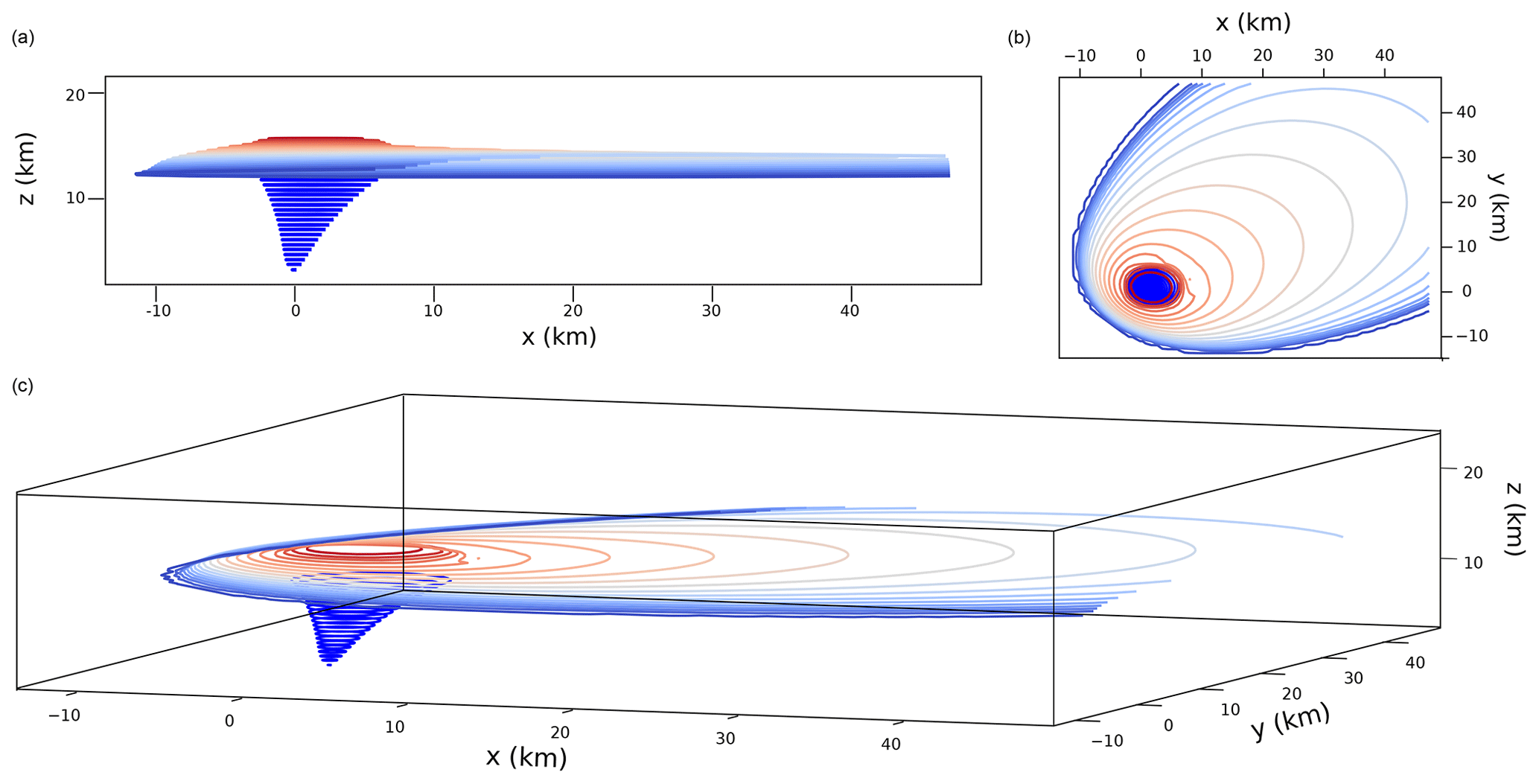
Figure 4 Lateral, top, and oblique views of the plume and the umbrella. The 3-D coordinate system ($x,y,z$) is centered horizontally at the plume base location and vertically at the sea level. Going up the neutral buoyancy level, the plume horizontal sections are calculated by the steady-state model. Above the neutral buoyancy level, the colored contours represent thickness levels of the steady solution computed by the transient umbrella model. The color is not meant to represent cloud thickness but only to better distinguish the contours.

3 Applications

In this section, we present a suite of simulations to highlight the novelties introduced in this version of PLUME-MoM and to constrain model parameters. First, we model the spreading of the umbrella cloud for the eruption of the Calbuco volcano in southern Chile in April 2015 by comparing simulation results with rates of umbrella cloud expansion and upwind spreading derived from satellite observations. This allows us to constrain the coefficient C_D in Eq. (40), controlling the spreading of the umbrella. Then, by using a modified standard atmosphere, an analysis of the effects of wind, atmospheric humidity, and mass flow rate on the upwind spreading of the umbrella cloud is presented.

3.1 April 2015 Calbuco eruption

We present here model results obtained for the two phases of the eruption of the Calbuco volcano in April 2015 (Romero et al., 2016; Castruccio et al., 2016; Van Eaton et al., 2016). Calbuco is one of the most active volcanoes of the southern Chilean Andes, and on the evening of 22 April 2015, for the first time in 43 years, Calbuco erupted, producing a sub-Plinian column with maximum plume heights exceeding 15 km above the vent (Pardini et al., 2018). Preceded by an hour-long period of volcano-tectonic events, the first phase started at 21:04 UTC and lasted approximately 1.5 h, producing tephra dispersed mostly in north and northeast directions and causing a 20 km exclusion zone to be declared. After a 5.5 h break, at 03:54 UTC on 23 April 2015, a second, larger explosive phase begun. This second phase lasted approximately 6 h, with a drop in activity of 1 h approximately 2 h after its onset (Van Eaton et al., 2016). After the second phase, discrete small explosions caused further ash emission up to 2 km height, with a major pulse which resulted in a 4 km high column on 30 April (Romero et al., 2016). Ash from the different phases of the eruption reached Brazil, Chile, Argentina, and Uruguay, causing the canceling of international flights into and out of several major cities in South America.

Table 1 Total grain size distribution for the April 2015 Calbuco eruption (Reckziegel et al., 2019).

Following Reckziegel et al. (2019), for both phases, the total grain size distribution released at the vent (here fixed at an elevation of 2003 m) has been initialized with of a bi-modal distribution with 11 particle classes from −1ϕ to 9ϕ (see Table 1), with densities increasing linearly with ϕ from 2300 to 2700 kg m⁻³. Particle sphericity, mostly affecting the loss of particles through the terminal velocity equation (Textor et al., 2006b), has been fixed to 0.8. Following Van Eaton et al. (2016), we assumed 5 wt % of magmatic water, plus an additional 5 wt % of cooler surface water, possibly associated with the presence of a summit glacier prior to the eruption. The initial temperature of the magmatic mixture has been fixed to 1173 K and, after the mixing with the external water, a temperature of 1006 K has been found for the base of the plume. The initial plume velocity for both phases has been fixed to 250 m s⁻¹, and the radius has been changed for the two phases in order to match the height of the intrusion of the umbrella cloud in the atmosphere and its main spreading direction. This results in a mass eruption rate of 9.54 ×10⁶ kg s⁻¹ for the first phase and 2.02 × 10⁷ kg s⁻¹ for the second one. Varying the initial velocity, while keeping fixed the height of the neutral buoyancy level, produced very similar results in terms of mass eruption rates. The atmospheric profiles used to run the simulations derive from the ECMWF-ERA5 reanalysis dataset. For the two eruptive phases, we extracted geopotential height, atmospheric density, pressure, temperature, specific humidity, and horizontal wind velocity components at the vent location and eruption starting time.

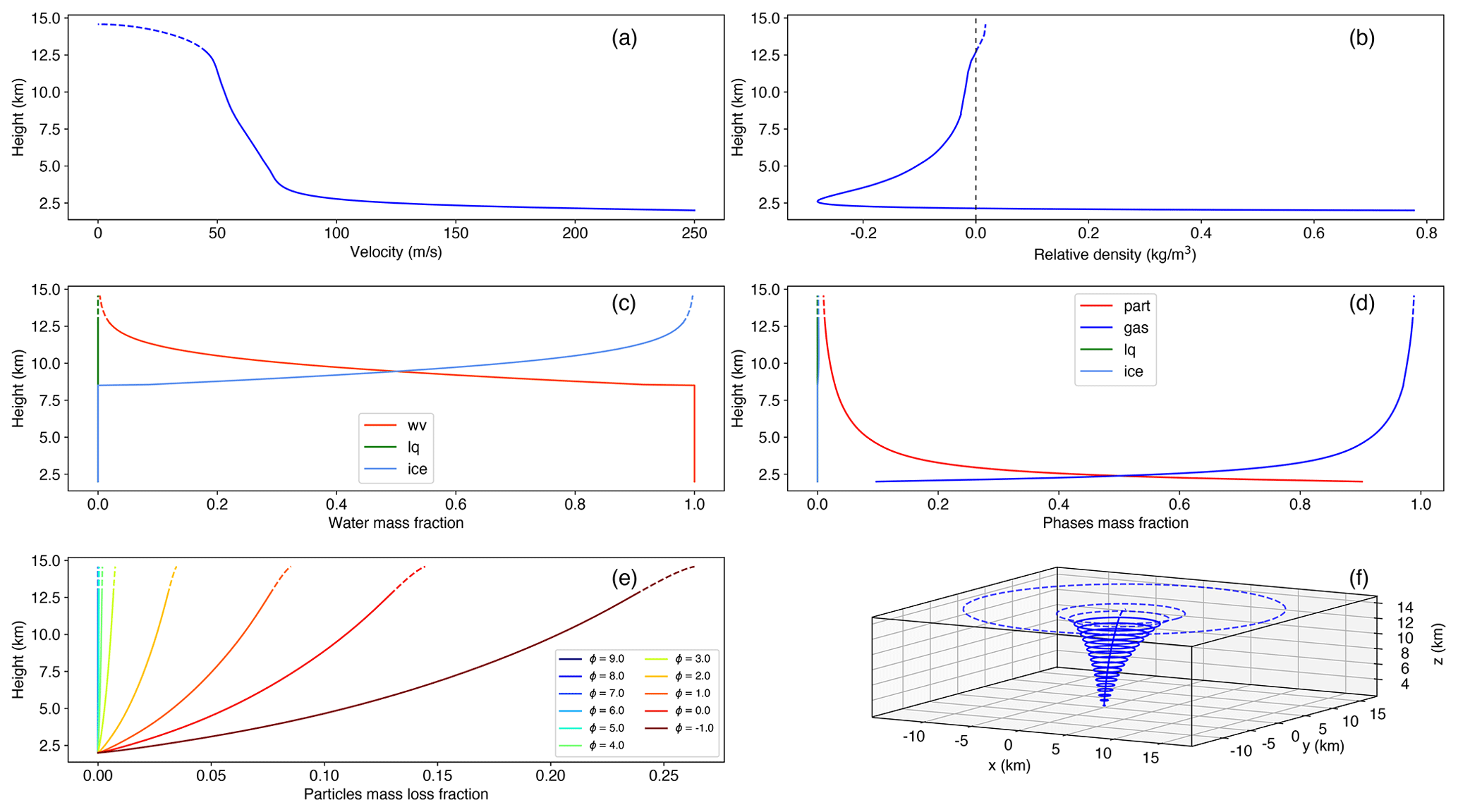
Figure 5 Plume model results for the first phase of the April 2015 Calbuco eruption: (a) velocity profile; (b) relative density, defined as the difference between the density of the volcanic mixture and the density of the surrounding air (with the vertical dashed black line indicating a relative density of zero); (c) relative mass fractions of water phases; (d) mass fractions of particles, gas (water and dry air), liquid water, and ice; (e) relative mass fractions (with respect to the initial amount) of particles lost during the rise for the different bins; (f) three-dimensional view of the plume. Height reported on the left axis of the 2-D plots is measured above sea level. Please note that in all the panels values going up to the neutral buoyancy level are plotted with solid lines, while those corresponding to plume model solutions above the neutral buoyancy level are plotted with dashed lines.

In Fig. 5, some of the plume model outputs obtained for the first phase are reported. In each panel, values below the neutral buoyancy level are plotted with a solid line, while dashed lines represent plume model results above it. Plume velocity (top-left panel) initially decelerates very rapidly in the gas thrust region and then decelerates more gently and almost linearly with height, up to the neutral buoyancy level. Mixture density, because of the large amount of air entrained from the column margin and heated in the gas thrust region, rapidly decreases below atmospheric density, making the plume positively buoyant (see the plot of the relative density in the top-right panel). The water vapor initially present in the rising mixture, with the additional contribution of the moist air entrained in the plume, stays in the gaseous state up to a height above sea level of approximately 8.5 km, above which ice starts to form. At the neutral buoyancy level, almost all the water present in the plume is constituted by ice (middle-left panel). Particles are lost during the rise, but the fraction of the initial amount lost up to the neutral buoyancy level is relatively small, ranging from a maximum of 0.24 for $\mathit{\varphi }=-\mathrm{1}$ to fractions smaller that 0.01 for ϕ≥3. This means that almost all the particles that erupted reach the neutral buoyancy level, and that the initial grain size distribution differs very little from that feeding the umbrella cloud (bottom-left panel). In any case, almost immediately above the vent, due to the large entrainment, the mass of particles, as that of water, rapidly becomes a small fraction of the total mass of the mixture, with the dry air being the more abundant phase (middle-right panel). At the neutral buoyancy level, reached at 12.7 km above sea level, the plume radius is 3935 m (see bottom-right panel) and the mass flow rate injected in the umbrella cloud is 6.64 × 10⁸ kg s⁻¹ (corresponding to a volume flow rate of 2.21×10⁹ m³ s⁻¹). The bottom-right panel presents a 3-D view of the plume, showing the weak bending of the plume axis due to both the moderate wind and the magnitude of the eruption.

Figure 6 Same as Fig. 5 but for the second phase of the April 2015 Calbuco eruption.

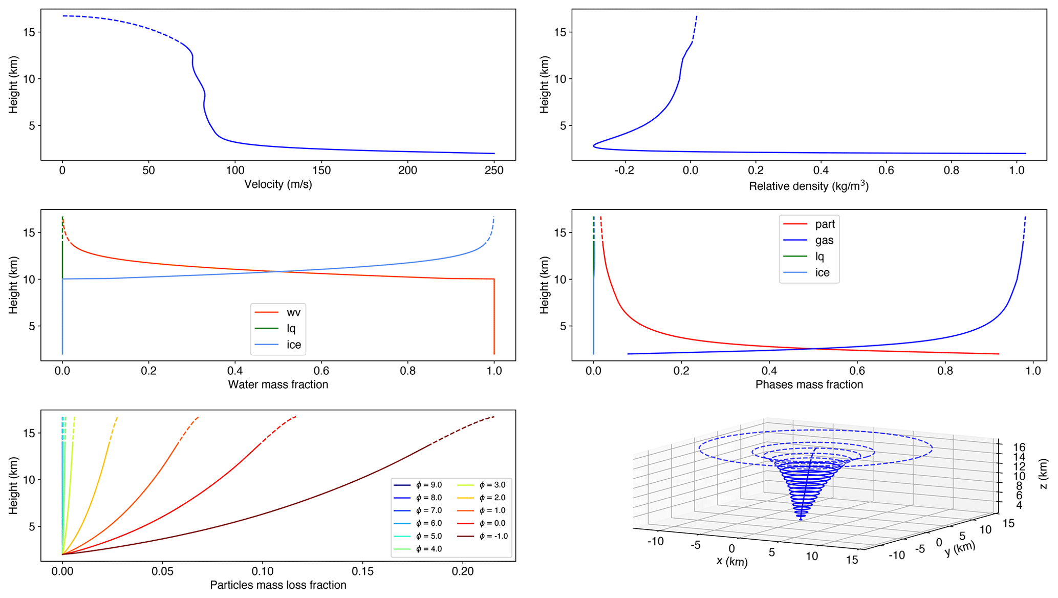
The simulation performed for the second phase produced similar results, and the main output variables are plotted in Fig. 6. For this simulation, the height of the neutral buoyancy level increased to approximately 13.6 km, at which the plume radius is 3814 m, with a mass flow rate injected in the umbrella cloud of 8.38×10⁸ kg s⁻¹ (corresponding to a volume flow rate of 3.22×10⁹ m³ s⁻¹).

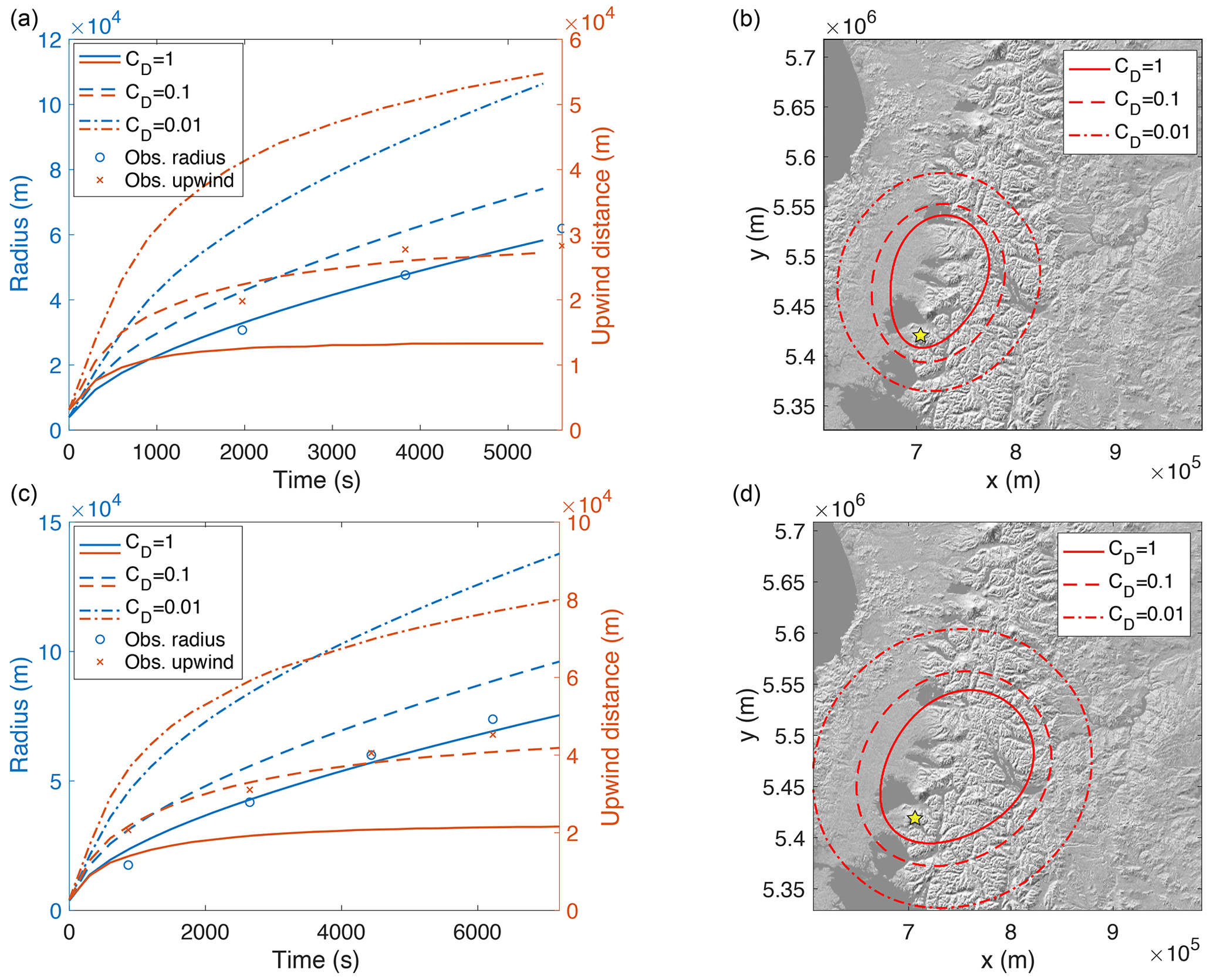
Figure 7 Umbrella cloud spreading for the two initial phases of the April 2015 Calbuco eruption. Panels (a, b) refer to the first phase, while the bottom panels refer to the second phase. Panels (a, c) are plotted the umbrella equivalent radius and the upwind distance versus time, with the markers representing the observations; (b, d) the umbrella cloud edges at the end of the simulations are shown. In all the panels, different lines (solid, dashed, and dash-dotted) represent the three different values of C_D used in this work.

For both phases, the outputs at the neutral buoyancy level of the plume model of PLUME-MoM-TSM (volumetric flow rate, radius, and horizontal velocities) were used as input of the umbrella cloud module. For this application, we varied the drag coefficient C_D of the umbrella cloud model in order to find the value which best reproduced the spreading in the atmosphere observed during the eruption. From the experiments of Abraham et al. (1979), Baines (2013), and Johnson et al. (2015), both inferred coefficients in the range C_D=0.001 to 0.01, while Pouget et al. (2016), by comparing the results of the shallow-water intrusion model developed by Johnson et al. (2015) with satellite data from seven eruptions, better reproduced observations of umbrella cloud structure and morphological evolution with a value C_D=0.1, which was the largest value of the investigated range. Here, three values were tested (C_D= 0.01, 0.1, and 1) by carrying on the simulations for 1.5 and 2 h for the first and second phases, respectively. At each time step, we computed (i) the upwind spreading, defined here as the maximum horizontal distance from the vent in the opposite direction to that of the wind at the neutral buoyancy level; (ii) the radius of a circle with area equivalent to that of the modeled umbrella cloud.

Figure 8 Left panels show the cloud-top IR brightness temperature as retrieved by the NOAA GOES-13 geostationary satellite, channel 4 (images from http://rammb.cira.colostate.edu, last access: 14 February 2021). Right panels show simulated umbrella cloud thickness contours 1.5 h after the onset of phase 1 (top) and phase 2 (bottom), obtained with C_D=0.1. Please note that in the right panels the color scales for the two phases are different.

These values are plotted, at intervals of 300 s, in the left panels of Fig. 7, with blue lines for the equivalent radius and red lines for the upwind distances. In the right panels of Fig. 7, the edges of the umbrella cloud at the end of the simulations are plotted, with different lines for the different values of C_D. From both the left and right panels, we can observe the expected larger spreading of the umbrella cloud for smaller values of C_D. These results highlight the fact that intrusive gravity current dominates in the initial stages of the dispersion of tephra at the neutral buoyancy level and large upwind and crosswind spreadings of the umbrella cloud with respect to the vent location (denoted by a yellow star in the right panels of Fig. 7) are produced also for sub-Plinian eruptions. In order to constrain the value of the drag coefficient, the blue lines in the left panels of Fig. 7 are compared with the series of values for the umbrella radius reported in Van Eaton et al. (2016), obtained by detecting the edge of the umbrella from GOES-13 satellite images and plotted here with blue markers. From the results plotted in the figure, we can see that the values obtained with C_D=1 seem to better match the observations, with a small overestimate at the beginning and a small underestimate at the end of the simulation.

A different result is obtained by analyzing the modeled upwind spreading of the umbrella cloud. First of all, we can see from the red lines in the left panels of Fig. 7 that for values of C_D greater than 0.1, a steady upwind distance is approached at the end of the simulation, and that by changing (increasing or decreasing) the drag coefficient by an order of magnitude, the upwind spreading at the final time changes approximately by a factor of 2. In this case, when model results are compared with the upwind spreading derived from the processing of the observations presented in Van Eaton et al. (2016), represented by the red crosses in the left panels of Fig. 7, we see that the drag coefficient value C_D=0.1 produces the best results. The two different values of C_D obtained by comparing the equivalent radius and the upwind spreading with observational data can be due to the several approximations in the numerical simulations. In particular, the depth-averaged umbrella cloud model uses a constant wind (in time and space), extracted at the vent coordinates and at the neutral buoyancy level from the ECMWF-ERA5 reanalysis data. Thus, while upwind spreading, which is measured close to the vent, is slightly affected by this approximation, the spreading of the whole umbrella cloud (controlling the equivalent radius) could be affected by larger errors, because downwind wind far from the vent can be different from the assumed constant value. Furthermore, we notice that the value C_D=0.1 better agrees with the results presented in Pouget et al. (2016). For these reasons, and because in the rest of the paper we are mostly interested in quantifying the upwind spreading of the umbrella cloud, we use the value C_D=0.1 as reference value. For this value of the drag coefficient, simulated umbrella cloud thicknesses 1.5 h after the onset of each phase are compared in Fig. 8 with cloud-top IR brightness temperatures as retrieved by the NOAA GOES-13 geostationary satellite. First of all, it is important to remark that the images on the left have been cropped from a larger satellite image and have not been reprojected in the same Universal Transverse Mercator (UTM) projection zone used for the right panels (WGS 84/UTM zone 18S), so the two areas represented in the left and right panels do not correspond. In addition, as already stated, model simulations use a constant wind (in time and space), extracted at the vent coordinates and at the neutral buoyancy level, and thus downwind spreading can differ substantially from the real one. In any case, a qualitative comparison shows that the cross-wind spreading of the two phases of the eruption matches well with that predicted by the model. In addition, we observe from the contour plots in the right panels that the larger volumetric flow rate injected at the neutral buoyancy level for the second phase resulted in a thicker cloud, with a total height of column and umbrella of approximately 15.5 and 17.5 km above sea level for the first and second phases, respectively. Also, these values compare well with those reported in Van Eaton et al. (2016).

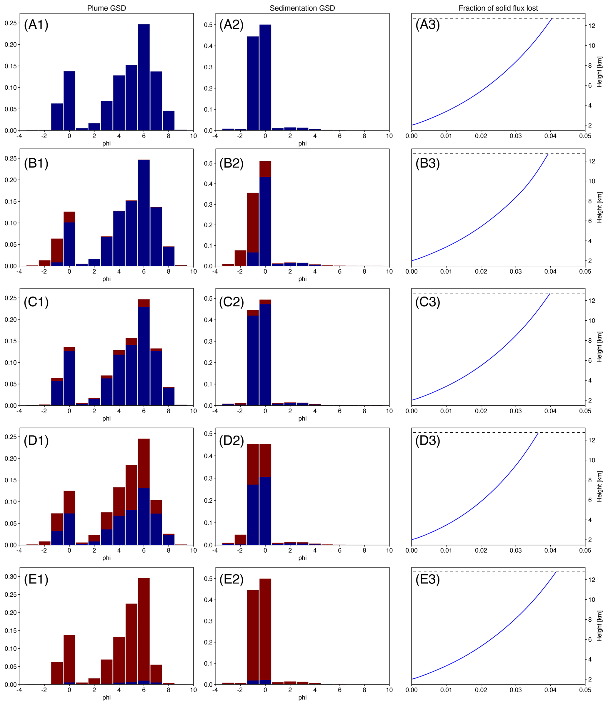
Figure 9 Grain size distributions at the neutral buoyancy level: within the plume (left panels) and released from the plume margins (central panels). The blue bars represent the number of non-aggregated particles, while the maroon bars represent the number of aggregates. The plot on the right panels represent the fraction of solid flux lost from the plume margins because of sedimentation, up to the neutral buoyancy level (represented by the dashed black lines). The results of the simulation without aggregation are plotted in panels (A1) and (A2). The results obtained with the wet aggregation model presented in Costa et al. (2010) are plotted in panels (B1) and (B2). The results obtained with a constant aggregation kernel and values of 10⁻¹⁵, 10⁻¹⁴, and 10⁻¹³ are plotted in panels (C1–C3), (D1–D3), and (E1–E3), respectively.

In the analysis presented so far, we have not accounted for the effect of aggregation. To better understand if aggregation could affect the spreading of the umbrella for this scenario, we repeated the plume rise simulation for the first phase of the April 2015 Calbuco eruption by enabling aggregation between particles and analyzing the changes in the height of the neutral buoyancy level and the grain size distribution of particles still present in the plume and released from its margin at that height. For this set of simulations, two coarser bins ($\mathit{\varphi }=-\mathrm{2},-\mathrm{3}$) with an initial negligible number of particles have been added to the total grain size distribution. This allows for the formation of aggregates larger than the particles present in the original size spectrum. Because we are considering wet aggregation, the density of the aggregates has been fixed to 1500 kg m⁻³ (Costa et al., 2010), resulting in lower settling velocities than the original particles, with the size being equal.

The results of the simulation without aggregation are plotted in the top panels of Fig. 9. The grain size distribution within the plume at the neutral buoyancy level (NBL) is plotted in panel A1 of Fig. 9, the grain size distribution of the particles lost from the plume margins at the same height is plotted in panel A2, and the fraction of the initial total solid flux lost with height (which indicates the number of particles lost from the plume edges during the rise) is shown in panel A3. The grain size distribution at the neutral buoyancy level does not differ significantly from that at the vent, and this is due to the fact that the number of particles lost during the rise is very small (approximately 4 %).

As a first aggregation test, we used a modified version of the wet aggregation kernel introduced in Costa et al. (2010), defined as the product of a collision frequency function and a sticking efficiency function (see Appendix B3). According to this model, to aggregate, a collision must occur between the particles and when that collision occurs the particles must adhere to one another. Collisions between particles are associated with different mechanisms, as Brownian motion, laminar and turbulent fluid shear, and differential settling velocity. Following Costa et al. (2010), all these contributions are considered in the calculation of the collision frequency function. In our formulation, the sticking efficiency depends on the amount of liquid water and ice present in the volcanic plume. For the simulations of the Calbuco eruption, as shown in Fig. 5, only ice forms above a height of 8 km a.s.l. For this reason, aggregation is quite limited and the grain size distributions of the particles within the plume and those particles released from the plume margin at the NBL show very small differences with the simulation without aggregation, and it is limited to the coarser particles. This is mostly due to the fact that the dominant collisional mechanism is the differential settling velocity, which is larger for coarser particles. It is important to note that the neutral buoyancy level differs from that obtained without aggregation by less than 0.1 %, and also the total number of particles lost from the plume does not differ significantly.

In order to better understand the effect of aggregation, we performed additional simulations with a constant kernel, starting from a value of $\mathit{\beta }={\mathrm{10}}^{-\mathrm{15}}$ m³ s⁻¹ up to a value $\mathit{\beta }={\mathrm{10}}^{-\mathrm{13}}$ m³ s⁻¹. The simulation with $\mathit{\beta }={\mathrm{10}}^{-\mathrm{15}}$ m³ s⁻¹ shows small differences compared to that without aggregation, with small numbers of aggregated particles produced (represented in panel B1 of Fig. 9 with the red bars). Because of the adoption of a constant kernel, aggregates form in each bin of the initial grain size distribution. By increasing β by an order of magnitude to a value of 10⁻¹⁴ m³ s⁻¹, the number of aggregates becomes significant (more than 50 % for some bins), and also the relative number of particles released from the plume margins at the neutral buoyancy level differs from that obtained without aggregation. Despite that, we observe that the height of the neutral buoyancy level of the plume does not change, and also the overall bi-modal shape of the total (aggregated and non-aggregated particles) distribution does not change substantially. This is because, with the binary aggregation and the constant aggregation kernel considered here, most of the aggregation occurs “intra-bin”; i.e., it produces an aggregate with a volume, or mass, which belongs to the same bin of particles forming the new aggregate. In fact, for bin sizes of 1 ϕ, and a uniform mass distribution within each bin, the number of smallest particles within a bin is almost 1 order of magnitude smaller than the number of largest particles. Thus, with a constant kernel, aggregation of the smallest particles occurs much frequently, and the aggregate produced from a binary aggregation of these particles produces a new particle with an equivalent diameter (diameter calculated from the mass) still belonging to the same bin. In order to produce a larger change in the particle size distribution in the plume at the neutral buoyancy level, we have to increase the constant kernel to $\mathit{\beta }={\mathrm{10}}^{-\mathrm{13}}$ m³ s⁻¹, for which the fraction of aggregates is close to 97 % of the total mass of particles in the plume (Fig. 9, panels E1 and E2). It is interesting to observe that even with such a large number of aggregates, the total number of particles lost during the rise does not change with respect to the simulation without aggregation, and also the height of the neutral buoyancy level differs from that obtained without aggregation only by 1 m. This result allows us to disregard aggregation for the sensitivity analysis presented in the next section, where the main outputs of the plume module used to initialize the umbrella spreading module are the volumetric flow rate and the height of the gas–particle mixture injected by the plume into the atmosphere at the neutral buoyancy level.

3.2 Umbrella cloud upwind spreading

In this section, we present a sensitivity analysis of the upwind spreading of the umbrella cloud with respect to mass flow rate and to some parameters characterizing the meteorological profile above the vent. This study builds on the ideas of Carey and Sparks (1986), where the ratio of upwind spreading to the amount of axial displacement at the neutral buoyancy level was analyzed, with results based on theoretical and empirical information on column behavior. With respect to the previous section, where atmospheric profiles used to run the simulations were derived from the ECMWF-ERA5 reanalysis data, the simulations presented here employ atmospheric profiles of pressure, temperature, and density modified from the International Standard Atmosphere (ISA) model. This model provides a common reference for temperature and pressure at various altitudes, and it is based on the subdivision of the atmosphere in layers where the absolute temperature T_atm against geopotential altitude h (i.e., the vertical coordinate referenced to Earth's mean sea level) is assumed to vary linearly. Geopotential and orthometric heights differ little for low terrestrial atmosphere (Daidzic, 2019), and for this reason we can assume a linear dependence of temperature also against orthometric height (i.e., the distance of a point along the plumb line to the geoid). In the following, as common in meteorology, we refer to the negative value of the rate of temperature change with altitude using the term “lapse rate”, and we use for it the notation of Γ. Once the bottom values and the lapse rate are known in an atmospheric layer, pressure, temperature, and density profiles within the layer can be calculated by solving simultaneously the equation for vertical pressure gradient resulting from hydrostatic balance, the equation for temperature, and the ideal gas law:

$$\begin{array}{}\text{(43)}& \left\{\begin{array}{l}\frac{\partial P_{\mathrm{atm}}}{\partial z}=-{\mathit{\rho }}_{\mathrm{atm}}\left(z\right)g\\ \frac{\partial T_{\mathrm{atm}}}{\partial z}=-{\mathrm{\Gamma }}_{\mathrm{atm}}\\ {\mathit{\rho }}_{\mathrm{atm}}=\frac{P_{\mathrm{atm}}}{R{T}_{\mathrm{atm}}},\end{array}\right.\end{array}$$

where R is the specific gas constant of the atmosphere, which can vary with humidity. When the option for a modified standard atmosphere is selected in PLUME-MoM-TSM, the first two equations are added to the set of ordinary differential equations solved numerically by the model, and the last one is employed to calculate explicitly the right-hand term of the first equation.

Table 2 International Standard Atmosphere (ISA) layers and lapse rates up to 71 km geopotential altitude.

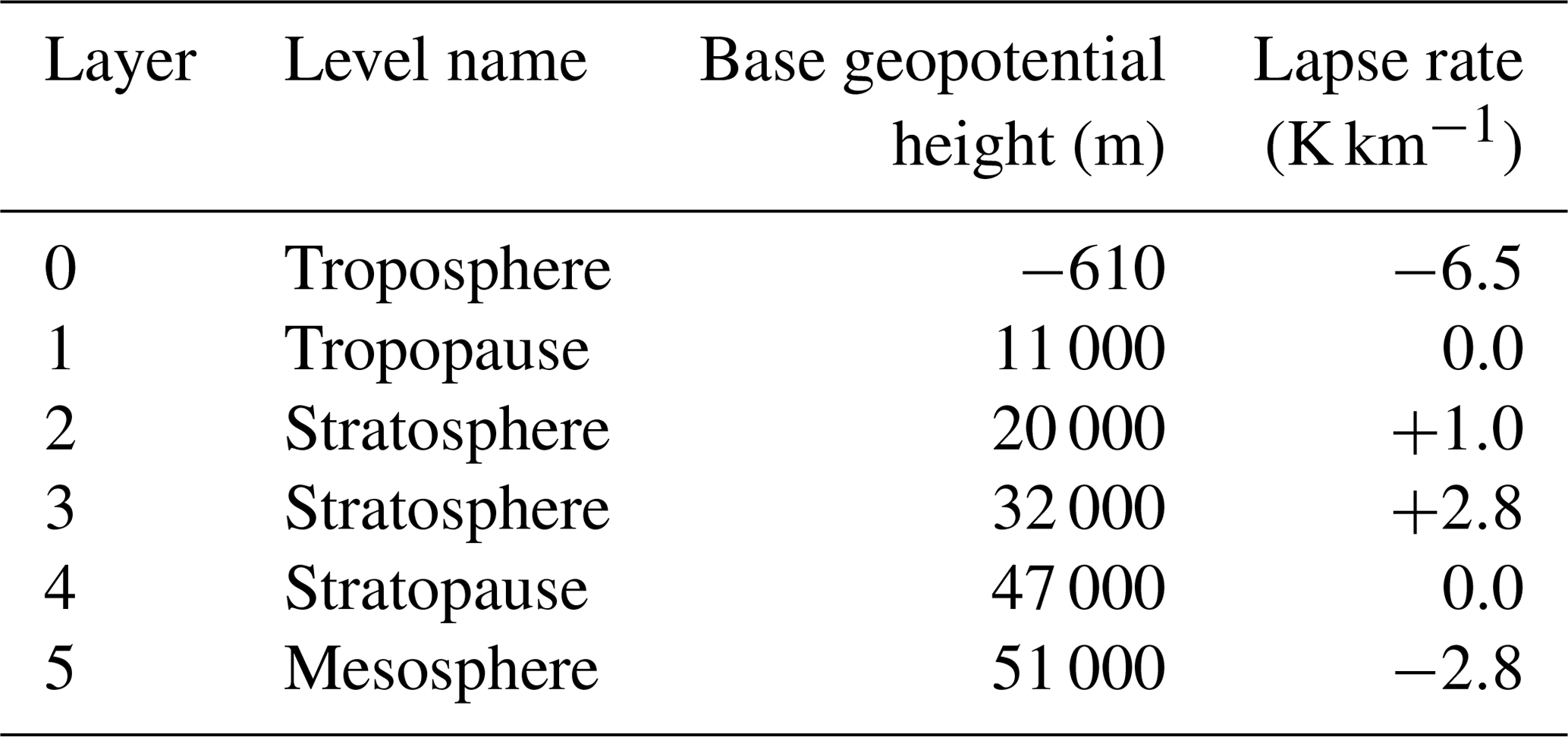
ISA lapse rates (see Table 1) do not account for humidity effects and air is assumed to be dry, and the specific gas constant used in the ideal gas law is that of dry air (R=R_air). For this reason, when humidity is considered, appropriate corrections to the atmospheric profiles given by the ISA model need to be introduced. Moist unsaturated air cools with height at a slightly lower rate than dry air (Dutton, 2002), and in this work we adopt the following lapse rate correction to account for the presence of water vapor, as proposed in Daidzic (2019):

$$\begin{array}{}\text{(44)}& {\mathrm{\Gamma }}_{\mathrm{atm}}={\mathrm{\Gamma }}_{\mathrm{d}}\left(\mathrm{1}-\mathrm{0.856}s{h}_{\mathrm{atm}}\right),\end{array}$$

where Γ_atm and Γ_d are the moist and dry atmospheric lapse rates, respectively. According to Ahrens (2012), the average specific humidity in the lower troposphere ranges from 0.004 kg kg⁻¹ at 60^∘ (north or south) to 0.018 kg kg⁻¹ at the Equator, and its value exponentially decreases to values lower than 10⁻⁵ kg kg⁻¹ above the tropopause. It follows that the sensitivity of lapse rates to the specific humidity value is minimal in the lower troposphere and negligible above it.

Density of moist atmosphere also varies with water content, and the relationship between dry and moist air densities can be written as

$$\begin{array}{}\text{(45)}& {\mathit{\rho }}_{\mathrm{atm}}={\displaystyle \frac{{\mathit{\rho }}_{\mathrm{d}}}{\mathrm{1}+\left(\frac{R_{\mathrm{wv}}}{R_{\mathrm{air}}}-\mathrm{1}\right)s{h}_{\mathrm{atm}}}},\end{array}$$

where R_wv and R_air are the gas constants of water vapor and air, respectively.

With these equations, ISA lapse rates Γ_d and density ρ_d are corrected for the presence of humidity, and it is possible to solve the system of Eq. (43) for the modified pressure and temperature profiles. The specific humidity profile used in the simulations presented here has been derived from the data presented in Anderson et al. (1986), providing the values at the boundaries between the atmospheric layers, while values at the bottom of the troposphere have been varied in the range 0.004–0.018 kg kg⁻¹. Inside each layer, the logarithm of specific humidity is assumed to vary linearly.

In this work, we also assume the wind speed to be a continuous function of height which varies linearly in several layers. Observations indicate that on average the wind speed profile has local minima at altitudes of about 20 km and about 90 km, where air masses are relatively stationary, and local maxima at altitudes of about 11 and 70 km (Modica et al., 2007; Brasefield, 1954). While quite a wide range of values is observed for the first maximum at the tropopause, the value of the wind speed at 70 km varies less, and a speed of 65 m s⁻¹ is assumed in this work. For the wind speed minimum at 20 km altitude, we fix a value of 10 m s⁻¹. With these assumptions, the relevant atmospheric profiles obtained for a moist atmosphere and with a wind speed of 20 m s⁻¹ at 11 km are plotted in Fig. 10, where the red markers in the last two panels denote the values we varied for the sensitivity analysis.

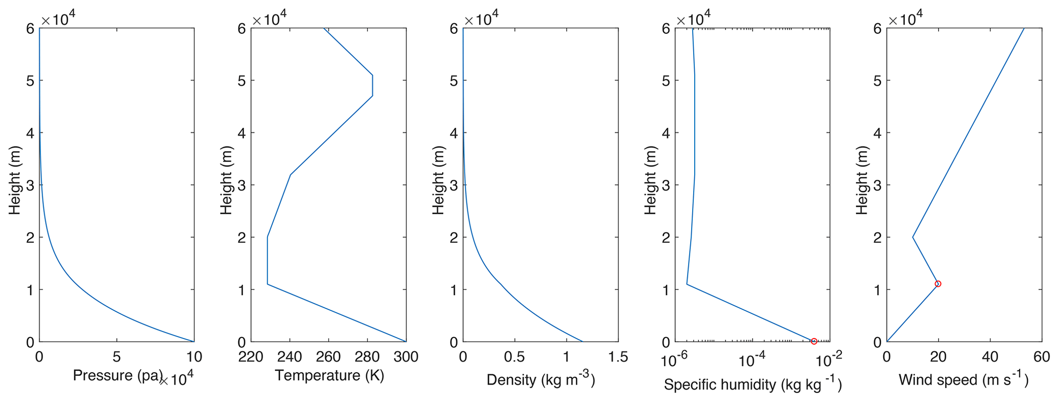
Figure 10 Atmospheric profiles for a dry atmosphere with a 20 m s⁻¹ wind speed at the tropopause (11 km a.s.l.). The red markers denote the values that can be changed in the modified standard atmosphere adopted in the model. The first three profiles (pressure, temperature, and density) also change when the specific humidity at the sea level is changed.

Maximum upwind spreading of the umbrella cloud with respect to vent location represents an important information that coupled plume and umbrella models or fully three-dimensional models (Cerminara et al., 2016; Suzuki and Koyaguchi, 2009) can provide. It has been noted that using only the output of integral plume models as the source of VATD models generally underestimates the upwind deposition patterns of volcanic ash, and corrections accounting for the initial spreading of the umbrella as a gravity current result in a better agreement of ash distribution close to the eruptive source (Costa et al., 2013; Webster et al., 2020).

Most of the work done so far to couple the spreading of the umbrella cloud with advection–diffusion–sedimentation models focused on large events such as the 1991 Pinatubo eruption, with a mass flow rate of the order of 10⁹ kg s⁻¹. Less work has been devoted to smaller scenarios, and for this reason we focus here on lower values of mass flow rate in order to gain a better understanding of the relationship between mass flow rate, wind speed, and upwind spreading. It is well known that upwind spreading increases with increasing mass flow rate and decreasing wind, but a quantitative relationship between them is unknown. Here, we varied three input parameters of the model: (1) the decadic logarithm of mass flow rate in the range 6–8 (i.e., $\dot{m}={\mathrm{10}}^{\mathrm{6}}$–10⁸ kg s⁻¹), adjusted by changing vent diameter; (2) the wind speed at the tropopause in the range 35–80 m s⁻¹; and (3) the specific humidity at sea level in the range 0.004–0.018 kg kg⁻¹. A uniform probability has been assigned to all the input variables and the space of parameters has been sampled with Latin hypercube sampling generating 700 elements. The other main input parameters used for this analysis are listed in Table 3. As previously stated, aggregation is disregarded. In addition, as shown in de' Michieli Vitturi et al. (2015), also the initial total grain size distribution has a minimal control on plume height, and consequently on upwind umbrella spreading. For this reason, it has been kept fixed for all the simulations. As for the previous application, settling of particles from the plume edges is considered, and the settling velocity model from Textor et al. (2006b) is adopted (see Appendix B2 for more details).

Table 3 Relevant input parameters of the plume model fixed for all the simulations of the sensitivity analysis.

For each simulation, the horizontal upwind distance from the vent of the umbrella cloud has been calculated from the output of umbrella spreading module (when a steady value is reached), and correlation plots with the three input parameters are presented in the first three panels of Fig. 11, where each red dot represents a different simulation. In general, we observe increasing upwind spreading with increasing mass eruption rate and decreasing wind speed at the tropopause, while the relative humidity does not seem to affect it. For a fixed value of the input parameters on the x axis, the vertical spreading of the red dot cloud is associated with variations in the other input parameters. Each black line represents the average of the upwind spreading values at a given input value.

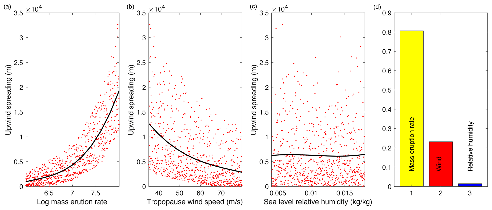
Figure 11 Upwind spreading of the umbrella cloud as a function of input parameters (a–c) and main sensitivity indices (d). In the first three panels, each red dot represents a different simulation, whereas the black lines represent the mean of the output parameter at a given input value. For a fixed value of the input parameters on the x axis of a plot, the vertical spreading of the results is associated with variations in the other input parameters.

The global sensitivity of the upwind spreading with respect to the three input parameters has been computed by using a variance-based method (Saltelli et al., 2010; Scollo et al., 2008; de' Michieli Vitturi et al., 2016). If we denote the output parameter of interest with Y and the input parameters considered with x_i, the main sensitivity index S_i, also called the Sobol index, expresses the fraction of the variability in the output Y that is reduced when the value of the input x_i is fixed. It is calculated by

$$\begin{array}{}\text{(46)}& S_i={\displaystyle \frac{{\mathrm{Var}}_{x_i}\left[Y|x_i\right]}{\mathrm{Var}\left(Y\right)}}.\end{array}$$

The values of the Sobol index are shown in the bar plot presented in the right panel of Fig. 11. The largest value is obtained for the sensitivity with respect to the mass flow rate (yellow bar), with a smaller sensitivity with respect to the wind speed at the tropopause (red bar) and a negligible effect of the specific humidity at sea level (blue bar). This highlights the fact the upwind spreading is mostly controlled by the first two parameters.

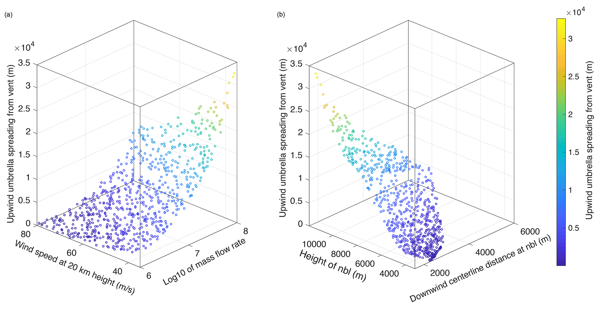
Figure 12 Upwind spreading of the umbrella cloud as a function of wind speed at tropopause and mass flow rate (a) and plume model output parameters (b). Please note that in the left panel also the specific humidity at sea level is varied, without producing significant variations in the upwind spreading.

For this reason, we plotted in Fig. 12 the maximum upwind spreading as a function of the logarithm of the mass flow rate and the tropopause wind speed only, highlighting a potential power-law dependence of the spreading on the two input variables. In fact, if we denote with d_up the upwind spreading and with $\dot{m}$ and v the mass flow rate and the tropopause wind speed, respectively, we can write

$$\begin{array}{}\text{(47)}& d_{\mathrm{up}}=a{\displaystyle \frac{({\log }_{\mathrm{10}}\dot{m}{)}^b}{v^c}}.\end{array}$$

A least-squares minimization procedure gives $a=\mathrm{1.22}\times {\mathrm{10}}^{-\mathrm{3}}$, b=10.75, and c=1.453 as optimal values for the fitting parameters, with a coefficient of determination of R²=0.987 and a square root of the variance of the residuals of 680.8 m. With these values, the relationship expressed by Eq. (47) gives an estimation of the upwind spreading once the mass flow rate and the tropopause wind speed are known. While from a modeling perspective this represents an interesting result, it is not always applicable, because the input values needed to compute the spreading cannot be observed directly. For this reason, we plotted in the right panel of Fig. 12 the upwind umbrella distance as a function of the height of the NBL and the downwind horizontal distance of the centerline at the NBL from the vent, both extracted from the output of PLUME-MoM-TSM plume module. As expected, upwind spreading decreases with increasing bending of the column (expressed by the downwind distance of the centerline from the vent), because the bending is associated with wind intensity. On the contrary, upwind spreading increases with increasing height of the intrusion in the atmosphere. Also in this case there is a power-law dependence of the upwind spreading d_up on the two input variables and, if we denote with h and d_down the NBL height and the downwind distance of the centerline from the vent (measured at the NBL), respectively, we can write

$$\begin{array}{}\text{(48)}& d_{\mathrm{up}}=A{\displaystyle \frac{h^B}{(d_{\mathrm{down}}{)}^C}}.\end{array}$$

In this case, the least-squares minimization procedure gives $A=\mathrm{9.055}\times {\mathrm{10}}^{-\mathrm{6}}$, B=2.993, and C=0.806 as optimal values for the fitting parameters, with a coefficient of determination of R²=0.985 and a square root of the variance of the residuals of 719.5 m. The results of this fitting and the residuals are shown in Fig. 13, showing that the largest absolute error is obtained for the larger values of the upwind spreading. In any case, these errors of the fitting result in an overestimation of the modeled upwind spreading of less than 5 %. It is important to remark that the fitting parameters we obtained are valid for the range of tropopause wind speeds (35–80 ms⁻¹) and mass flow rates (10⁶–10⁸ kg s⁻¹) investigated in this analysis, and that extrapolations outside these ranges should be avoided.

Figure 13 Exponential fitting of upwind spreading vs. neutral buoyancy level height and downwind displacement of the plume axis at the same height. A contour plot is shown in panel (a), while on the right 3-D views of the fitting surface (b) and the residuals of the fitting (c) are shown. The black dots in panels (a–c) represent PLUME-MoM-TSM results.

This second relationship, from an operational point of view, may be more useful. On one hand, the two input values are produced by all plume integral models, and in this way a correction can be applied to obtain the upwind spreading without the need of an umbrella cloud spreading model. On the other hand, the input values are also observable data than can be estimated with monitoring techniques, allowing us to have an immediate initial estimation of the upwind spreading, and thus of the upwind area potentially affected by the presence of ash, once the volcanic column is observed.

The results presented here are consistent with those discussed in Carey and Sparks (1986), who showed that for very weak plumes no true umbrella cloud forms and a direct coupling of column and dispersal models is appropriate, while, for columns able to reach the tropopause, upwind spreading is significant and an umbrella model is required. Further studies will address this point by considering the uncertainty associated with additional input parameters of the models. We also remark that the values of the upwind spreading presented here are strongly dependent on the drag coefficient C_D, in this analysis fixed at 0.1, and that the lower values suggested by Baines (2013) and Johnson et al. (2015) would produce a larger upwind spreading of the umbrella cloud. Additional simulations we performed (not shown here) suggest that a decrease of the drag coefficient of 1 order of magnitude results approximately in doubling the upwind spreading distance. Finally, it is worth noting that in this analysis we have not varied some of the parameters which can have a large control on the eruptive column, such as the initial water content and temperature (de' Michieli Vitturi et al., 2016; Costa et al., 2016).

4 Conclusions

PLUME-MoM-TSM, like all the integral models of volcanic plumes, is based on important simplifications, from the steadiness of the plume to the 1-D formulation. For this reason, it cannot describe the details of the complex transient and 3-D dynamics of turbulent volcanic plumes. Despite that, integral models are able to predict column heights and neutral buoyancy levels consistent with those calculated by 3-D models (Costa et al., 2016). This result, coupled with the fact that integral models require few seconds to run, pushes toward further development of these models. In this work, we have presented PLUME-MoM-TSM, a new version of the volcanic plume model PLUME-MoM described in de' Michieli Vitturi et al. (2015) and based on the method of moments for the description of the particle distributions. With respect to the previous version, where a finite set of moments of the total grain size distribution was tracked, here the adoption of the two-size moment allowed us to model the evolution of the mass and the number of particles associated with each single bin of the distribution. A first important consequence is that, with such an approach, it is possible to use PLUME-MoM-TSM outputs as the input of VATD models. In addition, the method used in this work to describe the grain size distribution allows for the solution of the full Smoluchowski coagulation equation and thus to model accurately particle aggregation. We applied here the two-size moment method to the steady-state integral equations for the plume, but the procedure described is general and the code has a modular structure, which make it easy to port the procedure to other Eulerian models for transport of volcanic ash in the atmosphere.

PLUME-MoM-TSM also accounts for phase changes of water, resulting in the formation of liquid water or ice inside the plume, and it includes a module for the spreading of the umbrella cloud as a gravity current. These new features have been tested by applying the model to the April 2015 eruption of the Calbuco volcano in Chile, allowing us to calibrate the drag coefficient of the umbrella cloud depth-averaged model and to quantify the effect of wet aggregation on model results. The analysis shows that aggregation has a minimal control on plume characteristics and on the loss of particles from its margins. We observe that dry aggregation could produce different results, because the aggregates would have lower densities and thus lower settling velocity, strongly affecting the deposition pattern from the rising plume. In addition, we remark that most aggregates that have been mapped in proximal fallout (Self, 1983; Sisson, 1995; Wallace et al., 2013) and produced in shaker-pan experiments (Van Eaton et al., 2012) have a size distribution narrower than that produced by the aggregation kernel we adopted. This suggests that in the future the model could be updated with new collision and sticking kernels, informed by laboratory experiments and data coming from fallout deposits.

Finally, a sensitivity analysis provided a relationship between mass flow rate, wind speed at the tropopause, and maximum upwind spreading of the umbrella cloud, and also between observable parameters quantifying plume bending (height of the neutral buoyancy level and downwind displacement of the plume axis at the same height) and the umbrella upwind spreading. These results are in agreement and extend those presented in Carey and Sparks (1986), and provide important information for both modelers and observatories, even if further studies are necessary to extend the analysis to more general initial vent conditions.

Appendix A: Reconstruction from moments

The TSM method is based on the reconstruction of the number density function from the moments, which are updated by the solution of the plume equations. We provide here the details of the TSM reconstruction of the number density function ${\stackrel{\mathrm{̃}}{\mathit{\eta }}}_k\left(m\right)$ from the two moments (N_k and M_k) in the mass interval $[m_{k-\mathrm{1}},m_k]$.

The linear reconstruction ${\stackrel{\mathrm{̃}}{\mathit{\eta }}}_k\left(m\right)$ defined by Eq. (10), CASE 2, satisfies the conditions ${\stackrel{\mathrm{̃}}{\mathit{\eta }}}_k^{\left(\mathrm{0}\right)}=N_k$ and ${\stackrel{\mathrm{̃}}{\mathit{\eta }}}_k^{\left(\mathrm{1}\right)}=M_k$ for the following values of α_k and β_k:

$$\begin{array}{ll}{\displaystyle }& {\displaystyle }{\mathit{\alpha }}_k={\displaystyle \frac{\mathrm{2}(N_k{m}_{k-\mathrm{1}}-\mathrm{3}{M}_k+\mathrm{2}{N}_k{m}_k)}{(m_k-m_{k_{\mathrm{1}}}{)}^{\mathrm{2}}}},\\ {\displaystyle }& {\displaystyle }{\mathit{\beta }}_k=-{\displaystyle \frac{\mathrm{2}(\mathrm{2}{N}_k{m}_{k-\mathrm{1}}-\mathrm{3}{M}_k+N_k{m}_k)}{(m_k-m_{k_{\mathrm{1}}}{)}^{\mathrm{2}}}}.\end{array}$$

We observe now that the linear reconstruction is a physical approximation of a number density function only if its values are positive in the interval $[m_{k-\mathrm{1}},m_k]$, and this can be verified by calculating the values of ${\stackrel{\mathrm{̃}}{\mathit{\eta }}}_k\left(m\right)$ at m_k−1 and m_k.

If for the linear reconstruction given by CASE 2 and by the values of α_k and β_k defined above it holds ${\stackrel{\mathrm{̃}}{\mathit{\eta }}}_k\left(m_{k-\mathrm{1}}\right)<\mathrm{0}$, then we switch to Eq. (10), CASE 1. In this case, the conditions ${\stackrel{\mathrm{̃}}{\mathit{\eta }}}_k^{\left(\mathrm{0}\right)}=N_k$ and ${\stackrel{\mathrm{̃}}{\mathit{\eta }}}_k^{\left(\mathrm{1}\right)}=M_k$ are satisfied for the following values of α_k and γ_k:

$$\begin{array}{ll}{\displaystyle }& {\displaystyle }{\mathit{\alpha }}_k={\displaystyle \frac{N(M_k-N_k{m}_k)}{(m_{k-\mathrm{1}}-m_k)(M_k-N_k{m}_{k-\mathrm{1}})}},\\ {\displaystyle }& {\displaystyle }{\mathit{\gamma }}_k={\displaystyle \frac{N_k{m}_{k-\mathrm{1}}-\mathrm{2}{M}_k+N_k{m}_k}{M_k-N_k{m}_{k-\mathrm{1}}}}.\end{array}$$

Conversely, if for the linear reconstruction given by CASE 2 and by the values of α_k and β_k defined above it holds ${\stackrel{\mathrm{̃}}{\mathit{\eta }}}_k\left(m_k\right)<\mathrm{0}$, then we switch to Eq. (10), CASE 3. In this case, the conditions ${\stackrel{\mathrm{̃}}{\mathit{\eta }}}_k^{\left(\mathrm{0}\right)}=N_k$ and ${\stackrel{\mathrm{̃}}{\mathit{\eta }}}_k^{\left(\mathrm{1}\right)}=M_k$ are satisfied for the following values of β_k and γ_k:

$$\begin{array}{ll}{\displaystyle }& {\displaystyle }{\mathit{\beta }}_k={\displaystyle \frac{N(M_k-N_k{m}_{k-\mathrm{1}})}{(m_{k-\mathrm{1}}-m_k)(M_k-N_k{m}_k)}},\\ {\displaystyle }& {\displaystyle }{\mathit{\gamma }}_k={\displaystyle \frac{N_k{m}_{k-\mathrm{1}}-\mathrm{2}{M}_k+N_k{m}_k}{M_k-N_k{m}_k}}.\end{array}$$

We observe that we cannot have both ${\stackrel{\mathrm{̃}}{\mathit{\eta }}}_k\left(m_{k-\mathrm{1}}\right)<\mathrm{0}$ and ${\stackrel{\mathrm{̃}}{\mathit{\eta }}}_k\left(m_k\right)<\mathrm{0}$ because of the positivity of the moments M_k and N_k.

Appendix B: Constitutive equations

B1 Water-phase transition

For the partition of water in the gas, liquid, and solid phases, three different cases are considered: T_mix≥T_ref, $T_{\mathrm{ref}}-\mathrm{40}<T_{\mathrm{mix}}<T_{\mathrm{ref}}$, and $T_{\mathrm{mix}}\le T_{\mathrm{ref}}-\mathrm{40}$, where T_ref is the reference temperature of 273.15 K. Starting from the first case, we solve for the unknown variables (mass fraction of the different phases) and we check if their values are consistent with the hypothesis of thermal and mechanical equilibrium between all phases. If the equilibrium is not possible, we skip to a different case.

1. For T_mix≥T_ref, water can be in vapor and liquid form only and T_mix is given by

   $$\begin{array}{}\text{(B1)}& T_{\mathrm{mix}}={\displaystyle \frac{H-x_{\mathrm{lw}}\left(h_{\mathrm{lw}\mathrm{0}}-C_{\mathrm{lw}}{T}_{\mathrm{ref}}\right)-x_{\mathrm{wv}}\left(h_{\mathrm{wv}\mathrm{0}}-C_{\mathrm{wv}}{T}_{\mathrm{ref}}\right)}{x_{\mathrm{da}}{C}_{\mathrm{atm}}+x_{\mathrm{s}}{C}_{\mathrm{s}}+x_{\mathrm{lw}}{C}_{\mathrm{lw}}+x_{\mathrm{wv}}{C}_{\mathrm{wv}}+x_{\mathrm{vg}}{C}_{\mathrm{vg}}}}.\end{array}$$

   Following Folch et al. (2016), for T≥29.65 K, the saturation pressure of vapor over liquid (e_l) depends on mixture temperature in the following way:

   $$\begin{array}{}\text{(B2)}& e_{\mathrm{l}}\left(T_{\mathrm{mix}}\right)=\mathrm{611.2}\exp \left(\mathrm{17.67}{\displaystyle \frac{\left(T_{\mathrm{mix}}-\mathrm{273.16}\right)}{\left(T_{\mathrm{mix}}-\mathrm{29.65}\right)}}\right).\end{array}$$

   At equilibrium condition, when both liquid water and vapor are present, it must hold:

   $$\begin{array}{}\text{(B3)}& {\mathrm{\Delta }}_{\mathrm{wv}}\equiv P_{\mathrm{wv}}-e_l=\mathrm{0},\end{array}$$

   where both terms can be written as functions of x_wv, by appropriately combining Eqs. (33), (34), (B1), and (B3).

   Before trying to solve Eq. (B3), we consider the two extreme values – x_wv=0 (liquid only) and x_wv=x_w (vapor only) – in order to check if they are compatible with the condition T_mix≥T_ref. If ${\mathrm{\Delta }}_{\mathrm{wv}}{|}_{x_{\mathrm{wv}}=x_{\mathrm{w}}}<\mathrm{0}$ and $T_{\mathrm{mix}}{|}_{x_{\mathrm{wv}}=x_{\mathrm{w}}}\ge T_{\mathrm{ref}}$, the plume is undersaturated and there is no water vapor condensation (x_w=x_wv). If ${\mathrm{\Delta }}_{\mathrm{wv}}{|}_{x_{\mathrm{wv}}=\mathrm{0}}>\mathrm{0}$ and $T_{\mathrm{mix}}{|}_{x_{\mathrm{wv}}=\mathrm{0}}>T_{\mathrm{ref}}$, all the water is in liquid form (x_w=x_lw). Otherwise, we apply a bisection iterative method to solve Eq. (B3) for x_wv in the interval [0,x_w]. Once the solution is obtained, we check if the corresponding temperature, as given by Eq. (B1), is ≥T_ref. If this is not the case, T_mix must be less than T_ref.

2. For $T_{\mathrm{mix}}\le T_{\mathrm{ref}}-\mathrm{40}$, water can be in vapor and ice form only and the temperature of the eruptive mixture can be computed as

   $$\begin{array}{}\text{(B4)}& T_{\mathrm{mix}}={\displaystyle \frac{H-x_{\mathrm{wv}}\left(h_{\mathrm{wv}\mathrm{0}}-C_{\mathrm{wv}}{T}_{\mathrm{ref}}\right)}{x_{\mathrm{da}}{C}_{\mathrm{atm}}+x_{\mathrm{s}}{C}_{\mathrm{s}}+x_{\mathrm{wv}}{C}_{\mathrm{wv}}+x_{\mathrm{i}}{C}_{\mathrm{i}}+x_{\mathrm{vg}}{C}_{\mathrm{vg}}}}.\end{array}$$

   We follow the procedure adopted for T_mix≥T_ref with the difference of considering the equations holding for a mixture containing water as vapor and ice. From Folch et al. (2016), the saturation pressure of vapor over ice (e_s) is a function of mixture temperature T_mix as

   $$\begin{array}{}\text{(B5)}& \begin{array}{rl}& e_{\mathrm{s}}\left(T_{\mathrm{mix}}\right)\\ & =\mathrm{611.22}\times {\mathrm{10}}^{-\mathrm{9.097}\left(\frac{\mathrm{273.16}}{T_{\mathrm{mix}}}-\mathrm{1}\right)-\mathrm{3.566}{\log }_{\mathrm{10}}\left(\frac{\mathrm{273.16}}{T_{\mathrm{mix}}}\right)+\mathrm{0.876}\left(\mathrm{1}-\frac{T_{\mathrm{mix}}}{\mathrm{273.16}}\right)}.\end{array}\end{array}$$

   At equilibrium, when both vapor and ice are present, it must hold:

   $$\begin{array}{}\text{(B6)}& {\mathrm{\Delta }}_{\mathrm{wv}}\equiv P_{\mathrm{wv}}-e_{\mathrm{s}}=\mathrm{0},\end{array}$$

   where P_wv and e_s can be written as functions of x_wv only, by appropriately combining Eqs. (33), (34), (B5), and (B4). Again, before solving Eq. (B6), we examine the two extreme cases – x_wv=0 (ice only) and x_wv=x_w (vapor only) – and we check if the corresponding temperature as evaluated from Eq. (B4) is less than T_ref−40. In the case of ${\mathrm{\Delta }}_{\mathrm{wv}}{|}_{x_{\mathrm{wv}}=x_{\mathrm{w}}}<\mathrm{0}$ and $T_{\mathrm{mix}}{|}_{x_{\mathrm{wv}}=x_{\mathrm{w}}}<T_{\mathrm{ref}}-\mathrm{40}$, the plume is undersaturated and water is in vapor form only (x_w=x_wv). On the contrary, in the case of ${\mathrm{\Delta }}_{\mathrm{wv}}{|}_{x_{\mathrm{wv}}=\mathrm{0}}>\mathrm{0}$ and $T_{\mathrm{mix}}{|}_{x_{\mathrm{wv}}=\mathrm{0}}<T_{\mathrm{ref}}-\mathrm{40}$, all the water is present as ice (x_w=x_i).

   If equilibrium conditions can not be obtained for the two extreme cases, we solve Eq. (B6) for x_w by applying a bisection procedure in the interval [0,x_w] and we check if the corresponding temperature given by Eq. (B4) is $<T_{\mathrm{ref}}-\mathrm{40}$.

3. For $T_{\mathrm{ref}}-\mathrm{40}<T_{\mathrm{mix}}<T_{\mathrm{ref}}$, water can be in vapor, liquid, and ice form. Following Mastin (2007) and references therein, we assume that in this range of temperatures liquid and ice coexist but not in equilibrium, with liquid water present in a subcooled state to temperatures well below freezing. In this case, specific mixture enthalpy can be computed from Eq. (27) as a function of mixture temperature only. Indeed, we show in the following that water mass fractions can be written as functions of T_mix. Water vapor mass fraction is computed by inverting Eq. (34) as

   $$\begin{array}{}\text{(B7)}& x_{\mathrm{wv}}\left(T_{\mathrm{mix}}\right)=-{\displaystyle \frac{\left(\frac{x_{\mathrm{da}}}{m{w}_{\mathrm{da}}}+\frac{x_{\mathrm{vg}}}{m{w}_{\mathrm{vg}}}\right)n_{\mathrm{wv}}m{w}_{\mathrm{wv}}}{(m{w}_{\mathrm{wv}}-\mathrm{1})}}.\end{array}$$

   The right-hand-side term contains n_wv which, at this stage, is unknown. However, at equilibrium conditions, n_wv is a function of T_mix and it can be computed by inverting Eq. (33) as

   $$\begin{array}{}\text{(B8)}& n_{\mathrm{wv}}={\displaystyle \frac{e{|}_{T=T_{\mathrm{mix}}}}{P_{\mathrm{atm}}}},\end{array}$$

   where e is vapor partial pressure which, depending on mixture temperature, can be evaluated from Eq. (B2) for T_mix=T_ref or from Eq. (B5) for $T_{\mathrm{mix}}=T_{\mathrm{ref}}-\mathrm{40}$.

   As done in Mastin (2007), we assume that liquid water mass fraction is a function of T_mix as

   $$\begin{array}{}\text{(B9)}& x_{\mathrm{lw}}\left(T_{\mathrm{mix}}\right)=x_{\mathrm{lw}}{|}_{T_{\mathrm{mix}}=T_{\mathrm{ref}}}\left[{\displaystyle \frac{T_{\mathrm{mix}}-(T_{\mathrm{ref}}-\mathrm{40})}{\mathrm{40}}}\right],\end{array}$$

   where $x_{\mathrm{lw}}{|}_{T_{\mathrm{mix}}=T_{\mathrm{ref}}}$ can be computed from $x_{\mathrm{wv}}{|}_{T_{\mathrm{mix}}=T_{\mathrm{ref}}}$ assuming that at T_ref no ice is present. Finally, ice mass fraction is

   $$\begin{array}{}\text{(B10)}& x_{\mathrm{i}}\left(T_{\mathrm{mix}}\right)=x_{\mathrm{w}}-x_{\mathrm{wv}}-x_{\mathrm{lw}}.\end{array}$$

   The specific enthalpy of the eruptive mixture at equilibrium (H_eq) is known by solving the energy equation, and, for a generic mixture temperature $\stackrel{\mathrm{‾}}{T}$, it must hold:

   $$\begin{array}{}\text{(B11)}& {\mathrm{\Delta }}_H\equiv H_{\mathrm{eq}}-H{|}_{T_{\mathrm{mix}}=\stackrel{\mathrm{‾}}{T}}=\mathrm{0},\end{array}$$

   where $H{|}_{T_{\mathrm{mix}}=\stackrel{\mathrm{‾}}{T}}$ is the mixture enthalpy at the generic temperature $\stackrel{\mathrm{‾}}{T}$. Before solving Eq. (B11), we check if equilibrium is possible in the interval $[T_{\mathrm{ref}}-\mathrm{40},T_{\mathrm{ref}}]$ by computing ${\mathrm{\Delta }}_H{|}_{T_{\mathrm{mix}}=T_{\mathrm{ref}}-\mathrm{40}}$ and ${\mathrm{\Delta }}_H{|}_{T_{\mathrm{mix}}=T_{\mathrm{ref}}}$. If ${\mathrm{\Delta }}_H{|}_{T_{\mathrm{mix}}=T_{\mathrm{ref}}-\mathrm{40}}>\mathrm{0}$ and ${\mathrm{\Delta }}_H{|}_{T_{\mathrm{mix}}=T_{\mathrm{ref}}}>\mathrm{0}$ or ${\mathrm{\Delta }}_H{|}_{T_{\mathrm{mix}}=T_{\mathrm{ref}}-\mathrm{40}}<\mathrm{0}$ and ${\mathrm{\Delta }}_H{|}_{T_{\mathrm{mix}}=T_{\mathrm{ref}}}<\mathrm{0}$, it means that equilibrium cannot be reached in the range $[T_{\mathrm{ref}}-\mathrm{40},T_{\mathrm{ref}}]$ and we examine the case $T_{\mathrm{mix}}<T_{\mathrm{ref}}-\mathrm{40}$. Otherwise, we apply a bisection procedure to solve for T_mix and water partitions in the interval $[T_{\mathrm{ref}}-\mathrm{40},T_{\mathrm{ref}}]$. During the procedure, we check that water partitions are positive values and their sum is equal to water mass fraction. In the event that these conditions do not hold, we skip to a different case.

B2 Settling velocity

Several models are implemented in PLUME-MoM-TSM to compute particle settling velocity ($w_{i_{\mathrm{p}}}$) as a function of particle diameter (D), particle density (ρ_p), and shape factor (ψ).

The first model is taken from Textor et al. (2006b) and references therein:

$$\begin{array}{}\text{(B12)}& \begin{array}{rl}& w_{i_{\mathrm{p}}}\left(D\right)\\ & =\left\{\begin{array}{ll}{k}_{\mathrm{1}}{\mathit{\rho }}_{\mathrm{p}}\sqrt{\frac{{\mathit{\rho }}_{{\mathrm{atm}}_{\mathrm{0}}}}{{\mathit{\rho }}_{\mathrm{atm}}}}(\frac{D}{\mathrm{2}}{)}^{\mathrm{2}},& D\le \mathrm{100}\mathrm{\mu }\mathrm{m}.\\ k_{\mathrm{2}}{\mathit{\rho }}_{\mathrm{p}}\sqrt{\frac{{\mathit{\rho }}_{{\mathrm{atm}}_{\mathrm{0}}}}{{\mathit{\rho }}_{\mathrm{atm}}}}\left(\frac{D}{\mathrm{2}}\right),& \mathrm{100}\mathrm{\mu }\mathrm{m}<D\le \mathrm{1000}\mathrm{\mu }\mathrm{m}\\ k_{\mathrm{3}}\sqrt{\frac{{\mathit{\rho }}_{\mathrm{p}}}{C_{\mathrm{D}}}}\sqrt{\frac{{\mathit{\rho }}_{{\mathrm{atm}}_{\mathrm{0}}}}{{\mathit{\rho }}_{\mathrm{atm}}}}\sqrt{\frac{D}{\mathrm{2}}},& D>\mathrm{1000}\mathrm{\mu }\mathrm{m},\end{array}\right.\end{array}\end{array}$$

where $k_{\mathrm{1}}=\mathrm{1.19}\times {\mathrm{10}}^{\mathrm{5}}$ m² kg⁻¹ s⁻¹, k₂=8 m³ kg⁻¹ s⁻¹, k₃= 4.833 m² kg${}^{-\mathrm{1}/\mathrm{2}}$ s⁻¹, and C_D is the drag coefficient that we set equal to 0.75.

The second model (Ganser, 1993) defines the settling velocity for the Stokes regime (Re≪0.005) as

$$\begin{array}{}\text{(B13)}& w_{i_{\mathrm{p}}}\left(D\right)=\sqrt{{\displaystyle \frac{\mathrm{4}gD({\mathit{\rho }}_{\mathrm{p}}-{\mathit{\rho }}_{\mathrm{atm}})}{\mathrm{3}{C}_{\mathrm{D}}{\mathit{\rho }}_{\mathrm{atm}}}}}.\end{array}$$

The drag coefficient (C_D) in Eq. (B13) is calculated with the following expression:

$$\begin{array}{}\text{(B14)}& C_{\mathrm{D}}={\displaystyle \frac{\mathrm{24}}{\mathit{Re}{K}_{\mathrm{1}}}}(\mathrm{1}+\mathrm{0.1118}(\mathit{Re}{K}_{\mathrm{1}}{K}_{\mathrm{2}}{)}^{\mathrm{0.6567}})+{\displaystyle \frac{\mathrm{0.4305}{K}_{\mathrm{2}}}{\mathrm{1}+\frac{\mathrm{3305}}{\mathit{Re}{K}_{\mathrm{1}}{K}_{\mathrm{2}}}}},\end{array}$$

where Re is the Reynolds number, K₁ is the Stokes shape factor, and K₂ is the Newton shape factor:

$$\begin{array}{}\text{(B15)}& {\displaystyle }\mathit{Re}={\displaystyle \frac{{\mathit{\rho }}_{\mathrm{atm}}{w}_{i_{\mathrm{p}}}\left(D\right)D}{\mathit{\mu }}},\text{(B16)}& {\displaystyle }{K}_{\mathrm{1}}={\displaystyle \frac{\mathrm{3}}{\mathrm{1}+\mathrm{2}{\mathit{\psi }}^{-\mathrm{0.5}}}},\text{(B17)}& {\displaystyle }{K}_{\mathrm{2}}={\mathrm{10}}^{\mathrm{1.8148}(-\log \mathit{\psi }{)}^{\mathrm{0.5743}}}.\end{array}$$

Finally, settling velocity can be computed following Pfeiffer et al. (2005) as

$$\begin{array}{}\text{(B18)}& w_{i_{\mathrm{p}}}\left(D\right)=\sqrt{{\displaystyle \frac{\mathrm{2}mg}{C_{\mathrm{D}}{\mathit{\rho }}_{\mathrm{atm}}{A}_{\mathrm{cs}}}}},\end{array}$$

where m is the particle mass and A_cs the cross-sectional area of the particle. Depending on the Reynolds number, the drag coefficient used in Eq. (B18) is

$$\begin{array}{}\text{(B19)}& C_{\mathrm{D}}=\left\{\begin{array}{ll}\frac{\mathrm{24}}{\mathit{Re}}{\mathit{\psi }}^{-\mathrm{0.828}}+\mathrm{2}\sqrt{\mathrm{1.07}-\mathit{\psi }},& \mathit{Re}\le \mathrm{100}.\\ C_{{\mathrm{DRe}}_{\mathrm{100}}}+\frac{(\mathit{Re}-\mathrm{100})}{\mathrm{1000}-\mathrm{100}}(C_{{\mathrm{DRe}}_{\mathrm{1000}}}-C_{{\mathrm{DRe}}_{\mathrm{100}}}),& \mathrm{100}\le \mathit{Re}<\mathrm{1000}\\ \mathrm{1},& \mathit{Re}>\mathrm{1000}.\end{array}\right.\end{array}$$

We remark here that the Reynolds number is a function of the settling velocity, and thus for the formulations where the drag coefficient is a function of the Reynolds number a non-linear equation has to be solved. This is done in PLUME-MoM-TSM with an iterative procedure.

B3 Aggregation kernel

Following Costa et al. (2010), a model for wet aggregation based on the classical Smoluchowski equation is implemented in PLUME-MoM-TSM. In their work, a general model describing the aggregation processes was presented, but a simplified version that was computationally cheaper was then adopted. Here, the full original version is retained and implemented in the plume model, in accordance with the framework of the TSM method of moments.

The kernel aggregation is defined as the product of a collision frequency function δ_ij and a sticking efficiency function λ_ij, with the collision frequency function given by the sum of three contributions: a Brownian frequency function δ_B; a fluid shear frequency function δ_S; and a differential sedimentation frequency function δ_DS. Considering two particles of the family i_p with masses m_i and m_j and diameters in meters d_i and d_j, we can write

$$\begin{array}{}\text{(B20)}& \begin{array}{rl}\mathit{\delta }& ={\mathit{\delta }}_{\mathrm{B}}+{\mathit{\delta }}_{\mathrm{S}}+{\mathit{\delta }}_{\mathrm{DS}}={\displaystyle \frac{\mathrm{2}}{\mathrm{3}}}{\displaystyle \frac{k_{\mathrm{b}}{T}_{\mathrm{mix}}}{\mathit{\mu }}}{\displaystyle \frac{{\left(d_i+d_j\right)}^{\mathrm{2}}}{d_i{d}_j}}+{\displaystyle \frac{\mathrm{1}}{\mathrm{6}}}{\mathrm{\Gamma }}_{\mathrm{S}}{\left(d_i+d_j\right)}^{\mathrm{3}}\\ & +{\displaystyle \frac{\mathit{\pi }}{\mathrm{4}}}{\left(d_i+d_j\right)}^{\mathrm{2}}\left|w_{i_{\mathrm{p}}}\right(d_i)-w_{i_{\mathrm{p}}}(d_j\left)\right|,\end{array}\end{array}$$

where k_b is the Boltzmann constant, μ is the dynamic viscosity of air, and Γ_S is the fluid shear (here constant and equal to 0.0045 s⁻¹, following Costa et al. (2010), Table 1).

Following Costa et al. (2010), the sticking efficiency λ_ij in presence of ice only (no liquid water) takes a constant value:

$$\begin{array}{}\text{(B21)}& {\mathit{\lambda }}_{ij}^i=\mathrm{0.09}.\end{array}$$

When liquid water is present in the plume (without ice), sticking is a function of the viscous Stokes number St_ij (Costa et al., 2010; Liu and Litster, 2002), and the following parametrization is adopted:

$$\begin{array}{}\text{(B22)}& {\mathit{\lambda }}_{ij}^{\mathrm{lw}}={\displaystyle \frac{\mathrm{1}}{\mathrm{1}+{\left(\frac{{\mathit{St}}_{ij}}{{\mathit{St}}_{\mathrm{cr}}}\right)}^q}},\end{array}$$

where St_cr=1.3 is a critical Stokes number above which there is no sticking, and q=0.8 is an empirical parameter. These two expressions for sticking efficiency do not take into account the amount of ice and/or liquid water available in the plume as the limiting factor for aggregation. Here, we modified the formulation presented in Costa et al. (2010) by taking the sticking efficiency as a weighted linear combination of the two expressions above:

$$\begin{array}{}\text{(B23)}& {\mathit{\lambda }}_{ij}={\mathit{\alpha }}_{\mathrm{lw}}{\mathit{\lambda }}_{ij}^{\mathrm{lw}}+{\mathit{\alpha }}_i{\mathit{\lambda }}_{ij}^i,\end{array}$$

where α_lw and α_i are the volumetric fraction of liquid water and ice in the mixture, respectively.

Appendix C: Addition of external water

To test the consistency of our results with those presented by Koyaguchi and Woods (1996) and later by Mastin (2007) for the addition of external water at the base of the plume, we applied PLUME-MoM-TSM to reproduce some of the figures presented in their works. The left panel of Fig. C1 shows the effects of external water on plume height as a function of mass flow rate. PLUME-MoM-TSM results (orange lines) are compared with those of Plumeria (light blue lines digitized from Fig. C4 of Mastin (2007)) and those of Koyaguchi and Woods (1996) (green lines digitized from Fig. 5). A general agreement can be seen between our results and those of the other models, with a maximum difference of 20 % between the maximum column height found by PLUME-MoM-TSM and the one found by Plumeria for the 10 % external water case. For the 0 % case, PLUME-MoM-TSM predicts column collapse for a slightly lower mass eruption rate than the other models, while a good fit between PLUME-MoM-TSM and Koyaguchi and Woods (1996) results is observed for the other cases.

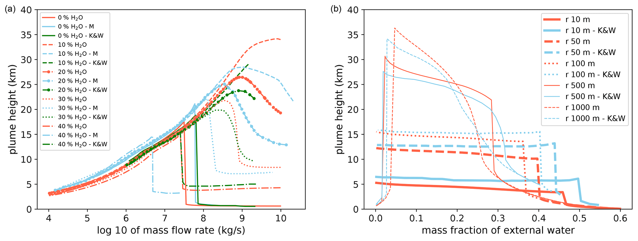
Figure C1 (a) Effect of addition of external water on column height as a function of mass flow rate. As in Koyaguchi and Woods (1996) and Mastin (2007), input parameters are as follows: magma temperature is 1000 K, water vapor mass fraction is 0.03, and relative humidity in the atmosphere is 100 %. The exit velocity for the dry scenario is 100 m s⁻¹, while an adjustment on exit velocities was done for the runs with external water to match the mass flux of magma and gas of the dry case. For this reason, exit velocities are 300, 329, 289, and 236 m s⁻¹ for the runs involving 10 %, 20 %, 30 %, and 40 % of external water, respectively (Mastin, 2007). (b) Plume height as a function of mass fraction of external water added at the vent. Orange lines show the PLUME-MoM-TSM results, while light blue lines are digitized from Fig. 4 of Koyaguchi and Woods (1996). Curves are shown for vent radii of 10, 50, 100, 500, and 100 m. Exit velocity is equal to 100 m s⁻¹, water vapor mass fraction to 0.03, and mixture temperature to 1000 K.

The right panel of Fig. C1 reproduces Fig. 4 of Koyaguchi and Woods (1996), where the height of the eruptive column as a function of the mass of external water added at the vent is shown. Each curve is drawn for a constant mass flow rate of 2.24 ×10⁵, 5.6 ×10⁶, 2.24 ×10⁷, 5.6 ×10⁸, and 2.24 ×10⁹ kg s⁻¹. These values correspond to vent radii of 10, 50, 100, 500, and 1000 m, respectively. The PLUME-MoM-TSM results (orange lines) appear to be similar to those of Koyaguchi and Woods (1996) (light blue lines), although PLUME-MoM-TSM predicts column collapse for slightly lower values of external water than Koyaguchi and Woods (1996). Figures C2 and C3 present the variation of mixture temperature, velocity, relative density, gas mass fraction, and water mass fraction (liquid and ice) as functions of column height for two eruptive scenarios. Each panel shows the results for amounts of external water of 3 (5 in Fig. C3), 10, 20, and 30 wt %. The two figures reproduce Fig. 3 of Koyaguchi and Woods (1996).

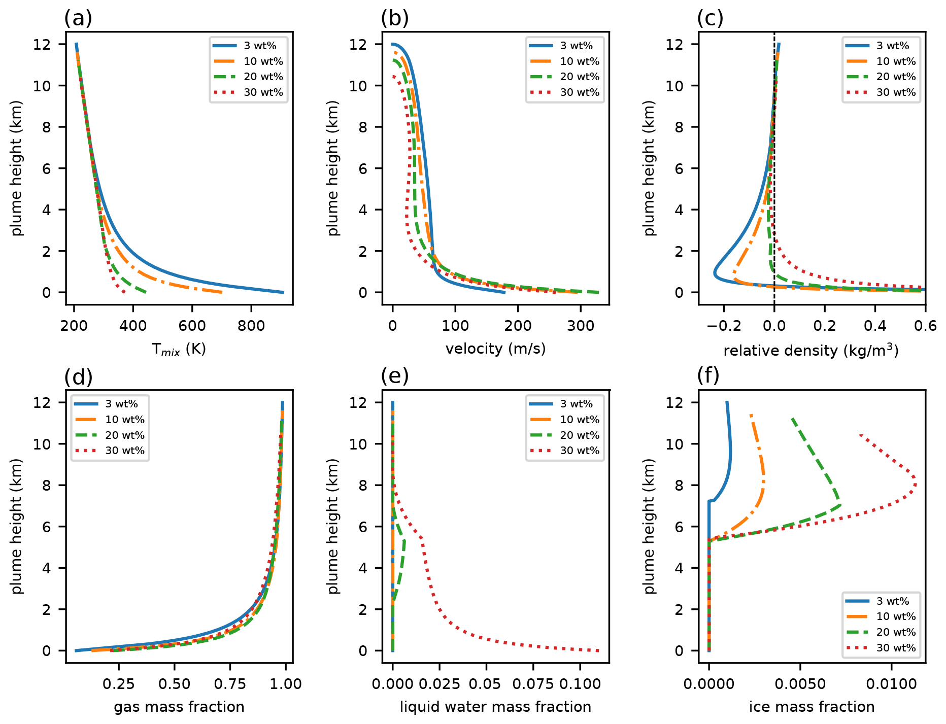
Figure C2 Variation with column height of mixture temperature (a), velocity (b), relative density (c), gas mass fraction (d), liquid mass fraction (e), and ice mass fraction (f). As done in Koyaguchi and Woods (1996), each curve accounts for a different amount of external water added to the magmatic mixture: 3, 10, 20, and 30 wt %. The dry case is set for a vent radius of 50 m and an exit velocity of 100 m s⁻¹, resulting in a mass flow rate of 5.7 ×10⁶ kg s⁻¹. The wet cases are obtained by keeping constant vent radius and mass flow rate, while varying exit velocity. Magma is assumed to contain a 0.03 wt fraction of volatiles (only water vapor) and to have an initial temperature of 1000 K.

Figure C3 As in Fig. C3, but the model is initialized with a vent radius of 1000 m.

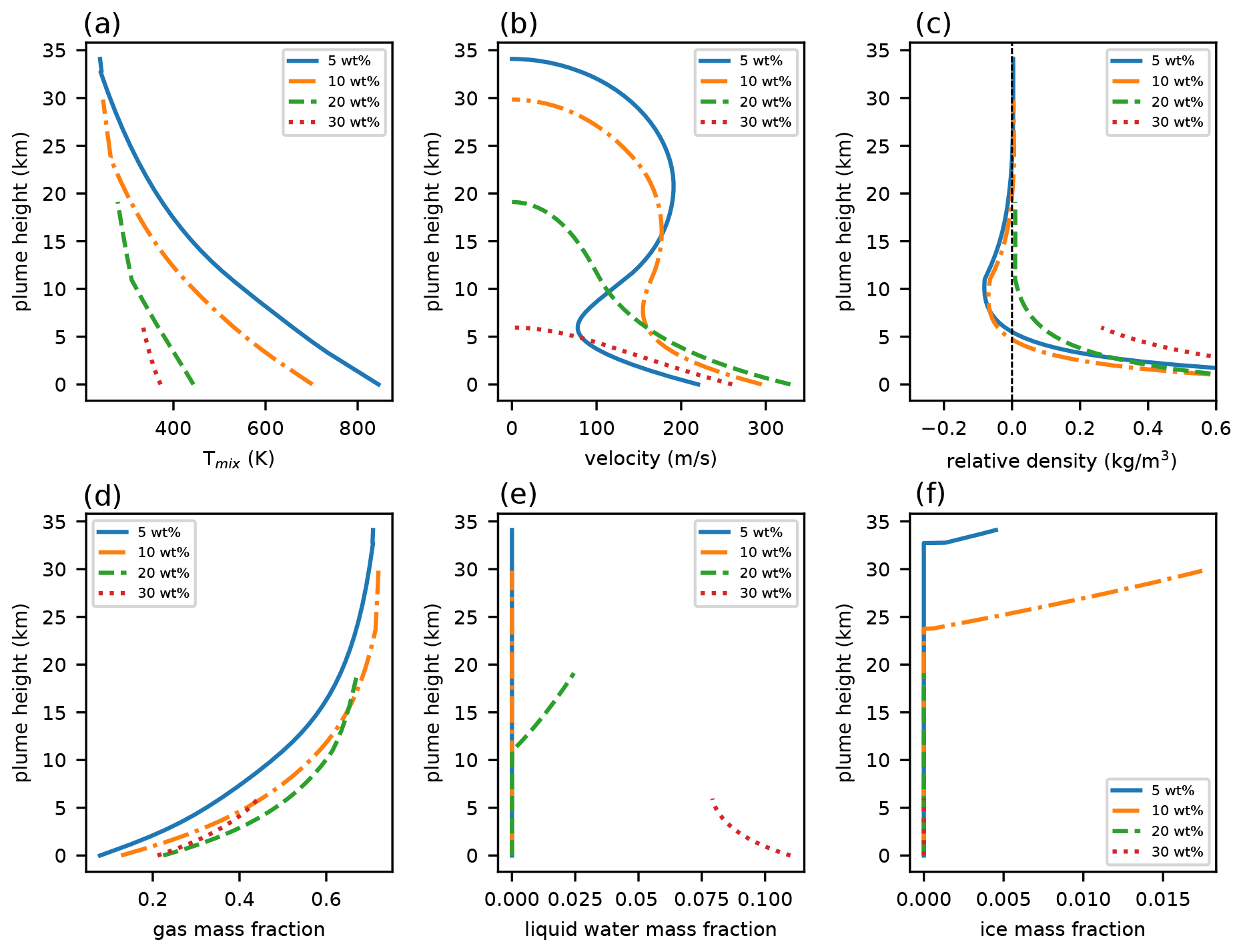
Following Koyaguchi and Woods (1996), Fig. C4 shows the variation of initial mixture density and temperature as the mass of external liquid water increases. The figure shows how the addition of a certain amount of external water alters the properties of the magmatic mixture at the vent. The three curves are done for different initial temperatures of the eruptive mixture (1000 and 1400 K) and volatile contents (0.01 and 0.05 wt fraction; only water vapor is considered). The temperature of the external water is 273 K.

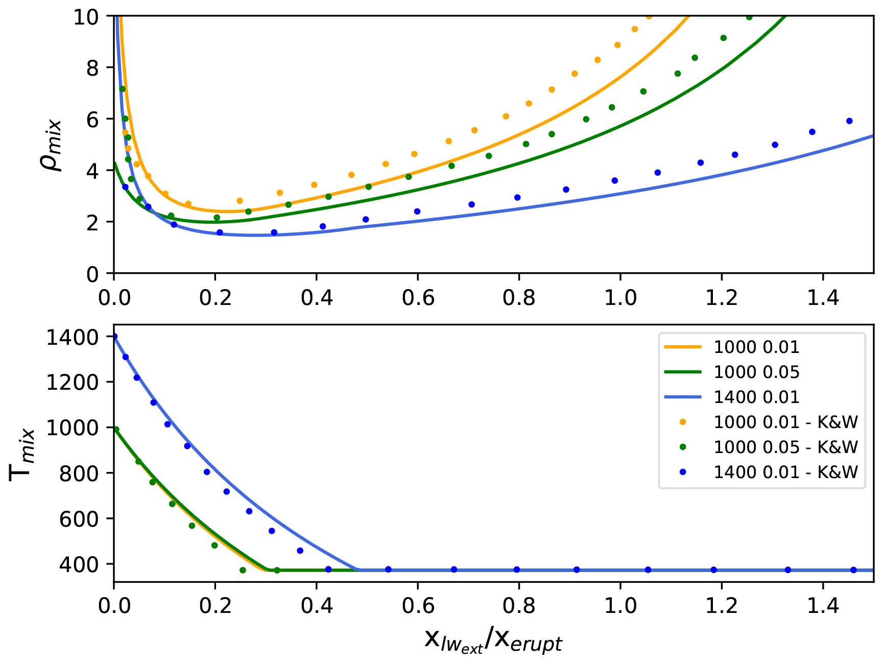
Figure C4 Variation of initial mixture density (ρ_mix) and temperature (T_mix) as the mass of water added to the magma increases. Continuous lines show the results of PLUME-MoM, while dotted lines are digitized from Koyaguchi and Woods (1996). Curves are shown for initial magma temperatures of 1000 and 1400 K, while magma volatile content ranges from 0.01 to 0.05 wt fraction.

Appendix D: List of model variables

Table D1 List of model variables.