the Creative Commons Attribution 4.0 License.
the Creative Commons Attribution 4.0 License.
 | 08 Mar 2021
Using the anomaly forcing Community Land Model (CLM 4.5) for crop yield projections
Xianyu Yang
Crop growth in land surface models normally requires high-temporal-resolution climate data (3-hourly or 6-hourly), but such high-temporal-resolution climate data are not provided by many climate model simulations due to expensive storage, which limits modeling choices if there is an interest in a particular climate simulation that only saved monthly outputs. The Community Land Surface Model (CLM) has proposed an alternative approach for utilizing monthly climate outputs as forcing data since version 4.5, and it is called the anomaly forcing CLM. However, such an approach has never been validated for crop yield projections. In our work, we created anomaly forcing datasets for three climate scenarios (1.5 ∘C warming, 2.0 ∘C warming, and RCP4.5) and validated crop yields against the standard CLM forcing with the same climate scenarios using 3-hourly data. We found that the anomaly forcing CLM could not produce crop yields identical to the standard CLM due to the different submonthly variations, crop yields were underestimated by 5 %–8 % across the three scenarios (1.5, 2.0 ∘C, and RCP4.5) for the global average, and 28 %–41 % of cropland showed significantly different yields. However, the anomaly forcing CLM effectively captured the relative changes between scenarios and over time, as well as regional crop yield variations. We recommend that such an approach be used for qualitative analysis of crop yields when only monthly outputs are available. Our approach can be adopted by other land surface models to expand their capabilities for utilizing monthly climate data.
- Article
(6826 KB) - Full-text XML
-
Supplement
(3347 KB) - BibTeX
- EndNote


Increasing numbers of future climate scenarios exhibit large uncertainties for crop yield projections. Crop yields may increase or decrease depending on which climate projection is used (Lobell et al., 2008; Rosenzweig et al., 2014; Urban et al., 2012). Ensemble future climate projections, such as CMIP5, showed a large range of future climate projections, even for one emission scenario (Knutti and Sedlacek, 2013). Using all future climate projections is not realistic not only because of the computational expense but also because many of these future climate projections only save monthly climate outputs that are not suitable for crop models that require high-temporal-resolution forcing data. Some standalone process-based crop models run in daily time steps, and some crop models embedded in land surface models need at least 6 h of climate data as the forcing data to represent diurnal cycles. Only a small portion of the CMIP5 (Coupled Model Intercomparison Project 5) simulations (< 25 %) can be used as the forcing data for crop models, leaving little room for crop modelers to choose a particular climate model projection that is of interest.
The Community Land Model (CLM) (Oleson et al., 2013) is a state-of-the-art land surface model that simulates biogeophysical (radiation transfer, vegetation-soil-hydrology, surface energy fluxes, etc.) and biogeochemical (soil carbon and nitrogen cycle, vegetation photosynthesis, dynamic vegetation growth, etc.) processes. CLM is the default land model in the Community Earth System Model (CESM) (Hurrell et al., 2013), and it can be run either online coupled with the rest of CESM (atmosphere and ocean) or offline (the land model only, forced with climate datasets) for multiple spatial extents (site, regional, and global) and at different resolutions. The crop model derived from AgroIBIS (Kucharik, 2003) was introduced to CLM4.0 by Levis et al. (2012), and it is responsible for crop growth phenology (temperature determined), carbon allocation algorithms, and crop management (e.g., irrigation). The crop model in CLM runs when the soil biogeochemical component is active, and it was tested with the CLM-CN in version 4.0 and tested with CLM-BGC in version 4.5, where CLM-CN and CLM-BGC are officially supported soil biogeochemical components in CLM4.0 and CLM4.5 respectively. Since their introduction, crop models in the CLM have been developed to represent more crop types and processes, such as soybean nitrogen fixation (Drewniak et al., 2013), ozone impacts on yields (Lombardozzi et al., 2015), winter wheat growth responses to cold hazards (Lu et al., 2017), and maize growth responses to heat stress (Peng et al., 2018). CLM simulates nine crop types, accounting for 54 % of global total crop production (other production is represented by the most similar crop type): maize, soybean, spring wheat, winter wheat, cotton, rice, sugarcane, tropical maize, and tropical soybean. In this study, we used CLM version 4.5 (Oleson et al., 2013).
Since version 4.5, CLM offers a built-in function that indirectly uses monthly climate outputs as the forcing data and is called the anomaly forcing CLM (Lawrence et al., 2015). Anomaly forcing CLM reconstructs new subdaily forcing data by applying the precalculated future monthly anomaly signals to user-defined historical subdaily forcing data, referred to as the reference data. The future monthly anomaly signals are calculated by the future monthly climate outputs and by use of historical monthly outputs. The choice of reference data is arbitrary. Any existing subdaily forcing data (e.g., CRUNCEP, Viovy, 2018, QIAN, Qian et al., 2006) for CLM can be used as the reference data. The historical monthly outputs are recommended to be averaged over multiple years to represent the historical means and avoid affecting the monthly anomaly signal by rare, extreme events in a particular year. Such an arbitrary choice is because the goal of the original anomaly forcing CLM is not to reconstruct future forcing that is identical to the actual future forcing when the high-temporal-resolution data were saved. Rather, the original goal of the anomaly forcing CLM is to understand the influences due to the anomaly signal by comparing the simulation with the anomaly forcing CLM to the simulation run with the reference data. The differences between the two simulations are due to the anomaly signals.
In our study, we modified the anomaly forcing CLM to fit our goals to understand whether we could simply use the anomaly forcing CLM for crop yield projections when only monthly climate data were available. We carefully chose the historical monthly data and the reference data so that the reconstructed future anomaly forcing had nearly identical monthly means to the desired subdaily future forcing, but we used different submonthly variations. We created anomaly forcing datasets for three future scenarios (1.5 ∘C warming, 2.0 ∘C warming, and RCP4.5) for 2006–2075 for which both the subdaily and monthly climate outputs were available from three CESM simulations. With the three paired CLM simulations, we validated the anomaly forcing CLM by comparing it to the standard CLM.
The original anomaly forcing CLM has been available since CLM4.5. This approach reconstructs the subdaily (3-hourly or 6-hourly) forcing data by applying the monthly anomaly signal to user-selected subdaily reference data; therefore, it indirectly uses the monthly atmospheric outputs as the forcing data for CLM. This approach does not change any of the scientific code in CLM; it only adds code that reads the monthly anomaly signals and automatically applies these to the reference data while the CLM is running. There were two monthly anomaly signals for RCP4.5 and RCP8.5 that were generated using the CESM future projections and were ready for use. It is the user's choice to select which subdaily reference (e.g., CRUNCEP or CLMQIAN) and which years to use. By simply modifying the user_nl_cpl name list and adding data streams of the anomaly forcing variables (see the appendix for the detailed usage), the anomaly forcing CLM will automatically read the monthly anomaly signal and apply the signal to each time step of the reference data within a month. When the reference data period is shorter than the anomaly signal period, the anomaly forcing CLM will cycle the same reference data until the simulation is complete. Because the different selections of reference data can generate different forcings, even with the same monthly anomaly signals, one should not use the simulation from the anomaly forcing CLM to represent the actual simulation. Rather, the original goal of the anomaly forcing CLM is to compare the simulation with the anomaly forcing and simulation with the reference forcing data to understand the effects of the monthly anomaly signals on land surface variables.
The goal of this work is to test how well crop yield projections from the anomaly forcing CLM compare to the projections from the standard forcing CLM, given that anomaly forcing has the same monthly average as standard forcing. We selected three future scenarios for CESM simulations that saved both monthly outputs and 3-hourly outputs, where the 3-hourly outputs were directly used in the standard forcing CLM, and the monthly outputs were indirectly used in the anomaly forcing CLM. We calculated the anomaly forcing signals using the monthly CESM outputs and the monthly average of reference data, so that when applying the anomaly signals to the reference data, it is expected to generate identical monthly means as does regular forcing. However, due to a limit in calculations of precipitation anomalies (precipitation anomaly ratio less than 5) and how the CLM treats snow and rainfall, the anomaly forcing CLM did not show identical snow and rainfall monthly averages and introduced bias in the crop yield simulations (see the results section).
Table 1A summary of the original anomaly forcing CLM and the modifications in this work.

We randomly chose the 6-hourly reference data (1996–2005) from one of the 11 historical low-warming ensemble CESM simulations. Additionally, we selected three CESM future simulations for the 1.5 ∘C warming, 2.0 ∘C warming, and RCP4.5 scenarios, where all the three simulations saved both the monthly outputs and the 3-hourly outputs. We then calculated the monthly anomaly signal at each grid cell for each scenario (1.5, 2.0, and RCP45) from 2006–2075. The monthly anomaly signals are differences for temperature, specific humidity, wind, and air pressure and are ratios for solar radiation and precipitation between the monthly outputs of each scenario and the 1996–2005 averaged monthly values of the reference data. The anomaly forcing signal has both spatial and monthly variations. When running the anomaly forcing simulation for 2006–2070, CLM repeatedly uses the 10-year reference period and applies the anomaly signal of a month to all subdaily reference forcing in this month. For example, an anomaly forcing simulation for 2006 January uses the 1996 January reference data plus or multiplied by (if the anomaly signal is a ratio) the 2006 January anomaly signal. If the 2006 January temperature anomaly is 1 K for a grid cell, then all 1996 January reference data will be increased by 1 K for the grid cell.
The monthly anomaly signal is calculated at each grid cell (i,j). For temperature, pressure, wind, and humidity, the anomaly signal is the difference between the future monthly data and the historical monthly average (Eq. 1). For solar radiation, longwave radiation, and precipitation, the anomaly signal is the ratio between the future monthly data and the historical monthly average (Eq. 2). We set the maximum ratio for precipitation to 5 to avoid unrealistic extreme precipitation, which also introduced biases in precipitation (discussed in the discussion section).
Here is anomaly forcing signal at a location i and j in a month m, is the averaged future value, and is the averaged historical value at a location i and j in a month m.
We set up global CLM crop simulations (compset CLM45BGCCROP) at 1.9∘ by 2.5∘ latitude by longitude, respectively, using the anomaly forcing CLM and the regular forcing CLM for the 1.5 ∘C warming, 2.0 ∘C warming, and RCP4.5 scenarios. All simulations used the default nitrogen fertilization rates and a constant CO2 level of 359.8 ppm. For each scenario, we validate the crop yield in the anomaly forcing CLM to the regular forcing CLM to determine if we can use the anomaly forcing CLM for future crop yield projections. We also studied whether the anomaly forcing CLM has a similar crop growth response to transient CO2 and nitrogen fertilization. The transient CO2 and nitrogen fertilization did not add extra computational cost compared to the constant CO2 and nitrogen fertilization simulation. However, due to our limited computational resources we could not afford more experiments, and we only tested such responses for the RCP4.5 scenario. The transient CO2 levels in the RCP45 scenario gradually increased from 379 ppm in 2006 to 530 ppm in 2070. To test the nitrogen fertilization effects, we simply added a zero nitrogen fertilization simulation here. For the crop yield analysis, we aggregated the individual crop yield into an integrated crop yield by area weighted mean based on the crop area map MAPSMAP (https://www.mapspam.info/, last access: 1 March 2021) 2005 crop area. The regional crop yield was simply the regional averaged crop yield at nine regions defined in Ren et al. (2018).
We adopted the two-sample Kolmogorov–Smirnov test (KS test) to test the statistical significance of differences between the anomaly forcing CLM and the standard CLM for atmospheric forcing data and yield. We used the KS test because some variables at some grid cells did not necessarily follow normal distributions. The KS test is a nonparametric test that detects differences in the empirical probability distributions between two samples, and the two samples do not need to have normal distributions (Justel et al., 1997; Marozzi, 2013). When repeated using the 10-year reference data, we expected that the 10-year-averaged monthly anomaly forcing would show no significant differences from the regular forcing. Thus, for the atmospheric forcing data, we tested probability distribution differences between anomaly forcing and regular forcing for every 10-year averaged monthly dataset (sample size was ). For crop yields, we used the every 10-year averaged annual yields (sample size was 7). We used a linear regression coefficient (R2), bias (Eq. 3), and percentage differences (Eq. 4) in our evaluations.
We aimed to generate an anomaly forcing that produced identical monthly averages as its counterpart regular forcing (the desirable 3-hourly forcing data for CLM) but with different submonthly variations. All atmospheric forcing variables achieved this goal except for precipitation and its liquid and ice components, rain and snow. The linear regression coefficients (R2) between anomaly forcing and standard forcing for the monthly means of incoming solar radiation, bottom layer atmosphere temperatures (sigma vertical coordinate, σ=0.9925), pressures, humidities, and winds all showed R2 values above 0.99, and there were also no significant differences for these variables for all grid cells. However, for rain and snow, the R2 values were 0.63–0.87 and 0.88–0.96 across the three scenarios, respectively (Fig. 1a). Statistically significant differences were also found for rain and snow in many regions in the Northern Hemisphere (Fig. 2). We used monthly variances as a measure of the submonthly variations. We calculated the variation for 12 months in each decade, so we have 7 decades and 12 months of variance, and the sample size is 84 when setting up the regression. R2 for variances of forcing were low for most variables except for incoming solar radiation (Fig. 1b). Such lower R2 values indicated that anomaly forcing could not represent the submonthly variations as well as the regular forcing.
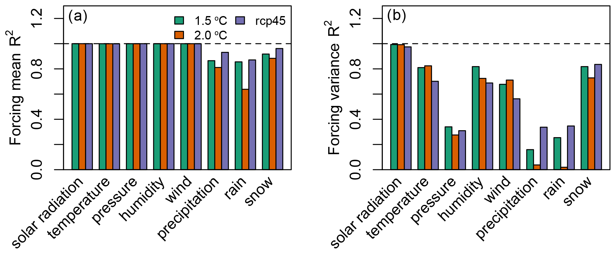
Figure 1Linear regression coefficients (R2) between (a) decade-averaged monthly mean (sample size = 12 months × 7 decades = 84) between anomaly forcing and regular forcing and (b) every 10-year-averaged monthly variance between anomaly forcing and regular forcing.
There were two error sources for precipitation. First, there was overall average lower precipitation in the anomaly forcing by 0.02, 0.03, and 0.2 mm/d in the 1.5, 2.0 ∘C, and RCP45 scenarios, respectively. Such a slightly lower precipitation was because we set the maximum precipitation anomaly ratio to 5 to avoid unrealistically extreme precipitation levels. A ratio of 5 was suggested by NCAR scientists David Lawrence and Sean Swenson, who are core developers of CLM and wrote the initial anomaly forcing code in CLM. Most of the unrealistic extreme precipitation ratios are actually due to the nearly zero historical precipitation (the denominator of Eq. 2). The cap for the precipitation anomaly ratio is used to avoid such situation. Second, the CLM used the temperature in each time step to determine if the given precipitation was rain or snow. Precipitation was rain when temperature was above 273.15 K, otherwise it was snow. Therefore, the different submonthly variations in temperature resulted in different submonthly variations for snow and rain. Due to this problem, the lower precipitation did not evenly distribute to the rain and snow bias, for which rain was underestimated by 0.08–0.3 mm/d, and snow was overestimated by 0.06–0.11 mm/d across the three scenarios. The significantly different regions were mainly in the Northern Hemisphere and the Antarctic, and most regions in the Southern Hemisphere did not show significant differences in rain or snow. How the rain and snow biases affected yield projections will be discussed.
When compared to crop yield simulations in the standard CLM, the anomaly forcing CLM underestimated crop yields by 5 %–8 % across the three scenarios for the global average, and 28 %–41 % of cropland showed statistically significant differences in yields. The rainfed crop yield differences across the three scenarios showed largely similar spatial distributions: overestimation in the northern US and Europe and underestimation in the Southern Hemisphere and in East Asia (Fig. 3d–f). The overestimated rainfed crop yield (mainly for maize and wheat) in the anomaly forcing CLM is due to higher water availability in these regions, which is a result of higher snow in the anomaly forcing CLM. For irrigated crops, such overestimations in the northern US and Europe disappear (Fig. 3g–i) because sufficient irrigation was added to the irrigated soil column in the standard CLM, which removed the plant water stress that was seen for rainfed crops. However, the underestimations in the Southern Hemisphere and East Asia were persistent, because water availability does not cause yield differences for irrigated crops; we suspect such underestimations were caused by the other error in forcing data: the different submonthly variations in the forcing data.
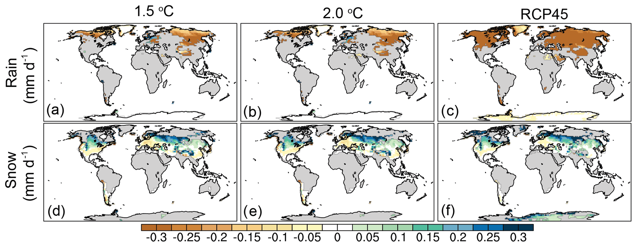
Figure 270-year averaged differences between anomaly forcing and regular forcing for rain (a–c) and snow (d–f) for the 1.5, 2.0 ∘C, and RCP4.5 scenarios. All differences shown here are statistically significant differences tested using the Kolmogorov–Smirnov test with a sample size of 84. The gray areas are regions that did not show significant differences.
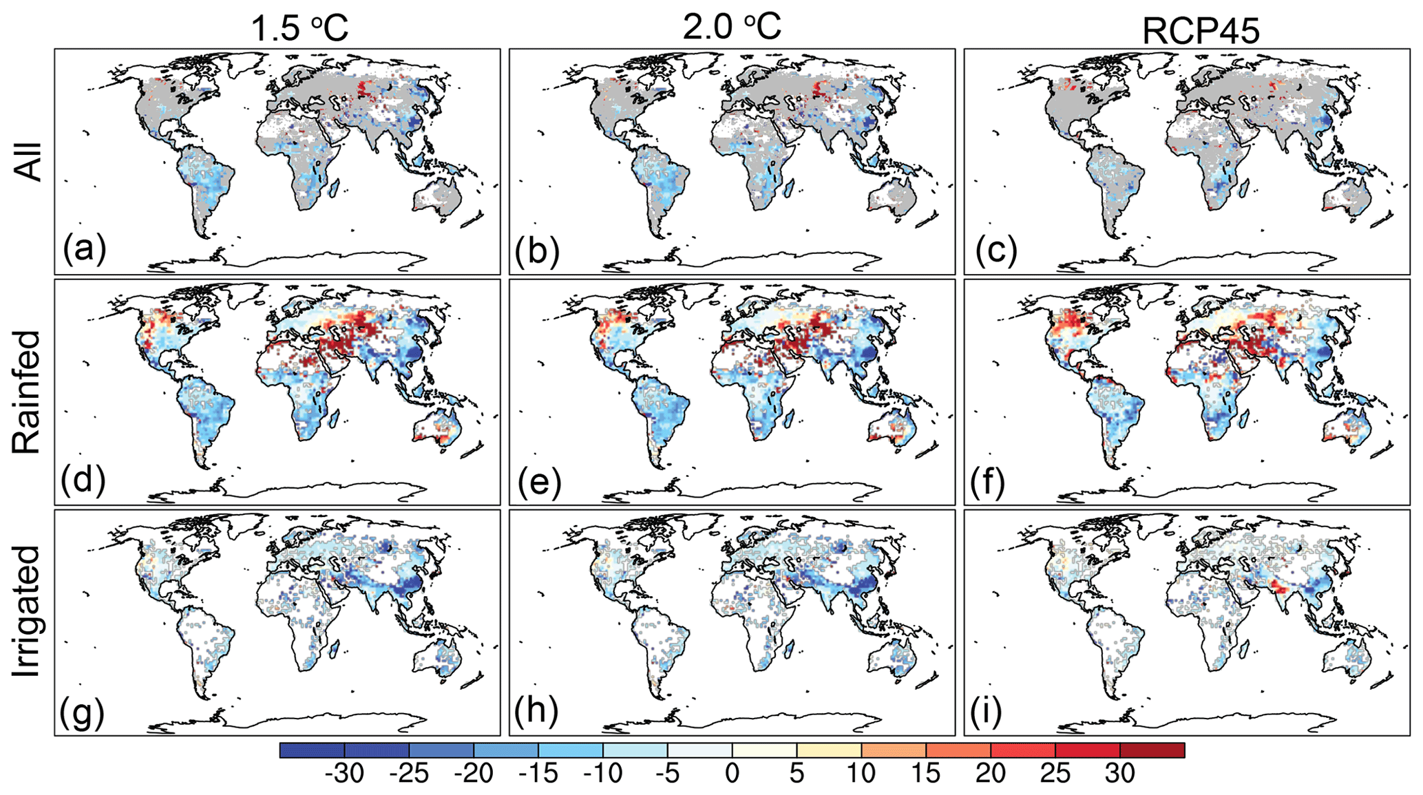
Figure 3The percentage differences of 70-year integrated yields between the anomaly forcing CLM and the standard CLM for all crops (a–c), rainfed crops (d–f), and irrigated crops (g–i) for the 1.5, 2.0 ∘C, and RCP45 scenarios. The white regions are where no crops grow based on the historical crop map in 2005 (MAPSPAM 2005; https://www.mapspam.info/, last access: 1 March 2021). For plots (a)–(c), we showed only the significant differences as determined using the Kolmogorov–Smirnov test with a sample size of 7. The regions with insignificant differences are masked as gray in (a)–(c). For plots (d)–(i), we did not mask the insignificant differences to show an overall bias.
The global 70-year averaged yields ± standard deviation in the standard CLM (Ren et al., 2018) and in the anomaly forcing CLM are 4.38 ± 0.09 and 4.03 ± 0.16 t/ha, respectively, in the 1.5 ∘C scenario; 4.36 ± 0.11 and 4.01 ± 0.14 t/ha, respectively, in the 2.0 ∘C scenario; and 3.95 ± 0.13 and 3.72 ± 0.14, respectively, in the RCP45 scenario (Fig. 4). The anomaly forcing CLM captured the regional yield variations. Latin America (LAC) showed the highest yield while India (IND) showed the lowest yields for both the anomaly forcing CLM and the standard CLM across the three scenarios.
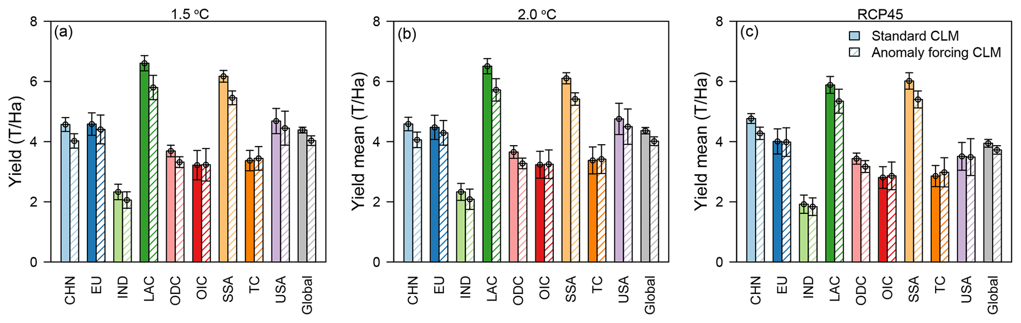
Figure 4Regional comparisons of the 70-year integrated mean yields and yield standard deviations between the anomaly forcing CLM and the standard CLM. The error bars indicate 70-year yield standard deviations. CHN: China; EU: European Union; IND: India; LAC: Latin America; ODC: other developing countries; OIC: other industrialized countries; SSA: sub-Saharan Africa; TC: transition countries; USA: United States.
Although the crop yields were underestimated, the anomaly forcing CLM could qualitatively represent the spatial yield differences between two climate scenarios. Comparing 2.0 to 1.5 ∘C, there was a 4 %–8 % yield increase in the northern US and a 0 %–4 % yield decrease (Fig. 5a) in the southeastern US. When comparing the RCP45 to the 1.5 ∘C scenario, crop yields in the US were largely reduced (up to 50 %). The anomaly forcing CLM clearly captured these yield differences (Fig. 5b and d).
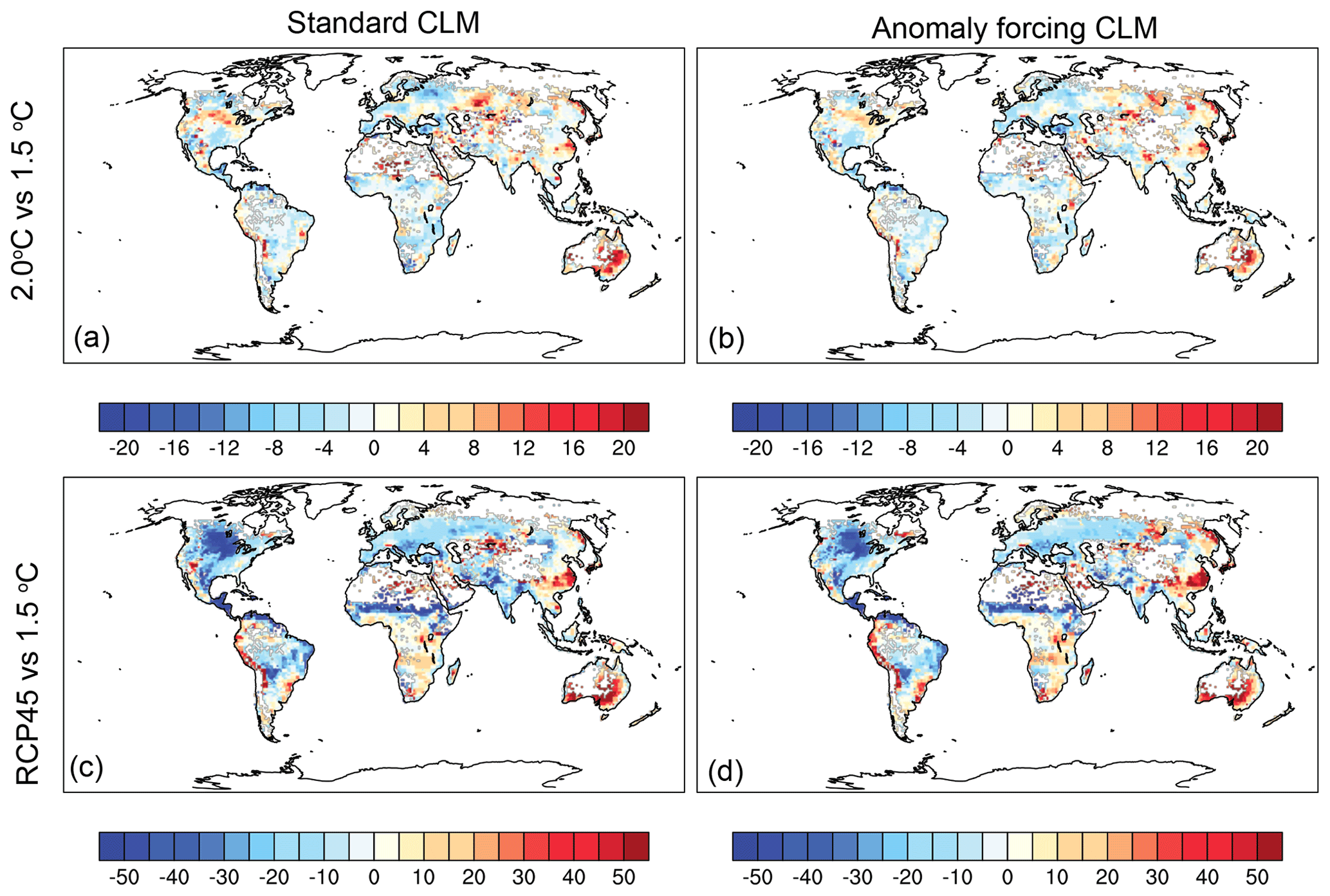
Figure 5The percentage of 70-year integrated yield differences between 2.0 and 1.5 ∘C (a, b) and between RCP45 and 1.5 (c, d) in the standard CLM and the anomaly forcing CLM.
The anomaly forcing CLM also captured yield changes over time for each climate scenario. The three scenarios showed some similarities in yield changes from 2006–2015 to 2066–2075. For example, crop yields increased in southeastern China and decreased in sub-Saharan Africa. There were also yield changes that were unique to each scenario that were also found in the anomaly forcing CLM. For example, crop yields increased in Europe for the 1.5 ∘C scenario (Fig. 6a–b) while they decreased in Europe for the 2.0 ∘C and RCP45 scenarios (Fig. 6c–f), and crop yields declined in the US for the RCP45 scenario (Fig. 6e–f) while they increased for the 1.5 and 2.0 ∘C scenarios (Fig. 6a–d).
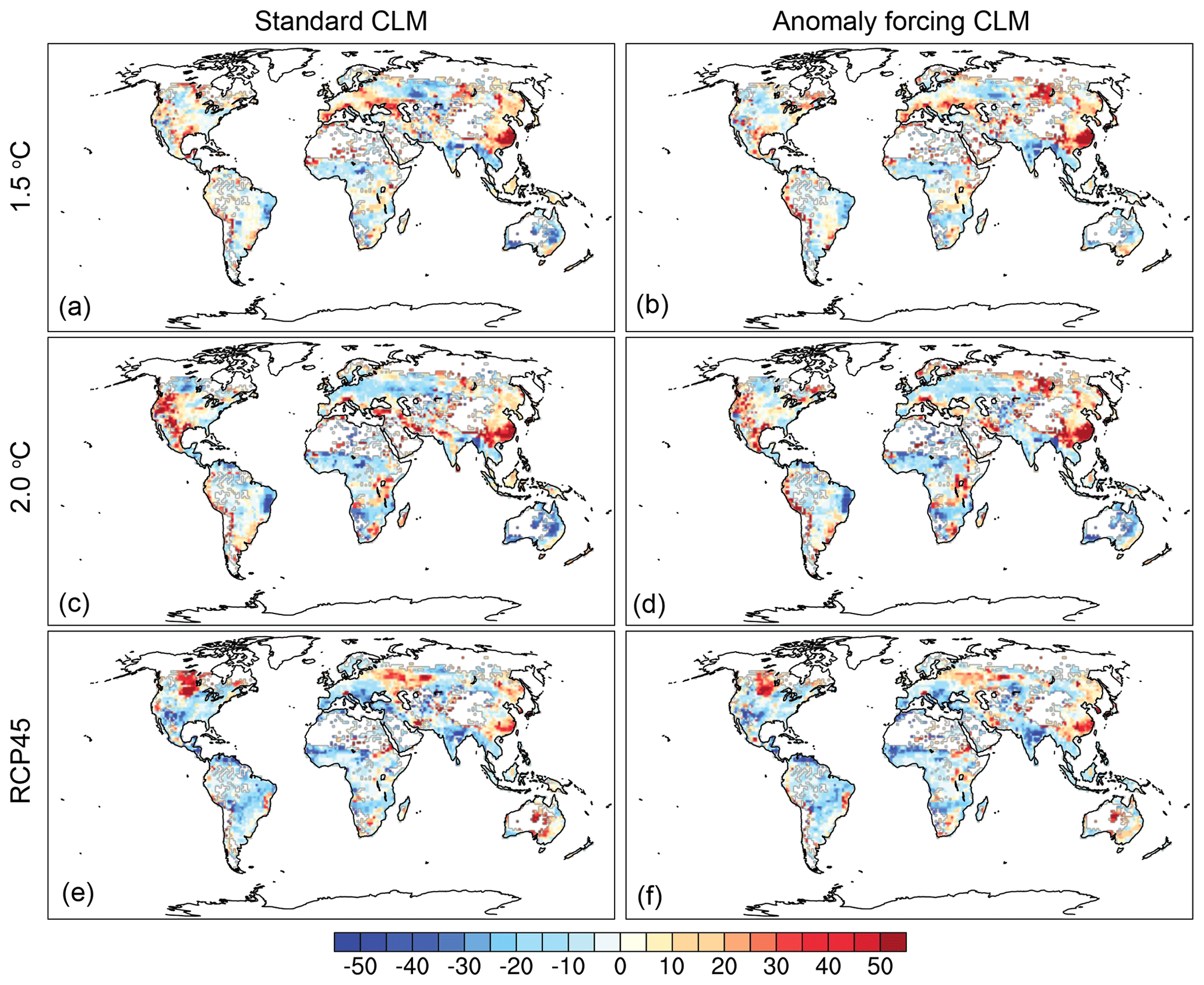
Figure 6The percentage yield difference from 2006–2015 to 2066–2075 in the standard CLM and anomaly forcing CLM across the three scenarios.
All simulations in the above evaluations adopted a constant CO2 level (359.8 ppm) and crop-type-dependent fixed nitrogen fertilization (25–500 kgN/ha), so whether the anomaly forcing CLM simulated a similar or different crop growth response to CO2 or nitrogen fertilization is unknown. Due to limited computational resources, we tested crop responses to transient CO2 and nitrogen fertilization only for the RCP45 scenario and assumed that the other scenarios would show the same differences as the RCP45 scenario. The transient CO2 in the RCP45 scenario gradually increased from 379 ppm in 2006 to 530 ppm in 2075. To test the effects of nitrogen fertilization, we simply added a zero nitrogen fertilization simulation. Although all grid cells had the same amounts of CO2 increase in a given year (no spatial variation), crop yields had spatial variations in response to transient CO2. Most regions showed a 5 %–10 % yield increase, but some regions showed much higher yield increases, such as northern India, the southern edge of the Sahara, and Australia (Fig. 7a). Such crop yield responses to transient CO2 spatial patterns were also captured by the anomaly forcing CLM (Fig. 7b). Similar for the crop yield responses to nitrogen fertilization, the anomaly forcing CLM simulated crop yield increase spatial patterns (Fig. 7c–d), in which the Southern Hemisphere and Asia had greater yield increases in response to nitrogen fertilization.
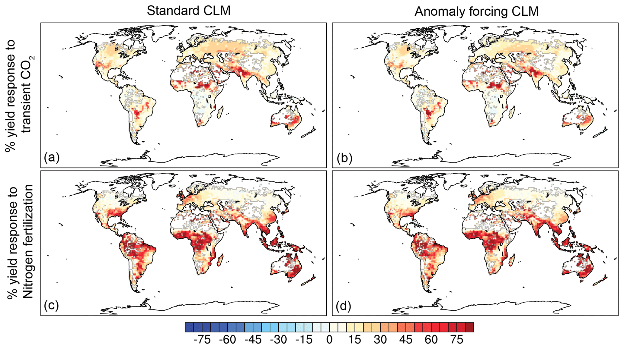
Figure 770-year averaged integrated crop yield response to transient CO2 and to no nitrogen fertilization in the anomaly forcing CLM (a, b) and in the standard CLM (c, d) for the RCP45 scenario.
In this work, we created anomaly forcing datasets for three future climate scenarios, and we validated the crop yields in the anomaly forcing CLM by comparison with the crop yields in the standard CLM. The differences between the anomaly forcing CLM and standard CLM were due only to differences in forcing data, for which the standard CLM used regular forcing (3-hourly forcing) and the anomaly forcing CLM used anomaly forcing. We found that the anomaly forcing CLM underestimated crop yields but identified the regional yield variations, as well as yield differences between two climate scenarios and yield changes over time. The anomaly forcing CLM could not generate the exact same crop yields as the standard CLM due to errors in precipitation and in the submonthly variations. However, it could be used for qualitative analysis of relative crop yield changes among different scenarios and over time.
The overall underestimation of crop yields may be due to differences in phenology that resulted from different submonthly variations. Some of the low yields in the anomaly forcing CLM may be explained by shorter grain fill periods. For example, the lower rice yields in southeastern China are due to a 5–10 d shorter grain fill period in the anomaly forcing CLM (Fig. S1a–c in the Supplement); maize and soybean in the Southern Hemisphere also showed a 1–5 d shorter grain fill period that may account for the lower yields (Fig. S1d–i). In addition to the low yields, the anomaly forcing CLM also simulated lower GPP and LAI compared to the standard CLM (Fig. S2a1–b3), and the spatial distributions of GPP and LAI differences were very similar to the yield differences.
Some regions in the Northern Hemisphere showed higher rainfed crop yields in the anomaly forcing CLM, which is due to higher soil moisture at planting that resulted from higher snow levels in the Northern Hemisphere. Crop growth in CLM is very sensitive to the soil moisture at planting, and higher soil moisture (Fig. S2c1–c3) results in unstressed crop growth and hence produces higher yields. When adequate irrigation is applied, both the anomaly forcing and the standard CLM models have sufficient water for crop growth, and the overestimations disappeared. Therefore, the anomaly forcing may not be appropriate for estimating the actual future irrigation demands but is able to distinguish the relative differences in irrigation demand across different climate scenarios.
The energy fluxes in the anomaly forcing CLM and in the standard CLM were different due to different crop growth rates and differences in forcing data. The higher snow cover in the Northern Hemisphere creates higher albedo and lower absorbed solar radiation and hence lower surface energy fluxes. The higher LAI increased the summer latent heat flux up to 5 W/m2 (Fig. S3), while the annual latent heat flux showed values 5–10 W/m2 (Fig. S2d1–d3) lower in the anomaly forcing CLM due to the lower net radiation. In the Southern Hemisphere, lower LAI (Fig. S2a1–a3) resulted in lower latent heat fluxes (Fig. S2d1–d3) and higher sensible heat fluxes (Fig. S2e1–e3).
The regional yield comparisons indicate that the anomaly forcing CLM effectively captured regional yield variations but with slightly lower yield biases. We want to point out that the very high crop yields in Latin America and sub-Saharan Africa and the very low crop yields in India in both the anomaly forcing CLM and the standard CLM approaches are not realistic when compared to the UNFAO yields (http://www.fao.org/statistics/en/, last access: 1 March 2021). Such biases in the CLM have been discussed by Levis et al. (2018), and the low yields in India are due to incorrect crop phenology when crops entered the grain fill during the dry season. The high yields in Latin American and in sub-Saharan Africa were due to the nitrogen fertilization amounts based on US levels, which are too high for these regions.
The crop model in the most recent version of CLM5.0 includes new features as reported in Lombardozzi et al. (2020). For example CLM5.0 uses time-varying spatial distributions of major crop types and has updated fertilization and irrigation schemes. These updates of crop model in CLM5.0 may improve the crop yield simulations for both standard CLM and anomaly forcing CLM compared to crop yield in reality. The anomaly forcing method in CLM5.0 remains unchanged so we speculate that the bias due to anomaly forcing may still exist in CLM5.0. For example, CLM5.0 uses the same threshold to differentiate rain and snow, so the bias due to higher snow cover in the Northern Hemisphere may still exist in CLM5.0. However, how the magnitude of the bias will change is unclear. We suggest that the anomaly forcing of CLM5.0 be tested if the research interest is in absolute yield or in qualitative difference.
Our approach can be adopted by other land surface models to expand their capabilities for utilizing monthly climate data. The source code of the anomaly forcing CLM is available at the repository website Zenodo https://doi.org/10.5281/zenodo.3900671 (Lu, 2020). The path is post4.5crop_slevis/models/lnd/clm/src/cpl/lnd_import_ export.F90 when unzip post4.5crop_slevis_codeforGMD.tar.gz. The Fortran code could be transplanted to other land surface models which use NetCDF format atmospheric forcing.
The Community Land Surface model offers an alternative way to utilize the monthly climate as the forcing data. Such an approach could expand user choice of forcing data when high-temporal-resolution climate data are not available. In this work, we created anomaly forcing data for three climate scenarios (1.5 ∘C warming, 2.0 ∘C warming, and RCP4.5) and validated crop yield projections in the anomaly forcing CLM against the standard CLM. The anomaly forcing CLM underestimated crop yields by 5 %–8 %, which was largely due to the differences in phenology and photosynthesis that resulted from the different submonthly variations. How CLM treated precipitation as rain or snow also introduced biases in crop yields and in the energy flux simulations. Although the anomaly forcing CLM could not generate crop yields identical to the standard CLM, it could be used for qualitative analysis of crop yield changes across various scenarios over time.
Running the anomaly forcing CLM is similar to the standard CLM but with several additional steps. First, the monthly anomaly data are prepared as described in the method section. Then, the user needs to modify user_nl_cpl and user_nl_datm to specify which forcing variables to add to the anomaly signals. There are seven anomaly forcing variables (Table A2), and the user can specify one, or two, or all variables in the two name lists (user_nl_cpl and user_nl_datm). The final step is to add the corresponding anomaly forcing data streams depending on which anomaly forcing variables were specified in user_nl_cpl and user_nl_datm.
A1 Modify user_nl_cpl and user_nl_datm
The user may add part or all of the following text to user_nl_ cpl.
cplflds_custom = 'Sa_prec_af->a2x',
'Sa_prec_af->x2l','Sa_tbot_af->a2x',
'Sa_tbot_af->x2l','Sa_pbot_af->a2x',
'Sa_pbot_af->x2l','Sa_shum_af->a2x',
'Sa_shum_af->x2l','Sa_u_af->a2x',
'Sa_u_af->x2l','Sa_v_af->a2x',
'Sa_v_af-> x2l','Sa_swdn_af->a2x',
'Sa_swdn_af->x2l','Sa_lwdn_af-> a2x',
'Sa_lwdn_af->x2l'
Add part or all of the following text into user_nl_datm.
anomaly_forcing= 'Anomaly.Forcing.Precip',
'Anomaly.Forcing.Temperature', 'Anomaly.Forcing.Pressure', 'Anomaly.Forcing.Humidity',
'Anomaly.Forcing.Uwind', 'Anomaly.Forcing.Vwind',
'Anomaly.Forcing.Shortwave', 'Anomaly.Forcing.Longwave'
Also attach the anomaly forcing data streams in user_nl_datm.
streams = “datm.streams.txt.CLMCRUNCEP.Solar 1996 1996 2005”, “datm.streams.txt.CLMCRUNCEP.Precip 1996 1996 2005”,
“datm.streams.txt.CLMCRUNCEP.TPQW 1996 1996 2005”,
“datm.streams.txt.presaero.clim_2000 1 1 1”,
“datm.streams.txt.Anomaly.Forcing.Precip 2006 2006 2075”,
“datm.streams.txt.Anomaly.Forcing.Temperature 2006 2006 2075”,
“datm.streams.txt.Anomaly.Forcing.Pressure 2006 2006 2075”,
“datm.streams.txt.Anomaly.Forcing.Humidity 2006 2006 2075”,
“datm.streams.txt.Anomaly.Forcing.Uwind 2006 2006 2075”,
“datm.streams.txt.Anomaly.Forcing.Vwind 2006 2006 2075”,
“datm.streams.txt.Anomaly.Forcing.Shortwave 2006 2006 2075”,
“datm.streams.txt.Anomaly.Forcing.Longwave 2006 2006 2075”,
“/glade/p/work/yaqiong/inputdata/atm/datm7/co2.1pt5degC. streams.txt 1901 1901 2075”
mapalgo = 'bilinear', 'bilinear', 'bilinear', 'bilinear', 'bilinear', 'bilinear', 'bilinear', 'bilinear', 'bilinear',
'bilinear', 'bilinear', 'bilinear','nn'
tintalgo = 'coszen', 'nearest', 'linear', 'linear', 'nearest', 'nearest', 'nearest', 'nearest', 'nearest', 'nearest',
'nearest', 'nearest','linear'
Any combination or subset of anomaly forcing variables can be used. For example,
cplflds_custom = 'Sa_prec_af->a2x', 'Sa_ prec_af->x2l' (in user_nl_cpl)
anomaly_forcing='Anomaly.Forcing.Precip' (in user_nl_datm)
will only adjust precipitation. The reference data and period are defined in env_run.xml.
A2 Add the anomaly forcing data stream
The anomaly forcing data stream is where the data path of the monthly anomaly forcing signal can be specified and the code can be told which variable to retrieve. A list of all anomaly forcing data stream file names and the variables in the anomaly forcing data and the code are given in Table A1. An example of the content in user_datm.streams.txt.Anomaly.Forcing.Humidity is also attached. The user only needs to add the corresponding variable data streams that are defined in user_nl_cpl.
Table A1A list of the anomaly forcing data streams and the corresponding variables in the anomaly forcing data and the code.
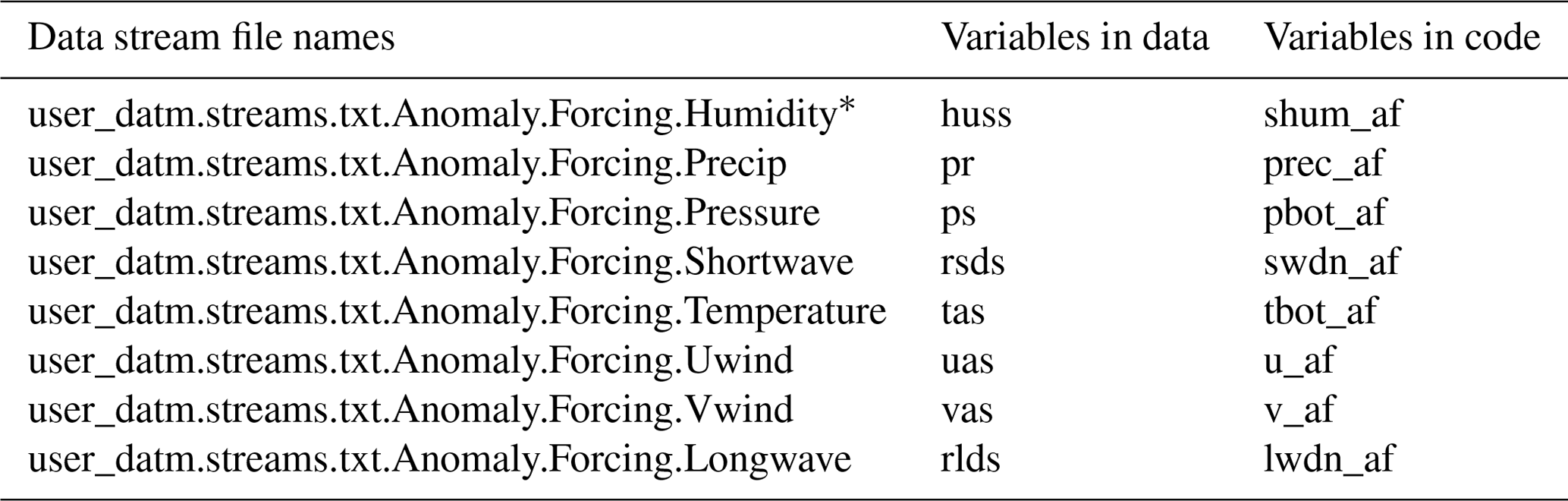
* An example of the content in the data stream is given below.
< dataSource>
GENERIC
< /dataSource>
< domainInfo>
< variableNames>
time
xc lon
yc lat
area
mask
< /variableNames>
< filePath>
/glade/p/cesmdata/cseg/inputdata/share/domains
< /filePath>
< fileNames>
domain.lnd.fv0.9x1.25_gx1v6.090309.nc
< /fileNames>
< /domainInfo>
< fieldInfo>
< variableNames>
huss shum_af
< /variableNames>
< filePath>
THE ANOMALY FORCING SIGNAL DATA PATH
< /filePath>
< fileNames>
THE ANOMALY FORCING SIGNAL DATA NAME
< /fileNames>
< offset>
0
< /offset>
< /fieldInfo>
The CLM source code used in our study is available at repository website Zenodo: https://doi.org/10.5281/zenodo.3900671 (Lu, 2020).
Our research data are available at the repository website Zenodo at https://doi.org/10.5281/zenodo.4571653 (Lu, 2021).
The supplement related to this article is available online at: https://doi.org/10.5194/gmd-14-1253-2021-supplement.
YL designed and performed the simulations. YL and XY analyzed the results and wrote the paper.
The authors declare that they have no conflict of interest.
We thank the topical editor Christoph Müller and two anonymous reviewers for their great comments that largely improved our paper. We also thank NCAR scientists Sean Swenson and David Lawrence for the instruction of using the anomaly forcing approach, and Peter Lawrence for providing the crop area maps. This work was supported by the National Science Foundation under grant number AGS-1243095 and the National Natural Science Foundation of China (no. 41975135). We would like to acknowledge high-performance computing support from Yellowstone (ark:/85065/d7wd3xhc), provided by NCAR's Computational and Information Systems Laboratory, sponsored by the National Science Foundation.
This research has been supported by the National Science Foundation (grant no. AGS-1243095) and the National Natural Science Foundation of China (grant no. 41975135).
This paper was edited by Christoph Müller and reviewed by two anonymous referees.
Drewniak, B., Song, J., Prell, J., Kotamarthi, V. R., and Jacob, R.: Modeling agriculture in the Community Land Model, Geosci. Model Dev., 6, 495–515, https://doi.org/10.5194/gmd-6-495-2013, 2013.
Hurrell, J. W., Holland, M. M., Gent, P. R., Ghan, S., Kay, J. E., Kushner, P. J., Lamarque, J. F., Large, W. G., Lawrence, D., Lindsay, K., Lipscomb, W. H., Long, M. C., Mahowald, N., Marsh, D. R., Neale, R. B., Rasch, P., Vavrus, S., Vertenstein, M., Bader, D., Collins, W. D., Hack, J. J., Kiehl, J., and Marshall, S.: The Community Earth System Model A Framework for Collaborative Research, B. Am. Meteorol. Soc., 94, 1339–1360, 2013.
Justel, A., Pena, D., and Zamar, R.: A multivariate Kolmogorov-Smirnov test of goodness of fit, Stat. Probabil. Lett., 35, 251–259, 1997.
Knutti, R. and Sedlacek, J.: Robustness and uncertainties in the new CMIP5 climate model projections, Nat. Clim. Change, 3, 369–373, 2013.
Kucharik, C. J.: Evaluation of a Process-Based Agro-Ecosystem Model (Agro-IBIS) across the US Corn Belt: Simulations of the Interannual Variability in Maize Yield, in: Earth Interact, 7, 14, 2003.
Lawrence, D. M., Koven, C. D., Swenson, S. C., Riley, W. J., and Slater, A. G.: Permafrost thaw and resulting soil moisture changes regulate projected high-latitude CO2 and CH4 emissions, Environ. Res. Lett., 10, 094011, https://doi.org/10.1088/1748-9326/10/9/094011, 2015.
Levis, S., Badger, A., Drewniak, B., Nevison, C., and Ren, X. L.: CLMcrop yields and water requirements: avoided impacts by choosing RCP 4.5 over 8.5, Climatic Change, 146, 501–515, 2018.
Levis, S., Bonan, G. B., Kluzek, E., Thornton, P. E., Jones, A., Sacks, W. J., and Kucharik, C. J.: Interactive Crop Management in the Community Earth System Model (CESM1): Seasonal Influences on Land-Atmosphere Fluxes, J. Climate, 25, 4839–4859, 2012.
Lobell, D. B., Burke, M. B., Tebaldi, C., Mastrandrea, M. D., Falcon, W. P., and Naylor, R. L.: Prioritizing climate change adaptation needs for food security in 2030, Science, 319, 607–610, 2008.
Lombardozzi, D., Levis, S., Bonan, G., Hess, P. G., and Sparks, J. P.: The Influence of Chronic Ozone Exposure on Global Carbon and Water Cycles, J. Climate, 28, 292–305, 2015.
Lombardozzi, D. L., Lu, Y. Q., Lawrence, P. J., Lawrence, D. M., Swenson, S., Oleson, K. W., Wieder, W. R., and Ainsworth, E. A.: Simulating Agriculture in the Community Land Model Version 5, J. Geophys. Res.-Biogeo., 125, e2019JG005529, https://doi.org/10.1029/2019JG005529, 2020.
Lu, Y., Williams, I. N., Bagley, J. E., Torn, M. S., and Kueppers, L. M.: Representing winter wheat in the Community Land Model (version 4.5), Geosci. Model Dev., 10, 1873–1888, https://doi.org/10.5194/gmd-10-1873-2017, 2017.
Lu, Y.: Source code for Using the anomaly forcing Community Land Model (CLM) for crop yield projections, Zenodo, https://doi.org/10.5281/zenodo.3900671, 2020.
Lu, Y.: Crop yield data of Using the anomaly forcing Community Land Model (CLM 4.5) for crop yield projections, Zenodo, https://doi.org/10.5281/zenodo.4571653, 2021.
Marozzi, M.: Nonparametric Simultaneous Tests for Location and Scale Testing: A Comparison of Several Methods, Commun. Stat.-Simul. C, 42, 1298–1317, 2013.
Oleson, K., Lawrence, D., Bonan, G., Drewniak, B., Huang, M., Koven, C., Levis, S., Li, F., Riley, W., Subin, Z., Swenson, S., and Thornton, P.: Technical Description of version 4.5 of the Community Land Model (CLM), National Center for Atmospheric Rsearch, Boulder, CO, NCAR/TN-503+STR, 434 pp., 2013.
Peng, B., Guan, K. Y., Chen, M., Lawrence, D. M., Pokhrel, Y., Suyker, A., Arkebauer, T., and Lu, Y. Q.: Improving maize growth processes in the community land model: Implementation and evaluation, Agr. Forest. Meteorol., 250, 64–89, 2018.
Qian, T., Dai, A., Ternberth, K. E., and Olseon, K. W.: Simulation of Global Land Surface Conditions from 1948 to 2004. Part I: Forcing Data and Evaluations, J. Hydrometeorol., 7, 953–975, 2006.
Ren, X., Lu, Y., O'Neill, B. C., and Weitzel, M.: Economic and biophysical impacts on agriculture under 1.5 ∘C and 2 ∘C warming, Environ. Res. Lett., 13, 115006, https://doi.org/10.1088/1748-9326/aae6a9, 2018.
Rosenzweig, C., Elliott, J., Deryng, D., Ruane, A. C., Muller, C., Arneth, A., Boote, K. J., Folberth, C., Glotter, M., Khabarov, N., Neumann, K., Piontek, F., Pugh, T. A. M., Schmid, E., Stehfest, E., Yang, H., and Jones, J. W.: Assessing agricultural risks of climate change in the 21st century in a global gridded crop model intercomparison, P. Natl. Acad. Sci. USA, 111, 3268–3273, 2014.
Urban, D., Roberts, M. J., Schlenker, W., and Lobell, D. B.: Projected temperature changes indicate significant increase in interannual variability of U.S. maize yields, Climatic Change, 112, 525–533, 2012.
Viovy, N.: CRUNCEP Version 7 – Atmospheric Forcing Data for the Community Land Model, Research Data Archive at the National Center for Atmospheric Research, Computational and Information Systems Laboratory, https://doi.org/10.5065/PZ8F-F017, 2018.