the Creative Commons Attribution 4.0 License.
the Creative Commons Attribution 4.0 License.
 | 08 Mar 2021
On the model uncertainties in Bayesian source reconstruction using an ensemble of weather predictions, the emission inverse modelling system FREAR v1.0, and the Lagrangian transport and dispersion model Flexpart v9.0.2
Pieter De Meutter
Ian Hoffman
Kurt Ungar
Bayesian source reconstruction is a powerful tool for determining atmospheric releases. It can be used, amongst other applications, to identify a point source releasing radioactive particles into the atmosphere. This is relevant for applications such as emergency response in case of a nuclear accident or Comprehensive Nuclear-Test-Ban treaty verification. The method involves solving an inverse problem using environmental radioactivity observations and atmospheric transport models. The Bayesian approach has the advantage of providing an uncertainty quantification on the inferred source parameters. However, it requires the specification of the inference input errors, such as the observation error and model error. The latter is particularly hard to provide as there is no straightforward way to determine the atmospheric transport and dispersion model error. Here, the importance of model error is illustrated for Bayesian source reconstruction using a recent and unique case where radionuclides were detected on several continents. A numerical weather prediction ensemble is used to create an ensemble of atmospheric transport and dispersion simulations, and a method is proposed to determine the model error.
- Article
(3945 KB) - Full-text XML
-
Supplement
(2307 KB) - BibTeX
- EndNote


Nuclear facilities release a certain amount of anthropogenic radioactive particulates or gases into the atmosphere, which are transported and dispersed by the wind. These releases can either be routine or accidental. Several countries run a network of stations to monitor airborne levels of environmental radioactivity (Steinhauser, 2018). These monitoring networks allow the verification of compliance with regulatory release limits but also the detection of reported and unreported nuclear events. Recent examples include the detections of 131I in Europe (Masson et al., 2018) or 106Ru detections on the Northern Hemisphere (Masson et al., 2019).
On the international scale, the radionuclide component of the International Monitoring System will consist of 80 stations measuring radioactive particulates (of which at least 40 will be equipped with radioactive noble gas detectors). This network is being set up to verify compliance with the Comprehensive Nuclear-Test-Ban Treaty once it enters into force. In the past, anomalous radionuclide detections were made that are likely linked to a nuclear explosion (Ringbom et al., 2014; De Meutter et al., 2018).
If an anomalous1 detection occurred (either from a nuclear accident or a clandestine nuclear weapon test), methods are needed that relate the detection with its source or potential sources if the source is unknown. One of these methods is atmospheric transport and dispersion modelling. An atmospheric transport and dispersion model typically simulates the transport, dispersion, dry and wet deposition, and radioactive decay of radionuclides released in the atmosphere. These processes establish a linear relationship between the concentrations at receptors and the release amount at the source. One can calculate such source–receptor relationships (Seibert and Frank, 2004) between a fixed source and several receptors or stations (when modelling forward in time) or between a fixed receptor and several potential sources (when modelling backwards in time).
A significant event of interest will often be accompanied by multiple detections taken at multiple stations. Statistical methods can then be employed to combine the information from all these detections (and possibly non-detections – observations where the activity concentration is below a minimum detectable concentration) in a meaningful way in order to infer relevant information on the source. In cases with an unknown source, the objective is often to find the source location, release time and release amount. In case of a known source, the source location and perhaps also the release times are known. In that case, the release amount and release height can be inferred to refine a previous release estimate obtained through other ways (for instance, an estimation could be made based on accident scenarios and the known or estimated inventory of a reactor). The process of inferring information on the source based on observations is called inverse modelling. Several methods exist, ranging from simply calculating correlations between observations and source–receptor sensitivities to locate the source (Becker et al., 2007) to more elaborate methods such as optimization methods using cost functions (e.g., Stohl et al., 2012), data assimilation (e.g., Bocquet, 2007) or Bayesian inference (e.g., Yee, 2012).
Of these methods, the Bayesian inference has the advantage of readily providing an uncertainty quantification on the outcome. However, the quality of the inference and the uncertainty quantification depends on the quality of input uncertainties. Typically, one specifies the observation error and model error. Here, the model error relates to errors in the atmospheric transport and dispersion model. These errors are very hard to readily quantify, mainly because of the underlying numerical weather prediction data that are used to calculate the transport and dispersion (Harris et al., 2005; Engström and Magnusson, 2009; Hegarty et al., 2013). The errors associated with numerical weather prediction depend on the atmospheric state and thus vary between locations and from day to day.
A well-established method to quantify uncertainties in numerical weather predictions is the ensemble method (Leutbecher and Palmer, 2008). For simplicity, let us focus on single-model ensembles. Such ensembles are created using a single model and consist of a set of one unperturbed and several perturbed scenarios or model predictions. These scenarios are designed in such a way that the spread among the different scenarios represent the uncertainty of an individual model prediction. Each scenario (also called an ensemble member) is created by perturbing certain input data and/or using different parameterization schemes (except for the unperturbed member, which is created by running the model with the best available input and parameterization schemes). The key to create a good ensemble lies in providing realistic perturbations. The latter is a very complex task that requires expert knowledge of all data, processes and their associated uncertainties at each level of the modelling process. Ideally, one has a large number of distinct ensemble members (so that many different but realistic scenarios can be obtained). However, the huge computational cost of running an ensemble and storing its vast amount of data limits the number of ensemble members. Therefore, ensembles used operationally at major weather institutes around the world are designed in a way that, even with a limited number of members (between 14 and 50, Leutbecher, 2019), the ensemble tries to capture all (and not more) of the possible outcomes.
Yee et al. (2014) demonstrated the significant impact of model error on the outcome of Bayesian source reconstruction by employing two different measurement models for the incorporation of the model error (a measurement model relates the model variable with the observation). Nevertheless, given the difficulty of quantifying the model error, many studies instead rely on assumptions regarding the model error structure and scale. In this paper, an ensemble of atmospheric transport model simulations is used to determine the model error used in the Bayesian inference. The effect of different model error formulations on the source localization is studied for a recent case where 106Ru was observed throughout the Northern Hemisphere in autumn 2017. In this study, the Bayesian source reconstruction tool FREAR (FREAR stands for Forensic Radionuclide Event Analysis and Reconstruction) described in De Meutter and Hoffman (2020) will be used. FREAR was designed to determine the properties of point releases (release location, release amount, and release start and release stop times) based on observations from one or more sparse measuring networks. Expert information can be taken into account through the prior distribution.
In Sect. 2, the case that is used to illustrate how the ensemble can be used to determine the model error is described. The observational and model data are also described. Section 3 describes the Bayesian inference system. Section 4 describes the effect of model error on the source location probability maps. The uncertainty parameters are fitted using the ensemble in Sect. 5. The ensemble is used in a scenario-based way in Sect. 6. This allows the testing of whether information is lost when using the ensemble solely to fit uncertainty parameters as performed in Sect. 5. Finally, conclusions are given in Sect. 7.
In autumn 2017, several national and international monitoring networks reported the detection of 106Ru and to a lesser extent 103Ru (Masson et al., 2019). However, to date no country or facility has claimed responsibility for the release. 106Ru (half-life: 373.6 d) and 103Ru (half-life: 39.26 d) are radioactive particulates that do not have natural sources. Since no other fission products such as iodine and cesium were measured, a nuclear reactor accident can be excluded. Several studies using direct and inverse atmospheric transport modelling showed that a release in the region of the southern Ural mountains in Russia can best explain the observations (Sørensen, 2018; Saunier et al., 2019; Bossew et al., 2019; De Meutter et al., 2020). Two major nuclear facilities are located in that area: the Research Institute of Atomic Reactors and the Mayak Production Association (Fig. 1).
Here, we revisit the modelling data used in De Meutter et al. (2020) but perform a Bayesian analysis instead of a cost function analysis. We apply our methods to this case as it offers a very interesting data set since (i) there were detections on multiple continents, (ii) the single-source assumption is likely valid as there is no measurable global background from anthropogenic sources, and (iii) it is a recent case and thus state-of-the-art numerical weather data are readily available. However, we stress that the case study is used here to examine the model error structure for a Bayesian source reconstruction and how an ensemble can provide insight into the model error structure and scale; it is not our goal as such to find the origin of the reported 106Ru and 103Ru.
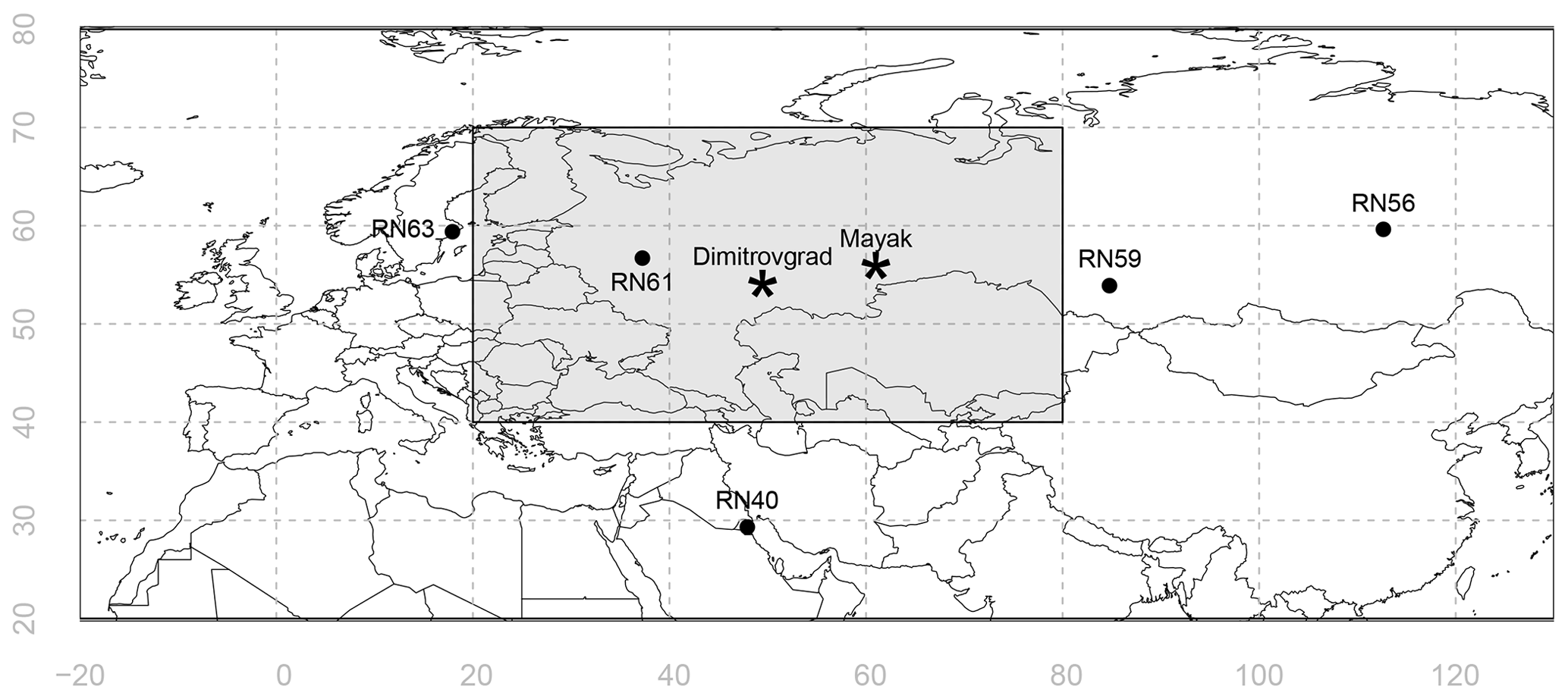
Figure 1Locations of the five stations from which 106Ru detections have been used. The shaded box shows the search domain of the Bayesian inference. For reference, the locations of two nuclear facilities are also shown: the Research Institute of Atomic Reactors in Dimitrovgrad, labelled “Dimitrovgrad” (54.19∘ N, 49.48∘ E) and the Mayak Production Association in Ozyorsk, labelled “Mayak” (55.70∘ N, 60.80∘ E).
2.1 Activity concentration observations
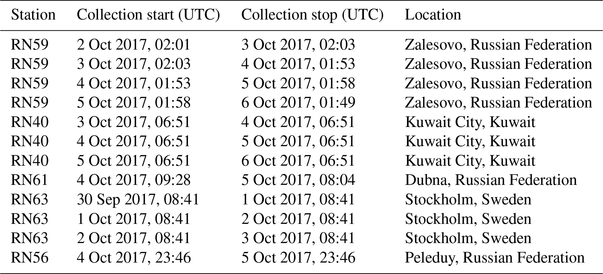
A total of 12 106Ru detections have been used from five different stations of the International Monitoring System, which is being commissioned to verify compliance with the Comprehensive Nuclear-Test-Ban Treaty once it enters into force. The observations, with their associated sampling times, are listed in Table 1. The location of these stations are shown in Fig. 1. The stations sample approximately 20 000 m3 of air during a period of 24 h, during which radioactive particulates – if present – are captured on a filter. The filter is then analyzed using gamma spectroscopy to detect the presence of any radionuclides. A few stations also measured 103Ru, but these detections will not be used for the inference. Although the observations were selected to realistically represent this case, we do not attempt to use all (or some optimal selection) of the available detections and non-detections in the inference as it is not our goal to determine the true source location as such. Furthermore, many additional observations contain redundant information. Also, since this work is focussed on Comprehensive Nuclear-Test-Ban Treaty verification applications, we only use a few observations taken at stations from the International Monitoring System. Finally, local observations in Russia could heavily influence the inferred source location, but we do not use these as our numerical weather ensemble is not well suited to capturing uncertainties at these smaller spatial and shorter temporal scales.
Table 1List of 12 observations with their corresponding sampling times and location.
2.2 Numerical weather prediction and atmospheric transport modelling
We have used the source–receptor sensitivities associated with the 12 observations from De Meutter et al. (2020). These were obtained by running the Lagrangian particle model Flexpart (Stohl et al., 2005) in backward mode (Seibert and Frank, 2004). All simulations ended on 20 September 2017. The source–receptor sensitivities represent the residence time of modelled particles in a geotemporal grid box. The time-averaged source–receptor sensitivities were output every 3 h, and thus the maximum possible residence time in a geotemporal grid box is 10 800 s. The source–receptor sensitivities have horizontal grid spacings of 0.5∘. An activity concentration (in Bq/m3) can be related to a release (in Bq) by multiplying the latter with the source–receptor sensitivity (in s) and dividing by the grid box volume and the source–receptor sensitivities averaging period (which was 10 800 s). An ensemble of numerical weather predictions was used to create an ensemble of atmospheric transport and dispersion simulations. The transport and dispersion processes themselves were not perturbed. The Ensemble of Data Assimilations from the European Centre for Medium-Range Weather Forecasts (ECMWF) was used to run Flexpart. It consists of 26 independent lower-resolution 4D-Var assimilations: one using unperturbed observations and physics and 25 using perturbed observations, sea surface temperatures, and model physics (Bonavita et al., 2016). The Ensemble of Data Assimilations (EDA) system uses a Gaussian grid with 640 latitude lines between pole and Equator, but the data were converted to a long–lat grid having grid spacings of 0.5∘. By adding and subtracting perturbations from the ensemble mean, the number of perturbed members was doubled, and thus 50 perturbed and 1 unperturbed member were obtained. The perturbations are created in such a way that each ensemble member represents a possible scenario for the true (unknown) atmospheric state, and the spread between the different members is simply the model uncertainty as estimated by the ensemble. Following this, for each weather ensemble member, Flexpart was run so that an atmospheric transport ensemble of 51 source–receptor sensitivities was obtained.
De Meutter and Hoffman (2020) have developed and applied a Bayesian inference system to find the source parameters of an anomalous 75Se release based on airborne 75Se activity concentrations. The main components of the inference system are summarized here, but details are given in De Meutter and Hoffman (2020) and references therein.
3.1 Source parameters
The unknown source is described by the following five source parameters:
-
the longitude of the source (xs),
-
the latitude of the source (ys),
-
the accumulated release (Q),
-
the release start time (tstart),
-
the release end time (tstop).
In practice, the release period is parameterized by fractions rstart and rstop to ensure that tstart occurs before tstop. The corresponding release period is calculated as follows:
with t1 and tm the first and last time for which source–receptor sensitivities are available for the source reconstruction. The release rate is assumed to be constant during the release period. The vertical position of the source is assumed to stretch between the surface and the top of the lowest model layer (at 100 m). Thus, the unknown source is parameterized as follows:
with δ the Dirac delta function and ℋ the Heaviside step function.
3.2 Prior distribution
Uninformative bounded uniform priors are used for the source parameters. The prior is designed to allow for all plausible scenarios given the sparse measurement network and under the assumption the detected radionuclides are from the same release. For the current study, the source longitude is assumed to be between 20 and 80∘ and the source latitude is assumed to be between 40 and 70∘ (see Fig. 1 for a map showing the search domain). The accumulated release is assumed to be between 1010 Bq and 1016 Bq. Since this spans many orders of magnitude, we take log 10(Q) as source parameter in our implementation and simply use a uniform distribution between 10 and 16 as uninformative prior. Recall that the first observation that we consider for the inference was taken on 1 October 2017. Therefore, the release is assumed to have occurred between 25 September 2017, 00:00 UTC, and 28 September 2017, 00:00 UTC. Generally, the upper limit on the release time will exclude solutions further downwind, while the lower limit on the release time will exclude solutions further upwind. Uniform bounded priors between 0 and 1 are used for rstart and rstop.
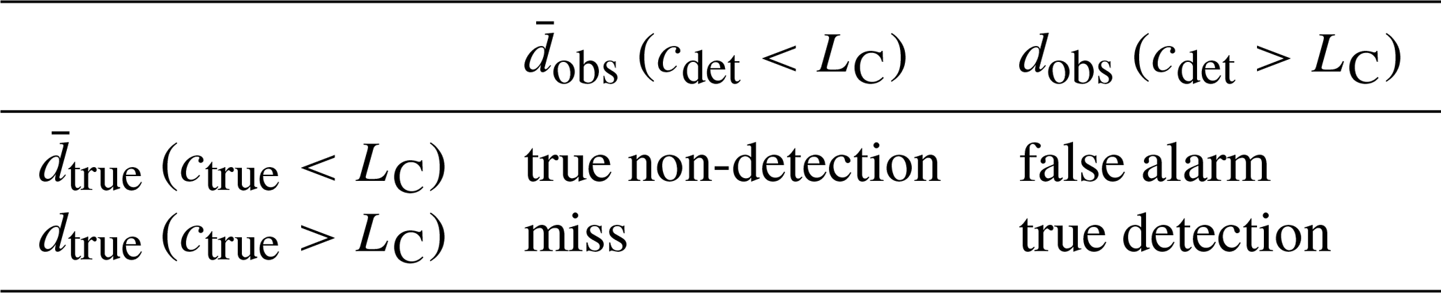
Table 2Definition of a true non-detection, a miss, a false alarm, and a true detection based on the Currie critical level LC, the detected activity concentration cdet, and the “true” activity concentration ctrue, which will never be known.
3.3 Likelihood
De Meutter and Hoffman (2020) proposed likelihood equations that can take into account detections, instrumental non-detections, misses and false alarms using Currie detection limits (Currie, 1968). Since non-detections will not be used in this study, only the likelihood of detections will be used here. The possibility of a false alarm, where the detector wrongly identifies a detection, is also considered. For simplicity, the observations cdet are assumed to be independent, thereby neglecting possible geotemporal correlations. As a result, the total likelihood is simply the product of the likelihood associated with individual observations:
First, let us define ctrue, which is the true activity concentration that will never be known. Next, we define cdet, which is the activity concentration as seen by the detector and which can differ from ctrue (the observed net signal can even be negative due to the statistical nature of spectroscopic analysis). Currie (1968) defined a critical level LC above which a net signal (which is the detected signal from which the effects of background radiation are subtracted) should be in order to declare the net signal to be a detection. We use this Currie critical threshold LC to decide, given a net signal, whether a real detection took place (dobs if cdet>LC) or not ( if cdet<LC). One can then define a true non-detection, a miss, a true detection and a false alarm as in Table 2. In this application, the risk of a missed detection and a false alarm is set equal to 5 %. ctrue will never be known, but we assume that the modelled activity concentration cmod corresponding to a source hypothesis Ξ and its associated uncertainty results in a distribution of true activity concentrations given by the following formula:
with the index i denoting “corresponding to the ith observation” (with i=1…12); Γ the gamma function; and s, , and parameters of an inverse gamma distribution. The above equation was used by Yee (2012) as a likelihood function for detections, and was obtained by starting from a Gaussian function, replacing the standard deviation σ with an inverse gamma distribution and integrating over all possible values of σ. However, in order to take into account the possibility of a false alarm, instead we propose the following likelihood for the ith detection cdet,i given its corresponding modelled activity concentration cmod,i associated with a source hypothesis Ξ:
In the equation above, p(dtrue|cmod) is the probability of a true detection, given by
and is the probability of a true non-detection, given by
In these equations, p(ctrue|cmod) is simply equal to Eq. (5) but is normalized (below, is a dummy variable for integration).
gives the likelihood of detecting cdet,i given cmod,i and assuming that the detection was not a false alarm. We assume it is given by Eq. (5) as follows.
is the likelihood of detecting cdet,i assuming that the detection is a false alarm:
with kα=1.645 for a false alarm risk of 5 %. The likelihood and its different components are plotted for two hypothetical detections in Fig. 2. For the hypothetical detection cdet close to its LC (Fig. 2, left), the likelihood is significantly increased for small cmod because the possibility of a false alarm is considered. For a hypothetical detection cdet significantly larger than its LC (Fig. 2, right), the consideration of a false alarm does not significantly add to the total likelihood. Indeed, for and , Eq. (6) simplifies to
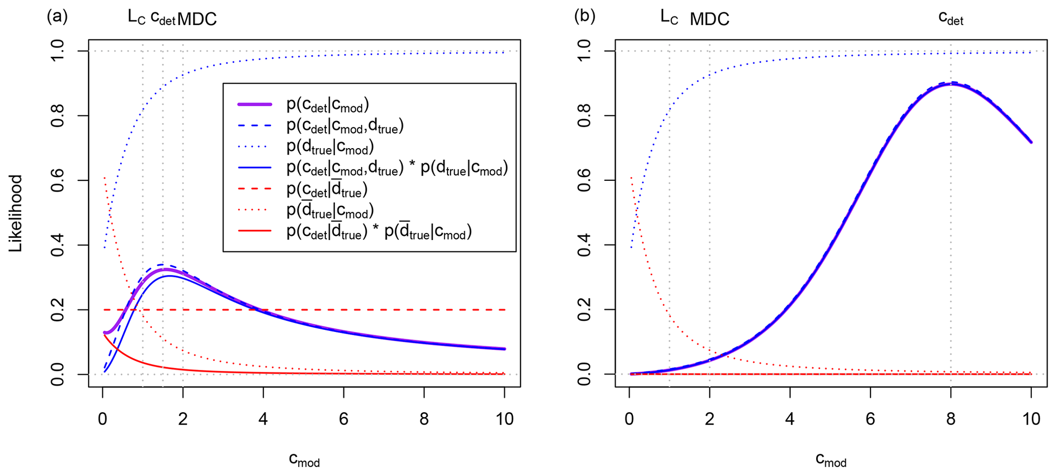
Figure 2Likelihood function for two detections: cdet=1.5 (a) and cdet=8.0 (b). The dotted vertical grey lines represent LC=1.0, MDC=2.0 and the detected activity concentration cdet. The units are arbitrary in this example.
3.4 Sampling from the posterior
The posterior distribution was sampled using the general-purpose Markov chain Monte Carlo algorithm MT-DREAM(ZS) (Laloy and Vrugt, 2012). A chain of source hypotheses is obtained by repeatedly creating a proposal source hypothesis based on the current source hypothesis and then accepting the proposal or – if it is rejected – retaining the current source hypothesis. A key feature of a Markov chain Monte Carlo algorithm is its ability to construct proposals in such a way that the posterior distribution is efficiently explored and sampled. MT-DREAM(ZS) creates a new proposal by adding a perturbation to the current source hypothesis. Such perturbations are created by taking the difference of two randomly drawn states out of an archive of past states so that the size and direction of the perturbation are adaptive and optimal for the problem – without the necessity of prior tuning. Every 10th iteration, the current source hypothesis is added to the archive. Three chains are run simultaneously (sharing the same archive of past states) to diagnose convergence more easily. To enhance efficiency and to obtain more accurate results, randomized subspace sampling is used (Vrugt et al., 2009). This simply means that not necessarily all source parameters are updated at a time, but instead a randomized subset of the source parameters are updated. Furthermore, MT-DREAM(ZS) makes use of multiple-try Metropolis sampling (Liu et al., 2000) to enhance the mixing of the chains. This means in practice that to advance to Markov chain several proposals are drawn instead of one proposal as in traditional Metropolis sampling. Furthermore, the Metropolis acceptance is calculated in a modified way (Liu et al., 2000; Laloy and Vrugt, 2012).
3.5 Observation and model errors
The detected activity concentration cdet is assumed to be Gaussian distributed around the true activity concentration ctrue, with a standard deviation σobs equal to the reported observation error. The model error originates from errors in the source–receptor sensitivities calculated by the atmospheric transport model. The main sources of error are simplifications in the turbulence parameterization of the atmospheric transport model and errors in the numerical weather prediction data used to run the atmospheric transport model. As it is very hard if not impossible to specify the model error, we assume Gaussian errors but replace a fixed σmod with an inverse gamma distribution, as mentioned earlier in this section and following Yee (2012):
with the subscript i denoting that these values can be observation-specific. The parameters s, and of the inverse gamma distribution are, respectively, an estimate of σmod, a scale parameter and a shape parameter. Yee (2012) proposed using and , in which case and the variance of σmod,i becomes infinite (Eq. 16 will then be a very heavy-tailed distribution). We now have to come up with a value for si. Since the source–receptor sensitivities or SRSs (calculated by the Flexpart model) typically span many orders of magnitude, it makes more sense to define a relative error rather than an absolute error. Furthermore, because the source–receptor sensitivities are linearly proportional to the activity concentration, we propose the following for si:
σsrs is the unknown SRS error in the equation above. The value of 16 is an empirical number that was found to give a good balance between information obtained from detections versus information from non-detections (De Meutter and Hoffman, 2020). Note that the above proposal results in a larger relative model error if . This is desirable since small detections are caused by a part of the plume of radionuclides that was subject to more atmospheric dilution and thus should have a larger relative uncertainty than large detections (although the latter have higher absolute uncertainty). In Eq. (13) (which is simply Eq. 5 but with ctrue replaced by cdet,i), si is replaced by the following in order to take into account both observation and model error:
From now on, we will express any parameters si and σ (the combined observation and model error) as relative errors and thus as fractions of (see Eq. 17).
In this section, only the unperturbed member is used. The model uncertainty thus needs to be specified manually, and the impact of different choices on the posterior is discussed here. We focus on the inferred source location and not the release period or release amount. This is because the release location is of primary interest in the context of treaty verification. Once a location is found (for instance, based on the location of known nuclear facilities within the posterior source region or based on a seismic signal associated with a nuclear explosion), a new inference could be performed fixing the release location as was done in De Meutter and Hoffman (2020).
4.1 Posterior effects
In this section, the effect of model error on the posterior is illustrated by varying the parameter si of the inverse gamma function (Eq. 16), which roughly fixes the scale of the model uncertainty. The Bayesian inference was independently repeated multiple times, once for each of the chosen parameter values. The resulting source location probability maps are shown in Fig. 3a, c, e for three values of si: 0.3, 0.5, and 3. Here, the same value si is used for all observations. The source location probability maps illustrate that the model error has a profound impact on the resulting posterior. The source location probability ranges from a narrow spot to a fairly elongated area. Perhaps surprisingly, an increase in the uncertainty parameter s does not simply enlarge the region of possible sources: instead, the enlargement is mostly in one direction (northeast); furthermore, the area with the highest probability shifts to the northeast. Therefore, one cannot simply predict beforehand how the posterior will change when the model error is changed. The resulting source location is in line with what previous studies found (Sørensen, 2018; Saunier et al., 2019; Bossew et al., 2019; De Meutter et al., 2020).
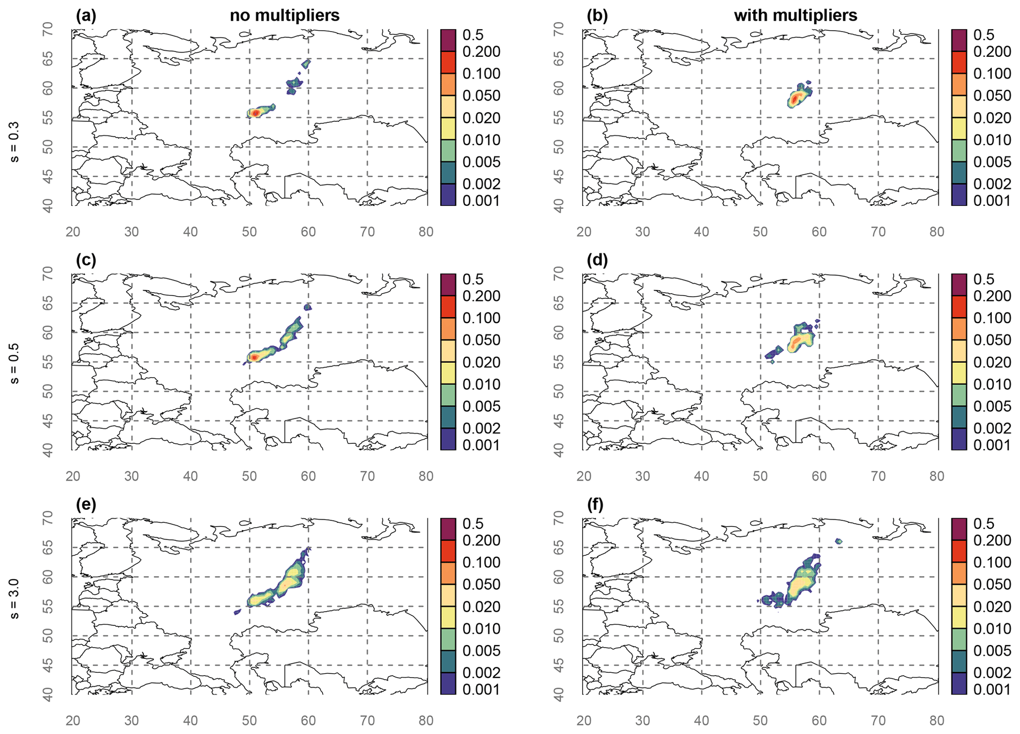
Figure 3Source location probability maps obtained from the Bayesian source reconstruction. The model uncertainty parameters of the inverse gamma distribution were fixed a priori, and different values for s were used in the panels: s=0.3 in (a), (b), s=0.5 in (c), (d) and s=3.0 in (e) and (f). No multipliers were used in (a), (c) and (e), while multipliers were used in panels (b), (d) and (f) (see Sect. 4.3 for details). The longitude and latitude are shown by grey numbers and dashed lines.
4.2 Introduction to multipliers
In this and the next subsection, an alternative model error structure will be discussed involving multipliers or scale factors. Besides being an alternative model error, multipliers could also be used to take into account errors that were not fully captured by the model (such as errors due to local atmospheric features not resolved by the model, measurement errors due to sample inhomogeneity)
Yee et al. (2014) used a small number of activity concentration measurements to retrieve the known source parameters of a major medical isotope production facility. The resulting source longitude, latitude and the release term were compared with the true source parameters in order to evaluate the performance of the source reconstruction. The method they used is similar to the method employed here: a Lagrangian stochastic particle model was used in backward mode to generate the source–receptor sensitivities, and the source parameters were obtained using Bayesian inference and the MT-DREAM(ZS) algorithm. Yee et al. (2014) showed that the main challenge in source reconstruction lies in the correct specification of the model uncertainty (both scale and structure) by using two different measurement models:
In Eq. (19), ϵi is the combined model and measurement error, which is assumed to be drawn from a Gaussian distribution with unknown standard deviation. Again, the unknown standard deviation is replaced by a distribution rather than a single fixed value. In Eq. (20), only represents the measurement error. The model error is now taken into account by so-called scale factors or multipliers mi. These multipliers are parameters of the Bayesian inference, and they are allowed to vary between 0.1 and 10. The range is chosen so that the multipliers can compensate for model underpredictions or overpredictions of up to a factor 10.
Yee et al. (2014) found that using Eq. (19) resulted in a source reconstruction that did not include the correct source parameters. The multipliers (Eq. 20) on the other hand resulted in a huge shift in the posterior source location, which significantly improved the source reconstruction.
4.3 Multipliers as unknown model error
Here, multipliers (mi) are introduced to account for unknown model uncertainties that are not yet taken into account by the likelihood formulation. For instance, local atmospheric features that are not resolved by the model might result in incorrect source–receptor sensitivities. Such errors are very hard to quantify because the computational power to resolve such features is prohibitively high (at least for continental-scale problems).
The multipliers are additional parameters that need to be estimated during the Bayesian inference. For the sampling of the parameter, we work with log 10(mi) and assign a uniform prior between . While the multipliers increase the run time of the Bayesian inference, the increase is small – especially if one considers the huge increase in the number of unknown parameters (one additional parameter per observation).
We apply the multipliers using three different values for the model uncertainty parameter si (0.3, 0.5 and 3) and show the results in Fig. 3b, d and f. Somewhat similar to the results in Yee et al. (2014), the multipliers cause a shift in the source location probability (though not as dramatic). Furthermore, the multipliers do not cause a widening in the posterior source location. It is interesting to contrast the effect of introducing the multipliers versus increasing the value of the parameter si: while the latter result in a shift and a widening of the posterior distribution, the former only result in a shift. While the results with and without multipliers are significantly different for small values of si (Fig. 3a and b), there is substantial agreement in the results when using si=3.0 (Fig. 3e and f). This suggests that the effect of introducing multipliers and the effect of increasing the model uncertainty converges when specifying large model uncertainty.
The results in this section lead to the following question: which of the source location maps shown in Fig. 3 is correct? More fundamentally, what is the true structure and scale of the model uncertainty? This will be assessed in the next section using the ensemble of source–receptor sensitivities described in Sect. 2.2.
5.1 The source–receptor sensitivity ensemble distribution
In this subsection, it is assessed whether the atmospheric transport model error structure can be obtained from the ensemble of source–receptor sensitivities (SRSs). Note that the ensemble is set up to deal with errors arising from the meteorological input data only. While this type of error likely adds the largest contribution to the total model error, other sources of model error are not included.
As our ensemble contains 51 members (one unperturbed member and 50 perturbed members), there are 51 SRS values available for each spatio-temporal grid box and each observation. In order to obtain the error structure, the data of all spatial grid boxes are aggregated into an uncertainty distribution. This does not necessarily destroy the spatial error correlations in the numerical weather prediction data, since the SRS are the result of an integrated trajectory through the atmosphere associated to a specific observation. The following procedure is applied in order to find the error structure.
-
For each SRS file (associated with a certain observation) and for each spatio-temporal grid box, the ensemble median SRS is calculated; each of the 51 SRS values is scaled by its ensemble median.
-
A Lagrangian particle model can only track a finite number of particles due to computational constraints, and this causes stochastic uncertainty when there are very few particles passing through a geotemporal grid box. However, the SRS variations between ensemble members should represent meteorological uncertainty and should not be impacted by stochastic uncertainty. Therefore, a threshold2 of exp (−20) [s] is applied to the median: if the median is smaller than the threshold, all of its 51 SRSs are omitted from the analysis.
-
The natural logarithm is applied to all SRSs since these span many orders of magnitude. If any ensemble member has an SRS equal to 0 for a specific grid box, all its 51 SRSs are omitted from the analysis.
-
The remaining data points are used to make an uncertainty distribution (as in Fig. 4).
As an example, the probability density function of ensemble SRS members around its ensemble median is shown in Fig. 4 for an arbitrary observation and an arbitrary time. It can be seen that most SRS values fall within a factor exp (3)≈20 of the ensemble median. Of particular interest is how this density can be approximated by a statistical distribution. In Fig. 4, two distributions are fitted to the density: a Gaussian distribution and a fit using Eq. (5). Interestingly, while the probability density function can roughly be represented by a Gaussian distribution (effectively being a lognormal distribution with respect to the SRS, since the natural logarithm was applied), its tails are heavier than a Gaussian distribution. On the other hand, a much better fit is obtained using Eq. (5). This distribution describes how the (unknown) true activity concentration is distributed on average around the modelled activity concentration. Similarly, the ensemble gives a distribution of the true SRS around the model-predicted SRS. Note that the activity concentrations are simply linear combinations of SRS. This result shows that our choice for the model error structure is supported by the ensemble. This initial result will be elaborated in the next subsection.
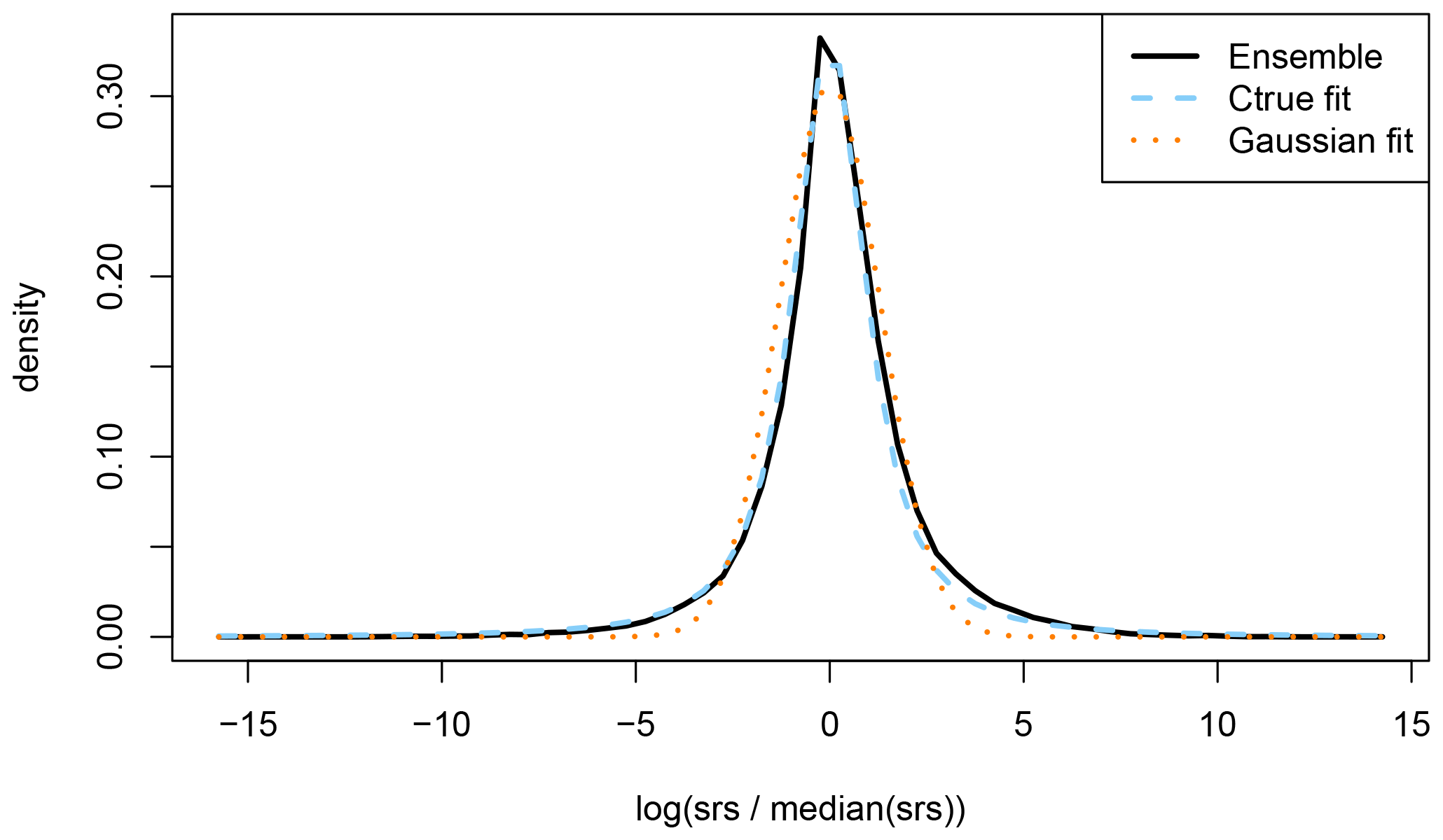
Figure 4Probability density function showing how the atmospheric transport model ensemble members are distributed around the ensemble median (solid black line). Also shown are two fits, one using Eq. (5) (dashed blue line) and one using a Gaussian distribution (dotted orange line). Note that the SRSs are scaled by its ensemble median and that the natural logarithm is applied.
5.2 Fitting model uncertainty
In this subsection, the SRS ensemble is used to determine the parameters si, and in Eq. (5), which describes how the true activity concentration ctrue is believed to be distributed given the modelled activity concentration cmod,i. The fitting can be performed in several ways, and four different cases are considered. A goodness-of-fit is calculated for each case. As a reference, the fitting procedure is repeated using a Gaussian distribution instead of Eq. (5). The mean of the Gaussian is fixed to be 0 (corresponding to the median of the SRS ensemble) so that only the standard deviation is allowed to vary. Since our Gaussian fitting thus has only one degree of freedom (and given the suggestion of long tails in Fig. 4), it should not be surprising that the Gaussian fit will be outperformed by the fit using Eq. (5).
The following cases are considered to obtain the uncertainty parameters.
-
Case 1: the parameters are fixed by a priori chosen values; for the fit using Eq. (5), we choose si=0.5, , and for all observations and all 3 h release time intervals; for the Gaussian distribution, we choose σ=0.5.
-
Case 2: the parameters are fitted once for all release time intervals and all observations (data are aggregated for all release times and all observations).
-
Case 3: the parameters are fitted for each observation (data are aggregated for all release time intervals).
-
Case 4: the parameters are fitted for each observation and each release time interval.
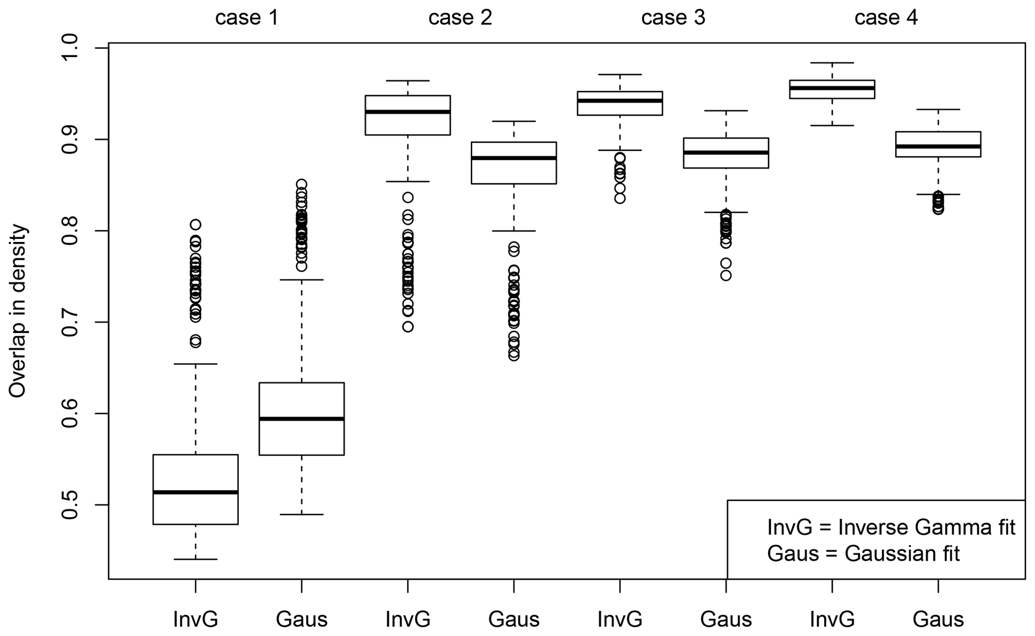
The following goodness-of-fit is chosen to quantify how well the fitted probability density function pfit resembles the ensemble probability density function pens; it involves the integration of the absolute difference of both densities and is simply the fraction of overlap in density:
If the overlap in density equals 1, pfit equals pens. On the other hand, if it equals 0, there is no overlap between pfit and pens.
The uncertainty parameters are obtained using the procedures outlined in cases 1 to 4. Following this, for each case the overlap in density is calculated by comparing pfit with pens for each observation and each release time interval separately, resulting in 288 data points since there are 24 different release time intervals and 12 observations. The set of overlap in densities is used to construct box plots in Fig. 5. The overlap in density is poor when using the a priori values for the uncertainty parameters (labels “InvG” and “Gaus”, case 1 in Fig. 5). While the outcome would have been entirely different if better a priori values would have been chosen, its significance should not be underestimated: (i) although seemingly realistic a priori uncertainty parameters have been chosen, the agreement with the ensemble density is poor. (ii) For this case and this particular choice of uncertainty parameters, a Gaussian distribution resulted in a better agreement. (iii) In the absence of an ensemble, using uncertainty parameters that are chosen a priori might be the only available option. When fitting the uncertainty parameters once for all observations and all release time intervals, the overlap in density is significantly improved (labels “InvG” and “Gaus”, case 2 in Fig. 5). The fit using Eq. (5) performs significantly better than the Gaussian fit. Additional smaller improvements are obtained when fitting for each observation separately (labels InvG and Gaus, case 3 in Fig. 5) and when fitting for each observation and release time interval separately (labels InvG and Gaus, case 4 in Fig. 5).
5.3 Error dependency on the release time interval and the observation
In this subsection, it is assessed how the fitted uncertainty parameters vary among different observations and different release time intervals. The motivation for this is as follows: first (somewhat trivially), we can expect the model uncertainty to increase as a function of simulation time. Second, uncertainties are expected to be observation-dependent, since observations are made on different times and at different distances from the source; uncertainties on the trajectories between the receptor and the source will also be affected by the atmospheric conditions along the trajectory, which are expected to be observation-specific. The interplay of the three uncertainty parameters s, and of the inverse gamma function make it less feasible to directly estimate any effect. Therefore, only the fitted standard deviations of the Gaussian distribution are considered here.
The fitted standard deviation for each observation (averaged over all release time intervals) is shown in Fig. 6 (left). The standard deviation varies significantly between the different observations – up to a factor of 2 between the 3rd and the 11th observation. This can alter the posterior since the uncertainty scales how deviations between the simulated and observed activity concentration are penalized. While it appears difficult to assign meaningful observation-specific a priori uncertainty parameters, the ensemble can readily provide such information.
The fitted standard deviation for each release time interval (averaged over all observations) is shown in Fig. 6 (right). It can be seen that the model uncertainty grows when going backwards in time. The growth is about 30 % during a 3 d period (note that such growth does not have to be constant over time, and an in-depth assessment is out of the scope of this paper). Also interesting to note is that there is an oscillatory behaviour with a period of eight time steps, corresponding to the diurnal cycle (since SRS fields were produced every 3 h). The oscillations are likely associated with boundary layer processes, which often follow the diurnal cycle.
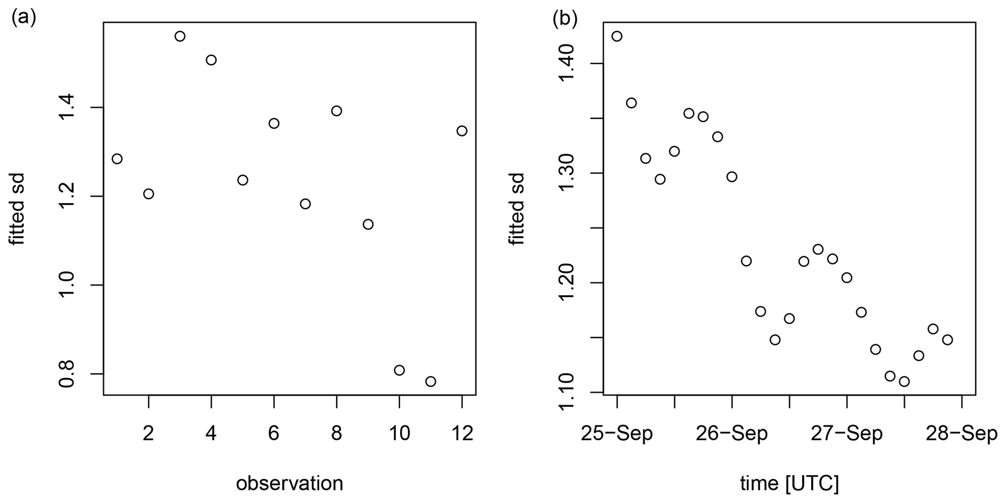
Figure 6The standard deviation obtained after fitting a Gaussian distribution to the SRS ensemble. (a) Standard deviation fitted for each of the 12 observations (all release time intervals are aggregated); the indices of the observations on the x axis are arbitrary. (b) Standard deviation fitted for each of the 24 release time intervals (all observations are aggregated); each release time interval is 3 h long.
5.4 Resulting source location probability map
In this subsection, the Bayesian source reconstruction is applied using fitted observation-specific parameters si, and (this corresponds to case 3, invG in Fig. 5). Furthermore, the inference is run using the SRS ensemble median for each geotemporal grid box – prior to this the unperturbed ensemble member was used. The resulting probability map is shown in Fig. 7a. While the source location probability map is distinct from (most of) the individual panels shown in Fig. 3, it is not too different from what Fig. 3 as a whole suggests. It best resembles Fig. 3f, which corresponds to the combination of multipliers with large model uncertainty. Note that simply changing the a priori uncertainty parameters might never yield a near-perfect correspondence with Fig. 7a, since the fitting resulted in different uncertainty parameters for each observation, which seems impossible to obtain without an ensemble.
For comparison, the average probability of the six panels in Fig. 3 is shown in Fig. 7b. The latter is perhaps the best approach one can take in the absence of an ensemble. While both maps roughly agree at first glance, there are still important differences. Foremost, the most southwest mode out of two modes in Fig. 7b is absent in Fig. 7a. The other mode in Fig. 7b is slightly shifted to the west in Fig. 7a and extends further northeast.
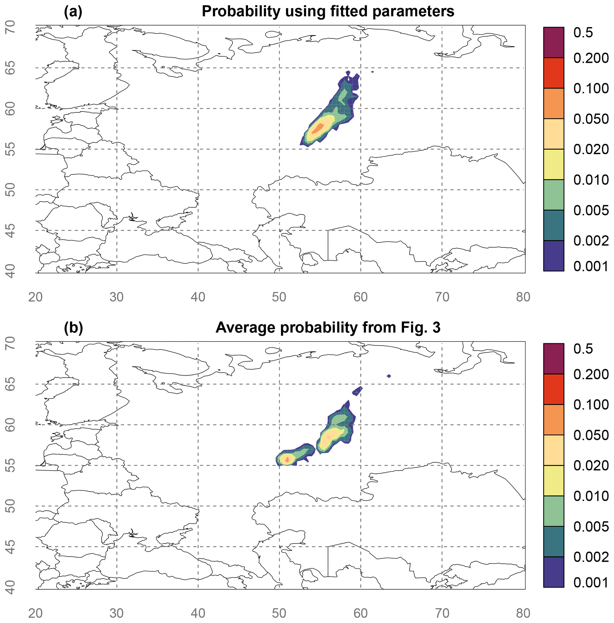
Figure 7Source location probability map obtained from the Bayesian source reconstruction. (a) The parameters of the inverse gamma distribution were obtained using the ensemble SRS for each observation separately. (b) The average source location probability is taken from all six panels shown in Fig. 3. The longitude and latitude are shown by grey numbers and dashed lines.
In this section, it is assessed whether additional information can be acquired by considering each ensemble member as an independent scenario, thus performing the Bayesian source reconstruction for each ensemble member separately. No fitting of uncertainty parameters is applied here, and thus these need to be set a priori. The experiment is performed twice, once using si=0.5 and once using si=3.0. The other two uncertainty parameters remain fixed ( and ).
6.1 Source location probability maps
The Bayesian inference is repeated using the SRS of each ensemble member, so that 51 different posteriors are obtained. These posteriors then need to be aggregated in some way. As before, we focus on the source location probability. While several aggregation methods are possible, here the grid-box-wise mean and maximum probability is taken (normalization is required to ensure that the probabilities sum up to 1). Equal weights were assigned to each ensemble member, since our ensemble is constructed to yield equally likely scenarios or ensemble members. Note that in the case of multi-model ensembles, the latter might not be true, and thus a weighting should be applied based on the skill of each model.
Figure 8a and b show the results using the unperturbed member only and using si=0.5 and si=3.0; hence, these are identical to Fig. 3c and e. As discussed earlier in Sect. 4, the source location probability map differs significantly when changing the parameter s. Figure 8c and d show the results for the grid-box-wise ensemble mean using si=0.5 and si=3.0. The results are slightly broader and much smoother, not showing significant bimodal behaviour. Two features are noteworthy: first, the results roughly approximate those in Fig. 7, though important differences are present, as there were between Fig. 7a and b. Second, the results are generally insensitive to the choice of the uncertainty parameter s, since Fig. 8c and d are very similar. The same is true for Fig. 8e and f, which show the grid-box-wise ensemble maximum. As one can expect, the resulting source location probability is slightly broader than the one obtained by taking the grid box mean probability; however, the differences are minor.
It seems that overall a similar picture is obtained when running the Bayesian inference for each ensemble member separately compared to the procedure explained in Sect. 5. This suggests that if we use the ensemble only (i) to fit the uncertainty parameters and (ii) to calculate the ensemble median SRS for running the inference as was done in order to obtain Fig. 7, no crucial information from the ensemble is lost with respect to the source location. As a consequence, it is equivalent to running the inference with all members of the ensemble separately to determine the uncertainty.
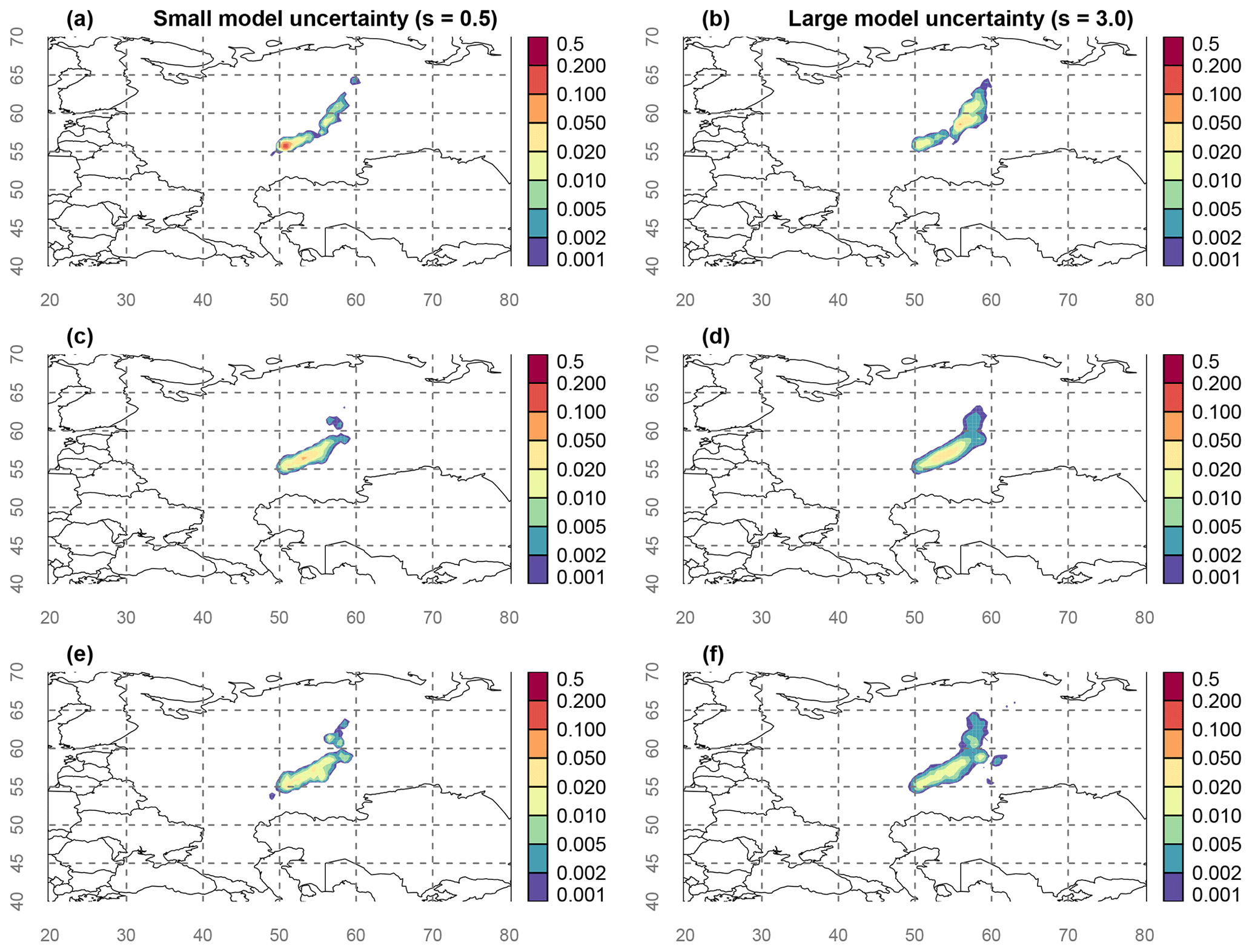
Figure 8Source location probability maps for (a), (b) the unperturbed member; (c), (d) the grid-box-wise ensemble mean; and (e), (f) the grid-box-wise ensemble maximum. Panels (a), (c), and(e) were obtained using s=0.5; panels (b), (d), and (f) were obtained using s=3.0. The longitude and latitude are shown by grey numbers and dashed lines.
6.2 Ensemble convergence
Finally, we perform a brief assessment on whether or not each ensemble member is adding new information to the ensemble mean source location probability. For each perturbed member , the overlap in source location probability is calculated between that member and the mean of all previous members (with member 0 the unperturbed member). We thus start with the first perturbed member (which is compared with simply the unperturbed member) and end with the last perturbed member (which is compared with the mean of all other ensemble members). The results are shown in Fig. 9 for an uncertainty parameter s=0.5 and an uncertainty parameter s=3.0. Note that the overlap in density is calculated using Eq. (21) and has the same meaning as before, with 0 denoting no overlap (thus being fully informative) and 1 denoting full overlap (providing no new information).
Figure 9 shows that most ensemble members have an overlap in density less than 0.6. There is significant variance in how much new information is added by each ensemble member. A linear fit suggests that the added information from additional ensemble members is slowly decreasing, as expected. Note that the effect is more pronounced for the case with higher model uncertainty (Fig. 9, right). The reason for this is that the source location probability is more spread out due to the higher model uncertainty, making an overlap more likely. We conclude that all ensemble members are adding new information. This is desirable, as it shows that the ensemble is well-constructed (if members are generally not adding new information, they could be a waste of computational resources).

Figure 9Overlap in source location probability as a proxy for how much new information each ensemble member is adding to the ensemble mean (see text). (a) Results obtained using an uncertainty parameter s=0.5. (b) Results obtained using an uncertainty parameter s=3.0. A linear fit is also plotted (solid black line).
Model error has a huge impact on the posterior obtained through Bayesian source reconstruction, a conclusion in agreement with other studies (e.g., Yee et al., 2014). Specifically for the source location, an increase in the scale of the model error resulted in a non-uniform broadening and a shift in the source location probability.
Both the non-uniformity of the broadening and the shift in the source location probability imply that one cannot simply predict beforehand what the result will be when the Bayesian source reconstruction is repeated with different model error.
In the absence of a way to determine the model error, one could perform multiple Bayesian source reconstructions using different model error formulations as shown in Fig. 3. The results could be aggregated by taking the average (as in Fig. 7b) or by using more elaborate procedures (including a weighted mean).
Multipliers can be used to represent model error (as in Yee et al., 2014) or to represent the unknown part of model error as was done in Sect. 4.3. The multipliers result in a shift in the source location probability but not in a broadening.
We found that the ensemble members of source–receptor sensitivities are distributed around their ensemble median (Fig. 4) in a way that can be well-described by Eq. (5); the latter describes how the true activity concentration ctrue is assumed to be distributed around the modelled activity concentration cmod. Therefore, an ensemble of atmospheric transport and dispersion simulations can be employed to determine the parameters associated with the inverse gamma function in Eq. (16). Of course, the effectiveness of such approach largely depends on whether the ensemble is capable of representing model error.
The ensemble showed that model error varies among different observations (up to a factor of 2 in the standard deviation when fitting a Gaussian distribution). Therefore, it is expected that having available model error information that is observation-specific can improve the quality of the Bayesian source reconstruction. The model error is also shown to increase when going further backward in time (for this specific case, there was an increase of 30 % during a 3 d period in the standard deviation when fitting a Gaussian distribution).
The source location probability using the fitted model error obtained from the ensemble (Fig. 7a) is distinct from the source location probability obtained using fixed uncertainty parameters (individual panels in Fig. 3); however, it is not too different from what Fig. 3 as a whole suggests, which demonstrates the usefulness of performing multiple Bayesian source reconstructions using different model error formulations as a sensitivity analysis in the absence of an ensemble.
A scenario-based approach (where each ensemble member is used as input for the Bayesian source reconstruction, instead of using the ensemble to fit the uncertainty parameters) gives results that are more robust against the choice of the uncertainty parameters but are more costly compared to directly fitting the uncertainty parameters. This is because the ensemble introduces model uncertainty that may predominate against the uncertainty prescribed by arbitrarily choosing the uncertainty parameter. No new information is obtained for the source location probability (in other words, one does not lose information when using the ensemble only to fit the uncertainty parameters and to calculate the ensemble median for use in the Bayesian inference). The scenario-based approach might be best in case of a small multi-model ensemble, since the fitting of uncertainty parameters might be difficult due to the difference in skill of each ensemble member.
In a future study, we will apply the different approaches and methods presented in this paper to situations in which the source characteristics are known unambiguously. This will help to better evaluate the different approaches proposed in this paper.
The Flexpart model that was used to generate the SRS data is open source and is available for download (Flexpart, 2020, https://www.flexpart.eu/, last access: 1 September 2020). The SRS data from the Flexpart model are available on Zenodo (De Meutter and Delcloo, 2020, https://doi.org/10.5281/zenodo.4003640). The Bayesian inference tool is available under the GPL3 and can be downloaded from Zenodo (https://doi.org/10.5281/zenodo.4588282, De Meutter et al., 2021). More recent versions of the code will be published on GitLab.com (https://gitlab.com/trDMt2er/FREAR, last access: 24 February 2021).
The supplement related to this article is available online at: https://doi.org/10.5194/gmd-14-1237-2021-supplement.
All authors contributed to the conceptualization of the study. PDM conducted the simulations and performed the analysis. IH and KU supervised the research. All authors contributed to the manuscript. IH took care of the project administration.
The authors declare that they have no conflict of interest.
The authors would like to thank the reviewers for their constructive comments.
This research has been supported by the Defense Research and Development Canada's Canadian Safety and Security Program (project no. CSSP-2018-TI-2393).
This paper was edited by Slimane Bekki and reviewed by Patrick Armand and two anonymous referees.
Becker, A., Wotawa, G., De Geer, L.-E., Seibert, P., Draxler, R. R., Sloan, C., D'Amours, R., Hort, M., Glaab, H., Heinrich, P., Grillon Vyacheslav Shershakov, Y., Katayama, K., Zhang, Y., Stewart, P., Hirtl, M., Jean, M., and Chen, P.: Global backtracking of anthropogenic radionuclides by means of a receptor oriented ensemble dispersion modelling system in support of Nuclear-Test-Ban Treaty verification, Atmos. Environ., 41, 4520–4534, https://doi.org/10.1016/j.atmosenv.2006.12.048, 2007. a
Bocquet, M.: High-resolution reconstruction of a tracer dispersion event: application to ETEX, Q. J. Roy. Meteor. Soc., 133, 1013–1026, https://doi.org/10.1002/qj.64, 2007. a
Bonavita, M., Hólm, E., Isaksen, L., and Fisher, M.: The evolution of the ECMWF hybrid data assimilation system, Q. J. Roy. Meteor. Soc., 142, 287–303, https://doi.org/10.1002/qj.2652, 2016. a
Bossew, P., Gering, F., Petermann, E., Hamburger, T., Katzlberger, C., Hernandez-Ceballos, M., De Cort, M., Gorzkiewicz, K., Kierepko, R., and Mietelski, J.: An episode of Ru-106 in air over Europe, September–October 2017–Geographical distribution of inhalation dose over Europe, J. Environ. Radioactiv., 205, 79–92, https://doi.org/10.1016/j.jenvrad.2019.05.004, 2019. a, b
Currie, L. A.: Limits for qualitative detection and quantitative determination. Application to radiochemistry, Analyt. Chem., 40, 586–593, https://doi.org/10.1021/ac60259a007, 1968. a, b
De Meutter, P. and Delcloo, A.: SRS data, Zenodo, https://doi.org/10.5281/zenodo.4003640, 2020. a
De Meutter, P. and Hoffman, I.: Bayesian source reconstruction of an anomalous Selenium-75 release at a nuclear research institute, J. Environ. Radioactiv., 218, 1–13, https://doi.org/10.1016/j.jenvrad.2020.106225, 2020. a, b, c, d, e, f
De Meutter, P., Camps, J., Delcloo, A., and Termonia, P.: Source localisation and its uncertainty quantification after the third DPRK nuclear test, Sci. Rep.-UK, 8, 10155, https://doi.org/10.1038/s41598-018-28403-z, 2018. a
De Meutter, P., Camps, J., Delcloo, A., and Termonia, P.: Source Localization of Ruthenium-106 Detections in Autumn 2017 Using Inverse Modelling, in: Mensink C., Gong W., Hakami A. (eds) Air Pollution Modeling and its Application XXVI. ITM 2018. Springer Proceedings in Complexity., Springer, Cham, https://doi.org/10.1007/978-3-030-22055-6_15, 2020. a, b, c, d
De Meutter, P., Hoffman, I., and Hladun, N.: FREAR source code, Zenodo, https://doi.org/10.5281/zenodo.4588282, 2021. a
Engström, A. and Magnusson, L.: Estimating trajectory uncertainties due to flow dependent errors in the atmospheric analysis, Atmos. Chem. Phys., 9, 8857–8867, https://doi.org/10.5194/acp-9-8857-2009, 2009. a
Flexpart: Flexpart, available at: https://www.flexpart.eu/, last access: 1 September 2020. a
Harris, J. M., Draxler, R. R., and Oltmans, S. J.: Trajectory model sensitivity to differences in input data and vertical transport method, J. Geophys. Res.-Atmos., 110, 1–8, https://doi.org/10.1029/2004JD005750, 2005. a
Hegarty, J., Draxler, R. R., Stein, A. F., Brioude, J., Mountain, M., Eluszkiewicz, J., Nehrkorn, T., Ngan, F., and Andrews, A.: Evaluation of Lagrangian particle dispersion models with measurements from controlled tracer releases, J. Appl. Meteorol. Climatol., 52, 2623–2637, https://doi.org/10.1175/JAMC-D-13-0125.1, 2013. a
Laloy, E. and Vrugt, J. A.: High-dimensional posterior exploration of hydrologic models using multiple-try DREAM (ZS) and high-performance computing, Water Resour. Res., 48, 1–18, 2012. a, b
Leutbecher, M.: Ensemble size: How suboptimal is less than infinity?, Q. J. Roy. Meteor. Soc., 145, 107–128, https://doi.org/10.1002/qj.3387, 2019. a
Leutbecher, M. and Palmer, T. N.: Ensemble forecasting, J. Comput. Phys., 227, 3515–3539, https://doi.org/10.1016/j.jcp.2007.02.014, 2008. a
Liu, J. S., Liang, F., and Wong, W. H.: The multiple-try method and local optimization in Metropolis sampling, J. Am. Stat. Assoc., 95, 121–134, 2000. a, b
Masson, O., Steinhauser, G., Wershofen, H., Mietelski, J. W., Fischer, H. W., Pourcelot, L., Saunier, O., Bieringer, J., Steinkopff, T., Hýža, M., Møller, B., Bowyer, T. W., Dalaka, E., Dalheimer, A., de Vismes-Ott, A., Eleftheriadis, K., Forte, M., Gasco Leonarte, C., Gorzkiewicz, K., Homoki, Z., Isajenko, K., Karhunen, T., Katzlberger, C., Kierepko, R., Kövendiné Kónyi, J., Malá, H., Nikolic, J., Povinec, P. P., Rajacic, M., Ringer, W., Rulík, P., Rusconi, R., Sáfrány, G., Sykora, I., Todorović, D., Tschiersch, J., Ungar, K., and Zorko, B.: Potential source apportionment and meteorological conditions involved in airborne 131I detections in January/February 2017 in Europe, Environ. Sci. Technol., 52, 8488–8500, https://doi.org/10.1021/acs.est.8b01810, 2018. a
Masson, O., Steinhauser, G., Zok, D., Saunier, O., Angelov, H., Babić, D., BeĊková, V., Bieringer, J., Bruggeman, M., Burbidge, C. I., Conil, S., Dalheimer, A., De Geer, L.-E., de Vismes Ott, A., Eleftheriadis, K., Estier, S., Fischer, H., Garavaglia, M. G., Gasco, Leonarte, C., Gorzkiewicz, K., Hainz, D., Hoffman, I., Hýža, M., Isajenko, K., Karhunen, T., Kastlander, J., Katzlberger, C., Kierepko, R., Knetsch, G.-J., Kövendiné Kónyi, J., Lecomte, M., Mietelski, J. W., Min, P., Møller, B., Nielsen, S. P., Nikolic, J., Nikolovska, L., Penev, I., Petrinec, B., Povinec, P. P., Querfeld, R., Raimondi, O., Ransby, D., Ringer, W., Romanenko, O., Rusconi, R., Saey, P. R. J., Samsonov, V., Šilobritienė, B., Simion, E., Söderström, C., Šoštarić, M., Steinkopff, T., Steinmann, P., Sýkora, I., Tabachnyi, L., Todorovic, D., Tomankiewicz, E., Tschiersch, J., Tsibranski, R., Tzortzis, M., Ungar, K., Vidic, A., Weller, A., Wershofen, H., Zagyvai, P., Zalewska, T., Zapata García, D., and Zorko, B.: Airborne concentrations and chemical considerations of radioactive ruthenium from an undeclared major nuclear release in 2017, P. Natl. Acad. Sci. USA, 116, 16750–16759, https://doi.org/10.1073/pnas.1907571116, 2019. a, b
Ringbom, A., Axelsson, A., Aldener, M., Auer, M., Bowyer, T. W., Fritioff, T., Hoffman, I., Khrustalev, K., Nikkinen, M., Popov, V., Popov, Y., Ungar, K., and Wotawa, G.: Radioxenon detections in the CTBT international monitoring system likely related to the announced nuclear test in North Korea on February 12, 2013, J. Environ. Radioactiv., 128, 47–63, https://doi.org/10.1016/j.jenvrad.2013.10.027, 2014. a
Saunier, O., Didier, D., Mathieu, A., Masson, O., and Le Brazidec, J. D.: Atmospheric modeling and source reconstruction of radioactive ruthenium from an undeclared major release in 2017, P. Natl. Acad. Sci. USA, 116, 24991–25000, https://doi.org/10.1073/pnas.1907823116, 2019. a, b
Seibert, P. and Frank, A.: Source–receptor matrix calculation with a Lagrangian particle dispersion model in backward mode, Atmos. Chem. Phys., 4, 51–63, https://doi.org/10.5194/acp-4-51-2004, 2004. a, b
Sørensen, J. H.: Method for source localization proposed and applied to the October 2017 case of atmospheric dispersion of Ru-106, J. Environ. Radioactiv., 189, 221–226, https://doi.org/10.1016/j.jenvrad.2018.03.010, 2018. a, b
Steinhauser, G.: Anthropogenic radioactive particles in the environment, J. Radioanal. Nucl. Ch., 318, 1629–1639, https://doi.org/10.1007/s10967-018-6268-4, 2018. a
Stohl, A., Forster, C., Frank, A., Seibert, P., and Wotawa, G.: Technical note: The Lagrangian particle dispersion model FLEXPART version 6.2, Atmos. Chem. Phys., 5, 2461–2474, https://doi.org/10.5194/acp-5-2461-2005, 2005. a
Stohl, A., Seibert, P., Wotawa, G., Arnold, D., Burkhart, J. F., Eckhardt, S., Tapia, C., Vargas, A., and Yasunari, T. J.: Xenon-133 and caesium-137 releases into the atmosphere from the Fukushima Dai-ichi nuclear power plant: determination of the source term, atmospheric dispersion, and deposition, Atmos. Chem. Phys., 12, 2313–2343, https://doi.org/10.5194/acp-12-2313-2012, 2012. a
Vrugt, J. A., Ter Braak, C., Diks, C., Robinson, B. A., Hyman, J. M., and Higdon, D.: Accelerating Markov chain Monte Carlo simulation by differential evolution with self-adaptive randomized subspace sampling, Int. J. Nonlin. Sci. Num., 10, 273–290, https://doi.org/10.1515/IJNSNS.2009.10.3.273, 2009. a
Yee, E.: Inverse dispersion for an unknown number of sources: model selection and uncertainty analysis, ISRN Applied Mathematics, 2012, 1–20, https://doi.org/10.5402/2012/465320, 2012. a, b, c, d
Yee, E., Hoffman, I., and Ungar, K.: Bayesian inference for source reconstruction: A real-world application, International scholarly research notices, 2014, 1–12, https://doi.org/10.1155/2014/507634, 2014. a, b, c, d, e, f, g
Anomalous radionuclide detections are detections of anthropogenic radionuclides originating from upwind nuclear facilities, where the detected concentration of (a) specific radionuclide(s) and/or the combination of several detected radionuclides are anomalous with respect to the station's detection history and/or with respect to what can be expected from these upwind nuclear facilities operating under normal conditions.
Since the SRS files are output every 3 h, the maximum value for the SRS is 10 800 s.
- Abstract
- Introduction
- Description of the case
- Bayesian source reconstruction
- Model error and Bayesian source reconstruction
- Fitting uncertainty parameters
- Ensembles as a set of scenarios
- Conclusions
- Code and data availability
- Author contributions
- Competing interests
- Acknowledgements
- Financial support
- Review statement
- References
- Supplement