Development of an atmospheric chemistry model coupled to the PALM model system 6.0: implementation and first applications

In this article we describe the implementation of an online-coupled gas-phase chemistry model in the turbulence-resolving PALM model system 6.0 (formerly an abbreviation for Parallelized Large-eddy Simulation Model and now an independent name). The new chemistry model is implemented in the PALM model as part of the PALM-4U (PALM for urban applications) components, which are designed for application of the PALM model in the urban environment (Maronga et al., 2020). The latest version of the Kinetic PreProcessor (KPP, 2.2.3) has been utilized for the numerical integration of gas-phase chemical reactions. A number of tropospheric gas-phase chemistry mechanisms of different complexity have been implemented ranging from the photostationary state (PHSTAT) to mechanisms with a strongly simplified volatile organic compound (VOC) chemistry (e.g. the SMOG mechanism from KPP) and the Carbon Bond Mechanism 4 (CBM4; Gery et al., 1989), which includes a more comprehensive, but still simplified VOC chemistry. Further mechanisms can also be easily added by the user. In this work, we provide a detailed description of the chemistry model, its structure and input requirements along with its various features and limitations. A case study is presented to demonstrate the application of the new chemistry model in the urban environment. The computation domain of the case study comprises part of Berlin, Germany. Emissions are considered using street-type-dependent emission factors from traffic sources. Three chemical mechanisms of varying complexity and one no-reaction (passive) case have been applied, and results are compared with observations from two permanent air quality stations in Berlin that fall within the computation domain. Even though the feedback of the model's aerosol concentrations on meteorology is not yet considered in the current version of the model, the results show the importance of online photochemistry and dispersion of air pollutants in the urban boundary layer for high spatial and temporal resolutions. The simulated NO_x and O₃ species show reasonable agreement with observations. The agreement is better during midday and poorest during the evening transition hours and at night. The CBM4 and SMOG mechanisms show better agreement with observations than the steady-state PHSTAT mechanism.

1 Introduction

More than half of the world's population lives in cities, and the number is expected to exceed two-thirds by the year 2050 (United Nations, 2014). The high population density in urban areas leads to intense resource utilization, increased energy consumption and high traffic volumes, which results in large amounts of air pollutant emissions. Various urban features such as the heterogeneity of building distribution, large amount of impervious material, scarcity of vegetation and street geometry can influence the atmospheric flow, its turbulence regime and the micro-climate within the urban boundary layer that accordingly modify the transport, chemical transformation and removal of air pollutants (Hidalgo et al., 2008). Air pollution has a multitude of complex effects on human health, material, ecology and environment. In order to develop policies and strategies to protect human health and environment, a better understanding of the interaction between air pollutants and the complex flow within the urban areas is necessary.

Air quality of a given region is strongly dependent on the meteorological conditions and pollutant emissions (Seaman, 2000; Jacob and Winner, 2009). In urban canopies, turbulence can modify pollutant concentrations both within and downstream of urban areas. Interactions between meteorology and chemistry are complex and mostly non-linear. Numerical models are useful tools to capture these interactions and help to understand the effect of meteorology on the chemical processes. Modelling of air quality on the regional scale has made major advances within the past decades (Baklanov et al., 2014). However, small-scale dispersion of pollutants from traffic and other sources within urban areas and their chemical and physical transformation are still poorly understood and difficult to predict due to uncertainty in emissions and complexity of modelling turbulence within and above the urban canopies. As well as this, the computational costs for including air pollution chemistry and physics in the models are remarkably high due to additional prognostic equations for chemical species and the corresponding chemical reactions.

Reynolds-averaged Navier–Stokes (RANS) based dispersion models are now widely used for assessing urban air quality by providing predictions of present and future air pollution levels as well as temporal and spatial variations (Vardoulakis et al., 2003; Sharma et al., 2017). In these models, atmospheric turbulence at the city level is primarily resolved by the Reynolds-averaged eddy-viscosity and the rate of turbulent kinetic energy dissipation (k-ε) where turbulence is fully parameterized and thus cannot provide information about turbulence structures and its consequent effects on the atmospheric chemistry (Meroney et al., 1995, 1996; Li et al., 2008). Some of these RANS models are able to resolve buildings and trees, e.g. MITRAS (the microscale obstacle-resolving transport and stream model; Salim et al., 2018) and ASMUS (a numerical model for simulations of wind and pollutant dispersion around individual buildings; Gross, 1997); however, due to their inherent weakness of parameterizing flow, RANS models are less accurate (Xie and Castro, 2006; Blocken, 2018; Maronga et al., 2019). Dispersion of gaseous species is essentially unsteady and cannot be predicted by a steady-state approach; therefore, we need turbulence-resolving simulations to explicitly resolve unsteadiness and intermittency in the turbulent flow (Chang and Meroney, 2003).

In contrast to RANS, large-eddy simulation (LES) models are able to resolve turbulence and provide detailed information on the relevant flow variables (Baker et al., 2004; Li et al., 2008; Maronga et al., 2015, 2020). A large number of turbulence-resolving LES models are being used to investigate urban processes at scales from the boundary layer to street canyons, e.g. Henn and Sykes (1992), Walton et al. (2002), Walton and Cheng (2002), Chang and Meroney (2003), Baker et al. (2004), Chung and Liu (2012), Nakayama et al. (2014). Many large-eddy simulation studies that include transport of reactive scalars have been conducted. For example Baker et al. (2004) modelled the NO–NO₂–O₃ chemistry and dispersion in an idealized street canyon, and Vila-Guerau de Arellano et al. (2005) investigated the influence of shallow cumulus clouds on the pollutant transport and transformation by means of LES. With the increasing computational power, more chemical reactants and mechanisms have been added into LES codes, for example the formation of ammonium nitrate (NH₄NO₃) aerosol including dry deposition (Barbaro et al., 2015) and photostationary equilibrium (Grylls et al., 2019). The NCAR LES model with coupled MOZART2.2 chemistry (Kim et al., 2012) includes quite a detailed description of isoprene oxidation and its products. This model was also applied by Li et al. (2016) in order to investigate turbulence-driven segregation of isoprene over a forest area. Furthermore, Vilà-Guerau De Arellano and Duynkerke (1997), Vilà-Guerau de Arellano et al. (2004a, b), Górska et al. (2006), Ouwersloot et al. (2011), Lenschow et al. (2016), and Lo and Ngan (2017) investigated the vertical turbulent transport of trace gases in the convective planetary boundary layer. Most of the LES-based pollutant dispersion studies investigated the flow and ventilation characteristics in street canyons (Liu et al., 2002; Walton et al., 2002; Walton and Cheng, 2002; Baker et al., 2004; Cui et al., 2004; Li et al., 2008; Moonen et al., 2013; Keck et al., 2014; Toja-Silva et al., 2017) or other idealized structures. These studies indicated that LES coupled air pollution models can help to explain microscale urban features and observed pollutant transport characteristics in cities (Han et al., 2019). However, either most of these LES models do not contain detailed atmospheric composition or a full range of urban climate features such as human biometeorology, indoor climate, thermal stress and a detailed air chemistry, or these are difficult to adapt to the state-of-the-art parallel computer systems due to a lack of scalability on clustered computer systems which restricts their applicability on large domains (Maronga et al., 2015, 2019).

This paper describes the chemistry model that has been implemented in the PALM model system 6.0 as part of PALM-4U (PALM for urban applications) components. In the past PALM has been used to study urban turbulence structures (Letzel et al., 2008). Some studies also investigated dispersion of reactive pollutants (NO, NO₂ and O₃) using simple steady-state chemistry in PALM in the urban street canyons (Cheng and Liu, 2011; Park et al., 2012; Han et al., 2018, 2019). The PALM-4U components are essentially designed for urban applications and offer several features required to simulate urban environments such as an energy balance solver for urban and natural surfaces, radiative transfer in the urban canopy layer, biometeorological analysis products, self-nesting to allow very high resolution in regions of special interest, atmospheric aerosols, and gas-phase chemistry (Raasch and Schröter, 2001; Maronga et al., 2015, 2020).

In order to offer the latter feature, an “online” coupled chemistry model has been implemented in the PALM model, which is presented in this paper. The chemistry model includes chemical transformations in the gas phase, a simple photolysis parameterization, dry deposition processes and an emission module to read anthropogenic pollutant emissions. The gas-phase chemistry has been implemented using the Kinetic PreProcessor (KPP) (Damian et al., 2002) allowing automatic generation of the corresponding model code in order to obtain the necessary flexibility in the choice of chemical mechanisms. Due to the very high computational demands of an LES-based urban climate model, this flexibility with respect to the degree of detail of the gas-phase chemistry mechanism is of critical importance. A number of ready-to-use chemical mechanisms with varying complexity and detail are supplied with PALM. Furthermore, the gas-phase chemistry is coupled to the aerosol module SALSA (a sectional aerosol module for large-scale applications; Kokkola et al., 2008) implemented in PALM (Kurppa et al., 2019), which includes a detailed description of the aerosol number size distribution, chemical composition and aerosol dynamic processes.

The analysis provided in this work is mostly qualitative and intended to show the first applications of the chemistry model in a real urban environment, thereby demonstrating its capabilities and its flexibility. A detailed description of the chemistry model and its implementation to PALM is provided in Sect. 2. The model application and details of the numerical set-up for a case study representing a selected area in central Berlin, Germany, are described in Sect. 3, whereas results of the application of the chemistry model and comparison of simulation results with observations are provided in Sect. 4. In the end, concluding remarks are provided in Sect. 5.

2 Model description

2.1 PALM and PALM-4U

The PALM model system 6.0 consists of the PALM core and PALM-4U (PALM for urban applications) components (Maronga et al., 2020) that have been added to PALM under the MOSAIK (model-based city planning and application in climate change) project (Maronga et al., 2019), one of which is the chemistry module described in this paper. PALM solves the non-hydrostatic, filtered, incompressible Navier–Stokes equations on a Cartesian grid in Boussinesq-approximated form for up to seven prognostic variables: the three velocity components (u, v, w) on a staggered Arakawa C grid and four scalar variables, namely potential temperature (θ), water vapour mixing ratio (q_v), a passive scalar s and the subgrid-scale turbulent kinetic energy (SGS-TKE) e (in LES mode) (Maronga et al., 2019, 2020).

By default, these SGS terms are parameterized using a 1.5-order closure after Deardorff (1980). The model uses a fifth-order advection scheme of Wicker and Skamarock (2002) and a third-order Runge–Kutta scheme for time-stepping. Monin–Obukhov similarity theory (MOST) is assumed between every individual surface element and the first computational grid level. For details on meteorological and urban climate features and available parameter options, see Resler et al. (2017) and Maronga et al. (2020). Additionally, PALM includes options of fully interactive surface and radiation schemes, and a turbulence closure based on the RANS mode. Details of the dynamic core of the model are described in Maronga et al. (2015, 2020).

2.2 The chemistry model

Atmospheric chemistry is integrated into the PALM code as a separate module (Fig. 1) that utilizes the meteorological fields of PALM as input. Chemistry is coupled “online” with the PALM model; i.e. the prognostic equations for the chemistry compounds are solved consistently with the equations for momentum, heat and water constituents. This implementation of chemistry allows for a future consideration of the impact of trace gases and aerosol particles on meteorology by radiative effects and aerosol–cloud interactions. As shown in Fig. 1 the main chemistry driver module calls and exchanges data with separate modules for the chemistry solver, photolysis, handling of lateral boundary conditions, concentration changes due to emissions and deposition.

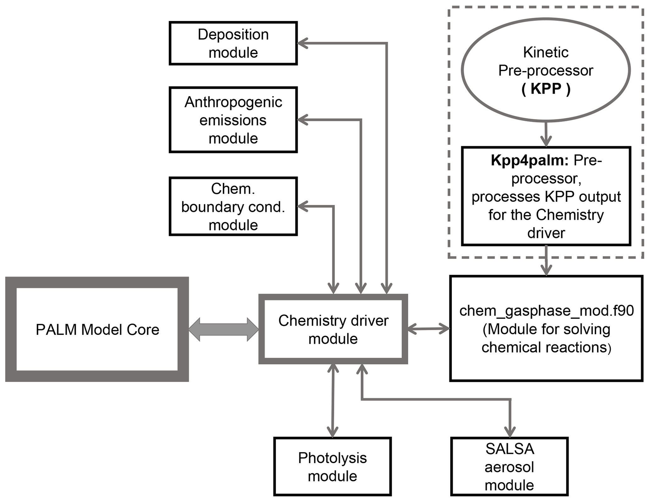
Figure 1 Schematic representation of the chemistry model (PALM-4U component) of the PALM model system. The arrows show interaction between the PALM model core, the chemistry driver module and sub-modules. The dashed box indicates the chemical preprocessor which generates subroutines to solve chemical reactions.

Depending on the need, a user can select a chemistry mechanism of different complexity. The Fortran code for the selected gas-phase chemistry mechanism is generated by a preprocessor based on KPP (Damian et al., 2002). The latter is described in more detail in Sect. 2.2.2. Besides chemical transformations in the gas phase and a simple photolysis parameterization (Sect. 2.2.3) the chemistry module includes dry deposition (Sect. 2.2.5), an interface to the aerosol module SALSA (Kurppa et al., 2019) (Sect. 2.2.4) and an option for anthropogenic emissions (Sect. 2.3).

2.2.1 Prognostic equations

When gas-phase chemistry is invoked, N additional prognostic equations are solved, with N being the number of variable compounds of the chemical reaction scheme. Except for the SGS flux terms, the overbar indicating filtered quantities is omitted to improve readability. The three-dimensional prognostic equation for an atmospheric pollutant then reads as follows:

$$\begin{array}{}\text{(1)}& \begin{array}{rl}{\displaystyle \frac{\partial c_n}{\partial t}}=& -{\displaystyle \frac{\mathrm{1}}{\mathit{\rho }}}{\displaystyle \frac{\partial \mathit{\rho }{u}_j{c}_n}{\partial x_j}}-{\displaystyle \frac{\mathrm{1}}{\mathit{\rho }}}{\displaystyle \frac{\partial \mathit{\rho }\stackrel{\mathrm{‾}}{u_j^{\prime \prime }{c}_n^{\prime \prime }}}{\partial x_j}}+{\left({\displaystyle \frac{\partial c_n}{\partial t}}\right)}_{\text{chem}}+{\mathrm{\Psi }}_n,\\ & \text{with}i,j\in (\mathrm{1},\mathrm{2},\mathrm{3}),\end{array}\end{array}$$

where c_n ($n=\mathrm{1},N$) is the concentration of the respective air constituent, which can be either a reactive or passive gas-phase species or an aerosol particulate matter compound. The term on the left-hand side is the total time derivative of the pollutant concentration. The first two terms on the right-hand side represent the explicitly resolved and the SGS transport of the scalar chemical quantity in x, y and z directions. A double prime indicates a SGS variable. The third term represents the change in concentration (c_n) of the trace gas n over time due to production and loss to chemical reactions, which can be described as follows:

$$\begin{array}{}\text{(2)}& ({\displaystyle \frac{\partial c_n}{\partial t}}{)}_{\mathrm{chem}}={\mathit{\varphi }}_n(c_{m\ne n})+{\mathit{\phi }}_n(c_{m\ne n})\cdot c_n,\end{array}$$

where ϕ_n and φ_n indicate the production and loss, respectively, of species n. For most of these production and loss reactions the rates are dependent on temperature and pressure. The last term in Eq. (1) (Ψ_n) stands for sources (i.e. emissions) and sinks (i.e. deposition and scavenging). The number of prognostic equations depends on the number of species included in the chemical mechanism, and it is determined automatically during the KPP preprocessing step (Sect. 2.2.2).

2.2.2 Gas-phase chemistry implementation

The Fortran subroutines for solving the chemical reactions of a given gas-phase chemistry mechanism are generated automatically with the KPP, version 2.2.3 (Damian et al., 2002; Sandu et al., 2003; Sandu and Sander, 2006). KPP creates the code from a list of chemical reactions that represent a certain chemical mechanism. Within the PALM environment, the subroutines with the integrator for the desired gas-phase chemistry mechanism are generated by a preprocessor named kpp4palm, which is based on the KP4 preprocessor (Jöckel et al., 2010). As a first step, kpp4palm starts the KPP preprocessor. As a second step, the code from KPP is transformed into a PALM subroutine. As described by Jöckel et al. (2010), the preprocessing also includes an optimization of the LU (lower–upper) decomposition of the sparse Jacobian of the ordinary differential equation system for the chemistry rate equations.

KPP offers a variety of numerical solvers for the system of coupled ordinary differential equations describing the chemical reactions. Tests comparing the performance of the Rosenbrock solvers implemented in KPP have shown that the use of the most simple Rosenbrock solver, Ros-2, did not lead to significantly different results than the use of the Rosenbrock solvers with higher orders (Sandu and Sander, 2006; Jöckel et al., 2010). Therefore, the Ros-2 solver was chosen as the default solver for the PALM-4U chemistry model.

The automatic code generation by kpp4palm and KPP allows for high flexibility in the choice of gas-phase chemical mechanisms and numerical solvers. Since the number of chemical compounds of a mechanism from KPP is used to determine the number of prognostic equations (Eq. 1), it is also possible to add prognostic equations for an arbitrary number of passive tracers by simply including reactions of the form A→A in the list of chemical reactions, which serves as input for KPP. For example, the passive tracer mechanism “passive” contains the following equations in the passive.eqn file:

{ 1.} PM10 = PM10 : 1.0 ;
{ 2.} PM25 = PM25 : 1.0 ;
(see Sects. S2–S9 of the Supplement for all .eqn files).

The chemistry model includes a number of ready-to-use chemical mechanisms summarized in Table 1. The first two mechanisms describe only one or two passive tracers which represent PM₁₀ and PM_2.5 (particulate matter with the aerodynamic diameter ≤10 and ≤2.5 µm, respectively) without any chemical transformations. As a representative of a “full” gas-phase mechanism, the well known Carbon Bond Mechanism 4 (CBM4) (Gery et al., 1989) is included. Although CBM4 has been replaced by the more detailed CB5 and CB6 mechanisms in the meantime, it is still applied in some models. The CBM4 mechanism was implemented in the PALM model, since – with 32 compounds – it is the smallest of the full mechanisms. Nevertheless, the comparatively large number of species precludes the use of the CBM4 mechanism for practical applications over larger domains. Therefore, we also included less computationally demanding mechanisms, such as the SMOG mechanism and its simplified version, the “SIMPLE” mechanism. By far, the photostationary equilibrium (PHSTAT mechanism) represents the most simple mechanism, consisting of only three species and two reactions. The latter two mechanisms are also supplied with an additional passive tracer which can be used to represent PM₁₀ (PHSTATP and SIMPLEP mechanisms). Three more mechanisms which can be used in combination with the sectional aerosol module SALSA (Kurppa et al., 2019) are described in Sect. 2.2.4.

Table 1 Description of built-in chemical mechanisms.

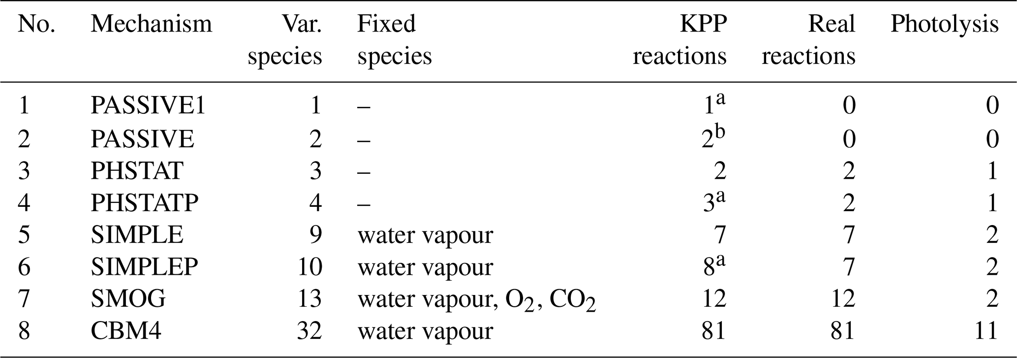
^a Includes one passive compound which is realized in the KPP environment by the “reaction” PM₁₀→ PM₁₀. ^b Includes passive compounds which are realized in the KPP environment by the “reactions” PM₁₀→ PM₁₀ and PM_2.5→ PM_2.5.

Two of the currently available mechanisms, SMOG and SIMPLE, include only major pollutants such as ozone (O₃), nitric oxide (NO), nitrogen dioxide (NO₂), carbon monoxide (CO), a highly simplified chemistry of volatile organic compounds (VOCs) and a very small number of products. For the convenience of the users, it is not required to run kpp4palm for the ready-to-use mechanisms (Table 1) as their Fortran subroutines are already supplied with PALM. Currently, PHSTATP is the default mechanism which will automatically be compiled with the rest of the PALM source code when the chemistry option is switched on. However, users can also add modified versions of the existing chemical mechanisms or define completely new mechanisms according to their specific needs.

2.2.3 Photolysis frequencies

The parameterization of the photolysis frequencies is adopted from the Master Chemical Mechanism (MCM) v3 according to Saunders et al. (2003). Photolysis frequencies are described as a function of the solar zenith angle ϑ and three parameters, which are specific for each photolysis reaction:

$$\begin{array}{}\text{(3)}& J=l\left(\cos \mathit{\vartheta }{)}^m\exp \right(-n\sec \mathit{\vartheta }).\end{array}$$

Values for l, m and n are given for the relevant photolysis reactions in Saunders et al. (2003) and on the MCM web page (http://mcm.leeds.ac.uk/MCM/parameters/photolysis_param.htt, last access: 12 July 2020). Currently only a simple parameterized photolysis scheme is available for photochemical reactions. More extensive photolysis schemes such as the Fast-J photolysis scheme (Wild et al., 2000) that are based on the radiative transfer modelling will be included in the future. These models will also make use of the shading due to buildings, which is already implemented for the shortwave radiation in the PALM-4U urban surface model but so far not for the simple photolysis scheme.

2.2.4 Coupling to SALSA aerosol module

The sectional aerosol module SALSA2.0 (Kokkola et al., 2008) has recently been implemented into PALM, and a detailed description is given in Kurppa et al. (2019). SALSA describes the aerosol number size distribution, aerosol chemical composition and aerosol dynamic processes. Currently, the full SALSA implementation in PALM includes the following chemical compounds in the particulate phase: sulfate (SO${}_{\mathrm{4}}^{\mathrm{2}+}$), organic carbon (OC), black carbon (BC), nitrate (NO${}_{\mathrm{3}}^{-}$), ammonium (NH${}_{\mathrm{4}}^{+}$), sea salt, dust and water (H₂O). Aerosol particles can grow by condensation and dissolution to liquid water of gaseous sulfuric acid (H₂SO₄), nitric acid (HNO₃), ammonia (NH₃), and semi- and non-volatile organics (SVOCs and NVOCs), which establishes a link between SALSA and the chemistry module.

SALSA is coupled to the gas-phase chemistry when the gas-phase compounds listed above (H₂SO₄, HNO₃, NH₃, SVOCs and NVOCs) are either included in the gas-phase chemistry scheme or are derived from prognostic variables of the gas-phase chemistry. Currently, PALM-4U includes three different mechanisms in which SALSA is coupled with the chemistry model. In the mechanisms “SALSAGAS” and “SALSA+PHSTAT”, H₂SO₄, HNO₃, NH₃, SVOCs and NVOCs are treated as passive compounds and are only transported within the gas-phase chemistry model, whereas in “SALSA+SIMPLE”, HNO₃ is formed by the reaction NO₂ + OH → HNO₃. Additionally, any of the other mechanisms given in Table 1 or any user-supplied mechanism can also be coupled to SALSA.

2.2.5 Deposition

Deposition is a major sink of atmospheric pollutant concentrations. Currently, only dry deposition processes are included as precipitation (leading to wet deposition of pollutants) is not yet included in PALM. For dry deposition, a resistance approach is taken where the exchange flux is the result of a concentration difference between atmosphere and earth surface and the resistance between them. Several pathways exist for this flux, each with its own resistance and concentration. The aerodynamic resistance depends mainly on the atmospheric stability. In PALM, it is calculated via MOST, based on roughness lengths for heat and momentum and the assumption of a constant flux layer between the surface and the first grid level.

For gases, the quasi-laminar layer resistance depends on the atmospheric conditions and diffusivity of the deposited gas, and it is calculated following Simpson et al. (2003). Finally, the surface (canopy) resistance for gases, which is the most challenging resistance to estimate due to the enormous diversity of surfaces, is calculated using the DEPAC module (Van Zanten et al., 2010). DEPAC is widely used in the flux modelling community (e.g. Manders et al., 2017; Sauter et al., 2016). The surface resistance parameterizations are different for different land use types defined in the model. In DEPAC, three deposition pathways for the surface resistance are taken into account:

• through the stomata

• through the external leaf surface

• through the soil.

DEPAC is extensively described in a technical report by Van Zanten et al. (2010). It also includes a compensation point for ammonia which is currently set to zero in PALM.

For the passive particulate matter in the chemistry model, the land-use-dependent deposition scheme of Zhang et al. (2001) has been implemented into PALM. The formulations have been chosen as they include an explicit dependence on aerosol size. For particulate matter, the deposition velocity is calculated by the gravitational settling or sedimentation velocity (mainly relevant for the larger particles), the aerodynamic resistance (see above), and the surface resistance. The sedimentation velocity mainly depends on particle properties, the gravitational acceleration and the viscosity coefficient of air. The formulation for the surface resistance is empirical with parameters that are based on a few field studies including the collection efficiencies for Brownian diffusion, impaction and interception, respectively, and a correction factor representing the fraction of particles that stick to the surface depending on the surface wetness. Further details can be found in Zhang et al. (2001).

2.3 Traffic emissions

The chemistry model of PALM-4U includes a module for reading gaseous and passive anthropogenic emission input from traffic sources and converting it to the appropriate format. These emission data can be provided in three possible levels of detail (LODs), depending on the amount of information available at the user's disposal. With LOD 0 (“PARAMETERIZED”, mode), traffic emissions are parameterized based on emission factors specific to particular street types. All street segments contained in the domain will be classified into “main” and “side” street segments. A mean surface emission flux tendency for each chemical species contained the active chemical mechanism, in kilograms per square metre per day, and will be provided together with a weighting factor for main- and side-street emissions in the PALM parameter file. Street type classification based on OpenStreetMap definitions (OpenStreetMap contributors, 2017) is to be included in the PALM static driver (Maronga et al., 2020). A diurnal profile derived from traffic counts is implemented to disaggregate total emissions into hourly intervals. Currently a default profile is applied to all species for main and side street segments, and details can be found in the online documentation for the PALM-4U chemistry model (https://palm.muk.uni-hannover.de/trac/wiki/doc, last access: 12 September 2020). Future plans include expansion of the LOD 0 emission model to accommodate further modes of anthropogenic emissions such as domestic heating. More detailed traffic emission data can be provided in gridded form in PALM-specific NetCDF files (Maronga et al., 2020). LOD 1 emissions are gridded annual emission data for each sector (e.g. industry, domestic heating, traffic), which will be temporally disaggregated using sector-specific standard time factors. With LOD 2, the user can introduce preprocessed gridded emission data that are already temporally disaggregated, e.g. in hourly intervals.

2.4 Initial and boundary conditions

Lateral boundary conditions for chemical compounds can be chosen in the same way as the lateral boundary condition for other scalars, e.g. potential temperature, being either cyclic conditions or non-cyclic (Maronga et al., 2020). In most urban applications, chemistry requires non-cyclic boundary conditions, because cyclic conditions lead to accumulation of pollutants to the modelling domain if pollutant emissions exist. As part of the PALM-4U components, nesting has been implemented to the chemistry module. In offline nesting, PALM can be coupled to a larger-scale (mesoscale, regional or global) model to provide dynamic boundary conditions for the meteorological variables as well as air pollutants. As larger-scale models do not fully resolve turbulence, a synthetic turbulence inflow generator has been introduced (Gronemeier et al., 2015).

Initial concentrations of primary compounds to control the chemistry model are controlled by the chemistry name list ”&chemistry_parameters” in the PALM parameter file. Options for prescribing initial conditions are available for both surface initial conditions and initial vertical profiles for the area or region of interest. There are no default initial concentrations and the user is responsible for providing these values based on, for example, the measured background concentration of primary chemical compounds for whom initial concentrations are defined. These primary compounds must be part of the applied chemical mechanism.

3 Chemistry model application

In order to demonstrate the ability of the chemistry implementation, we performed simulations for an entire daily cycle in a realistic urban environment and compared simulation results against observational data. To analyse the effect of different chemical mechanisms with different complexity on the resulting concentrations, we performed simulations with three chemical mechanisms and one passive case where only transport and dry deposition were considered.

3.1 Modelled episode and modelling domain

The model was run for 24 h from 00:00 to 24:00 UTC for 17 July 2017 (02:00 Central European Summer Time (CEST) 17 July 2017 to 02:00 CEST 18 July 2017) for a city quarter located around the Ernst-Reuter-Platz in Berlin, Germany. This particular day was chosen as it represents an “ideal” Berlin summer day with mostly clear sky, some scattered clouds in the morning after a partly cloudy night, and only a few passing clouds in the afternoon. The temperature ranged between 289 and 298 K with moderate winds predominantly from westerly direction. 17 July 2017 was a Monday; therefore, the diurnal cycle of the traffic emissions can be described as a typical weekday with relative maxima during the morning and evening rush hours.

Figure 2 shows the computational domain that covers an area of 6.71 km × 6.71 km (671 × 671 grid points) with a model top at 3.6 km above the surface. The horizontal grid spacing in x and y direction is 10 m. In the vertical, with 312 layers, the grid spacing is 10 m up to 2700 m, above which it increases by an expansion factor of 1.033 until the grid spacing in the z direction reaches 40.0 m.

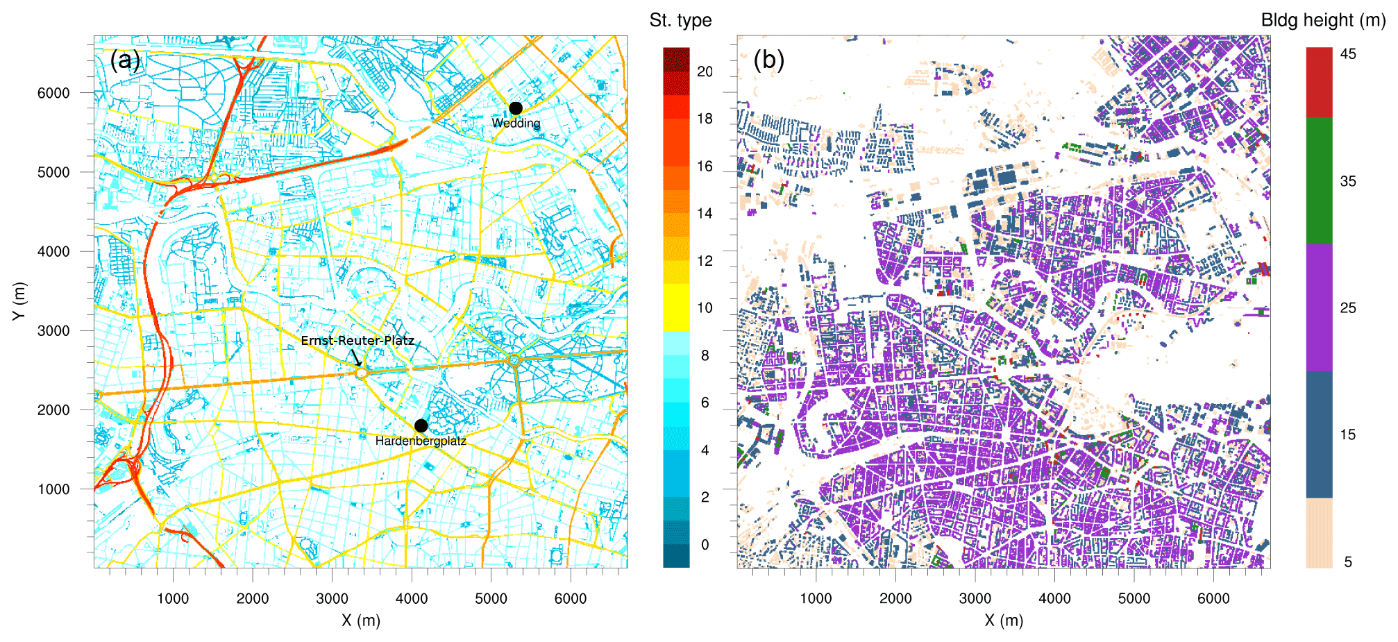
Figure 2 Simulation domain: (a) street type, (b) building height. The black dots show the location of the observational monitoring stations Wedding and Hardenbergplatz.

The topographic data with streets, buildings, water bodies, vegetation and other urban land surface features at a 10 m resolution have been processed for Berlin by the German Space Agency (DLR) (Heldens et al., 2020). The street types shown in Fig. 2a are based on OpenStreetMap (OpenStreetMap contributors, 2017). The model domain includes 13 types of one-way and two-way roads. The building height data are based on CityGML data from FIS Broker Berlin (Senatsverwaltung für Stadtentwicklung und Wohnen, 2020) (Fig. 2b). With the exception of 10 buildings with a height between 45 and 65 m and two buildings which are higher than 70 m, the building heights in the simulation domain are between 5 and 45 m.

The simulation domain contains five types of vegetation categories that include grass and shrubs of different height. Trees resolved by the canopy model are characterized by the three-dimensional leaf area density (LAD) per unit volume. For the model configuration used here, LAD is considered for a maximum height of up to 40 m above the ground and assumes values up to 3.1 m² m⁻³ with an average value of 0.44 m² m⁻³. Lake, river, pond and fountain categories are included in the domain for water types. Considering the urban surface, soil type of the entire domain is classified as “coarse”, whereas pavement types in the domain are defined with six different categories of asphalt, concrete and stones.

3.2 Observational data

In addition to routine observations of near-surface temperature, cloud cover, and wind speed and direction at the Berlin Tegel airport from the open-access Climate Data Center (CDC) of the German Weather Service (Deutscher Wetterdienst, 2020), we also analysed radiosonde data from Lindenberg (Oolman, 2017) and aerosol backscatter observations from a ceilometer for 16 and 17 July 2017 to understand the vertical structure of the atmosphere in the area of interest. Ceilometer observations of aerosol back-scatter profiles were performed on the roof of the Charlottenburg building of the Technical University of Berlin (52.5123^∘ N, 13.3279^∘ E) as part of the Urban Climate Observatory (UCO) operated by the Chair of Climatology at Technische Universität Berlin for long-term observations of atmospheric processes in cities (Scherer et al., 2019a; Wiegner et al., 2002) and contributed to the research program Urban Climate Under Change [UC]² (Scherer et al., 2019b). Mixing layer heights were derived from the aerosol backscatter signal according to Geiß et al. (2017).

Observations from radiosondes and ceilometers indicate strong showers during the previous days that resulted in a very well mixed (almost moist adiabatic) layer in the lower troposphere that lead to an almost constant potential temperature gradient above the inversion; therefore, there was no residual layer at midnight on 17 July, when the model was initialized for a 24 h run. The ceilometer observations for 17 July 2017 also did not show disturbances by clouds; the mixed-layer top, however, remained below 2000 m throughout the diurnal cycle.

The air quality measurements that are compared with the simulations are conducted at automated stations of the so-called BLUME network of the Berlin Department for the Environment, Transport and Climate Protection (Senate-Berlin, 2017). Two stations, Wedding and Hardenbergplatz (Fig. 2), are located within the model domain. The average height of the air quality sensors at both stations is 4 m above ground.

The roadside air quality station at Hardenbergplatz is located at a busy junction with high traffic flow and in close proximity to the train and bus stations. The station records only NO and NO₂. The height of the buildings in the vicinity of the station ranges from 10 to 30 m. The dense road network of small and big streets to the north, south and west of the station warrants transport of traffic-related pollutants towards Hardenbergplatz when the station is located downwind of these directions. To the north-east of the station is the Berlin Zoo and Tiergarten park that spread over 5.2 km². Thus, with a NE flow, the Hardenbergplatz air quality station would be downwind of the large vegetated area, and less anthropogenic pollutants would be advected to the station, although the concentration of biogenic volatile organic compounds (BVOCs) is expected to be larger.

The background air quality station of Wedding is located to the north in the outskirts of the city away from heavy traffic flow. Wedding air quality station records PM₁₀, NO, NO₂ and O₃. The city centre is located to the south of the station, so the station would likely record higher levels of NO_x and PM₁₀ during southerly flow. Both stations collect data every 5 min which are then averaged to hourly data and made available on the Senate department web pages (Senate-Berlin, 2017).

3.3 Model configuration and initialization

The PALM model system, version 6.0, revisions 4450 and 4601 (only for flux profiles of chemical compounds), has been used in this study. A multigrid scheme has been used to calculate pressure perturbations in the prognostic equations for momentum (Maronga et al., 2015), and a third-order Runge–Kutta scheme (Williamson, 1980) has been used for time integration. The advection of momentum and scalars was discretized by a fifth-order advection scheme by Wicker and Skamarock (Wicker and Skamarock, 2002). Following Skamarock (2006) and Skamarock and Klemp (2008), we employed a monotonic limiter for the advection of chemical species along the vertical direction in order to avoid unrealistically high concentrations within the poorly resolved cavities (e.g. courtyards represented by only a few grid points) which can occasionally occur due to stationary numerical oscillations near buildings. Rayleigh damping has been used above 2500 m in order to weaken the effect of gravity waves above the boundary-layer top.

The Rapid Radiative Transfer Model (RRTMG) (Clough et al., 2005), which is included in PALM, has been used to calculate radiation fluxes and radiation heating rates. Natural-type surfaces are treated by the land-surface model of PALM, while building surfaces are treated by the urban-surface model (Resler et al., 2017; Maronga et al., 2020). The surface roughness length is set according to the given building, vegetation, pavement and water types and based on the information from the static driver. The MOST then provides surface fluxes of momentum (shear stress) and scalar quantities (heat, moisture) at the lower boundary condition. The application of MOST assumptions on urban surfaces has not been thoroughly evaluated. However, similar studies, for example Letzel et al. (2008) and Gronemeier et al. (2020), show that LES results were in good agreement with wind-tunnel data representing an urban setting. Based on these findings, it is assumed that MOST is applicable in the simulated urban surface.

Three chemical mechanisms, namely PHSTAT, SMOG and CBM4, along with one no-reaction case have been applied (Table 1). The CBM4 (Gery et al., 1989) mechanism is the most complex mechanism currently included in PALM-4U. It includes VOC and HO_x (hydrogen oxide radicals), chemistry and formation of ozone, and further photochemical products. Assuming that the CBM4 is more accurate than the more simple mechanisms due to its more complete representation of atmospheric chemistry, the baseline simulation of this study was performed with CBM4. The SMOG photochemical mechanism was included for comparison as it contains a strongly simplified NO_x–HO_x–VOC chemistry with VOC just described by one single representative compound (Table 1). Due to a smaller number of species and reactions, the SMOG mechanism is much faster compared to the CBM4 mechanism. The objective of including the SMOG mechanism was to assess computational efficiency at the cost of accuracy of the description of the VOC chemistry. The most simple mechanism, PHSTAT, describes only the photostationary equilibrium between NO, NO₂ and O₃ and does not include any VOC chemistry or formation of any secondary compounds besides ozone. In a fourth experiment, the photostationary mechanism (PHSTAT) was applied with the gas-phase chemistry turned off; i.e. the chemical compounds were treated as passive tracers and only transport and dry deposition were allowed.

Only traffic emissions, which are parameterized depending on the street type (“PARAMETERIZED” option, LOD=0), were considered. Since the area of interest is in the inner part of the city with many major roads, and domestic heating emissions are neglectable in July, this restriction seems justified. The traffic emissions of the “PARAMETERIZED” option are based on emission factors derived from HBEFA (HandBook Emission FActors road transport; Hausberger and Matzer, 2017) and traffic counts provided by the Senate Department for the Environment, Transport and Climate Protection of Berlin. A mean surface emission of 4745 and 1326 $\mathrm{\mu }\mathrm{mol}{\mathrm{m}}^{-\mathrm{2}}{\mathrm{d}}^{-\mathrm{1}}$ is applied for NO and NO₂, respectively, and weights of 1.667 for main streets and 0.334 for side streets are applied for the current study. Considering the diurnal cycle of emissions a typical temporal profile of traffic emissions (see Sect. S1 of the Supplement), with maxima at 08:00 and 18:00–19:00 CEST based on traffic counts at Ernst-Reuter-Platz, was applied.

As initial conditions profiles of θ, q, u, v and w, soil moisture and soil temperature were obtained from the output of the operational mesoscale weather prediction model COSMO-DE/D2 (COnsortium for Small-scale MOdelling; Baldauf et al., 2011) for 17 July 2017. The INIFOR tool was used to prepare these initial conditions in a format that can be read by PALM (Kadasch et al., 2020). The initial profiles of pollutant concentration are based on the mean observed near-surface concentrations of NO, NO₂ and O₃ from the stations of the BLUME network (Sect. 3.2). Initial concentrations of NO, NO₂ and O₃ above 495 m were set to 0.0, 2.0 and 40.0 ppb respectively. Considering the strong impact of traffic emissions on local pollutant concentrations, all grid points of the model domain were initialized with identical pollutant profiles.

At the lateral boundaries, cyclic boundary conditions are applied for the velocity components, θ, q and the chemical compounds. The application of cyclic boundary conditions may be justified by low variability in wind direction with prevailing westerly winds throughout the major part of 17 July 2017 and the large extent of the urban area upwind of the model domain. One main reason for not applying boundary conditions from COSMO-DE/D2 was that it requires a very large fetch to develop turbulence, as turbulence quantities are not supplied by the boundary conditions from the mesoscale COSMO-DE/D2 simulation. Furthermore, chemistry fields for the lateral boundaries were not available from COSMO-DE/D2. Thus, cyclic boundary conditions were applied that ensure cyclic inflow of meteorological and chemistry variables that left the domain from the opposite lateral boundary. Therefore, a continuous inflow and outflow of pollutants in and out of the simulation domain is assumed. This is reasonable, as the simulation domain is located in the middle of a large highly urbanized area.

At the bottom boundary, a Dirichlet condition is applied to flow, θ and q, whereas a Neumann condition is applied to e, p and chemical compounds. Moreover, a canopy drag coefficient C_d = 0.3 has been applied while the roughness is specified internally depending on vegetation type. At the top boundary, Dirichlet boundary conditions are applied to flow and p only, and initial gradient is applied to θ while Neumann boundary conditions are applied to q and chemical compounds.

4 Results and discussion

The results of the chemistry model simulations are presented for 20 h from 03:00 UTC (05:00 CEST) to 23:00 UTC (01:00 CEST 18 July 2017). All plots and data in this case study are presented in CEST. The simulation output was exported to file every 10 min as instantaneous values and every 30 min as temporal averages. Since observational data are available in hourly averaged data, we used the 30 min averaged model data for comparison with observations. For all other plots we used instantaneous data.

4.1 Meteorology

Figure 3 shows vertical profiles of potential temperature, mixing ratio, wind speed and wind direction over the diurnal cycle. The profiles of potential temperature indicate a vertically well mixed boundary layer during daytime, evolving from approximately 500 m at 07:00 CEST to more than 2300 m at 21:00 CEST, while in the evening hours the near-surface layer stabilizes. The mixed-layer depth agrees fairly well with the observed values from ceilometer measurements (horizontal bars in Fig. 3a), except for the late afternoon and evening hours, where the modelled boundary-layer depth is over-predicted by up to 15 %. This can have various causes; e.g. in our simulations we neglected larger-scale processes such as subsidence or mesoscale advection. The wind comes from westerly directions at a mean wind speeds of about 6–9 m s⁻¹ within the mixed layer.

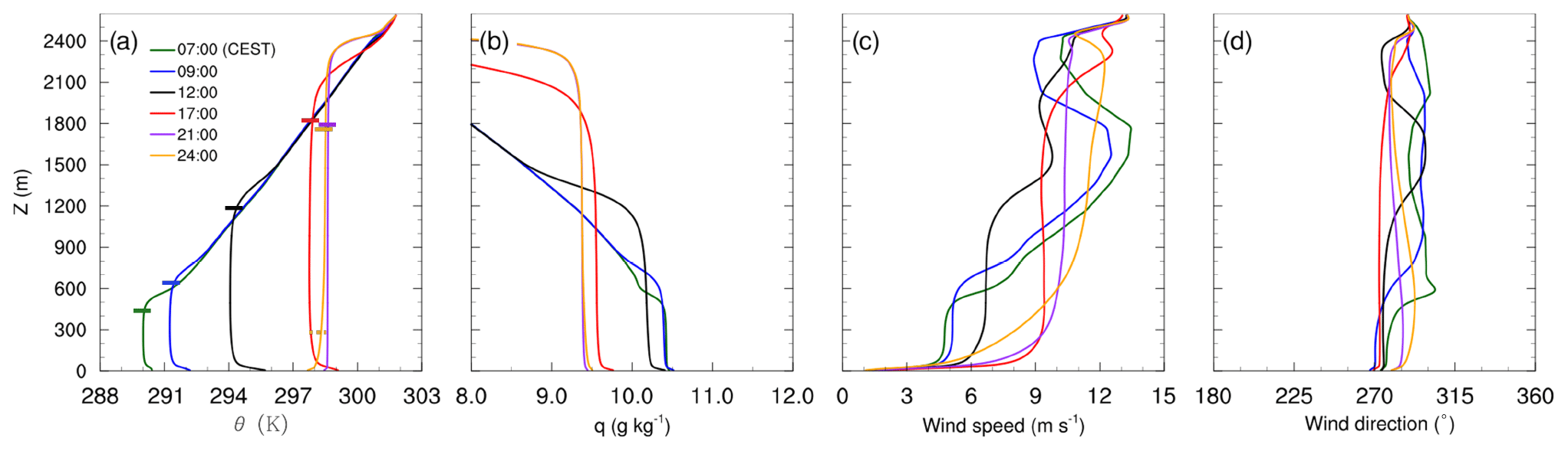
Figure 3 Vertical profiles of (a) potential temperature, (b) mixing ratio, (c) wind speed and (d) wind direction, at different times from morning to midnight on 17 July 2017. The horizontal bars in (a) indicate the boundary-layer height derived from ceilometer observations.

4.2 Vertical mixing of NO₂ and O₃

Figure 4 shows mean profiles of concentrations and vertical fluxes of NO, NO₂, O₃ and CO for the selected times of the diurnal cycle on 17 July 2017, simulated with the CBM4 mechanism. Profiles and fluxes of CO are added to represent transport characteristics of passive species. Positive fluxes with a negative vertical gradient can be observed for NO and NO₂, indicating net upward transport of the respective compounds from the surface towards higher levels during the entire diurnal cycle. The emitted NO from traffic sources oxidized to NO₂ by reaction with the available O₃:

$$\begin{array}{}\text{(R1)}& \mathrm{NO}+{\mathrm{O}}_{\mathrm{3}}\to {\mathrm{NO}}_{\mathrm{2}}+{\mathrm{O}}_{\mathrm{2}}.\end{array}$$

This leads to an increase in NO₂ and a decrease in O₃ within the boundary layer. As indicated by Fig. 4g the growth of the boundary layer after sunrise leads to downward transport of O₃ since ozone concentrations in the residual layer are higher than within the mixed layer. At the same time, photolysis of NO₂ (Reaction R2) and photochemical formation of O₃ (Reaction R3) by VOC chemistry retained and slightly increased the O₃ concentration within the boundary layer as well as in the residual layer.

$$\begin{array}{}\text{(R2)}& {\displaystyle }{\mathrm{NO}}_{\mathrm{2}}+h\mathit{\nu }\to \mathrm{NO}+\mathrm{O}{(}^{\mathrm{3}}\mathrm{P})\text{(R3)}& {\displaystyle }{\mathrm{O}}_{\mathrm{2}}+\mathrm{O}{(}^{\mathrm{3}}\mathrm{P})+M\to {\mathrm{O}}_{\mathrm{3}}+M\end{array}$$

Near-surface concentrations of NO are 1 to 2 ppb higher than the remaining mixed layer throughout the diurnal course. At 09:00 CEST, owing to emissions from traffic sources, the NO concentration increases from 3 to 5 ppb in the first few metres above the surface then evenly dilutes in the shallow mixed layer and stabilizes with a mixing ratio of 3 ppb. Besides the high NO_x emissions in the morning hours, this increase can also be attributed to the onset of NO₂ photolysis (Reaction R2). During the rest of the day, NO concentrations gradually reduces, mostly due to dilution by vertical mixing during further growth of the mixed layer as well as the fast reaction with O₃ (Reaction R1). The NO concentrations above the inversion are much lower and mostly influenced by the background levels thus making NO vertical flux positive (Fig. 4e) showing upward transport of NO.

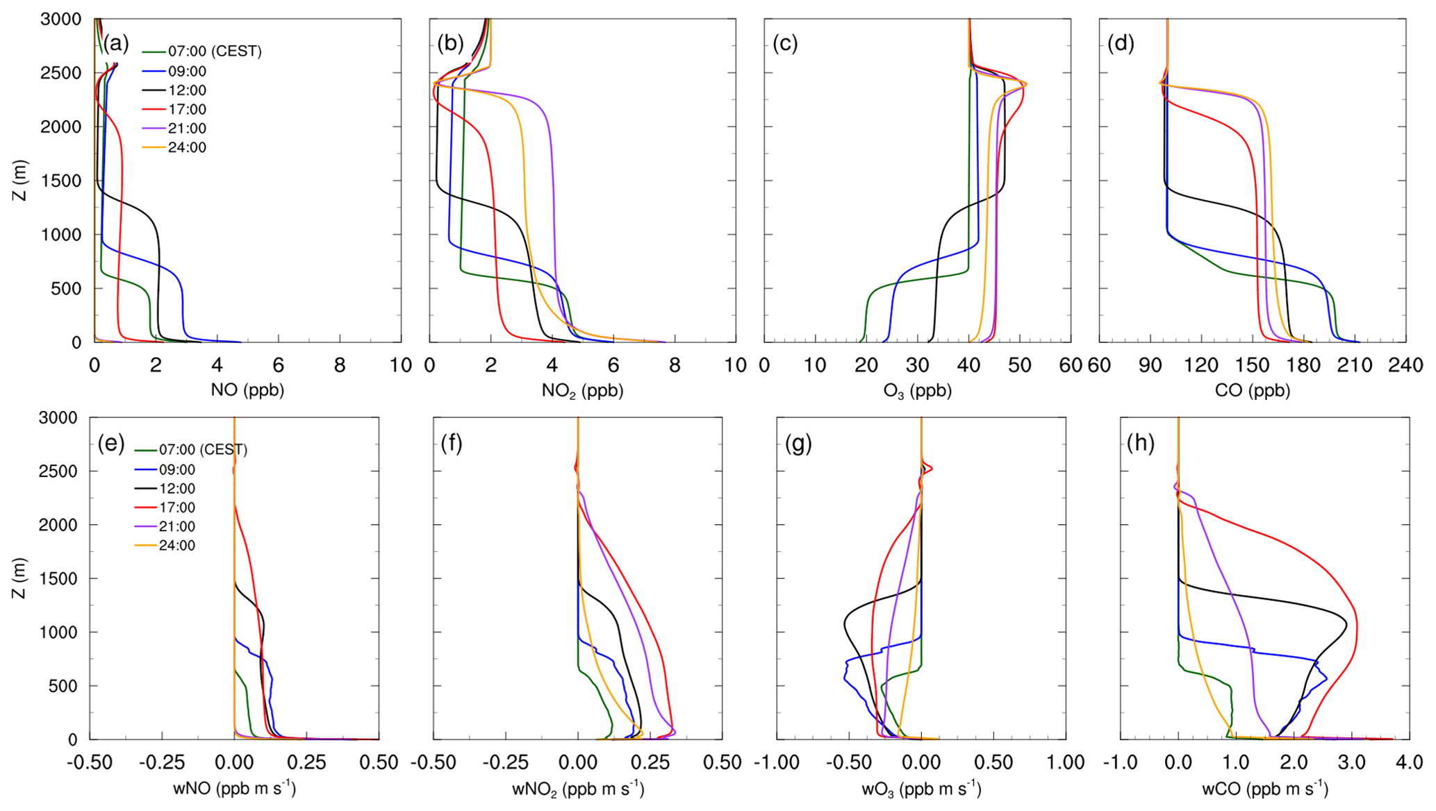
Figure 4 Mean vertical profiles of species concentration for (a) NO, (b) NO₂, (c) O₃ and (d) CO, as well as their total vertical fluxes (e–h) over the diurnal cycle on 17 July 2017, simulated with the CBM4 mechanism.

Unlike NO, the NO₂ concentration profiles in Fig. 4b show only small differences in the morning hours (07:00 and 09:00 CEST). In the afternoon (12:00 and 17:00 CEST) when the convection is stronger, the NO₂ concentration is the lowest due to the combined effect of upward vertical mixing indicated by Fig. 4f and photolysis of NO₂ (Reaction R2).

Reactions (R1)–(R3) between NO, NO₂ and O₃ do not result in a net gain of O₃ unless additional NO₂ is supplied (e.g. primary NO₂ from traffic emissions) and O₃ is formed by Reactions (R2) and (R3). However, OH radical chain reactions of VOCs result in the formation of excess NO₂ (Reactions R4 and R5) and thus O(³P) (Reaction R2), which results in a net O₃ gain (Cao et al., 2019). In a schematic form, the formation of NO₂ due to VOC oxidation can be summarized by

$$\begin{array}{}\text{(R4)}& {\displaystyle }\mathrm{OH}+\mathrm{RH}+{\mathrm{O}}_{\mathrm{2}}\to {\mathrm{RO}}_{\mathrm{2}},\text{(R5)}& {\displaystyle }{\mathrm{RO}}_{\mathrm{2}}+\mathrm{NO}\to \mathrm{RO}+{\mathrm{NO}}_{\mathrm{2}},\end{array}$$

where RH stands for any explicitly described or lumped non-methane hydrocarbon and RO₂ represents any organic peroxy radical.

In addition to Reaction (R3), the O₃ levels within the mixed layer are also replenished through down-welling from above the inversion during the day, which is evident from the negative flux profiles of O₃ (Fig. 4g). As a result O₃ concentration gradually increased from 18 ppb at 07:00 CEST to 43 ppb at 17:00 CEST.

In the evening hours (21:00 CEST onward), the NO concentration is reduced to 1 ppb near the surface while it is completely removed from the residual layer. In the reduced (no) solar radiation, NO₂ photolysis (Reaction R2) slows down (stops), whereas emission and a limited Reaction (R1) reaction (because of very low available NO) favours an increase in the NO₂ mixing ratio. This resulted in the highest near-surface NO₂ concentrations at 24:00 CEST in the nocturnal stable layer. In the well mixed residual layer above, the NO₂ concentration at 24:00 CEST is up to 1 ppb lower than NO₂ concentrations at 21:00 CEST. Ozone is also reduced to 3 ppb at 24:00 CEST but remains well mixed in the residual layer above the shallow nocturnal stable boundary layer. Carbon monoxide has been added to the analysis as a proxy to passive species (Fig. 4d). In the morning hours, the concentration is highest, then it gradually decreases due to turbulent mixing in the rapidly growing mixed layer and partly due to dry deposition.

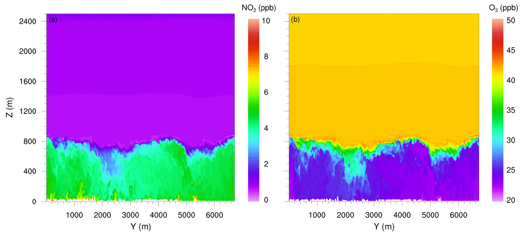
Figure 5 shows YZ vertical cross sections at Hardenbergplatz for NO₂ and O₃. Turbulence and the growth of the mixed-layer height caused downward vertical mixing and O₃ entrainment near the boundary-layer top that resulted in increase in O₃ concentration as well as in a decrease in NO₂ concentrations to 2.0 ppb. Near the ground, the NO₂ concentration is still of the order of 10 ppb. At the top of the boundary layer, the concentration of OH and HO₂ were higher than in the surrounding areas, which indicates active NO_x–VOC–O₃ chemistry in the turbulent entrainment zone.

Figure 5 YZ vertical cross sections of NO₂ and O₃ (drawn through Hardenbergplatz, Fig. 2a), simulated with the CBM4 mechanism at 09:00 CEST on 17 July 2017.

4.3 Spatial distribution of pollutants

The spatial distribution of NO₂ and O₃ concentrations 5 m above the surface (Fig. 6) are discussed for 09:00 and 21:00 CEST as simulated with the CBM4 mechanism. The concentrations of NO_x, aldehyde and hydrocarbon species (not shown), which are emitted by road traffic, were high in the morning and evening hours due to stable conditions and high emissions.

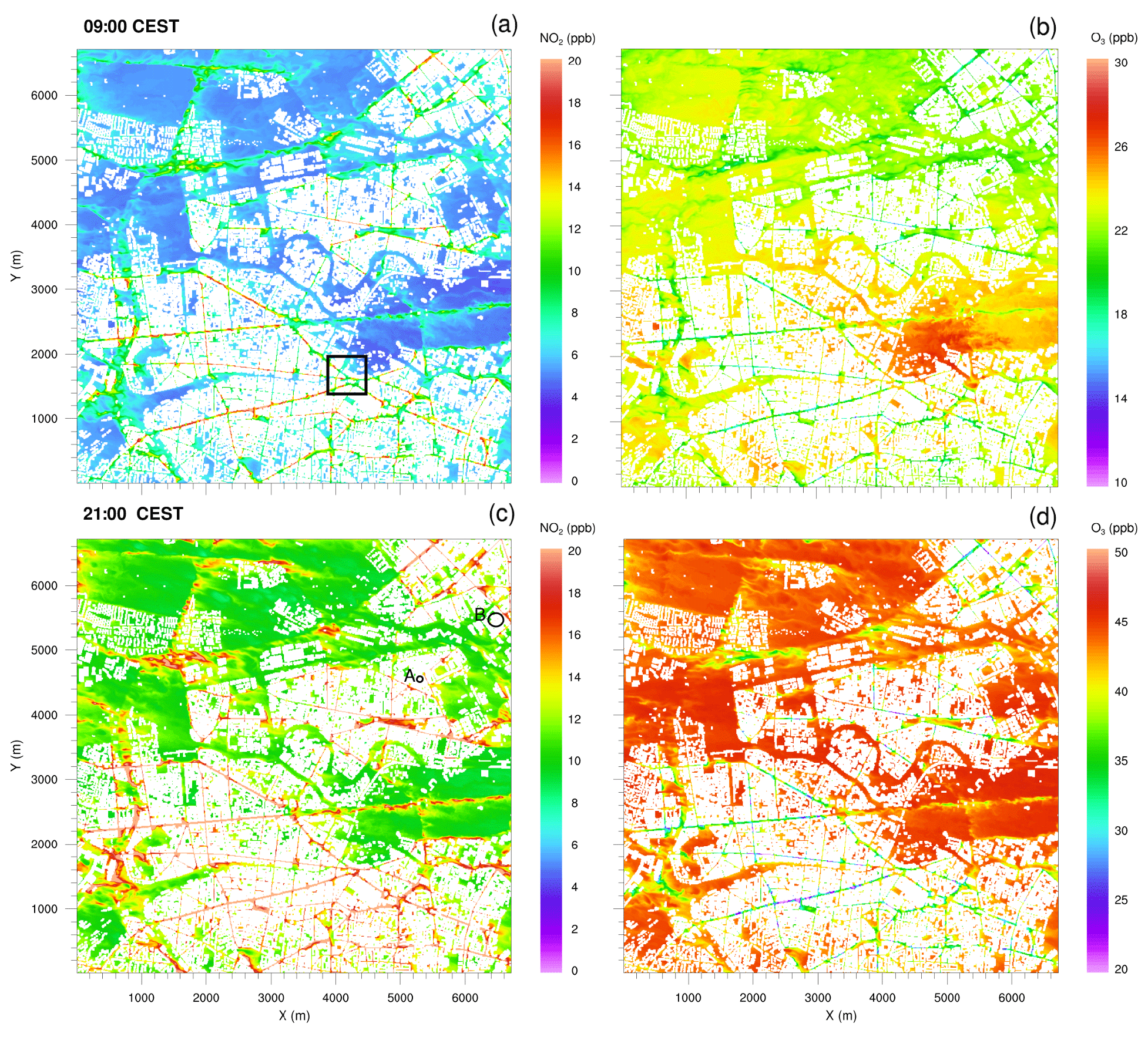
Figure 6 Horizontal cross sections of near-surface NO₂ and O₃ concentrations at 09:00 and 21:00 CEST on 17 July 2017, simulated with the CBM4 mechanism. The black square in (a) indicates the location of the small domain presented in Fig. 7. Locations A and B in plot (c) indicates isolated street canyons plotted in Fig. 8.

Most of the high NO₂ concentrations in the morning hours (Fig. 6a) are predicted in the street canyons in the southern part of the simulation domain, where numerous buildings with a height of approximately 20 m are present (see Fig. 2a). In the street canyons of this area, wind speeds of less than 2 m s⁻¹ were simulated below 20 m, while wind speeds were almost twice as high over the open areas in the northern part of the model domain (not shown). Therefore, emitted NO_x is more diluted by advection over the open areas. Furthermore, in the morning hours compared to the open spaces, vertical mixing and transport in the street canyons is inhibited mainly due to delayed heating of the ground, which is attributed to the shading of the surrounding buildings. Therefore, O₃ is predominantly titrated by Reaction (R1) (Fig. 6b) over the road network reducing its concentration to the order of 20 ppb, while over open spaces and vegetation (especially the southern part of the Tiergarten) a slightly higher O₃ mixing ratio (27 ppb) is found. The initial O₃ values near the surface were set to 10 ppb increasing to 40 ppb around 500 m above the surface. A higher concentration of O₃ (30 ppb) near the surface in the open spaces indicates strong vertical mixing and downward transport of O₃ in the morning hours of the day. In the evening, however, the NO₂ distribution is somewhat more uniform over the entire road network (Fig. 6c). This is attributed to emissions from traffic with reduced or absent photolysis of NO₂ (Reaction R2) and titration of O₃. Under the low-wind conditions below 50 m, ventilation is reduced and leads to an increase in NO₂ over street crossings and main and side roads. Consequently, the NO₂ concentration increased by 30 % in the evening hours over roads and adjacent paved areas, whereas over the vegetated areas (grass, crops, shrubs and trees), NO₂ concentrations were around 5 ppb in the morning hours and reached up to 10 ppb in the evening hours. The daytime NO_x–O₃–VOC chemistry resulted in elevated O₃ levels which increased by more than 100 % as compared to the morning concentrations, mostly due to photochemical production of O₃ (Reactions R2 and R3) during daytime. In the evening hours (Fig. 6d), O₃ is largely titrated by Reaction (R1) over the road network. In certain sections of the street canyons where micro-meteorological conditions are more favourable, O₃ levels decreased to 20 ppb. However, in the open spaces and over vegetation with very low NO, the O₃ concentration is of the order of 50 ppb.

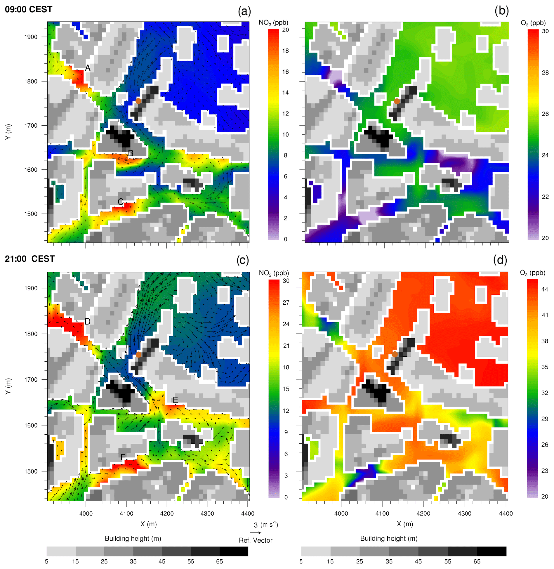
Figure 7 Near-surface NO₂ and O₃ concentrations in the street canyons near Hardenbergplatz, simulated with the CBM4 mechanism at 09:00 and 21:00 CEST on 17 July 2017. The wind vectors in (a) and (c) show horizontal wind speed 5 m above the surface. The filled brown dot in (a) indicates the location of Hardenbergplatz air quality station. Grey shading indicates building height.

To provide an overview of the pollutant dispersion at the street level, a small section of the model domain (500 × 500 m) in the Hardenbergplatz area has been analysed (Fig. 7). This small urban section is characterized by a typical urban environment with streets, paved areas, buildings with varying heights and some vegetated areas of the Tiergarten located to the north-east. The dispersion of air pollutants in a street canyon generally depends on the aspect ratio (ratio of building height to street width) and rate at which the street exchanges air vertically with the above roof-level atmosphere and laterally with connecting streets (N'Riain et al., 1998). Figure 7 shows the dispersion and chemical transformation of NO₂ and O₃ in the street canyons and surrounding areas. The vegetated area of the Tiergarten north-east of the domain has relatively high O₃ levels and small NO₂ concentrations, which is attributed to the low NO concentrations over the vegetation that lead to reduced O₃ titration (Reaction R1). The model has emissions only from traffic sources, and therefore availability of the primary species other than roads depends upon the dispersion of the primary chemical compounds such as NO. In the street canyons, O₃ is titrated by NO by Reaction (R1) resulting in production of NO₂.

In the morning hours, NO₂ concentration increases in some sections of the street canyons (locations A, B and C in Fig. 7a) which are located to the west/southwest of the tall buildings and thus lie under the shade of the building structures. Due to the particular street geometry, and flow dynamics above the urban canopy, these sections also experience weak wind conditions. The elevated NO₂ concentrations are due to later onset of the turbulence and vertical exchange caused by reduced solar radiation in the shade of the buildings. This results in increased residence time of NO and O₃ due to very localized calm or near-calm conditions in the street canyons. The daytime NO–O₃–VOC chemistry significantly increases O₃ concentration. In the evening hours when photolysis of NO₂ is again decreasing, the NO_x and O₃ chemistry was mostly controlled by Reaction (R1) and wind speed in the street canyons. The street sections (locations D, E and F in Fig. 7c) with low wind and calm conditions experience relatively elevated NO₂ and low O₃ levels as under calm conditions NO has enough residence time to titrate O₃ and thus contribute towards increased NO₂ concentrations. Streets with stronger winds over the open spaces (train tracks, Tiergarten area) experience lower than average NO₂ levels.

At some locations, PALM simulated unrealistically high NO₂ concentrations. Figure 8 shows time series plots along with xy cross section of the street canyons (in the inset) where the model simulated high NO₂ concentrations at location A and B as indicated in Fig. 6c. We selected four grid points at location A and five random grid points from the discontinued street canyon at location B. During the day, NO₂ concentrations remain up to 50 ppb; however, after 18:00 CEST, the NO₂ concentrations increase rapidly at both locations. By 21:00 CEST, NO₂ concentration at location A is of the order of 75 ppb (Fig. 8a), whereas, at location B, NO₂ levels ranges between 65 and 90 ppb (Fig. 8b). At 01:00 CEST, the NO₂ concentration at both locations A and B reaches 150 and 275 ppb respectively.

Figure 8 Time series plots from (a) four individual grid points with high concentrations at location A, and (b) five randomly selected grid points from the isolated street canyon at location B as indicated in Fig. 6c. The inset shows the close-up view of these isolated cavities at location A and B at 21:00 CEST on 17 July 2017. Colours of the curves in the time series plots are randomly selected and has no relevance to the shading of the inset plots.

Due to a relatively coarse grid resolution of 10 m, as applied in this study, street canyons are partly only resolved by one or two grid points, and sometimes enclosed cavities occur. Within such geometries the flow is only poorly resolved by the numerical grid, which means that the bulk of the transport is parameterized by the subgrid model. However, as the subgrid TKE is also very low in such narrow canyons or cavities (not shown), the total vertical transport is rather low, especially in the evening hours when the surface layer stabilizes. If, however, surface emissions are still high within such street canyons, chemical compounds can accumulate and will not be sufficiently transported away. Here, we emphasize that such accumulation of compounds cannot be observed with a higher grid resolution of 1–2 m where street canyons are sufficiently resolved by the numerical grid.

4.4 Comparison of the three chemical mechanisms

Figure 9 shows the time–height plots of NO₂ and O₃ at Hardenbergplatz. All six plots exhibit a clear signal of gradual boundary-layer growth from morning to evening. The concentrations of both NO₂ and O₃ differ between the three chemical mechanisms which can be attributed to their different levels of complexity and different description of the reactions resulting in either photochemical equilibrium or net formation of ozone and other photochemical products.

Due to the photostationary state, there is no net O₃ production in the PHSTAT mechanism (Fig. 9a and b). In the morning hours, despite Reaction (R1) that consumed most of the NO, the NO₂ concentration is slightly reduced to 7 ppb by 07:00 CEST compared to its initial near-surface background levels of 10 ppb. The small drop in NO₂ concentration is attributed to the mixing of NO₂ within the shallow mixed layer reaching 500 m in depth. Titration of O₃ by NO consequently reduces O₃ concentrations to 15 ppb. After 07:00 CEST, photodissociation leads to a decrease in NO₂ to very low levels (2–4 ppb) 50 m above the surface. However, NO₂ concentration remains of the order of 6 to 7 ppb close to the surface due to emissions from roads and NO_x–VOC–HO_x chemistry. Consequently, O₃ concentration peaks between 13:00 and 18:00 CEST by Reaction (R3). Above the rapidly growing mixed layer, the background concentration remained 2 and 40 ppb for NO₂ and O₃ respectively. In the evening and night-time emissions from traffic, suppression of NO₂ photolysis (Reaction R2) and a slow Reaction (R1) reaction increases NO₂ concentrations near the surface up to 20 ppb, while O₃ concentration is suppressed to less than 15 ppb due primarily to Reaction R1. Above the stable nocturnal boundary layer the NO₂ is well mixed in the near-neutral residual layer with a concentration of around 10 ppb, while due to absence of NO in the residual layer, and downward transport of background O₃ concentration through the entrainment zone, the O₃ concentration increases by 30 ppb in the residual layer.

Photolysis of NO₂, daytime NO_x–VOC chemistry in the case of the SMOG (Fig. 9c and d) and CBM4 (Fig. 9e and f) mechanisms result in O_x production and increased O₃ levels during the day with maximum values in the afternoon. Various VOC reactions form peroxy radicals that oxidize NO to NO₂, and other nitrate products help increase O₃ concentration, whereas CO, CO₂ and HNO₃ act as atmospheric sinks to aldehydes, NO_x and O₃ in SMOG.

In the CBM4 mechanism NO₂ levels are reduced as much as 40 % between 12:00 and 19:00 CEST, whereas the O₃ concentration increases by almost the same percentage. Since no reactions leading to a net production of O₃ are considered for the photostationary state (PHSTAT mechanism), the maximum ozone concentration is determined by the photolysis of NO₂ and is therefore lower than for the SMOG and CBM4 mechanisms.

The interaction of NO_x with O₃ chemistry is more pronounced near the surface. In all three mechanisms, a gradual decay of O₃ is found near the surface in the evening (after 20:00 CEST). During the daytime, especially and in particular in the morning hours, entrainment of O₃ from the residual layer during the growth of the boundary layer contributes to the increase in the O₃ concentration in the mixed layer. In the evening, after the collapse of the mixed layer, a well mixed residual layer with near-uniform pollutant concentration can be found above the shallow, stably stratified nocturnal boundary layer. Although behaviour of NO_x and O₃ is essentially the same in all three mechanisms, the difference is more evident in the CBM4 mechanism because we see a more pronounced diurnal course of O₃ in CBM4.

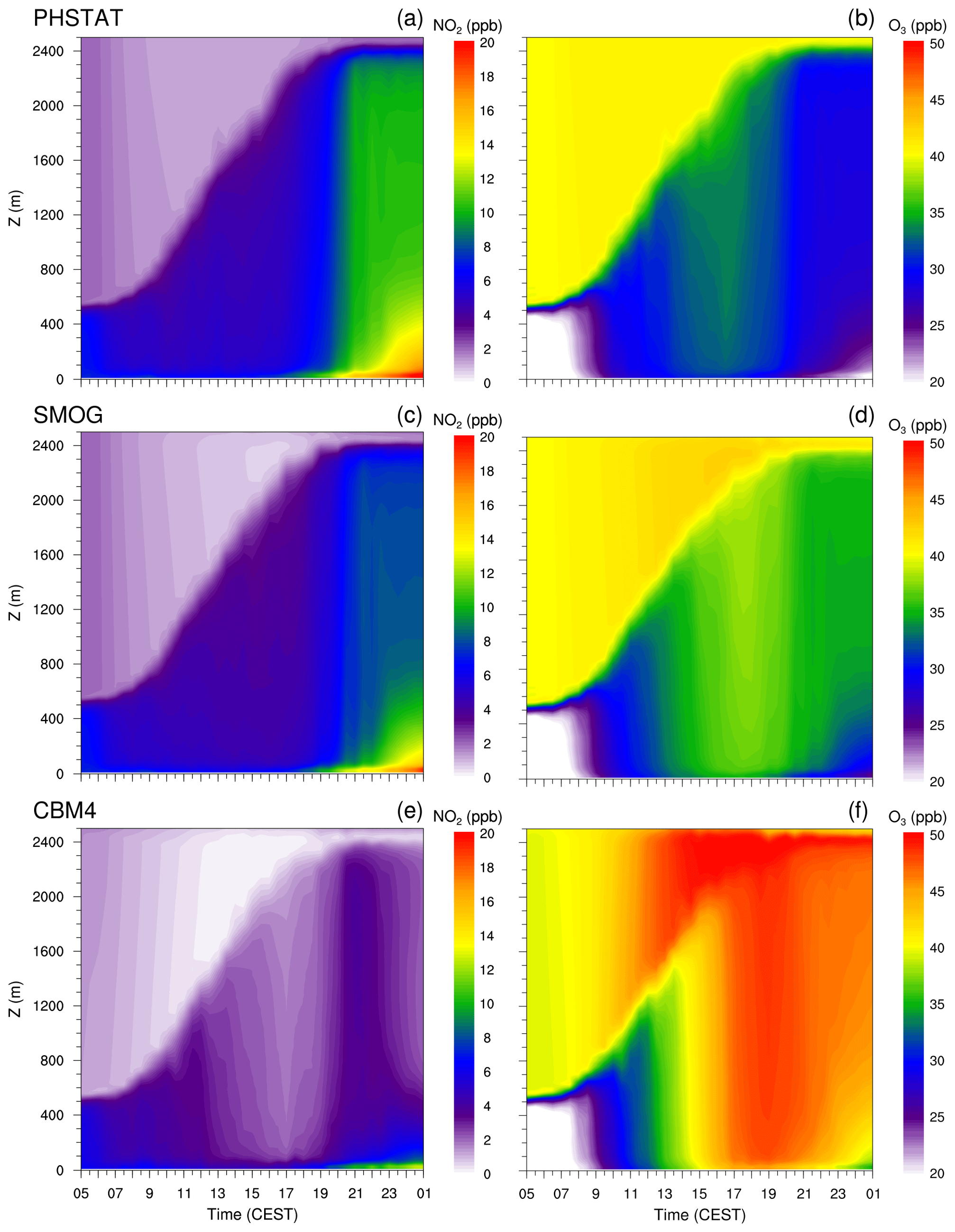
Figure 9 Time–height cross section of half-hourly averaged NO₂, and O₃ concentrations simulated with the PHSTAT, SMOG and CBM4 mechanisms from 05:00 CEST (17 July 2017) to 01:00 CEST (18 July 2017) at Hardenbergplatz. The left column (a, c, e) shows NO₂, and the right column (b, d, f) shows O₃ concentration.

4.5 Comparison of pollutant concentrations with observations

The observation data from Wedding and Hardenbergplatz are compared with the mean concentrations of the modelled NO, NO₂ and O₃ from five points in the vicinity of the Wedding and Hardenbergplatz stations (Fig. 10). Error bars indicate standard deviation at every hour in the time series data from the five points. Ozone is not measured at Hardenbergplatz, and therefore the time series curve of the observed O₃ is not included in Fig. 10, and the analysis at Hardenbergplatz is restricted to NO and NO₂ species only.

The three mechanisms (PHSTAT, SMOG and CBM4) are able to reproduce the diurnal cycle of NO, NO₂ and O₃ with reasonable accuracy. The CBM4 mechanism shows a more pronounced diurnal course than SMOG and PHSTAT. The timing of the maximum ozone concentration is reproduced much better in the CBM4 mechanism than the SMOG and PHSTAT mechanisms. Since the PHSTAT mechanism does not include any net O₃ formation, the maximum O₃ concentration occurs at the time of maximum solar elevation. However, the SMOG and the CBM4 mechanisms include photochemical ozone production which leads to higher maximum ozone concentrations. A shift of the maximum ozone concentration from local noon to later afternoon is in agreement with observations. Due to a more detailed description of NO_x–VOC–HO_x chemistry, this process is described more realistically for the CBM4 mechanism than for the SMOG mechanism. All three mechanisms failed to realistically simulate evening peaks in NO_x (NO and NO₂) concentrations and the corresponding low O₃ concentrations. This could possibly be related to the overly slow cooling of the surface as described earlier, which results in less pronounced stable layer near the ground after sunset. A reason could be that the observed decrease in the wind speed to values below 1 m s⁻¹ between 22:00 and 24:00 h CEST could not be reproduced by the model due to the application of cyclic boundary conditions. Since O₃ is inversely related to NO_x, the underestimated NO_x concentration in the evening leads to reduced titration of O₃ and therefore results in higher levels of O₃. Another reason for the bias of the model could be due to the uncertainties in the description of the traffic emissions. We utilized only parameterized traffic emissions, which may under-represent the emissions at the considered locations in the evening hours.

The no-reaction case only contains transport and dry deposition of NO_x. Without chemical reactions, NO continues to increase, which is primarily due to the lack of chemical sinks in combination with the application of cyclic boundary conditions. In contrast to the cases with chemical reactions, NO₂ is lower than NO since there is no conversion of NO to NO₂. Despite titration by NO, a very slow increase in the near-surface O₃ in the morning hours can be attributed to the downward mixing from the residual layer during the growth of the mixed layer.

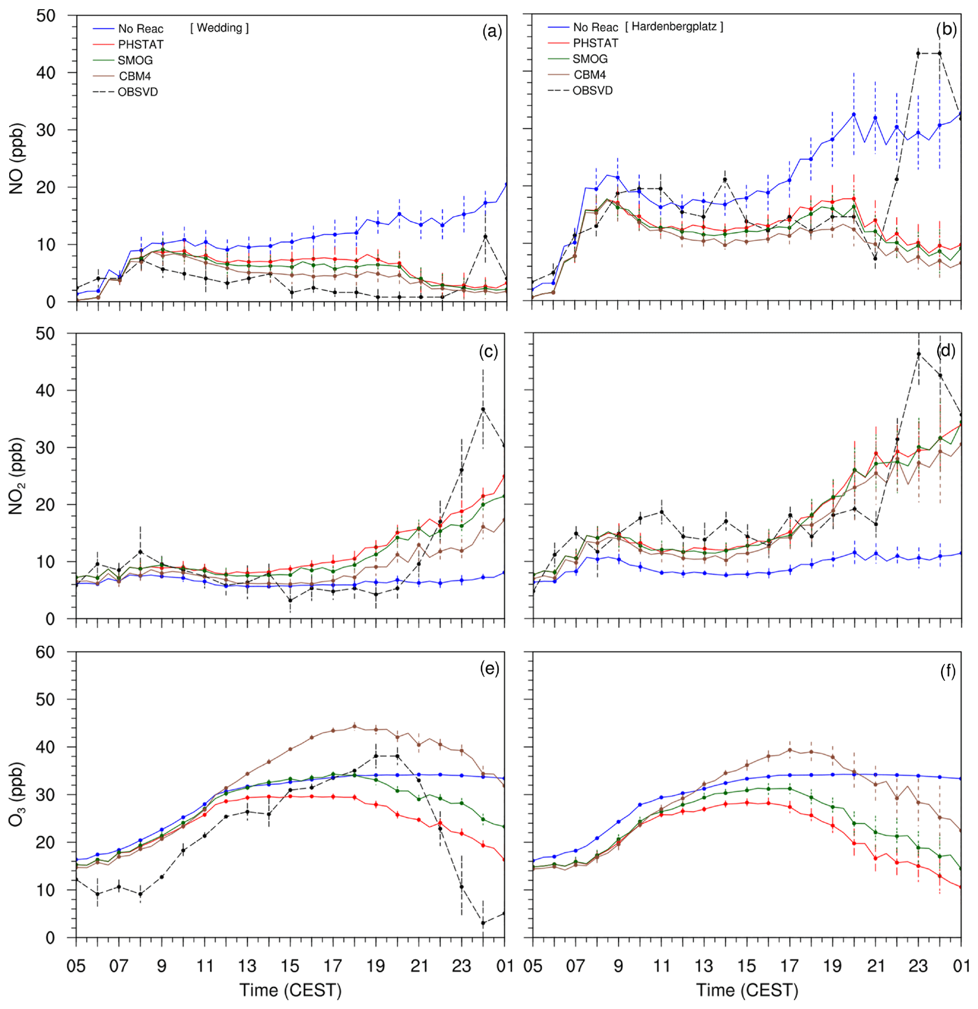
Figure 10 Time series plots of the near-surface NO, NO₂ and O₃ concentrations from four mechanisms (NO-REAC, PHSTAT, SMOG, CBM4) and observations from 05:00 CEST (17 July) to 01:00 CEST (18 July 2017). The left column (a, c, e) shows time series from Wedding, and the right column (b, d, f) shows time series plots from Hardenbergplatz.

4.6 Computational efficiency

Chemistry models are known for utilizing a relatively large amount of computational power, and the same applies to the chemistry model implemented in the PALM model. This is mainly due to the complexity in solving the stiff Jacobian matrix because reaction rates of chemical species vary greatly, which leads to a time-step much smaller than meteorological parameters, and therefore the computation speed of the entire system is largely affected. The simulation of the chemical reactions can take as much as 90 % of the total computational time in the calculation of an online-coupled simulation (Cao et al., 2019). The computation time of chemistry increases with the increasing number of the chemical compounds and the number of chemical reactions in a given chemical mechanism. Table 2 shows a comparison of the increase in computational time for four chemical mechanisms relative to the corresponding meteorology-only simulation on two different high-performance computing systems and two different single-domain extents.

For case A, simulations were performed for a domain with 96 × 96 × 320 grid points and dx= dy= dz=10 m. The model domain for the case A simulations is a smaller part of the model domain shown in Fig. 2 with the centre located at the Ernst-Reuter-Platz. The simulations for case A are performed on the Karlsruhe Institute of Technology (IMK-IFU) cluster on 96 CPUs of the Intel Ivy Bridge processors. Case B consists of the simulations which are discussed in the previous sections. The configuration and domain size is described in Sect. 3.1. These simulations were performed at the North-German Super computing Alliance (HLRN) (Berlin) with 784 Intel Cascade Lake Platinum 9242 CPUs (CLX-AP) on standard96 partition. Both cases have been integrated for 24 h. Due to the limited computational resources, the “transp. only” option (i.e. no-reaction; species used as passive scalars only) for all mechanisms was applied only for case A. As for “transp. only” simulations for case B, only the single run for the PHSTAT mechanism from Sect. 4.5 was available.

The results show a significant increase in the computational cost relative to the meteorology-only simulation for the same model domain. The comparison of “transp. only” and “(full)” for case A (Table 2) shows that the transport of additional scalar variables is even more expensive compared to the computation of the chemical transformation. While the increase in computational costs for the transport increases linearly with the number of compounds, this is not the case for computation of chemical conversion. As described by Verwer et al. (1999) the efficiency of the applied Rosenbrock solver increases with the increasing size of the chemical mechanism. Comparison of the “transp. only” option of case B with “full” suggests that for the PHSTAT mechanism the computational expense for the transport of the additional scalars is almost the same as for the computation of the chemical transformation. Although the “transp. only” simulation for case B was only performed for PHSTAT, presumably the relative computational expense for “transp. only” and “full” for the other mechanisms would not be much different for case A and case B.

Table 2 Increase in computational expense of a simulation with the PASSIVE, PHSTAT, SMOG and CBM4 mechanisms relative to a simulation without chemistry. For case A, the simulations were for a model domain with 96 × 96 × 320 grid points and a grid width of 10 m. For case B, the simulations were performed for a model domain with 671 × 671 × 312 grid points and a grid width of 10 m. Both runs were made in scalar mode for one full day. The term “transp. only” indicates the relative expense when solely the transport of the considered compounds is calculated and chemical transformation is switched off, and “full” refers to the run with transport as well as chemical transformations.

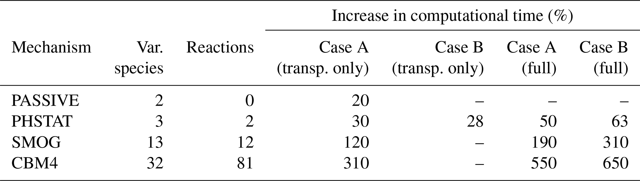
Given the highest number of chemical compounds and consequently the number of reactions, the CBM4 mechanism is the most resource-intensive of all mechanisms, which is 5.5 times more expensive than a plain meteorology-only simulation for the small domain (case A), and 6.5 times more expensive for the large domain simulation (case B). Considering the high computational resource requirement of chemistry-coupled LES simulations, it is important to invest extra efforts in the design of the simulation and selection of the appropriate chemical mechanisms.

5 Concluding remarks

We have outlined the structure and important features of a chemistry model that has been added to the PALM model system 6.0 as part of PALM-4U (PALM for urban applications) components and coupled to the PALM model core. PALM model system 6.0 is the first LES model that can simulate chemical transformation, advection and deposition of air pollutants for larger and realistically shaped urban areas (Maronga et al., 2019). PALM 6.0, offers many advanced features, which were not included in other LES models, for example self-nesting and large-scale forcing for chemical species, flexibility of choice in selection and generation of gas-phase chemistry mechanisms with the KPP preprocessor, and the availability of the chemistry model in both RANS and LES mode.

The results of the presented case study demonstrate the ability of the chemistry model to predict photochemical reactions, along with advection and deposition of pollutants. The difference between reactive and non-reactive cases clearly indicates that invoking reactive chemistry is of critical importance to accurately predict pollutant concentrations at the microscale. The simulated concentrations follow the observed diurnal cycle of the pollutants. However, the weak agreement warrants an improvement in the description of the parameterized emissions, large-scale forcing and model resolution.

Especially with coarse grid resolution some street canyons are only poorly resolved by the numerical grid, occasionally leading to the situation that street canyons are only one grid point wide or isolated cavities occur. However, within such enclosed cavities the flow is only poorly resolved too, meaning that the total transport of energy and matter is only small, especially under stable conditions. Emissions at such enclosed geometries may result in unrealistically high concentrations of primary compounds like NO_x. With increasing grid resolution such narrow street canyons will be better represented on the numerical grid, lowering the risk that high emissions coincide with regions where the flow is only poorly resolved. Hence, especially for lower grid resolutions, we recommend carefully inspecting the concentration output to treat high concentrations in the data analysis adequately.

The computational cost of the chemistry coupled simulations largely depends on the number of chemical compounds and the number of chemical reactions. The transport of additional scalar variables are found to be more expensive than the computation of the chemical transformation. Considering the high computational demand of chemistry coupled LES simulations, it is important that users should be careful in the choice of the chemistry mechanism for their specific needs.

Although the maximum ozone concentration and the time of its occurrence is somewhat better reproduced with the CBM4 mechanism than with the SMOG mechanism, it is difficult to give a final recommendation for an optimum mechanism. For some applications – in particular for low-VOC conditions – SMOG or even the photostationary equilibrium may be sufficient while for other simulations the application of the CBM4 mechanism is simply not possible due to its high computational demand. However, when using strongly condensed mechanisms like SMOG with only one single VOC compound, the user must always keep in mind that the simulated concentrations of ozone and further oxidation products depend strongly on the rate constant for the reaction of this single lumped VOC with OH. As already elaborated by Middleton et al. (1990), the reactivity of the lumped VOC depends on the VOC mix and therefore on the local emissions. On the other hand, CBM4 is still too simple for investigations with a special focus on VOC chemistry or a prediction of semi- and non-volatile organics, which are required for the SALSA aerosol model. In this case more detailed or advanced chemistry mechanisms than CBM4 may be required, which can be easily added since the flexible configuration of the chemistry in the PALM model allows the easy implementation of new mechanisms.

The chemistry model implemented in PALM is under continuous development: new features are being added and current features are being improved both in terms of efficiency and accuracy. We plan to further extend the model chemistry by implementing an advanced biogenic volatile organic compound (BVOC) emission scheme, emission parameterization of residential heating, biogenic pollen emission, transport and deposition scheme. Moreover, the chemistry model will be further improved by including a simplified scheme for ultra-fine particles in addition to the one already implemented in SALSA (Kurppa et al., 2019). Additionally, chemical boundary conditions, road-resuspension processes, wet-deposition processes of air pollutants and a photolysis parameterization based on shading information will be implemented in the chemistry model. We also plan to provide a more complex and detailed chemistry for the RANS mode, while for the LES mode, currently only strongly simplified mechanisms are possible due to computational constraints.