the Creative Commons Attribution 4.0 License.
the Creative Commons Attribution 4.0 License.
 | 25 Feb 2021
Global storm tide modeling with ADCIRC v55: unstructured mesh design and performance
Damrongsak Wirasaet
Keith J. Roberts
Joannes J. Westerink
This paper details and tests numerical improvements to the ADvanced CIRCulation (ADCIRC) model, a widely used finite-element method shallow-water equation solver, to more accurately and efficiently model global storm tides with seamless local mesh refinement in storm landfall locations. The sensitivity to global unstructured mesh design was investigated using automatically generated triangular meshes with a global minimum element size (MinEle) that ranged from 1.5 to 6 km. We demonstrate that refining resolution based on topographic seabed gradients and employing a MinEle less than 3 km are important for the global accuracy of the simulated astronomical tide. Our recommended global mesh design (MinEle = 1.5 km) based on these results was locally refined down to two separate MinEle values (500 and 150 m) at the coastal landfall locations of two intense storms (Hurricane Katrina and Super Typhoon Haiyan) to demonstrate the model's capability for coastal storm tide simulations and to test the sensitivity to local mesh refinement. Simulated maximum storm tide elevations closely follow the lower envelope of observed high-water marks (HWMs) measured near the coast. In general, peak storm tide elevations along the open coast are decreased, and the timing of the peak occurs later with local coastal mesh refinement. However, this mesh refinement only has a significant positive impact on HWM errors in straits and inlets narrower than the MinEle and in bays and lakes separated from the ocean by these passages. Lastly, we demonstrate that the computational performance of the new numerical treatment is 1 to 2 orders of magnitude faster than studies using previous ADCIRC versions because gravity-wave-based stability constraints are removed, allowing for larger computational time steps.
- Article
(17087 KB) - Full-text XML
-
Supplement
(6171 KB) - BibTeX
- EndNote


Extreme coastal sea levels and flooding driven by storms and tsunamis can be accurately modeled by the shallow-water equations (SWEs). The SWEs are often numerically solved by discretizing the continuous equations using unstructured meshes with either finite-volume methods (FVMs) or finite-element methods (FEMs). These unstructured meshes can efficiently model the large range in length scales associated with physical processes that occur in the deep ocean to the nearshore region (e.g., Chen et al., 2003; Westerink et al., 2008; Zhang et al., 2016; Le Bars et al., 2016; Fringer et al., 2019), although many difficulties for large-scale ocean general circulation modeling remain (Danilov, 2013). However, for barotropic flows that are largely responsible for extreme coastal sea levels, the capability to model the global scale concurrently with local coastal scales resolved in sufficient detail so that emergency planning and engineering decisions can be made is well within reach. Furthermore, barotropic global storm tide models can be used as components of Earth system models to analyze risks posed by the long-term response of extreme sea level and coastal flooding to climate change in far greater detail than is currently possible (Bouwer, 2018; Vousdoukas et al., 2018).
A key practical advantage of ocean models discretized using FEMs compared to FVMs is that they are usually less sensitive to mesh quality (e.g., element skewness). Specifically, ocean models discretized using FVMs often use staggered C-grid arrangements (e.g., Delft-FM) that have strict grid orthogonality requirements for numerical accuracy (Danilov, 2013; Fringer et al., 2019). The orthogonal requirement makes mesh generation over wide areas with fractal shoreline boundaries an arduous task that is difficult to automate, although progress has been made (Herzfeld et al., 2020; Hoch et al., 2020). Despite the difficulties, the FVM Delft-FM-based (FM: flexible mesh) Global Tide and Surge Model (GTSM) (Verlaan et al., 2015) has been meticulously developed and widely used to generate reanalysis datasets, describe historical trends, and make projections of extreme sea levels (Muis et al., 2016; Vousdoukas et al., 2018; Muis et al., 2019; Dullaart et al., 2019). Note that these previous studies neglected the contributions to extreme sea levels by short waves that can drive a significant regional setup (e.g., Fortunato et al., 2017). The minimum (coastal) resolution of GTSM has been historically limited to ∼5 km but was recently upgraded to 2.5 km (1.25 km in Europe) (Dullaart et al., 2019).
In the absence of constraints on orthogonality or element skewness, automatically generating unstructured triangular meshes on the spherical Earth that accurately conform to the coastline and cover a wide range of spatial sales (O(10 m)–O(10 km)) is completely realizable (Legrand et al., 2000; Gorman et al., 2006; Lambrechts et al., 2008; Roberts et al., 2019a). In one study, automatically generated ocean-basin-scale meshes with variable element sizes (50 m to 10 km) were used to conduct dozens of numerically stable FEM simulation experiments without mesh hand edits or numerical limiters (Roberts et al., 2019b). The ability of FEM models to handle rapid transitions in mesh element sizes combined with the ease of mesh generation with modern technologies (e.g., Roberts et al., 2019a) enables the application of seamless local refinement directly into the global mesh where required, potentially on the fly based on atmospheric and ocean conditions that indicate a risk of coastal flooding.
This study conducts a systematic analysis of unstructured mesh design in order to assess and demonstrate the capabilities of global storm tide modeling using FEMs across multi-resolution scales spanning from the deep ocean to the nearshore coastal ocean environment. One outcome of this study is a recommendation of unstructured triangular-element mesh design of the global ocean that represents the barotropic physics with high fidelity using relatively few elements (Sect. 3.1). Moreover, we test the added benefit of seamless local refinement in storm landfall regions to the simulation of storm tides (Sect. 3.2). Mesh generation is handled by the OceanMesh2D toolbox (Roberts et al., 2019a), which provides the tools to explore the effects of mesh design in a systematic way. For simulation we use the ADvanced CIRCulation (ADCIRC) model (Luettich and Westerink, 2004), which has been updated in this study for efficiency and to correctly model the SWEs on the sphere (Sect. 2.1); it is set for release as version 55. Section 3.3 summarizes the timing results with ADCIRC v55, highlighting its computational efficiency using a semi-implicit time integration scheme. In summary, this study aims to (1) highlight improvements to the treatment of the governing equations and implicit time integration in the new version of ADCIRC (v55) and (2) explore the effects of unstructured mesh design on storm tide solutions.
2.1 Global finite-element storm tide model
The ADCIRC storm tide model used in this study is an FEM solver that has been extensively used for detailed hurricane inundation studies at local and regional scales (e.g., Westerink et al., 2008; Bunya et al., 2010; Hope et al., 2013), as well as for an operational storm tide forecast model run by the US National Oceanic and Atmospheric Administration (NOAA) (Funakoshi et al., 2011; Vinogradov et al., 2017). ADCIRC solves the SWEs that are composed of primitive continuity and non-conservative depth-averaged momentum equations under astronomical and atmospherical forcing. After neglecting radial velocity terms, we formulate these equations in spherical coordinates as follows (Kolar et al., 1994):
where ζ is the free surface, U and V are the depth-averaged zonal and meridional velocities, respectively, H is the total water depth, t is time, λ is longitude, ϕ is latitude, R is the radius of the Earth, and ρ0 is the reference density of water. Additional terms are defined as follows.
Here, ps is the surface air pressure, g is the gravitational acceleration, η is the summation of the equilibrium tidal potential and self-attraction and loading (SAL) tide (Ray, 1998), Ω is the angular speed of the Earth, R is the radius of the spherical Earth, CD is the quadratic wind drag coefficient computed using the Garratt (1977) drag law, ρs is the density of air at the ocean's surface, Uw and Vw are the zonal and meridional 10 m wind velocities, respectively, and Cf is the quadratic bottom friction coefficient. 𝒞 is the internal wave drag tensor that accounts for the energy conversion from barotropic to baroclinic modes through internal tide generation in the deep ocean (Garrett and Kunze, 2007). Here, the local generation formulation is used (see Pringle et al., 2018a, b), in which Cit is a global tuning coefficient, Nb and Nm are the seabed and depth-averaged buoyancy frequencies, respectively, ω is set to the angular frequency of the M2 tide, and ∇hλ and ∇hϕ are the zonal and meridional topographic gradients, respectively. Last, τ denotes the lateral stress tensor, with νt denoting the lateral mixing coefficient. The components τλϕ and τϕλ can be chosen to be either symmetric or non-symmetric as desired (Dresback et al., 2005). For this study we choose the symmetric option.
To properly compute the governing equations on the spherical Earth in the FEM framework used by ADCIRC, we have upgraded the model formulation and code as detailed in Sect. S1 in the Supplement. This involves rotating the Earth so that the pole singularity is removed (Sect. S1.3) before applying a rectilinear mapping projection to transform the governing equations into a Cartesian form with spherically based corrections to the spatial derivatives (Sect. S1.1). Here, the continuity equation is multiplied by a factor dependent on the choice of cylindrical projection used (e.g., Mercator) to produce a conservative form that leads to discrete mass conservation and stability (see Hervouet, 2007; Castro et al., 2018) (Sect. S1.2). The stability of the ADCIRC solution scheme (Sect. S1.4) was analyzed in one-dimensional linear form (Sect. S1.5) to provide guidelines for the choice of numerical parameters that can be chosen to remove the gravity-wave-based (Courant–Friedrichs–Lewy, CFL) constraint. The validity of this analysis in the 2D nonlinear form has been demonstrated through the numerical simulations presented in this paper. With a semi-implicit time integration scheme, the computational time step permitted is larger than the CFL constraint and as a result facilitates computationally efficient global simulations on meshes that have nominal minimum resolutions of 150 m–1.5 km (see Sect. 3.3 for details). Hereafter, the updated code in this study refers to the new release, ADCIRC v55. Solutions using the uncorrected model formulation are referred to by the previous version, ADCIRC v54.
2.2 Unstructured triangular mesh generation on the Earth
The global unstructured meshes in this study are generated automatically using scripts with version 3.0.0 of OceanMesh2D (Roberts et al., 2019a; Pringle and Roberts, 2020). No post-processing hand edits of any mesh were necessary to obtain numerically stable simulations. Meshes are built in the stereographic projection centered at the North Pole to maintain angle conformity on the sphere and have the elements wrap around the Earth seamlessly, including an element placed over the North Pole (Lambrechts et al., 2008). Interested readers can execute Example_7_Global.m contained within the OceanMesh2D package to generate their own global mesh in a similar fashion.
Mesh design is handled through mesh size (resolution distribution) functions that are defined on a regular structured grid, usually that of the topo-bathymetric digital elevation model (DEM). In this study we use functions based on the distance to shoreline, bathymetric depths, and topographic gradients (see Table 1 for definitions). The final mesh size function is found by taking the minimum of all individual functions and applying nominal minimum and maximum mesh resolution bounds as well as an element-to-element gradation limiter to bound the transition rate (Roberts et al., 2019a). The effects of the individual mesh size functions and bounds on barotropic tides in a regional model have been previously detailed in Roberts et al. (2019b), which we use to guide our experiments exploring mesh design.
Table 1The mesh size functions used to spatially distribute element resolution, ER. The variable parameter in each function is indicated by α.
ds: shortest distance to the shoreline, : period of the M2 tidal wave, h: still-water depth, h*: low-pass-filtered h, in which ℱlp(L) is the low-pass filter with cutoff length L.
Additionally, this study makes use of the OceanMesh2D “plus” function, which seamlessly merges two arbitrary meshes together, keeping the finer resolution in the overlapping region. We use this function to apply local mesh refinement to a global mesh in storm-affected coastal regions to better resolve semi-enclosed bays and lakes, inlets, back bays, channels, and other small-scale shoreline geometries.
2.3 Experimental design
The experimental design we pursue is composed of two distinct steps, both with the purpose of maximizing model efficiency while maintaining a threshold of accuracy. First, we begin with a mesh design that we assume is a highly refined discretization of the Earth in a global sense and systematically relax the mesh size parameters to reduce the total number of mesh vertices while trying to minimize any negative impacts on global model accuracy. Second, we take the resulting recommended global mesh design from the previous step and apply local mesh refinement to increase the coastal resolution in the storm landfalling region and potentially improve local model accuracy.
2.3.1 Step 1: global mesh design
In this step, three mesh size function parameters (MinEle, TLS, and FL) are systematically relaxed to coarsen an initially highly refined discretization of the Earth, termed the reference (Ref) mesh design (see Table 2). In the Ref design, MinEle is set to 1.5 km, mainly due to practical constraints (e.g., computer memory usage when generating a global mesh in OceanMesh2D), and MaxEle is set to 25 km because common global meteorological products are defined on ∼25 km grids (aliasing errors in interpolation of the meteorological input data become an issue when a coarser grid is considered). The parameters WL, D, and G are considered fixed for all mesh designs based on prior knowledge that ∼30 elements per wavelength (WL) is sufficient for global ocean tides (Greenberg et al., 2007), and an element-to-element gradation limit and distance expansion rate (G and D) as high as 0.35 are tolerable as long as the TLS mesh size function is applied (Roberts et al., 2019b). As a note, the FL parameter is used in the construction of the TLS mesh size function to filter out small-scale topographic features (see Table 1) that are potentially unimportant to the local barotropic physics, thus disregarding those features for the application of higher resolution. This study is the first to test the effect of the FL parameter in detail. In each mesh design perturbation, only one of the three parameters is changed, while the other parameters are kept identical to those used in the Ref design. For illustration, the spatial distribution of the resolution of the Ref design compared to the TLS-B design is shown in Fig. 1.
Table 2Summary of the global mesh designs. Each row is separate and made up of three mesh designs for each variable mesh size function parameter, in addition to the Ref mesh design, which is the same for each row.


Figure 1Mesh resolution distribution (defined as the minimum connected element edge length for a mesh vertex) for two global mesh designs: (a) Ref and (b) TLS-B (see Table 2).
To assess the effect on the global model accuracy as the mesh designs are coarsened, we compare simulated astronomical tidal solutions to the data-assimilated TPXO9-Atlas. We focus on astronomical tides in this step because they can be reduced to a series of harmonic constituents of well-defined frequencies to make systematic global comparisons (Roberts et al., 2019b; Pringle et al., 2018a). The TPXO9-Atlas is the latest release of the TPXO satellite-assimilated tidal model (Egbert and Erofeeva, 2002). According to Egbert and Erofeeva (2019), the mean M2 RMSEt (tidal root mean square error; see Appendix A for definition) is 0.5 cm versus Stammer et al. (2014) deep-ocean tide gauges and ∼3 cm versus Stammer et al. (2014) shallow-water tide gauges. The metric of comparison between mesh designs is based on the area-weighted empirical cumulative distribution function (ECDF) of the five-constituent total tidal root mean square error, RMSEt|tot (see Appendix A). The two-sample Kolmogorov–Smirnov test statistic, K (see Appendix A), is used to provide a single metric of comparison between two ECDF curves.
2.3.2 Step 2: local mesh refinement
In this step, the recommended global mesh design from Step 1 (Sect. 2.3.1) is used but with additional patches of high resolution (local mesh refinement) near the landfall location of two storm events. We choose to focus on a particularly significant historical storm event from each of the Atlantic and Pacific ocean basins where tropical cyclones most commonly occur.
-
The first is the western North Atlantic – Hurricane Katrina, 23–31 August 2005. The most severe impact of storm-tide-induced coastal flooding occurred in the Louisiana–Mississippi region of the USA in the northern Gulf of Mexico (URS Group Inc, 2006a, b).
-
The second is the western Pacific – Super Typhoon Haiyan, 3–11 November 2013. The most severe impact of storm-tide-induced coastal flooding occurred in and around Tacloban, Philippines, at the back end of the Leyte Gulf (Mori et al., 2014).
Local mesh refinement is achieved by using OceanMesh2D to automatically merge a locally generated mesh for each landfall region (Louisiana–Mississippi: Fig. 2, Leyte Gulf: Fig. 3) into the global mesh. Two local meshes are generated for each region: one with MinEle = 500 m and another with MinEle = 150 m. The other mesh size function parameters are kept the same as the global mesh design, except that G and D are reduced to 0.25 because the mesh quality generated in the local domain was considered too low with a value of 0.35. Furthermore, the locally refined meshes only add an additional 0.5 %–3 % to the total mesh vertex count compared to the original global mesh design; thus, there is limited motivation to use higher values of G and D to try and save on mesh vertices in the local refinement region.
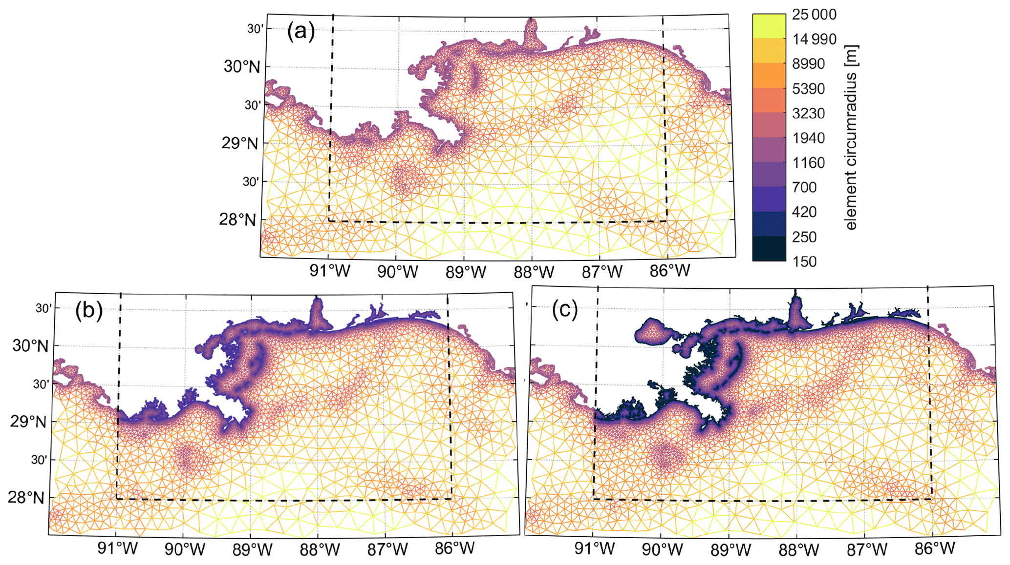
Figure 2Comparisons of mesh triangulation and resolution (defined as the element circumradius on a Lambert conformal conic projection) in the Hurricane Katrina landfall region around Louisiana–Mississippi, USA. (a) MinEle = 1.5 km (default TLS-B global mesh design), (b) MinEle = 500 m local mesh refinement, (c) MinEle = 150 m local mesh refinement. The black dashed boxes indicate where the local mesh refinement was applied.
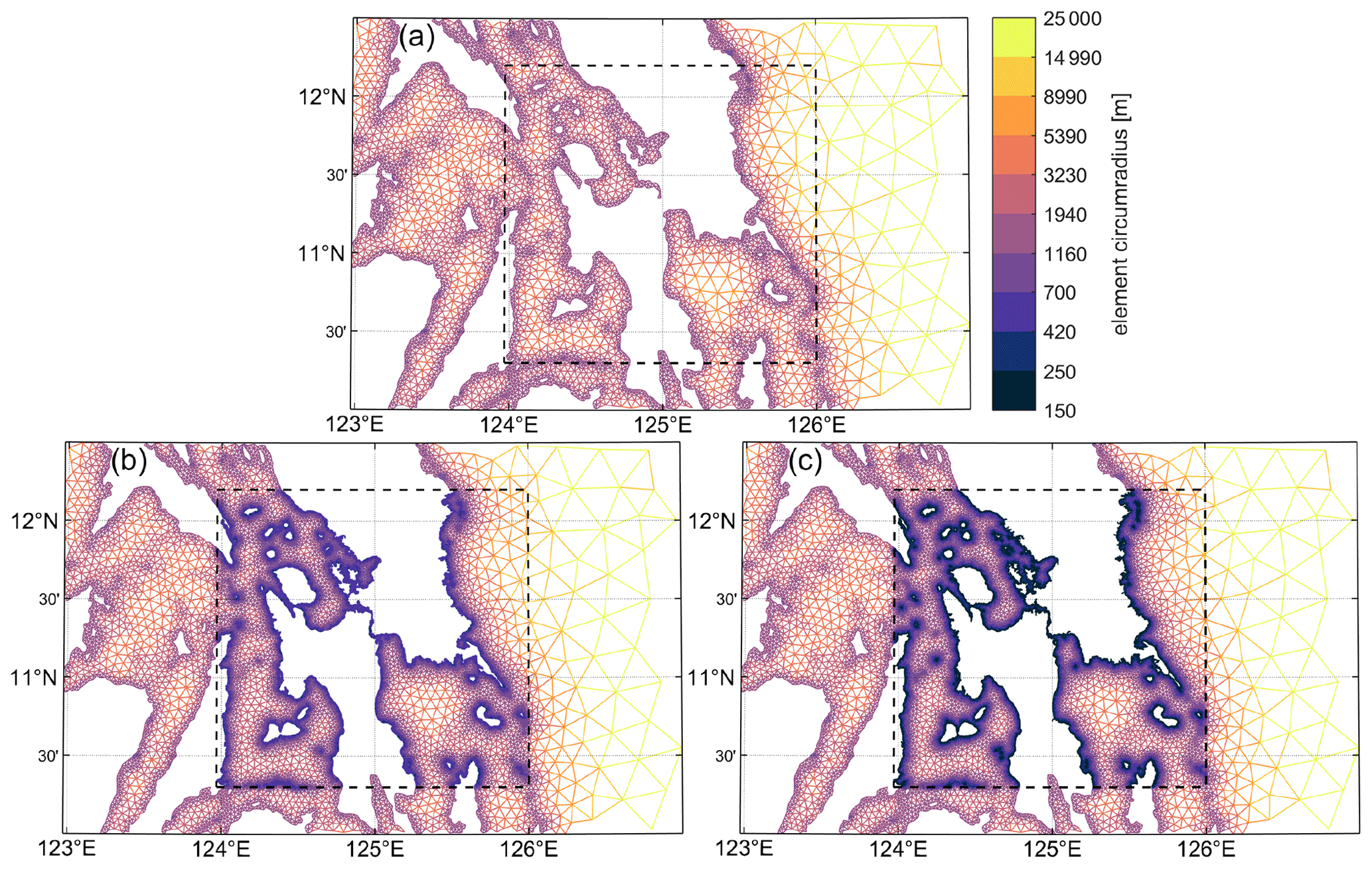
Figure 3Comparisons of mesh triangulation and resolution (defined as the element circumradius on a Lambert conformal conic projection) in the Super Typhoon Haiyan landfall region around Leyte and Samar Island, Philippines. (a) MinEle = 1.5 km (default TLS-B global mesh design), (b) MinEle = 500 m local mesh refinement, (c) MinEle = 150 m local mesh refinement. The black dashed boxes indicate where the local mesh refinement was applied.
To assess the accuracy and intercompare mesh designs, we primarily use the output of the maximum simulated storm tide elevation from each event. For validation we compare to surveys of high-water marks (HWMs) in the landfall regions that are located close to the coast (within 1.5 km of the nearest 150 m locally refined mesh vertex) and attributed primarily to surge for both Katrina (URS Group Inc, 2006a, b) and Haiyan (Mori et al., 2014). Note that for Katrina we add a value of 0.23 m to the simulated storm tide elevations to account for a steric offset and the conversion to NAVD88 vertical datum from local mean sea level (Bunya et al., 2010). No adjustment is made for Haiyan. The standard RMSE, the mean absolute error (MAE), and its standard deviation (SD) are reported. In addition, for Katrina we plot the storm tide time series signal at three coastal NOAA tide gauges with available historical data (IDs: 8735180, 8743281, 8761724). For Haiyan, no reliable time series observations of the main event are available (Mori et al., 2014), so we compare to the astronomical tide reconstructed from TPXO9-Atlas constituents at three selected locations for reference. The geographical location of the HWMs, tide gauges, and selected locations are shown with the results in Sect. 3.2.
2.4 Datasets and model setup
The full-resolution Global Self-consistent Hierarchical High-resolution Shorelines (GSHHS) dataset (Wessel and Smith, 1996) is used to define the shoreline boundary when making the mesh. The most recent global bathymetry DEM, GEBCO_2019 (GEBCO Compilation Group, 2019), which has an equatorial resolution of ∼500 m, is used to prescribe the bathymetry for the model (Sect. S2.2). Underneath Antarctica ice shelves, the RTopo-2 DEM (Schaffer et al., 2016), which has an equatorial resolution of ∼1 km, is used to prescribe ocean depths, taking into account the ice shelf thickness. The SAL tide is specified from the FES2014 (Lyard et al., 2006) data-assimilated tidal solutions (Sect. S2.4). The buoyancy frequency data required to compute the internal wave drag tensor, 𝒞 (Sect. S2.6), are calculated from the 2005–2017 decadal average of salinity and temperature data taken from the World Ocean Atlas 2018 (Locarnini et al., 2019; Zweng et al., 2019). We note here that the accuracy of global tidal solutions strongly depends on the quality of the bathymetric data, the internal wave drag tensor, and the bottom stress term, which can all be tuned to minimize tidal errors (e.g., Pringle et al., 2018a; Lyard et al., 2020). Since this study is focused on the effects of mesh design and the improvements to the governing equations in the new version of the ADCIRC model, we deliberately avoided excessive tuning of the model that aims to minimize tidal solution errors. Instead we chose to use a global constant value of Cit, which gives the same available potential tidal energy compared to the TPXO9-Atlas, and employ a global constant Cf of 0.0025 except in the Indian Ocean and western Pacific Ocean where it spatially varies per the specifications by a previous study of ours (Pringle et al., 2018a) (see Sect. S2 for additional details of model specifications).

Figure 4Maximum 10 m wind velocities and minimum pressure contours over the ocean for Hurricane Katrina (25–31 August 2005) and Super Typhoon Haiyan (4–10 November 2013). (a) Global view displaying CFSR reanalysis data during Katrina except in the Gulf of Mexico region (indicated by the black dashed box labeled GOM); (b) Gulf of Mexico region displaying OWI reanalysis data of Katrina; (c) Philippine Sea region (indicated by the black dashed box labeled PS in panel a) displaying the best-track Holland parametric vortex model of Haiyan. Black dashed boxes in (b) and (c) indicate the landfall regions where the mesh is locally refined for each storm.
Atmospheric forcings are derived from three different sources in this study (see Sect. S2.5 for details on how to use each source in ADCIRC v55). Hourly global reanalysis datasets, 0.313∘ Climate Forecast System Reanalysis (CFSR) (Saha et al., 2010) for Katrina and 0.205∘ CFSv2 (Saha et al., 2014) for Haiyan, are used outside the local storm regions (Fig. 4a). Locally in the Gulf of Mexico region, Hurricane Katrina is forced by 15 min 0.050∘ OceanWeather Inc. (OWI) atmospheric reanalysis data (Bunya et al., 2010) from 25 to 31 August (Fig. 4b). Super Typhoon Haiyan meteorology is described by the best-track Holland parametric vortex model (Holland, 1980) from 4 to 10 November (Fig. 4c).
When only astronomical tides are simulated, we force the model with only astronomical forcing (η) for the five leading astronomical tidal constituents (M2, S2, N2, K1, O1) and analyze for the corresponding constituent amplitude and phases using a 28 d harmonic analysis. These five constituents are chosen so that we can use a relatively short 28 d harmonic analysis period (Ngodock et al., 2016), which would otherwise need to be extended to around 180 d if other constituents were included because of the closeness in their frequencies (e.g., K1 and P1) (Pringle et al., 2018a). When simulating storm tides, both atmospheric (τw and ps) and astronomical forcings are invoked, this time using the following 10 tidal-potential-generating constituents to obtain a more complete tidal signal: M2, S2, N2, K2, O1, P1, K1, Q1, MF, MM. In both cases the model is spun up from a quiescent state for approximately 4 weeks to make sure that global tides are in relative equilibrium. Complete specification details to set up the ADCIRC v55 model simulations in this study are detailed in Sect. S2 in the Supplement.
3.1 Global mesh design
3.1.1 Validation of the reference mesh
When simulating on the Ref mesh using ADCIRC v55, significant improvements to the prediction of astronomical tidal constituents were measured compared to ADCIRC v54. In particular, M2 amphidromes in the high-latitude regions are largely corrected such that any disparities between TPXO9-Atlas and our updated model solutions are qualitatively hard to discern from a global perspective (Fig. 5). Moreover, M2 RMSEt is less than 2.5 cm over most of the ocean, with the largest remaining deep-ocean hotspot in the North Atlantic (Fig. 6). The deep-ocean M2 cm (Table 3) is smaller than for the majority of previously non-assimilated barotropic tidal models (Stammer et al., 2014; Schindelegger et al., 2018) and within the range of errors computed for solutions obtained by embedding a state ensemble Kalman filter (perturbed data assimilation) into a forward ocean circulation model (Ngodock et al., 2016). The recent study by Lyard et al. (2020) carefully tunes local bathymetric data and dissipation parameters (Cf and Cit) to obtain smaller errors (M2 cm) than presented here. As noted in Sect. 2.4, in this study we deliberately avoided excessive tuning of the model with the aim to minimize tidal solution errors. Nevertheless, the five-constituent total tidal error, , is less than 4 cm in the deep ocean. In shallow regions, the M2 is 13.9 cm, which is essentially the same as presented in Schindelegger et al. (2018) but significantly greater than in Lyard et al. (2020). The total tidal error in shallow water, , is 17.2 cm, but note that the area-weighted median value of RMSEt|tot (see Appendix A) in shallow water is just 6.63 cm.
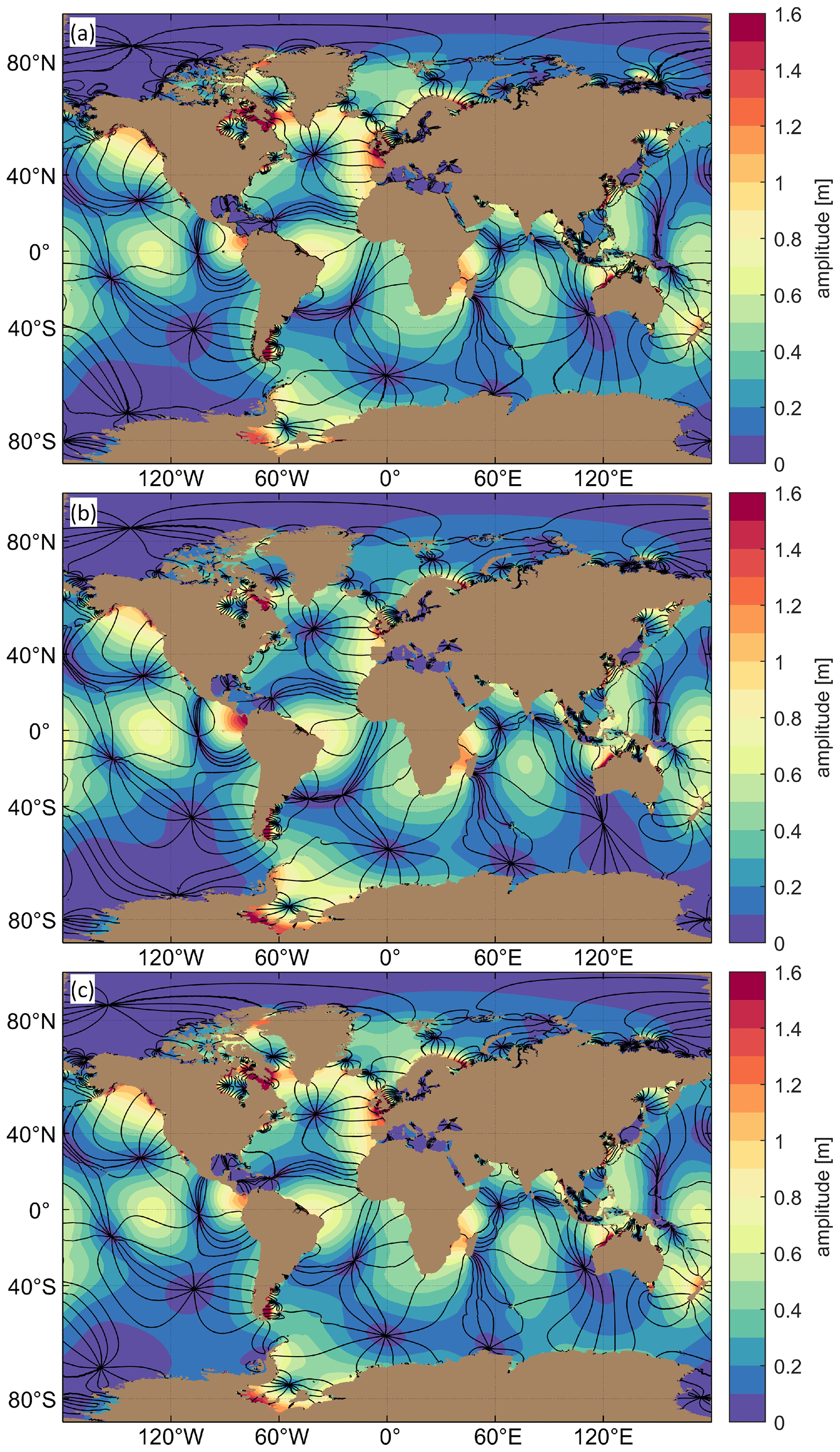
Figure 5Global M2 tidal amplitude and phase (cotidal lines are drawn in 30∘ increments) plots for (a) TPXO9-Atlas, (b) ADCIRC v54 on the Ref mesh, and (c) ADCIRC v55 upgrade on the Ref mesh.

Figure 6Global M2 RMSEt computed against the TPXO9-Atlas for (a) ADCIRC v54 on the Ref mesh, (b) ADCIRC v55 upgrade on the Ref mesh, and (c) ADCIRC v55 upgrade on the TLS-B mesh.
Table 3 (cm; see Appendix A) values for simulated tidal results using ADCIRC v55 (upgrade) and ADCIRC v54 in deep (h>1 km) and shallow (h<1 km) waters on the Ref mesh. Results from other forward barotropic tidal models (Stammer et al., 2014; Ngodock et al., 2016; Schindelegger et al., 2018; Lyard et al., 2020) are included for comparison where known.
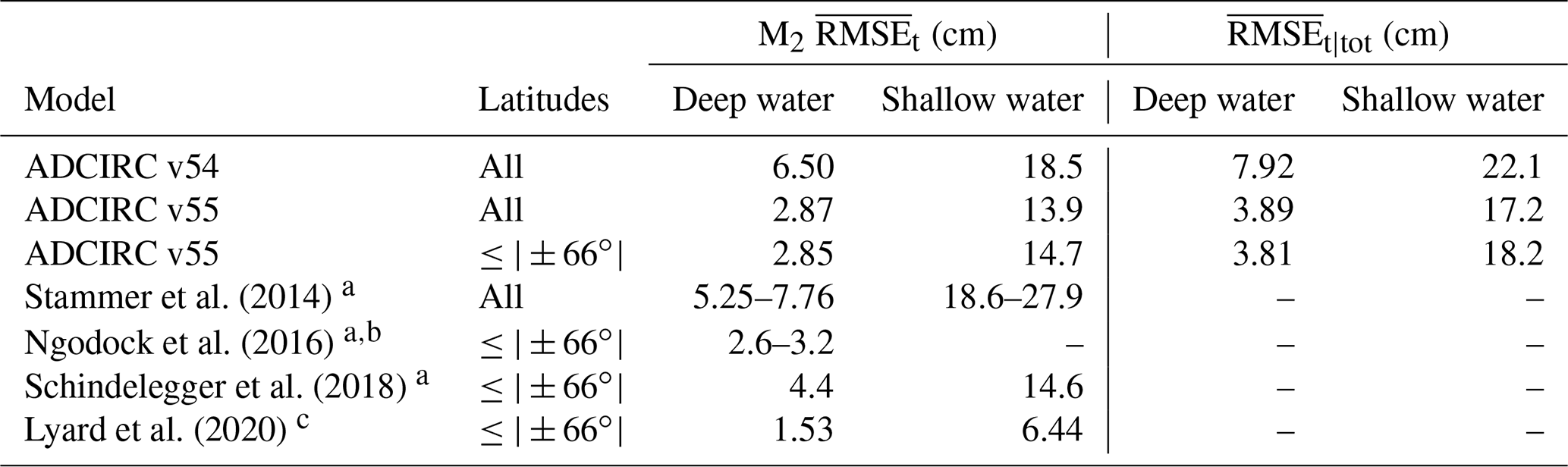
a is computed against TPXO8-Atlas rather than TPXO9-Atlas. b Uses state ensemble Kalman filter (perturbed data assimilation). c results for hydrodynamic FES2014 computed against satellite crossover points.
3.1.2 Solution variability with global mesh design parameters
The distribution (ECDF curves) of RMSEt|tot degrades as the mesh size function parameters are relaxed (Fig. 7). Most of this degradation occurs in the body of the distribution rather than the tails. This characteristic implies that the K test statistic is a good metric of disparity between mesh designs (Fig. 8) because it measures the greatest vertical distance between ECDF curves that has a greater chance of being larger in the body. K is positive for all mesh designs, indicating that the Ref mesh is indeed statistically the best-performing mesh.
Increasing MinEle has a clear but gradual degenerative effect on the solution as it is increased from 1.5 to 3 km. The disparities in the ECDF curves noticeably grow as MinEle is increased to 6 km; the value of K increases from 0.057 for 3 km to 0.175 for 6 km. In comparison, the ECDF curves and the value of K are changed comparatively little as the TLS parameter is decreased from 20 to 5 (K is just 0.032 for TLS = 5). In fact, the solutions are close to identical for TLS values of 10 and 20. However, as the TLS function is turned off (TLS = 0), the solution is severely degraded and the value of K is the greatest for any mesh design (=0.257). The effect of using the FL function and relaxing the parameter on the ECDF curves is fairly gradual overall. However, the magnitude of this change is not trivial; K is increased to 0.070 for FL .
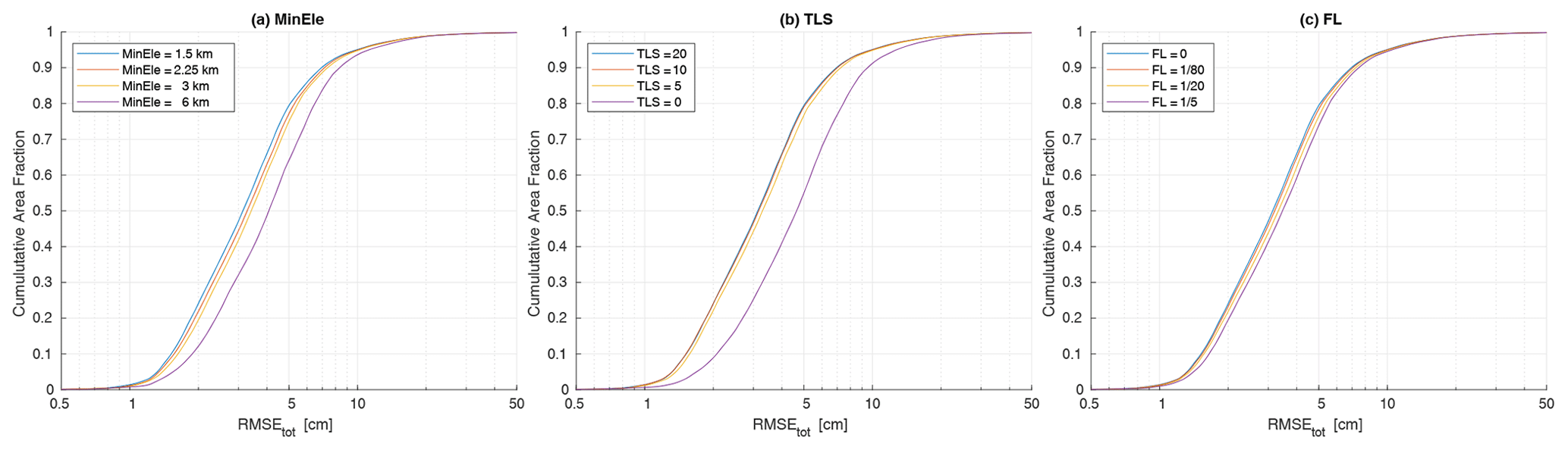
Figure 7Area-weighted ECDF curves of RMSEt|tot for the global mesh designs varying MinEle (a), TLS (b), and FL (c). See Table 2 for mesh design details.
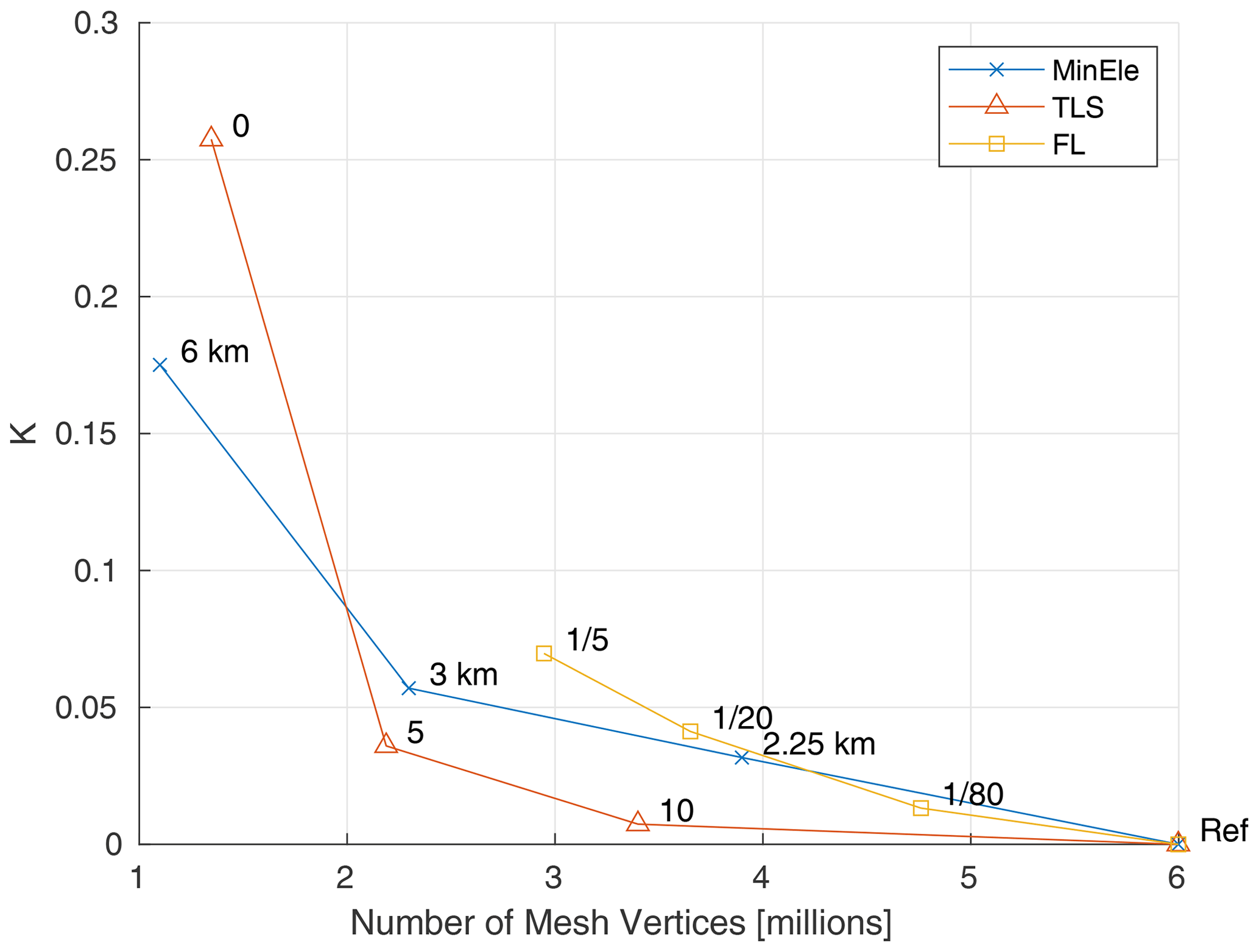
Figure 8The two-sample Kolmogorov–Smirnov test statistic, K, versus the total number of mesh vertices. K is computed as the largest vertical distance between the RMSEt|tot ECDF curve of the Ref mesh design and the ECDF curve of the coarsened mesh designs (varying MinEle, TLS, and FL; Table 2).
In summary, the results demonstrate that decreasing the TLS parameter from 20 to 5 substantially decreases the number of vertices, while it has a relatively small effect on the tidal solution compared to the other experiments. On the other hand, increasing the FL parameter has a comparatively small impact on vertex count reduction, while increasing MinEle has a relatively large impact on the solution. The final choice of mesh design is dependent on one's tolerance for error, but in general it is preferable to choose a mesh that is plotted close to the bottom left corner of the graph in Fig. 8. Following this logic, the TLS-B mesh design (MinEle = 1.5 km, TLS = 5, FL = 0) appears to be the most efficient one tested (see Fig. 6 for the spatial distribution of M2 RMSEt on this mesh). The results also suggest that combinations of MinEle larger than 1.5 km (∼2.25–3 km) and a TLS parameter smaller than 20 (∼5–10) could be employed to potentially lead to an efficient mesh design. Nevertheless, using a small MinEle is in and of itself useful to provide extra coastal resolution, which may be more important as we consider local storm tide accuracy. Thus, TLS-B is chosen as the base mesh design in Sect. 3.2.
3.2 Local mesh refinement
3.2.1 Validation on the 150 m locally refined meshes
The maximum storm tide elevation due to Hurricane Katrina approaches 8 m in the Hancock and Harrison counties of Mississippi (Fig. 9a), comparable to previously obtained high-fidelity simulation results (Dietrich et al., 2009). For Super Typhoon Haiyan, the maximum storm tide elevation exceeds 6 m near Tacloban due to local amplification in the Leyte Gulf (Fig. 9b), similar to previous simulation results (Mori et al., 2014). Qualitatively good agreement with the plotted HWMs is demonstrated for both storms, with a few exceptions.
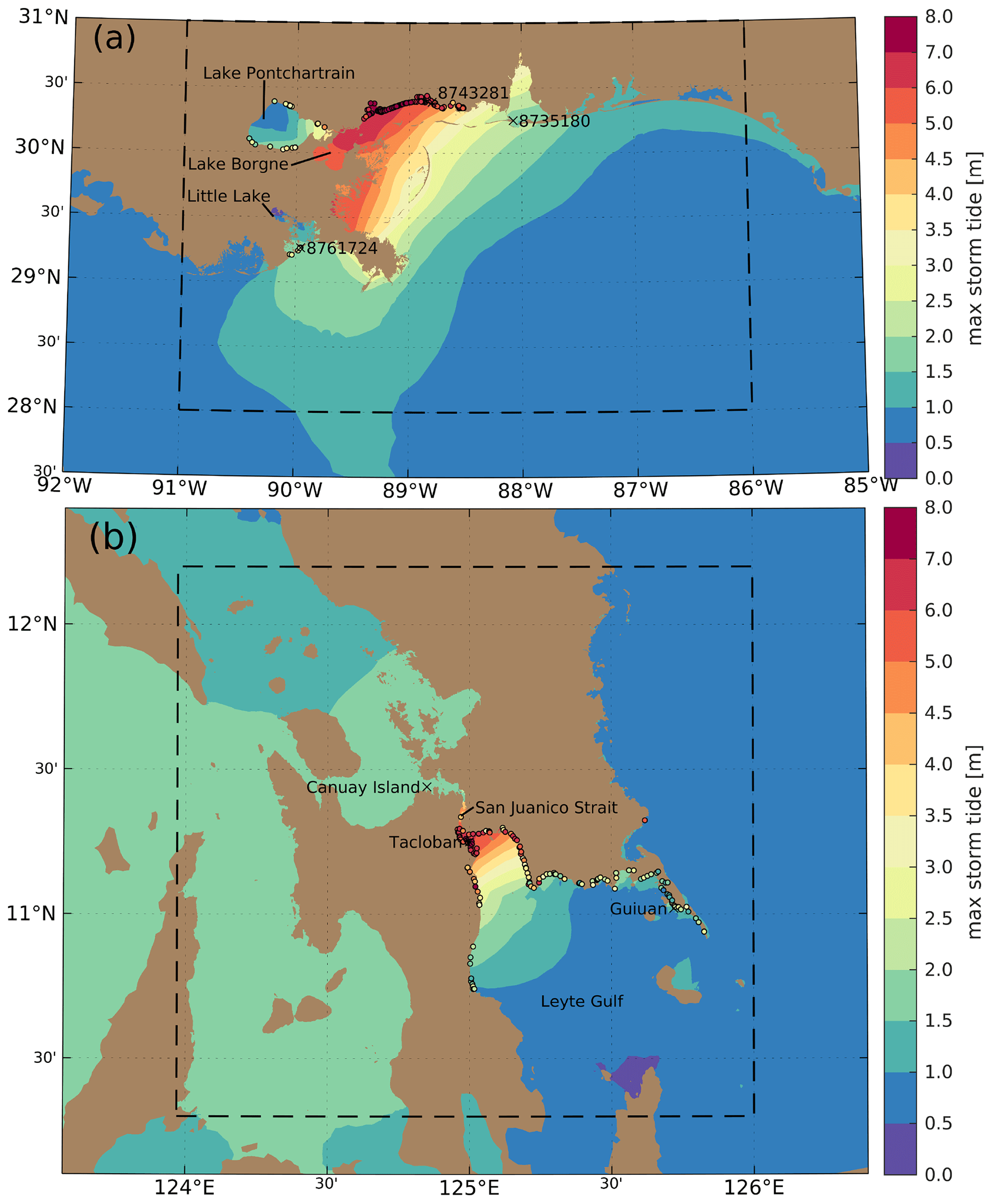
Figure 9Maximum simulated storm tide elevations on the MinEle = 150 m local refinement meshes compared to coastal-surge-attributed high-water marks that are located within 1.5 km of the mesh coastline (filled circles). Black annotated crosses indicate the locations where storm tide time series are plotted. (a) Maximum simulated elevations due to Hurricane Katrina in the Louisiana–Mississippi landfall region. A value of 0.23 m has been added to account for a steric offset and the conversion to NAVD88 vertical datum from local mean sea level. (b) Maximum simulated elevations due to Super Typhoon Haiyan in the Leyte and Samar Island, Philippines, landfall region.
As pointed out by Mori et al. (2014), since inundation is not simulated and the effects of wave setup are ignored in these simulations we expect the maximum storm tide height to match the lower envelope of observed HWMs due to the amplification by topography (although ignoring inundation in our simulations is expected to overestimate the seaward maximum storm tide heights that likely cancels out some of the otherwise low bias when compared to HWMs; Idier et al., 2019). By numbering the HWMs starting at the most southwest point and following the shoreline clockwise, it is indeed illustrated that the simulation results tend to match the lower envelope of observed HWMs quite closely (Fig. 10). For Katrina, the MAE = 1.06 m (SD = 0.66 m) (see Fig. 10 legend for error statistics) from 138 HWMs is larger than the MAE = 0.36 m (SD = 0.44 m) based on 193 HWMs in Bunya et al. (2010). However, their simulations included wave setup, river flows, levees, and dynamic inundation, so our results can be considered quite reasonable in comparison. For Haiyan, the RMSE = 1.45 m from 145 HWMs closely matches the RMSE range of 1.29–1.45 m based on 60 HWMs in Mori et al. (2014). The large scatter present in the HWM measurements (SD ≈1.3 m for all MinEle) could be related to the generation of infragravity waves over fringing reefs in the region, leading to amplified coastal run-up (Roeber and Bricker, 2015).
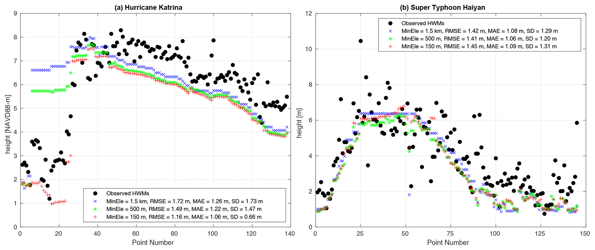
Figure 10Comparisons of the observed HWMs to the simulated maximum storm tide height at the nearest vertex on meshes with different local MinEle (1.5 km, 500 m, 150 m). (a) Hurricane Katrina (0.23 m has been added to simulated results) and (b) Super Typhoon Haiyan. Points are numbered by starting from the most southwest point and following the shoreline clockwise around.
Time series of Hurricane Katrina at NOAA tide gauges show that the timing of the peak storm tide elevation and the amplitude and phase of the tide signal prior to landfall are well-represented by the model (Fig. 11). The modeled peak is underestimated by ∼0.4 m at gauge 8735180, and at gauge 8743281 where the largest peak storm tide occurred, tide gauge recording was interrupted as the storm was making landfall, but the simulation closely follows the observations until this point. A roughly constant discrepancy of ∼0.4–0.5 m between the simulation and observation develops at the gauges following the last high tide prior to storm landfall, likely explaining the underestimate at gauge 8735180 (by this logic the peak may be overestimated at 8761724). We think that this negative bias is mostly attributable to the insufficient generation of the surge forerunner and partly also to the omission of regional wave setup. The surge forerunner is generated through the Ekman setup process (Kennedy et al., 2011), which is crudely represented by the depth-averaged model used here. Previous depth-averaged ADCIRC-based studies using a Manning's bottom friction formulation so that Cf becomes very small on the continental shelf appear to be better able to generate the surge forerunner, as well as employing wind–wave coupling to generate wave setup, indeed show better agreement with the time series prior to the peak storm tide (Bunya et al., 2010; Roberts and Cobell, 2017). Time series of Super Typhoon Haiyan also show that the amplitude and phasing of the tide at the selected locations are fairly well-represented compared to the TPXO9-Atlas (Fig. 11). Storm tide heights at Tacloban are dominated by the short and intense surge event, but the duration of surge is likely underestimated because the parametric vortex model lacks background winds. Due to the timing of the storm landfall during the lower high tide, peak storm tides exceeded the higher high tide by just 0.5 m at Guiuan. In fact, for Guiuan and Canuay Island the minimum storm tide levels were more severe than the peak levels.
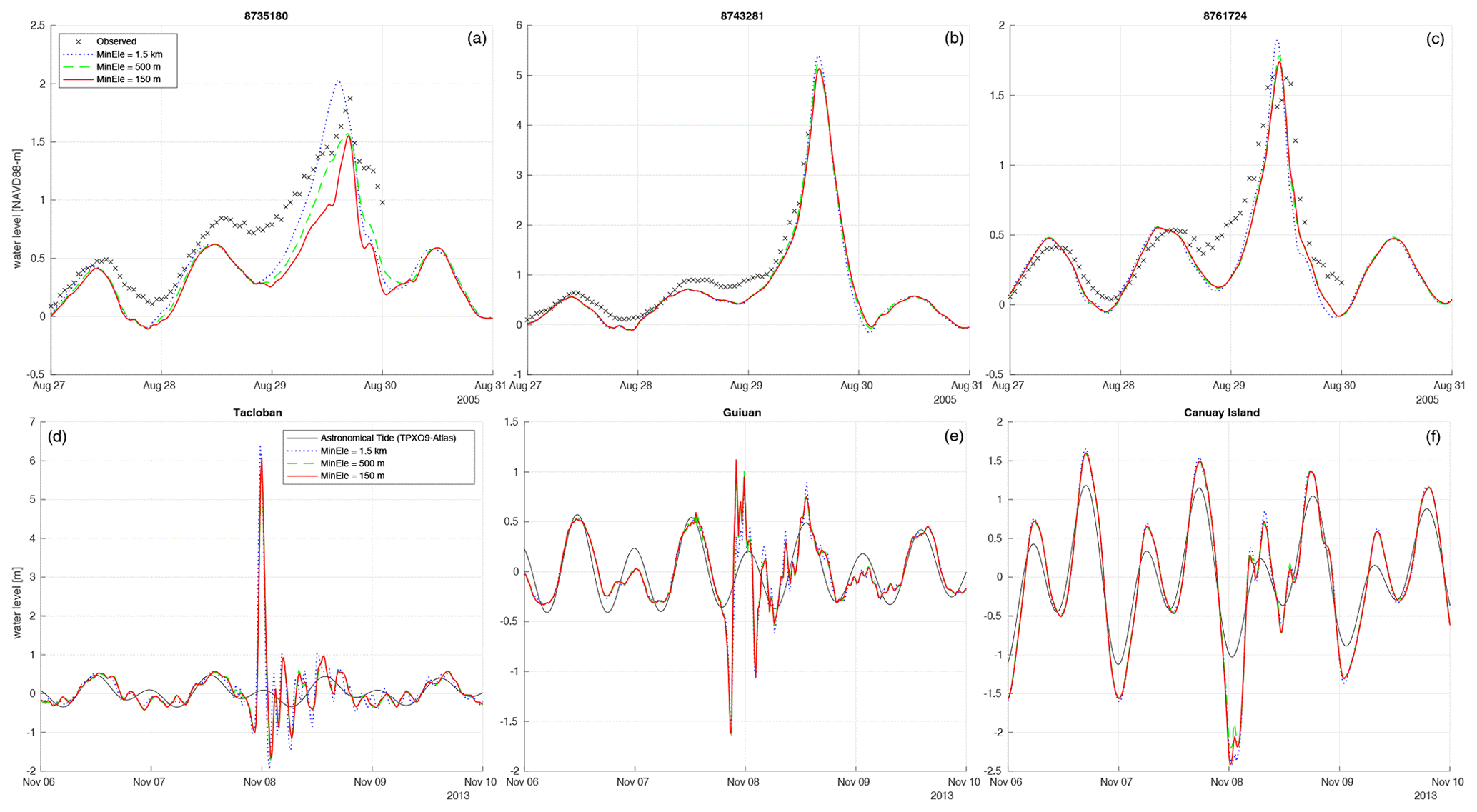
Figure 11Comparisons of simulated storm tide elevation time series on meshes with different local MinEle (1.5 km, 500 m, 150 m) at the point locations shown in Fig 9. (a–c) Hurricane Katrina compared to NOAA tide gauge observations (0.23 m has been added to simulated results). (d–f) Super Typhoon Haiyan compared to the astronomical tide reconstructed from the TPXO9-Atlas.
3.2.2 Solution variability with local mesh refinement
Our results indicate that there is a tendency for the coarser-resolution meshes to have larger storm tide elevations in the open coastal areas of the landfall region. In the case of Katrina, this is most clearly seen in Lake Borgne where maximum storm tide elevations are at least 0.6 m larger on the MinEle = 1.5 km mesh than those on the MinEle = 500 m mesh and approximately 0.2 m larger on the MinEle = 500 m mesh than the MinEle = 150 m mesh (Fig. 12). Interestingly, neither the MinEle = 1.5 km mesh nor the MinEle = 500 m mesh includes Lake Pontchartrain, while the MinEle = 150 mesh does (Fig. 2). This is because the Rigolets Strait connecting Lake Pontchartrain to Lake Borgne is approximately 500 m at its narrowest, and thus the MinEle = 500 m mesh is at the cutoff point for meshing the strait and providing hydraulic connectivity between the two lakes. Yet, the maximum elevation difference from Lake Borgne across to Mobile Bay between MinEle = 1.5 km and MinEle = 500 m is still much greater than between MinEle = 500 m and MinEle = 150 m (refer to the time series at gauges 8735180 and 8743281 in Fig. 11 and Fig. 12). Nevertheless, since MinEle = 150 m is the only mesh to resolve Lake Pontchartrain, the HWMs surrounding the lake (point numbers 7–23) can only be reasonably estimated by simulations on this mesh, resulting in the smallest HWM error statistics (Fig. 10a).
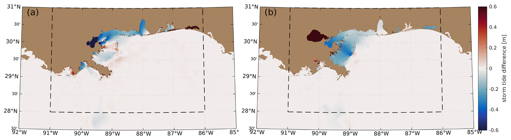
Figure 12Mesh-resolution-induced differences in the simulated maximum storm tide elevations due to Hurricane Katrina in the Louisiana–Mississippi landfall region. (a) Elevations on the MinEle = 500 m local refinement mesh minus elevations on the TLS-B global mesh (MinEle = 1.5 km). (b) Elevations on the MinEle = 150 m local refinement mesh minus elevations on the MinEle = 500 m local refinement mesh. In areas where the coarser-resolution mesh does not exist the value shown is just the maximum storm tide elevation on the higher-resolution mesh.
In the case of the Haiyan, the predominant maximum storm tide elevation difference (∼0.4–0.6 m) is located at the back of Leyte Gulf near Tacloban between the MinEle = 1.5 km and MinEle = 500 m meshes (Figs. 11 and 13). The decrease in elevations in the MinEle = 1.5 km mesh might be explained by the omission of the San Juanico Strait (∼800 m wide at its narrowest; Fig. 3). In contrast, the elevations near Tacloban and in the strait increase by up to 0.6 m as the MinEle = 500 m mesh is refined to MinEle = 150 m. There is also a reduction in the elevations (by up to 0.2 m) just offshore of the Leyte Gulf along the shelf break for the coarser meshes, which is better represented in the higher-resolution renditions. Overall, the choice of local MinEle has a small effect on the representation of HWMs for Haiyan (Fig. 10b). The only major noticeable impact is for the HWMs near Tacloban in the San Juanico Strait (point numbers 25–63) on the MinEle = 1.5 km mesh. Since this mesh does not resolve the strait, the simulated estimates of the HWMs here are all taken from the same or nearby mesh vertices at the back of the gulf.
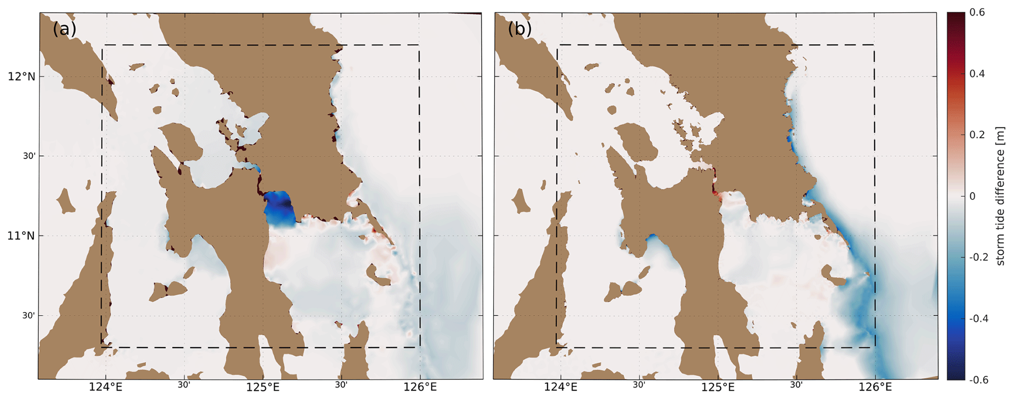
Figure 13Mesh-resolution-induced differences in the simulated maximum storm tide elevations due to Super Typhoon Haiyan in the Leyte and Samar Island, Philippines, landfall region. (a) Elevations on the MinEle = 500 m local refinement mesh minus elevations on the TLS-B global mesh (MinEle = 1.5 km). (b) Elevations on the MinEle = 150 m local refinement mesh minus elevations on the MinEle = 500 m local refinement mesh. In areas where the coarser-resolution mesh does not exist the value shown is just the maximum storm tide elevation on the higher-resolution mesh.
Lastly, we mention two additional general observations. First, for both storms the far-field effects of local mesh refinement were found to be negligible. Second, storm tide elevation time series show that not only does the peak elevation tend to decrease as mesh refinement is made, but the timing of the peak also tends to occur later (Fig. 11), as is most clearly illustrated for gauge 8735180.
3.3 Computational performance
For all astronomical tide simulations performed in the global mesh design experiments (Sect. 3.1) the time step, Δt, was set to 120 s, which is equivalent to a Courant (CFL) number of 5–22 on the global mesh designs used in this study (see Sect. S1.5 for model stability details). The resulting computational wall-clock times for the astronomical tide simulations ranged from 5 to 30 s per simulation day depending on the total vertex count of the mesh (Fig. 14). All simulations were computed on 480 Haswell processors with a Mellanox FDR Infiniband network connection.
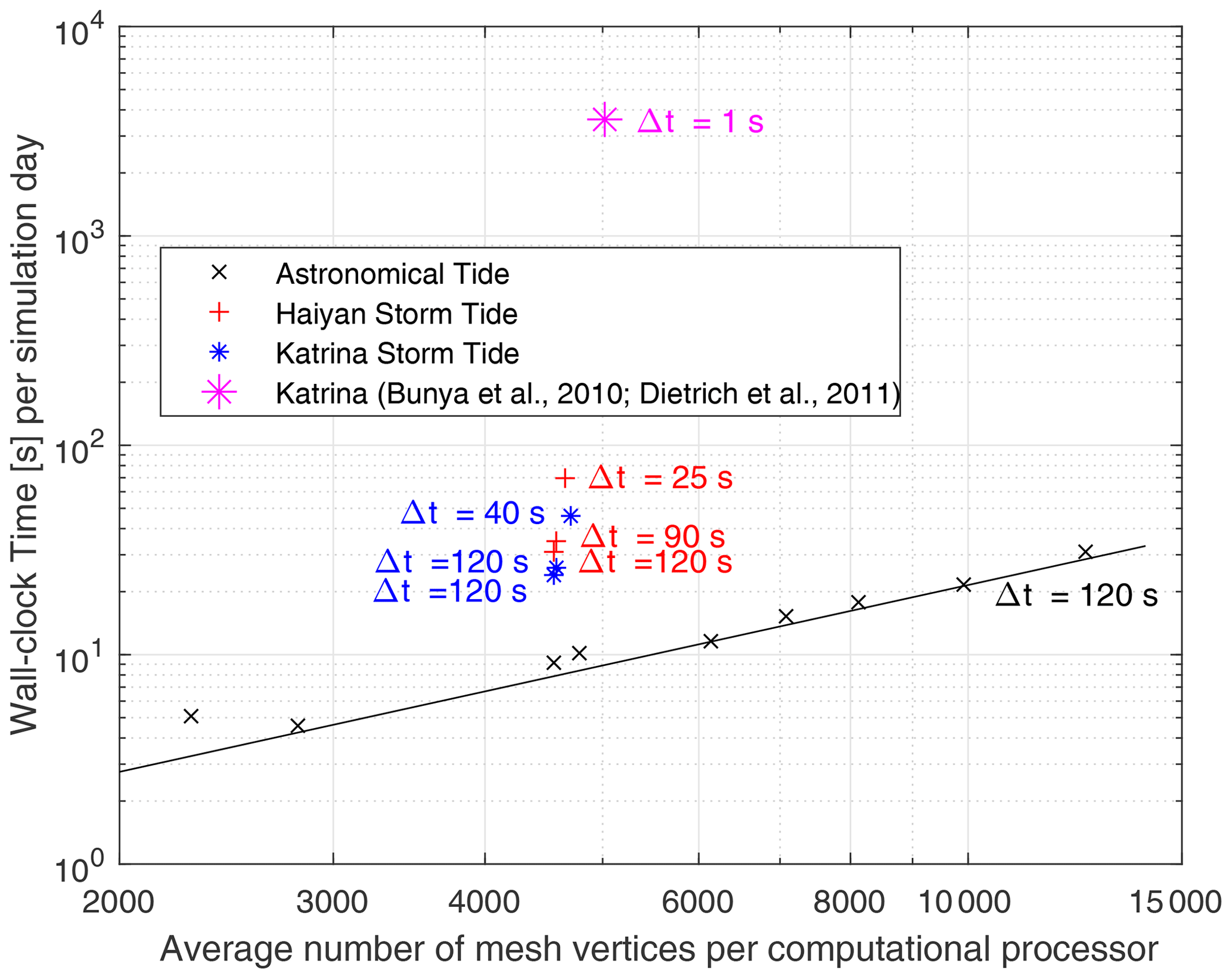
Figure 14Computational wall-clock times for the various mesh designs and experiments versus the average number of mesh vertices per computational processor. All simulations were computed on 480 computational processors (i.e., the variation in vertices per processor comes from the variation in the total number of vertices for each mesh design). The computational performance in this study using ADCIRC v55 is contrasted with previous ADCIRC model Katrina storm tide simulations (Bunya et al., 2010; Dietrich et al., 2011) that required very small time steps (Δt=1 s).
For the storm tide simulations performed in the local mesh refinement experiments (Sect. 3.2) the time step had to be reduced for finer meshes due to model instability related to nonlinear terms that are treated explicitly, which become more significant as element sizes near the shore (in shallow depths) are reduced. For Katrina, the time step for the MinEle = 150 m mesh had to be reduced to 40 s. For Haiyan, the time step had to be reduced for both the MinEle = 500 m (Δt=90 s) and the MinEle = 150 m (Δt=25 s) mesh. The resulting computational wall-clock times were increased for the smaller time steps (Fig. 14). However, the simulations on the MinEle = 150 m meshes were proportionally around 2 times faster per Δt compared to the coarser meshes. This is attributed to the heavy I/O related to reading meteorological data during the simulation that limits computational speed-up as time steps are increased beyond a certain value. In fact, for the same Δt, wall-clock times for the storm tide simulations were 2–3 times longer than the astronomical tide runs, which require I/O only at the very beginning and end of the simulation. Furthermore, the Haiyan simulations were slightly slower than Katrina simulations because of the higher resolution of the reanalysis meteorology (see Sect. 2.4).
In addition, the computational performance of our Katrina simulations is compared to previous ADCIRC model runs (Bunya et al., 2010; Dietrich et al., 2011) that employed Δt=1 s, leading to wall-clock times 1 to 2 orders of magnitude greater than those in this study (Fig. 14). We remark that the Bunya et al. (2010) and Dietrich et al. (2011) studies used finer mesh sizes (MinEle = 50 m) and included the floodplain, leading to more wetting–drying, which can be a source of numerical instability. Our results nonetheless indicate the potential for substantial computational speed-up on suitably designed meshes.
The new version of ADCIRC (v55) demonstrated improved tidal solutions compared to the previous versions of ADCIRC (denoted as ADCIRC v54). This is because ADCIRC v54 does not solve the correct form of the governing equations in spherical coordinates and is thus technically valid only for sufficiently small regional domains (see Sect. S1.2 for more details on this comparison). For instance, this old form of the governing equations appears to be sufficient for the western North Atlantic Ocean regional domain, which has been thoroughly validated using ADCIRC since Westerink et al. (1994). The changes made in ADCIRC v55 make it suitable for simulating larger domains, in particular the global domains that we investigated in this study.
Results from the global mesh design experiments echo those found previously for a regional mesh of the western North Atlantic Ocean (Roberts et al., 2019b). Namely, when employing a relatively large element-to-element gradation limit (G) of 35 % used here, the TLS function is critical to ensure that water elevation solutions remain accurate by adequately resolving topographic features of importance. The relatively high value of G ensures that the mesh size rapidly enlarges in areas where no topographic gradient features exist to help avoid excessive mesh vertex counts. An interesting point of difference that we note in this study is the interplay between MinEle and TLS. MinEle not only controls the minimum coastal resolution, but it also controls the minimum resolution that can be applied along topographic gradient features in the TLS function. Here, the MinEle ranged between 1.5 and 6 km, which affected the strength of the TLS function in these mesh designs. Nevertheless, the MinEle-C design (MinEle = 6 km) was still superior to the TLS-C one (TLS = 0). There may be additional sensitivity to the TLS function at MinEle less than 1.5 km, although it is likely quite small. In Roberts et al. (2019b), MinEle = 1 km was used along the outer shelf and shelf break, and this appeared to be sufficient.
The results also show that the use of the barotropic Rossby-radius-based low-pass filter (FL) in the TLS function is able to reduce mesh vertices without substantially degrading the solution. However, our results suggest that it is more efficient to simply reduce the TLS value to 5 compared to using TLS = 20 with FL. Combinations of TLS values between 5 and 10 with FL (–) could also be applied depending on the tolerance to the solution accuracy. Using the FL parameter in more highly resolved local domains may also provide benefits to avoid over-resolving topographic slopes in shallow depths. However, it must also be recognized that length scales of importance transition from Rossby radius scaling in the open ocean to those of shoreline features near the shore (LeBlond, 1991). Therefore, a more intelligent low-pass filter may be necessary for such applications.
The astronomical tide solution differences between global mesh designs were shown to be predominantly in the body of the area-weighted ECDF curves, while the tails were almost identical. This implies that simulated tides over most of the area of the ocean are affected by mesh resolution. However, in regions where the tidal range and error are large, which inevitably occurs on shallow shelves, all of the mesh designs have similarly large errors. This perhaps explains why a ∘ tidal model (Schindelegger et al., 2018) could obtain a similar M2 in shallow waters as our more highly resolved reference mesh (14.6 cm compared to 13.9 cm). There is likely an inherent uncertainty in the bathymetry and dissipation that prevents a further decrease in the shallow-water , which can be dominated by large errors (in shallow water the area-weighted median RMSEt|tot is much smaller than ). Indeed, a recent study conducts a 432-member ensemble of perturbations to bathymetric depths, as well as bottom friction and internal wave drag coefficients to obtain smaller tidal errors than this study, particularly in shallow water (Lyard et al., 2020).
The local mesh refinement technique was demonstrated to be a useful tool to provide high refinement with a trivial addition to the total vertex count. Nevertheless, we found that the numerically stable time step decreases as coastal mesh resolution becomes finer (see Sect. S2.1 for details on setting the time step), which increases computational time. Note that additional tests (not shown) were conducted, and these demonstrated that the computational time step used for the same mesh had a negligible effect on storm tide elevation solutions. However, this may not transfer as well for simulations in which there is significant wetting–drying due to the one element per time step wetting–drying logic used. The impact of mesh refinement clearly tends to decrease open-ocean storm tide elevations in open-ocean areas, and the timing of the peak occurs later. This could be attributed to larger physical approximation errors of the shoreline geometry and bathymetry with mesh coarsening (see Roberts et al., 2019b), leading to slightly different wave speeds and wave transformation. In practice, higher peak storm tide heights in coarser models translate to greater coastal flooding potential. Including inundation in the model would decrease the storm tide elevations along the coast (Idier et al., 2019), perhaps leading to more similar coastal storm tide elevations between the different mesh resolutions since more flooding may occur in the coarser model. Overall, the impacts of mesh resolution on the HWM errors were relatively small, especially for Super Typhoon Haiyan. However, the presence of more inland lakes and semi-enclosed bays separated by narrow inlets in the Louisiana region meant that simulated Hurricane Katrina HWM estimates in these features were poor unless the MinEle was sufficient to resolve these narrow passages and provide hydraulic connectivity. A recent study using the GTSM global model with ∼5 km coastal refinement (MinEle = 5 km) was used to characterize the spatiotemporal variability of storm-driven surges along western North Atlantic coasts, including surge due to Hurricane Katrina (Muis et al., 2019). Our results would suggest that coarser-resolution meshes are able to reproduce the broader features of surge along open coastal areas quite well. However, such a model cannot be used to predict storm tide levels within the semi-enclosed bays and lakes in the Louisiana region. Furthermore, MinEle = 5 km is above the limit at which global astronomical tide solutions appear to diverge noticeably from MinEle = 1.5 km meshes.
Last, it is widely recognized that sensitivities to local high-resolution bathymetry datasets, internal tide wave drag, and spatially varying bottom friction and surface ice friction are important (Lefevre et al., 2000; Le Bars et al., 2010; Zaron, 2017; Pringle et al., 2018a; Zaron, 2019; Lyard et al., 2020), likely more so than the mesh resolution effects that we concentrate on here. We aim to develop a unified framework for globally calibrating spatially varying internal tide wave drag and bottom friction coefficients with improved local high-resolution bathymetric datasets in future work. Doing so should result in smaller storm tide elevation discrepancies, especially in shallow water (e.g., Lyard et al., 2020). Moreover, we did not simulate inundation in this study, but it will be a crucial future step so that we can forecast and assess coastal flood risks for all of Earth's coasts.
Important upgrades to the FEM SWE solver, ADCIRC, have been presented to improve accuracy and efficiency for global storm tide modeling across multi-resolution unstructured meshes. We systemically tested the new model's (ADCIRC v55) sensitivity to mesh design in the simulation of global astronomical tides and storm tides. These mesh design results are expected to be broadly applicable to other SWE solvers that correctly handle solutions on the sphere.
Based on the results for global mesh design we recommend aiming for a minimum element size less than 3 km and using the TLS function to resolve topographic gradient features with a TLS value of 5–10. Paired with the OceanMesh2D software, the ability to seamlessly apply local refinement allows the user to provide fine coastal resolution in the region of interest (e.g., the storm landfall region) without large increases in the total mesh vertex count (increase of 0.5 %–3 % in this study). We found that in general, peak storm tide elevations along the open coast are decreased (therefore, the coastal flooding potential is decreased) and the timing of the peak occurs later with local coastal mesh refinement. When validated against observed high-water marks measured near the coast, coastal mesh refinement only has a significant positive impact on errors in narrow straits and inlets, as well as in bays and lakes separated from the ocean by these passages.
The new ADCIRC v55 code capable of accurate global storm tide modeling with fine coastal resolution is computationally efficient. For global meshes with nominal minimum resolution as fine as 1.5 km, the computational wall-clock time ranged from 5 to 30 s per simulation day on 480 computational processors for astronomical tide simulations. Some improvements that we made to the numerical stability of the algorithm facilitated the application of relatively large 120 s time steps to achieve this efficiency. However, we found that the locally refined meshes (nominal minimum resolution of 500 and 150 m) often required smaller time steps (25–90 s). Nevertheless, these are still much larger than time steps used in previous studies with older versions of ADCIRC, resulting in computational times 1 to 2 orders of magnitude shorter.
The RMSEt for a single constituent at a point is defined as (Wang et al., 2012)
where A is the tidal amplitude, θ is the tidal phase lag, and the subscripts “o” and “m” refer to the observed (in this case TPXO9-Atlas) and modeled values, respectively. To get the RMSEt of the total five-constituent signal, RMSEt|tot, we use the approximation (Wang et al., 2012)
where k indicates the arbitrary constituent number from the five leading tidal constituents (M2, S2, N2, K1, O1).
The area-weighted ECDF curves of RMSEt|tot are computed through MATLAB's “ecdf” function with the “frequency” input set equal to the elemental area (m2). With this construction, the area-weighted median value of RMSEt|tot is defined as the point of intersection of the ECDF curve with 50 % probability. Comparisons between ECDF curves can be made by taking the largest vertical distance between them to obtain K. We compute K one-sided in that it will be positive if the base (Ref) design is statistically superior and negative otherwise.
To obtain a single number to compare the solutions globally or in certain depths or regions, it is common to use the area-weighted root mean square error of the RMSEt (Arbic et al., 2004),
where ∬dA indicates an area integral. can be computed for a single constituent or for the five-constituent total signal ().
The official release version of ADCIRC is available from the project website at http://adcirc.org/ (last access: 23 February 2021) under the terms stipulated there and is free for research or educational purposes. The exact version of the model used to produce the results used in this paper is archived on Zenodo at https://doi.org/10.5281/zenodo.3911282 (Pringle, 2020), along with the simulated tidal harmonic constituents on the various mesh designs and the simulated storm tide results with the corresponding model setup (Pringle, 2020).
The current version of OceanMesh2D is available from the project website at https://github.com/CHLNDDEV/OceanMesh2D (last access: 23 February 2021) under the GPL-3.0 license. The exact version of the model (V3.0.0) used to generate the meshes in this study is archived on Zenodo at https://doi.org/10.5281/zenodo.3721137 (Pringle and Roberts, 2020).
An application of the presented ADCIRC v55 model (on the TLS-B mesh design) providing 5 d forecasts of global storm surge is currently running in real time, and maximum surge elevations are available to view at https://wpringle.github.io/GLOCOFFS/ (last access: 23 February 2021). The forecast is automatically updated every 6 h based on GFS weather forecast schedules. The simulation wall-clock time is approximately 10 min on 72 computational processors. Images are automatically archived by GitHub.
The supplement related to this article is available online at: https://doi.org/10.5194/gmd-14-1125-2021-supplement.
WJP prepared the paper, designed and implemented the coding upgrades into ADCIRC v55, designed and performed the experiments, and conducted the stability analysis. DW mathematically formulated and initially implemented most of the ADCIRC coding upgrades. KJR and WJP equally contributed to the coding and development of the OceanMesh2D software integral to this study, and KJR provided critical feedback to improve the paper design. JJW provided the research and computing resources as well as the funding necessary to conduct this study.
The authors declare that they have no conflict of interest.
This work was supported by the US Alaska/Integrated Ocean Observing System (AOOS/IOOS) sub-award for US National Oceanic and Atmospheric Administration (NOAA) grant no. NA16NOS0120027, IOOS Ocean Technology Transition Project NOAA grant no. NA18NOS0120164, and NOAA Office of Weather and Air Quality, Joint Technology Transfer Initiative NOAA grant no. NA18OAR4590377.
This research has been supported by the National Oceanic and Atmospheric Administration (grant nos. NA16NOS0120027, NA18NOS0120164, and NA18OAR4590377).
This paper was edited by Claire Levy and reviewed by two anonymous referees.
Arbic, B. K., Garner, S. T., Hallberg, R. W., and Simmons, H. L.: The accuracy of surface elevations in forward global barotropic and baroclinic tide models, Deep-Sea Res. Pt. II, 51, 3069–3101, https://doi.org/10.1016/j.dsr2.2004.09.014, 2004. a
Bouwer, L. M.: Next-generation coastal risk models, Nat. Clim. Change, 8, 7–8, https://doi.org/10.1038/s41558-018-0262-2, 2018. a
Bunya, S., Dietrich, J. C., Westerink, J. J., Ebersole, B. A., Smith, J. M., Atkinson, J. H., Jensen, R., Resio, D. T., Luettich, R. A., Dawson, C., Cardone, V. J., Cox, A. T., Powell, M. D., Westerink, H. J., and Roberts, H. J.: A High-Resolution Coupled Riverine Flow, Tide, Wind, Wind Wave, and Storm Surge Model for Southern Louisiana and Mississippi. Part I: Model Development and Validation, Mon. Weather Rev., 138, 345–377, https://doi.org/10.1175/2009MWR2906.1, 2010. a, b, c, d, e, f, g, h
Castro, M. J., Ortega, S., and Parés, C.: Reprint of: Well-balanced methods for the shallow water equations in spherical coordinates, Comput. Fluids, 169, 129–140, https://doi.org/10.1016/j.compfluid.2018.03.052, 2018. a
Chen, C., Liu, H., and Beardsley, R. C.: An unstructured grid, finite-volume, three-dimensional, primitive equations ocean model: Application to coastal ocean and estuaries, J. Atmos. Ocean. Tech., 20, 159–186, https://doi.org/10.1175/1520-0426(2003)020<0159:AUGFVT>2.0.CO;2, 2003. a
Danilov, S.: Ocean modeling on unstructured meshes, Ocean Model., 69, 195–210, https://doi.org/10.1016/j.ocemod.2013.05.005, 2013. a, b
Dietrich, J., Zijlema, M., Westerink, J., Holthuijsen, L., Dawson, C., Luettich, R., Jensen, R., Smith, J., Stelling, G., and Stone, G.: Modeling hurricane waves and storm surge using integrally-coupled, scalable computations, Coast. Eng., 58, 45–65, https://doi.org/10.1016/j.coastaleng.2010.08.001, 2011. a, b, c
Dietrich, J. C., Bunya, S., Westerink, J. J., Ebersole, B. A., Smith, J. M., Atkinson, J. H., Jensen, R., Resio, D. T., Luettich, R. A., Dawson, C., Cardone, V. J., Cox, A. T., Powell, M. D., Westerink, H. J., and Roberts, H. J.: A High-Resolution Coupled Riverine Flow, Tide, Wind, Wind Wave, and Storm Surge Model for Southern Louisiana and Mississippi. Part II: Synoptic Description and Analysis of Hurricanes Katrina and Rita, Mon. Weather Rev., 138, 378–404, https://doi.org/10.1175/2009mwr2907.1, 2009. a
Dresback, K. M., Kolar, R. L., and Luettich, R. A.: On the Form of the Momentum Equation and Lateral Stress Closure Law in Shallow Water Modeling, in: Estuarine and Coastal Modeling, American Society of Civil Engineers, Reston, VA, 399–418, https://doi.org/10.1061/40876(209)23, 2005. a
Dullaart, J. C., Muis, S., Bloemendaal, N., and Aerts, J. C.: Advancing global storm surge modelling using the new ERA5 climate reanalysis, Clim. Dynam., 54, 1007–1021, https://doi.org/10.1007/s00382-019-05044-0, 2019. a, b
Egbert, G. D. and Erofeeva, S. Y.: Efficient Inverse Modeling of Barotropic Ocean Tides, J. Atmos. Ocean. Tech., 19, 183–204, https://doi.org/10.1175/1520-0426(2002)019<0183:EIMOBO>2.0.CO;2, 2002. a
Egbert, G. D. and Erofeeva, S. Y.: TPXO9-Atlas, available at: https://www.tpxo.net/global/tpxo9-atlas (last access: 23 February 2021), 2019. a
Fortunato, A. B., Freire, P., Bertin, X., Rodrigues, M., Ferreira, J., and Liberato, M. L.: A numerical study of the February 15, 1941 storm in the Tagus estuary, Cont. Shelf Res., 144, 50–64, https://doi.org/10.1016/j.csr.2017.06.023, 2017. a
Fringer, O. B., Dawson, C. N., He, R., Ralston, D. K., and Zhang, Y. J.: The future of coastal and estuarine modeling: Findings from a workshop, Ocean Model., 143, 101458, https://doi.org/10.1016/j.ocemod.2019.101458, 2019. a, b
Funakoshi, Y., Feyen, J. C., Aikman, F., Tolman, H. L., van der Westhuysen, A. J., Chawla, A., Rivin, I., and Taylor, A.: Development of Extratropical Surge and Tide Operational Forecast System (ESTOFS), in: 12th International Conference on Estuarine and Coastal Modeling, 201–212, 7–9 November 2011, St. Augustine, Florida, 2011. a
Garratt, J. R.: Review of drag coefficients over oceans and continents, Mon. Weather Rev., 105, 915–929, 1977. a
Garrett, C. and Kunze, E.: Internal Tide Generation in the Deep Ocean, Annu. Rev. Fluid Mech., 39, 57–87, https://doi.org/10.1146/annurev.fluid.39.050905.110227, 2007. a
GEBCO Compilation Group: GEBCO 2019 Grid, National Oceanography Centre, https://doi.org/10.5285/836f016a-33be-6ddc-e053-6c86abc0788e, 2019. a
Gorman, G. J., Piggott, M. D., Pain, C. C., de Oliveira, C. R., Umpleby, A. P., and Goddard, A. J.: Optimisation based bathymetry approximation through constrained unstructured mesh adaptivity, Ocean Model., 12, 436–452, https://doi.org/10.1016/j.ocemod.2005.09.004, 2006. a
Greenberg, D. A., Dupont, F., Lyard, F. H., Lynch, D. R., and Werner, F. E.: Resolution issues in numerical models of oceanic and coastal circulation, Cont. Shelf Res., 27, 1317–1343, https://doi.org/10.1016/j.csr.2007.01.023, 2007. a
Hervouet, J.-M.: Equations of free surface hydrodynamics, in: Hydrodynamics of Free Surface Flows: Modelling with the Finite Element Method, chap. 2, John Wiley & Sons, Ltd, 5 April 2007, 5–75, https://doi.org/10.1002/9780470319628.ch2, 2007. a
Herzfeld, M., Engwirda, D., and Rizwi, F.: A coastal unstructured model using Voronoi meshes and C-grid staggering, Ocean Model., 148, 101599, https://doi.org/10.1016/j.ocemod.2020.101599, 2020. a
Hoch, K. E., Petersen, M. R., Brus, S. R., Engwirda, D., Roberts, A. F., Rosa, K. L., and Wolfram, P. J.: MPAS-Ocean Simulation Quality for Variable-Resolution North American Coastal Meshes, J. Adv. Model. Earth Syst., 12, e2019MS001848, https://doi.org/10.1029/2019MS001848, 2020. a
Holland, G. J.: An analytical model of the wind and pressure profiles in hurricanes, Mon. Weather Rev., 108, 1212–1218, 1980. a
Hope, M. E., Westerink, J. J., Kennedy, A. B., Kerr, P. C., Dietrich, J. C., Dawson, C., Bender, C. J., Smith, J. M., Jensen, R. E., Zijlema, M., Holthuijsen, L. H., Luettich, R. A., Powell, M. D., Cardone, V. J., Cox, A. T., Pourtaheri, H., Roberts, H. J., Atkinson, J. H., Tanaka, S., Westerink, H. J., and Westerink, L. G.: Hindcast and validation of Hurricane Ike (2008) waves, forerunner, and storm surge, J. Geophys. Res.-Oceans, 118, 4424–4460, https://doi.org/10.1002/jgrc.20314, 2013. a
Idier, D., Bertin, X., Thompson, P., and Pickering, M. D.: Interactions Between Mean Sea Level, Tide, Surge, Waves and Flooding: Mechanisms and Contributions to Sea Level Variations at the Coast, Surv. Geophys., 40, 1603–1630, https://doi.org/10.1007/s10712-019-09549-5, 2019. a, b
Kennedy, A. B., Gravois, U., Zachry, B. C., Westerink, J. J., Hope, M. E., Dietrich, J. C., Powell, M. D., Cox, A. T., Luettich, R. A., and Dean, R. G.: Origin of the Hurricane Ike forerunner surge, Geophys. Res. Lett., 38, L08608, https://doi.org/10.1029/2011GL047090, 2011. a
Kolar, R. L., Gray, W. G., Westerink, J. J., and Luettich, R. A.: Shallow water modeling in spherical coordinates: Equation formulation, numerical implementation, and application: Modélisation des équations de saint-venant, en coordonnées sphériques: Formulation, resolution numérique et application, J. Hydraul. Res., 32, 3–24, https://doi.org/10.1080/00221689409498786, 1994. a
Lambrechts, J., Comblen, R., Legat, V., Geuzaine, C., and Remacle, J.-F.: Multiscale mesh generation on the sphere, Ocean Dynam., 58, 461–473, https://doi.org/10.1007/s10236-008-0148-3, 2008. a, b
Le Bars, Y., Lyard, F., Jeandel, C., and Dardengo, L.: The AMANDES tidal model for the Amazon estuary and shelf, Ocean Model., 31, 132–149, https://doi.org/10.1016/j.ocemod.2009.11.001, 2010. a
Le Bars, Y., Vallaeys, V., Deleersnijder, É., Hanert, E., Carrere, L., and Channelière, C.: Unstructured-mesh modeling of the Congo river-to-sea continuum, Ocean Dynam., 66, 589–603, https://doi.org/10.1007/s10236-016-0939-x, 2016. a
LeBlond, P. H.: Tides and their Interactions with Other Oceanographic Phenomena in Shallow Water (Review), in: Tidal hydrodynamics, edited by: Parker, B. B., pp. 357–378, John Wiley & Sons, Ltd., New York, USA, 1991. a
Lefevre, F., Provost, C. L., and Lyard, F. H.: How can we improve a global ocean tide model at a region scale? A test on the Yellow Sea and the East China Sea, J. Geophys. Res.-Oceans, 105, 8707–8725, https://doi.org/10.1029/1999JC900281, 2000. a
Legrand, S., Legat, V., and Deleersnijder, E.: Delaunay mesh generation for an unstructured-grid ocean general circulation model, Ocean Model., 2, 17–28, https://doi.org/10.1016/s1463-5003(00)00005-6, 2000. a
Locarnini, R. A., Mishonov, A. V., Baranova, O. K., Boyer, T. P., Zweng, M. M., Garcia, H. E., Reagan, J. R., Seidov, D., Weathers, K., Paver, C. R., and Smolyar, I. V.: World Ocean Atlas 2018. Volume 1: Temperature, Tech. rep., NOAA Atlas NESDIS 81, available at: http://www.nodc.noaa.gov/OC5/indprod.html (last access: 23 February 2021), 2019. a
Luettich, R. A. and Westerink, J. J.: Formulation and Numerical Implementation of the 2D/3D ADCIRC Finite Element Model Version 44.XX, Tech. rep., University of North Carolina at Chapel Hill & University of Notre Dame, 2004. a
Lyard, F., Lefevre, F., Letellier, T., and Francis, O.: Modelling the global ocean tides: modern insights from FES2004, Ocean Dynam., 56, 394–415, https://doi.org/10.1007/s10236-006-0086-x, 2006. a
Lyard, F. H., Allain, D. J., Cancet, M., Carrère, L., and Picot, N.: FES2014 global ocean tides atlas: design and performances, Ocean Sci. Discuss. [preprint], https://doi.org/10.5194/os-2020-96, in review, 2020. a, b, c, d, e, f, g, h
Mori, N., Kato, M., Kim, S., Mase, H., Shibutani, Y., Takemi, T., Tsuboki, K., and Yasuda, T.: Local amplification of storm surge by Super Typhoon Haiyan in Leyte Gulf, Geophys. Res. Lett., 41, 5106–5113, https://doi.org/10.1002/2014GL060689, 2014. a, b, c, d, e, f
Muis, S., Verlaan, M., Winsemius, H. C., Aerts, J. C., and Ward, P. J.: A global reanalysis of storm surges and extreme sea levels, Nat. Commun., 7, 1–11, https://doi.org/10.1038/ncomms11969, 2016. a
Muis, S., Lin, N., Verlaan, M., Winsemius, H. C., Ward, P. J., and Aerts, J. C.: Spatiotemporal patterns of extreme sea levels along the western North-Atlantic coasts, Sci. Rep.-UK, 9, 3391, https://doi.org/10.1038/s41598-019-40157-w, 2019. a, b
Ngodock, H. E., Souopgui, I., Wallcraft, A. J., Richman, J. G., Shriver, J. F., and Arbic, B. K.: On improving the accuracy of the M2 barotropic tides embedded in a high-resolution global ocean circulation model, Ocean Model., 97, 16–26, https://doi.org/10.1016/j.ocemod.2015.10.011, 2016. a, b, c, d
Pringle, W. J.: Global Storm Tide Modeling on Unstructured Meshes with ADCIRC v55 – Simulation Results and Model Setup, Zenodo, https://doi.org/10.5281/zenodo.3911282, 2020. a, b
Pringle, W. J. and Roberts, K. J.: CHLNDDEV/OceanMesh2D: OceanMesh2D V3.0.0, Zenodo, https://doi.org/10.5281/zenodo.3721137, 2020. a, b
Pringle, W. J., Wirasaet, D., Suhardjo, A., Meixner, J., Westerink, J. J., Kennedy, A. B., and Nong, S.: Finite-Element Barotropic Model for the Indian and Western Pacific Oceans: Tidal Model-Data Comparisons and Sensitivities, Ocean Model., 129, 13–38, https://doi.org/10.1016/j.ocemod.2018.07.003, 2018a. a, b, c, d, e, f
Pringle, W. J., Wirasaet, D., and Westerink, J. J.: Modifications to Internal Tide Conversion Parameterizations and Implementation into Barotropic Ocean Models, EarthArXiv, p. 9, https://doi.org/10.31223/osf.io/84w53, 2018b. a
Ray, R. D.: Ocean self-attraction and loading in numerical tidal models, Marine Geodesy, 21, 181–192, https://doi.org/10.1080/01490419809388134, 1998. a
Roberts, H. and Cobell, Z.: 2017 Coastal Master Plan. Attachment C3-25.1: Storm Surge, Tech. rep., Coastal Protection and Restoration Authority, Baton Rouge, LA, available at: http://coastal.la.gov/wp-content/uploads/2017/04/Attachment-C3-25.1_FINAL_04.05.2017.pdf (last access: 23 February 2021), 2017. a
Roberts, K. J., Pringle, W. J., and Westerink, J. J.: OceanMesh2D 1.0: MATLAB-based software for two-dimensional unstructured mesh generation in coastal ocean modeling, Geosci. Model Dev., 12, 1847–1868, https://doi.org/10.5194/gmd-12-1847-2019, 2019a. a, b, c, d, e
Roberts, K. J., Pringle, W. J., Westerink, J. J., Contreras, M. T., and Wirasaet, D.: On the automatic and a priori design of unstructured mesh resolution for coastal ocean circulation models, Ocean Model., 144, 101509, https://doi.org/10.1016/j.ocemod.2019.101509, 2019b. a, b, c, d, e, f, g
Roeber, V. and Bricker, J. D.: Destructive tsunami-like wave generated by surf beat over a coral reef during Typhoon Haiyan, Nat. Commun., 6, https://doi.org/10.1038/ncomms8854, 2015. a
Saha, S., Moorthi, S., Pan, H.-L., Wu, X., Wang, J., Nadiga, S., Tripp, P., Kistler, R., Woollen, J., Behringer, D., Liu, H., Stokes, D., Grumbine, R., Gayno, G., Wang, J., Hou, Y.-T., Chuang, H.-y., Juang, H.-M. H., Sela, J., Iredell, M., Treadon, R., Kleist, D., Van Delst, P., Keyser, D., Derber, J., Ek, M., Meng, J., Wei, H., Yang, R., Lord, S., van den Dool, H., Kumar, A., Wang, W., Long, C., Chelliah, M., Xue, Y., Huang, B., Schemm, J.-K., Ebisuzaki, W., Lin, R., Xie, P., Chen, M., Zhou, S., Higgins, W., Zou, C.-Z., Liu, Q., Chen, Y., Han, Y., Cucurull, L., Reynolds, R. W., Rutledge, G., and Goldberg, M.: The NCEP Climate Forecast System Reanalysis, B. Am. Meteorol. Soc., 91, 1015–1058, https://doi.org/10.1175/2010BAMS3001.1, 2010. a
Saha, S., Moorthi, S., Wu, X., Wang, J., Nadiga, S., Tripp, P., Behringer, D., Hou, Y. T., Chuang, H. Y., Iredell, M., Ek, M., Meng, J., Yang, R., Mendez, M. P., Van Den Dool, H., Zhang, Q., Wang, W., Chen, M., and Becker, E.: The NCEP climate forecast system version 2, J. Climate, 27, 2185–2208, https://doi.org/10.1175/JCLI-D-12-00823.1, 2014. a
Schaffer, J., Timmermann, R., Arndt, J. E., Kristensen, S. S., Mayer, C., Morlighem, M., and Steinhage, D.: A global, high-resolution data set of ice sheet topography, cavity geometry, and ocean bathymetry, Earth Syst. Sci. Data, 8, 543–557, https://doi.org/10.5194/essd-8-543-2016, 2016. a
Schindelegger, M., Green, J. A., Wilmes, S. B., and Haigh, I. D.: Can We Model the Effect of Observed Sea Level Rise on Tides?, J. Geophys. Res.-Oceans, 123, 4593–4609, https://doi.org/10.1029/2018JC013959, 2018. a, b, c, d, e
Stammer, D., Ray, R. D., Andersen, O. B., Arbic, B. K., Bosch, W., Carrère, L., Cheng, Y., Chinn, D. S., Dushaw, B. D., Egbert, G. D., Erofeeva, S. Y., Fok, H. S., Green, J. A. M., Griffiths, S., King, M. A., Lapin, V., Lemoine, F. G., Luthcke, S. B., Lyard, F., Morison, J., Müller, M., Padman, L., Richman, J. G., Shriver, J. F., Shum, C. K., Taguchi, E., and Yi, Y.: Accuracy assessment of global barotropic ocean tide models, Rev. Geophys., 52, 243–282, https://doi.org/10.1002/2014RG000450, 2014. a, b, c, d, e
URS Group Inc: Final Coastal and Riverine High Water Mark Collection for Hurricane Katrina in Mississippi. FEMA-1604-DR-MS, Task Orders 413 and 420, Tech. rep., Federal Emergency Management Agency, Washington D.C., available at: https://www.fema.gov/pdf/hazard/flood/recoverydata/katrina/katrina_ms_hwm_public.pdf (last access: 23 February 2021), 2006a. a, b
URS Group Inc: High Water Mark Collection for Hurricane Katrina in Louisiana. FEMA-1603-DR-LA, Task Orders 412 and 419, Tech. rep., Federal Emergency Management Agency, Washington D.C., available at: https://www.fema.gov/pdf/hazard/flood/recoverydata/katrina/katrina_la_hwm_public.pdf (last access: 23 February 2021), 2006b. a, b
Verlaan, M., De Kleermaeker, S., and Buckman, L.: GLOSSIS: Global storm surge forecasting and information system, in: Australasian Coasts & Ports Conference 2015: 22nd Australasian Coastal and Ocean Engineering Conference and the 15th Australasian Port and Harbour Conference, pp. 229–234, Auckland, New Zealand, 2015. a
Vinogradov, S. V., Myers, E., Funakoshi, Y., and Kuang, L.: Development and Validation of Operational Storm Surge Model Guidance, in: 15th Symposium on the Coastal Environment at the 97th AMS Annual Meeting, Seattle, Washington, 2017. a
Vousdoukas, M. I., Mentaschi, L., Voukouvalas, E., Verlaan, M., Jevrejeva, S., Jackson, L. P., and Feyen, L.: Global probabilistic projections of extreme sea levels show intensification of coastal flood hazard, Nat. Commun., 9, 1–12, https://doi.org/10.1038/s41467-018-04692-w, 2018. a, b
Wang, X., Chao, Y., Shum, C. K., Yi, Y., and Fok, H. S.: Comparison of two methods to assess ocean tide models, J. Atmos. Ocean. Tech., 29, 1159–1167, https://doi.org/10.1175/JTECH-D-11-00166.1, 2012. a, b
Wessel, P. and Smith, W. H. F.: A global, self-consistent, hierarchical, high-resolution shoreline database, J. Geophys. Res.-Sol. Ea., 101, 8741–8743, https://doi.org/10.1029/96JB00104, 1996. a
Westerink, J. J., Luettich, R. A., and Muccino, J. C.: Modelling tides in the western North Atlantic using unstructured graded grids, Tellus A, 46, 178–199, https://doi.org/10.1034/j.1600-0870.1994.00007.x, 1994. a
Westerink, J. J., Luettich, R. A., Feyen, J. C., Atkinson, J. H., Dawson, C., Roberts, H. J., Powell, M. D., Dunion, J. P., Kubatko, E. J., and Pourtaheri, H.: A Basin- to Channel-Scale Unstructured Grid Hurricane Storm Surge Model Applied to Southern Louisiana, Mon. Weather Rev., 136, 833–864, https://doi.org/10.1175/2007MWR1946.1, 2008. a, b
Zaron, E. D.: Topographic and frictional controls on tides in the Sea of Okhotsk, Ocean Model., 117, 1–11, https://doi.org/10.1016/j.ocemod.2017.06.011, 2017. a
Zaron, E. D.: Simultaneous Estimation of Ocean Tides and Underwater Topography in the Weddell Sea, J. Geophys. Res.-Oceans, 124, 3125–3148, https://doi.org/10.1029/2019JC015037, 2019. a
Zhang, Y. J., Ye, F., Stanev, E. V., and Grashorn, S.: Seamless cross-scale modeling with SCHISM, Ocean Model., 102, 64–81, https://doi.org/10.1016/j.ocemod.2016.05.002, 2016. a
Zweng, M. M., Reagan, J. R., Seidov, D., Boyer, T. P., Locarnini, R. A., Garcia, H. E., Mishonov, A. V., Baranova, O. K., Weathers, K., Paver, C. R., and Smolyar, I. V.: World Ocean Atlas 2018. Volume 2: Salinity, Tech. rep., NOAA Atlas NESDIS 81, available at: http://www.nodc.noaa.gov/OC5/indprod.html (last access: 23 February 2021), 2019. a