Geospatial input data for the PALM model system 6.0: model requirements, data sources and processing

The PALM model system 6.0 is designed to simulate micro- and mesoscale flow dynamics in realistic urban environments. The simulation results can be very valuable for various urban applications, for example to develop and improve mitigation strategies related to heat stress or air pollution. For the accurate modelling of urban environments, realistic boundary conditions need to be considered for the atmosphere, the local environment and the soil. The local environment with its geospatial components is described in the static driver of the model and follows a standardized format. The main input parameters describe surface type, buildings and vegetation. Depending on the desired simulation scenario and the available data, the local environment can be described at different levels of detail. To compile a complete static driver describing a whole city, various data sources are used, including remote sensing, municipal data collections and open data such as OpenStreetMap. This article shows how input data sets for three German cities were derived. Based on these data sets, the static driver for PALM can be generated. As the collection and preparation of input data sets is tedious, prospective research aims at the development of a semi-automated processing chain to support users in formatting their geospatial data.

1 Introduction

Nowadays, computational fluid dynamic models are increasingly used to simulate the atmospheric flow within urban environments, e.g. to develop and improve mitigation strategies for heat stress (e.g. Sharma et al., 2018) or air pollution scenarios (e.g. Kurppa et al., 2018). In order to draw a realistic picture of the thermodynamic and dynamic conditions within urban environments, it is required to consider and sufficiently represent all the relevant physics on the micro- and mesoscale, as well as realistic boundary conditions to reflect the real-world conditions. Besides realistic initial and boundary conditions for the atmosphere and the soil, it is crucial to have detailed information on the local environment (i.e. terrain height, building and street canyon geometries and surface properties, as well as the type and the current state of the plant canopy) in order to accurately represent the real-world conditions within the urban canopy layer. For instance, detailed information on the geometry of the surrounding buildings and the nearby street canyons is necessary to study ventilation and air pollution in street canyons (Lo and Ngan, 2017) and within courtyard cavities (Gronemeier and Sühring, 2019) or to assess the night-time fresh-air supply by cold-air drainage flows within residential areas.

The PALM model system 6.0, code based on large eddy simulation, including several components for urban microscale simulation, allows the simulation of urban microclimate of realistic urban environments, as it is capable of handling detailed information on the real-world environment (Maronga et al., 2020). PALM is discretized in space using finite differences, while terrain or buildings are considered via a Cartesian topography. PALM offers several embedded models to simulate physical processes within the urban environment. Namely, this embraces a land surface model (Gehrke et al., 2020) to consider the following:

• the surface–atmosphere exchange of heat and moisture at low vegetation-covered pavement, as well as water surfaces;

• a building surface model (Resler et al., 2017) to consider the surface–atmosphere exchange of heat and moisture at building walls, windows and intensive as well as extensive green building surfaces;

• a plant canopy model to include explicit momentum drag at grid-resolved vegetation, as well as evapotranspiration and heating within the canopy;

• a radiative transfer model (Krč et al., 2020) to include complex three-dimensional mutual radiative interactions between surfaces and plants;

• an indoor and building-energy demand model which simulates the amount of released anthropogenic heat by air conditioning or waste heat;

• an aerosol model (Kurppa et al., 2019) as well as an air chemistry model;

• a biometeorology model (Fröhlich and Matzarakis, 2020) to estimate thermal comfort and UV exposure; and

• last but not least a Lagrangian-based multi-agent model to emulate human's behaviour and pathways within the complex urban environment while sampling several air-quality and biometeorological measures.

Using such a complex model, however, entails that the amount and requirements of input data drastically increase compared to simplified scenario studies. For example, to deduce mitigation strategies for heatwave scenarios for realistic urban environments, the turbulent flow and the surface energy balance on the microscale need to be simulated sufficiently accurate. However, radiative transfer processes and the partitioning of the available heat into ground, as well as surface sensible and latent heat fluxes, depend strongly on the type of the local surfaces. Therefore, spatial information about the location of pavements, water bodies, trees, building heights and geometries, etc. is crucial for the simulation of “real-world” scenarios. The main objective of this paper is therefore to describe the extensive model requirements, data sources and processing of the geospatial input data for PALM 6.0. This paper focuses on the geospatial input data only, which are required to create suitable input files for PALM and that describe the (static) information, representing the local environment and surface boundary conditions for the model. This is a key aspect in the numerical simulation of urban flows since they determine the atmosphere–surface exchange of momentum, heat and moisture.

The paper starts with a description of the input data requirements of PALM (Sect. 2). Data availability, including possibilities and limitations of a wide range of suitable data sources to satisfy these needs, is described in Sect. 3. Each of these data sources requires its individual preprocessing to make the data fit to the model input requirements. Section 4 demonstrates exemplary how this preprocessing can be realized for three German cities. In Sect. 5 it is described how the input data are prepared for PALM. Section 6 provides an example application of PALM using the input data and static driver described in the paper. The paper concludes with a discussion of the input data and existing challenges that are related to collecting and preparing the input data according to the PALM input data standard.

2 Input data requirements by PALM

The geospatial input data for PALM are organized hierarchically, with a set of minimum requirements and further optional input data, depending on the objective of the simulation and available input data. This section gives a description of the input data requirements of PALM in the different situations as well as a short description of the required parameters.

2.1 Requirements and hierarchy

All geospatial input data for the model are provided by the user in a netCDF driver file (hereafter referred to as static driver) that comprises all static (i.e. time-invariant) spatial information as well as metadata according to the so-called PALM input data standard (PIDS; see Appendix A). The PIDS inherits most of the netCDF Climate and Forecast Metadata Conventions Version 1.7 (CF-1.7; http://cfconventions.org/Data/cf-conventions/cf-conventions-1.7/cf-conventions.html, last access: 17 November 2020) and therefore also conforms to the conventions of the Cooperative Ocean/Atmosphere Research Data Service (COARDS; see https://ferret.pmel.noaa.gov/Ferret/documentation/coards-netcdf-conventions, last access: 17 November 2020). Depending on the set-up (e.g. only dynamic flow or fully thermodynamic simulation with interactive surfaces) there is a minimum set of mandatory variables and several optional ones that need to be included in the static driver.

Table 1 List of LOD1 variables that can be specified in the static driver file.

The initialization in PALM follows a multi-step approach, depending on the given level of detail (LOD) of each variable as provided in the static input file. In the absence of a static driver (i.e. the lowest level of detail, LOD0), a horizontally homogeneous surface is initialized based on settings using Fortran namelist parameters, e.g. homogeneously vegetated surfaces and surface properties in the land surface model (see Maronga et al., 2020). In LOD1, surface information is passed to PALM via two-dimensional fields in the static driver. Table 1 gives an overview of all LOD1 fields that can be read by PALM. For simulations without thermodynamics (i.e. when no interactive surface schemes are used), only the fields zt (terrain height) and buildings_2d (building height) are used for initialization, and at least one of these fields must be provided. Additionally, the field for the building identifier (ID) building_id must be set when zt is used in order to guarantee a correct mapping of buildings on the terrain (see Sect. 5.2 for details). As the static driver contains rastered data, information about objects that extend over several grid volumes is lost. By using an ID field this information can be retained. Note that building_id is thus also needed when the building-based indoor model of PALM is switched on (see Maronga et al., 2020). For cases with interactive surfaces, each surface element is classified according to its treatment, i.e. default (i.e. non-interactive), land surface or urban type (i.e. building). In set-ups without interactive surfaces, all surface elements are classified as default type. In set-ups with interactive surfaces, a surface classification using the fields vegetation_type, water_type, pavement_type, and building_type is utilized (see Sect. 2.6). Currently, each surface pixel (y,x) must be assigned to one of the aforementioned types. In the future, PALM will also allow a tile approach so that multiple types can be present in one grid box, which will be particularly useful when using coarser-grid spacings (> 10 m), where neglecting subpixel heterogeneity is no longer adequate. The tile approach will be realized by specifying the individual portions via the field surface_fraction, which is already recognized by PALM.

By setting the surface types, all required parameters for the surface treatment are automatically set to default values. Note that pavement type and land vegetation type surface require the setting of soil_type at the respective pixels. When using the surface classification, a default albedo type is automatically set for each pixel depending on the chosen surface classification. This can, however, be overwritten using the optional field albedo_type. Tables A1–A7 in the Appendix give an overview of the classifications used and the parameters automatically set when using LOD1.

Table 2 List of LOD2 variables that can be specified in the static driver file.

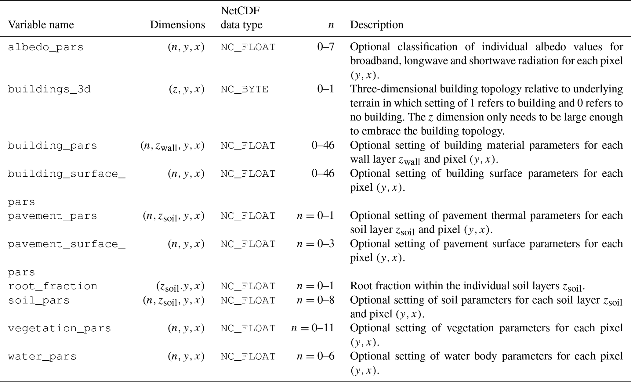
Based on the LOD1 classification of each surface pixel, the static driver allows overwriting all or selected parameters that were automatically set by the LOD1 input data (e.g. leaf area index (LAI), surface emissivity; see Tables A1–A7 in the Appendix). For each *_type field in LOD1 there is thus a respective *_pars field, representing LOD2 data (see Table 2). Note that LOD2 can only be used when simultaneously having specified LOD1 data. The *_pars fields then can contain fill values except for those locations where the data should be overwritten by LOD2 input data. Figure 1 shows this hierarchy exemplary for the LAI based on available data for Berlin, Germany. Additionally, LOD2 offers the NC_BYTE field buildings_3d, which can be used to specify three-dimensional building structures including overhanging structures, thoroughfares and bridges (see Sect. 2.5). Unlike for the other *_pars fields, the LOD1 data (i.e. buildings_2d) are not used if LOD2 data (i.e. buildings_3d) are present in the data. Furthermore, the field root_fraction can be set in order to specify a different vertical root distribution in the soil model of the parameterized vegetation in the land surface model.

Figure 1 Illustration of LOD1 and LOD2 hierarchy for the LAI around Berlin Ernst-Reuter-Platz. Panel (a) shows the determined vegetation_type classification, which involves automatic setting of an LAI for all pixels classified as vegetation (LOD1), shown in panel (b). Panel (c) shows LOD2 information of the LAI distribution transferred by the field vegetation_pars. Source: Sentinel-2, FIS Broker (dl-de/by-2-0: https://www.govdata.de/dl-de/by-2-0, last access: 26 October 2020) and © OpenStreetMap contributors 2018. Distributed under a Creative Commons BY-SA License.

Table 3 List of LOD3 variables that can be specified in the static driver file.

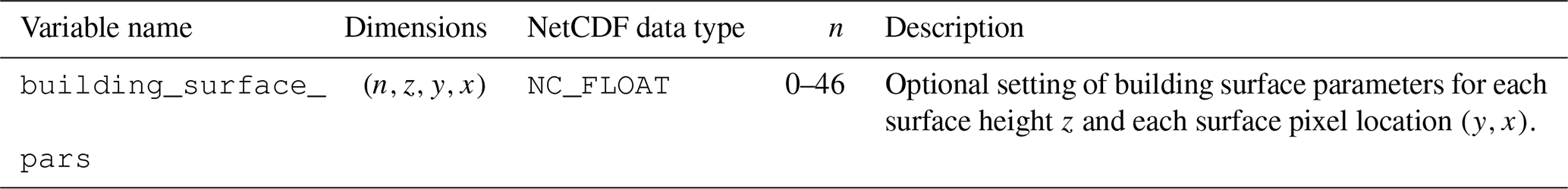
Table 4 List of LOD4 variables that can be specified in the static driver file.

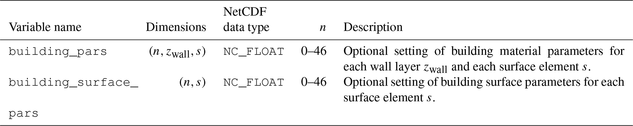
While LOD2 is limited to a localized setting of individual surface or material properties based on location (y,x) only, LOD3 and LOD4 settings (see Tables 3 and 4) allow an even more detailed specification of building parameters. Note that in LOD4, the input data no longer depend on the rastered PALM grid but are arranged in a one-dimensional array of size ns, where ns is the number of surface elements on the model domain. For each surface element, the user then has to specify the position of the surface element in the PALM domain space, i.e. $\left(z\right(\mathrm{1}:ns),y(\mathrm{1}:ns),x(\mathrm{1};ns\left)\right)$ as well as the orientation of surface elements in terms of azimuth and zenith angles (azimuth(1:ns) and zenith(1;ns), respectively) in one-dimensional fields.

Additionally, three-dimensional fields of leaf area density, LAD (lad), and basal area density, BAD (bad, implementation under development), as well as vertically distributed root fractions (root_fraction_resolved), and a tree ID (tree_id) can be used to set up resolved-scale plant canopies (see Sect. 5.3).

2.2 Georeferencing

Various model components such as the radiation parametrization, the representation of the Coriolis force or georeferencing of model output require information about the geolocation of the grid cells of PALM. Therefore, the static input file must contain information about the longitude and latitude, as well as the easting and northing UTM coordinates of the lower left corner of the model domain. Furthermore, reference height of the lowest model grid point as well as the rotation angle of the model domain must be provided, which is especially important to set up virtual measurement positions and trajectories within the model according to “real-world” measurements (Maronga et al., 2020). The required coordinate information must be given as global attributes in the NetCDF file.

2.3 Terrain height

To consider effects of elevation changes on the flow, the terrain height zt can be provided for each discrete (y,x) location in the model. Data gaps leading to fill values are forbidden. In case zt is not provided, the land surface is set up at zt=0 m.

The zt can be provided in absolute values (i.e. in metres above sea level) or in relative heights where, for example, its minimum value is already subtracted. If absolute values are used, PALM will subtract the minimum value within the domain itself to save computational grid points (no computations are needed within the soil). At this point we note that the original terrain height might be further processed and slightly modified by PALM to fulfil certain requirements, which is described in detail in Sect. 5.2.

2.4 Surface classification

In order to parameterize atmosphere–surface interactions, PALM needs to solve the energy balance at physical surfaces. To do this, several physical surface parameters such as heat capacity, roughness, albedo, emissivity, information about vegetation must be known. To allow for proper LOD1 initialization of material parameters and surface properties via predefined lists, PALM classifies all horizontal and vertical surfaces in the model according to their general type, e.g. whether it is a building or a vegetation surface. PALM considers four different types of surfaces: building, vegetation, pavement and water surfaces, while the surfaces are classified in a two-step approach. In a first step, grid points are flagged as atmosphere, building or terrain grid point. Surfaces which belong to a building grid point are automatically flagged as building surfaces, while surfaces which belong to a terrain grid point are flagged as land surfaces. In a second step, surfaces are further specified according to their respective type, which enables proper LOD1 initialization with predefined lists for material and surface properties. For this reason, input of building_type, vegetation_type, pavement_type and water_type is required. At each (y,x) location at least one of these types must have a non-missing value so that each surface element can be classified appropriately, either as a pavement, vegetation or water. It is also required that the given *_type matches the general classification into building and land surface; that is, at locations where buildings (see Sect. 2.5) are defined also building_type must be defined, while at land surfaces at least one of vegetation_type, pavement_type or water_type must be defined.

2.5 Buildings

Information on the location and height of buildings can be provided as two-dimensional buildings heights (buildings_2d, LOD1) or as a three-dimensional integer array (buildings_3d, LOD2), where each building (non-building) grid point is masked by 1 (0). At locations where no buildings are located, buildings_2d may contain fill values, while buildings_3d must not contain any fill values. In the LOD1 case, buildings are always mounted on the Earth's surface, and overhanging structures such as tunnels or bridges are not allowed, while in the LOD2 case also overhanging obstacles are allowed. In both cases, building information is given relative to the terrain height, and buildings are mapped onto the top of the terrain during model initialization, which is described in detail in Sect. 5.2. At this point we note that PALM can also consider bridges, which can be input as three-dimensional building structures but require a special treatment as further discussed in Sect. 5.2.

To distinguish between single buildings, for example, in order to map them accordingly onto the underlying terrain (please see Sect. 5.2) or to compute the energy demand of single buildings (Maronga et al., 2020), each building has an unique identification number (building_id) that must be given in the static input file at each (y,x) location where buildings_2d or buildings_3d is defined.

To solve the energy balance at building surfaces (Resler et al., 2017; Maronga et al., 2020), information on the type of the buildings must be provided. This includes information on various wall material, and surface properties must be known (e.g. wall thicknesses, heat capacities and conductivities, window and wall fractions, albedo), which depend on the individual construction parameters and the current state of building restoration. As much of this information is quite often unknown, buildings are classified into characteristic types in order to use default parameters. For this, buildings are classified according to their year of construction and its general usage (residential or office building). PALM provides lists of wall material and surface parameters for six building types (see also Table A2):

1. residential buildings built before 1950,

2. residential buildings built between 1951 and 2000,

3. residential buildings built after 2001,

4. office buildings built before 1950,

5. office buildings built between 1951 and 2000,

6. office buildings built after 2001, and

7. bridges.

At this point we note that building_type = 7 is exclusively used to identify bridges and to distinguish them from other three-dimensional building structures. The respective building_type must be provided for each discrete (y,x) location where building_2d or building_3d is defined. The provided wall and surface parameters are assumed to be valid for Germany but still have to be checked and likely changed for other building styles. Therefore, even though building parameters are difficult to aggregate in practice, PALM allows to one prescribe different types defined among a single building, e.g. to consider building extensions with different physical properties or different usage in case such information is available. In addition, to modify wall material and surface parameters at different (y,x) locations or even at single surface elements, building_pars or building_surface_pars, respectively, can be optionally provided.

2.6 Land surfaces

Beside the general classification via predefined parameter lists for each land surface type, physical surface parameters can be further specified with vegetation_pars, water_pars or pavement_pars, which can be optionally provided, as explained in Sect. 2.1.

2.6.1 Vegetation

PALM distinguishes between parameterized vegetation that is not resolved by the numerical grid (vegetation height smaller than the vertical grid spacing) and thus considered flat (e.g. short grass) and tall vegetation that can be partially resolved by the numerical grid, depending on the grid spacing used (e.g. shrubs or trees). Parameterized vegetation is considered within the energy balance solver for land surfaces, where the given vegetation_type defines the physical properties at the respective surface element (e.g. LAI, typical vegetation coverage of the soil, roughness, heat conductivity between the soil and the skin layer, emissivity). Currently 19 vegetation classes are defined in PALM, such as crops, shrubs, and forests (see Table A1). These can optionally be specified in more detail by vegetation_pars, which may contain missing values for single parameters and locations, and the respective properties are only updated and customized where they contain non-missing values: it is allowed to provide parameters only at locations where these are available. At parameterized vegetation surfaces, additional information concerning the root-area-density distribution (root_area_dens_s) within the soil can be optionally provided. If it is not provided it is taken from bulk parameter lists defined by the given vegetation_type.

In contrast to parameterized vegetation, resolved vegetation directly accounts for a sink term in the momentum equations (e.g. Kanani-Sühring and Raasch, 2015) and directly affects its surroundings via shading and three-dimensional reflections (Resler et al., 2017). To consider these effects in the model, information about the leaf area density (LAD) within the respective grid volumes is required and can be input via LAD, which is mapped on top of the underlying terrain. The leaf area density in the model is initialized at every location where LAD has non-missing and positive values; elsewhere it is set to zero.

2.6.2 Pavements

Pavement surfaces can be specified via pavement_type, which defines the surface and subsurface material properties via predefined parameter lists, which currently include 15 pavement types such as asphalt, concrete or cobblestone (see also Table A3). Pavement parameters are, for example, heat conductivities and capacities at different pavement layers, surface roughness lengths and emissivity. To further specify pavement parameters, pavement_pars and pavement_subsurface_pars can be optionally provided for defining surface and subsurface parameters, respectively.

Also, it is possible to provide additional input for street types and street crossings with street_type and street_crossing, respectively. The street-type classification (e.g. highway, local road, pedestrian road) can be used by PALM to parameterize traffic emissions within the embedded chemistry model, while both the street network and crossings may in the future be employed by the embedded multi-agent system for urban residents (Maronga et al., 2020). The crossings parameter therefore indicates the area where an agent is allowed to cross the streets.

2.6.3 Water bodies

Water surfaces can be specified via water_type, which defines the surface properties via predefined parameter lists (see Table A5 in the Appendix). Water types included are ocean, lake, river, pond and fountain. To further specify water surface parameters, water_pars can be optionally provided. Here the water temperature can specified, as well as z₀ and z₀,h. Emissivity of all water types is 0.99, and they belong to albedo_type 1, which is also specified in water_pars.

2.7 Soil classification

To consider the interaction of the land surface with the underlying soil at vegetation and pavement surfaces, a soil_type must be given at grid cells that are classified as vegetation or pavement surfaces, defining a list of default physical parameters for predefined soil types, based on the granularity of the soil (e.g. coarse, medium, fine or organic soil). soil_type can be given for different levels of detail. For LOD1, soil_type must be provided for each (y,x) location where vegetation or pavement is defined, assuming that soil properties are vertically homogeneous, while for LOD2 soil_type is given for each $(z_{\mathrm{soil}},y,x)$ location, with z_soil being the depths of the soil layers, in order to consider variations of soil properties also in the vertical direction. Respective soil properties are, for example, the van Genuchten parameter, hydraulic conductivity, volumetric soil moisture at saturation, field capacity at wilting point or the residual soil moisture. By default the soil layers have a depth of (from top to bottom) of 0.01, 0.02, 0.04, 0.06, 0.14, 0.26, 0.54 and 1.86 m, where pavement layers are by default assumed to cover the six uppermost layers (see also Table A4). Note that the vertical composition of materials used in road construction varies a lot and is usually unknown. The current implementation thus should be considered to be a first guess. To further customize physical soil parameters, soil_pars can be optionally provided either as LOD3 to provide vertically homogeneous parameters or as LOD4 to provide vertically heterogeneous parameters: each soil layer at each relevant surface element can be given individual physical properties. soil_pars may contain missing values and is only used to update the physical soil parameters at locations and for parameters that are non-missing: it is allowed to provide only single parameters at locations where this information is available.

2.8 Surface albedo

Information concerning the albedo for the different surfaces is already provided within the predefined parameter lists for building and land surfaces. However, more detailed information concerning the albedo_type (predefined list of broadband and spectral albedos for direct and diffuse radiation) or broadband/spectral surface albedos at each (y,x) location (albedo_pars) can optionally be provided.

3 Data sources

Masson et al. (2020) review various data sources for urban climate models at meso- and microscale. The requirement of a spatial resolution of 1–10 m for building-resolving simulations, being a key focus of PALM, reduces the available sources of data significantly. The most important sources are remote sensing, governmental/municipal data and open data, as they allow area-wide and automated preprocessing, while field surveys and manual mapping are only a practicable option for small areas of interest, e.g. of one building block in a city. Often, a combination of different sources is required to achieve a consistent coverage with detailed information for the entire area of interest.

The observation of the characteristics and dynamics of the Earth's surface by means of remote sensing has become increasingly important in recent years. In general, remote sensing approaches take advantage of the fact that material- or object-specific interactions occur between the surface and land cover type, on the one hand, and the electromagnetic radiation interacting with them on the other hand. This specific spectral signature or backscattering pattern can then effectively be used to identify and discriminate different surface and material types. Active imaging systems such as radar or laser scanners carry their individual radiation sources (Baghdadi and Zribi, 2016). The intensity and pattern of the backscattering then allows mapping the position, type and, in the case of laser scanners, height of surfaces and objects. This can be used to create digital surface models, e.g. based on the radar satellite TerraSAR-X at a global scale (Rizzoli et al., 2017) or at local scale using airborne lidar systems (Yan et al., 2015). Optical remote sensing makes use of the reflected radiation of the sun. There is a broad range of systems available, mounted on satellite platforms as well as airborne and UAV-mounted sensors. The selection of the sensor used depends on spectral characteristics, spatial resolution, availability for the area of interest and costs. Typical mapping tasks carried out with optical remote sensing are land cover mapping (e.g. Khatami et al., 2016; Wulder et al., 2018) and vegetation characterization (e.g. Verrelst et al., 2015). As the PALM model requires high spatial resolution for performing building-resolving simulations, the free and open Sentinel-2 satellite data are of interest as well as the data of commercial satellite constellations like Rapid Eye or World View. Additionally, false colour airborne imagery, with its very high spatial resolution, would be preferable if available for the right time of year.

Especially in developed countries, public authorities and agencies routinely collect a vast amount of geospatial data sets. The following focuses on the situation in Germany, because the selected study areas for the model development are located here. In Germany, available official data are hosted at different levels of agencies and departments (e.g. municipal, federal state, state, cadastral office). The accessibility of the data differs between the federal states and municipalities. In some federal states, such as Berlin, Hamburg, Thuringia or North Rhine-Westphalia, the data are easily accessible and downloadable and available through an Open Data Licence. These data sets are also regularly updated. The possibility to use additional official data depends on the purpose and costs. Municipalities interested in the resulting microclimate simulations usually provide their data on request for the purpose of a scientific study. The various German official data sets which are useful and available for most municipalities are addressed below. The cadastral data of ATKIS and/or ALKIS (Working Committee of the Surveying Authorities of the States of the Federal Republic of Germany, 2015) are used to estimate the building age when no detailed information for individual buildings is available. Additionally, the data set can be used for the localization of streets, public open spaces and water bodies. ATKIS and ALKIS are regularly updated every 1–3 years (depending on the land use category). The municipal parks and open-space departments host the data of the public green spaces and tree register. The latter is usually only available for trees on public land. Information about trees and green spaces on private property has to be derived from additional data sources. If a tree register is available it provides comprehensive information on tree species, age, height, and sometimes also crown and stem diameters. Building data are provided in the form of 3D building models in level of detail LOD1 (block buildings without exact roofs) or LOD2 (more detailed with roof parts). Since 2019, LOD2 building data have existed for all German states (Arbeitsgemeinschaft der Vermessungsverwaltungen der Länder der Bundesrepublik Deutschland, 2019a, b). However, accessibility and cost vary. A standardized data format for 3D city models is City Geography Markup Language (CityGML, Open Geospatial Consortium, 2012), an XML-based data format that can be used to describe the city in 3D at different levels of detail. Digital terrain, surface models or lidar data as well as aerial images are available at the departments of geoinformation or land survey administration at the federal state level in general. Aerial images are updated in a 2–5-year period to monitor the green volume development. For this purpose the images have to include the near-infrared band. The acquisition dates differ, dependent on their primary purpose, from early spring to summer and thus have a minimal or dense broad leave cover. Only the summer images present the phenological state needed to detect the tree canopy and with that the LAI and leaf area density (LAD). Soil data are available at the municipal level or at the state level in different scales from 1 : 10 000 to 1 : 200 000. Generally the municipal data cannot provide the full information required for a model parameterization so that additional data acquisitions and/or data fusion is needed.

Surprisingly, municipalities – at least in Germany – usually do not systematically collect spatially detailed information on the road network and pavement types. This gap can be closed using volunteered geographical information from the OpenStreetMap (OSM) project (OSM). One caveat of such crowd-driven data collection is that anybody can add any features and tags they think relevant, so no homogeneous data quality, completeness and adherence to a single standard can be guaranteed (Quinn and Bull, 2019). However Haklay (2010) and Graser et al. (2015) show that at least in western Europe OSM has a data quality on par with governmental sources. OSM can be utilized to add missing information to the government data (e.g. about road type, pavement type, bridges, pedestrian crossing points and water bodies).

Geodata can be stored in raster format, with a value for each raster cell or pixel. GeoTIFF is a common format supported by all geoprocessing software, but also the NetCDF supports geospatial information. Spatial data in vector format use the locations of point, lines and polygons with optionally attached attribute tables containing additional information on each spatial object. A commonly used vector format is the ESRI shapefile. Governmental data are often in vector format, as there are many attributes that describe an object. Remote sensing data are mainly raster data, as such data are recorded by the sensor in a regular grid.

4 Preprocessing of input data

Existing approaches to generating surface parameters for urban climate analysis, such as local climate zones (LZCs) (Stewart and Oke, 2012) (e.g. as implemented in the WUDAPT project, Ching et al., 2018) or the MApUCE tool (Bocher et al., 2018), focus on a coarser scale than PALM, as most urban climate studies do as well. The LCZ concept was considered not detailed enough to use it as basis for the generation of input data, as it provides indicator values per neighbourhood of 100–500 m, with no or little information on the configuration within the area. WUDAPT also recognizes that this is suboptimal for grid-based modelling applications and extends their research to mapping urban morphology parameters at finer resolution (30–100 m) using Landsat satellite data and the LCZ concept (Zonato et al., 2020). The simulation results of a numerical weather prediction model (NWP), in this case the WRF (Weather Research and Forecast) model, are according to Zonato et al. (2020) similar to lidar-derived data at the scale of 0.5 km and coarser. This is a very promising result, but as the spatial resolution of PALM is within the range of several metres, more detailed solutions have to be implemented for PALM. The project MApUCE (Bocher et al., 2018) provides a framework for generating urban indicators in a standardized way, in this case for all French municipalities at different levels of scale, from building to district. Although standardized mapping of indicators would be very helpful also for PALM, this system would need to be adapted thoroughly to allow for sub-building indicators that correspond to the grid cells of PALM instead of buildings or building blocks.

This section introduces a strategy and workflow for the selection and preprocessing of the input data sources for PALM 6.0. This is demonstrated for three cities in Germany with varying availability of input data: Berlin, Stuttgart and Hamburg. Despite the variety of data sources, it was aimed to automate the preprocessing for each layer as much as possible to ensure replicability and to handle the vast volume of data (0.5–1 TB per city, depending on target resolution and city area). This resulted in a collection of preprocessing scripts to which adaptations have been made for each of the three cities.

The municipal data of Berlin including the aerial imagery and 3D building model were retrieved from the Berlin Geoportal FIS Broker (https://fbinter.stadt-berlin.de/fb/index.jsp, last access: 19 December 2019). The municipal data including the aerial imagery and 3D city model Hamburg were retrieved from the Transparenzportal of the governmental offices in Hamburg (http://transparenz.hamburg.de/das-transparenzportal/, last access: 19 December 2019). The municipal data including the aerial imagery and 3D building model of Stuttgart were provided by the Landeshauptstadt Stuttgart for use in the [UC]² project (Scherer et al., 2019). Other sources of data are indicated directly in the text.

The scripts and programmes used to process the input data are currently not publicly available as they have some commercial and/or internal functionality. However we are currently in the process of maturing them and plan to make them publicly available with the PALM model in the future.

4.1 Terrain height

Active remote sensing systems are valuable sources to generate digital surface models. For the layers of Berlin, Stuttgart and Hamburg, products of two different active sensors are combined. Within the municipality boundaries, the terrain height is directly retrieved from the digital terrain model (DTM) data derived from airborne lidar data as provided by each of the municipalities in 1 m horizontal resolution (Berlin: https://fbinter.stadt-berlin.de/fb/feed/senstadt/a_dgm, last access: 19 December 2019; Hamburg: http://suche.transparenz.hamburg.de/dataset/digitales-hohenmodell-hamburg-dgm-16, last access: 19 December 2019). As this data set ends exactly at the municipal boundaries, a satellite-based yet coarser data set is added to provide terrain height for the surrounding areas, as PALM always requires a rectangular model region. In this case, the 30 m SRTM digital elevation model (DEM) was used. It is derived from the Shuttle Radar Topography Mission (SRTM) (Farr et al., 2007). For Stuttgart and Hamburg, the SRTM data set first had to be transformed from the global latitude–longitude geoid to the local German geoid. Subsequently, the SRTM DEM was clipped and resampled to the study areas with 1 m spatial resolution. Finally, the local terrain model and the SRTM terrain model were merged, with the local terrain model as the primary source. A feathering distance of 100 pixels was assigned for borders of the local terrain model to smooth any abrupt changes in height between the two data sets. The final terrain height data set for each of the three cities is shown in Fig. 2.

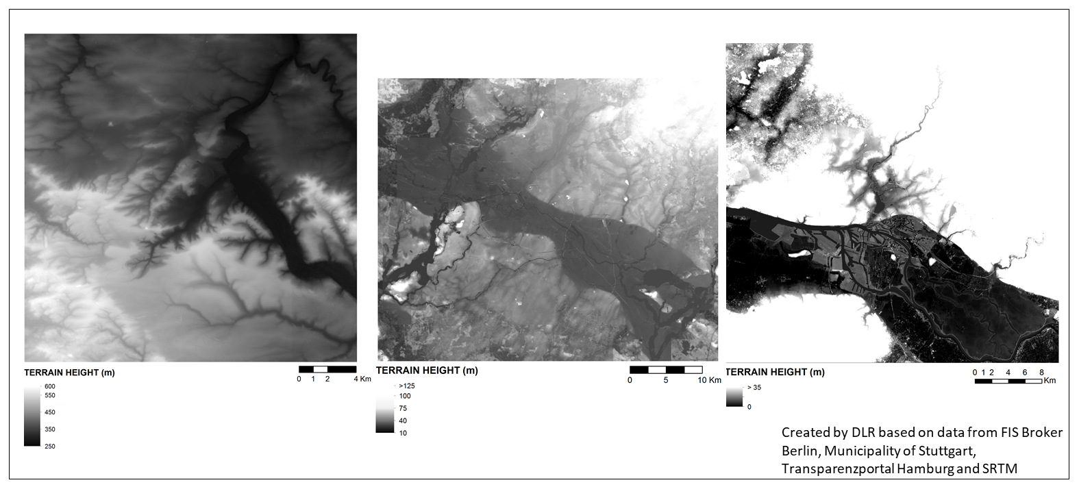
Figure 2 Terrain height for the study areas in metres above ground. From left to right: Stuttgart, Berlin and Hamburg. Sources: FIS Broker (dl-de/by-2-0: https://www.govdata.de/dl-de/by-2-0, last access: 26 October 2020) DOM, Municipality of Stuttgart, Freie und Hansestadt Hamburg, Landesbetrieb Geoinformation und Vermessung (2014) and SRTM.

4.2 Surface classification

PALM differentiates between building and land surface grid cells, where the land surface grid cells must consist of vegetation, pavements or water bodies (see Sect. 2.4). The first task within the surface classification is to map these four classes (buildings, vegetation, pavements and water bodies). The sections below describe how the according maps are prepared so that they can be written out into the static driver file. As soon as the four class rasters are available, possible gaps, which usually result from combining data sets from different sources or an artefact of rasterization, need to be filled, in at least one of the core classes (see Sect. 2.1). To achieve this, the layers were ranked according to their spatial reliability. For example, the building layer was preferred over the – often courser – vegetation layer. Secondly, extra secondary buffered input layers were generated where possible and used to fill in their primary layer for pixels where none of the primary layers or prior filled layers had valid data. For example this was necessary for roads, where exact information on roadside parking was not available, and thus the actual paved surface is wider than what would be expected from the road width. If there were still holes after all the filling iterations, they were filled with a prevalent reasonable value like bare soil, which is internally considered a vegetation_type and parameterized accordingly (see Table A1).

After the general surface classification is done, unique IDs for each of the buildings and bridges are generated to mark which pixels belong to the same object to support processing in PALM (see Sect. 5.2).

4.3 Buildings

For all the cities the building height, building type and building IDs were derived, which is described in the following sections.

4.3.1 Building height

For realistic simulation results of both the flow and the thermodynamic interaction with the urban canopy, it is essential to have the spatially resolved and correct building height. In Germany municipalities have 3D building outlines in LOD1 (block model) or LOD2, which contains differentiated roof structures and therefore allows spatially explicit height calculation for each pixel. For Hamburg and Berlin LOD2 data were available as CityGML (Open Geospatial Consortium, 2012) data (Berlin: https://fbinter.stadt-berlin.de/fb/feed/senstadt/a_lod2, last access: 19 December 2019, Hamburg: http://suche.transparenz.hamburg.de/dataset/3d-stadtmodell-lod2-de-hamburg4?forceWeb=true, last access: 19 December 2019), while in Stuttgart LOD2 building height data were provided as 3D triangulated irregular network (TIN). The developed approach to calculate the building height is a two-step approach. In a first step the 2D coordinates of all pixel centroids inside a single polygon as well as the 3D bounding box of the polygon are calculated using the algorithm from the GDAL library (GDAL/OGR contributors, 2019), which can cope with complex building geometries including, for example, inner courtyards. If the polygon is of single height, which is (nearly) always the case for floor polygons, this single height is used for all pixels. For each single centroid coordinate the 3D intersection between its vertical line and the plane of the polygon is calculated to get the height of the building at this position. The special cases in which the vertical line is inside or parallel to the plane (building walls directly passing through pixel centroids) are filtered. The calculated height values are capped to the z range of the bounding box. This is necessary to compensate for rounding errors in nearly vertical planes, which could lead to single intersects wrongly being near-infinite. The minimal and maximal height intersection is stored for each pixel. This approach works on the assumption that all the single polygons are planar polygons as defined in the cityGML standard (Open Geospatial Consortium, 2012), where all points of a polygon are in the same plane. However, for some single buildings in Berlin this assumption proved wrong as roof planes included single points from the walls of floors. These polygon errors were corrected where possible and otherwise removed from further calculations. Once all polygons have been processed the building height is calculated as the difference between maximum and minimum intersection. In a second iteration the same approach is repeated for all pixels that intersect the boundary of the polygons but where the centroid is outside the polygon. However, these height values are only used for pixels where no building height was calculated in the first iteration. This two-step approach guarantees that the extrapolation (with capping at the z range of the polygon) to coordinates outside the building footprint is only performed if no other polygons contain the centroid of this pixel. Therefore a higher building which slightly intersects the corner of a pixel will not interfere with lower buildings that cover the pixel while still removing a lot of single pixel holes with the other base layers (water, vegetation, pavement). This approach worked well for the city of Hamburg and Berlin, where some broken polygons had to be fixed beforehand. However in Stuttgart not all buildings had a closed floor polygon. Therefore in this case the terrain height was used as the lower boundary of the buildings. An example of the building height from the CityGML data of Berlin is given in Fig. 3 for the Reichstag building.

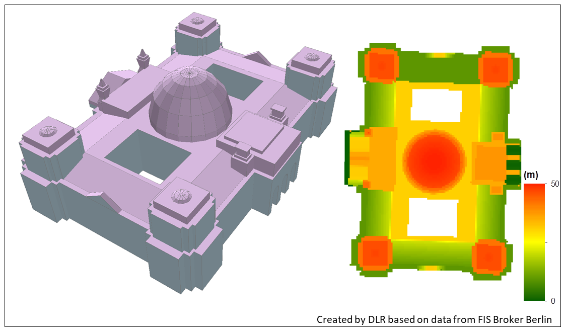
Figure 3 The 3D visualization of the CityGML data of the Reichstag building in Berlin (left) and the derived building height (right). Source: FIS Broker (dl-de/by-2-0: https://www.govdata.de/dl-de/by-2-0, last access: 26 October 2020) CityGML LOD2.

4.3.2 Building type

The building type describing the energetic properties of the buildings used in PALM is defined through a combination of building use and age (see Table A2). In Germany no cadastral information on restoration, facade changes and heat insulation actions for individual buildings is available so that the age of building construction used for building classification is often a rather poor proxy for the thermodynamic properties of buildings. Theoretically, energetic information on buildings exists in Germany, described in the energy performance certificate of each residential building. However, this information is not generally accessible. Currently, a research activity funded by the German Federal Ministry of Economic Affairs and Energy is developing a database on energetic characteristics of non-residential buildings (ENOB DataNWG; https://datanwg.de/home/aktuelles/, last access: 30 August 2020, in German). Thus, for small areas where high-quality simulations are desired, field surveys or drone surveys are still the best choice. For the large-area applications in this study however, this was not possible. Instead, we aimed at identifying the classes defined in Table A2. In Germany, the municipalities often maintain a building use database (e.g. in the ALKIS data sets). Usually these data are provided at building block level and therefore often contain mixed uses. For Stuttgart and Hamburg this data set was used to distinguish between residential and other building use (Hamburg: http://suche.transparenz.hamburg.de/dataset/alkis-ausgewahlte-daten-hamburg6?forceWeb=true, last access: 19 December 2019). The lookup table is given in Table B8. The cities of Hamburg and Stuttgart additionally maintain a database documenting the age of the building. This allowed the building type to be assigned with quite high reliability. For Berlin, a combined data set is available, where building blocks are categorized by use and building construction period at the same time (https://fbinter.stadt-berlin.de/fb/wfs/geometry/senstadt/re_isu5, last access: 19 December 2019). The lookup table to translate this information to building types is listed in Table B7. The building type maps for Stuttgart, Berlin and Hamburg are presented in Fig. 4.

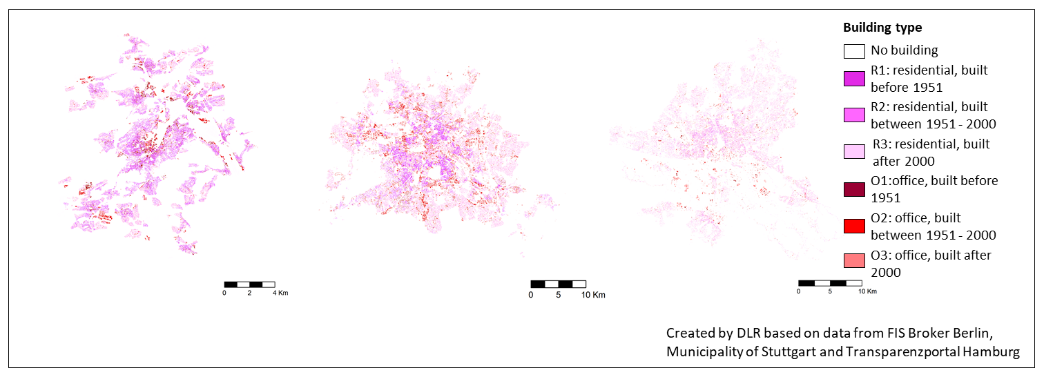
Figure 4 Building type maps of Stuttgart, Berlin and Hamburg (from left to right). Sources: FIS Broker (dl-de/by-2-0: https://www.govdata.de/dl-de/by-2-0, last access: 26 October 2020) ATKIS, Municipality of Stuttgart and Freie und Hansestadt Hamburg, Landesbetrieb Geoinformation und Vermessung.

4.4 Vegetation

PALM can handle very detailed information on the vegetation, as outlined in Sect. 2.6.1. In this study, the vegetation type was determined as well as vegetation on roofs and several characteristics of trees. As an area-wide approach, satellite or airborne imagery provides accurate information on the location of the vegetation. Such remote sensing data can also provide estimates for some vegetation characteristics but not all required by PALM. Luckily, in Germany there is a huge amount of information available from municipal data that cannot be retrieved with remote sensing data alone. Also, open data such as OSM and other citizen science projects can provide valuable information on the urban vegetation. Therefore these sources are all combined to derive as complete input data for PALM as possible.

4.4.1 Vegetation type

For the vegetation type layer, municipal data were used in the three demo cities, including ALKIS (Berlin) and the Biotope Cadastre (Hamburg). For Stuttgart, such municipal data were not available; thus OSM was used as the main source here. Subsequently, gaps were filled with data from Corine Land Cover (CLC, European Union, 2017), which was especially the case for areas outside the municipal borders. Missing data and gaps in the layer between vegetation and other features are filled using aerial colour and infrared images (CIR images), using a threshold on the normalized difference vegetation index (Rouse et al., 1974) (NDVI) to differentiate between grass and trees. The NDVI can be calculated by Eq. (1):

$$\begin{array}{}\text{(1)}& \text{NDVI}={\displaystyle \frac{{\mathit{\rho }}_{\text{nir}}-{\mathit{\rho }}_{\text{red}}}{{\mathit{\rho }}_{\text{nir}}+{\mathit{\rho }}_{\text{red}}}},\end{array}$$

where ρ_nir is the reflection in near-infrared part of the spectrum and ρ_red the reflection in the red part of the spectrum. Pixels with a NDVI between 0.2 and 0.42 were assigned to vegetation class 3 (short grass), and pixels with NDVI values above 0.42 are assigned to class 7 (deciduous broadleaf). The thresholds have been selected empirically based on the available airborne imagery. Depending on sensor, date, time of day, weather at time of the acquisition or preprocessing options, optimal thresholds might differ for other cities.

For the different data sources lookup tables have been created to map the classes of OSM (https://planet.openstreetmap.org/, last access: 19 December 2019; Table B2), CLC (Table B2) and the biotope maps of Hamburg (http://suche.transparenz.hamburg.de/dataset/biotopkataster-hamburg1?forceWeb=true, last access: 19 December 2019; Table B3) to the vegetation types of PALM. The main classes of ALKIS already directly match the PALM vegetation types. The vegetation type layer was created together with other layers as described in Sect. 4.2. As a result, the vegetation type layer is empty in locations of streets and water bodies. The result is shown in Fig. 5.

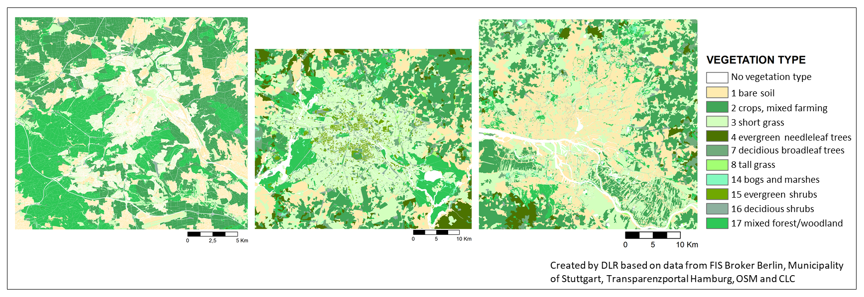
Figure 5 Vegetation type. From left to right: Stuttgart, Berlin and Hamburg. Sources: FIS Broker (dl-de/by-2-0: https://www.govdata.de/dl-de/by-2-0, last access: 26 October 2020), Municipality of Stuttgart, Freie und Hansestadt Hamburg, Landesbetrieb Geoinformation und Vermessung, European Union (2017) and OpenStreetMap.

4.4.2 Vegetation on roofs

Intensive and extensive green roofs are detected using municipal 10 to 20 cm ortho near-infrared (CIR) images in combination with the building footprints for the cities of Berlin and Stuttgart. The majority of green roofs are extensive green roofs which mostly have a shallow substrate of 100 to 250 mm and are usually planted with low-maintenance water-stress-tolerant mosses, succulents, herbaceous plants and grasses. Intensive green roofs are rarer and mostly belong in the category of recreational rooftop parks. They consist of gardened landscape of grass, shrubs and even small trees (FLL, 2002). The percentage of green roof vegetation is aggregated for each building roof pixel. The mostly very extensive green vegetation on roofs is detected by analysing the NDVI (Eq. 1). The NDVI utilizes the unique characteristic of photosynthetic active vegetation to absorb light in the red part of the spectrum and emit it in the near-infrared, making vegetation distinguishable from other materials. Minimum and maximum thresholds on the NDVI were determined empirically from the aerial images, as the thresholds depend on the vegetation conditions during image acquisition, the preprocessing and colour enhancing steps during the creation of the images, as well as the sensor systems used aboard the plane. Therefore the thresholds vary between cities. The lower threshold (0.2 in Berlin, 0.06 in Stuttgart) distinguishes the extensive vegetation from bare roofs, while the upper bound (Berlin 0.4, Stuttgart 0.25) is used to distinguish extensive from intensive vegetation and remove these from the green roof vegetation. The intensive vegetation is removed as it was mostly caused by trees growing over the roof, rather than on the roof or by potted plants. Figure 6 also shows the problems associated with merging information from different sources, as the aerial images do not fully compensate for the perspective of oblique sideways acquisition: especially for higher buildings, there is a shift between the building outline and where it is recorded in the image. This can lead to erroneous vegetation along the borders of buildings, both over- and underestimating the vegetation. In Hamburg no near-infrared aerial data were available at the time to create the green roof layer.

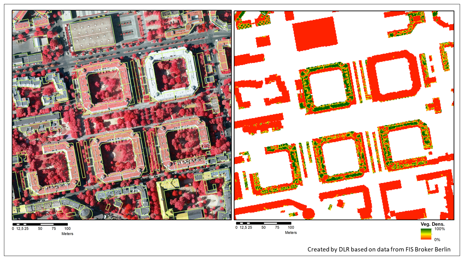
Figure 6 The 10 cm CIR image of a small subset of Berlin on the left, overlaid with the building outlines in yellow. The perspective offset between the orthoimage and the building outlines is especially pronounced for the high round building at the bottom. The resulting vegetation density map for PALM at 1 m resolution is shown in the right illustration. Sources: FIS Broker (dl-de/by-2-0: https://www.govdata.de/dl-de/by-2-0, last access: 26 October 2020) CIR Luftbilder.

4.4.3 Trees

To resolve tall vegetation (i.e. trees), a range of additional parameters have to be specified that support the generation of leaf area density (see Sect. 5.3). In this study, we aimed at deriving tree height, crown diameter, trunk diameter, tree type and tree species, as well as the leaf area index, which is described in Sect. 4.4.5. While tree height and crown diameter could be derived from lidar data (Fassnacht et al., 2016), the other parameters are very difficult to acquire without extensive field surveys. Luckily, many German cities have tree cadastres, where they store exactly these characteristics to support the maintenance of public trees. Such data sets were available for Berlin, Hamburg and Stuttgart, although the Stuttgart data set only included tree species. Please note that in these municipal data sets only public trees (e.g. along public roads or in parks) are included. Private trees (e.g. in gardens) are missing. If no additional sources are available (e.g. as described in Sect. 4.4.4), this means that the uncertainty increases of representing real-world conditions correctly in PALM.

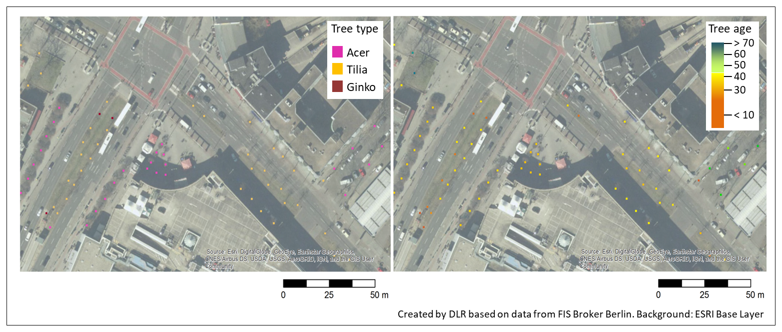
Figure 7 Tree species (left) and tree age (right) of municipal trees in Berlin source: FIS Broker (dl-de/by-2-0: https://www.govdata.de/dl-de/by-2-0, last access: 26 October 2020) Baumkataster.

To prepare the data for PALM, lookup tables for tree type and species were created, which contain all species and types of trees recorded in the three cities. A class number was assigned to each type and species and then joined to the attribute table of the tree cadastre shapefile. Varying spellings for the same type or species were taken into account and assigned the same value. For the attributes age, height, trunk diameter and crown size all numbers were checked for plausibility and corrected (typos, wrong unit, shifted columns). The resulting point shapefiles were converted to raster (geoTIFF) and then NetCDF. Figure 7 shows exemplary tree type and age maps for a subset of Berlin.

4.4.4 Vegetation patch

Instead of providing tree properties of single trees, it is also possible to provide the information on the high vegetation in an area-wide manner, as vegetation patches. This is practical, as the tree data sets that were available only cover public trees. Information on all other trees needs to come from another source. Suitable sources are lidar data or to some extent also (governmental) forestry data. Not all cities in Germany provide access to lidar data sets, but for Berlin we could use a lidar-based data set as well as forestry data. The city of Berlin provided a vegetation height map (http://www.stadtentwicklung.berlin.de/umwelt/umweltatlas/i509.htm, last access: 19 December 2019), which included the height for all vegetated areas, thus including both public and private trees and shrubs as well as vegetation in parks. For forest vegetation outside Berlin, the Umweltatlas of Berlin (Environmental Atlas) provided information on average tree height, age, type and trunk diameter at breast height for each forest lot as a shapefile (http://www.stadtentwicklung.berlin.de/umwelt/umweltatlas/ib504.htm, last access: 19 December 2019). The lidar-based vegetation height and the vegetation height of the Umweltatlas were merged, using the lidar-based vegetation height as the primary data set. The resulting map for the vegetation patch height is shown in Fig. 8.

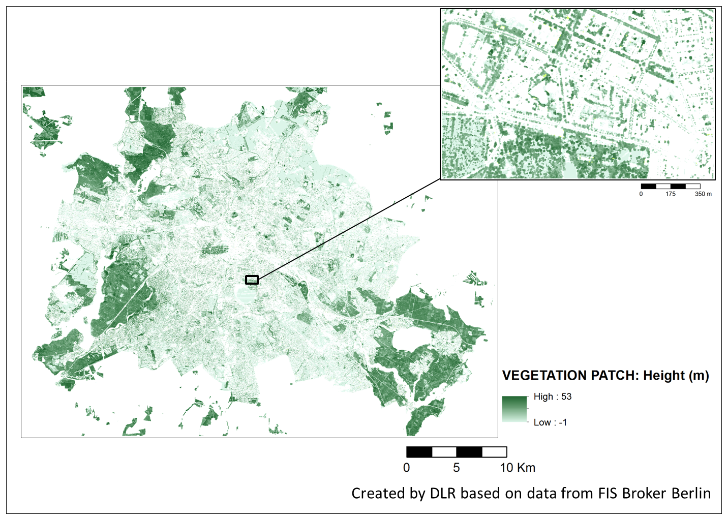
Figure 8 Height of vegetation patches in Berlin. Source: FIS Broker (dl-de/by-2-0: https://www.govdata.de/dl-de/by-2-0, last access: 26 October 2020) Umweltatlas.

4.4.5 Leaf area index

The LAI is an important parameter for the generation of the LAD, which is described in Sect. 5.3. LAI is defined as square metres of leaf area per square metre of ground area and is therefore dimensionless. The LAI varies largely over the phenological cycle. Therefore it is important to approximate the state of the vegetation of the day to be simulated in PALM as best as possible in the input data. Remote sensing is the most suitable data source for representing this temporal variation. Field measurements on the ground only sample single trees, but with area-wide remote sensing data an estimation of the LAI of larger area is possible. Typical approaches for LAI estimation make use of vegetation indices in combination with empirical relationships between a vegetation index and LAI. As only multispectral remote sensing imagery was available for this study, an NDVI-based method was selected, making use of Sentinel-2 optical satellite data. Depending on the study area up to three Sentinel-2 image tiles (so-called image granules) had to be combined to create a complete coverage of the city area. This is only possible if cloud-free image granules of the same or close dates are available. The aim was to create cloud-free coverages for each season. Using data of the year 2017, cloud-free images of Berlin, Stuttgart and Hamburg could be created for spring and summer, as well as an additional winter image for Hamburg and an autumn image for Stuttgart.

Using the TimeScan processing chain (Esch et al., 2018) the NDVI was derived for all Sentinel-2 scenes. For each date range, an NDVI mosaic image of the study area was created using GDAL tools (GDAL/OGR contributors, 2019). Then the LAI is calculated using an IDL ENVI algorithm (Interactive Data Language and Exelis Visual Information Solutions, Boulder, Colorado) for each study area and date. For this, an empirical relationship between NDVI and LAI is used as documented by Wang et al. (2005) for deciduous forests. All non-vegetation pixels are set to 0 (vegetation mask). As the spatial resolution of Sentinel-2 is 10 m, the required resolution of 1 m is reached by resampling the LAI map using a bilinear resampling method. For a subset of Hamburg the estimated LAI is presented in Fig. 9 for spring, summer and winter.

Figure 9 LAI for a subset of Hamburg in winter (14 February 2017, left), spring (20 April 2017, centre) and summer (23 August 2017, right).

4.5 Pavements

As a source for the pavement, layer airborne hyperspectral would be very useful. Such spatially and spectrally detailed data would allow a differentiated classification of urban surface materials (van der Linden et al., 2019; Roessner et al., 2001). However, due to its experimental nature, hyperspectral data are rarely available for whole cities. Therefore, OSM data were used instead. OSM contributors not only mapped road features but often also indicated the surface materials. As the contributors do not apply homogeneous labels, a lookup table was created to map all the materials listed in OSM for the test cities to the PALM pavement types. If no surface material is indicated, default materials are assumed for each road type (Table B5). Using another lookup table, the materials were matched to the pavement types listed in the PIDS. As the roads in OSM are line features, each road is buffered with the width or, if not available, a default width for that type of road (Tables B5 and B6). After rasterization, the data set is checked for gaps between pavement type, vegetation type, buildings and water. Gaps are filled with the road pavement type by applying a larger buffer (3× the listed diameter) on the road lines. An example of the resulting pavement type raster map is shown in Fig. 10.

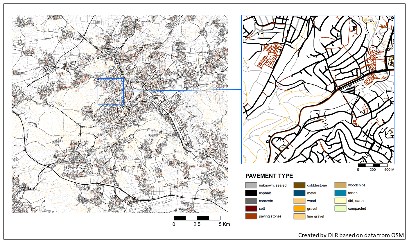
Figure 10 Pavement type of Stuttgart. Source: OpenStreetMap.

4.5.1 Street type and street crossings

For the street types and street crossings, data from OSM are used. Street types directly use the classes specified in OSM and are assigned to the road grid cells. If multiple road types cover a pixel, the highest class is assigned. Thus a motorway would have precedence over, for example, a primary road. A street crossing flag is assigned to all parts of the streets that are marked in OSM as a street crossing. As this label is a point feature, all grid cells in a buffer of 15 m around each crossing point are flagged as a crossing. At the moment, input data for street_type and street_crossing are used by PALM's embedded chemistry model (see Maronga et al., 2020; Khan et al., 2020) to parametrize emissions of chemical compounds during the diurnal cycle.

4.6 Water bodies

Multispectral remote sensing is a suitable tool to map water bodies (Ma et al., 2019), but at the high spatial resolution required for building-resolving simulations, the spatial resolution of most satellite data is not sufficient. Also aerial images usually do not provide enough (and calibrated) spectral bands, to distinguish smaller water bodies like fountains or rivulets. Therefore, also in this case OSM was used as the primary source for the demo cities. Unfortunately, it turns out OSM is incomplete regarding water bodies. Therefore the data sets were merged with CLC data for Stuttgart and ALKIS and the Biotope Cataster in Hamburg. Lookup tables were created to assign a PALM water class to each water feature in the different data sets (see Tables B9 and B11). ALKIS polygons are sorted into water types that match the PALM water types (Working Committee of the Surveying Authorities of the States of the Federal Republic of Germany, 2015). Also CLC contains classes that map directly to the PALM water types (European Union, 2017). After the data sets were merged, for Stuttgart and Berlin several important water bodies had to be added manually. The final water type maps for the cities of Stuttgart, Berlin and Hamburg are presented in Fig. 11.

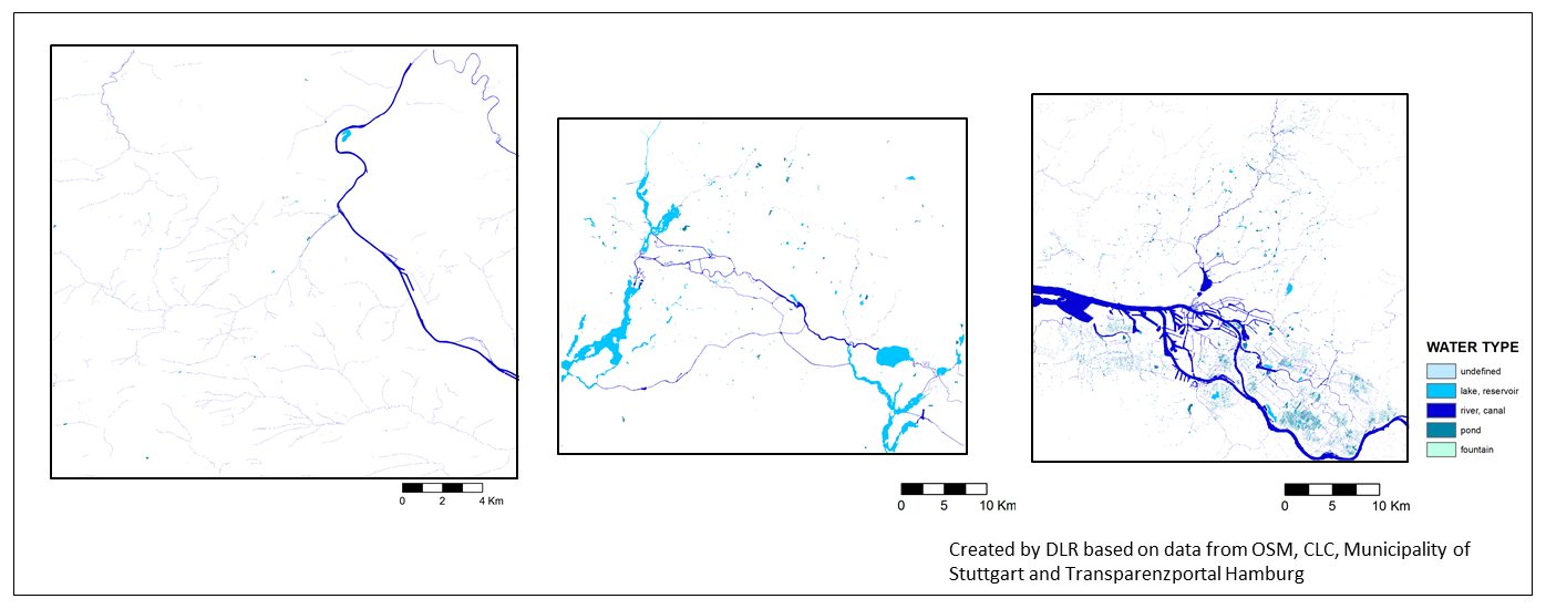
Figure 11 Water type of Stuttgart, Berlin and Hamburg (from left to right). Sources: Municipality of Stuttgart, Freie und Hansestadt Hamburg, Landesbetrieb Geoinformation und Vermessung, European Union (2017) and OpenStreetMap.

4.7 Soils

As soil data are difficult to acquire, especially at resolutions less then 10 m, a horizontally and vertically homogeneous soil type distribution (with soil_type = 1, coarse soil texture) is assumed in this study: the physical properties of the soil are identical all over the model domain. Further information on the initial state of the soil moisture and temperature at each pixel can be given as LOD0 via Fortran namelist input or as LOD1 input given in the dynamic input file (Maronga et al., 2020). The respective soil information can be, for example, taken from mesoscale models such as COSMO or WRF, which is described in a separate follow-up paper (Kadasch et al., 2020).

5 Preparation of input data for PALM

In this section we discuss PALM static driver generator, the generation of three-dimensional vegetation data in terms of LAD and basal area density (BAD) fields from two-dimensional information as part of the static driver, as well as the internal topography processing which is required to ensure all PALM requirements on the terrain data are met. Note that the netCDF interface routine in PALM has undergone several improvements since the official release of PALM 6.0. In the following, we will thus describe the status quo for PALM 6.0 in revision 4311.

5.1 Using the PALM static driver generator

In order to enable the user to create static drivers for complex scenarios, the Python 3.0-based preprocessing tool palm_csd (short for PALM create static driver) is shipped with PALM. The tool comes with a comprehensive library with netCDF functions and utility routines that can also easily be plugged into user-specific Python codes, and which take care of the correct formatting of static driver files that comply with PALM's netCDF interface. palm_csd itself, however, is a wrapping and compiling tool, which compiles static drivers based on already processed and rasterized geospatial data in netCDF format, but it cannot process other geospatial file formats (e.g. GeoTIFF or shapefile). At the moment, it is thus up to the user to process such data manually and provide palm_csd with PIDS conform NetCDFs. Currently, input data for palm_csd are available for the cities of Berlin, Hamburg and Stuttgart in Germany, for which input data were processed based on the data sources outlined in Sect. 4, but the user is free to provide their own data to be processed by palm_csd. Note that while data for Berlin and Hamburg are freely available for the general public, data for Stuttgart are restricted to be used within the [UC]² project. During the preprocessing of the data for Berlin, Hamburg and Stuttgart, it was aimed to automate the preprocessing steps as much as possible by implementing the geoprocessing in scripts and reduce manual processing in GIS software. In the next phase of [UC]² it is planned to develop a preprocessing tool that will support users to generate the input data in PALM conform formats.

palm_csd is steered via a configuration file in which input files, basic settings and default values are defined. Once this configuration file is set up, the user can generate their own static driver files that include correct metadata and possibly georeferencing (depending on suitable input data) for PALM and that will also be written to PALM's output data for postprocessing and visualization.

We plan to extend palm_csd for generic and academic set-ups as well as with a graphical user interface in near future. Moreover, we plan to implement a comprehensive checking routine to ensure compatibility with PALM, which is currently done within PALM itself.

5.2 Internal topography processing

During the initialization of PALM, the provided topography data, encompassing terrain height and buildings, are further processed and could possibly be slightly modified (e.g. to fulfil numerical requirements or to reduce the use of computational resources).

The model surface in PALM is internally defined at z=0 m. Therefore, in a first step, PALM internally computes the relative terrain height $z_{\mathrm{t}}^{\prime }=z_{\mathrm{t}}-z_{\mathrm{t},\min }$, where z_t,min is the minimum terrain height occurring within the model domain. Thus, the minimum $z_{\mathrm{t}}^{\prime }$ coincides with the model surface at z=0 m, and the first vertical grid level has at least one grid point that lies within the atmosphere. For instance, if z_t is given in metres above sea level and we would use this without any further processing, many grid points may lie below the Earth surface, being a waste of computational resources without providing any additional value. In the case of a nested simulation set-up with a root domain and various child domains, z_t,min is calculated as the minimum terrain height over all domains, in order to have the same reference height for all model domains and avoid artificially induced elevation changes at the domain borders between the parent and the child models.

In the following, $z_{\mathrm{t}}^{\prime }(y,x)$ is projected onto the discrete grid, while all grid points are flagged as terrain that are located below $z_{\mathrm{t}}^{\prime }(y,x)$, as illustrated in Fig. 12 by the dashed black line.

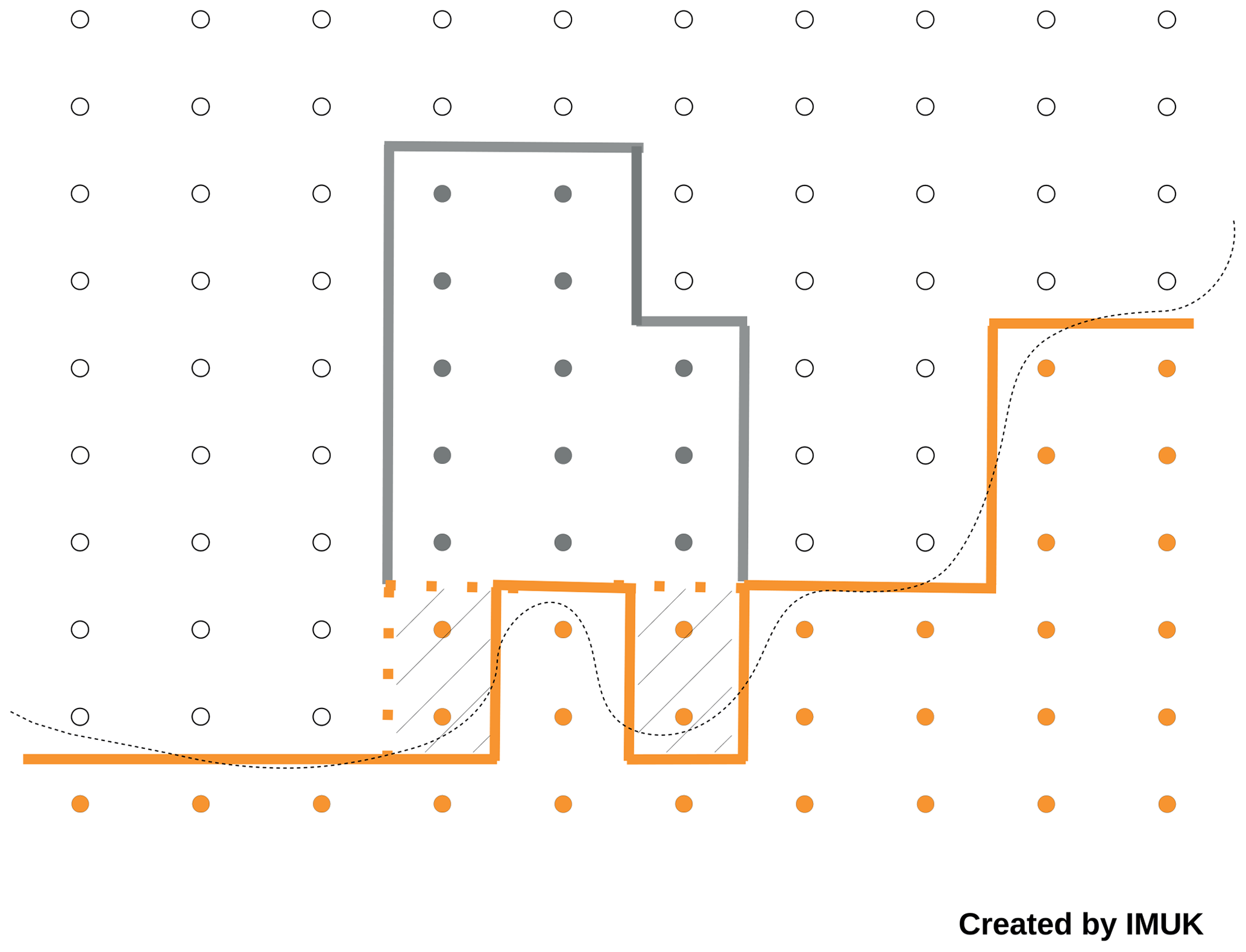
Figure 12 Schematic illustration on how buildings are mapped onto the underlying terrain. The thin dashed black line indicates the original relative terrain height $z_{\mathrm{t}}^{\prime }$. Solid orange lines indicate the original discrete terrain surface, while dashed orange lines indicate the resulting discrete terrain surface after the terrain is flattened below buildings, as indicated by the hashed areas. Grey solid lines indicate building surfaces. Orange and grey coloured points indicate terrain and building grid points, respectively, while non-filled points indicate atmospheric grid points.

In a second step buildings are mapped on top of the discrete terrain, which is illustrated schematically in Fig. 12. Especially when the underlying terrain is not flat but elevation changes occur below a building, roof shapes should be maintained so that buildings cannot be simply mapped on top of $z_{\mathrm{t}}^{\prime }$. Hence, the underlying terrain below a single building (which is identified by its building_id) is padded up to the level of the highest $z_{\mathrm{t}}^{\prime }(y,x)$ within the building-covered area with respective building_id: $z_{\mathrm{t}}^{\prime }(y,x)=max\left(z_{\mathrm{t}}^{\prime }\right(y,x){)}_{ID}$; i.e. the terrain below the building is flattened (please see the hashed areas in Fig. 12). This guarantees that building and roof shapes are maintained even at steep slopes. However, an exception is made for bridges (identified by building_type = 7), where buildings_3d is directly mapped on top of $z_{\mathrm{t}}^{\prime }$. Flatting the terrain below the bridge to the highest terrain height (often the top of the levee) would otherwise introduce barrier-like topography structures.

While buildings are mapped onto the terrain, grid points that lie within buildings and below terrain are internally flagged, in order to classify building or land surfaces during the surface initialization (see Sect. 2.4). The padded grid points below buildings will be not flagged as building but as land surfaces, while these artificially introduced vertical land surfaces will be initialized using the given vegetation_type or pavement_type at the adjacent grid cell.

After the topography is projected onto the discrete grid, it may contain single pixel cavities or chimney-like holes that are only resolved by one grid point. Due to numerical issues, such one-grid-point cavities must be filtered. In many cases these filtered cavities are building courtyards that are resolved by only one grid point. In this case, the courtyard grid point, which might be originally given (e.g. a vegetation_type), is internally flagged and reset to a building grid point while it obtains building_type, building_id and, if available, building_pars from the nearby building grid point. Hence, we filter such one-grid-point cavities during the model initialization, meaning that small differences might occur between the final building and terrain geometry in the model and the provided one in the static driver.

5.3 Generation of three-dimensional leaf area density and basal area density fields

When using PALM at very high resolution of the order of 1 m, vegetation like tall shrubs or trees cannot be represented by common parameterizations that assume the vegetation canopy to be flat and represented, e.g. by a roughness length. Under such conditions, PALM employs a plant canopy model in which high vegetation can be represented in terms of three-dimensional LAD fields. As geospatial data usually do not yield any exact three-dimensional information, three-dimensional LAD and BAD fields must be estimated from two-dimensional data and other data sources. In order to allow for a pseudo-automated generation of LAD and BAD fields, palm_csd comes with two different routines for creating vegetation canopies: a routine for single trees as often found in urban environments and a routine for creating vegetation canopies like forests and parks. In the following we will outline the basics of both routines. Note, however, that both routines are still in experimental stage and will be further developed and evaluated in the near future. In the following we will thus describe the status quo of these routines.

5.3.1 Generation of leaf area density and basal area density fields for single trees

Single trees, whose growth is seldom affected by other trees or obstacles, can be characterized in terms of three-dimensional LAD and BAD fields by a limited number of parameters. In palm_csd these are the maximum tree height, crown diameter, crown shape, trunk diameter, height of the maximum LAD value and the aspect ratio of tree crown diameter to tree crown height (see Figs. 13 and 14). In German cities, several of these parameters are available from tree cadastral register data. For example, for Berlin more than 400 000 municipal trees are collected in a publicly available database including information about tree species, tree height, crown diameter, stand age and trunk diameter.

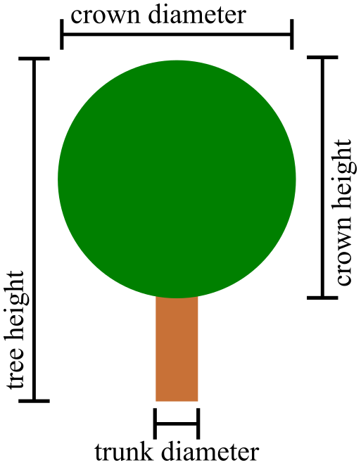
Figure 13 Schematic view of the parameters for a spherical tree shape through which the three-dimensional structure of trees is constructed in the single-tree canopy generator.

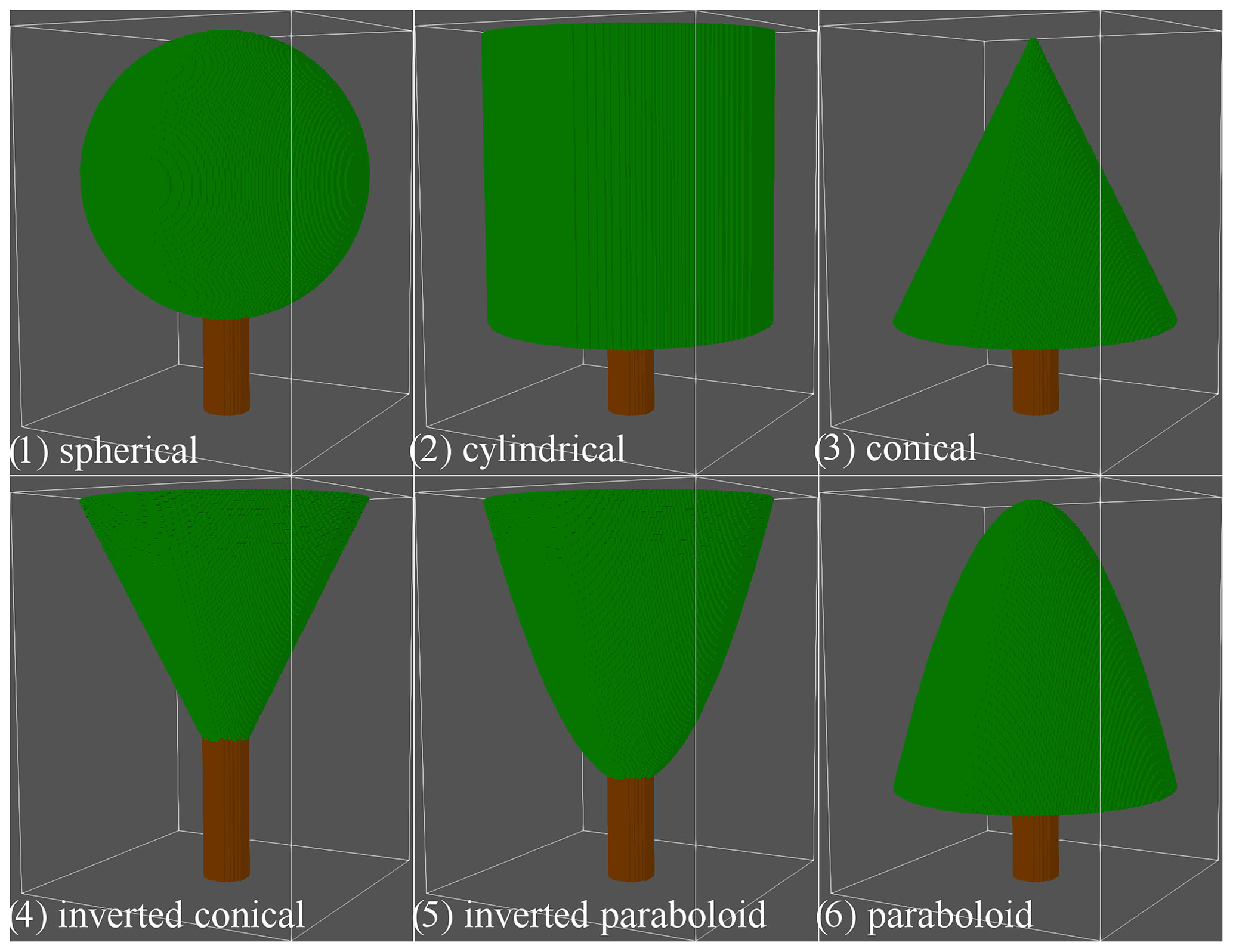
Figure 14 Overview of tree shapes available in the single-tree canopy generator. Green surfaces represent the foliage while brown surfaces represent the tree trunk. The shown sketches were created for a raster size of 0.05 m using a tree height of 8 m, a crown width of 6 m, a crown height to width ratio of 1 and a trunk diameter of 1 m.

Table 5 List and average properties of the most common street trees in Berlin.

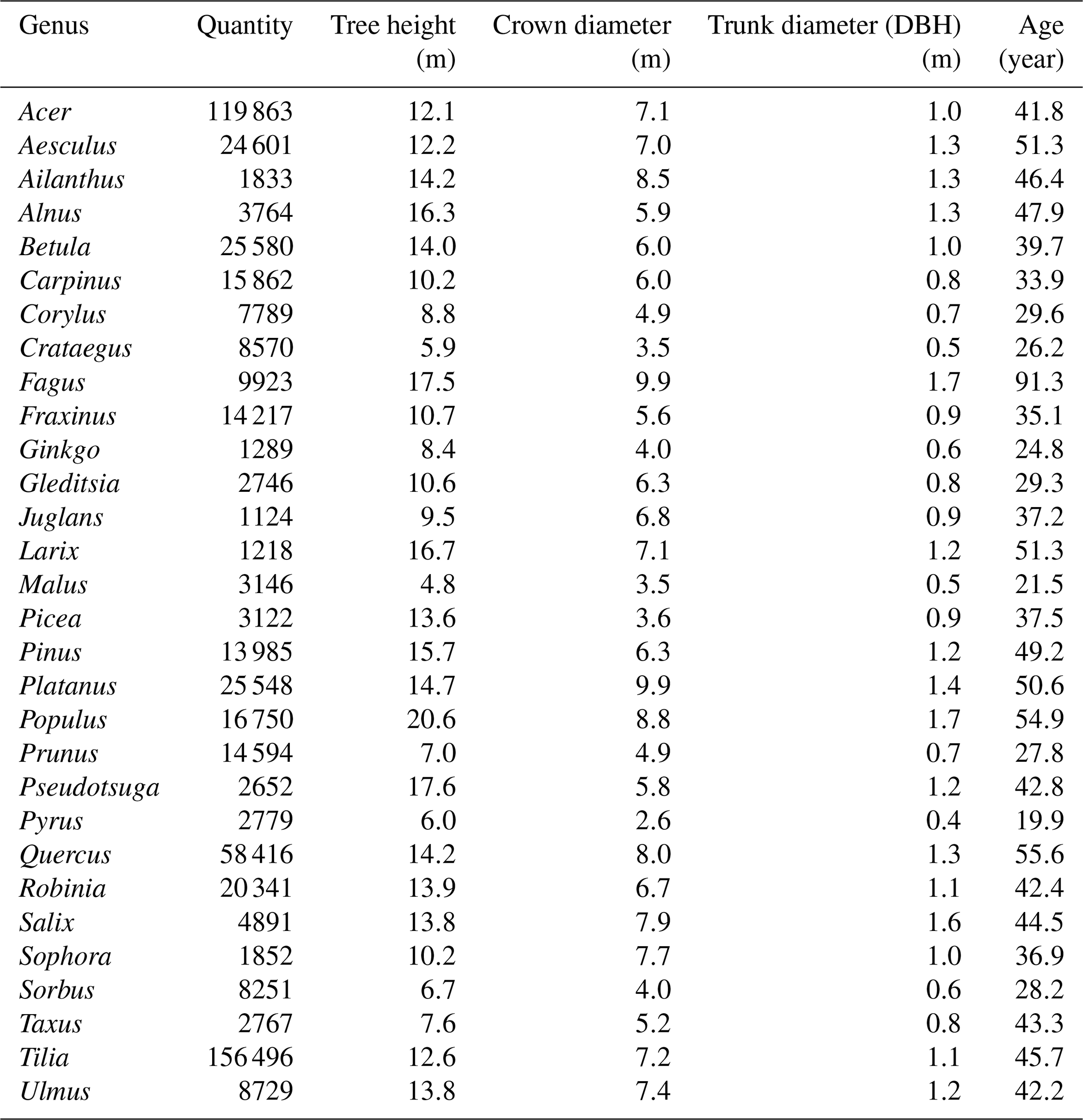
The single-tree canopy generator in palm_csd is called for each individual tree, and the following information is passed to the generator: location (y,x) of the tree centre, tree type (i.e. genus), tree height, LAI, crown diameter and trunk diameter at breast height. If one or more of these parameters is not provided, a default value from a lookup table (see Table 5) is used, which was generated based on averaging each tree parameter for each tree type in the Berlin tree database. This lookup table also includes default values for the tree shape, the ratio between crown height to crown width, LAI values for summertime and wintertime, and the height of the LAD maximum. Note for some of the latter parameters only dummy values are currently available (crown height to width ratio, LAI, height of LAD maximum), and more effort will be needed to fill this table with reasonable data. The tree generator allows for six different tree shapes, which are shown in Fig. 14 and which cover most of the commonly observed shapes for single trees. The generation of a three-dimensional LAD volume then consists of two steps. First, the volume covered with leaves is determined based on the shape, crown diameter, tree height and the ratio of crown height to width. Second, the three-dimensional LAD field is created using an exponentially increasing LAD towards the outer shell of the foliage. This approach is based on the empirical finding that sunlight is absorbed when entering the foliage, resulting in decreasing production of leaves.

Calculation of three-dimensional BAD fields is available using an interim solution, where the BAD field is calculated from the given trunk diameter, which is taken as a constant up to the centre of the tree crown. At the moment, the canopy generator only allows one to treat each grid volume as either (impermeable) stem or no stem. The representation of grid volumes partially covered by trunks is thus not possible at the moment. BAD values within the crown canopy is calculated as

$$\begin{array}{}\text{(2)}& \text{BAD}=\mathrm{0.1}\cdot \left(\mathrm{1}-\text{LAD}\right),\end{array}$$

which reflects increasing BAD towards the centre of the crown. An example of both lad and bad fields for an idealized spherically shaped tree is shown in Fig. 15. Note, however, that PALM currently only supports LAD so that only the foliage is read from the static driver. The import of BAD data will be realized in near future.

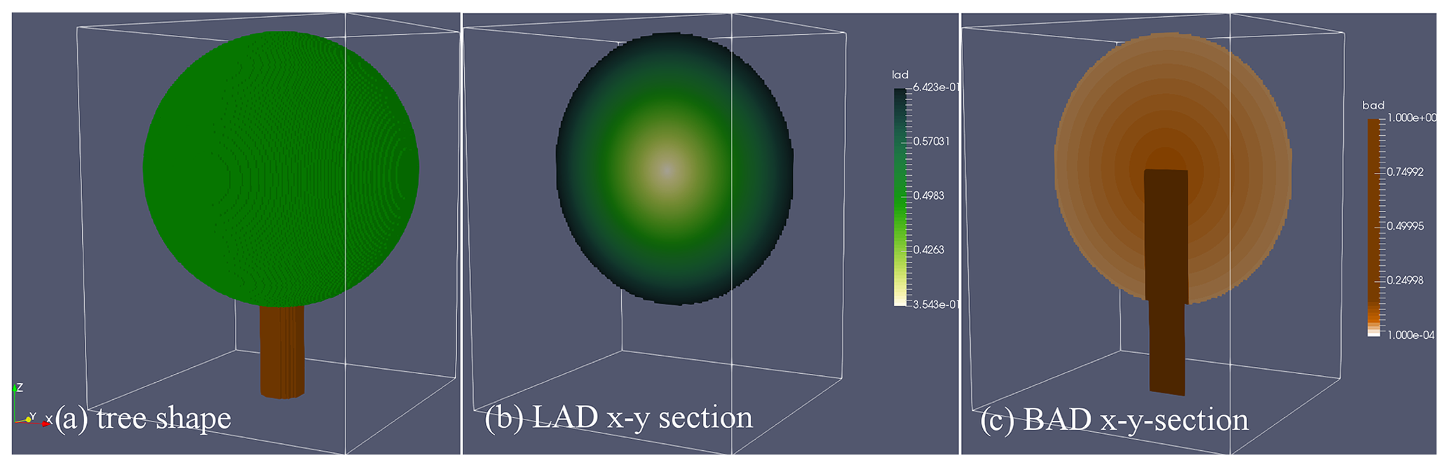
Figure 15 Exemplary distribution of LAD and BAD fields for a spherically shaped tree. Shown are (a) the three-dimensional tree surface and x–y sections of (b) LAD and (c) BAD through the centre of the tree.

5.3.2 Generation of leaf area density fields for tree stands

In many cases, information on individual trees is not available, or tree stands (e.g. forests) have to be represented as a three-dimensional canopy. This is commonly realized by treating each column (y,x) separately and using normalized LAD profiles that are representative of homogeneous canopies. In palm_csd the method of Markkanen et al. (2003) is based on a vertical LAD distribution that is derived from a given LAI field as well as two parameters α and β, which can be varied by the user to represent different types of tree stands. Additionally, a two-dimensional vegetation height field can be prescribed (if available) in order to take into account varying tree heights within the canopy stand. If information on LAI and vegetation height is not available, the user has to provide default values instead. Using this method it is possible to generate idealized vegetation canopies in terms of LAD fields, but it provides no means to derive BAD information. In the future we plan to use a similar method as described in Bohrer et al. (2007) to create BAD fields by synthetically localizing tree trunks.

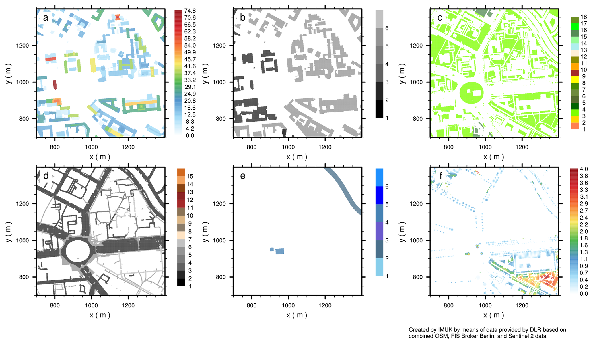
Figure 16 The x–y cross section of static input data for a nested simulation with 1 m grid resolution for a winter scenario for an area around Ernst-Reuter-Platz in Berlin, Germany: (a) building height, (b) building type, (c) vegetation type, (d) pavement type, (e) water type and (f) leaf area index of resolved vegetation (trees). For the sake of illustration (f) displays the leaf area index instead of the leaf area density, with the leaf area index being the vertically integrated leaf area density. Please note in (b)–(e) the label bar contains all possible ∗_type variables as indicated in Table A1, A2, A3 and A5, though only a few types are defined within the displayed area. Panel (b) displays building_type 1 (R1), 2 (R2) and 5 (O2). Panel (c) displays vegetation_type 3 (short grass) and 15 (evergreen shrubs). Panel (d) displays pavement_type 2 (asphalt), 3 (concrete), 4 (sett), 5 (paving stone) and 6 (cobblestone). Panel (e) displays water_type 2 (river) and 4 (pond). Sources: FIS Broker (dl-de/by-2-0: https://www.govdata.de/dl-de/by-2-0, last access: 26 October 2020), Sentinel-2 and OpenStreetMap.

6 Example for a real-world application

To demonstrate the suitability of the input data prepared as described above, the following shows an example static driver and simulation of a part of Berlin. The static driver of this example can be found in the Supplement to this paper.

Figure 16 shows static input data for a nested simulation with 1 m grid resolution. The simulation set-up contains several residential and office buildings with different heights around Ernst-Reuter-Platz, Berlin. The streets indicate different types of pavement, e.g. with asphalt, concrete and cobblestones. Further, grass areas and evergreen shrubs are present within the simulation domain, as well as water ponds and the river Spree. The LAI indicates areas with resolved-scale trees, with single trees planted along pedestrian walks (e.g. in the northwest area of the displayed domain) but also more continuous areas with trees within the Tiergarten park area (see southeast area of the displayed domain).

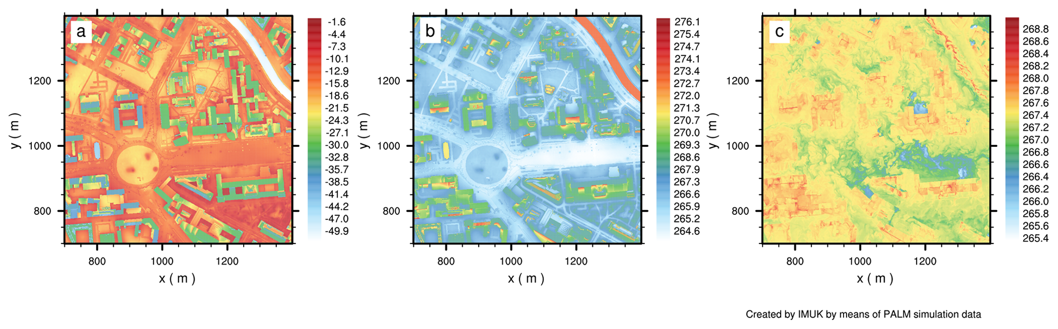
Figure 17 The x–y cross section of (a) surface net radiation (W m⁻²), (b) surface temperature (K) and (c) 2 m potential temperature (K) for a nested simulation with 1 m grid resolution for a winter scenario at 18 January 2017, 00:00 UTC, for an area around Ernst-Reuter-Platz in Berlin, Germany. The displayed area is the same as in Fig. 16.

Figure 17 shows the corresponding horizontal cross sections of surface net radiation, surface temperature, as well as 2 m potential temperature for an area around Ernst-Reuter-Platz in Berlin, Germany. The surface net radiation and surface temperature show a clear dependence on the underlying surface. For example, the building roofs indicate a larger negative surface net radiation but a higher surface temperature compared to other surfaces. Further, pavement surface indicates a only small negative surface net radiation but relatively low surface temperatures. The river and the small ponds show a comparably high surface temperature resulting in a larger negative surface net radiation. The 2 m potential temperature correlates with the underlying surface as well, e.g. with lower values within wide street canyons and larger values in densely built-up areas.

The input data described in this article are also already used in several other studies. A validation of the dynamic core of PALM against wind tunnel data for a city quarter in Hamburg, Germany, is presented by Gronemeier et al. (2020), where the input data of Hamburg as described in this paper were used. A subset of 6000 m by 2880 m around the HafenCity has been selected and rotated anticlockwise by 200^∘ to match the prevailing wind direction. Comparison between the PALM simulation result and the wind tunnel experiment shows mainly similar wind directions but lower wind speeds. As this difference in wind speed decreases at lower spatial resolutions, Gronemeier et al. (2020) assume that this is caused by an overestimated z0 of the building walls in the PALM simulation. The roughness of walls is further increased when building walls are not aligned to the grid and “stair case”-like walls occur. This issue cannot be avoided all together but is minimized when using small grid cells. Furthermore, Gronemeier et al. (2020) emphasized that it is of utmost importance to cautiously check the input data. Especially in large data sets, erroneous or false buildings are hard to spot but can have large influences on the wind pattern, especially if they are located in an upwind part of the study area.

Salim et al. (2020) assessed the importance of radiative transfer processes in urban climate models, in this case PALM6.0. They analysed both a simple urban configuration as well as a real-world configuration of the area around Ernst-Reuter-Platz in Berlin using the same data as used in the example above. They found comparable results regarding the radiative transfer processes for the simple urban area as for the real-world area, although the results for the real-world area were much more heterogeneous, as to be expected.

The sensitivity of the simulation results with respect to variations in the input data is further discussed in Belda et al. (2020) (using a different set of input data). In this study, the sensitivity of air and surface temperature, MRT, PET and PM10 within the PALM6.0 as a response to modification of basic surface material parameters as well as to common urbanistic strategies was evaluated. It was found that for this kind of simulations, the albedo and emissivity as well as thermal conductivity of walls and volumetric heat capacity of the materials play an important role (Belda et al., 2020).

These experiences with the input data indicate that on the one hand the correct identification of urban objects and heights is important but, on the other hand, also the characterization of these objects as currently defined in the building and vegetation parameters at LOD1 and higher.

Furthermore, a thorough validation of PALM in a real urban environment against in situ measurements is presented in Resler et al. (2020). They especially focus on the representation of surface temperatures in PALM at different types of urban surfaces and also emphasize the need for accurate input data to be in agreement with in situ measurements. A dedicated evaluation of the PALM 6.0 model system for the city of Berlin and Stuttgart is currently on its way within the project framework of [UC]² (Scherer et al., 2019).

7 Conclusions

In the previous sections, the input data requirements of PALM are described; it is demonstrated how these data can be prepared and what steps are carried out in palm_csd to set up the static driver to have all input data ready for PALM. PALM comes with a framework that enables microclimate simulations for a real-world urban environment. Different levels of detail can be provided to PALM. If the model is run with interactive building and land surfaces, a minimum of seven spatial parameters is required: soil type, building height, building ID, building type, vegetation type, pavement type and water type. Each of these parameters can optionally be specified in more detail, based on available data. Sections 3 and 4 illustrate that a vast amount of data exists but rarely exactly in the format required by urban microclimate models. An example of this is the building type. The combination of building use and building age yields the PALM building types. However, it needs to be further analysed whether this is the most accurate representation of the energetic properties of the building, as the building age often does not include any information on renovation and modernization of the building, which can have a huge effect on the energetic properties of a building. Selecting and acquiring suitable data sets is a major task that should be weighted against the available resources to preprocess the input data and the desired detail of the PALM simulations. Additionally, the varying quality of different data sources results in different uncertainties of the input parameters. There are uncertainties resulting from the spatial resolution (e.g. the ability to distinguish small objects), but there can also be mapping or labelling errors and omissions. How these uncertainties propagate into the simulation results needs to be investigated in more detail. To support users in the decision of which parameter is worth the effort of acquiring and preparing more detailed information, sensitivity analyses of the input data sets are planned. Also additional evaluation of LOD1 parameters (such as albedo or thermal conductivity) needs to be carried out, as some of them have a large influence on the simulation result. For albedo, it could also be considered to derive such values separately for each grid cell, e.g. using remote sensing. As the preprocessing of the input data is tedious, it is aimed to develop a processing chain that support users in formatting their GIS data (e.g. shapefiles, geoTIFF, WFS) into a NetCDF file following the requirements of PALM. Existing standardized workflows such as those of WUDAPT (Ching et al., 2018) or MApUCE (Bocher et al., 2018) are interesting examples that should be considered further. To support model users in their data acquisition, a database with freely available geospatial data for the mandatory set of parameters of PALM is aimed at. This will provide users a starting point for running PALM simulations. The primarily target will be Germany, but Europe-wide or global data can also be included, insofar the data sources allow this.

Appendix A: Palm input data standard (PIDS) tables

Table A1 Land use classification parameters according to vegetation_type based on the Integrated Forecasting System (IFS) classification. Note that the land use class 13 (ice caps and glaciers) has not been implemented yet. r_c,min is the minimum canopy resistance, LAI is leaf area index, c_veg is vegetation coverage, g_D is a canopy resistance coefficient, z₀ and z_0,h are the roughness lengths for momentum and heat, respectively, Λ_s and Λ_u are the bulk heat conductivities between skin and soil layer for stable and unstable stratification, respectively, f_sw,in is the fraction of absorbed shortwave radiation by the vegetation canopy, and ϵ is the surface emissivity.

Table A2 Building classification parameters according to building_type based on building age and usage.

Table A3 Pavement classification parameters according to pavement_type based on OpenStreetMaps. Thermal conductivity and heat capacity settings of the subsurface pavement layers are given in Table A4. Italic values are preliminary. z₀ and z_0,h are the roughness lengths for momentum and heat, respectively, and ϵ is the surface emissivity.

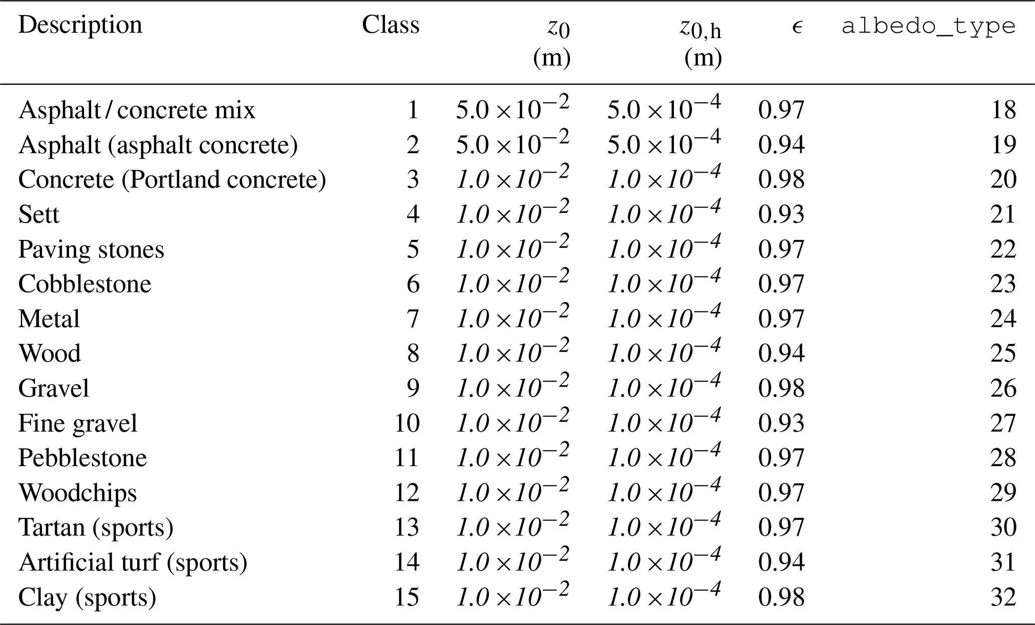
Table A4 Thermal conductivity λ_T,i (in W m⁻¹ K⁻¹) and heat capacity (ρC)_i (in J K⁻¹) of subsurface layer i according to pavement_type classification. The italic values are preliminary. The subscript indicates the respective pavement layer. The pavement layers are defined between depth: 0–0.01, 0.01–0.03, 0.03–0.07, 0.07–0.15, 0.15–0.3 and 0.3–0.5 m.

The layers 1–6 have widths of 0.01, 0.02, 0.04, 0.06, 0.14 and 0.26 m, respectively.

Table A5 Water classification parameters according to water_type. Italic values are preliminary. z₀ and z_0,h are the roughness lengths for momentum and heat, respectively, and ϵ is the surface emissivity.

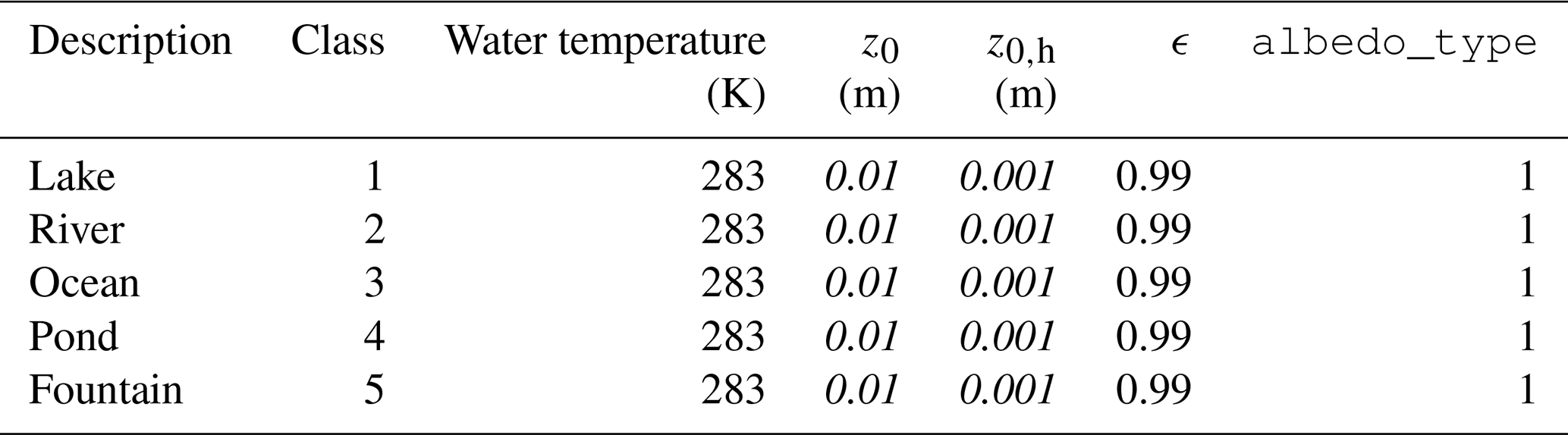
Table A6 Soil classification parameters according to soil_type. α_vG, l_vG and n_vG are van Genuchten parameters, γ_w,sat is the hydraulic conductivity at saturation, and m_sat, m_fc, m_wilt, and m_res are the volumetric soil moisture at saturation, at field capacity, at wilting point, and the residual soil moisture, respectively.

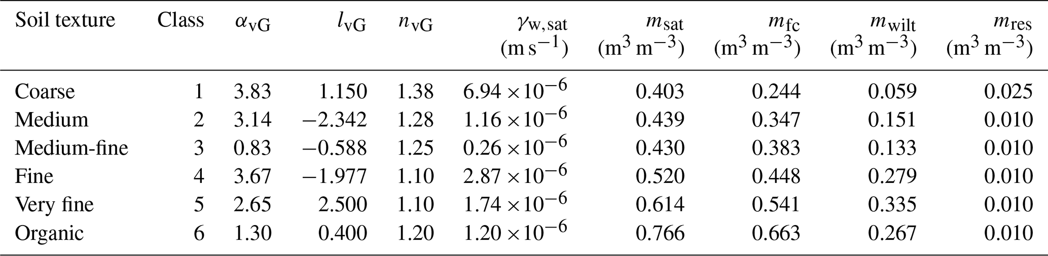
Table A7 Surface albedo classification parameters according to albedo_type. Italic values are preliminary

Appendix B: Lookup tables for various input data sources

Table B1 CLC classes to PALM vegetation type.

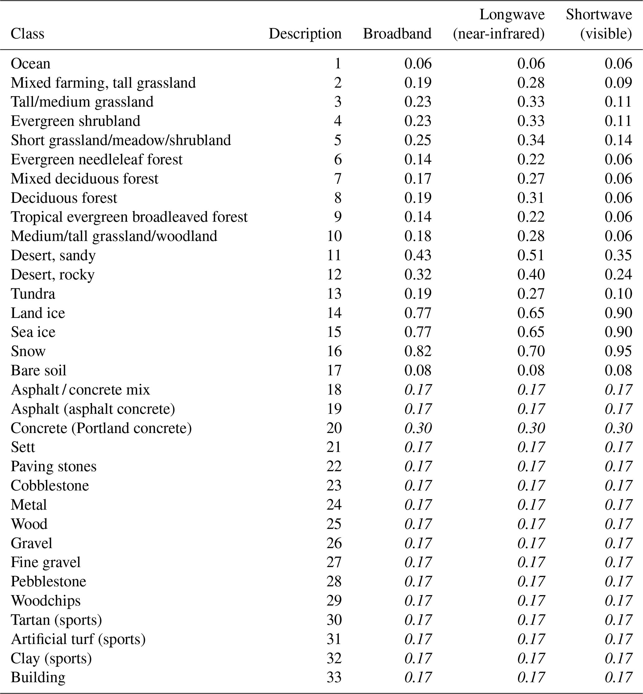
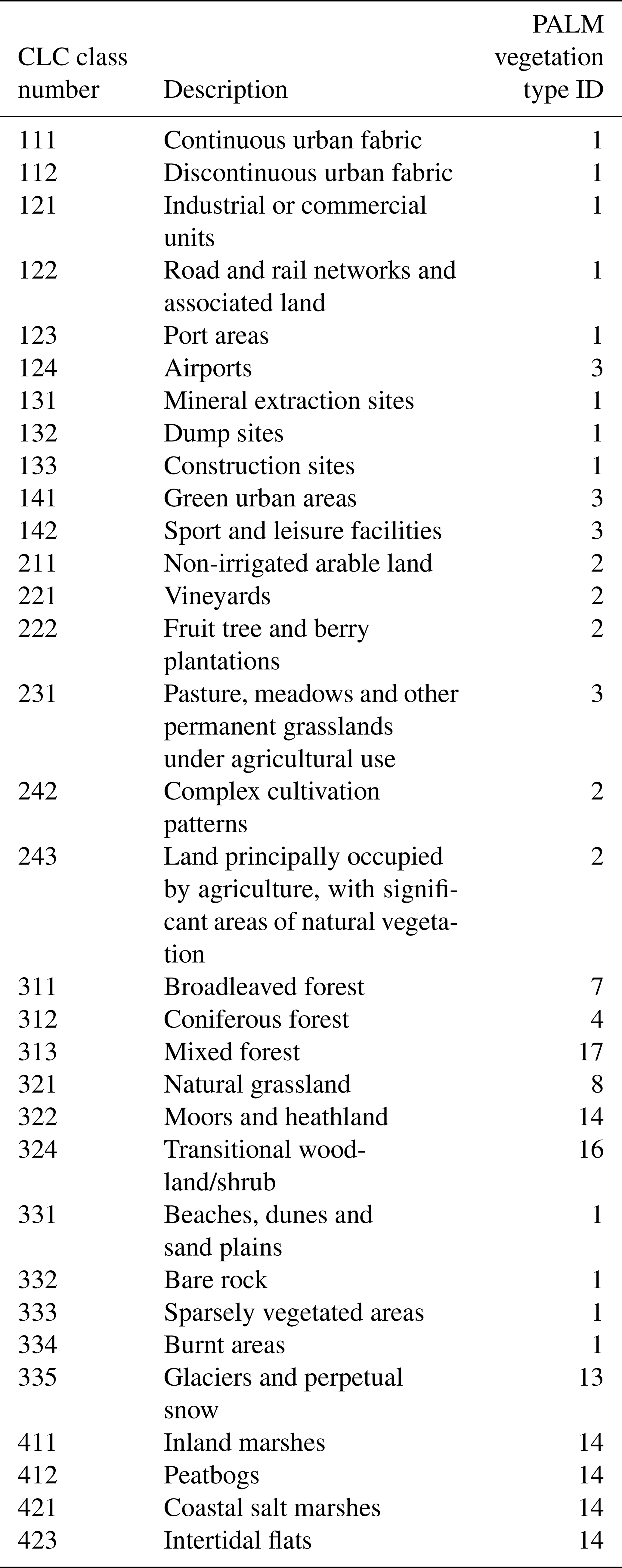
Table B2 OSM land use classes to PALM vegetation type. “255” is a fill value, assigned to non-vegetation pixels.

Table B3 Biotope type groups of the biotope map Hamburg to PALM vegetation type.

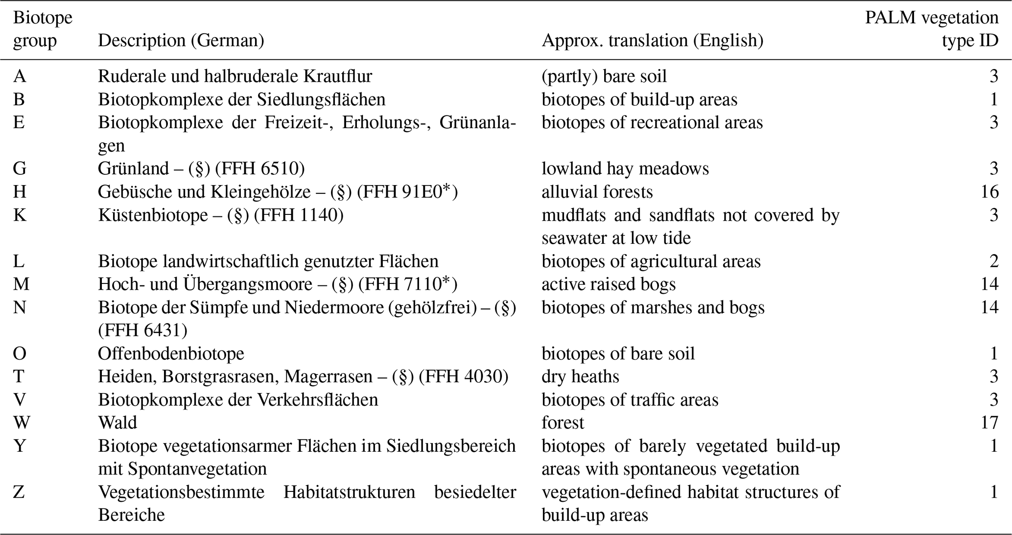
Table B4 OSM pavement labels and according PALM pavement types.

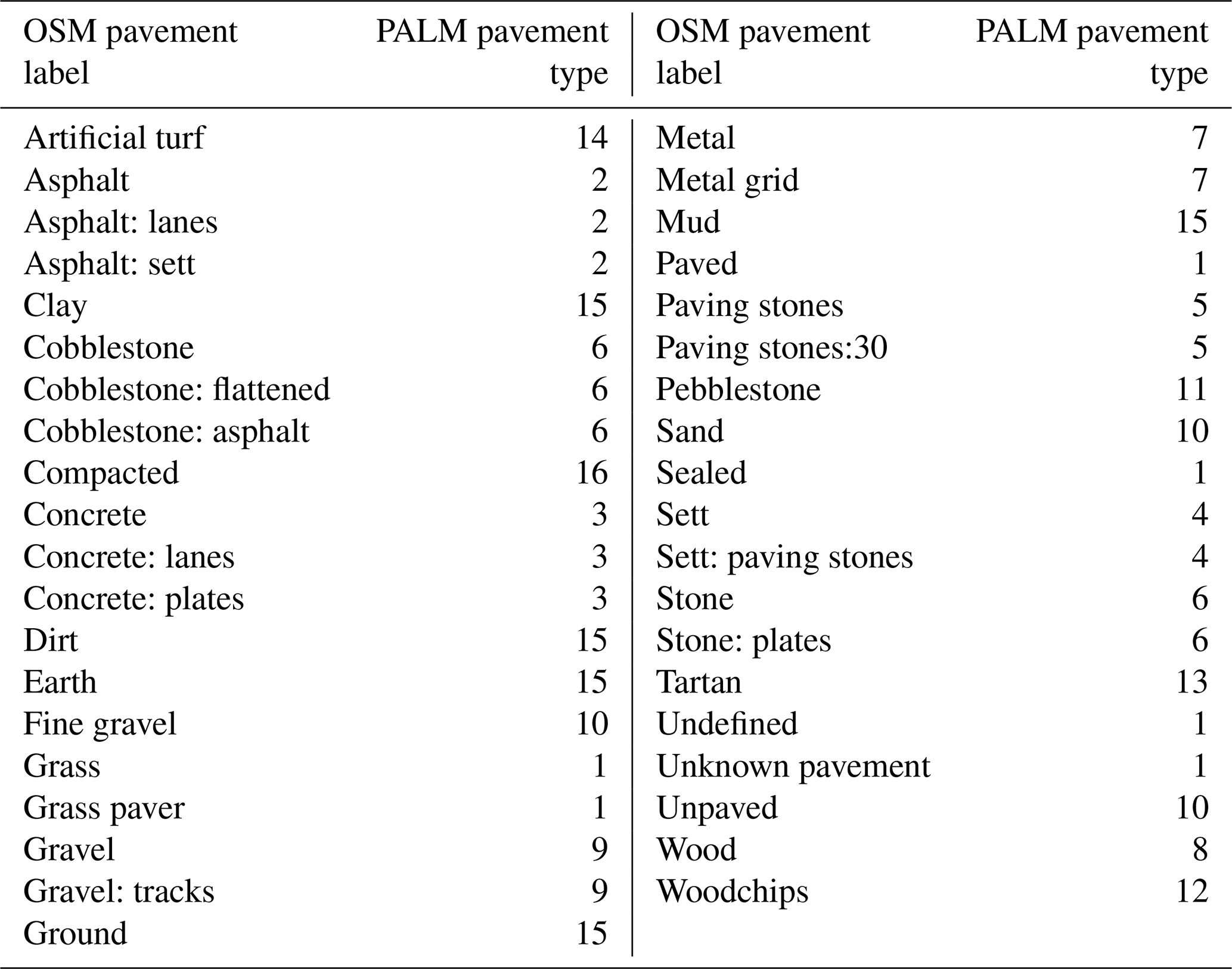
Table B5 OSM road types and corresponding PALM pavement type. The buffer width in this table is only used to convert the line objects into areas if no value is indicated for street width in the OSM data. If the number of lanes is indicated, the street width listed in Table B6 is applied.

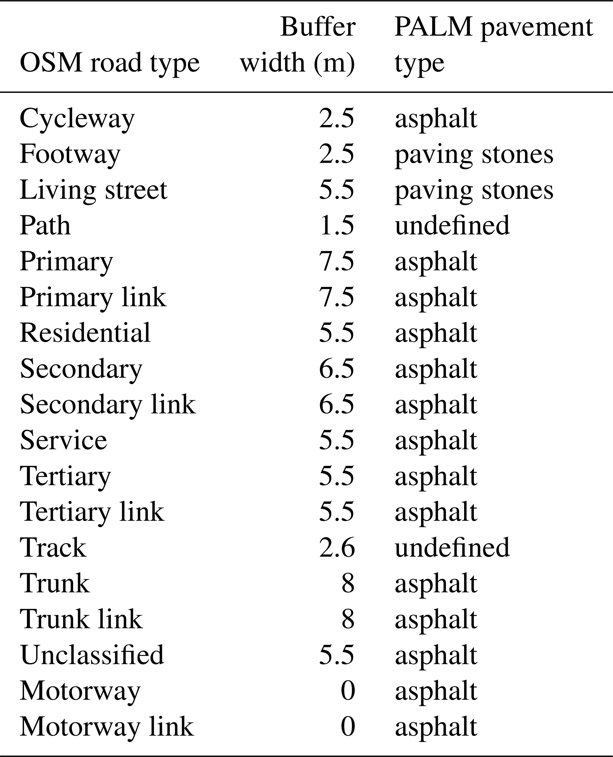
Table B6 Assumed road width when in OSM the number of lanes is indicated.

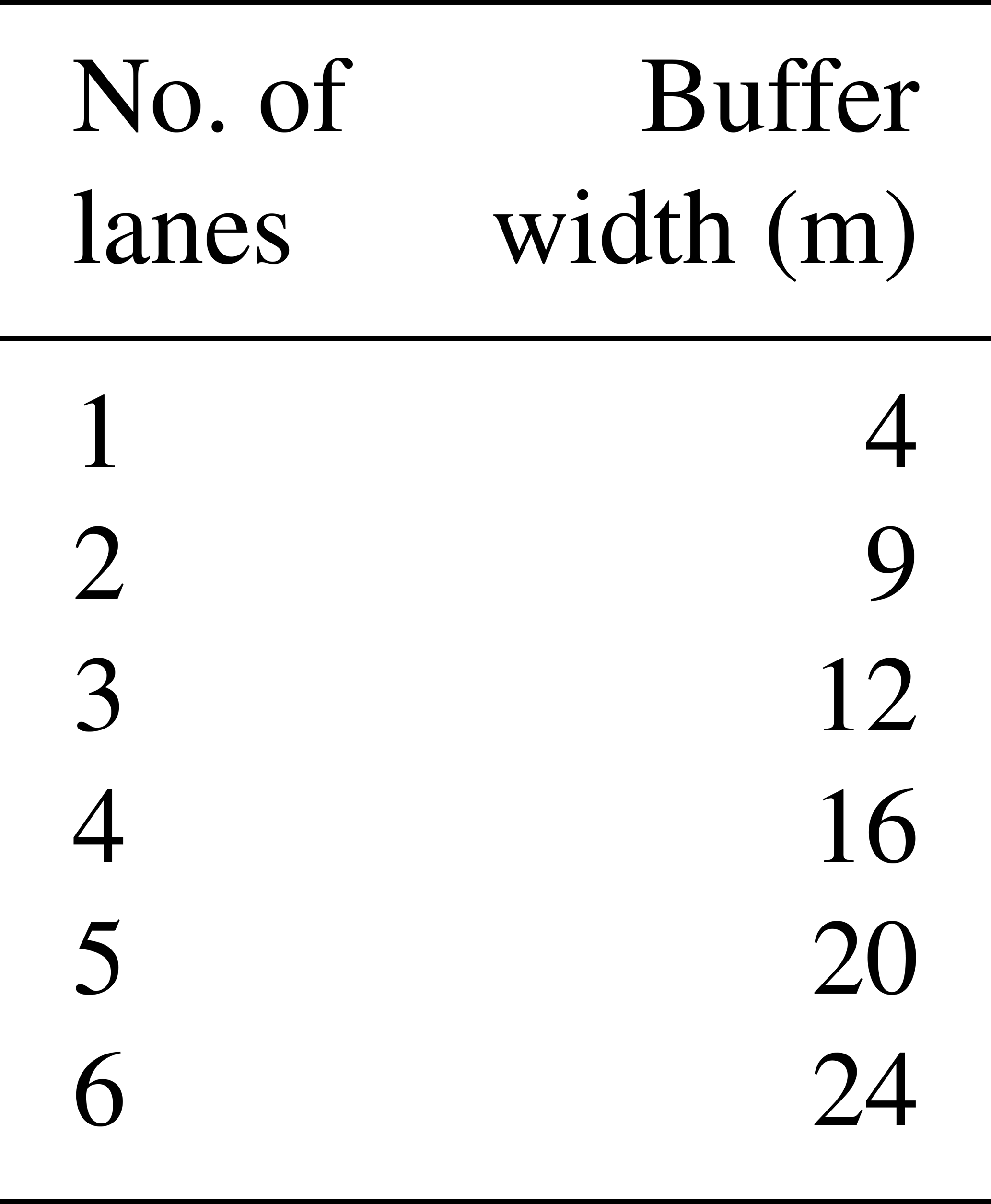
Table B7 Berlin ISU5 (Informationssystem Stadt und Umwelt, English: Information System City and Surroundings) land use descriptions to PALM building type. The building function can be R = residential, O = other, X = no building. The age classes refer to the building period before 1951 (1), between 1951 and 2000 (2), and after 2000 (3). The combination of the function and the building age according to Table A2 results in the PALM building type.

Table B8 ALKIS land use descriptions to PALM building type. The building function can be R = residential, O = other, X = no building. The combination of the function and the building age according to Table A2 results in the PALM building type.

Table B9 OSM values to PALM water type. “255” is a fill value, assigned to non-water pixels.

Table B10 CLC classes to PALM water type.

Table B11 Biotope types of Hamburg to PALM water type.