the Creative Commons Attribution 4.0 License.
the Creative Commons Attribution 4.0 License.
 | 18 Nov 2020
Sensitivity of spatial aerosol particle distributions to the boundary conditions in the PALM model system 6.0
Pontus Roldin
Jani Strömberg
Anna Balling
Sasu Karttunen
Heino Kuuluvainen
Jarkko V. Niemi
Liisa Pirjola
Topi Rönkkö
Hilkka Timonen
Antti Hellsten
High-resolution modelling is needed to understand urban air quality and pollutant dispersion in detail. Recently, the PALM model system 6.0, which is based on large-eddy simulation (LES), was extended with the detailed Sectional Aerosol module for Large Scale Applications (SALSA) v2.0 to enable studying the complex interactions between the turbulent flow field and aerosol dynamic processes. This study represents an extensive evaluation of the modelling system against the horizontal and vertical distributions of aerosol particles measured using a mobile laboratory and a drone in an urban neighbourhood in Helsinki, Finland. Specific emphasis is on the model sensitivity of aerosol particle concentrations, size distributions and chemical compositions to boundary conditions of meteorological variables and aerosol background concentrations. The meteorological boundary conditions are taken from both a numerical weather prediction model and observations, which occasionally differ strongly. Yet, the model shows good agreement with measurements (fractional bias <0.67, normalised mean squared error <6, fraction of the data within a factor of 2 >0.3, normalised mean bias factor <0.25 and normalised mean absolute error factor <0.35) with respect to both horizontal and vertical distribution of aerosol particles, their size distribution and chemical composition. The horizontal distribution is most sensitive to the wind speed and atmospheric stratification, and vertical distribution to the wind direction. The aerosol number size distribution is mainly governed by the flow field along the main street with high traffic rates and in its surroundings by the background concentrations. The results emphasise the importance of correct meteorological and aerosol background boundary conditions, in addition to accurate emission estimates and detailed model physics, in quantitative high-resolution air pollution modelling and future urban LES studies.
- Article
(3474 KB) - Full-text XML
-
Supplement
(3170 KB) - BibTeX
- EndNote


Exposure to outdoor air pollution is a major global threat resulting up to 0.8 million premature deaths in Europe (Lelieveld et al., 2019) and 3 million worldwide (Lelieveld et al., 2015; WHO, 2016) every year. Specifically, aerosol particles can be extremely harmful, and based on a recent study by Burnett et al. (2018) outdoor fine particulate air pollution (PM2.5) solely could have caused up to 8.9 million deaths worldwide in 2015. As over half of the global population lives in cities (55 % according to UN, 2019), urban air quality is of major importance. In addition to high population densities, urban areas are characterised by major air pollutant sources, namely traffic exhaust and road dust, being at the same height where urban dwellers inhale outdoor air. However, the dispersion of these traffic-related pollutants is not straightforward as buildings, trees and other obstacles modify the flow within the urban canopy and hence also pollutant dispersion (Tominaga and Stathopoulos, 2013) as well as the environment for aerosol dynamic processes and chemical reactions to occur.
As a consequence of the complex interactions between the urban morphology, meteorology, local emissions and air pollutant dynamics and chemistry, air quality is highly variable both in time and space, and strong concentration gradients are observed in urban areas. However, measurements from a single monitoring station nearest to the individual's residence, hospital, or primary health care clinic have commonly been applied in air pollution exposure studies (Andersen et al., 2012; Adam et al., 2015), which can lead to notable errors. Moreover, both the size and chemical composition of aerosol particles are of major importance when it comes to their health impacts (Kampa and Castanas, 2008; Kelly and Fussell, 2012). For instance, particle deposition in lungs depends strongly on the inhaled particle size (Hussain et al., 2011), and thus the negative health effects of aerosol particles have been found to correlate more strongly with the surface area of particles than their number or mass (Brown et al., 2001; Oberdörster et al., 2005).
Computational fluid dynamics (CFD) models have been successfully applied in studying the air flow and dispersion of air pollutants in urban areas. Mainly models based on either Reynolds-averaged Navier–Stokes (RANS; e.g. Baik et al., 2009; Kwak et al., 2015; Santiago et al., 2020) or large-eddy simulation (LES; e.g. García-Sánchez et al., 2018; Letzel et al., 2012; Salim et al., 2011) have been utilised. While being computationally more expensive than RANS, LES has been shown to perform better in resolving instantaneous turbulence structures in a complex urban environment (García-Sánchez et al., 2018; Salim et al., 2011). Further, air pollutant concentrations can be significantly modified by their chemical and physical processes (Kurppa et al., 2019; Nikolova et al., 2016; Zhong et al., 2020), especially as the residence time of air pollutants is increased in a complex urban environment (Gronemeier and Sühring, 2019; Ramponi et al., 2015). Therefore, a detailed module describing the characteristics of air pollutants and their dynamics is needed to enable modelling aerosol particles of different size, chemical composition and harmfulness. To date, only a few LES models include a module for treating aerosol particles with a specific size distribution and chemical composition and their dynamic processes (Kurppa et al., 2019; Steffens et al., 2013; Zhong et al., 2020).
The Sectional Aerosol module for Large Scale Applications (SALSA) (Kokkola et al., 2008) was recently implemented to the PALM model system (Kurppa et al., 2019) to consider the impact of aerosol dynamic processes on aerosol concentrations and size distributions and to study the relative importance of pollutant dispersion and aerosol dynamic processes. A model evaluation by Kurppa et al. (2019) in central Cambridge, UK, showed the model to be capable of reproducing the vertical distributions of aerosol size distribution in a simple street canyon. However, due to the lack of observations, the capability of the model to reproduce the horizontal distributions of aerosol particles has not been studied yet. Also the meteorological conditions were limited to a single day and the examined street canyon had no vegetation.
Still, even if the air pollutant processes would be modelled accurately, correct boundary conditions for the meteorological variables and air pollutant concentrations are vital for realistic air quality simulations. Boundary conditions can be drawn from observations, which are however typically point measurements that lack spatial representatives and also are prone to measurement errors. Another alternative is to use model data, which provide a good spatial coverage but not necessarily stable performance in all prevailing weather conditions. Previously, CFD models have been successfully coupled with mesoscale models to study the impact of larger-scale atmospheric features on microscale interactions (e.g. Baik et al., 2009; Heinze et al., 2017; Liu et al., 2012; Michioka et al., 2013; Wyszogrodzki et al., 2012) as well as to consider realistic air pollutant background concentrations (Kwak et al., 2015). Recently, Santiago et al. (2020) investigated the sensitivity of RANS-based urban PM10 (particulate matter with aerodynamic diameter < 10 µm) simulations on the meteorological boundary conditions and showed the model performance to be improved when replacing the wind direction (WD) predicted by the Weather Research and Forecasting (WRF) model with the observed WD. However, Santiago et al. (2020) only modelled passive PM10 without taking into account chemical or physical transformation of aerosol particles. Hence, it is still unclear how much uncertainty in aerosol particle concentrations and size distributions is caused by model boundary conditions.
To further assess the performance of SALSA2.0 in the PALM model system 6.0 in simulating the spatial distribution of aerosol particle concentrations in an urban area and to examine the importance of meteorological and aerosol background boundary conditions, we will use observations made during an extensive measurement campaign in an urban neighbourhood in Helsinki, Finland, in summer and winter 2017. The campaign focused on the spatial variability of aerosol particle number, surface area and mass both in horizontal and vertical as well as aerosol size distributions and chemical composition. The observations were carried out with a high temporal and spatial resolution using a mobile laboratory and a drone. The model is evaluated at three observation periods with different prevailing meteorological conditions.
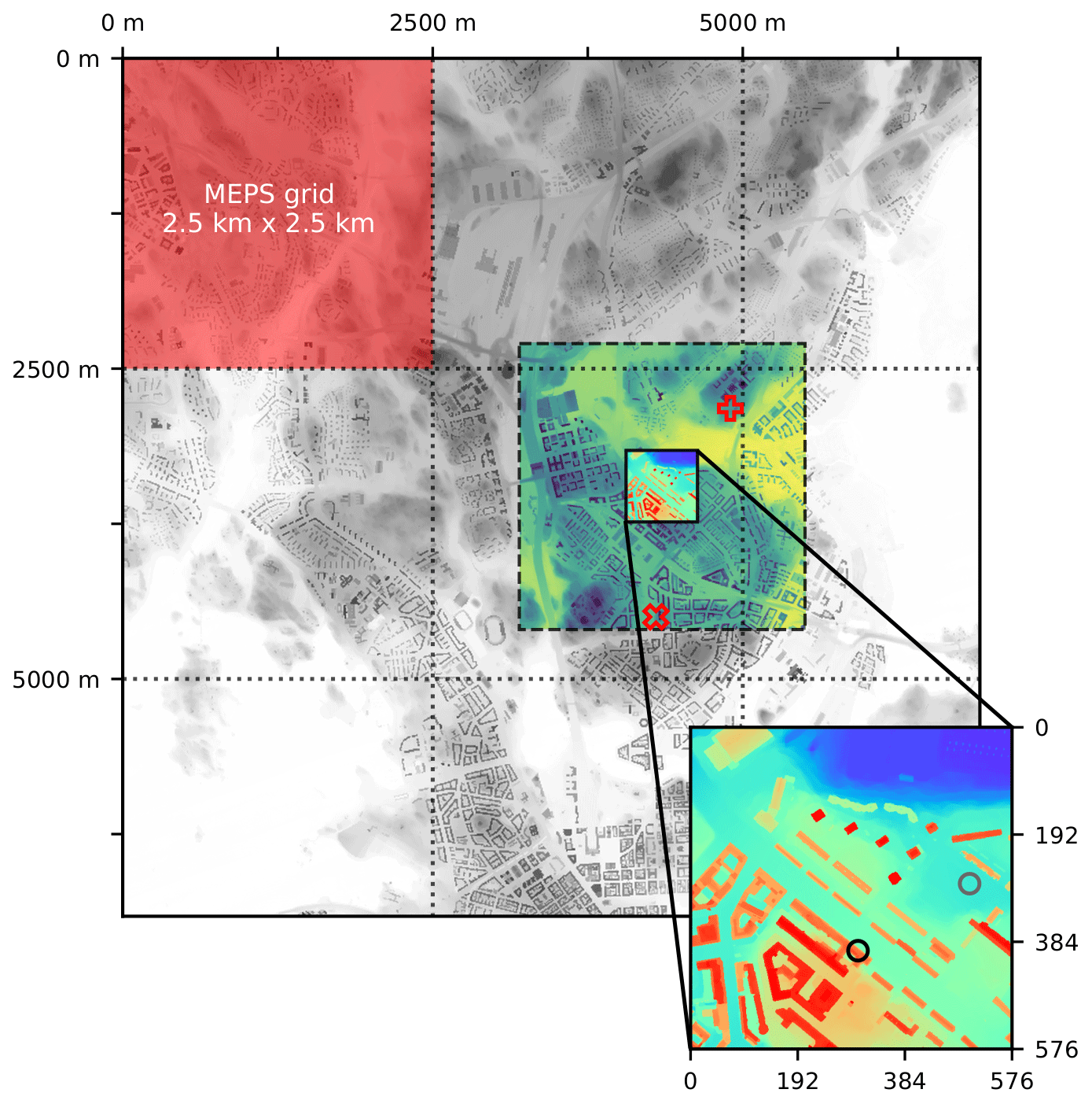
Figure 1The modelling domain: root in grey, parent in viridis (dashed line) and child in rainbow (solid line). The grid size of the MEPS data is illustrated with a red area and dotted lines. The background air quality monitoring sites are marked with an empty red + sign (SMEAR III) and an empty red × sign (Kallio). In the zoomed figure over the child domain, the supersite is marked with a black circle and the background measurement point of the Sniffer mobile laboratory with a grey circle.
2.1 Measurement campaign
The model evaluation and sensitivity study is conducted around an Helsinki Region Environmental Services Authority (HSY) air quality monitoring site, hereafter referred to as the “supersite”, in Helsinki, Finland (60∘11′47′′ N, 24∘57′07′′ E). The site is located 3 km north–northeast from the Helsinki city centre, and it is characterised as an urban street-canyon curbside station with a traffic rate of around 28 000 on a workday, of which 12 % are heavy-duty vehicles (City of Helsinki, 2018b). The street canyon is 42 m wide and the mean building height is around 19 m on the southwestern and 16 m on the northeastern side of the street (see Fig. 1 in Kuuluvainen et al., 2018), resulting in a height-to-width ratio of 0.42. The supersite consists of a container (length 8.0 m, width 1.7 m and height 2.7 m) equipped with standard air quality measurement devices measuring from 4 m above ground level.
To get information about the spatial variability of air pollutants around the supersite, a 2-week measurement campaign was conducted in summer (6–16 June) and winter (28 November–11 December) 2017. During both campaigns, the horizontal distribution of air pollutants in the neighbourhood was monitored on non-rainy days using a mobile laboratory, and additionally during two intensive observation periods the vertical profiles of aerosol particles were measured using a drone.
Table 1Instrumentation of the Sniffer mobile laboratory. Abbreviations: PSD is the aerosol particle number size distribution, Ntot is the total aerosol particle number concentration, and PM1 is the mass of particulate matter with aerodynamic diameter < 1 µm.
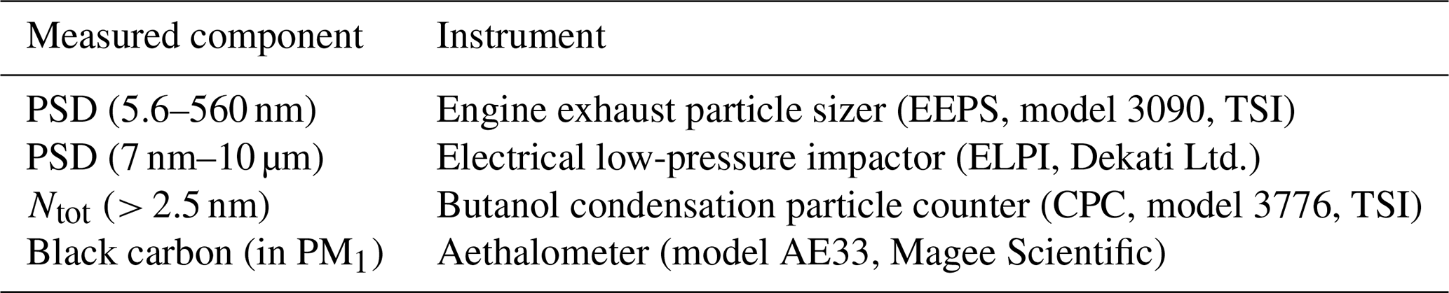
The Sniffer mobile laboratory (Pirjola et al., 2004) measured the horizontal distribution of trace gases and aerosol particle concentrations and size distribution. The measurements were done in 1–2 h slots with a 1 s temporal resolution during the morning and afternoon rush hours, around noon and in the late evening. During each observation period, the Sniffer was driving along a main street (Mäkelänkatu) and a side street as well as standing at the supersite, opposite the supersite and on a field 185 m from the main street (hereafter the “background”). The instrumentation of the Sniffer is given in Table 1 and the measurement locations in Fig. S1 in the Supplement. The main inlet was situated above the windshield at 2.4 m and a global positioning system (model GPS V, Garmin) recorded the van speed and position. For a detailed description of the Sniffer, see Enroth et al. (2016); Pirjola et al. (2016).
During the intensive observation periods, a multi-rotor drone (X8, VideoDrone Finland Ltd.) carried an electrical particle sensor (Partector, Naneos GmbH) to measure the vertical distribution of the alveolar lung-deposited surface area (LDSA) of aerosol particles, which describes the total aerosol surface area penetrating the deepest parts of the lungs (see, e.g. Kuula et al., 2020, and references within). The measurement were done on both sides of the street canyon when the Sniffer was simultaneously driving. The drone was flown 10 times up and down between z=2 and 50 m during one 30 min measurement interval, after which measurements were repeated on the other side. Each intensive observation period started by measuring LDSA at the supersite and ended on the other side. Measurements were started at 3 m from the building wall and the horizontal location was kept constant with a GPS sensor of the drone. Additionally, LDSA was measured at the supersite by a Pegasor AQ Urban sensor (Pegasor Ltd.) and on the other side by a DiSCmini (Testo Ltd.) or with another Partector at 1 m and in winter also at 14 m. For the details of the instrumentation, see Kuuluvainen et al. (2018).
The sensitivity of the results to the PALM model boundary conditions is examined during the following three periods: the morning (07:16–09:15 LT) and evening (20:26–21:14 LT) of 9 June, and the morning (07:20–09:14 LT) of 12 December.
2.2 Additional measurements
In addition to the Sniffer and drone measurements, we use stationary aerosol observations from the supersite and two urban background monitoring sites: Kallio site operated by HSY and SMEAR III (Station for Measuring Ecosystem Atmospheric relations; Järvi et al., 2009) around 1.0 km southwest and 0.8 km northeast from the supersite, respectively (Fig. 1). See Table S1 for the instrumentation. In addition to aerosol observations, meteorological data (wind speed, wind direction, air temperature) from the SMEAR III measurement tower (z=31 m) and Kivenlahti meteorological measurement mast 17.4 km west from the supersite (Wood et al., 2013) are used in the study.
3.1 Model description
This study applies the PALM model system, version 6.0 (revision 4416) (Maronga et al., 2015, 2020), which features an LES core for atmospheric and oceanic boundary layer flows. PALM solves the non-hydrostatic, filtered, incompressible Navier–Stokes equations of wind (u, v and w) and scalar variables (subgrid-scale turbulent kinetic energy e, potential temperature θ and specific humidity q) in Boussinesq-approximated form. PALM is especially suitable for complex urban areas, due to its features such as a Cartesian topography scheme and a plant canopy module, which are applied here to include the aerodynamic impact of both solid buildings and permeable vegetation on the flow. Furthermore, the so-called PALM-4U (short for PALM for urban applications) components have recently been implemented in PALM (Maronga et al., 2020), including the SALSA aerosol module, the online chemistry module and the self-nesting and offline nesting features, which are all applied in this study.
SALSA (Kokkola et al., 2008; Kurppa et al., 2019) describes an aerosol size distribution by a number of size bins (10 by default), and each bin can be composed of different chemical components. Chemical components included are sulfuric acid (H2SO4), organic carbon (OC), black carbon (BC), nitric acid (HNO3), ammonia (NH3), sea salt, dust and water (H2O). SALSA contains the following aerosol dynamic processes: coagulation, nucleation, dry deposition on solid surfaces and resolved-scale vegetation, and condensation and dissolutional growth by gaseous H2SO4, HNO3, NH3 and semi- and non-volatile organics (SVOC and NVOC). The gaseous compounds can be transferred to SALSA from the online chemistry module, which is based on the Kinetic Pre-Processor (KPP; Damian et al., 2002) version 2.2.3 and an adapted version of the KP4 pre-processing tool (Jöckel et al., 2010). The implementation is flexible, allowing the user to choose the chemical mechanism and components being considered. In this study, a simplified mechanism describing photochemical smog is applied (see Sect. S3.2 in the Supplement). Photolysis is parameterised based on Saunders et al. (2003). However, the transfer of different organic vapours from the chemistry module to SALSA is still under development.
To capture the dominant turbulent eddies of the atmospheric boundary layer (ABL) in LES, the horizontal extent of the modelling domain should span over several ABL heights; see, e.g. Fishpool et al., 2009; Chung and McKeon, 2010; Auvinen et al., 2020. At the same time, to resolve most of the kinetic energy within street canyons, a high enough grid resolution (on the order of ∼ 1 m) is needed (Xie and Castro, 2006). Furthermore, uncertainty arising from the lateral boundary conditions usually decreases with increasing horizontal dimensions. To fulfill these contradicting requirements, a self-nesting feature has been included in PALM (Hellsten et al., 2017; Maronga et al., 2020). In self-nesting, one or several child domains are nested within a parent domain and the child obtains its boundary conditions from its parent. Furthermore, PALM incorporates an automated mesoscale offline nesting with a mesoscale operational weather prediction model, which allows realistic, non-cyclic and non-stationary boundary conditions for the flow. As the mesoscale data do not contain resolved-scale turbulence, turbulence must first be developed within the PALM domain. To reduce the time and distance for the mesoscale flow field to adjust and turbulence to develop within the LES modelling domain, a synthetic turbulence generator within PALM can be applied.
Table 2Dimensions (L), number of grid points (N) and grid resolutions (Δ) of the model domains in the x, y and z directions.

* Δz is stretched with a factor of 1.03 above z=300 m, resulting in a total domain height of 606 m.
Table 3Unit emission factors for traffic combustion (s is solid and g is gaseous) on 9 June between 07:00 and 08:00 LT in units of 10−5 . Abbreviations: PM is the total mass of particulate matter, BC is black carbon, OC is organic carbon, NO is nitrous oxide, NO2 is nitrous dioxide, SVOC is semi-volatile organic carbon, RH is alkanes, H2SO4 is sulfuric acid, N2O is nitrous oxide, and NH3 is ammonia.

3.2 Model domain and morphological data
The model simulations are conducted over a root domain of 6.9 km × 6.9 km, within which two smaller domains, parent and child, are nested progressively (Fig. 1). The dimensions (Lx, Ly, Lz), number of grid points (Nx, Ny, Nz) and grid resolutions (Δx, Δy, Δz) of each domain are given in Table 2. In this study, the focus is on the child domain which matches with the area of the spatial aerosol measurements around the supersite.
Information on the building and vegetation height and land surface elevation are taken from high-resolution raster maps for Helsinki (Auvinen and Aarnio, 2019). The manipulation of the domain input files is done using the Python library P4UL (Auvinen and Karttunen, 2019). Only vegetation higher than m is included in the simulations. Due to the lack of observational data on the leaf area density (LAD) of vegetation, a constant LAD value is applied for all tree crowns above zv,min. In summer, LAD=1.2 m2 m−3 for broadleaf trees (Abhijith et al., 2017), while in winter LAD is decreased to 20 % of the summertime value.
3.3 Meteorological boundary conditions
We apply both modelled and observed data as meteorological boundary conditions, which are set dynamic; i.e. they change with time.
As modelled data, numerical weather prediction data from MetCoOp Ensemble Prediction System (MEPS; Bengtsson et al., 2017; Müller et al., 2017) are applied. MEPS data were downloaded from the data archive (Norwegian Meteorological Institute, 2019b) using the File Interpolation, Manipulation and EXtraction (Fimex) library (Norwegian Meteorological Institute, 2019a). MEPS has a horizontal resolution of 2.5 km (see Fig. 1), 65 vertical levels and 10 ensemble members. It ran four times daily with a 3-hourly cycling for data assimilation (3D-Var). The lateral boundary data are from the European Centre for Medium-Range Forecasts (ECMWF) high-resolution (HRES) atmospheric model. In this study, the MEPS control run, i.e. ensemble member 0 with unperturbed initial and lateral boundary conditions, is used.
Data from the Kivenlahti mast are downloaded from Finnish Meteorological Institute (FMI) Open Data service (Finnish Meteorological Institute, 2020) as 10 min averaged data. On the mast, meteorological observations are conducted at three to eight measurement levels between m. Despite being located 17.4 km from the supersite, the closest observations of the vertical profile of basic meteorological variables are conducted at Kivenlahti. Meteorological observations from the SMEAR III station at z=31 m are downloaded using the SmartSMEAR tool (Junninen et al., 2009).
The initial conditions and dynamic meteorological boundary data are provided to PALM in a so-called dynamic driver. Of the MEPS data, the dynamic driver was created by the following procedure. First, the sigma coordinates were translated to pressure coordinates and further to height coordinates applying the hypsometric equation. Then, u, v, w, θ and water vapour mixing ratio qv were interpolated from the MEPS grid to the PALM grid: first in horizontal over a two-dimensional grid using the cubic spline method and then in vertical using the linear interpolation. The Kivenlahti mast observations, instead, were linearly interpolated in the vertical to the highest observation level, after which a constant value was used. When applying the SMEAR III data, constant values are used for the entire vertical profile. The dynamic driver created from the observational data does not include any horizontal variation.
A mesoscale interface, INIFOR, has been developed to transform mesoscale modelling data into PALM-readable boundary data. However, it is currently only available for COSMO-DE/D2 datasets, which do not cover Finland.
3.4 Air pollutant background concentrations
Similar to the meteorological boundary conditions (Sect. 3.3), both modelled and observed air quality data are used as background concentrations in the simulations. As in the previous model evaluation study (Kurppa et al., 2019), the modelled background aerosol particle number and trace gas concentrations are produced with the trajectory model for Aerosol Dynamics, gas and particle phase CHEMistry and radiative transfer (ADCHEM; Roldin et al., 2011b, a, 2019). ADCHEM is operated as a one-dimensional column trajectory model along the Hybrid Single-Particle Lagrangian Integrated Trajectory (HYSPLIT) (Stein et al., 2015) air mass trajectories, starting 7 d backwards in time (see Figs. S2 and S3 in the Supplement). The gas and aerosol particle compositions and size distributions are simulated along the back trajectories arriving to the coordinates of the supersite. For the emission inventories and parameterisations applied, see Sect. S3.4 in the Supplement. Detailed descriptions of the aerosol and cloud microphysics, new particle formation and gas-phase chemistry mechanisms in ADCHEM are provided by Roldin et al. (2019) and references therein.
To investigate the impact of the background aerosol size distribution (PSD) and concentration on the model simulations, PSD measurements from SMEAR III (see Sect. 2) are applied as an alternative for the modelled values. For simplicity, ADCHEM data are always used for the chemical composition of aerosol particles and gaseous concentrations.
For each PALM simulation, the concentrations are averaged over the simulation time and these temporally constant vertical profiles are then introduced to the simulation domain by a decycling method, in which background concentrations are fixed at the lateral boundaries.
3.5 Air pollutant emissions
In this study, air pollutant emissions only from traffic combustion are included, as traffic is the main pollutant source within the modelling domain (Helsinki Region Environmental Services Authority, 2020). Traffic-lane maps separating different road categories, i.e. main streets, collector roads and residential streets, have been generated by combining lane and street type information from the Map Service (City of Helsinki, 2018a). The lane width is 3.5 m. Emissions are introduced as dynamic surface fluxes.
Aerosol particle emission inventories are typically provided as total mass emission factors EFPM. In SALSA, these would need to be translated to number emission factors EFN, assuming some size distribution for the emitted aerosol particles. However, converting aerosol mass to number is highly sensitive to the assumed size distribution. Therefore, in this study, we choose to apply a number emission factor based on fuel consumption and a number size distribution estimated by Hietikko et al. (2018) at the supersite in May 2017 (see Fig. S4 in the Supplement).
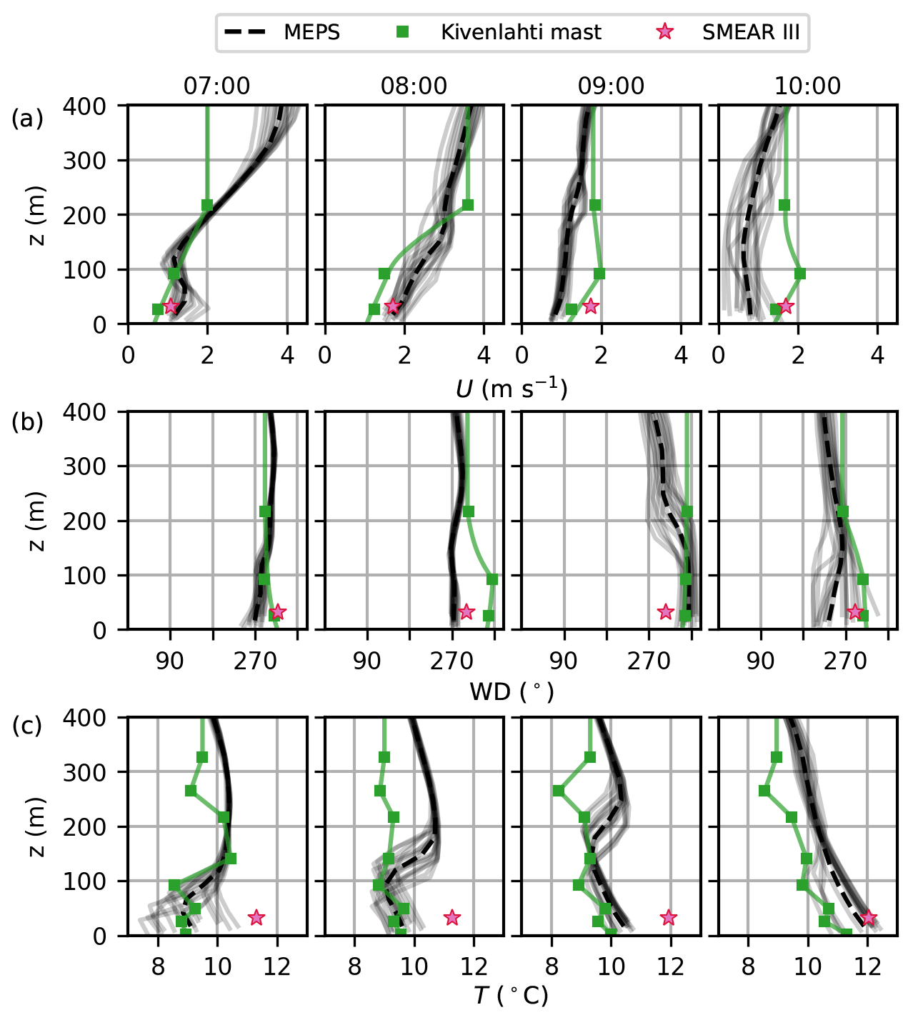
Figure 2Horizontal (a) wind speed U (m s−1), (b) WD (∘) and (c) air temperature T (∘C) on 9 June at local time (UTC+3). The modelled profiles at each MEPS grid point are shown by solid grey lines and their mean by a dashed black line. The observations from the Kivenlahti mast are shown by solid green squares and the interpolated profiles used as boundary conditions by a solid green line. Stars show the SMEAR III observations.
For gaseous compounds, mass composition of aerosol particles and fuel, unit emission factors EF[compound] (Table 3) are calculated using emission inventory by the European Environmental Agency for 2017 (Ntziachristos et al., 2016) and specifically the tier 3 method, which applies information on the mileage per vehicle category and technology, and driving speed. However, since no information on the cumulative mileage for different Euro classes was available, and are based on the tier 1 method (see Ntziachristos et al., 2016, Eq. 28). Furthermore, the following estimates were applied: EFSVOC(g)=0.01EFNMOG (Zhao et al., 2017, Fig. 2), EFRH(g)=0.4EFNMOG (Huang et al., 2015, Fig. 4), where NMOG stands for non-methane organic gas and RH(g) for alkanes, and (Arnold et al., 2006, 2012; Miyakawa et al., 2007). Emitted aerosol particles smaller than 15 nm in diameter are assumed to be composed of 75 % OC and 25 % H2SO4, whereas larger particles contain 72 % BC, 21 % OC and 7 % H2SO4 as estimated from EFPM, EFBC and EFOC.
The hourly vehicle fleet compositions for the neighbourhood are obtained from the Helsinki Region Environmental Services Authority (HSY and Urban Environment Division of the City of Helsinki, personal communication, 1 October 2018), the mileage for each vehicle technology from the ALIISA model (VTT, 2018) and the fuel sulfur content from the LIPASTO database (VTT, 2017). The traffic rates in the neighbourhood are estimated by normalising the mean traffic volumes per each street (Urban Environment Division of the City of Helsinki, Helsinki Region Environmental Services Authority and Helsinki Region Municipalities, 2018) with traffic counts from an online traffic-monitoring station located in the northwestern corner of the child domain (City of Helsinki, personal communication, 3 March 2018). Traffic volumes for both southward and northward traffic are measured separately.
3.6 Model setup
The length of the morning simulations on 9 June and 12 December is 2 h, and only 1 h for the evening simulation on 9 June. Simulation times correspond to the observation periods.
Table 4Simulation abbreviations. WD is the wind direction and PSD is the aerosol particle number size distribution.

For all simulation times, two simulations using either modelled (M) or observed (O) boundary conditions for the flow and background aerosol particle number size distribution (PSD) are conducted. The first setup, hereafter MMETMPSD, applies the modelled meteorological (MET) boundary conditions from the MEPS data and the modelled PSD from the ADCHEM model. The second setup, hereafter , applies the observed meteorological data from the Kivenlahti mast and the observed PSD from SMEAR III. Furthermore, two types of sensitivity tests are conducted for the summer morning. Firstly, model sensitivity on the background PSD is studied by running a simulation with the modelled meteorological boundary conditions and observed background PSD (MMETOPSD). Secondly, the influence of WD on pollutant dispersion is investigated by replacing WD in the MEPS data by WD measured on the Kivenlahti mast (OWD,mastOPSD) or at the SMEAR III station (OWD,SMEAROPSD). As WDSMEAR III is only measured at z=31 m, the wind direction at the model boundaries in OWD,SMEAROPSD is set constant with height. In total, nine different simulations have been conducted.
The aerosol and chemistry modules are run only within the child domain to limit computational costs. In all simulations, the aerosol processes of condensation and dissolutional growth, coagulation, dry deposition and sedimentation are included and calculated every 1.0 s. The aerosol particle size distribution is described by 10 size bins, of which three are within the first subrange (2.5–15 nm) and seven within the second subrange (15 nm–1 µm). Aerosol particles are assumed to be internally mixed and hygroscopic, and can contain H2SO4, OC, BC, HNO3 and/or NH3. The chemical reactions are calculated at every time step of the PALM model.
The advection of both momentum variables and scalars is based on the fifth-order advection scheme by Wicker and Skamarock (2002) together with a third-order Runge–Kutta time-stepping scheme (Williamson, 1980). The pressure term in the prognostic equations for momentum is calculated using the iterative multigrid scheme (Hackbusch, 1985). The roughness height is z0=0.05 m (Letzel et al., 2012) and the drag coefficient applied for the trees is CD=0.3.
Simulations were first run only for the root domain for 1 h, called the precursor run here, after which the final simulations were started. The final simulations including also the nested parent and child domains were initialised using the final state of the precursor run. Offline nesting is used as forcing for the root domain and the parent and child are nested within using one-way self nesting. As SALSA and chemistry are run only within the child domain, for them the nesting is not applied and the boundary conditions of air pollutants are set at the child boundaries. The data output was collected starting after the first 15 min of the final simulation. Simulations were performed on the Centre for Scientific Computing (CSC) Puhti supercluster. Using in total 394 Intel Xeon processor cores, each simulation required 39–80 h of computing time.
The summer morning of 9 June is characterised by very calm northerly–northwesterly winds with the horizontal wind speed at z=30 m and mainly within the lowest 200 m on the Kivenlahti mast (Fig. 2a–b). The MEPS data show more westerly winds, with compared to the Kivenlahti observations, except at 09:00 LT when the modelled and observed WDs agree. Furthermore, the observed U values are up to 0.5 m s−1 lower within the lowest 100 m during the first 2 h and up to 1.0 m s−1 higher during the last 2 h when compared to the MEPS data. As the highest measurement level for U on the Kivenlahti mast is z=217 m, the interpolated profile used as the boundary condition in OMETOPSD underestimates U above 217 m at 07:00 LT. The observed and modelled profiles of air (T) and dew-point temperature (TD) correspond qualitatively well (Figs. 2c and S5 in the Supplement), but the observations show lower (higher) values of T (TD) than MEPS above z=200 m, especially at 08:00–09:00 LT. MEPS also predicts a stronger and shallower surface temperature inversion, which would lead to weaker vertical mixing. Observations at SMEAR III generally follow those on the Kivenlahti mast, except that T is roughly 2 ∘C higher at SMEAR III compared to the Kivenlahti mast and WD typically falls between the MEPS data and Kivenlahti observations. The difference in WD can be explained by flow distortion at SMEAR III due to the adjacent buildings to the north of the measurement site (Nordbo et al., 2012). The observed background aerosol particle number concentrations at SMEAR III are around 80 % lower, and the modelled PSD shows a smaller peak diameter of D=40 nm instead of D=50 nm in the SMEAR III observations (Fig. S6). Furthermore, the observations show a secondary peak at D=14 nm, which is not captured by ADCHEM.
By the evening, the observed U on the Kivenlahti mast had increased to 2.0–2.5 m s−1 at z=30 m (Fig. S7a) and the wind turned to the southwest (Fig. S7b). The modelled and observed WD agree well (), whereas clear discrepancy is shown for U. The MEPS predicts a low-level jet with the maximum U at z=100 m and shows up to 3 m s−1 higher values compared to the Kivenlahti observations at 08:00–09:00 LT. This low-level jet results in a strong wind shear and mechanical turbulence production. Instead, above, U is overestimated in the interpolated Kivenlahti data at 21:00–22:00 LT. The profiles of TD agree relatively well (Fig. S8), whereas MEPS predicts clearly lower T, with a difference up to close to the ground (Fig. S7c). The SMEAR III observations agree with those from the Kivenlahti mast. The modelled and observed background PSD agree in shape, but the peak is observed at D=70 nm compared to D=87 nm in ADCHEM and observed total number concentration is around 35 % lower (Fig. S9).
During the winter morning of 7 December, easterly flow was observed and the wind was turning to southeast with both height and time (Fig. S10a–b). Winds were stronger than in the summer morning, around 2 m s−1 at z=30 m. The observed and modelled WD agree, but MEPS predicts up to 3 m s−1 lower U above the canopy. An inversion layer above the ground is captured both in MEPS and observations (Fig. S10c), yet it is stronger in the observations especially during the first hours. In contrast to T, MEPS predicts down to lower TD compared to the Kivenlahti observations at 09:00 LT (Fig. S11). Similar to the summer morning, the observations on the Kivenlahti mast and SMEAR III are in agreement. Both the modelled and observed PSDs peak at D=30 nm, but the observed total number concentrations is around 60 % higher (Fig. S12).
The model is evaluated against observations at the three different observations periods, and in both summer and winter mornings the evaluation is done separately for both modelling hours.
Table 5The performance measures and acceptance criteria applied in the evaluation: fractional bias (FB), normalised mean squared error (NMSE), factor of 2 (FAC2), normalised mean bias factor (NMBF) and normalised mean absolute error factor (NMAEF). For more details on the acceptance criteria, see Hanna and Chang (2012) and Yu et al. (2006).
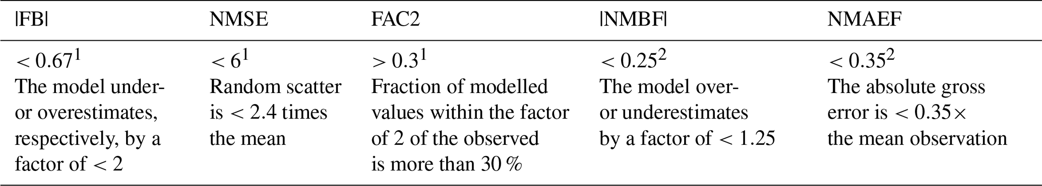
1 Hanna and Chang (2012). 2 Yu et al. (2006).
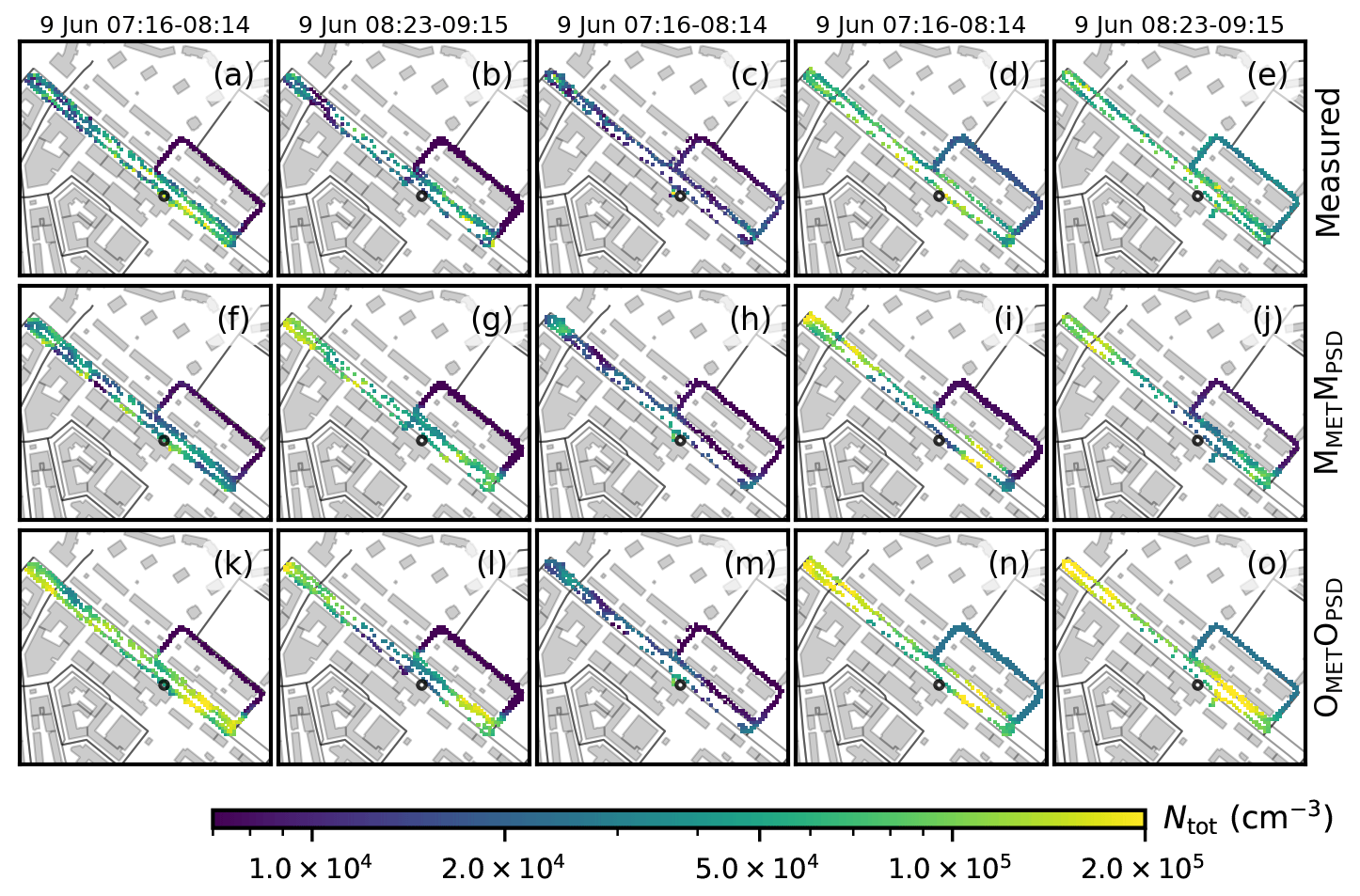
Figure 3Measured (a–e) and modelled (f–o) median total aerosol number concentration (Ntot) along the Sniffer route for the summer morning (a, f, k for the first and b, g, l for the second hour), summer evening (c, h, m) and winter morning (d, i, n for the first and e, j, o for the second hour). The second row shows MMETMPSD and the third OMETOPSD. Measurements are from z=2.4 m and modelled values from z=2.5 m. The supersite is marked with a black circle.
5.1 Performance measures
The following performance measures are applied in the evaluation: fractional bias (FB), normalised mean squared error (NMSE), factor of 2 (FAC2) (Chang and Hanna, 2004), normalised mean bias factor (NMBF) and normalised mean absolute error factor (NMAEF) (Yu et al., 2006). See Table 5 for the acceptance criteria and Appendix A for the equations. In short, FB and NMBF measure systematic error (i.e. bias), NMSE and NMAEF both systematic and random errors, and FAC2 the correct concentration scales. Additionally, the statistical significance of the model error (i.e. the absolute difference between the observations and modelled values) is estimated with a Student's t test for the horizontal distributions of Ntot.
5.2 Horizontal distribution of total aerosol particle number concentration
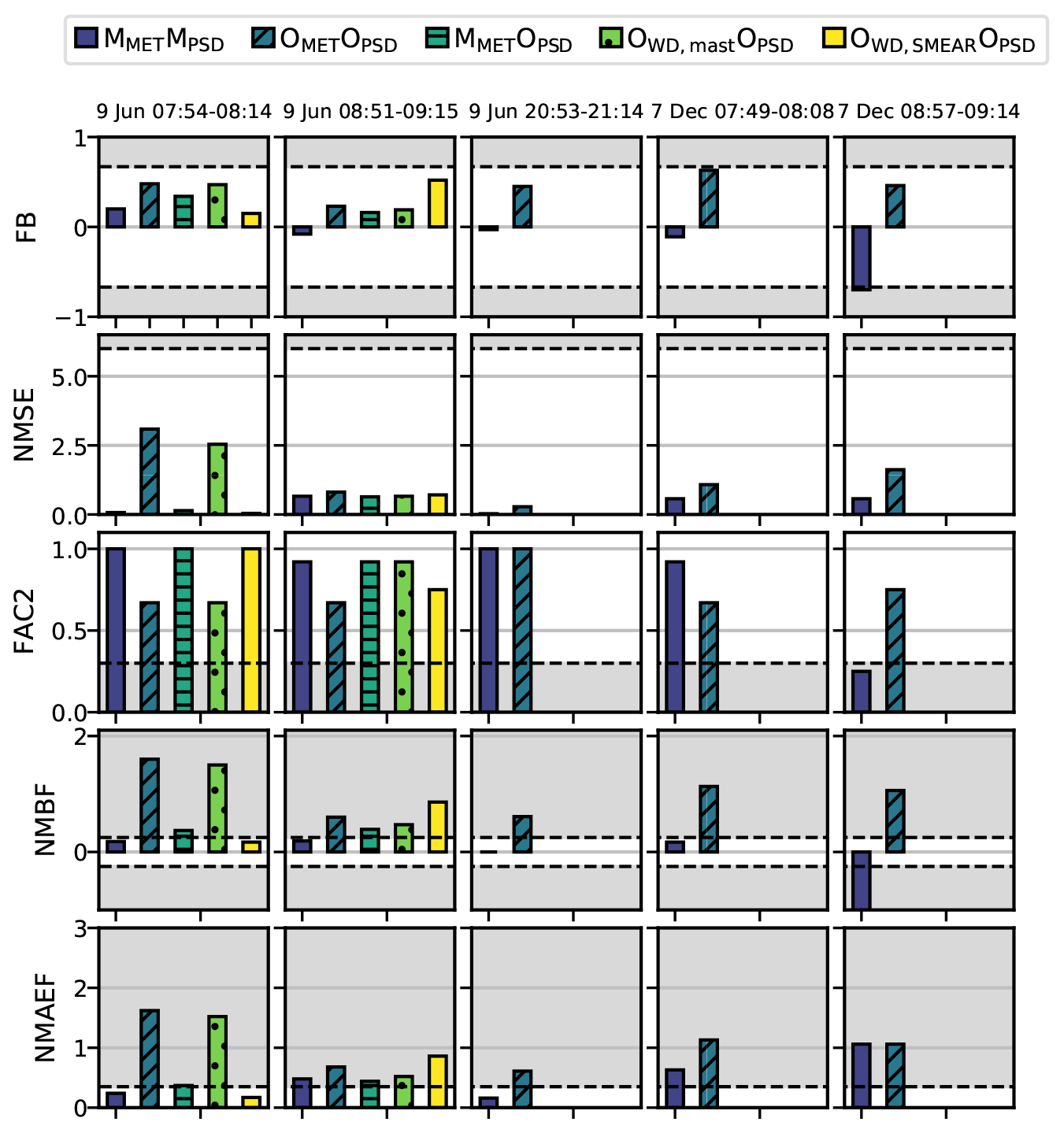
In order to compare the data, both the mobile Sniffer measurements containing its geographical coordinates and the PALM data output have been horizontally aggregated to a 5 m×5 m grid, with a threshold of at least three measurement points per grid to calculate the median value. A comparison between the measured and modelled median total aerosol particle number concentration (Ntot) values is illustrated in Fig. 3. In general, the model captures the large concentration gradient between the main street (in the middle from northwest to southeast) and the side street on the northeast side of the main street. However, the model overestimates Ntot at the northwestern end of the Sniffer route at all simulation times, which is likely due to overestimation of the traffic emissions at an adjacent cross section. Ntot is well modelled also along the side street, except during the winter morning in MMETMPSD (Fig. 3d–e and i–j), when the model slightly underestimates Ntot. The performance measures in simulating the horizontal distribution of Ntot and whether the acceptance criteria are fulfilled are shown in Fig. 4 for all simulation times. Overall, FB, NMSE and FAC2 show mostly acceptable model performance. However, NMBF often exceeds the acceptance criteria, showing that the model tends to over- or underestimate the observations by 25 % or more. NMAEF never fulfills the criteria, indicating that the absolute gross error between the observed and modelled values is always over 35 % larger than the mean observation.
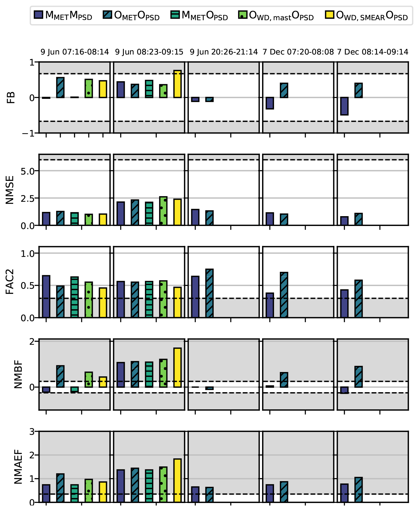
Figure 4Model performance for the horizontal distribution of Ntot using the FB, NMSE, FAC2, NMBF and NMAEF performance measures. The grey area indicates that the value exceeds the acceptance criteria given in Table 5. See Table 4 for the simulation names. Note that during the summer evening and winter morning, only two simulations have been conducted.
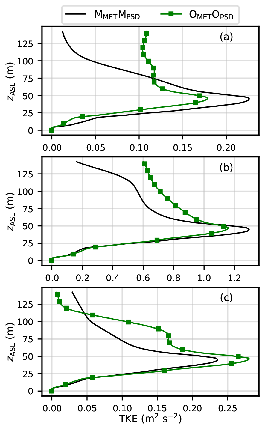
Figure 5The vertical profile of the mean turbulent kinetic energy (TKE) over the entire child domain for the (a) summer morning, (b) summer evening and (c) winter morning simulation. Each profile is temporally averaged over the whole simulation.
During the first hour in the summer morning, MMETMPSD performs better than OMETOPSD with respect to all performance measures. OMETOPSD clearly overestimates Ntot along the main street (Fig. 3k) despite a stronger temperature inversion in the MEPS model data (MMETMPSD) compared to the Kivenlahti (OMETOPSD) observations (Fig. 2c). This likely stems from the underestimation of the wind speeds above 217 m in OMETOPSD (Fig. 2a), which would lead to lower mechanical turbulence production and to lower mean turbulent kinetic energy (TKE) in OMETOPSD (Fig. 5a). During the second hour, no large differences in Ntot are observed, as the wind speed and direction of the input data become more equal.
Instead in the summer evening, OMETOPSD performs slightly better than MMETMPSD (e.g. FAC2=0.75 and FAC2=0.67, respectively), but both acquire good performance values and even NMBF is within the acceptance criteria. This is surprising considering the clearly stronger winds in MEPS at z<200 m than what is observed on the Kivenlahti mast. Yet, MEPS predicts a more stable stratification, which leads to nearly equal TKE values (Fig. 5b). This can justify why the difference in the spatial variability of aerosol particle concentrations between MMETMPSD and OMETOPSD is not that large.
During the winter morning, MMETMPSD fulfills the acceptance criteria during the first hour, except for NMAEF, and performs better than OMETOPSD. However, during the second hour, the difference is small. Interestingly, FAC2 is higher for OMETOPSD than MMETMPSD over the whole simulation. Contrary to the summer evening, MEPS predicts clearly lower wind speeds in the winter morning, which would lead to weaker mixing, but at the same time the observed temperature inversion on the Kivenlahti mast is stronger than the modelled by MEPS especially during the first hours. Hence, the stronger stability and suppression of turbulence (Fig. 5c) can explain the higher concentrations in OMETOPSD. However, it should be noted that for the first hour the differences in the model absolute error between MMETMPSD and OMETOPSD are not significant, and for the second hour a Student's t test cannot be performed (see Table S2 in the Supplement).
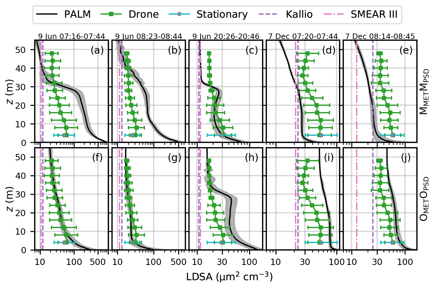
Figure 6Measured (marker with error bar) and modelled (black line and grey-shaded area) LDSA of aerosol particles at the supersite for the summer morning (a, f for the first and b, g for the second hour), summer evening (c, h) and winter morning (d, i for the first and e, j for the second hour). The first row shows MMETMPSD and the second OMETOPSD. The figure shows the geometric mean (measured: marker; modelled: solid line) and geometric standard deviation (measured: error bar; modelled: shaded area). Dashed lines show the geometric mean at the urban background monitoring sites in Kallio and SMEAR III.
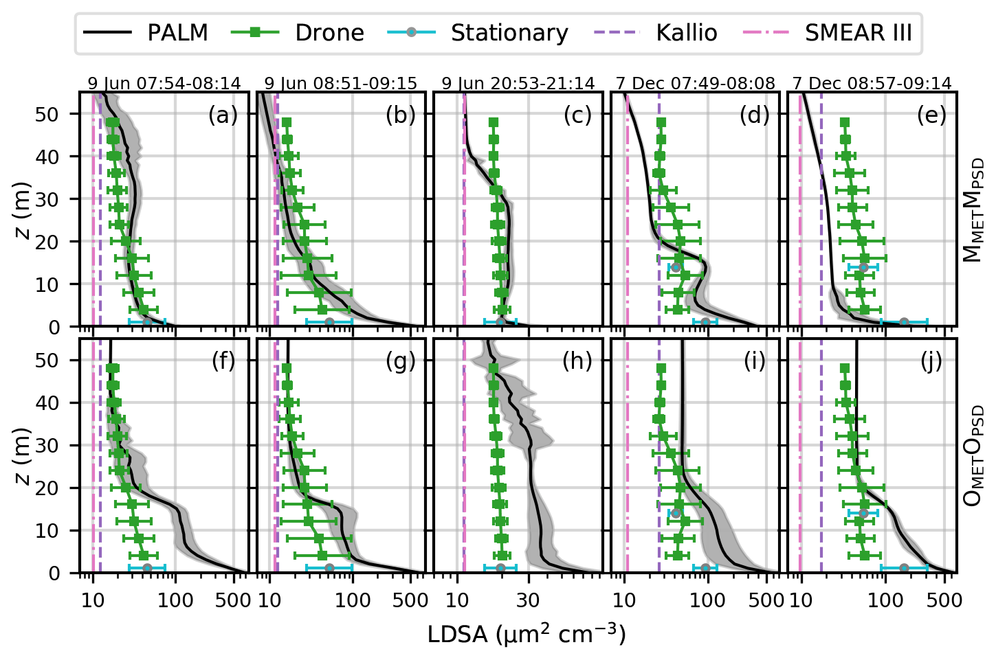
Figure 7Measured (marker with error bar) and modelled (black line and grey-shaded area) LDSA of aerosol particles opposite the supersite for the summer morning (a, f for the first and b, g for the second hour), summer evening (c, h) and winter morning (d, i for the first and e, j for the second hour). The first row shows MMETMPSD and the second OMETOPSD. The figure shows the geometric mean (measured: marker; modelled: solid line) and geometric standard deviation (measured: error bar; modelled: shaded area). Dashed lines show the geometric mean at the urban background monitoring sites in Kallio and SMEAR III.

5.3 Vertical profile of the lung-deposited surface area
The modelled vertical profile of alveolar LDSA is evaluated against the observed one over a 5 m×5 m area next to the supersite on the northern side of the container (Fig. 6) and opposite the supersite on the other side of the main street (Fig. 7). In the summer morning, MMETMPSD performs well opposite the supersite (Figs. 7a–b and 9) especially during the first hour, but it clearly overestimates LDSA at the supersite (Figs. 6a–b and 8). On the contrary, OMETOPSD successfully reproduces the LDSA profile at the supersite (Fig. 6f–g) but not opposite it (Fig. 7f–g). This can be explained by the wind direction: according to the meteorological boundary condition analysis in Sect. 4, the wind direction predicted by MEPS is more westerly than the one observed at Kivenlahti. Therefore, a canyon vortex forming in the main street canyon pushes pollutants upwind to the western side of the street in MMETMPSD. On the other hand, the opposite is observed for OMETOPSD for which the wind direction is more from the north. In the summer evening, MMETMPSD fulfills all acceptance criteria, while OMETOPSD overestimates LDSA on both sides of the street canyon. This is contradictory to the horizontal distribution of Ntot, based on which OMETOPSD showed better performance. In the winter morning, OMETOPSD shows slightly better performance at the supersite, whereas MMETMPSD underestimates LDSA, but it also has a lower background concentration. Instead, opposite the supersite, OMETOPSD clearly overestimates LDSA below the building height. For the summer evening and winter morning, the differences in the shape of the vertical LDSA profiles are not as notable as in the summer morning, which can be explained by the good correspondence of the Kivenlahti wind direction observations to the MEPS data.
5.4 Aerosol size distribution
Figure 10 illustrates the observed and modelled PSD for MMETMPSD separately along the main and side streets, at the supersite and opposite it, and in the background during the first hour of the summer morning on 9 June. In addition to the Sniffer measurements with EEPS and ELPI, the modelled values are compared against differential mobility particle sizer (DMPS) measurements at the supersite and SMEAR III. The model successfully reproduces PSD along the main street and specifically at the supersite, for which FB, NMSE and FAC2 are within the acceptance criteria (see Table S3 in the Supplement). Also in the background, the Sniffer measurements agree with the model based on FB, NMSE and FAC2 even though the concentration of the smallest (the mean bin diameter Dmid<25 nm) aerosol particles is underestimated. Instead, along the side street, the modelled values are clearly lower than the observed and, for instance, based on NMBF the model underestimates the EEPS and ELPI observations by a factor of 3.45 and 5.48, respectively.

Figure 10The mean aerosol number size distribution dN∕dlog D (cm−3) at different parts of the domain at z=1.5 m for MMETMPSD on the morning of 9 June at 07:16–08:14 LT. Modelled values are shown with a solid black line and Sniffer measurements with green lines: solid with filled squares for EEPS and dotted with empty squares for ELPI. Stationary DMPS measurements are shown with a solid light-green line with circles (SS indicates a supersite) and dotted pink line (SMEAR III). Note that for this observation period no stationary Sniffer measurements are available opposite the supersite.
Comparing the two simulations with different boundary conditions, MMETMPSD performs better along the main street and hence also at the supersite and opposite it during the first hour of the summer morning (Tables S3 and S4). However, during the second hour, the difference between MMETMPSD and OMETOPSD is minor, which was also observed for the horizontal distribution of Ntot. OMETOPSD, which uses the observed background PSD as boundary conditions, performs better along the side street and in the background. This is also observed in the summer evening (Tables S8 and S9) and winter morning (Tables S10 and S11). In the summer evening, both MMETMPSD and OMETOPSD perform equally well along the main street and equally poorly at the supersite overestimating the EEPS measurements by a factor of 3.68–4.36 based on NMBF (Tables S8 and S9). In the winter morning, MMETMPSD produces better results than OMETOPSD along the main street. Instead, at the supersite, both MMETMPSD and OMETOPSD perform equally well and fulfill the acceptance criteria for FB, NMSE and FAC2 (Tables S10 and S11).
Table 6Performance of the modelled aerosol chemical composition at the supersite on the morning of 9 June between 07:16 and 09:15 LT. See Fig. 4 for further description.
5.5 Aerosol chemical composition
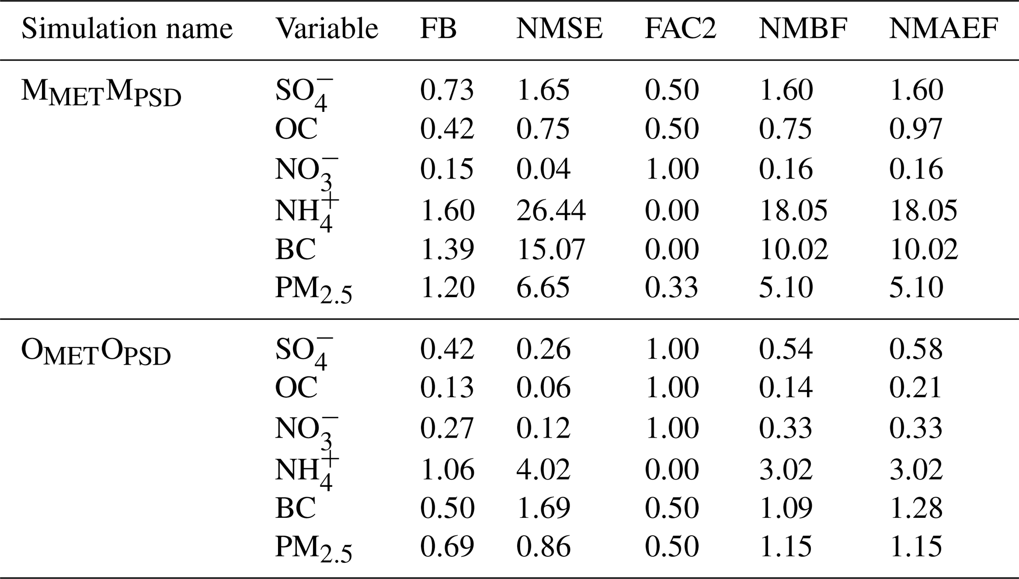
The chemical composition of aerosols was measured at the supersite by an ACSM (aerosol chemical speciation monitor) and the black carbon (BC) concentration by a MAAP (multi-angle absorption photometer; see Table S1 in the Supplement). Additionally, the Sniffer measured BC within PM1. In general, the modelled and observed horizontal distributions of BC compare tolerably well based on the performance measures FB, NMSE and FAC2, while NMBF and NMAEF are not within the acceptance criteria (see Fig. S13 in the Supplement). Overall, the performance is best for MMETMPSD in the summer morning during the first hour. In the summer and winter mornings, OMETOPSD suffers from high positive bias and absolute error and MMETMPSD in the winter morning from high absolute error. Instead, in the summer evening, both simulations show NMSE and FAC2 within the acceptance criteria but still overestimate BC. Comparison to the measured chemical composition of aerosols at the supersite (Tables 6 and S12–13) shows that the modelled concentration of organic carbon (OC) is in general on the right order of magnitude. Furthermore, in the summer morning (Table 6), especially the concentrations of sulfates () and nitrates (), and also BC and PM2.5 are correctly reproduced by OMETOPSD, while ammonium () is highly overestimated especially by MMETMPSD (NMBF=18.05). In the summer evening (Table S12), MMETMPSD corresponds better to observations than OMETOPSD and correctly reproduces , OC and PM2.5, while overestimating the rest. Also in the winter morning (Table S13), MMETMPSD performs slightly better than OMETOPSD in modelling OC and PM2.5 on the right order of magnitude, but MMETMPSD still overestimates the mass concentrations of the other chemical components by a factor of around 2.7–6.5. Hence, the difference in the chemical composition is not systematic. Comparing modelled values with point observations in a street canyon is very sensitive to the correct wind direction because a perpendicular wind component leads to accumulation of pollutants on the leeward side of the street canyon. As the vertical dispersion of LDSA was also shown sensitive to the wind direction, the results of the performance of modelling the correct chemical composition correspond to those of the vertical dispersion of LDSA (see Sect. 5.3).
6.1 Background aerosol size distribution
Sensitivity of the modelled aerosol concentrations to the background PSD is investigated by applying the modelled PSD (MMETMPSD) from ADCHEM and the observed PSD at SMEAR III (MMETOPSD) as the background PSD. Regarding all variables used in the evaluation (Ntot, LDSA, PSD and aerosol chemical composition), only minor differences are observed between MMETMPSD and MMETOPSD. For instance, for the horizontal distribution of Ntot, and FB=0.01, and NMSE=1.17 and NMSE=1.15, respectively (see Fig. 4). The difference in the horizontal distribution of Ntot (Fig. 11b) is mainly within −20–20 % with slightly higher (lower) concentrations in the southern (northern) part of the domain. This difference stems from roughly 80 % lower observed than modelled background Ntot, and thus the air being advected from northwest is cleaner in MMETOPSD compared to MMETMPSD.
Similar to the horizontal distribution, the vertical profile of LDSA for MMETOPSD does not differ from MMETMPSD within the street canyon (Fig. 12). Only a small decrease in model performance is observed opposite the supersite when applying the observed PSD as the boundary condition (e.g. FB is increased from 0.20 to 0.34 and NMSE from 0.07 to 0.14 during the first hour; Fig. 9). However, above z>30 m, the difference gradually approaches 65 %–160 %, i.e. the relative difference in the background Ntot between the modelled ADCHEM values and SMEAR III observations.
With respect to PSD, MMETMPSD and MMETOPSD perform mostly equally well or poorly, except for slightly better performance of MMETOPSD on the side street. The wind speed and/or direction influence the modelled PSD more than the background PSD (see Fig. S14 in the Supplement).
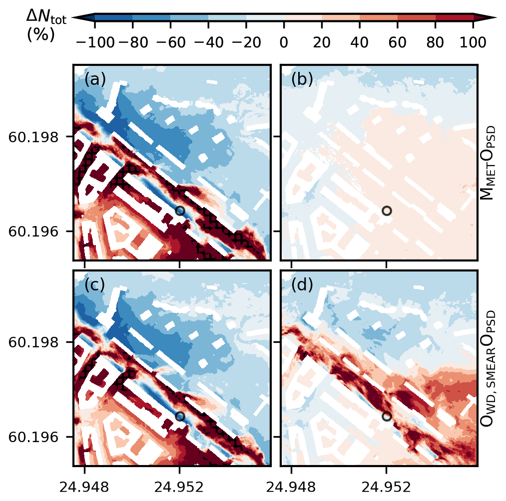
Figure 11Relative difference in the total aerosol number concentration (ΔNtot) at z=2.5 m on the morning of 9 June between 07:16 and 09:15 LT compared to MMETMPSD for (a) OMETOPSD, (b) MMETOPSD, (c) OWD,mastOPSD and (d) OWD,SMEAROPSD. The area with black crosses shows . Buildings shown with white and black circles denote the locations of the supersites. Note that ΔNtot is shown here for the whole simulation and not separately for each hour.

Figure 12Relative difference in the lung-deposited surface area (ΔLDSA) of aerosol particles compared to MMETMPSD at the supersite (a, c) and opposite the supersite (b, d) on the morning of 9 June. The figure shows the difference in the geometric mean for OMETOPSD (solid line with empty circles), MMETOPSD (dashed line with empty squares), OWD,mastOPSD (dash–dot line with filled squares) and OWD,SMEAROPSD (dotted line with filled squares).
6.2 Background meteorological conditions
In Sect. 5, the simulation using the observed data as boundary conditions (OMETOPSD) was shown to perform worse than when using the modelled MEPS data (MMETMPSD) in the summer morning. As the observed wind speed at Kivenlahti and the one modelled by MEPS differ (see Sect. 4), we separately investigate the model sensitivity to the incoming wind direction.
In general, OMETOPSD and OWD,mastOPSD, for which the meteorological boundary conditions are taken from MEPS but the incoming wind direction is replaced with the one measured on the Kivenlahti mast, result in a similar pattern for the difference in the horizontal distribution of Ntot compared to MMETMPSD (Fig. 11a, c). However, the differences are larger for OMETOPSD, for which the incoming upper-level wind speed is up to 2 m s−1 slower than in OWD,mastOPSD during the first hour (Fig. 2a). This results in the aerosol particles being transported more to the southwest side of the main street. As the wind is more from the north in OMETOPSD than in OWD,mastOPSD, also the impact of wind direction on the street-canyon vortex along the main street is observed by clearly lower (higher) Ntot on the southern (northern) side of the street canyon. The similar patterns of ΔNtot for OMETOPSD and OWD,mastOPSD but the higher absolute values of ΔNtot for OMETOPSD indicate that the horizontal distribution is strongly controlled by the wind direction, while the absolute values depend on the wind speed. Instead, OWD,SMEAROPSD, for which the wind direction is from SMEAR III and does not vary with height, shows clearly higher concentrations (up to +150 %) along the main street but smaller differences in its surroundings (−40–80 %).
Replacing the modelled wind direction with the one observed on the Kivenlahti mast (OWD,mastOPSD) or SMEAR III (OWD,SMEAROPSD) improves the model performance for the horizontal distribution of Ntot during the first summer morning hour (Fig. 4). However, for the second hour, OWD,SMEAROPSD is shown to perform even worse than OMETOPSD based on a lower FAC2 and higher NMBF and NMAEF. During the first hour, OWD,SMEAROPSD performs better than OWD,mastOPSD based on FB, NMBF and NMAEF, indicating that there is more bias in OWD,mastOPSD, while during the second hour OWD,SMEAROPSD performs better only based on NMSE. Presumably, the wind has too much of a westerly component in OWD,SMEAROPSD compared to the northerly winds in the MEPS and Kivenlahti data, which results in the traffic emissions downstream being flushed along the main street.
The observed vertical profile of LDSA at the supersite on the summer morning corresponds better to the one modelled by OMETOPSD and OWD,mastOPSD than MMETMPSD (Fig. 8). Hence, modifying the MEPS wind direction to correspond to the observed one at Kivenlahti increases the model performance. During the second hour, OWD,mastOPSD performs even slightly better than OMETOPSD (e.g. and , and NMSE=0.01 and NMSE=0.03). However, applying the wind direction from SMEAR III improves the model performance only for the first hour, while during the second hour OWD,SMEAROPSD performs the worst. Whereas OWD,mastOPSD results in lower (higher) LDSA than MMETMPSD below (above) m, OWD,SMEAROPSD shows higher values up to the building height (z=19 m) during the second hour, above which it gradually starts to follow the ΔLDSA for OWD,mastOPSD. Opposite the supersite, up to 5-fold values compared to MMETMPSD are observed in OMETOPSD and OWD,mastOPSD within the first hour (Fig. 12b), and the model performance is clearly decreased when using the observed wind direction from Kivenlahti (e.g. FB is increased from 0.20 to 0.47 and FAC2 decreased from 1.00 to 0.67; Fig. 9). Instead, OWD,SMEAROPSD performs better than MMETMPSD. Within the second hour, ΔLDSA compared to MMETMPSD is mainly within ±50 % below the building height, but above OWD,SMEAROPSD deviates from the other profiles showing 2-fold values. All ΔLDSA profiles gradually approach ∼100 %, which is a result of using different PSDs for MMETMPSD and for the rest of the simulations.
Similarly for the aerosol size distribution, changing the modelled wind direction by MEPS to the one measured at Kivenlahti improves model performance in the background and slightly decreases elsewhere during the first hour, whereas during the last hour PSD is modelled better along the side street and at the supersite (see Tables S3 and S6 in the Supplement). Applying the wind direction from SMEAR III generally does not improve model performance (Table S7). Along the main street, the difference in PSD is mainly governed by the emission, which is shown by the peak at Dmid≈30 nm in Fig. S14 (in the Supplement), while in the background ΔN follows the difference in the boundary conditions for aerosol particles.
This study provides an extensive evaluation of the SALSA2.0 module in the PALM model system 6.0 on simulating the horizontal distribution of aerosol particle number concentrations (Ntot), size distributions and black carbon concentrations and the vertical distribution of surface area (LDSA) in a complex urban environment. In addition, the aerosol chemical composition in a single measurement location is examined. Simulations are conducted under three different meteorological conditions: 2 h on a summer morning, 1 h on a summer evening and 2 h on a winter morning. The study also investigates the model sensitivity to the boundary conditions of meteorological variables and background aerosol concentrations during the different times.
Overall, the modelled aerosol concentrations compare well against observations. Indeed, the concentration fields are strongly influenced by the applied boundary conditions for the meteorological variables, while in this study the background PSD is shown to be less important. Especially the vertical profiles of LDSA are sensitive to the wind direction as it influences the formation and direction of the canyon vortex and thus the accumulation of pollutants on the leeward side of the street canyon. This also affects the model performance regarding the aerosol chemical composition, which is measured only at one point at the supersite. In general, the chemical composition is acceptably reproduced except for , which is highly overestimated at all times. Yet, the performance is not always systematic with the horizontal and vertical distributions. Furthermore, the horizontal distribution of Ntot is ruled by the prevailing wind speed and atmospheric stability, both of which control the turbulent mixing and ventilation. It is speculated that the wind speed and stability counteract each other in the summer and winter mornings, so that stronger stability can suppress TKE and turbulent mixing despite high wind speeds and consequent mechanical turbulence production, and vice versa.
Consequently, meteorological boundary conditions are particularly important for quantitative urban air quality modelling using LES, and therefore the inlet meteorology should be evaluated prior to conducting CFD simulations (Santiago et al., 2020). However, in our case, we are unable to thoroughly evaluate the modelled meteorology. In Santiago et al. (2020), the meteorological observations were made within the simulation domain, while in our case the closest measurements at SMEAR III are 800 m away from the supersite. Observations are available also from the Kivenlahti mast, which has several measurement levels but is located over 17 km away from the supersite and represents more semi-urban to rural area. Another problem with the Kivenlahti data is the lack of wind observations above 217 m in summer, which presumably leads to, for instance, underestimation of the incoming wind speed during the first simulation hour in the summer morning and around 21:00 LT in the summer evening. Consequently, neither of the observation datasets are optimal for evaluating the modelled meteorology or for providing meteorological boundary conditions for the simulations.
Of the aerosol metrics applied, LDSA directly estimates the health effect of aerosol exposure. The mean modelled LDSA concentration at z=4 m varies between 27 and 360 µm2 cm−3 at the supersite and between 20 and 250 µm2 cm−3 opposite the supersite, with the overall lowest LDSA opposite the supersite in MMETMPSD in the summer evening and highest at the supersite in MMETMPSD in the summer morning. As mentioned above, the wind direction is shown as a determining factor for accumulation of pollutants near the ground. The difference in near-ground LDSA between the supersite and opposite the supersite is the most pronounced in MMETMPSD during the first hour of the summer morning (360 and 37 µm2 cm−3, respectively). This large concentration gradient across the street illustrates the degree of error that can be made in the estimated outdoor-exposure level in epidemiological studies. Compared to urban background and traffic-monitoring stations (see Kuula et al., 2020, and references within), a street canyon allows for strong accumulation leading to high instantaneous concentrations.
However, LDSA is often overestimated near the ground in our simulations. One limitation of this study and in general in urban LES is omitting vehicle-induced turbulence (VIT), which would enhance vertical pollutant transport and mixing near the surface and very likely decrease concentrations near the ground. The research to include VIT in LES without extensive computational costs is ongoing and currently no freely available VIT model exists for LES. Neglecting the thermal turbulence in the simulations is another important limitation of our study. We acknowledge that omitting the influence of anthropogenic heat and heating by incoming solar radiation leads to overestimation of the vertical stability near the ground, which can partly explain the overestimation of the modelled surface concentrations. However, the spatial variability has been shown to be less dependent on a detailed heating distribution (Nazarian et al., 2018), and therefore the horizontal distribution is mainly determined by the predominant inflow conditions. Lastly, condensation of the biogenic volatile organic compounds on aerosol particles and their consecutive growth are not considered in PALM.
Performance measures calculated using the modelled Mi and observed Oi values. N is the number of samples.
FAC2 indicates the fraction of data that satisfy
The PALM code is freely available under the GNU General Public License v3. The exact model source code (revision 4416) is available at https://doi.org/10.5281/zenodo.4005366 (Kurppa, 2020a). MEPS model data are distributed under Norwegian license for public data (NLOD) and Creative Commons 4.0 BY International at https://thredds.met.no/thredds/catalog.html (last access: 18 February 2020) by the Norwegian Meteorological Institute.
All measurement data applied in the evaluation can be downloaded from https://doi.org/10.5281/zenodo.3828508 (Kurppa et al., 2020) and the input and output data, performance measures and source code modifications from https://doi.org/10.5281/zenodo.3824351 (Kurppa, 2020b). The scripts applied in the data analysis and model evaluation are freely available at https://doi.org/10.5281/zenodo.3839462 (Kurppa, 2020c), and the files and scripts for creating the PALM input data are available at https://doi.org/10.5281/zenodo.3839684 (Kurppa and Strömberg, 2020).
The supplement related to this article is available online at: https://doi.org/10.5194/gmd-13-5663-2020-supplement.
LJ and MK designed the concept of the study. MK prepared and conducted the LES simulations with contributions from AH, and PR conducted the ADCHEM simulations. MK, JS and SK contributed to the pre-processing of the used input datasets. LJ, HK, TR, JN, LP and HT planned the measurement campaign, and MK, HK, SK and HT conducted parts of the measurements. AB participated in post-processing the scripts of the Sniffer data. MK wrote the manuscript with contributions from all co-authors.
The authors declare that they have no conflict of interest.
The authors are very grateful to Aleksi Malinen and Sami Kulovuori from the Metropolia University of Applied Sciences for technical expertise and operation of the Sniffer, and to Aeromon Oy and Helsinki Region Environmental Services Authority (HSY) for collaboration in conducting the drone measurements.
This research has been supported by the Helsinki Metropolitan Region Urban Research Program, the Academy of Finland Centre of Excellence (grant no. 307331), Business Finland, the ERA-NET-COFUND project under ERA-PLANET (grant no. 689443) and the doctoral programme in atmospheric sciences (ATM-DP).
Open access funding provided by Helsinki University Library.
This paper was edited by Christoph Knote and reviewed by two anonymous referees.
Abhijith, K., Kumar, P., Gallagher, J., McNabola, A., Baldauf, R., Pilla, F., Broderick, B., Sabatino, S. D., and Pulvirenti, B.: Air pollution abatement performances of green infrastructure in open road and built-up street canyon environments – A review, Atmos. Environ., 162, 71–86, https://doi.org/10.1016/j.atmosenv.2017.05.014, 2017. a
Adam, M., Schikowski, T., Carsin, A. E., Cai, Y., Jacquemin, B., Sanchez, M., Vierkötter, A., Marcon, A., Keidel, D., Sugiri, D., Al Kanani, Z., Nadif, R., Siroux, V., Hardy, R., Kuh, D., Rochat, T., Bridevaux, P.-O., Eeftens, M., Tsai, M.-Y., Villani, S., Phuleria, H. C., Birk, M., Cyrys, J., Cirach, M., de Nazelle, A., Nieuwenhuijsen, M. J., Forsberg, B., de Hoogh, K., Declerq, C., Bono, R., Piccioni, P., Quass, U., Heinrich, J., Jarvis, D., Pin, I., Beelen, R., Hoek, G., Brunekreef, B., Schindler, C., Sunyer, J., Krämer, U., Kauffmann, F., Hansell, A. L., Künzli, N., and Probst-Hensch, N.: Adult lung function and long-term air pollution exposure. ESCAPE: a multicentre cohort study and meta-analysis, Eur. Respir. J., 45, 38–50, https://doi.org/10.1183/09031936.00130014, 2015. a
Andersen, Z. J., Bønnelykke, K., Hvidberg, M., Jensen, S. S., Ketzel, M., Loft, S., Sørensen, M., Tjønneland, A., Overvad, K., and Raaschou-Nielsen, O.: Long-term exposure to air pollution and asthma hospitalisations in older adults: a cohort study, Thorax, 67, 6–11, https://doi.org/10.1136/thoraxjnl-2011-200711, 2012. a
Arnold, F., Pirjola, L., Aufmhoff, H., Schuck, T., Lähde, T., and Hämeri, K.: First gaseous sulfuric acid measurements in automobile exhaust: Implications for volatile nanoparticle formation, Atmos. Environ., 40, 7097–7105, https://doi.org/10.1016/j.atmosenv.2006.06.038, 2006. a
Arnold, F., Pirjola, L., Rönkkö, T., Reichl, U., Schlager, H., Lähde, T., Heikkilä, J., and Keskinen, J.: First Online Measurements of Sulfuric Acid Gas in Modern Heavy-Duty Diesel Engine Exhaust: Implications for Nanoparticle Formation, Environ. Sci. Technol., 46, 11227–11234, https://doi.org/10.1021/es302432s, 2012. a
Auvinen, M. and Aarnio, M.: RasterH3D, available at: https://github.com/mjsauvinen/RasterH3D, last access: 20 June 2019. a
Auvinen, M. and Karttunen, S.: P4UL Pre- and Post-Processing Python Library for Urban LES Simulations, GitHub, available at: https://github.com/mjsauvinen/P4UL,last access: 28 June 2019. a
Auvinen, M., Boi, S., Hellsten, A., Tanhuanpää, T., and Järvi, L.: Study of realistic urban boundary layer turbulence with high-resolution large-eddy simulation, Atmosphere, 11, 201, https://doi.org/10.3390/atmos11020201, 2020. a
Baik, J.-J., Park, S.-B., and Kim, J.-J.: Urban Flow and Dispersion Simulation Using a CFD Model Coupled to a Mesoscale Model, J. Appl. Meteorol. Climatol., 48, 1667–1681, https://doi.org/10.1175/2009JAMC2066.1, 2009. a, b
Bengtsson, L., Andrae, U., Aspelien, T., Batrak, Y., Calvo, J., de Rooy, W., Gleeson, E., Hansen-Sass, B., Homleid, M., Hortal, M., Ivarsson, K.-I., Lenderink, G., Niemelä, S., Nielsen, K. P., Onvlee, J., Rontu, L., Samuelsson, P., Muñoz, D. S., Subias, A., Tijm, S., Toll, V., Yang, X., and Køltzow, M. Ø.: The HARMONIE-AROME Model Configuration in the ALADIN-HIRLAM NWP System, Mon. Weather Rev., 145, 1919–1935, https://doi.org/10.1175/MWR-D-16-0417.1, 2017. a
Brown, D. M., Wilson, M. R., MacNee, W., Stone, V., and Donaldson, K.: Size-Dependent Proinflammatory Effects of Ultrafine Polystyrene Particles: A Role for Surface Area and Oxidative Stress in the Enhanced Activity of Ultrafines, Toxicol. Appl. Pharm., 175, 191–199, https://doi.org/10.1006/taap.2001.9240, 2001. a
Burnett, R., Chen, H., Szyszkowicz, M., Fann, N., Hubbell, B., Pope, C. A., Apte, J. S., Brauer, M., Cohen, A., Weichenthal, S., Coggins, J., Di, Q., Brunekreef, B., Frostad, J., Lim, S. S., Kan, H., Walker, K. D., Thurston, G. D., Hayes, R. B., Lim, C. C., Turner, M. C., Jerrett, M., Krewski, D., Gapstur, S. M., Diver, W. R., Ostro, B., Goldberg, D., Crouse, D. L., Martin, R. V., Peters, P., Pinault, L., Tjepkema, M., van Donkelaar, A., Villeneuve, P. J., Miller, A. B., Yin, P., Zhou, M., Wang, L., Janssen, N. A. H., Marra, M., Atkinson, R. W., Tsang, H., Quoc Thach, T., Cannon, J. B., Allen, R. T., Hart, J. E., Laden, F., Cesaroni, G., Forastiere, F., Weinmayr, G., Jaensch, A., Nagel, G., Concin, H., and Spadaro, J. V.: Global estimates of mortality associated with long-term exposure to outdoor fine particulate matter, P. Natl. Acad. Sci. USA, 115, 9592–9597, https://doi.org/10.1073/pnas.1803222115, 2018. a
Chang, J. C. and Hanna, S. R.: Air quality model performance evaluation, Meteorol. Atmos. Phys., 87, 167–196, 2004. a
Chung, D. and McKeon, B. J.: Large-eddy simulation of large-scale structures in long channel flow, J. Fluid Mech., 661, 341–364, https://doi.org/10.1017/S0022112010002995, 2010. a
City of Helsinki: Map Service, available at: https://kartta.hel.fi/, last access: 19 December 2018a. a
City of Helsinki: Traffic rates in Helsinki, map, available at: https://www.hel.fi/static/liitteet/kaupunkiymparisto/liikenne-ja-kartat/kadut/liikennetilastot/autoliikenne/Autoliikennekartta.pdf (last access: 19 May 2020), 2018b (in Finnish). a
Damian, V., Sandu, A., Damian, M., Potra, F., and Carmichael, G. R.: The kinetic preprocessor KPP-a software environment for solving chemical kinetics, Comput. Chem. Eng., 26, 1567–1579, https://doi.org/10.1016/S0098-1354(02)00128-X, 2002. a
Enroth, J., Saarikoski, S., Niemi, J., Kousa, A., Ježek, I., Močnik, G., Carbone, S., Kuuluvainen, H., Rönkkö, T., Hillamo, R., and Pirjola, L.: Chemical and physical characterization of traffic particles in four different highway environments in the Helsinki metropolitan area, Atmos. Chem. Phys., 16, 5497–5512, https://doi.org/10.5194/acp-16-5497-2016, 2016. a
Finnish Meteorological Institute: Weather observations: Kivenlahti mast, available at: http://opendata.fmi.fi/wfs, last access: 18 February 2020. a
Fishpool, G. M., Lardeau, S., and Leschziner, M. A.: Persistent Non-Homogeneous Features in Periodic Channel-Flow Simulations, Flow Turbul. Combust., 83, 323–342, https://doi.org/10.1007/s10494-009-9209-z, 2009. a
García-Sánchez, C., van Beeck, J., and Gorlé, C.: Predictive large eddy simulations for urban flows: Challenges and opportunities, Build. Environ., 139, 146–156, https://doi.org/10.1016/j.buildenv.2018.05.007, 2018. a, b
Gronemeier, T. and Sühring, M.: On the Effects of Lateral Openings on Courtyard Ventilation and Pollution—A Large-Eddy Simulation Study, Atmosphere, 10, 63, https://doi.org/10.3390/atmos10020063, 2019. a
Hackbusch, W.: Multi-grid methods and applications, 1st edn.), Springer-Verlag, Berlin Heidelberg, 1985. a
Hanna, S. and Chang, J.: Acceptance criteria for urban dispersion model evaluation, Meteorol. Atmos. Phys., 116, 133–146, https://doi.org/10.1007/s00703-011-0177-1, 2012. a, b
Heinze, R., Moseley, C., Böske, L. N., Muppa, S. K., Maurer, V., Raasch, S., and Stevens, B.: Evaluation of large-eddy simulations forced with mesoscale model output for a multi-week period during a measurement campaign, Atmos. Chem. Phys., 17, 7083–7109, https://doi.org/10.5194/acp-17-7083-2017, 2017. a
Hellsten, A., Ketelsen, K., Barmpas, F., Tsegas, G., Moussiopoulos, N., and Raasch, S.: Nested multi-scale system implemented in the PALM large-eddy simulation model, in: Air pollution modelling and its application XXV, edited by: Klemens, M. and Kallos, G., Springer, 287–292, 2017. a
Helsinki Region Environmental Services Authority: Descriptions for the stationary monitoring stations, available at: https://www.hsy.fi/fi/asiantuntijalle/ilmansuojelu/mittausasematpks/Documents/Pysyvien mittausasemien kuvaukset.pdf, last access: 27 April 2020 (in Finnish). a
Hietikko, R., Kuuluvainen, H., Harrison, R. M., Portin, H., Timonen, H., Niemi, J. V., and Rönkkö, T.: Diurnal variation of nanocluster aerosol concentrations and emission factors in a street canyon, Atmos. Environ., 189, 98–106, https://doi.org/10.1016/j.atmosenv.2018.06.031, 2018. a
Huang, C., Wang, H. L., Li, L., Wang, Q., Lu, Q., de Gouw, J. A., Zhou, M., Jing, S. A., Lu, J., and Chen, C. H.: VOC species and emission inventory from vehicles and their SOA formation potentials estimation in Shanghai, China, Atmos. Chem. Phys., 15, 11081–11096, https://doi.org/10.5194/acp-15-11081-2015, 2015. a
Hussain, M., Madl, P., and Khan, A.: Lung deposition predictions of airborne particles and the emergence of contemporary diseases, Part-I, Health, 2, 51–59, 2011. a
Järvi, L., Hannuniemi, H., Hussein, T., Junninen, H., Aalto, P., Hillamo, R., Mäkelä, T., Keronen, P., Siivola, E., Vesala, T., and Kulmala, M.: The urban measurement station SMEAR III: Continuous monitoring of air pollution and surface-atmosphere interactions in Helsinki, Finland, Boreal Environ. Res., 14, 86–109, 2009. a
Jöckel, P., Kerkweg, A., Pozzer, A., Sander, R., Tost, H., Riede, H., Baumgaertner, A., Gromov, S., and Kern, B.: Development cycle 2 of the Modular Earth Submodel System (MESSy2), Geosci. Model Dev., 3, 717–752, https://doi.org/10.5194/gmd-3-717-2010, 2010. a
Junninen, H., Lauri, A., Keronen, P., Aalto, P., Hiltunen, V., Hari, P., and Kulmala, M.: Smart-SMEAR: on-line data exploration and visualization tool for SMEAR stations, Boreal Environ. Res., 14, 447–457, 2009. a
Kampa, M. and Castanas, E.: Human health effects of air pollution, Environ. Pollut., 151, 362–367, https://doi.org/10.1016/j.envpol.2007.06.012, 2008. a
Kelly, F. J. and Fussell, J. C.: Size, source and chemical composition as determinants of toxicity attributable to ambient particulate matter, Atmos. Environ., 60, 504–526, https://doi.org/10.1016/j.atmosenv.2012.06.039, 2012. a
Kokkola, H., Korhonen, H., Lehtinen, K. E. J., Makkonen, R., Asmi, A., Järvenoja, S., Anttila, T., Partanen, A.-I., Kulmala, M., Järvinen, H., Laaksonen, A., and Kerminen, V.-M.: SALSA – a Sectional Aerosol module for Large Scale Applications, Atmos. Chem. Phys., 8, 2469–2483, https://doi.org/10.5194/acp-8-2469-2008, 2008. a, b
Kurppa, M.: Source code of the PALM model system (revision 4416) (Version r4416), Zenodo, https://doi.org/10.5281/zenodo.4005366, 2020. a
Kurppa, M.: Model input and output, performance measures and modifications in the source code for PALM simulations on Mäkelänkatu in Helsinki, Finland, Zenodo, https://doi.org/10.5281/zenodo.3824351, 2020a. a
Kurppa, M.: Python scripts for evaluating PALM simulations against mobile air quality observations on Mäkelänkatu in Helsinki, Finland, Zenodo, https://doi.org/10.5281/zenodo.3839462, 2020b. a
Kurppa, M. and Strömberg, J.: Input files and scripts for creating PALM simulation input files on Mäkelänkatu in Helsinki, Finland, Zenodo, https://doi.org/10.5281/zenodo.3839684, 2020. a
Kurppa, M., Hellsten, A., Roldin, P., Kokkola, H., Tonttila, J., Auvinen, M., Kent, C., Kumar, P., Maronga, B., and Järvi, L.: Implementation of the sectional aerosol module SALSA2.0 into the PALM model system 6.0: model development and first evaluation, Geosci. Model Dev., 12, 1403–1422, https://doi.org/10.5194/gmd-12-1403-2019, 2019. a, b, c, d, e, f
Kurppa, M., Balling, A., Karttunen, S., Kuuluvainen, H., Järvi, L., Niemi, J. V., Pirjola, L., Rönkkö, T., and Timonen, H.: Mobile and stationary air pollution measurements around an air quality monitoring site on Mäkelänkatu in Helsinki, Finland, Zenodo, https://doi.org/10.5281/zenodo.3828508, 2020. a
Kuula, J., Kuuluvainen, H., Niemi, J. V., Saukko, E., Portin, H., Kousa, A., Aurela, M., Rönkkö, T., and Timonen, H.: Long-term sensor measurements of lung deposited surface area of particulate matter emitted from local vehicular and residential wood combustion sources, Aerosol Sci. Tech., 54, 190–202, https://doi.org/10.1080/02786826.2019.1668909, 2020. a, b
Kuuluvainen, H., Poikkimäki, M., Järvinen, A., Kuula, J., Irjala, M., Maso, M. D., Keskinen, J., Timonen, H., Niemi, J. V., and Rönkkö, T.: Vertical profiles of lung deposited surface area concentration of particulate matter measured with a drone in a street canyon, Environ. Pollut., 241, 96–105, https://doi.org/10.1016/j.envpol.2018.04.100, 2018. a, b
Kwak, K.-H., Baik, J.-J., Ryu, Y.-H., and Lee, S.-H.: Urban air quality simulation in a high-rise building area using a CFD model coupled with mesoscale meteorological and chemistry-transport models, Atmos. Environ., 100, 167–177, https://doi.org/10.1016/j.atmosenv.2014.10.059, 2015. a, b
Lelieveld, J., Evans, J. S., Fnais, M., Giannadaki, D., and Pozzer, A.: The contribution of outdoor air pollution sources to premature mortality on a global scale, Nature, 525, 367–371, https://doi.org/10.1038/nature15371, 2015. a
Lelieveld, J., Klingmüller, K., Pozzer, A., Pöschl, U., Fnais, M., Daiber, A., and Münzel, T.: Cardiovascular disease burden from ambient air pollution in Europe reassessed using novel hazard ratio functions, Eur. Heart J., 40, 1590–1596, https://doi.org/10.1093/eurheartj/ehz135, 2019. a
Letzel, M. O., Helmke, C., Ng, E., An, X., Lai, A., and Raasch, S.: LES case study on pedestrian level ventilation in two neighbourhoods in Hong Kong, Meteorol. Z., 21, 575–589, https://doi.org/10.1127/0941-2948/2012/0356, 2012. a, b
Liu, Y., Miao, S., Zhang, C., Cui, G., and Zhang, Z.: Study on micro-atmospheric environment by coupling large eddy simulation with mesoscale model, J. Wind Eng. Ind. Aerod., 107–108, 106–117, https://doi.org/10.1016/j.jweia.2012.03.033, 2012. a
Maronga, B., Gryschka, M., Heinze, R., Hoffmann, F., Kanani-Sühring, F., Keck, M., Ketelsen, K., Letzel, M. O., Sühring, M., and Raasch, S.: The Parallelized Large-Eddy Simulation Model (PALM) version 4.0 for atmospheric and oceanic flows: model formulation, recent developments, and future perspectives, Geosci. Model Dev., 8, 2515–2551, https://doi.org/10.5194/gmd-8-2515-2015, 2015. a
Maronga, B., Banzhaf, S., Burmeister, C., Esch, T., Forkel, R., Fröhlich, D., Fuka, V., Gehrke, K. F., Geletič, J., Giersch, S., Gronemeier, T., Groß, G., Heldens, W., Hellsten, A., Hoffmann, F., Inagaki, A., Kadasch, E., Kanani-Sühring, F., Ketelsen, K., Khan, B. A., Knigge, C., Knoop, H., Krč, P., Kurppa, M., Maamari, H., Matzarakis, A., Mauder, M., Pallasch, M., Pavlik, D., Pfafferott, J., Resler, J., Rissmann, S., Russo, E., Salim, M., Schrempf, M., Schwenkel, J., Seckmeyer, G., Schubert, S., Sühring, M., von Tils, R., Vollmer, L., Ward, S., Witha, B., Wurps, H., Zeidler, J., and Raasch, S.: Overview of the PALM model system 6.0, Geosci. Model Dev., 13, 1335–1372, https://doi.org/10.5194/gmd-13-1335-2020, 2020. a, b, c
Michioka, T., Sato, A., and Sada, K.: Large-eddy simulation coupled to mesoscale meteorological model for gas dispersion in an urban district, Atmos. Environ., 75, 153–162, https://doi.org/10.1016/j.atmosenv.2013.04.017, 2013. a
Miyakawa, T., Takegawa, N., and Kondo, Y.: Removal of sulfur dioxide and formation of sulfate aerosol in Tokyo, J. Geophys. Res.-Atmos., 112, D13209, https://doi.org/10.1029/2006JD007896, 2007. a
Müller, M., Homleid, M., Ivarsson, K.-I., Køltzow, M. A. Ø., Lindskog, M., Midtbø, K. H., Andrae, U., Aspelien, T., Berggren, L., Bjørge, D., Dahlgren, P., Kristiansen, J., Randriamampianina, R., Ridal, M., and Vignes, O.: AROME-MetCoOp: A Nordic Convective-Scale Operational Weather Prediction Model, Weather Forecast., 32, 609–627, https://doi.org/10.1175/WAF-D-16-0099.1, 2017. a
Nazarian, N., Martilli, A., and Kleissl, J.: Impacts of realistic urban heating, part I: spatial variability of mean flow, turbulent exchange and pollutant dispersion, Bound.-Lay. Meteorol., 166, 367–393, 2018. a
Nikolova, I., MacKenzie, A. R., Cai, X., Alam, M. S., and Harrison, R. M.: Modelling component evaporation and composition change of traffic-induced ultrafine particles during travel from street canyon to urban background, Faraday Discuss., 189, 529–546, https://doi.org/10.1039/C5FD00164A, 2016. a
Nordbo, A., Järvi, L., Haapanala, S., Moilanen, J., and Vesala, T.: Intra-City Variation in Urban Morphology and Turbulence Structure in Helsinki, Finland, Bound.-Lay. Meteorol., 146, 469–496, 2012. a
Norwegian Meteorological Institute: File Interpolation, Manipulation and EXtraction library, available at: https://wiki.met.no/fimex/start, last access: 12 June 2019a. a
Norwegian Meteorological Institute: MET Norway Thredds Service, available at: https://thredds.met.no/thredds/catalog.html, last access: 12 June 2019b. a
Ntziachristos, L., Samaras, Z., Kouridis, C., Samaras, C., Hassel, D., Mellios, G., McCrae, I., Hickman, J., Zierock, K.-H., Keller, M., Rexeis, M., Andre, M., Winther, M., Pastramas, N., Gorissen, N., Boulter, P., Katsis, P., Joumard, R., Rijkeboer, R., Geivanidis, S., and Hausberger, S.: EMEP/EEA air pollutant emission inventory guidebook, PART B: 1.A.3.b.i-iv Road transport, available at: https://www.eea.europa.eu/publications/emep-eea-guidebook-2016/part-b-sectoral-guidance-chapters/1-energy/1-a-combustion/1-a-3-b-i/view (last access: 18 June 2018), 2016. a, b
Oberdörster, G., Oberdörster, E., and Oberdörster, J.: Nanotoxicology: An Emerging Discipline Evolving from Studies of Ultrafine Particles, Environ. Health Persp., 113, 823–839, https://doi.org/10.1289/ehp.7339, 2005. a
Pirjola, L., Parviainen, H., Hussein, T., Valli, A., Hämeri, K., Aaalto, P., Virtanen, A., Keskinen, J., Pakkanen, T., Mäkelä, T., and Hillamö, R.: “Sniffer” – a novel tool for chasing vehicles and measuring traffic pollutants, Atmos. Environ., 38, 3625–3635, https://doi.org/10.1016/j.atmosenv.2004.03.047, 2004. a
Pirjola, L., Dittrich, A., Niemi, J. V., Saarikoski, S., Timonen, H., Kuuluvainen, H., Järvinen, A., Kousa, A., Rönkkö, T., and Hillamo, R.: Physical and Chemical Characterization of Real-World Particle Number and Mass Emissions from City Buses in Finland, Environ. Sci. Tech., 50, 294–304, https://doi.org/10.1021/acs.est.5b04105, 2016. a
Ramponi, R., Blocken, B., Laura, B., and Janssen, W. D.: CFD simulation of outdoor ventilation of generic urban configurations with different urban densities and equal and unequal street widths, Build. Environ., 92, 152–166, 2015. a
Roldin, P., Swietlicki, E., Massling, A., Kristensson, A., Löndahl, J., Eriksson, A., Pagels, J., and Gustafsson, S.: Aerosol ageing in an urban plume – implication for climate, Atmos. Chem. Phys., 11, 5897–5915, https://doi.org/10.5194/acp-11-5897-2011, 2011a. a
Roldin, P., Swietlicki, E., Schurgers, G., Arneth, A., Lehtinen, K. E. J., Boy, M., and Kulmala, M.: Development and evaluation of the aerosol dynamics and gas phase chemistry model ADCHEM, Atmos. Chem. Phys., 11, 5867–5896, https://doi.org/10.5194/acp-11-5867-2011, 2011b. a
Roldin, P., Ehn, M., Kurtén, T., Olenius, T., Rissanen, M. P., Sarnela, N., Elm, J., Rantala, P., Hao, L., Hyttinen, N., et al.: The role of highly oxygenated organic molecules in the Boreal aerosol-cloud-climate system, Nat. Commun., 10, 1–15, 2019. a, b
Salim, S. M., Buccolieri, R., Chan, A., and Sabatino, S. D.: Numerical simulation of atmospheric pollutant dispersion in an urban street canyon: Comparison between RANS and LES, J. Wind Eng. Ind. Aerod., 99, 103–113, https://doi.org/10.1016/j.jweia.2010.12.002, 2011. a, b
Santiago, J., Sanchez, B., Quaassdorff, C., de la Paz, D., Martilli, A., Martín, F., Borge, R., Rivas, E., Gómez-Moreno, F., Díaz, E., Artiñano, B., Yagüe, C., and Vardoulakis, S.: Performance evaluation of a multiscale modelling system applied to particulate matter dispersion in a real traffic hot spot in Madrid (Spain), Atmos. Pollut. Res., 11, 141–155, 2020. a, b, c, d, e
Saunders, S. M., Jenkin, M. E., Derwent, R. G., and Pilling, M. J.: Protocol for the development of the Master Chemical Mechanism, MCM v3 (Part A): tropospheric degradation of non-aromatic volatile organic compounds, Atmos. Chem. Phys., 3, 161–180, https://doi.org/10.5194/acp-3-161-2003, 2003. a
Steffens, J. T., Heist, D. K., Perry, S. G., and Zhang, K. M.: Modeling the effects of a solid barrier on pollutant dispersion under various atmospheric stability conditions, Atmos. Environ., 69, 76–85, https://doi.org/10.1016/j.atmosenv.2012.11.051, 2013. a
Stein, A. F., Draxler, R. R., Rolph, G. D., Stunder, B. J. B., Cohen, M. D., and Ngan, F.: NOAA’s HYSPLIT Atmospheric Transport and Dispersion Modeling System, B. Am. Meteorol. Soc., 96, 2059–2077, https://doi.org/10.1175/BAMS-D-14-00110.1, 2015. a
Tominaga, Y. and Stathopoulos, T.: CFD simulation of near-field pollutant dispersion in the urban environment: A review of current modeling techniques, Atmos. Environ., 79, 716–730, https://doi.org/10.1016/j.atmosenv.2013.07.028, 2013. a
UN: World Urbanization Prospects: The 2018 Revision (ST/ESA/SER.A/420), 2019. a
Urban Environment Division of the City of Helsinki, Helsinki Region Environmental Services Authority and Helsinki Region Municipalities: Traffic volumes in Helsinki 2017, map, available at: https://www.hel.fi/static/liitteet/kaupunkiymparisto/liikenne-ja-kartat/kadut/liikennetilastot/autoliikenne/Autoliikennekartta.pdf, last access: 18 June 2018 (in Finnish). a
VTT: LIPASTO unit emissions -database: Fuel properties, available at: http://lipasto.vtt.fi/yksikkopaastot/tunnusluvut/tunnusluvuttiee.htm (last access: 30 November 2018), 2017. a
VTT: ALIISA model, available at: http://lipasto.vtt.fi/aliisa/suoritejakaumat.htm, last access: 30 November 2018 (in Finnish). a
WHO: Ambient air pollution: A global assessment of exposure and burden of disease, World Health Organisation, 2016. a
Wicker, L. and Skamarock, W.: Time-splitting methods for elastic models using forward time schemes, Mon. Weather Rev., 130, 2088–2097, 2002. a
Williamson, J. H.: Low-Storage Runge-Kutta Schemes, J. Comput. Phys., 35, 48–56, https://doi.org/10.1016/0021-9991(80)90033-9, 1980. a
Wood, C. R., Järvi, L., Kouznetsov, R. D., Nordbo, A., Joffre, S., Drebs, A., Vihma, T., Hirsikko, A., Suomi, I., Fortelius, C., O'Connor, E., Moiseev, D., Haapanala, S., Moilanen, J., Kangas, M., Karppinen, A., Vesala, T., and Kukkonen, J.: An Overview of the Urban Boundary Layer Atmosphere Network in Helsinki, B. Am. Meteorol. Soc., 94, 1675–1690, https://doi.org/10.1175/BAMS-D-12-00146.1, 2013. a
Wyszogrodzki, A. A., Miao, S., and Chen, F.: Evaluation of the coupling between mesoscale-WRF and LES‐EULAG models for simulating fine-scale urban dispersion, Atmos. Res., 118, 324–345, https://doi.org/10.1016/j.atmosres.2012.07.023, 2012. a
Xie, Z.-T. and Castro, I. P.: LES and RANS for turbulent flow over arrays of wall-mounted obstacles, Flow Turbul. Combust., 76, 291–312, https://doi.org/10.1007/s10494-006-9018-6, 2006. a
Yu, S., Eder, B., Dennis, R., Chu, S.-H., and Schwartz, S. E.: New unbiased symmetric metrics for evaluation of air quality models, Atmos. Sci. Lett., 7, 26–34, https://doi.org/10.1002/asl.125, 2006. a, b, c
Zhao, Y., Saleh, R., Saliba, G., Presto, A. A., Gordon, T. D., Drozd, G. T., Goldstein, A. H., Donahue, N. M., and Robinson, A. L.: Reducing secondary organic aerosol formation from gasoline vehicle exhaust, P. Natl. Acad. Sci. USA, 114, 6984–6989, https://doi.org/10.1073/pnas.1620911114, 2017. a
Zhong, J., Nikolova, I., Cai, X., MacKenzie, A. R., Alam, M. S., Xu, R., Singh, A., and Harrison, R. M.: Traffic-induced multicomponent ultrafine particle microphysics in the WRF v3.6.1 large eddy simulation model: General behaviour from idealised scenarios at the neighbourhood-scale, Atmos. Environ., 223, 117213, https://doi.org/10.1016/j.atmosenv.2019.117213, 2020. a, b
- Abstract
- Introduction
- Measurements
- Simulations
- Comparison of the modelled and observed boundary conditions
- Evaluation of the air quality modelling results
- Sensitivity analysis
- Discussion and conclusions
- Appendix A: Performance measures
- Code and data availability
- Author contributions
- Competing interests
- Acknowledgements
- Financial support
- Review statement
- References
- Supplement