the Creative Commons Attribution 4.0 License.
the Creative Commons Attribution 4.0 License.
 | 12 Oct 2020
Newly developed aircraft routing options for air traffic simulation in the chemistry–climate model EMAC 2.53: AirTraf 2.0
Hiroshi Yamashita
Feijia Yin
Volker Grewe
Patrick Jöckel
Sigrun Matthes
Bastian Kern
Katrin Dahlmann
Christine Frömming
Aviation contributes to climate change, and the climate impact of aviation is expected to increase further. Adaptations of aircraft routings in order to reduce the climate impact are an important climate change mitigation measure. The air traffic simulator AirTraf, as a submodel of the European Center HAMburg general circulation model (ECHAM) and Modular Earth Submodel System (MESSy) Atmospheric Chemistry (EMAC) model, enables the evaluation of such measures. For the first version of the submodel AirTraf, we concentrated on the general setup of the model, including departure and arrival, performance and emissions, and technical aspects such as the parallelization of the aircraft trajectory calculation with only a limited set of optimization possibilities (time and distance). Here, in the second version of AirTraf, we focus on enlarging the objective functions by seven new options to enable assessing operational improvements in many more aspects including economic costs, contrail occurrence, and climate impact. We verify that the AirTraf setup, e.g., in terms of number and choice of design variables for the genetic algorithm, allows us to find solutions even with highly structured fields such as contrail occurrence. This is shown by example simulations of the new routing options, including around 100 North Atlantic flights of an Airbus A330 aircraft for a typical winter day. The results clearly show that AirTraf 2.0 can find the different families of optimum flight trajectories (three-dimensional) for specific routing options; those trajectories minimize the corresponding objective functions successfully. The minimum cost option lies between the minimum time and the minimum fuel options. Thus, aircraft operating costs are minimized by taking the best compromise between flight time and fuel use. The aircraft routings for contrail avoidance and minimum climate impact reduce the potential climate impact which is estimated by using algorithmic climate change functions, whereas these two routings increase the aircraft operating costs. A trade-off between the aircraft operating costs and the climate impact is confirmed. The simulation results are compared with literature data, and the consistency of the submodel AirTraf 2.0 is verified.
- Article
(4485 KB) - Full-text XML
-
Supplement
(2660 KB) - BibTeX
- EndNote


Climate impact due to aviation emissions is an important issue. Nowadays global aviation contributes only about 5 % to the anthropogenic climate impact (Skeie et al., 2009; Lee et al., 2009, 2010). However, the aviation's contribution to the climate impact is expected to increase further because global air traffic strongly grew in terms of revenue passenger kilometers (RPKs) by 7.4 % in 2016 compared to 2015 (ICAO, 2017). The aviation climate impact consists of carbon dioxide (CO2) emissions and of non-CO2 effects. The non-CO2 effects comprise nitrogen oxides (NOx) which lead to concentration changes of ozone and methane, water vapor (H2O), hydrocarbons (HC), carbon monoxide (CO), sulfur oxides (SOx), non-volatile particulate matter such as black carbon (BC), persistent linear contrails, and contrail-induced cirrus clouds (Wuebbles et al., 2007; Lee et al., 2009; Brasseur et al., 2016). These effects change the radiative balance of the Earth's climate system and cause radiative impact. The radiative impact potentially drives the climate system into a new state of equilibrium through temperature changes. Lee et al. (2009) stated that the CO2 emissions have the main impact and that the estimated radiative forcing (RF) of aviation CO2 in 2005 was 28.0 mW m−2 (15.2–40.8 mW m−2, 90 % likelihood range). The non-CO2 emissions and the induced clouds also have a large effect on RFs; for example, the estimated RFs in 2005 for total NOx and for persistent linear contrails were 12.6 mW m−2 (3.8–15.7 mW m−2, 90 % likelihood range) and 11.8 mW m−2 (5.4–25.6 mW m−2, 90 % likelihood range), respectively (Lee et al., 2009). In particular, the radiative impact of contrails remains uncertain, and recent studies report higher RF. Burkhardt and Kärcher (2011) estimated the contrail cirrus RF of 37.5 mW m−2 for the year 2002; Schumann et al. (2015) reported the RF of 63 mW m−2 for the year 2006; and Bock and Burkhardt (2016) estimated the RF of 56 mW m−2 for the year 2006. As for timescales of their impacts, the emitted CO2 becomes uniformly mixed in the whole atmosphere, and its perturbation remains for millennia. In contrast, the non-CO2 effects occur on short timescales, e.g., the emitted NOx remains for a few days to months; the contrails last several hours. Thus, the non-CO2 effects depend strongly on the ambient (local) atmospheric conditions (Fichter et al., 2005; Mannstein et al., 2005; Gauss et al., 2006; Grewe and Stenke, 2008; Frömming et al., 2012; Brasseur et al., 2016; Lund et al., 2017). To investigate measures for reducing the aviation climate impact, the impact of both CO2 and non-CO2 effects must be considered; therefore, geographic location, altitude, the time of released non-CO2 emissions and induced clouds, and corresponding local atmospheric conditions need to be considered.
In recent years, Grewe et al. (2017a, b) and Matthes et al. (2012, 2017) have proposed a climate-optimized routing as an important operational measure for reducing the aviation climate impact. This routing allows a significant reduction of the climate impact by optimizing flight routes to avoid regions where released emissions (including contrails) have a large climate impact. The climate-optimized routing is immediately applicable to present airline fleets, whereas other, more technological measures (e.g., efficient engines, blended wing–body configurations, and laminar flow controls; Green, 2005) require several years before implementation. Moreover, the routing can be used in addition to the technological measures for reducing the aviation climate impact.
Benefits of the climate-optimized routing have been examined before (Gierens et al., 2008; Schumann et al., 2011; Sridhar et al., 2013; Søvde et al., 2014; Lührs et al., 2016); for example, Frömming et al. (2013) and Grewe et al. (2014b) developed climate cost functions (CCFs) for the climate-optimized routing. They calculated global-average RFs resulting from local unit emissions (CO2, NOx, H2O, and contrails) over the North Atlantic for typical weather patterns by using the European Center HAMburg general circulation model (ECHAM) and Modular Earth Submodel System (MESSy) Atmospheric Chemistry (EMAC) model (Jöckel et al., 2010, 2016). Those RFs were used to calculate the global and temporal average near-surface temperature response over 20 years, which describes the climate impacts (i.e., future temperature changes) caused by those emissions on a per unit basis. The resulting data set is called the CCFs. The CCFs describe the climate impact which is induced by aviation's CO2 and non-CO2 effects (H2O, ozone, methane, ozone originating from methane changes, and contrails including the spread into contrail-cirrus), and the CCFs of those effects except CO2 are a function of geographic location, altitude, and time. Because of the long residence time of CO2, its impact is the same regardless of location, altitude, and time of emission. The obtained CCFs can be used as a measure of the climate impact of aviation and form the basis for the climate-optimized routing. Grewe et al. (2014a) calculated the CCFs for a winter day and optimized 1 d transatlantic air traffic (391 eastbound and 394 westbound flights) using the CCFs in the system for traffic assignment and analysis at macroscopic level (SAAM; Eurocontrol, 2012). They reported that the climate impact decreased by up to 25 % with a small increase in economic costs of less than 0.5 %. This revealed a great potential for the climate-optimized routing. On the other hand, a trade-off between climate impact and economic cost existed; i.e., the climate-optimized and the cost-optimized routings were conflicting strategies. Grewe et al. (2017b) extended this study and investigated the feasibility of the climate-optimized routing for realistic conditions. Similar transatlantic air traffic simulations (about 800 flights) were performed for five representative winter and three representative summer days, which took safety aspects into account. They found that a decrease in potential climate impact of 10 % was achieved at a cost increase of only 1 %.
The benefits of the climate-optimized routing were investigated by using different climate metrics. Ng et al. (2014) optimized flight trajectories for a total climate cost which was calculated by the absolute global temperature change potential (AGTP) (pulse AGTP values for three time horizons; Shine et al., 2005) due to CO2 emissions and contrails. A total of 960 transatlantic flights (482 eastbound and 478 westbound flights) were analyzed for a specific summer day. They reported that the climate-optimized routing reduced the total AGTP (for the medium-term climate goal of 50 years) by 38 % with an additional flight time of 3.1 % and with extra fuel use of 3.1 % for the eastbound flights, whereas the routing reduced the total AGTP by 20 % with an additional flight time of 3.0 % and with extra fuel use of 3.7 % for the westbound flights. Generally, aircraft operating costs depend on time and on fuel. Thus, those results indicate the aforementioned trade-off between climate impact and economic cost; this trade-off was also found for the short-term (25 years) and long-term (100 years) climate goals. Grewe et al. (2014a) compared the trade-off between economic costs and climate impact from the transatlantic air traffic simulations described above with respect to three climate metrics: the average temperature response with future increasing emissions (F-ATR20) and the absolute global warming potential with pulse emissions at a 20-year time horizon (P-AGWP20) for short-term climate impacts and P-AGWP100 (time horizon of 100 years) for long-term climate impacts. The trade-offs obtained with the three metrics were very similar. Although many studies show the benefit of the climate-optimized routing, this routing is not used for today's flight planning; today's aircraft routing focuses on minimum economic cost. However, if additional costs, such as environmental taxes, for aviation climate impact of CO2 and non-CO2 effects are included in the operating costs, a cost increase due to the climate-optimized routing is possibly compensated for (Grewe et al., 2017b). This inclusion can change the current routing strategy and incentivize airlines to introduce a climate-optimized flight planning.
Here we present an air traffic simulation model which serves as a basis for the following ultimate two aims: to investigate an eco-efficient aircraft routing strategy that reduces the climate impact of global air traffic over the next few decades and to estimate its mitigation gain for different aircraft routing strategies. For these aims, the submodel AirTraf (version 1.0) was developed as one of the submodels of EMAC (Yamashita et al., 2015, 2016). AirTraf can simulate global air traffic in EMAC (online) for various aircraft routing strategies (options). Every flight trajectory is optimized for a selected routing option under daily changing local atmospheric conditions. AirTraf can take into account where and when aviation emissions are released or contrails form. The road map for our overall study has been shown elsewhere (Grewe et al., 2017b; Matthes et al., 2017).
This paper presents a technical description of the new version of the submodel AirTraf 2.0. The simple aircraft routing options of great circle (minimum flight distance) and flight time (minimum time) were developed in the previous version of AirTraf 1.0 (Yamashita et al., 2016). In AirTraf 2.0, seven new aircraft routing options have been introduced: fuel use, NOx emissions, H2O emissions, contrail formation, simple operating cost (SOC), cash operating cost (COC), and climate impact estimated by the algorithmic climate change functions (aCCFs) (Van Manen, 2017; Yin et al., 2018b, 2020; Van Manen and Grewe, 2019). The climate change functions were previously referred to as the climate cost functions mentioned above. These options represent the objects to be minimized. Overall the nine options have been integrated into AirTraf 2.0, which enables air traffic simulations for the ultimate aims of our study (hereinafter the aircraft routing options are referred to simply as, e.g., the “fuel option”). Thus, the development described in this paper is an indispensable update. Moreover, this paper provides example applications of AirTraf 2.0. Some simulations of the nine routing options were carried out for transatlantic routes for a typical winter day. Optimum flight trajectories and characteristics of the routing options were analyzed.
Here we mention the importance of the variety of the routing options. Various routing options have been made available in AirTraf 2.0 because not only the climate and the cost options but also the other options are important subjects for air traffic routing studies. The time option is useful for delay recovery. Because delays cause costs to airlines, pilots are often forced to temporarily use the time option during a flight to maintain flight schedules, although the use of this option increases fuel costs (Cook et al., 2009). The NOx (Mulder and Ruijgrok, 2008) and contrail options (Fichter et al., 2005; Mannstein et al., 2005; Gierens et al., 2008; Sridhar et al., 2011; Schumann et al., 2011; Rosenow et al., 2017) have been examined as a routing strategy towards climate impact reduction. Moreover, conflicting scenarios (trade-offs) between different routing strategies have been studied; for example, avoiding contrail formation generally increases fuel use and CO2 emissions. Irvine et al. (2014) assessed the trade-off between contrail avoidance and increased CO2 emissions (∼ increased fuel use) for a single flight. AirTraf 2.0 enables the analysis of those subjects all at once because all the options are integrated. Normally, one or two specific routing options are available for a flight trajectory optimization in other models. Another aspect to be emphasized compared to other models is that AirTraf performs air traffic simulations not under International Standard Atmospheric (ISA) conditions and not under a fixed atmospheric condition for a specific day but under comprehensive atmospheric conditions which are calculated by EMAC; that is to say that AirTraf can simulate air traffic for long-term periods in EMAC, which enables one to examine effects of aircraft routing strategies on climate impact on a long-term timescale. Last but not least, the aCCFs are new proxies for the climate-optimized routing. An important aim of the AirTraf development is to verify the aCCFs themselves and the routing strategy based on the aCCFs (i.e., the climate option) in multi-annual (long-term) simulations (Yin et al., 2018b).
This paper is organized as follows. Section 2 describes an overview of AirTraf 2.0. Particularly, key changes in the model components are stated. Section 3 presents the results and discussion for the example applications of AirTraf 2.0 using the nine routing options. Section 4 verifies the consistency of the results with literature data. Finally, Sect. 5 concludes this study.
2.1 Chemistry–climate model EMAC
The EMAC model is a numerical chemistry and climate simulation system that includes submodels describing tropospheric and middle atmosphere processes and their interaction with oceans, land, and influences coming from anthropogenic emissions (Jöckel et al., 2010, 2016). It uses the second version of the Modular Earth Submodel System (MESSy2) to link multi-institutional computer codes. The core atmospheric model is the fifth generation European Center HAMburg general circulation model (ECHAM5; Roeckner et al., 2006). For the present study, we applied EMAC (ECHAM5 version 5.3.02 and MESSy version 2.53 updated from version 2.41 for AirTraf 1.0) in the T42L31ECMWF resolution, i.e., with a spherical truncation of T42 (corresponding to a quadratic Gaussian grid of approximately 2.8∘ by 2.8∘ in latitude and longitude) with 31 vertical hybrid pressure levels up to 10 hPa (middle of the uppermost layer). The namelist setup for ECHAM5 simulations (referred to the E5 setup, no chemistry) was employed. Moreover, the submodel AirTraf was coupled to the submodel CONTRAIL (version 1.0; Frömming et al., 2014) for the contrail option and to the submodel ACCF (version 1.0) for the climate option using the MESSy interfaces. Further information about MESSy, including the EMAC model system, is available from the MESSy Consortium website (http://www.messy-interface.org, last access: 17 September 2020).
2.2 Model components of submodel AirTraf
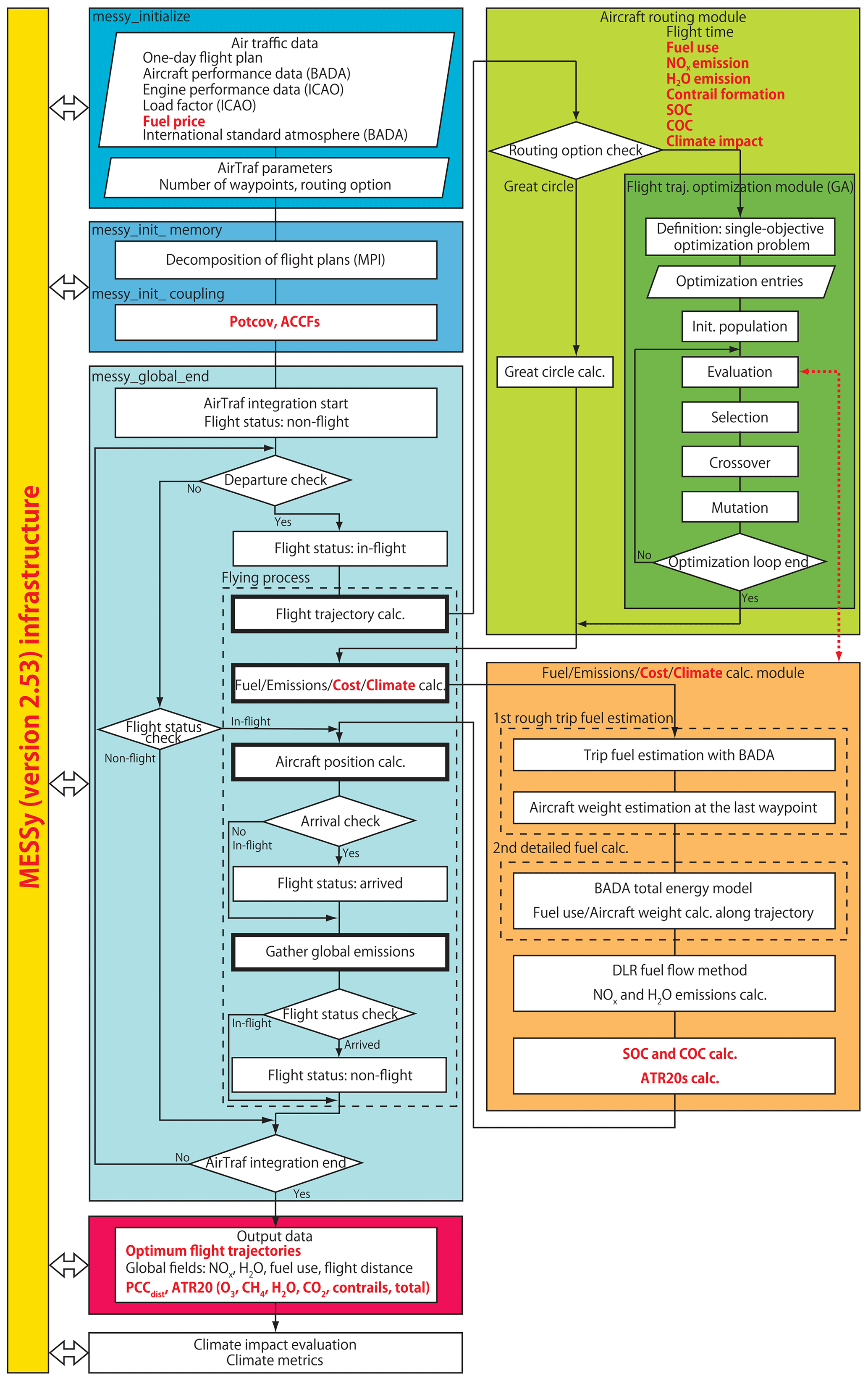
Figure 1Updated flowchart of the MESSy submodel AirTraf 2.0 (updates from AirTraf 1.0 are highlighted by red texts and arrows). MESSy as part of EMAC provides interfaces (yellow) to couple various submodels for data exchange, run control, and data input/output. AirTraf 2.0 is coupled to the submodel CONTRAIL (version 1.0; Frömming et al., 2014) and the submodel ACCF (version 1.0). Air traffic data and AirTraf parameters are imported in the initialization phase (messy_initialize, dark blue). AirTraf includes the flying process in messy_global_end (dashed box, light blue), which comprises four main computation procedures (bold black boxes). AirTraf uses three modules: the aircraft routing module (light green), the fuel–emissions–cost–climate calculation module (light orange), and the flight trajectory optimization module (dark green). Resulting optimum flight trajectories and global fields of flight properties are output (rose red).
Table 1Relevant data of an Airbus A330-301 aircraft and constant parameters applied for AirTraf 2.0. The column “New in V2.0” denotes parameters newly introduced in AirTraf 2.0.
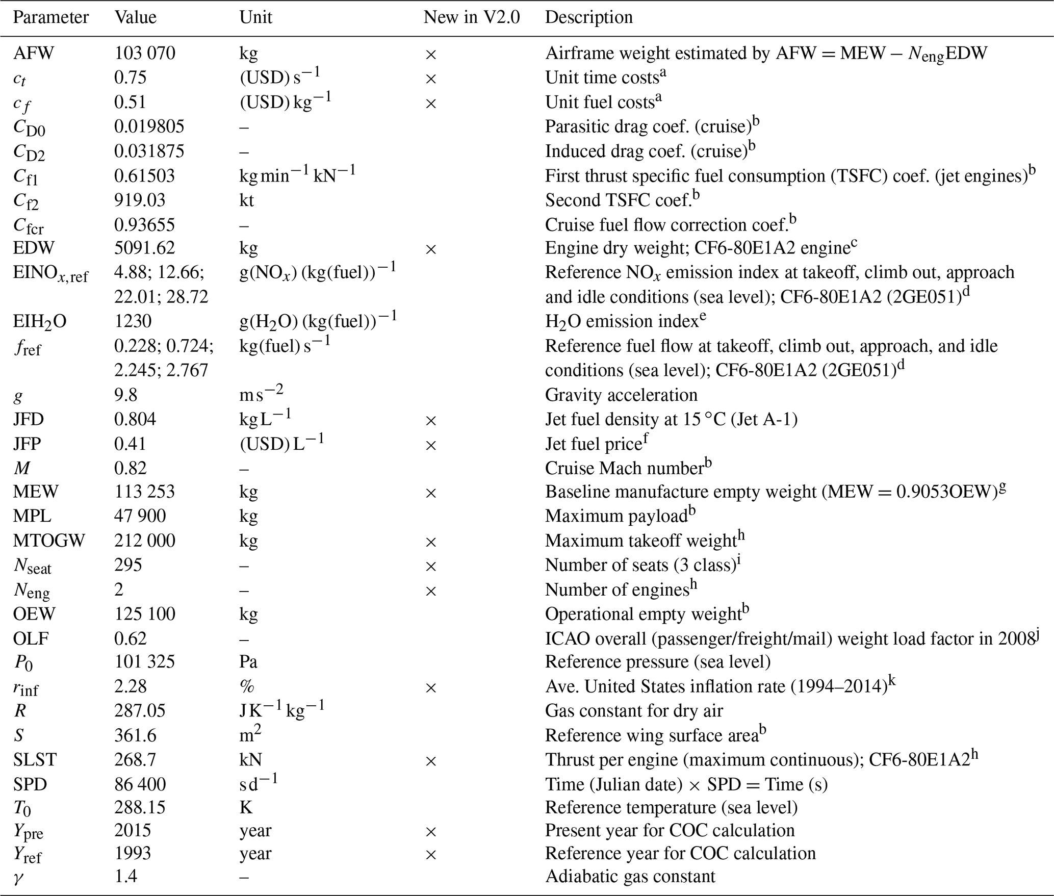
Figure 1 shows the flowchart of the submodel AirTraf 2.0. The present version is based on the model components of AirTraf 1.0, and thus this section outlines them (updates from AirTraf 1.0 are highlighted in Fig. 1). First, air traffic data and AirTraf parameters are read in the main entry point messy_initialize (Fig. 1, dark blue). They consist of a 1 d flight plan (including departure and arrival airport pairs, latitude and longitude of the airports, and departure time), EUROCONTROL's Base of Aircraft Data (BADA Revision 3.9; Eurocontrol, 2011), ICAO engine performance data (ICAO, 2005), a load factor, jet fuel price, an aircraft routing option, etc. Any arbitrary number of flight plans is applicable and is reused for AirTraf simulations longer than 2 d. Table 1 lists the relevant data of an A330-301 aircraft and constant parameters used in AirTraf 2.0 (the new parameters are listed in Table 1). Second, all the entries are distributed in parallel by the message passing interface (MPI) standard (called for the main entry point messy_init_memory; Fig. 1, blue). Third, the air traffic simulation (called the AirTraf integration; Fig. 1, light blue) is called in the main entry point messy_global_end considering local atmospheric conditions for every flight route. The AirTraf integration uses three modules: the aircraft routing module (Fig. 1, light green), the fuel–emissions–cost–climate calculation module (Fig. 1, light orange), and the flight trajectory optimization module (Fig. 1, dark green). The first module calculates flight trajectories corresponding to a selected routing option. The second module comprises a total energy model based on the BADA methodology (Eurocontrol, 2011; Schaefer, 2012) and the German Aerospace Center (DLR) fuel flow method (Deidewig et al., 1996). The third module consists of the Adaptive Range Multi-Objective Genetic Algorithm (ARMOGA version 1.2.0; Sasaki et al., 2002; Sasaki and Obayashi, 2004, 2005). Finally, simulation results are gathered from the MPI tasks. Optimum flight trajectories and global fields of flight properties (four-dimensional Gaussian grid; Fig. 1, rose red) are output. The same assumptions made in AirTraf 1.0 are applied in AirTraf 2.0; e.g., only the cruise flight phase is considered, and trajectory conflicts and operating constraints (e.g., military air space) are neglected. Further details of the model components have been reported by Yamashita et al. (2016).
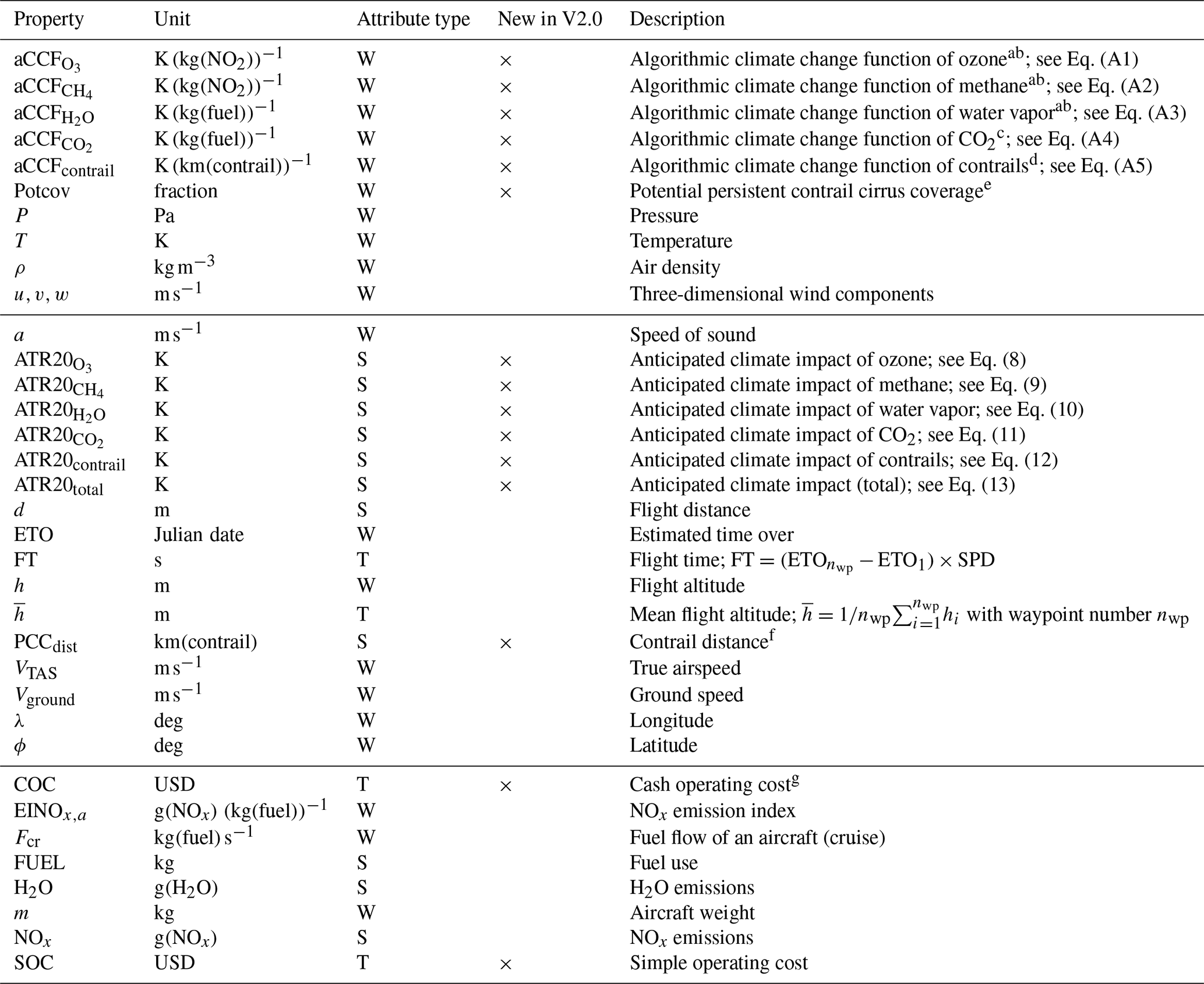
Table 2Properties assigned to a resulting flight trajectory. The properties of the three groups (divided by rows) are obtained from the nearest grid box of EMAC at the departure time of the flight, the flight trajectory calculation (Fig. 1), and the fuel–emissions–cost–climate calculation (Fig. 1; some properties are calculated in flight trajectory optimizations depending on a selected routing option). The attribute type indicates where the values of properties are allocated. “W”, “S”, and “T” stand for waypoints , flight segments , and a whole flight trajectory in column 3, respectively. The column “New in V2.0” denotes properties newly introduced in AirTraf 2.0.
a Van Manen (2017);
b Van Manen and Grewe (2019);
c Katrin Dahlmann, personal communication, 2018;
d Yin et al. (2020);
e Frömming et al. (2014);
f Yin et al. (2018a);
g Liebeck et al. (1995).
2.3 Calculation procedures of the AirTraf integration
AirTraf 2.0 follows the calculation procedures of AirTraf 1.0 described in detail in Sect. 2.4 of Yamashita et al. (2016). This section reviews the procedures of the AirTraf integration (Fig. 1, light blue) with emphasis on changes by introducing the new routing options.
A 1 d flight plan includes departure time for every flight. A flight moves to the flying process (dashed box in Fig. 1, light blue) according to the individual departure time in the time loop of EMAC. The flying process comprises four steps: flight trajectory calculation, fuel–emissions–cost–climate calculation, aircraft position calculation, and gathering global emissions (bold black boxes in Fig. 1, light blue). The first step finds an optimum flight trajectory for a selected routing option by using the aircraft routing module (Fig. 1, light green) in which the seven new routing options are introduced in AirTraf 2.0. The flight trajectory optimization module (Fig. 1, dark green) executes the flight trajectory optimization under atmospheric conditions at the departure day and time of the flight. Thus, the optimum flight trajectory varies day by day. Note that the three-dimensional wind components (u, v, w) are considered in the flight trajectory optimization for all routing options. The resulting optimum flight trajectory consists of waypoints and flight segments , where i is the index arranged from the departure (i=1) to the arrival (i=nwp) and nwp is the number of waypoints (see Fig. 3 of Yamashita et al., 2016). Table 2 lists flight properties calculated for the waypoints, the flight segments, and the whole trajectory. In AirTraf 2.0, 15 new properties are calculated, as highlighted in Table 2.
The second step, which is linked to the fuel–emissions–cost–climate calculation module (Fig. 1, light orange), calculates the flight properties of fuel, NOx emissions, COC, etc. under the atmospheric conditions (Table 2, third group). This calculation is performed once at the departure time of the flight. The methodologies of the fuel and emissions calculation module developed in AirTraf 1.0 are expanded in AirTraf 2.0. Details of the fuel–emissions calculation module and its reliability have been reported in Sects. 2.5, 2.6, and 5 of Yamashita et al. (2016).
The third step moves the aircraft to a new position along the optimum flight trajectory corresponding to the time steps of EMAC by referring to the estimated time when the aircraft passes through the waypoints (called the estimated time over, ETO; Table 2).
At the fourth step, the individual flight properties corresponding to a flight path for one time step of EMAC are gathered into the aforementioned global fields: NOx emissions, H2O emissions, fuel use, flight distance, contrail distance (PCCdist), and average temperature responses for the time horizon of 20 years (ATR20s of ozone, methane, water vapor, CO2, contrails, and total climate impact; see Sect. 2.5.7) are gathered along the flight segments (Table 2); the global fields of PCCdist and ATR20s are newly calculated by AirTraf 2.0. If the aircraft reaches the last waypoint in the time loop of EMAC, the aircraft has landed (i.e., the flight ends), and the flying process ends for this flight.
2.4 Flight trajectory optimization
The flight trajectory optimization methodologies described by Yamashita et al. (2016) are also used for the new routing options and are outlined in this section. The flight trajectory optimization module (Fig. 1, dark green) executes the optimization. The module consists of ARMOGA (version 1.2.0; Sasaki et al., 2002; Sasaki and Obayashi, 2004, 2005), which is a stochastic optimization algorithm.
A solution x (the term is synonymous with the flight trajectory) is a vector of ndv design variables: , here ndv=11. With the design variable index j , indicate latitudes and longitudes, and indicate altitudes. The jth design variable varies between lower and upper bounds . The bounds of are automatically set for a given airport pair, whereas those of are set as (flight levels; FL290 and FL410 denote 29 000 and 41 000 ft, respectively). Geographic locations of the airport pair are set according to the flight plan; altitudes of the airport pair are set to FL290. Given values of , a three-dimensional flight trajectory is represented by a B-spline curve (third-order) between the airport pair (an illustration is given in Fig. 6 of Yamashita et al., 2016).
The initial population operator (Fig. 1, dark green) generates initial values of at random within the lower and upper bounds and creates an initial “population” which represents a random set of solutions. The population size is set by np, and ARMOGA starts its search with the solutions. An evaluation function f (called an objective function) is defined depending on a selected routing option (see Sect. 2.5), and a single-objective optimization problem can be written as follows:
where no constraint function is used. The ARMOGA solves the optimization problem by the following genetic operators: evaluation, selection, crossover, and mutation (Fig. 1, dark green; Holand, 1975; Goldberg, 1989). A value of f is calculated for each of the solutions by the evaluation operator. In this study, good solutions were identified in the population by the Fonseca–Fleming Pareto ranking method (Fonseca and Fleming, 1993), the stochastic universal sampling selection (Baker, 1985) was used for the selection operator to pick two solutions (parent solutions) from the population, the Blend crossover operator (BLX-alpha; Eshelman, 1993) was applied to the parent solutions to create new solutions (child solutions), and the revised polynomial mutation operator (Deb and Agrawal, 1999) was used to add a disturbance to the child solutions. When those processes are iterated for a number of generations (the term “generation” represents one iteration of ARMOGA; this is set by ng), the population of solutions is improved by reducing f, and another superior population is created in subsequent generations. Finally, the ARMOGA finds the best solution (one optimum flight trajectory) with the minimum value of f through the whole generations; the flight properties of the solution are stored, as shown in Table 2. The flight trajectory optimization stated above is executed for every airport pair. Detailed descriptions of the optimization methodologies, appropriate ARMOGA parameter settings, and the accuracy of the optimization module have been presented in Sect. 3.2 of Yamashita et al. (2016).
2.5 Formulations of objective functions for new aircraft routing options
In AirTraf 2.0, seven new objective functions were developed for the new aircraft routing options. The following subsections describe formulations of the objective function f for those options. To calculate f, the fuel–emissions–cost–climate calculation module (Fig. 1, light orange) is used as necessary by the evaluation operator (Fig. 1, dark green) in the flight trajectory optimization.
2.5.1 Fuel use
The objective function for the fuel option represents the sum of fuel use – kg(fuel) – of a flight:
where FUELi is the fuel use of the ith flight segment (Table 2).
2.5.2 NOx emissions
The objective function for the NOx option represents the sum of NOx emissions – g(NOx) – of a flight:
where NOx,i is the NOx emissions of the ith flight segment; is the NOx emission index under actual flight conditions at the ith waypoint (Table 2) and is calculated using the ICAO engine performance data (ICAO, 2005; see Sect. 2.6 of Yamashita et al., 2016).
2.5.3 H2O emissions
The objective function for the H2O option represents the sum of H2O emissions – g(H2O) – of a flight:
where H2Oi is the H2O emissions of the ith flight segment (Table 2); EIH2O is the emission index of H2O and was set as EIH2O=1230 g(H2O)(kg(fuel))−1 (Table 1). The H2O emissions are proportional to the fuel use by assuming an ideal combustion of jet fuel. Thus, this option yields the same results as the fuel option in AirTraf 2.0. If an alternative fuel option is introduced, the H2O option probably differs from the fuel option because the emission index may not be constant.
2.5.4 Contrail formation
Yin et al. (2018a) developed the routing option to avoid contrail formations by using the submodel CONTRAIL (version 1.0; Frömming et al., 2014) which calculates the potential persistent contrail cirrus coverage Potcov (Ponater et al., 2002; Burkhardt et al., 2008; Burkhardt and Kärcher, 2009; Grewe et al., 2014b) within an EMAC grid box. The Potcov represents the fraction of the grid box which can be maximally covered by contrails under the simulated atmospheric condition. The threshold for contrail formation is determined from a parameterization scheme based on the thermodynamic theory of contrails, i.e., the Schmidt–Appleman theory (Schmidt, 1941; Appleman, 1953; Schumann, 1996). In the CONTRAIL submodel, Potcov indicates the difference between the maximum possible coverage of both contrails and cirrus and the coverage of natural cirrus alone; values of Potcov along the waypoints are taken from the nearest grid box (Table 2). With that, we define a contrail distance (PCCdist) – in km(contrail) – as Potcov multiplied by the flight distance in kilometers. The corresponding routing option minimizes the total contrail distance of a flight, and thus the objective function is formulated as follows:
where PCCdist,i is the contrail distance of the ith flight segment, Potcovi is the potential persistent contrail cirrus coverage at the ith waypoint, and di is the flight distance of the ith flight segment (Table 2). Note that the objective function is formulated in the simple form to consider only the contrail distance. Thus, further physical processes such as contrail spreading, changes in contrail coverage area, contrail lifetime, and the contrail radiative forcing are not included.
2.5.5 Simple operating cost (SOC)
The cost index (CI) is set during a real flight to manage airline operation costs and is defined as the ratio of time cost to fuel cost (). A low CI value causes an aircraft to minimize fuel use with a sacrifice of flight time, which enables a long-range flight. Conversely, a high CI value causes the aircraft to minimize flight time with extra fuel use. Generally, the operating costs are a function of flight time and fuel. Thus, the minimum cost solution lies in a trade-off between flight time and fuel (Cook et al., 2009; Marla et al., 2016). Here the objective function simply represents the sum of the time and the fuel costs on the basis of the CI features:
where ct and cf are the unit costs of time and fuel, respectively (Table 1), and Vground,i is the ground speed at the ith waypoint (Table 2). Note that the ct includes the cost elements for flight crew, cabin crew, and maintenance for both airframe and engines.
2.5.6 Cash operating cost (COC)
The COC is a comprehensive economic criterion for evaluating airline operation costs (Liebeck et al., 1995). The COC includes the cost elements for flight crew, cabin crew, landing fee, navigation fee, fuel, and maintenance for both airframe and engines (no costs for depreciation, insurance, and interest are included). The COC calculation method for international flights (Liebeck et al., 1995) was employed. Those cost elements were calculated on the basis of the price in 1993 and were scaled to 2015 by the average United States inflation rate of average consumer prices rinf (Table 1; IMF, 2016). Only the fuel cost was directly calculated with the current jet fuel price (JFP) (Table 1; IATA, 2017). A block time and a block fuel originally used in the method were replaced by the total flight time (FT) and the fuel use of in AirTraf 2.0, respectively (Table 2). The objective function can be written as follows:
where C denotes a cost. A detailed description of the COC calculation method has been reported in Liebeck et al. (1995). Given the parameters and variables listed in Tables 1 and 2, Eq. (7) becomes a function of the flight time and the fuel.
2.5.7 Climate impact
The climate-optimized routing was carried out by using the aCCFs (Van Manen, 2017; Yin et al., 2018b, 2020; Van Manen and Grewe, 2019) calculated by the submodel ACCF. The aCCFs are approximation functions based on regression analyses for the CCF data set which was obtained from detailed EMAC model simulations including radiative impacts (see Sect. 1); the CCF data set for contrails was exceptionally obtained from contrail RF calculations based on the European Centre for Medium-Range Weather Forecasts (ECMWF) Re-Analysis Interim (ERA-Interim) data (Dee et al., 2011) and contrail trajectory data (Yin et al., 2020; the definition of the aCCFs is provided in the Appendix, and examples are shown in Fig. S1 in the Supplement). The aCCFs represent a correlation of meteorological variables at the time of flight with anticipated climate impacts; i.e., ATR20s of ozone, methane, water vapor, CO2, and contrails are estimated on a per unit basis by
where the respective aCCF values of ozone, methane, water vapor, CO2, and contrails are given as flight properties at the ith waypoint. These five ATR20s are calculated for flight segments (Table 2) and are combined into an objective function to represent an anticipated climate impact of a flight (in K):
where ATR20contrail,i can take positive and negative values because the aCCFcontrail consists of two formulas for the daytime and nighttime contrail effects (see Eq. A5 in the Appendix). We acknowledge the large uncertainties in the global temperature response especially from contrails (ATR20contrail) due to uncertainties in the efficacy of the contrail forcing (Hansen et al., 2005; Ponater et al., 2005). In addition, the aCCFs are derived based on the CCF data of the North Atlantic region and are applicable to the northern and high latitudes. Further details of the aCCFs have been reported in the literature mentioned above.
3.1 Simulation setup
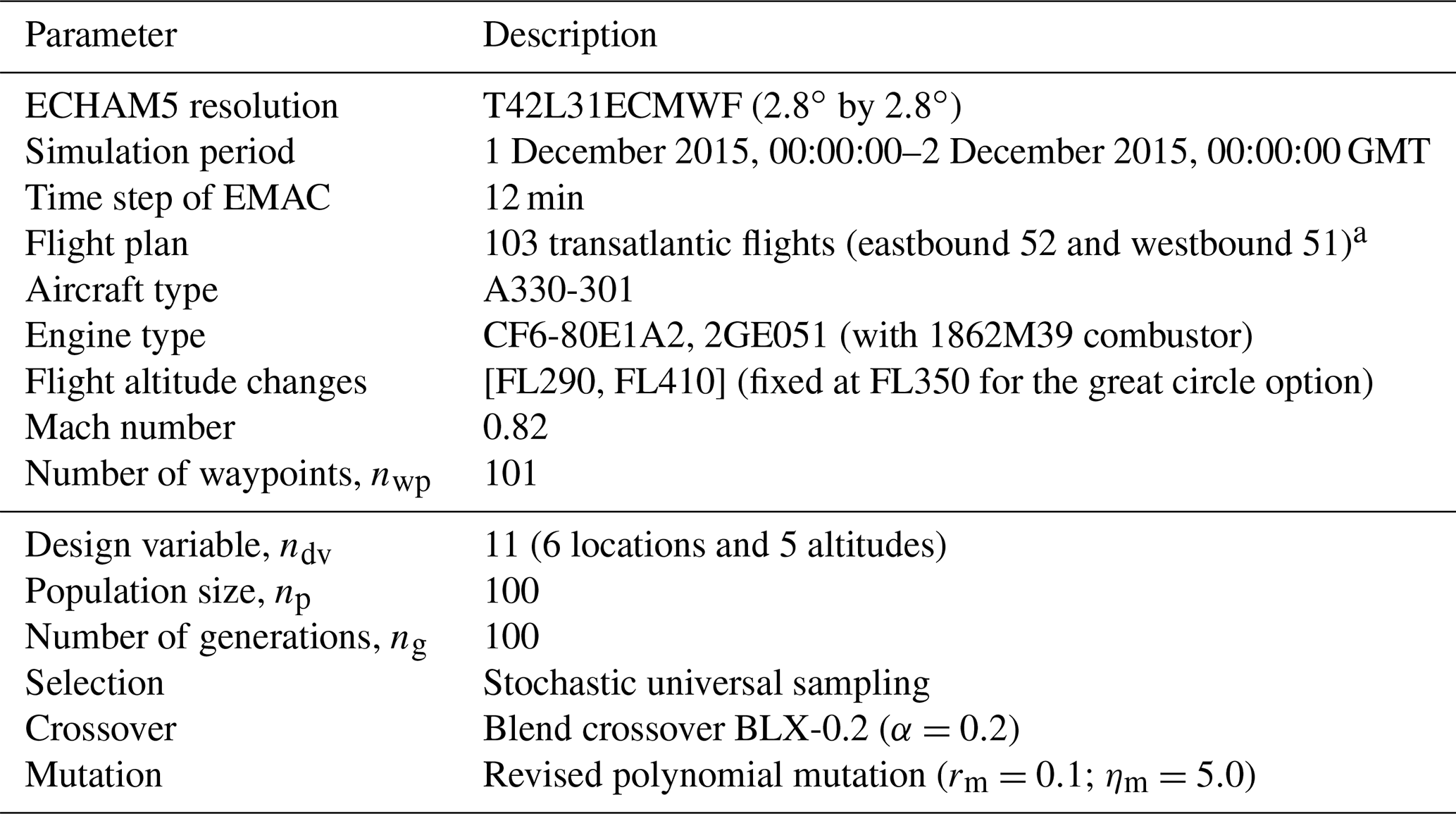
Table 3Setup for AirTraf 1 d simulations. The setups of the two groups (divided by rows) are used for AirTraf/EMAC and for ARMOGA (Sasaki et al., 2002; Sasaki and Obayashi, 2004, 2005). The user-specified crossover parameter is α, rm is a mutation rate, and ηm is a parameter controlling the shape of a probability distribution. Details of these parameters are described in Yamashita et al. (2016).
a Grewe et al. (2014a) and REACT4C (2014).
Nine 1 d simulations were carried out for a demonstration of AirTraf 2.0. Table 3 lists the simulation setups. The same setups that we used for the consistency check for AirTraf 1.0 simulations (Yamashita et al., 2016) were employed; only the simulation period was changed to a recent day which showed a typical weather condition in winter with a strong jet stream (see Fig. S2 in the Supplement). The flight altitude for the great circle option was set to FL350; the altitude for the other options was calculated in the trajectory optimization within [FL290, FL410], as mentioned in Sect. 2.4. The transatlantic flight plan (103 flights) of an Airbus A330 aircraft was provided by Grewe et al. (2014a) and REACT4C (2014). The setups for the optimization parameters were determined by the benchmark tests (Yamashita et al., 2016).
3.2 Optimized flight trajectories and global fields
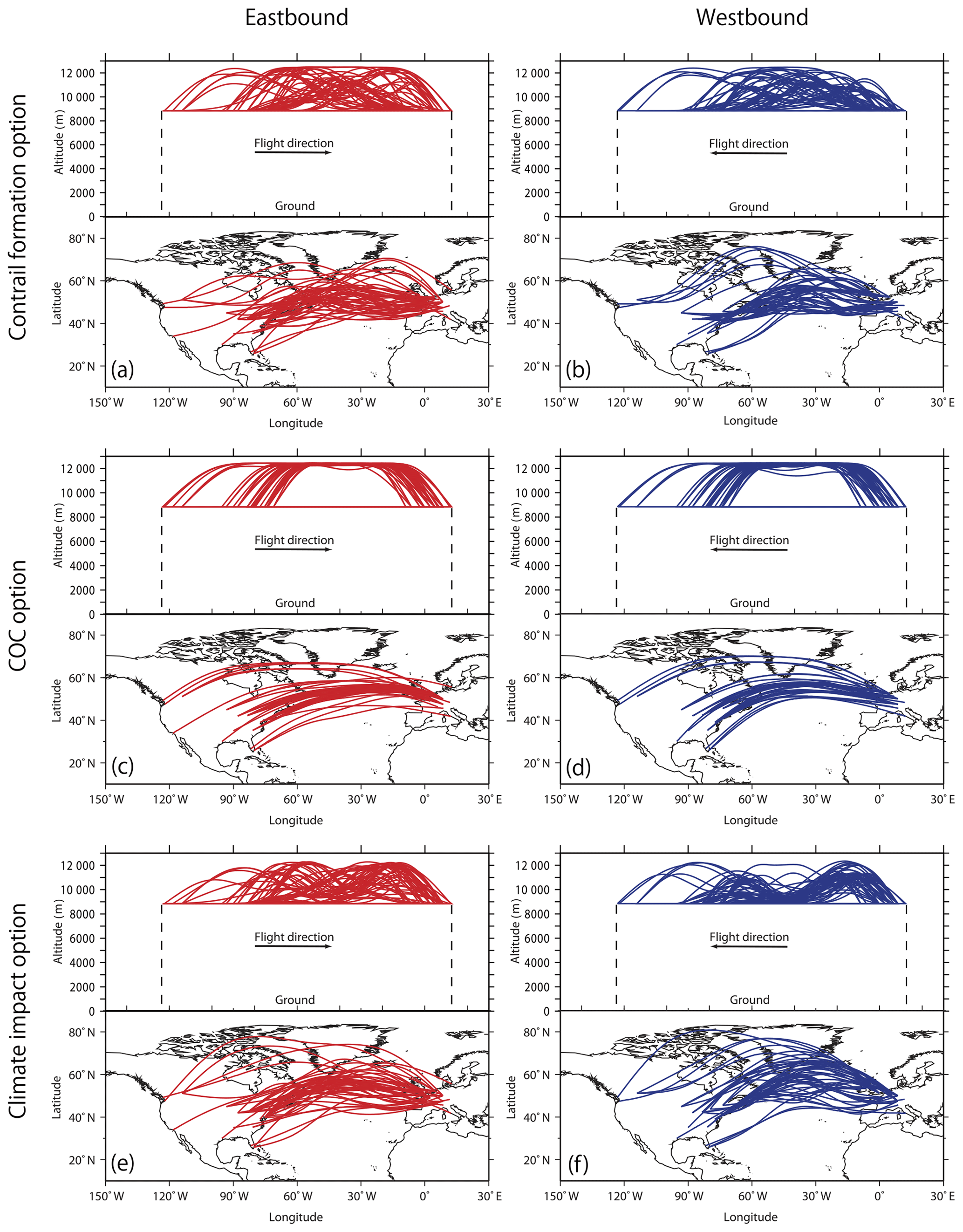
Figure 2Optimized flight trajectories from a 1 d AirTraf simulation (52 eastbound and 51 westbound flights) for the contrail formation (a, b), the COC (c, d), and the climate impact routing options (e, f). For each figure, the trajectories are shown in the vertical cross section (top) and projected on the ground (bottom).
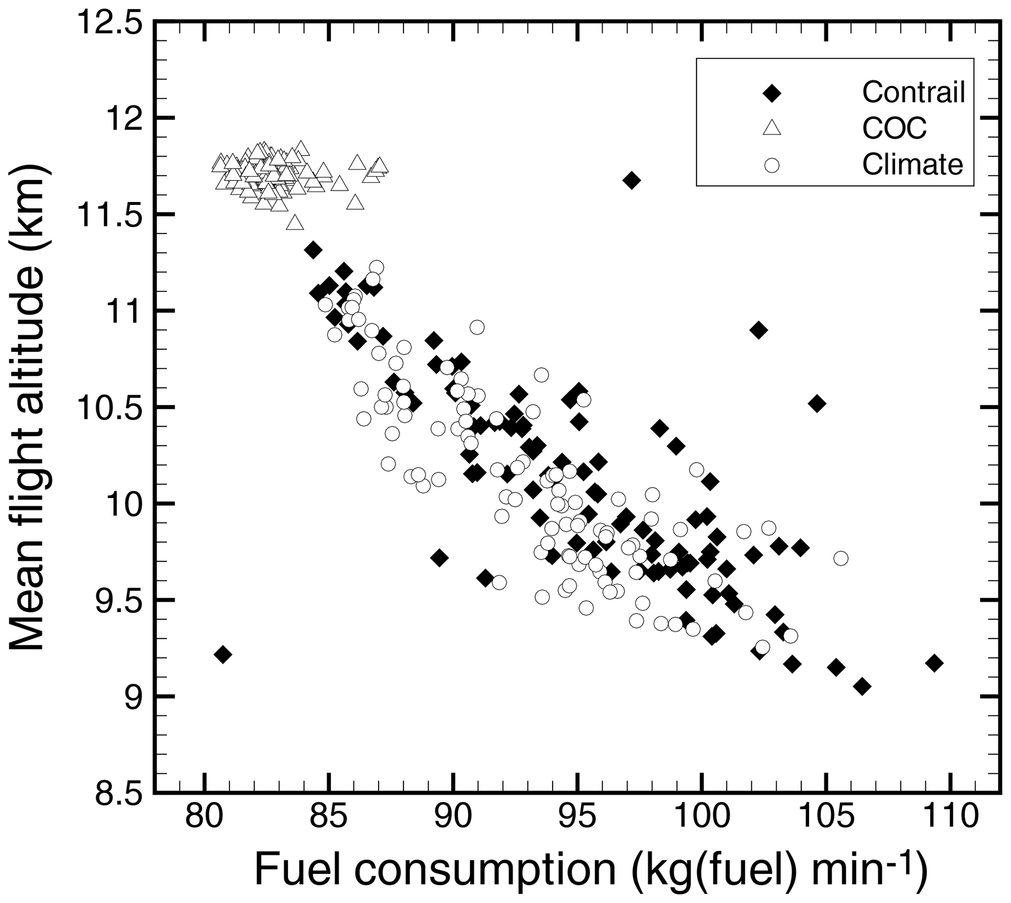
Figure 3Mean fuel consumption vs. mean flight altitude for 103 individual flights obtained by the contrail formation, the COC and the climate impact routing options.
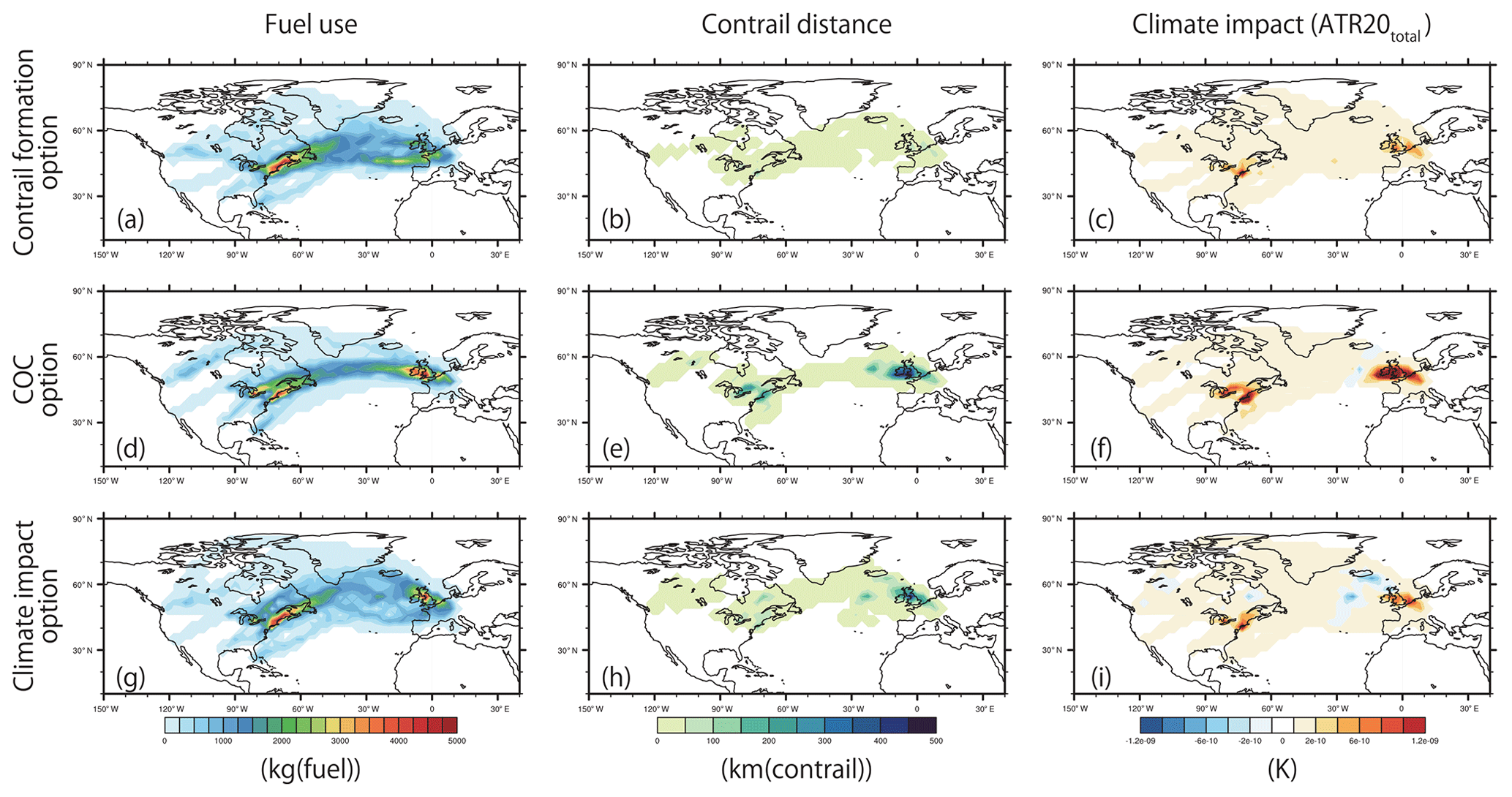
Figure 4Vertically integrated distribution of fuel use, contrail distance, and climate impact indicated by ATR20total during the day (from 1 December 2015, 00:00:00 to 1 December 2015, 00:00:00 GMT). (a–c) Contrail formation option. (d–f) COC option. (g–i) Climate impact option. These distributions were obtained with the optimized flight trajectories shown in Fig. 2 (sum of 103 flights).
To display typical simulation outputs, the obtained optimized trajectories and global fields for the contrail, the COC, and the climate options are shown. Figure 2 shows the optimized trajectories for those options (optimized trajectories for other options are shown in Supplement Fig. S3). Obviously, the optimum trajectories vary with the routing options. Figure 2c and d show that the COC optimum trajectories of the eastbound flights leap up over the North Atlantic Ocean, whereas the trajectories of the westbound flights are shifted northward. As the jet stream is located at around 40∘ N and 50∘ W (see Fig. S2 in the Supplement), the eastbound trajectories are optimized to benefit from tailwinds of the jet stream and the westbound trajectories avoid headwinds of the jet stream by detouring northward. In addition, most of those trajectories are located at high flight altitudes (∼FL410, 12.5 km). Figure 3 shows the mean fuel consumption – in kg(fuel) min−1 – vs. mean flight altitude (in km) for individual flights for the three routing options. Because fuel consumption decreases as a result of aerodynamic drag reduction at high altitudes (Fichter et al., 2005; Schumann et al., 2011; Yamashita et al., 2016), the COC optimum trajectories select the high flight altitudes, as shown in Fig. 3. We acknowledge that limitations of BADA 3 affect the selection of the flight altitudes (the same applies to the fuel, the NOx, the H2O, and the SOC options; see Fig. S3 in the Supplement). According to Nuic et al. (2010), BADA 3 has a tendency to underestimate aircraft fuel consumption at high altitudes and Mach numbers as the compressibility effect and wave drag are not modeled. These effects will cause differences in the selection of the flight altitudes. In contrast, the contrail and the climate options show complex-shaped trajectories with various flight altitude changes (see Fig. 2a, b, e, and f).
The global fields of fuel use, contrail distance, and climate impact indicated by ATR20total for the three options are shown in Fig. 4, in which distributions represent the sum of all the flights during the day. We see from Fig. 4b, e, and h that the contrail option certainly decreases the contrail formation, which is mostly located over northwest Europe and over the east coast of the United States. A comparison of Fig. 4a, d, and g shows that the COC option produces a narrower fuel distribution than that of the contrail and climate options. In addition, Fig. 4c, f and i show that the climate option decreases the positive values of ATR20total (warming effects) over northwest Europe and over the east coast of the United States and produces regionally negative values (cooling effects) near Iceland and over eastern Canada, which result in the net climate impact reduction. A comprehensive analysis of the optimized trajectories for the calculated fields is beyond the scope of this paper. However, it is apparent from Fig. 4 that the optimized trajectories successfully decrease the respective objects (target measures) which should be minimized (this point is discussed quantitatively in Sect. 3.3).
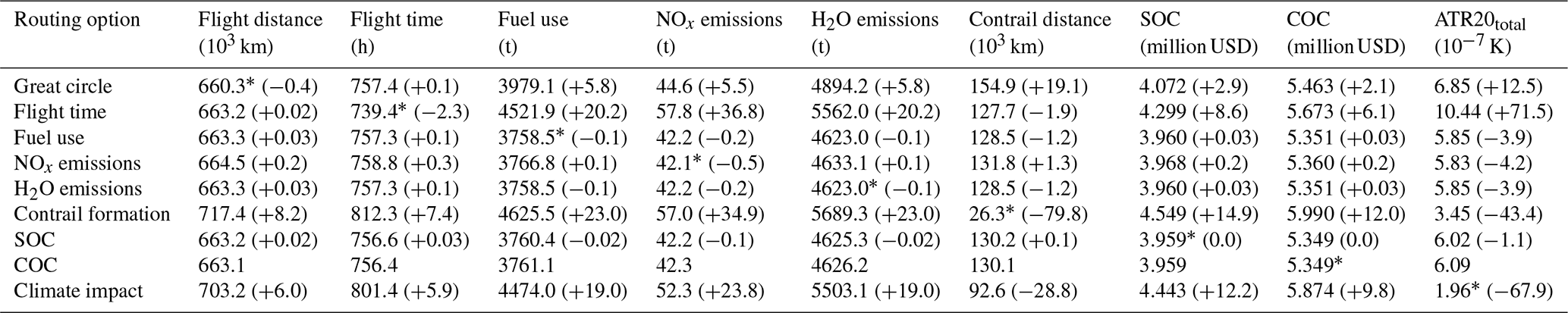
Table 4The nine performance measures obtained from the 1 d AirTraf simulations with different aircraft routing options (the values indicate the sum of 103 flights). The minimum values of each performance measure are marked with an asterisk; changes (in %) relative to the COC option are given in parentheses. Bar charts of the same data are given in Fig. S4 in the Supplement.
3.3 Characteristics of aircraft routing options
To examine the characteristics of the routing options, Table 4 lists a summary of nine performance measures of the 1 d air traffic (total 103 flights) for specific routing options (bar charts are given in Supplement Fig. S4). Relative changes (in %) to the COC option are also listed in Table 4, considering this option as a reference (the COC option is assumed to be the current aircraft routing strategy). Table 4 shows that individual options successfully minimize their own object (target measure; see measures marked with an asterisk in Table 4). These results confirm that the new routing options work correctly in AirTraf 2.0 since we solve a single-objective minimization problem defined by Eq. (1) for each routing option.
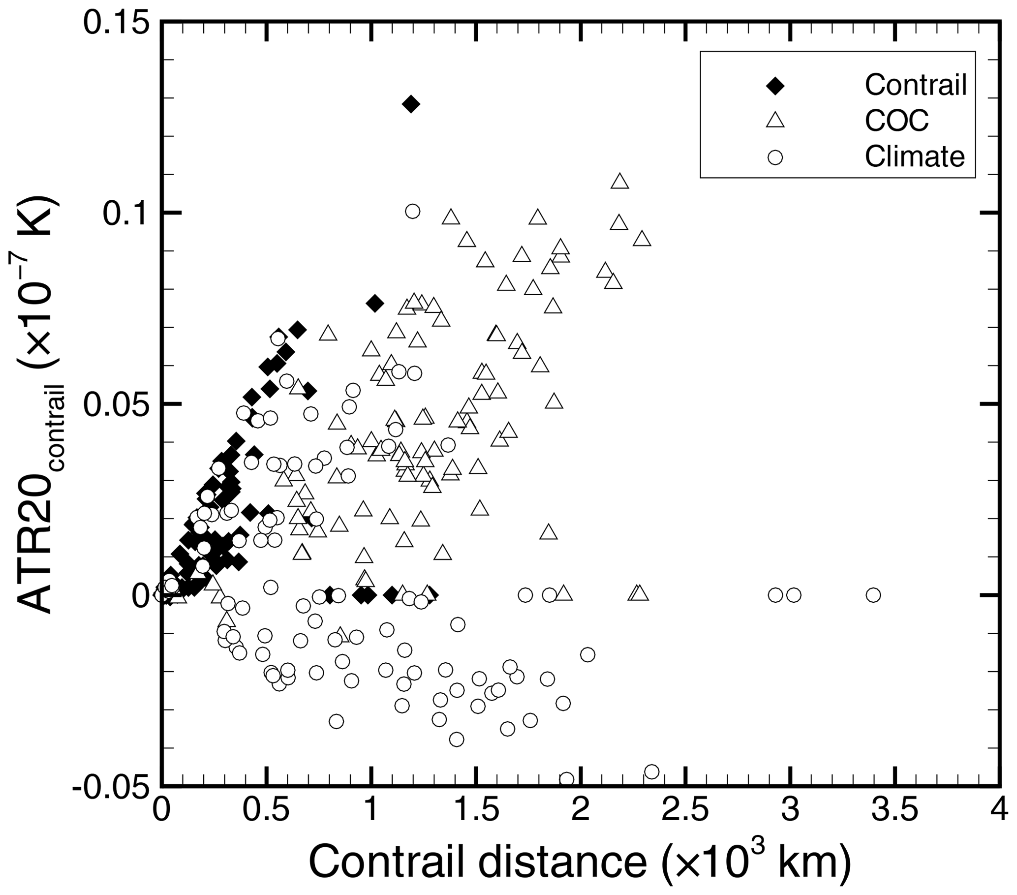
Figure 5Contrail distance vs. ATR20contrail for 103 individual flights obtained by the contrail formation, the COC, and the climate impact routing options.
The individual routing options are now discussed in turn. We see from Table 4 that the great circle option has the minimum flight distance of 660.3×10³ km, whereas this option increases the other measures. The time option shows the minimum flight time of 739.4 h with a large penalty on fuel use, NOx emissions, H2O emissions, SOC, COC, and ATR20total (further discussion in Sect. 4). The fuel option shows the minimum fuel use of 3758.5 t. Of the nine routing options, the fuel (and also the H2O), the NOx, the SOC, and the COC options obtain similar values on all the measures (see also Supplement Fig. S4); these options show decreased fuel use, NOx and H2O emissions, SOC, and COC, whereas contrail distance and ATR20total increase. The difference among these options is considered significant for airline operations and thus is discussed in more detail in Sect. 4. The contrail option shows the minimum contrail distance of 26.3 × 10³ km and the second-lowest ATR20total of K, whereas the other measures increase considerably. This option allows aircraft to widely detour the potential contrail regions (because no constraint function is used in Eqs. 1 and 5; see below for more discussion). Thus, the flight distance, the flight time, and the fuel use increase drastically, which results in the increase of NOx and H2O emissions, SOC, and COC. In particular, the contrail option shows the highest COC of 5.99 million USD of the nine routing options. Comparing the contrail option with the COC option indicates that the contrail distance decreases with an additional fuel use of 8.3 kg(fuel)(km(contrail))−1, i.e., the additional COC of 6.20 USD(km(contrail))−1. The SOC and the COC options are comparable. The two options show similar values for all the measures and have the same minimum SOC of 3.96 million USD and COC of 5.35 million USD. In fact, the obtained optimum trajectories for those options are approximately the same (see Fig. 2c, d and Supplement Fig. S3k, l). This is because the objective function of the two options is a function of flight time and fuel, as defined in Eqs. (6) and (7). An interesting aspect of their performance measures is that both options do not correspond to the minimum flight time and fuel use (see further discussion in Sect. 4). The climate option achieves the minimum ATR20total of K and shows the second-shortest contrail distance of 92.6×10³ km, whereas the other measures increase; this option in particular shows the second-highest COC of 5.87 million USD. The present results indicate that the contrail and the climate options considerably reduce the climate impact indicated by ATR20total; however, these options increase COC. The cost–benefit performance (i.e., the COC increment per ATR20total reduction) for the contrail and the climate options are 0.24 and 0.13 , respectively. Thus, the climate option seems to be a more cost-effective option. Note that this performance is a narrow result obtained using AirTraf 2.0 under specific conditions (e.g., the simulations were carried out with the 103 North Atlantic flights on 1 December 2015, as shown in Table 3). Figure 5 shows the contrail distance (in 103 km) vs. ATR20contrail (in 10−7 K) for individual flights for the contrail, the COC, and the climate options. We see that the contrail option decreases the contrail distance drastically and shows the positive values of ATR20contrail for almost all the flights. On the other hand, the climate option has longer contrail distances than those of the contrail option (although the climate option achieves the second-shortest total contrail distance, as shown in Table 4) and shows the negative values of ATR20contrail for many flights. These results imply that the contrail option minimizes the overall contrail distance at all times, whereas the climate option actively forms cooling contrails during the day and avoids the formation of warming contrails during the day and night. Finally, we believe that the climate benefits described above are most likely an upper limit because airspace congestion and air traffic management could reduce the flexibility for flights to perform these trajectory optimizations.
This paper presents the extended version of the submodel AirTraf which offers additional aircraft routing options for defining overall target functions for the flight trajectory optimization. To confirm the consistency of AirTraf simulations, the relative changes in the performance measures among the routing options (listed in Table 4 in parentheses) are compared with previous studies. The quantitative values of the changes in the performance measures vary depending on different methodologies, atmospheric conditions, simulation periods, flight plans, aircraft/engine types, cost/climate impact metrics, etc. Thus, a direct comparison in magnitude of our results with published studies is difficult; the sign of the relative changes in the measures is compared. Note that the great circle and the time options have been verified before (Yamashita et al., 2016). In addition, the H2O option yields the same results as the fuel option (see Sect. 2.5.3 and Table 4); the SOC option is comparable to the COC option (see Sect. 3.3 and Table 4). Thus, we omit any discussion of the H2O and the SOC options here.
First, the time, the fuel, and the COC options are analyzed. As defined in Sect. 2.5.6, COC is a combined function of flight time and fuel. To minimize COC, one may attempt to reduce both factors simultaneously; however, a trade-off between the flight time and the fuel generally exists. Table 4 shows that the time penalty of flying minimum fuel trajectories is 2.4 percentage points, whereas the fuel penalty of flying minimum time trajectories is 20.3 percentage points. A similar trade-off was reported by two published studies. Celis et al. (2014) addressed a single-objective flight trajectory optimization on total flight time and fuel use under ISA conditions. A typical single-aisle aircraft (150 passengers) with twin turbofan engines was assumed; the aircraft speed and the flight altitude in eight flight segments were optimized for a given flight trajectory (a quasi-full flight profile optimization). Compared to the minimum time trajectory, the fuel optimum trajectory decreased the fuel use by 31.7 percentage points with an increased flight time of 14.0 percentage points. Rosenow and Fricke (2016) compared performances for the minimum time and the minimum fuel trajectories for a flight from Frankfurt (Main) to Dubai for a Boeing B777 freighter on 2 February 2016 at 12:00 GMT. The comparison showed that the fuel optimum trajectory decreased fuel use by 8.0 % with an increased flight time of 3.7 %. These studies imply that the minimum COC solution lies between the minimum time and the minimum fuel solutions. In fact, Table 4 shows that the COC option has more flight time than that of the time option and that the COC option consumes more fuel than that of the fuel option. The COC option yields the values of compromise (i.e., not minimum) of flight time and fuel. Nonetheless, this option achieves the minimum COC. The submodel AirTraf 2.0 can consistently differentiate those three solutions.
To support the discussion above, the fuel and the COC options are compared in detail. Erzberger and Lee (1980) compared the minimum fuel and the minimum direct operating cost (DOC) trajectories for a short-haul route for a Boeing 727-100 aircraft on the basis of optimum control theory (Bryson and Ho, 1969) under United States standard atmospheric conditions. They showed that flying “minimum fuel” reduced fuel use by 6.9 %, whereas the time and the DOC penalties of the trajectory were 23 % and 6 %, respectively (constrained thrust case). Our results in Table 4 show that the fuel option reduces fuel use by 0.1 %, whereas the time and the COC penalties of the option are 0.1 % and 0.03 % compared to those measures of the COC option. The signs of these relative changes obtained from our results agree with those shown by Erzberger and Lee (1980). In addition, the time and the COC options are compared in a perspective of airline operating economics. Although the time option increases fuel use, NOx emissions, H2O emissions, SOC, COC, and ATR20total (fuel use and COC increase by 20.2 % and by 6.1 %, respectively), the option decreases flight time by 2.3 % compared to that of the COC option. In other words, the time option reduces flight time with the extra cost of 19 034.74 USD h−1 (=269.66 EUR min−1, converted as 1 USD=0.85 EUR on 18 September 2018; European Central Bank, 2018). In a context of delay recovery, this extra cost is the same order of magnitude to flight delay costs. If the flight delay costs exceed the extra cost due to the time option, operators would determine to fly faster by using the time option to recover the delay. Cook et al. (2004, 2009) reported that the flight delay costs, which are associated with delayed passengers, additional fuel use, flight crew, cabin crew, and marginal maintenance costs, reached several hundred Euros per minute. The extra cost calculated from our results agrees well with this report.
Compared to the COC option, the NOx option decreases the NOx emissions by 0.5 %, leading to a COC increase of 0.2 %. Mulder and Ruijgrok (2008) analyzed the effects of varying cruise conditions on NOx emissions and on DOC from the cruise NOx simulation model (Bremmers, 1999) by assuming a cruise range of 5800 km with a Boeing 747-400 aircraft under ISA conditions. They clearly concluded that a reduction of NOx emissions caused a cost increase. Our results agree well with this conclusion. Moreover, the NOx option differs from the fuel option because the amount of NOx emissions depends not only on fuel use but also on the NOx emission index, as defined in Eq. (3). The emission index depends strongly on the ambient atmospheric conditions at every waypoint (see Sect. 2.6 of Yamashita et al., 2016). Table 4 shows that the NOx option decreases the NOx emissions by 0.3 percentage points, whereas this option increases flight time by 0.2 percentage points and fuel use by 0.2 percentage points compared to those measures of the fuel option. Celis et al. (2014) addressed a single-objective flight trajectory optimization on total fuel use and on NOx emissions with the same simulation setup described above. Compared to the minimum fuel trajectory, the minimum NOx trajectory decreased NOx emissions by 10.4 percentage points, whereas the trajectory increased time by 1.0 percentage point and fuel use by 3.9 percentage points. The signs of the relative changes obtained from our results are in good agreement with those shown by Celis et al. (2014).
The contrail option drastically decreases contrail distance by 79.8 % and ATR20total by 43.4 %, whereas this option increases fuel use by 23.0 % and COC by 12.0 % compared to those measures of the COC option. The contrail option is effective in order to reduce the climate impact, as pointed out by previous studies introduced in Sect. 1. Here those relative changes in the measures are compared with two published studies. Rosenow et al. (2017) performed a 1 d European air traffic optimization on 25 July 2016. The total number of 13 584 flights over Europe (containing 16 aircraft types) was employed; their three-dimensional flight profiles were optimized for airline costs (termed as the cost performance indicators, CPI) and environmental impacts (termed as the ecological performance indicators, EPI). They revealed that an additional contrail avoidance intent decreased contrail costs by 31.5 % (contrail formations were converted into a monetary value) and EPI by 5.2 %, whereas the intent increased fuel use by 0.05 % and CPI by 0.5 % over those of the minimum cost strategy. The signs of the relative changes obtained from our simulations are consistent with those shown by Rosenow et al. (2017). Furthermore, Sridhar et al. (2013) applied a contrail reducing strategy to aircraft flying between 12 airport pairs (287 flights) in the United States on 12 April 2010. The three-dimensional contrail reducing strategy showed a trade-off between contrail formation time (time spent in traveling through contrail formation regions) and fuel consumption. Representative points on the trade-off curve showed that the contrail formation time decreased by 4415 and by 5301 min with an additional fuel use of 20 000 and of 131 000 kg(fuel), respectively, over those of a wind-optimal strategy (this strategy is regarded as an economically optimal strategy; see Sect. 2.4 of Yamashita et al., 2016). This study clearly indicated the fuel increase by avoiding contrail formations. Our results agree well with the finding of Sridhar et al. (2013).
Table 4 clearly shows a trade-off between economic cost and climate impact (see also Supplement Fig. S4). Compared to the COC option, the climate option decreases ATR20total by 67.9 % with an additional COC of 9.8 %. A similar trade-off certainly exists between the minimum COC and the minimum climate impact trajectories for each airport pair. The trade-off obtained from our results agrees with that indicated by many studies (see Sect. 1). Moreover, Niklaß et al. (2017) performed an aircraft trajectory optimization for nine North Atlantic flight routes varying weighting factors on average temperature response over 100 years (ATR100) and on COC under ISA conditions. They showed a clear trade-off between the cost and the climate impact. The minimum climate impact trajectories, on average, reduced ATR100 by 28.4 % with an additional COC of 7.1 % compared to those measures of the minimum COC trajectories. Our results agree with those shown by Niklaß et al. (2017). As discussed above, many previous studies corroborate the consistency of the AirTraf simulations.
We introduced updates to the air traffic simulation model AirTraf in the chemistry–climate model EMAC. The submodel AirTraf 2.0 was developed according to the MESSy standard and was described in detail in this paper. This submodel introduces seven new aircraft routing options for air traffic simulations: the fuel use, the NOx emissions, the H2O emissions, the contrail formation, the simple operating cost, the cash operating cost, and the climate impact options. Our flight trajectory optimization methodology consists of genetic algorithms; the methodology was similarly used and was validated beforehand (Yamashita et al., 2016). The particular strength of AirTraf is to enable a flight trajectory optimization for a global flight movement set in the atmosphere which is comprehensively described by EMAC. The novel routing option, i.e., the climate impact option, has been integrated in AirTraf 2.0. This option uses meteorological variables in terms of (spatially and temporally varying) aviation climate impact estimated by the aCCFs, and optimizes flight trajectories by minimizing their anticipated climate impact. As the aCCFs are new proxies for the climate-optimized routing, AirTraf takes a role in verifying the aCCFs themselves and the climate impact option based on the aCCFs in multi-annual (long-term) simulations.
To test the submodel AirTraf 2.0, example simulations were carried out with 103 North Atlantic flights of an Airbus A330 aircraft for a typical winter day. AirTraf 2.0 simulates the 1 d air traffic successfully for the newly developed routing option concerning different optimization objectives, e.g., contrail avoidance, cash operating cost, and climate impact (represented by average temperature response over 20 years) and finds the different families of optimum flight trajectories which minimize the corresponding objective functions. The characteristics of these routing options include that aircraft are flown as the minimum economic cost with both the SOC and the COC options. These options are comparably effective for economic cost indices. AirTraf 2.0 differentiates the minimum time, the minimum fuel, and the minimum COC options. The COC option lies between the minimum time and the minimum fuel options and thus minimizes COC by taking the best compromise between the flight time and the fuel use into account. The NOx option minimizes NOx emissions; this option differs from the fuel and the COC options. The contrail and the climate options decrease the climate impact (indicated by ATR20total), which causes extra operating costs. A trade-off between the cost and the climate impact certainly exists. Compared to the COC option, the climate and the contrail options decrease ATR20total by 67.9 % and by 43.4 % with an increase of COC of 9.8 % and of 12.0 %, respectively. Thus, the climate option seems to be more effective on the cost–benefit performance than the contrail option. We believe that these climate benefits are most likely an upper limit. The simulation results were compared with literature data. The relative changes in the performance measures among the various routing options agree well with those shown by many previous studies. This comparison has limitations because of different methodologies, different atmospheric conditions, etc. Nonetheless, a lot of literature data offer evidence to indicate the consistency of the AirTraf simulations.
The integration of AirTraf into EMAC allows one to optimize flight trajectories and to study aircraft routings under historical, present-day, and future conditions of the climate system. We acknowledge that the simulation results depend on the atmospheric conditions of the target day. Thus, it is important to examine whether the findings, e.g., the trade-off between the cost and the climate impact, are common under any atmospheric conditions. Recently, Yamashita et al. (2020) examined this for representative weather types over the North Atlantic by using EMAC with AirTraf 2.0. Furthermore, the integrated aircraft routing options could be extended to conflicting scenarios. Yin et al. (2018a) investigated a trade-off between flight time and contrail formation for transatlantic flights by combining the time and the contrail options. Another option could easily be created by adding a corresponding objective function. The AirTraf development presented in this paper leads to a further detailed understanding of characteristics of various aircraft routing strategies.
The aCCFs are calculated by the submodel ACCF (version 1.0). The derivation and validation of the aCCFs of ozone, methane, and water vapor have been published by Van Manen (2017), Yin et al. (2018b), and Van Manen and Grewe (2019); the aCCF of contrails is described by Yin et al. (2020). The aCCFs for ozone, methane, water vapor, CO2, and contrails are formulated as follows:
where T is the atmospheric temperature (in K), Φ is the geopotential (in m2 s−2), Fin is the incoming solar radiation at the top of atmosphere (in W m−2), PV is the potential vorticity (in PVU; ), and OLR is the outgoing longwave radiation (in W m−2). Given values of these meteorological variables, Eqs. (A1) and (A2) yield and (in K(kg(NO2))−1), Eqs. (A3) and (A4) yield and (in K(kg(fuel))−1), and Eq. (A5) yields aCCFcontrail (in K(km(contrail))−1). The is the sole constant value (K. Dahlmann: Personal communication, 2018). The is calculated by using the nonlinear climate–chemistry response model AirClim (Grewe and Stenke, 2008; Dahlmann, 2012; Dahlmann et al., 2016) assuming a 1 Tg fuel use in 2010 with the annual growth rate according to the future global aircraft scenario Fa1 (Penner et al., 1999). The is the averaged temperature response of CO2 for the period 2010–2029 (in K per kilogram of fuel) calculated by AirClim. The aCCFcontrail for the nighttime contrails takes positive values; if the temperature is less than 201 K, aCCFcontrail for the nighttime contrails is set to 0. The aCCFcontrail for the daytime contrails can take positive and negative values depending on the OLR (the threshold is −193.18 W m−2). As for the time boundaries of day and night, the local time and solar zenith angle are calculated for locations where contrails could form (Potcov>0). For locations in darkness, the time of sunrise is then calculated. If the time between the local time and sunrise is greater than 6 h, the aCCFcontrail for the nighttime contrails is applied. If the contrail forms in daylight, or in darkness but with less than 6 hours before sunrise, the aCCFcontrail for the daytime contrails is applied. These calculations are performed online in EMAC by the submodel ACCF. In AirTraf 2.0, those five aCCFs are calculated as flight properties for waypoints, and then the corresponding ATR20s are calculated for flight segments (see Table 2).
AirTraf is implemented as a submodel of the Modular Earth Submodel System (MESSy). MESSy is being continuously developed and applied by a consortium of institutions. The usage of MESSy and access to the source code are licensed to all affiliates of institutions which are members of the MESSy Consortium. Institutions can become a member of the MESSy Consortium by signing the MESSy Memorandum of Understanding. More information can be found on the MESSy Consortium website (http://www.messy-interface.org). The submodel AirTraf 2.0 presented here has been developed on the basis of MESSy version 2.53 and has been available since the official release of MESSy version 2.54. The status information for AirTraf including the license conditions is available on the website. The data from the simulations will be provided by the authors on request.
The supplement related to this article is available online at: https://doi.org/10.5194/gmd-13-4869-2020-supplement.
HY, FY, and VG designed the submodel AirTraf 2.0. HY, FY, PJ, SM, and BK implemented the coupling of AirTraf 2.0 with the Modular Earth Submodel System (MESSy). FY, VG, SM, KD, and CF developed the algorithmic climate change functions (aCCFs). FY and VG designed the submodel ACCF. HY performed the simulations and analyzed the results presented in this paper.
The authors declare that they have no conflict of interest.
This study was supported by the DLR project WeCare (Utilizing Weather Information for Climate Efficient and Eco Efficient Future Aviation) and Eco2Fly. The flight plan was provided by the European Union FP7 project REACT4C (Reducing Emissions from Aviation by Changing Trajectories for the Benefit of Climate; https://www.react4c.eu/, last access: 17 September 2020). We gratefully acknowledge the computational resources for the simulations which were provided by the Deutsches Klimarechenzentrum (DKRZ). We wish to acknowledge the valuable contributions of the Department of Meteorology at the University of Reading, especially Emma Irvine for her development of the aCCFcontrail. We also wish to acknowledge our colleagues, especially Robert Sausen for his support of the projects. We wish to thank Malte Niklaß for providing comparison data on the trajectory optimization. We wish to thank Duy Sinh Cai for his invaluable help with the model development. We would like to thank Anton Stephan for providing an internal review. We would like to express our gratitude to two anonymous reviewers for their helpful comments and discussion.
This research has been supported by the European Union's Horizon 2020 program ATM4E (Air Traffic Management for Environment; https://www.atm4e.eu/, last access: 17 September 2020; grant no. 699395).
The article processing charges for this open-access
publication were covered by a Research
Centre of the Helmholtz Association.
This paper was edited by Slimane Bekki and reviewed by two anonymous referees.
Aircraft Commerce: Owner's & operator's guide: A330-200/-300, 57, 9, Nimrod Publications Ltd., 2008. a
Anthony, P.: The fuel factor, ICAO Journal, 64, 1, 12, 2009. a
Appleman, H.: The formation of exhaust condensation trails by jet aircraft, B. Am. Meteorol. Soc., 34, 14–20, https://doi.org/10.1175/1520-0477-34.1.14, 1953. a
Baker, J. E.: Adaptive selection methods for genetic algorithms, First International Conference on Genetic Algorithms and their Applications, Carnegie-Mellon University, Pittsburgh, PA, USA, 101–111, https://doi.org/10.4324/9781315799674, 24–26 July 1985. a
Bock, L. and Burkhardt, U.: Reassessing properties and radiative forcing of contrail cirrus using a climate model, J. Geophys. Res.-Atmos., 121, 9717–9736, https://doi.org/10.1002/2016JD025112, 2016. a
Brasseur, G. P., Gupta, M., Anderson, B. E., Balasubramanian, S., Barrett, S., Duda, D., Fleming, G., Forster, P. M., Fuglestvedt, J., Gettelman, A., Halthore, R. N., Jacob, S. D., Jacobson, M. Z., Khodayari, A., Liou, K.- N., Lund, M. T., Miake-lye, R. C., Minnis, P., Olsen, S., Penner, J. E., Prinn, R., Schumann, U., Selkirk, H. B., Sokolov, A., Unger, N., Wolfe, P., Wong, H.-W., Wuebbles, D. W., Yi, B., Yang, P., and Zhou C.: Impact of aviation on climate: FAA's aviation climate change research initiative (ACCRI) Phase II, B. Am. Meteorol. Soc., 97, 561–583, https://doi.org/10.1175/BAMS-D-13-00089.1, 2016. a, b
Bremmers, D.: The low NOx flight, Master thesis, Delft University of Technology, the Netherlands, 1999. a
Bryson, A. E. J. and Ho, Y.-C.: Applied optimal control, Blaisdell, Waltham, Mass., Chap. 2., 1969. a
Burkhardt, U. and Kärcher, B.: Process-based simulation of contrail cirrus in a global climate model, J. Geophys. Res.-Atmos., 114, D16201, 1–13, https://doi.org/10.1029/2008JD011491, 2009. a
Burkhardt, U. and Kärcher, B.: Global radiative forcing from contrail cirrus, Nat. Clim. Change, 1, 54–58, https://doi.org/10.1038/nclimate1068, 2011. a
Burkhardt, U., Kärcher, B., Ponater, M., Gierens, K., and Gettelman, A.: Contrail cirrus supporting areas in model and observations, Geophys. Res. Lett., 35, L16808, 1–5, https://doi.org/10.1029/2008GL034056, 2008. a
Burris, M. A.: Cost index estimation, IATA 3rd Airline Cost Conference, Geneva, Switzerland, 1–23, 26–27 August 2015. a
Celis, C., Sethi, V., Zammit-Mangion, D., Singh, R., and Pilidis, P.: Theoretical optimal trajectories for reducing the environmental impact of commercial aircraft operations, Journal of Aerospace Technology and Management, 6, 29–42, https://doi.org/10.5028/jatm.v6i1.288, 2014. a, b, c
Cook, A., Tanner, G., Williams, V., and Meise, G.: Dynamic cost indexing – Managing airline delay costs, J. Air Transp. Manag., 15, 26–35, https://doi.org/10.1016/j.jairtraman.2008.07.001, 2009. a, b, c
Cook, A. J., Tanner, G., and Anderson, S.: Evaluating the true cost to airlines of one minute of airborne or ground delay, Final report by the University of Westminster for Performance Review Comission (Eurocontrol), Edition 4, 1–134, 2004. a
Dahlmann, K.: Eine Methode zur effizienten Bewertung von Maßnahmen zur Klimaoptimierung des Luftverkehrs, Ph.D. thesis, Ludwig–Maximilians–Universität, Germany, ISSN 1434-8454, urn:nbn:de:bvb:19-141992, 2012. a
Dahlmann, K., Grewe, V., Frömming, C., and Burkhardt, U.: Can we reliably assess climate mitigation options for air traffic scenarios despite large uncertainties in atmospheric processes?, Transportat. Res. D-Tr. E., 46, 40–55, https://doi.org/10.1016/j.trd.2016.03.006, 2016. a
Deb, K. and Agrawal, S.: A niched-penalty approach for constraint handling in genetic algorithms, in: Artificial neural nets and genetic algorithms, Springer, 235–243, https://doi.org/10.1007/978-3-7091-6384-9_40, 1999. a
Dee, D. P., Uppala, S. M., Simmons, A. J., Berrisford, P., Poli, P., Kobayashi, S., Andrae, U., Balmaseda, M. A., Balsamo, G., Bauer, P., Bechtold, P., Beljaars, A. C. M., van de Berg, L., Bidlot, J., Bormann, N., Delsol, C., Dragani, R., Fuentes, M., Geer, A. J., Haimberger, L., Healy, S. B., Hersbach, H., Hólm, E. V., Isaksen, L., Kållberg, P., Köhler, M., Matricardi, M., McNally, A. P., Monge-Sanz, B. M., Morcrette, J.-J., Park, B.-K., Peubey, C., de Rosnay, P., Tavolato, C., Thépaut, J.-N., and Vitart, F.: The ERA-Interim reanalysis: Configuration and performance of the data assimilation system, Q. J. Roy. Meteor. Soc., 137, 553–597, https://doi.org/10.1002/qj.828, 2011. a
Deidewig, F., Döpelheuer, A., and Lecht, M.: Methods to assess aircraft engine emissions in flight, 20th Congress of the International Council of the Aeronautical Sciences, Sorrento, Napoli, Italy, 8–13 September 1996, ICAS-96-4.1.2, 131–141, 1996. a
EASA: Type Certificate Data Sheet for General Electric CF6-80E1 series engines, No. IM.E.007, 2, 1–8, 2011. a
EASA: Type Certificate Data Sheet for Airbus A330, No. EASA.A.A004, 34, 1–39, 2013. a
Erzberger, H. and Lee, H.: Constrained optimum trajectories with specified range, J. Guid. Control Dynam., 3, 78–85, https://doi.org/10.2514/3.55950, 1980. a, b
Eshelman, L. J.: Real-coded genetic algorithms and interval-schemata, Lect. Notes. Comput. Sc., 2, 187–202, https://doi.org/10.1016/B978-0-08-094832-4.50018-0, 1993. a
Eurocontrol: User Manual for the Base of Aircraft Data (BADA) Revision 3.10, EEC Technical/Scientific Report No.12/04/10-45, 1–89, 2011. a, b, c
Eurocontrol: SAAM Reference Manual 4.2.0 Beta, Version 21-12-2012, 434, 2012. a
European Central Bank: Euro foreign exchange reference rates, available at: https://www.ecb.europa.eu/home/html/index.en.html (last access: 17 September 2020), 2018. a
Fichter, C., Marquart, S., Sausen, R., and Lee, D. S.: The impact of cruise altitude on contrails and related radiative forcing, Meteorol. Z., 14, 563–572, https://doi.org/10.1127/0941-2948/2005/0048, 2005. a, b, c
Fonseca, C. M. and Fleming, P. J.: Genetic algorithms for multiobjective optimization: formulation, discussion, and generalization, ICGA J., 93, 416–423, 1993. a
Frömming, C., Ponater, M., Dahlmann, K., Grewe, V., Lee, D., and Sausen, R.: Aviation-induced radiative forcing and surface temperature change in dependency of the emission altitude, J. Geophys. Res.-Atmos., 117, D19104, 1–15, https://doi.org/10.1029/2012JD018204, 2012. a
Frömming, C., Grewe, V., Jöckel, P., Brinkop, S., Dietmüller, S., Garny, H., Ponater, M., Tsati, E., and Matthes, S.: Climate cost functions as a basis for climate optimized flight trajectories, Tenth USA/Europe Air Traffic Management Research and Development Seminar 2013, Chicago, Illinois, USA, 10–13 June 2013, 239, 1–9, available at: http://www.atmseminar.org/seminarContent/seminar10/papers/239-Frömming_0126130830-Final-Paper-4-15-13.pdf (last access: 17 September 2020), 2013. a
Frömming, C., Grewe, V., Brinkop, S., and Jöckel, P.: Documentation of the EMAC submodels AIRTRAC 1.0 and CONTRAIL 1.0, supplementary material of Grewe et al., 2014b, Geoscientific Model Development, 7, 175–201, https://doi.org/10.5194/gmd-7-175-2014, 2014. a, b, c, d
Gauss, M., Isaksen, I. S. A., Lee, D. S., and Søvde, O. A.: Impact of aircraft NOx emissions on the atmosphere – tradeoffs to reduce the impact, Atmos. Chem. Phys., 6, 1529–1548, https://doi.org/10.5194/acp-6-1529-2006, 2006. a
Gierens, K., Lim, L., and Eleftheratos, K.: A review of various strategies for contrail avoidance, The Open Atmospheric Science Journal, 2, 1–7, https://doi.org/10.2174/1874282300802010001, 2008. a, b
Goldberg, D. E.: Genetic algorithms in search, optimization and machine learning, Addison-Wesley, Reading, MA, 1989. a
Green, J. E.: Future aircraft – greener by design?, Meteorol. Z., 14, 583–590, https://doi.org/10.1127/0941-2948/2005/0052, 2005. a
Grewe, V. and Stenke, A.: AirClim: an efficient tool for climate evaluation of aircraft technology, Atmos. Chem. Phys., 8, 4621–4639, https://doi.org/10.5194/acp-8-4621-2008, 2008. a, b
Grewe, V., Champougny, T., Matthes, S., Frömming, C., Brinkop, S., Søvde, O. A., Irvine, E. A., and Halscheidt, L.: Reduction of the air traffic's contribution to climate change: A REACT4C case study, Atmos. Environ., 94, 616–625, https://doi.org/10.1016/j.atmosenv.2014.05.059, 2014a. a, b, c, d
Grewe, V., Frömming, C., Matthes, S., Brinkop, S., Ponater, M., Dietmüller, S., Jöckel, P., Garny, H., Tsati, E., Dahlmann, K., Søvde, O. A., Fuglestvedt, J., Berntsen, T. K., Shine, K. P., Irvine, E. A., Champougny, T., and Hullah, P.: Aircraft routing with minimal climate impact: the REACT4C climate cost function modelling approach (V1.0), Geosci. Model Dev., 7, 175–201, https://doi.org/10.5194/gmd-7-175-2014, 2014b. a, b
Grewe, V., Dahlmann, K., Flink, J., Frömming, C., Ghosh, R., Gierens, K., Heller, R., Hendricks, J., Jöckel, P., Kaufmann, S., Kölker, K., Linke, F., Luchkova, T., Lührs, B., Van Manen, J., Matthes, S., Minikin, A., Niklaß, M., Plohr, M., Righi, M., Rosanka, S., Schmitt, A., Schumann, U., Terekhov, I., Unterstrasser, S., Vázquez-Navarro, M., Voigt, C., Wicke, K., Yamashita, H., Zahn, A., and Ziereis, H.: Mitigating the climate impact from aviation: achievements and results of the DLR WeCare project, Aerospace, 4, 34, 1–50, https://doi.org/10.3390/aerospace4030034, 2017a. a
Grewe, V., Matthes, S., Frömming, C., Brinkop, S., Jöckel, P., Gierens, K., Champougny, T., Fuglestvedt, J., Haslerud, A., Irvine, E., and Shine, K.: Feasibility of climate-optimized air traffic routing for trans-Atlantic flights, Environ. Res. Lett., 12, 034003, https://doi.org/10.1088/1748-9326/aa5ba0, 2017b. a, b, c, d
Hansen, J., Sato, M., Ruedy, R., Nazarenko, L., Lacis, A., Schmidt, G. A., Russell, G., Aleinov, I., Bauer, M., Bauer, S., Bell, N., Cairns, B., Canuto, V., Chandler, M., Cheng, Y., Del Genio, A., Faluvegi, G., Fleming, E., Friend, A., Hall, T., Jackman, C., Kelley, M., Kiang, N., Koch, D., Lean, J., Lerner, J., Lo, K., Menon, S., Miller, R., Minnis, P., Novakov, T., Oinas, V., Perlwitz, Ja., Perlwitz, Ju., Rind, D., Romanou, A., Shindell, D., Stone, P., Sun, S., Tausnev, N., Thresher, D., Wielicki, B., Wong, T., Yao, M., and Zhang, S.: Efficacy of climate forcings, J. Geophys. Res.-Atmos., 110, 1–45, https://doi.org/10.1029/2005JD005776, 2005. a
Holand, J. H.: Adaptation in natural and artificial systems, Ann Arbor, MI: The University of Michigan Press, 1975. a
IATA: Fuel price analysis: jet fuel price for March 3, 2017, available at: https://www.iata.org/publications/economics/fuel-monitor/Pages/index.aspx (last access: 17 September 2020), 2017. a, b
ICAO: ICAO Engine Exhaust Emissions Data, Doc 9646-AN/943 (Issue 18 is used for this study), 2005. a, b, c, d
ICAO: State of global air transport and ICAO forecasts for effective planning, ICAO Air Services Negotiation Event, 1–36, available at: https://www.icao.int/Meetings/ICAN2017/Documents/ICAO%20Workshop%20-%20State%20of%20Industry%20and%20ICAO%20Forecasts.pdf (last access: 17 September 2020), 2017. a
IMF: World Economic Outlook Database October, available at: https://www.imf.org/external/pubs/ft/weo/2016/02/weodata/index.aspx (last access: 17 September 2020), 2016. a, b
Irvine, E., Hoskins, B., and Shine, K.: A simple framework for assessing the trade-off between the climate impact of aviation carbon dioxide emissions and contrails for a single flight, Environ. Res. Lett., 9, 064021, https://doi.org/10.1088/1748-9326/9/6/064021, 2014. a
Jöckel, P., Kerkweg, A., Pozzer, A., Sander, R., Tost, H., Riede, H., Baumgaertner, A., Gromov, S., and Kern, B.: Development cycle 2 of the Modular Earth Submodel System (MESSy2), Geosci. Model Dev., 3, 717–752, https://doi.org/10.5194/gmd-3-717-2010, 2010. a, b
Jöckel, P., Tost, H., Pozzer, A., Kunze, M., Kirner, O., Brenninkmeijer, C. A. M., Brinkop, S., Cai, D. S., Dyroff, C., Eckstein, J., Frank, F., Garny, H., Gottschaldt, K.-D., Graf, P., Grewe, V., Kerkweg, A., Kern, B., Matthes, S., Mertens, M., Meul, S., Neumaier, M., Nützel, M., Oberländer-Hayn, S., Ruhnke, R., Runde, T., Sander, R., Scharffe, D., and Zahn, A.: Earth System Chemistry integrated Modelling (ESCiMo) with the Modular Earth Submodel System (MESSy) version 2.51, Geosci. Model Dev., 9, 1153–1200, https://doi.org/10.5194/gmd-9-1153-2016, 2016. a, b
Lee, D. S., Pitari, G., Grewe, G., Gierens, K., Penner, J. E., Petzold, A., Prather, M. J., Schumann, U., Bais, A., Berntsen, T., Iachetti, D., Lim, L. L., and Sausen, R.: Transport impacts on atmosphere and climate: Aviation, Atmos. Environ., 44, 4678–4734, https://doi.org/10.1016/j.atmosenv.2009.06.005, 2010. a
Lee, D. S., Fahey, D. W., Forster, P. M., Newton, P. J., Wit, R. C., Lim, L. L., Owen, B., and Sausen, R.: Aviation and global climate change in the 21st century, Atmos. Environ., 43, 3520–3537, https://doi.org/10.1016/j.atmosenv.2009.04.024, 2009. a, b, c, d
Liebeck, R. H., Andrastek, D. A., Chau, J., Girvin, R., Lyon, R., Rawdon, B. K., Scott, P. W., and Wright, R. A.: Advanced subsonic airplane design and economic studies, NASA CR-195443, 1–31, available at: https://ntrs.nasa.gov/search.jsp?R=19950017884 (last access: 17 September 2020), 1995. a, b, c, d
Lührs, B., Niklaß, M., Frömming, C., Grewe, V., and Gollnick, V.: Cost-benefit assessment of 2d and 3d climate and weather optimized trajectories, 16th AIAA Aviation Technology, Integration, and Operations Conference, Washington, D.C., USA, 13–17 June 2016, AIAA 2016-3758, 1–14, https://doi.org/10.2514/6.2016-3758, 2016. a
Lund, M. T., Aamaas, B., Berntsen, T., Bock, L., Burkhardt, U., Fuglestvedt, J. S., and Shine, K. P.: Emission metrics for quantifying regional climate impacts of aviation, Earth Syst. Dynam., 8, 547–563, https://doi.org/10.5194/esd-8-547-2017, 2017. a
Mannstein, H., Spichtinger, P., and Gierens, K.: A note on how to avoid contrail cirrus, Transport. Res. D: Tr. E., 10, 421–426, https://doi.org/10.1016/j.trd.2005.04.012, 2005. a, b
Marla, L., Vaaben, B., and Barnhart, C.: Integrated disruption management and flight planning to trade off delays and fuel burn, Transport. Sci., 51, 88–111, https://doi.org/10.1287/trsc.2015.0609, 2016. a
Matthes, S., Schumann, U., Grewe, V., Frömming, C., Dahlmann, K., Koch, A., and Mannstein, H.: Climate optimized air transport, in: Atmospheric physics, Springer, 727–746, 2012. a
Matthes, S., Grewe, V., Dahlmann, K., Frömming, C., Irvine, E., Lim, L., Linke, F., Lührs, B., Owen, B., Shine, K., Stromatas, S., Yamashita, H., and Yin, F.: A concept for multi-criteria environmental assessment of aircraft trajectories, Aerospace, 4, 42, 1–25, https://doi.org/10.3390/aerospace4030042, 2017. a, b
Mulder, T. J. and Ruijgrok, G.: On the reduction of NOx-emission levels by performing low NOx flights, 26th Congress of the International Council of the Aeronautical Sciences Including the Eighth AIAA Aviation Technology, Integration, and Operations Conference, Anchorage, Alaska, USA, 14–19 September 2008, ICAS2008-4.7 ST2, 1–10, available at: http://icas.org/ICAS_ARCHIVE/ICAS2008/PAPERS/532.PDF (last access: 17 September 2020), 2008. a, b
Ng, H. K., Sridhar, B., Chen, N. Y., and Li, J.: Three-dimensional trajectory design for reducing climate impact of trans-atlantic flights, 14th AIAA Aviation Technology, Integration, and Operations Conference, Atlanta, GA, USA, 16–20 June 2014, AIAA 2014-2289, 1–12, https://doi.org/10.2514/6.2014-2289, 2014. a
Niklaß, M., Gollnick, V., Lührs, B., Dahlmann, K., Frömming, C., Grewe, V., and van Manen, J.: Cost-benefit assessment of climate-restricted airspaces as an interim climate mitigation option, Journal of Air Transportation, 25, 27–38, https://doi.org/10.2514/1.D0045, 2017. a, b
Nuic, A., Poles, D., and Mouillet, V.: BADA: An advanced aircraft performance model for present and future ATM systems, Int. J. Adapt. Control, 24, 850–866, https://doi.org/10.1002/acs.1176, 2010. a
Penner, J., Lister, D., Griggs, D., Dokken, D., and McFarland, M.: Aviation and the global atmosphere – A special report of IPCC working groups I and III, Intergovernmental Panel on Climate Change, 1–23, Cambridge University Press, available at: https://www.ipcc.ch/report/aviation-and-the-global-atmosphere-2/ (last access: 17 September 2020), 1999. a, b
Ponater, M., Marquart, S., and Sausen, R.: Contrails in a comprehensive global climate model: Parameterization and radiative forcing results, J. Geophys. Res.-Atmos., 107, 4164, https://doi.org/10.1029/2001JD000429, 2002. a
Ponater, M., Marquart, S., Sausen, R., and Schumann, U.: On contrail climate sensitivity, Geophys. Res. Lett., 32, 1–5, https://doi.org/10.1029/2005GL022580, 2005. a
REACT4C: EU FP7 Project: Reducing Emissions from Aviation by Changing Trajectories for the benefit of Climate, available at: http://www.react4c.eu (last access: 17 September 2020), 2014. a, b
Roeckner, E., Brokopf, R., Esch, M., Giorgetta, M., Hagemann, S., Kornblueh, L., Manzini, E., Schlese, U., and Schulzweida, U.: Sensitivity of simulated climate to horizontal and vertical resolution in the ECHAM5 atmosphere model, J. Climate, 19, 3771–3791, https://doi.org/10.1175/JCLI3824.1, 2006. a
Rosenow, J. and Fricke, H.: Flight performance modeling to optimize trajectories, Deutscher Luft- und Raumfahrtkongress 2016, Braunschweig, Germany, 13–15 September 2016, 420127, 1–8, available at: https://www.dglr.de/publikationen/2016/420127.pdf (last access: 17 September 2020), 2016. a
Rosenow, J., Förster, S., Lindner, M., and Fricke, H.: Impact of multi-critica optimized trajectories on European air traffic density, efficiency and the environment, Twelfth USA/Europe Air Traffic Management Research and Development Seminar 2017, Seattle, Washington, USA, 26–30 June 2017, 113, 1–8, available at: http://atmseminar.org/seminarContent/seminar12/papers/12th_ATM_RD_Seminar_paper_113.pdf (last access: 17 September 2020), 2017. a, b, c
Sasaki, D. and Obayashi, S.: Development of efficient multi-objective evolutionary algorithms: ARMOGAs (adaptive range multi-objective genetic algorithms), 16, 11–18, Institute of Fluid Science, Tohoku University, 2004. a, b, c
Sasaki, D. and Obayashi, S.: Efficient search for trade-offs by adaptive range multi-objective genetic algorithms, J. Aeros. Comp., Inf. Com., 2, 44–64, https://doi.org/10.2514/1.12909, 2005. a, b, c
Sasaki, D., Obayashi, S., and Nakahashi, K.: Navier-Stokes optimization of supersonic wings with four objectives using evolutionary algorithm, J. Aircraft, 39, 621–629, https://doi.org/10.2514/2.2974, 2002. a, b, c
Schaefer, M.: Development of forecast model for global air traffic emissions, PhD thesis, Ruhr University Bochum, Germany, 2012. a
Schmidt, E.: Die Entstehung von Eisnebel aus den Auspuffgasen von Flugmotoren, in Schriften der Deutschen Akademie für Luftfahrtforschung: lecture on 15 March 1940, term 1940/41, 44, 1–15, edited by R. Oldenbourg, 1941. a
Schumann, U.: On conditions for contrail formation from aircraft exhausts, Meteorol. Z., 5, 4–23, https://doi.org/10.1127/metz/5/1996/4, 1996. a
Schumann, U., Graf, K., and Mannstein, H.: Potential to reduce the climate impact of aviation by flight level changes, 3rd AIAA Atmospheric and Space Environments Conference, Honolulu, Hawaii, USA, 27–30 June 2011, AIAA 2011-3376, 1–22, https://doi.org/10.2514/6.2011-3376, 2011. a, b, c
Schumann, U., Penner, J. E., Chen, Y., Zhou, C., and Graf, K.: Dehydration effects from contrails in a coupled contrail–climate model, Atmos. Chem. Phys., 15, 11179–11199, https://doi.org/10.5194/acp-15-11179-2015, 2015. a
Shine, K. P., Fuglestvedt, J. S., Hailemariam, K., and Stuber, N.: Alternatives to the global warming potential for comparing climate impacts of emissions of greenhouse gases, Clim. Change, 68, 281–302, https://doi.org/10.1007/s10584-005-1146-9, 2005. a
Skeie, R. B., Fuglestvedt, J., Berntsen, T., Lund, M. T., Myhre, G., and Rypdal, K.: Global temperature change from the transport sectors: Historical development and future scenarios, Atmo. Environ., 43, 6260–6270, https://doi.org/10.1016/j.atmosenv.2009.05.025, 2009. a
Søvde, O. A., Matthes, S., Skowron, A., Iachetti, D., Lim, L., Owen, B., Hodnebrog, Ø., Di Genova, G., Pitari, G., Lee, D. S., Myhre, G., and Isaksen, I. S. A.: Aircraft emission mitigation by changing route altitude: A multi-model estimate of aircraft NOx emission impact on O3 photochemistry, Atmos. Environ., 95, 468–479, https://doi.org/10.1016/j.atmosenv.2014.06.049, 2014. a
Sridhar, B., Ng, H., and Chen, N.: Aircraft trajectory optimization and contrails avoidance in the presence of winds, J. Guid. Control Dynam., 34, 1577–1584, https://doi.org/10.2514/1.53378, 2011. a
Sridhar, B., Chen, N. Y., and Ng, H. K.: Energy efficient contrail mitigation strategies for reducing the environmental impact of aviation, Tenth USA/Europe Air Traffic Management Research and Development Seminar 2013, Chicago, Illinois, USA, 10–13 June 2013, 212, 1–10, available at: http://www.atmseminar.org/seminarContent/seminar10/papers/212-Sridhar_0125130119-Final-Paper-4-9-13.pdf (last access: 17 September 2020), 2013. a, b, c
Van Manen, J.: Aviation H2O and NOx climate cost functions based on local weather, Master thesis, Delft University of Technology, the Netherlands, available at: http://resolver.tudelft.nl/uuid:597ed925-9e3b-4300-a2c2-84c8cc97b5b7 (last access: 17 September 2020), 2017. a, b, c, d
Van Manen, J. and Grewe, V.: Algorithmic climate change functions for the use in eco-efficient flight planning, Transportat. Res. D-Tr. E., 67, 388–405, https://doi.org/10.1016/j.trd.2018.12.016, 2019. a, b, c, d
Wuebbles, D., Gupta, M., and Ko, M.: Evaluating the impacts of aviation on climate change, EOS T. Am. Geophys. Un., 88, 157–160, https://doi.org/10.1029/2007EO140001, 2007. a
Yamashita, H., Grewe, V., Jöckel, P., Linke, F., Schaefer, M., and Sasaki, D.: Towards climate optimized flight trajectories in a climate model: AirTraf, Eleventh USA/Europe Air Traffic Management Research and Development Seminar 2015, Lisbon, Portugal, 23–26 June 2015, 433, 1–10, available at: http://www.atmseminar.org/seminarContent/seminar11/papers/433-yamashita_0126151229-Final-Paper-5-6-15.pdf (last access: 17 September 2020), 2015. a
Yamashita, H., Grewe, V., Jöckel, P., Linke, F., Schaefer, M., and Sasaki, D.: Air traffic simulation in chemistry-climate model EMAC 2.41: AirTraf 1.0, Geosci. Model Dev., 9, 3363–3392, https://doi.org/10.5194/gmd-9-3363-2016, 2016. a, b, c, d, e, f, g, h, i, j, k, l, m, n, o, p, q, r, s
Yamashita, H., Yin, F., Grewe, V., Jöckel, P., Matthes, S., Kern, B., Dahlmann, K., and Frömming, C.: Comparison of various aircraft routing strategies using the air traffic simulation model AirTraf 2.0, 3rd ECATS Conference, Gothenburg, Sweden, 13–15 October 2020, Book of Abstracts, 1, 180–183, ISBN 978-1-910029-58-9, 2020. a
Yin, F., Grewe, V., Frömming, C., and Yamashita, H.: Impact on flight trajectory characteristics when avoiding the formation of persistent contrails for transatlantic flights, Transportat. Res. D-Tr. E., 65, 466–484, https://doi.org/10.1016/j.trd.2018.09.017, 2018a. a, b, c
Yin, F., Grewe, V., van Manen, J., Matthes, S., Yamashita, H., Linke, F., and Lührs, B.: Verification of the ozone algorithmic climate change functions for predicting the short-term NOx effects from aviation en-route, International Conference on Research in Air Transportation 2018, Barcelona, Spain, 26–29 June 2018, 57, 1–8, available at: http://icrat.org/ICRAT/seminarContent/2018/papers/ICRAT_2018_paper_57.pdf (last access: 17 September 2020), 2018b. a, b, c, d
Yin, F., Grewe, V., Matthes, S., Yamashita, H., Dahlmann, K., Klingaman, E., Shine, K., Lührs, B., and Linke, F.: Predicting the climate impact of aviation for en-route emissions: The algorithmic climate change function sub model ACCF 1.0 of EMAC 2.53, in preparation, 2020. a, b, c, d, e
- Abstract
- Introduction
- Overview of AirTraf 2.0
- Example application: 1 d simulation with new aircraft routing options
- Discussion: verification of the 1 d AirTraf simulation results
- Conclusions
- Appendix A: The algorithmic climate change functions
- Code and data availability
- Author contributions
- Competing interests
- Acknowledgements
- Financial support
- Review statement
- References
- Supplement