the Creative Commons Attribution 4.0 License.
the Creative Commons Attribution 4.0 License.
 | 25 Sep 2020
CSIRO Environmental Modelling Suite (EMS): scientific description of the optical and biogeochemical models (vB3p0)
Karen A. Wild-Allen
John Parslow
Mathieu Mongin
Barbara Robson
Jennifer Skerratt
Farhan Rizwi
Monika Soja-Woźniak
Emlyn Jones
Mike Herzfeld
Nugzar Margvelashvili
John Andrewartha
Clothilde Langlais
Matthew P. Adams
Nagur Cherukuru
Malin Gustafsson
Scott Hadley
Peter J. Ralph
Uwe Rosebrock
Thomas Schroeder
Leonardo Laiolo
Daniel Harrison
Andrew D. L. Steven
Since the mid-1990s, Australia's Commonwealth Science Industry and Research Organisation (CSIRO) has been developing a biogeochemical (BGC) model for coupling with a hydrodynamic and sediment model for application in estuaries, coastal waters and shelf seas. The suite of coupled models is referred to as the CSIRO Environmental Modelling Suite (EMS) and has been applied at tens of locations around the Australian continent. At a mature point in the BGC model's development, this paper presents a full mathematical description, as well as links to the freely available code and user guide. The mathematical description is structured into processes so that the details of new parameterisations can be easily identified, along with their derivation. In EMS, the underwater light field is simulated by a spectrally resolved optical model that calculates vertical light attenuation from the scattering and absorption of 20+ optically active constituents. The BGC model itself cycles carbon, nitrogen, phosphorous and oxygen through multiple phytoplankton, zooplankton, detritus and dissolved organic and inorganic forms in multiple water column and sediment layers. The water column is dynamically coupled to the sediment to resolve deposition, resuspension and benthic–pelagic biogeochemical fluxes. With a focus on shallow waters, the model also includes detailed representations of benthic plants such as seagrass, macroalgae and coral polyps. A second focus has been on, where possible, the use of geometric derivations of physical limits to constrain ecological rates. This geometric approach generally requires population-based rates to be derived from initially considering the size and shape of individuals. For example, zooplankton grazing considers encounter rates of one predator on a prey field based on summing relative motion of the predator with the prey individuals and the search area; chlorophyll synthesis includes a geometrically derived self-shading term; and the bottom coverage of benthic plants is calculated from their biomass using an exponential form derived from geometric arguments. This geometric approach has led to a more algebraically complicated set of equations when compared to empirical biogeochemical model formulations based on populations. But while being algebraically complicated, the model has fewer unconstrained parameters and is therefore simpler to move between applications than it would otherwise be. The version of EMS described here is implemented in the eReefs project that delivers a near-real-time coupled hydrodynamic, sediment and biogeochemical simulation of the Great Barrier Reef, northeast Australia, and its formulation provides an example of the application of geometric reasoning in the formulation of aquatic ecological processes.
- Article
(4171 KB) - Full-text XML
-
Supplement
(26194 KB) - BibTeX
- EndNote


The first model of marine biogeochemistry was developed more than 70 years ago to explain phytoplankton blooms (Riley, 1947). Today, the modelling of estuarine, coastal and global biogeochemical systems has been used for a wide variety of applications including coastal eutrophication (Madden and Kemp, 1996; Baird et al., 2003), shelf carbon and nutrient dynamics (Yool and Fasham, 2001; Dietze et al., 2009), plankton ecosystem diversity (Follows et al., 2007), ocean acidification (Orr et al., 2005), impact of local developments such as fish farms and sewerage treatment plants (Wild-Allen et al., 2010), fishery production (Stock et al., 2008) and operational forecasting (Fennel et al., 2019), to name a few. As a result of these varied applications, a diverse range of biogeochemical models has emerged, with some models developed over decades and being capable of investigating a suite of biogeochemical phenomena (Butenschön et al., 2016). With model capabilities typically dependent on the history of applications for which a particular model has been developed, and perhaps even the backgrounds and interests of the developers themselves, significant differences exist between models. Thus, it is vital that biogeochemical models are accurately described in full (e.g. Butenschön et al., 2016; Aumont et al., 2015 and Dutkiewicz et al., 2015), so that model differences can be understood and, where useful, innovations shared between modelling teams.
Estuarine, coastal and shelf modelling projects undertaken over the past 20+ years by Australia's national science agency, the Commonwealth Science Industry and Research Organisation (CSIRO), have led to the development of the CSIRO Environmental Modelling Suite (EMS). EMS contains a suite of hydrodynamic, transport, sediment, optical and biogeochemical models that can be run coupled or offline. The EMS biogeochemical model, the subject of this paper, has been applied around the Australian coastline (Fig. 1) leading to characteristics of the model which have been tailored to the Australian environment and its challenges.

Figure 1Model domains of the CSIRO EMS hydrodynamic and biogeochemical applications from 1996 onwards. Additionally, EMS was used for the nationwide Simple Estuarine Response Model (SERM) that was applied generically around Australia's 1000+ estuaries (Baird et al., 2003). Brackets refer to specific funding bodies. EMS has also been applied in the Los Lagos region of Chile. A full list of past and current applications and funding bodies is available at https://research.csiro.au/cem/projects/ (last access: 22 September 2020).
Australian shelf waters range from tropical to temperate, micro- to macro-tidal, with shallow waters containing coral-, seagrass- or algae-dominated benthic communities. With generally narrow continental shelves, and being surrounded by two poleward-flowing boundary currents (Thompson et al., 2009), primary production in Australian coastal environments is generally limited by dissolved nitrogen in marine environments, phosphorus in freshwaters, and unlimited by silica and iron. The episodic nature of rainfall on the Australian continent, especially in the tropics, and a lack of snow cover, delivers intermittent but occasionally extreme river flows to coastal waters. With a low population density, continent-wide levels of human impacts are small relative to other continents but can be significant locally, often due to large isolated developments such as dams, irrigation schemes, mines and ports. Global changes such as ocean warming and acidification affect all regions. The EMS biogeochemical (BGC) model has many structural features similar to other models (e.g. multiple plankton functional types, nutrient and detrital pools, an increasing emphasis on optical and carbon chemistry components). Nonetheless, the geographical characteristics of, and anthropogenic influences on, the Australian continent have shaped the development of EMS and led to a BGC model with many unique features.
As the national science body, CSIRO needed to develop a numerical modelling system that could be deployed across the broad range of Australian coastal environments and capable of resolving multiple anthropogenic impacts. With a long coastline (60 000+ km by one measure), containing over 1000 estuaries, an Australian-wide configuration has insufficient resolution to be used for many applied environmental challenges. Thus, in 1999, the EMS biogeochemical model development was targeted to increase its applicability across a range of ecosystems. In particular, given limited resources to model a large number of environments/ecosystems, developments aimed to minimise the need for re-parameterisation of biogeochemical processes for each application. Two innovations arose from this imperative: (1) the software development of a process-based modelling architecture, such that model processes could be included, or excluded, while using the same executable file; and (2) the use, where possible, of geometric descriptions of physical limits to ecological processes as a means of reducing parameter uncertainty (Baird et al., 2003). It is the use of these geometric descriptions that has led to the greatest differences between EMS and other aquatic biogeochemical models.
In the aquatic sciences, there has been a long history of experimental and process studies that use geometric arguments to quantify ecological processes, but these derivations have rarely been applied in biogeochemical models, with notable exceptions (microalgal light absorption and plankton sinking rates generally, surface-area-to-volume considerations, Reynolds, 1984, size-focused trait-based modelling, Litchman and Klausmeier, 2008). By prioritising geometric arguments, EMS has included a number of previously published geometric forms including diffusion limitation of microalgae nutrient uptake (Hill and Whittingham, 1955), absorption cross-sections of microalgae (Fig. 2c; Duysens, 1956; Kirk, 1975; Morel and Bricaud, 1981), diffusion limits to macroalgae and coral nutrient uptake (Munk and Riley, 1952; Atkinson and Bilger, 1992; Zhang et al., 2011) and encounter-rate limitation of grazing rates (Fig. 2b; Jackson, 1995).
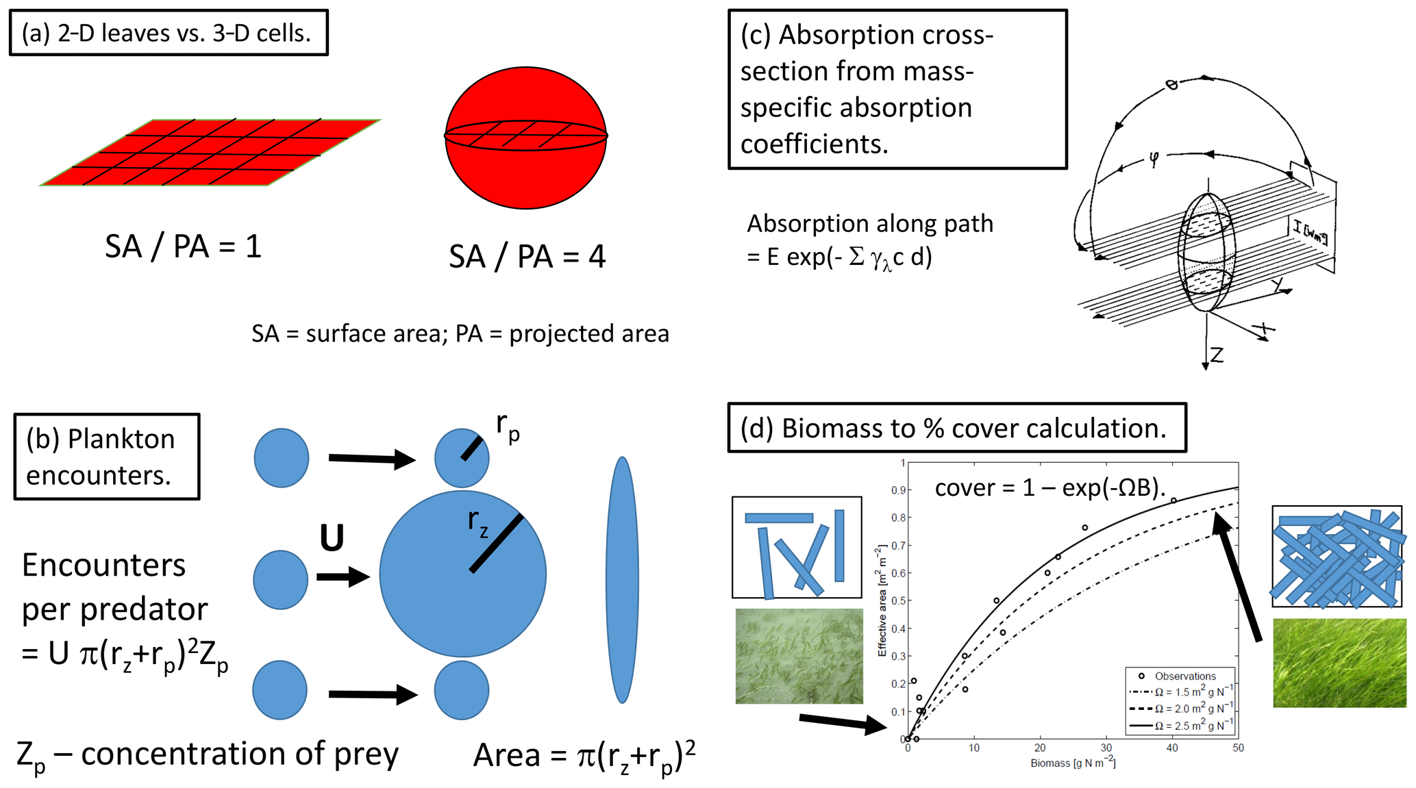
Figure 2Examples of geometric descriptions of ecological processes. (a) The relative difference in the 2-D experience to nutrient and light fields of leaves compared to the 3-D experience of cells, as typified by the ratio of surface area (coloured) to projected area (hashed area). (b) The encounter rate of prey per individual predator as a function of the radius of encounter (the sum of the predator and prey radii) and the relative motion and prey concentration following Jackson (1995). (c) The use of ray tracing and the mass-specific absorption coefficient to calculate an absorption cross-section for a randomly oriented spheroid following Kirk (1975). (d) Fraction of the bottom covered as seen from above as a result of increasing the number of randomly placed leaves (Baird et al., 2016a), based on the assumption that leaves are randomly placed; the cover reaches when the sum of the shaded areas induced by all individual leaves equals the ground area (i.e. a leaf area index of 1).
Perhaps the most important consequence of using geometric constraints in the BGC model is the representation of benthic flora as two-dimensional surfaces, while plankton are represented as three-dimensional suspended objects (Baird and Middleton, 2004). Thus, leafy benthic plants such as macroalgae take up nutrients and absorb light on a 2-D surface. In contrast, nutrient uptake to microalgae occurs through a 3-D field, while light uptake of the 3-D cell is limited by the 2-D projected area (Fig. 2a). These contrasting geometric properties, from which the model equations are derived, generate greater potential light absorption relative to nutrient uptake of benthic communities relative to the same potential light absorption relative to nutrient uptake in unicellular algae (Baird et al., 2004). In the most simple terms, this can be related to the surface-area-to-projected-area ratio of a leaf being 0.25 times that of a microalgae cell (Fig. 2a). Thus, the competition for nutrients, ultimately being driven by light absorption and its rate compared to nutrient uptake, is explicitly determined by the contrasting geometries of cells and leaves.
In addition to geometric constraints derived by others, a number of novel geometric descriptions have been introduced into the EMS BGC model, including
-
geometric derivation of the relationship between biomass, B, and fraction of the bottom covered, , where Ω is the nitrogen-specific leaf area (Sect. 6);
-
impact of self-shading on chlorophyll synthesis quantified by the incremental increase in absorption with the increase in pigment content (Sect. 5.1.3);
-
mass-specific absorption coefficients of photosynthetic pigments better utilised to determine phytoplankton absorption cross-sections (Duysens, 1956; Kirk, 1975; Morel and Bricaud, 1981) through the availability of a library of mass-specific absorption coefficients (Clementson and Wojtasiewicz, 2019) and their wavelength correction using the refractive index of the solvent used in the laboratory determinations (Fig. 5);
-
the space limitation of zooxanthellae within coral polyps using zooxanthellae projected areas in a two-layer gastrodermal cell anatomy (Sect. 6.3.1); and
-
preferential ammonium uptake, which is often calculated using different half-saturation coefficients of nitrate and ammonium uptake (Lee et al., 2002), determined by allowing ammonium uptake to proceed up to the diffusion limit. Should this diffusion limit not meet the required demand, nitrate uptake supplements the ammonium uptake. This representation has the benefit that no additional parameters are required to assign preference, with the same approach applied for both microalgae and benthic plants (Sect. 9.1).
To be clear, these geometric definitions have their own set of assumptions (e.g. a single cell size for a population) and simplifications (e.g. spherical shape). Nonetheless, the effort to apply geometric descriptions of physical limits across the BGC model appears to have been beneficial, as measured by the minimal amount of re-parameterisation that has been required to apply the model to contrasting environments. Of the above-mentioned new formulations, the most useful and easily applied is the bottom cover calculation (Fig. 2d). In fact, it is so simple, and such a clear improvement on empirical forms as demonstrated in Baird et al. (2016a), that it is likely to have been applied in other ecological/biogeochemical models, although we are unaware of any other implementation.
The geometrically constrained relationship between bottom cover and seagrass biomass, B, is and can be used to illustrate how geometric arguments can produce model equations with tightly constrained parameters. This geometric relationship contains only one parameter, Ω, that is the initial slope between cover and biomass. At low biomass, there is no overlapping of leaves, so the Ω is the area of leaves per unit of biomass (or nitrogen-specific leaf area) and has been determined by many authors in hundreds of seagrass studies. Comparison with data is shown in Appendix A of Baird et al. (2016a) and Fig. 2d. Thus, by using geometric arguments in developing the equation, the form contains only one parameter which has a physical meaning that is tightly constrained.
In addition to using geometric descriptions, there are a few other features unique to the EMS BGC model including
-
calculation of scalar irradiance from downwelling irradiance, vertical attenuation and a photon balance within a layer (Sect. 4.1.2);
-
an oxygen balance achieved through use of biological and chemical oxygen demand tracers (Sect. 10.3.2); and
-
the stoichiometric link of excess photons to reactive oxygen production in zooxanthellae.
1.1 Paper outline
This document provides a summary of the biogeochemical processes included in the model (Sect. 2), a summary of the transport model that integrates the advection–diffusion and sinking terms (Sect. 3), and full descriptions of the optical (Sect. 4) and ecological (Sect. 5–9) model equations. The description of both the optical and biogeochemical models is divided into the primary environmental zones: pelagic, epibenthic and sediment. Sect. 9 details parameterisations that are common across numerous ecological processes, such as temperature dependence, and Sect. 10 provides details of the numerical integration techniques. Further sections detail the model evaluation (Sect. 11) and test case generation (Sect. 12). The discussion (Sect. 13) details how past and present applications have influenced the development of the EMS BGC model and anticipates some future developments. Code availability is detailed at the end of the paper. Finally, the Supplement provides tables of processes (S1), state variables (S3) and parameter values (S4), with both mathematical and numerical code details (S2), and additional model evaluation (S5), from the Great Barrier Reef configuration.
The optical and biogeochemical models are linked by the dependence of scattering and absorption on the state of optically active biogeochemical quantities. The optical model undertakes calculations at distinct wavelengths of light (say 395, 405, 415, … 705 nm) representative of individual wavebands (say 400–410, 410–420 nm, etc.) of the vertically resolved downwelling and scalar irradiance that are used by the biogeochemical model to drive photosynthesis. The optical model includes the effect of Earth–Sun distance, Sun angle, atmospheric transmission, surface albedo and refraction on the downwelling surface irradiance. In the water column, the model attenuates light based on the spectrally resolved total absorption and scattering of microalgae, detritus, dissolved organic matter, inorganic particles and the water itself (Fig. 3). The light reaching the bottom is further attenuated by macroalgae, seagrass, corals and benthic microalgae.
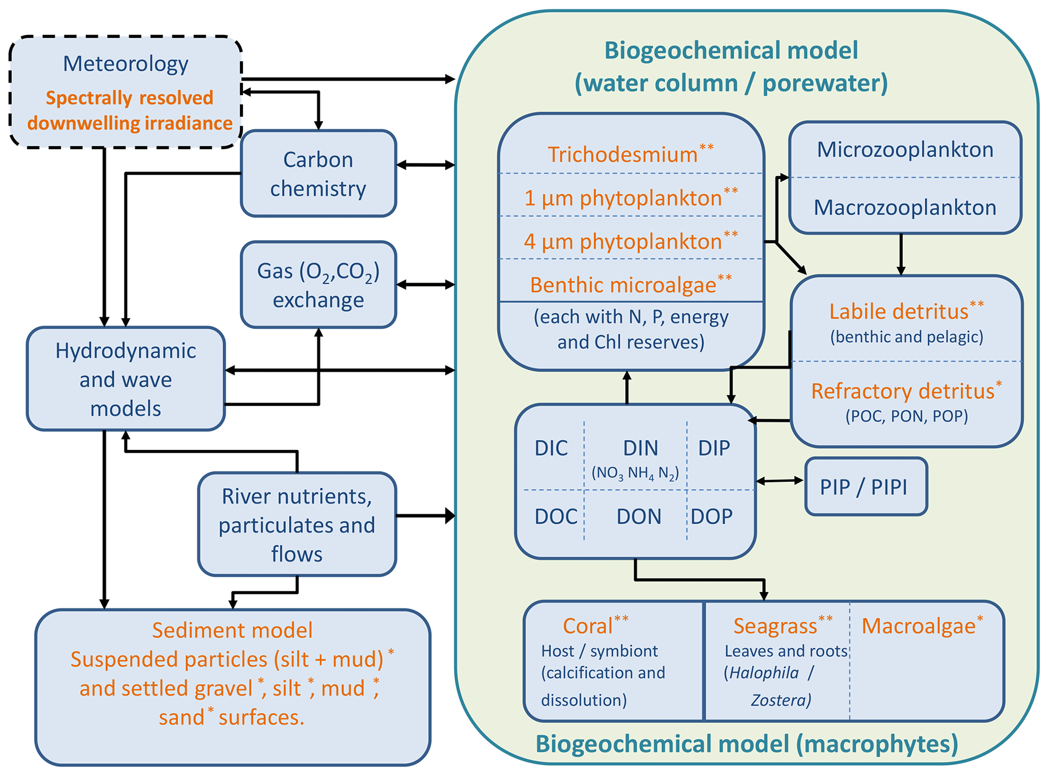
Figure 3Schematic of the CSIRO Environmental Modelling Suite illustrating the biogeochemical processes in the water column, epipelagic and sediment zones, as well as the carbon chemistry and gas exchange used in vB3p0 for the Great Barrier Reef application. Orange labels represent components that scatter or absorb light.
The biogeochemical model is organised into three zones: pelagic, epibenthic and sediment. Depending on the grid formulation, the pelagic zone may have one or many layers of similar or varying thickness. The epibenthic zone overlaps with the lowest pelagic layer and the top sediment layer and shares the same dissolved and suspended particulate material fields. The sediment is modelled in multiple layers with a thin layer of easily resuspendable material overlying thicker layers of more consolidated sediment. Each sediment layer contains both particles and porewater (Margvelashvili, 2009).
Dissolved and particulate biogeochemical tracers are advected and diffused throughout the model domain in an identical fashion to temperature and salinity. Additionally, biogeochemical particulate substances sink and are resuspended in the same way as sediment particles. Biogeochemical processes are organised into pelagic processes of phytoplankton and zooplankton growth and mortality, detritus remineralisation and fluxes of dissolved oxygen, nitrogen and phosphorus; epibenthic processes of growth and mortality of macroalgae, seagrass and corals, and sediment-based processes of plankton mortality, microphytobenthos growth, detrital remineralisation and fluxes of dissolved substances (Fig. 3).
The biogeochemical model considers four groups of microalgae (small and large phytoplankton representing the functionality of photosynthetic cyanobacteria and diatoms, respectively, microphytobenthos and Trichodesmium), four macrophytes types (seagrass types corresponding to Zostera, Halophila, deep Halophila and macroalgae) and coral polyps. For temperate system applications of the EMS, dinoflagellates, Nodularia and multiple macroalgal species have also been characterised (Wild-Allen et al., 2013; Hadley et al., 2015a).
Photosynthetic growth is determined by concentrations of dissolved nutrients (nitrogen and phosphate) and photosynthetically active radiation. Autotrophs take up dissolved ammonium, nitrate, phosphate and inorganic carbon. Microalgae incorporate carbon (C), nitrogen (N) and phosphorus (P) at the Redfield ratio (), while macrophytes do so at the Atkinson ratio (). Microalgae contain chlorophyll a and a suite of accessories pigments, and have variable carbon : pigment ratios determined using a photo-adaptation model.
Micro- and mesozooplankton graze on small and large phytoplankton, respectively, at rates determined by particle encounter rates and maximum ingestion rates. Additionally, large zooplankton consume small zooplankton. Of the grazed material that is not incorporated into zooplankton biomass, a fraction is released as dissolved and particulate carbon, nitrogen and phosphate, with the remainder forming detritus. Additional detritus accumulates by mortality. Detritus and dissolved organic substances are remineralised into inorganic carbon, nitrogen and phosphate with labile detritus transformed most rapidly (days), refractory detritus slower (months) and dissolved organic material transformed over the longest timescales (years). The production (by photosynthesis) and consumption (by respiration and remineralisation) of dissolved oxygen is also included in the model and, depending on prevailing concentrations, facilitates or inhibits the oxidation of ammonium to nitrate and its subsequent denitrification to dinitrogen gas which is then lost from the system.
Additional water column chemistry calculations are undertaken to solve for the equilibrium carbon chemistry ion concentrations necessary to undertake ocean acidification (OA) studies and to consider sea–air fluxes of oxygen and carbon dioxide. The adsorption and desorption of phosphorus onto inorganic particles as a function of the oxic state of the water are also considered.
In the sediment porewaters, similar remineralisation processes occur as in the water column (Fig. 4). Additionally, nitrogen is denitrified and lost as N2 gas, while phosphorus can become adsorbed onto inorganic particles and become permanently immobilised in sediments.
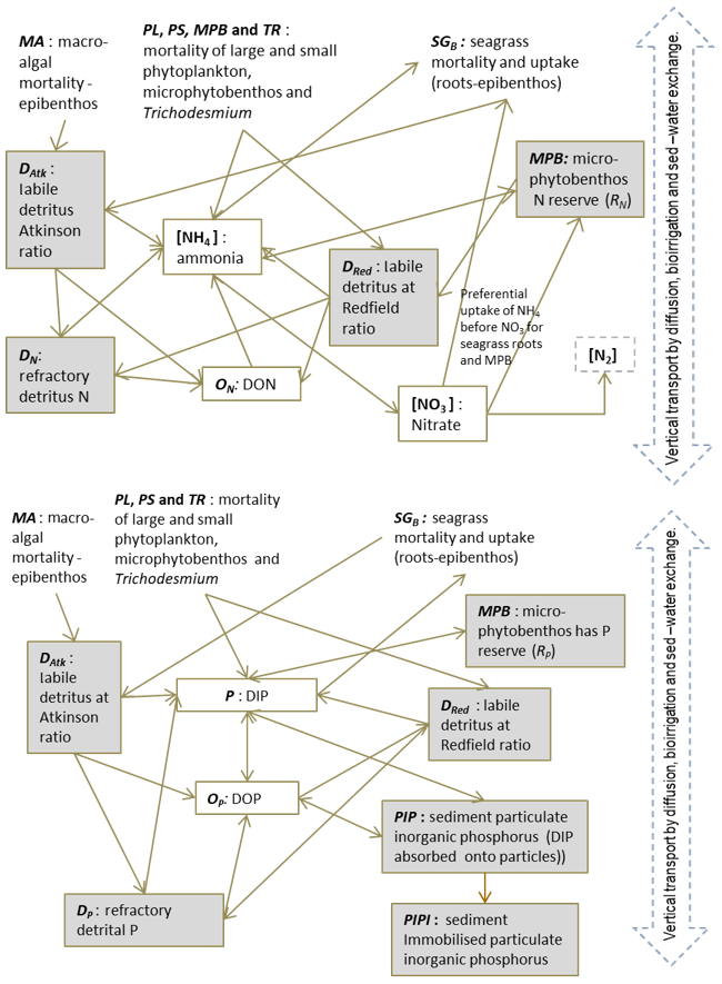
Figure 4Schematics of sediment nitrogen (top) and phosphorus (bottom) pools and fluxes. Processes represented include phytoplankton mortality, detrital decomposition, denitrification (nitrogen only), phosphorus adsorption (phosphorus only) and microphytobenthic growth. Grey boxes are particles.
2.1 Structure of the model description
The biogeochemical model presented in this paper is process based. That is, the rate of change of each ecological state variable is determined by a mathematical representation of each process that moves mass between one variable and another, conserving total mass. For dissolved inorganic phosphorus, the equation in the bottom water column layer (excluding advection, diffusion and particle sinking) could be written as
As the number of processes in the model has grown, the representation of all the terms affecting one variable has become unworkable. Thus, instead of presenting the full equation for each state variable, we present the full set of equations for each process.
2.1.1 Presentation of process equations
In Sects. 5–9, descriptions are sorted by processes, such as microalgae growth, coral growth and food web interactions. This organisation allows the model to be explained, with individual notation, in self-contained chunks. For each process, the complete set of model equations, parameter values and state variables is given in tables. Within each process, the equations are required to conserve mass of oxygen, carbon, nitrogen and phosphorus. Furthermore, each process description is independent of any other processes in the model. As the code itself allows the inclusion/exclusion of processes at runtime, the process-based structuring of the scientific description aligns with the architecture of the numerical code.
2.1.2 Model stoichiometry
The model contains state variables that quantify the mass of carbon, nitrogen, phosphorus and oxygen, as well as state variables that contain stoichiometrically constant combinations of carbon, nitrogen, phosphorus ( of for plankton and animals; for benthic plants). While the majority of the state variables and parameters are specified in units of nitrogen, the model could equally be specified by carbon or phosphorus. Furthermore, while the structural material of microalgae (including benthic microalgae and zooxanthellae) is at the Redfield ratio, changing reserves in microalgae of fixed carbon, nitrogen and phosphorus mean that the microalgae have a variable stoichiometry. The model has separate state variables for refractory detrital carbon, nitrogen and phosphorus, so the sum of all refractory detritus components has a variable stoichiometry. As explained later, we represent stoichiometric coefficients in the model equations as integers, a simple approximation (Table 41) to improve the readability of the mathematical equations.
The local rate of change of concentration, C, of each dissolved and particulate constituent contains sink/source terms, SC, which are described in length in the process descriptions of this document, and the advection, diffusion and sinking terms:
where the symbol , v is the velocity field, K is the eddy diffusion coefficient which varies in space and time, and wsink is the local sinking rate (positive downwards) with the z coordinate positive upwards. The calculation of v and K is described in the hydrodynamic model (Herzfeld, 2006; Gillibrand and Herzfeld, 2016). The advection–diffusion terms of Eq. (1), based on the continuum hypothesis for a fluid (Vichi et al., 2007), are solved by either an in-line advection scheme with the baroclinic time step of the hydrodynamic model or an offline transport scheme using a potentially much longer time step (Gillibrand and Herzfeld, 2016). Options for advection and transport schemes in EMS include mass conservative Lagrangian and flux-form approaches described in Herzfeld (2006) and Gillibrand and Herzfeld (2016).
The microalgae are particulates that contain internal concentrations of dissolved nutrients (C, N, P) and pigments that are specified on a per cell basis. To conserve mass, the local rate of change of the concentration of microalgae, B, multiplied by the content (or reserve) of the cell, R, is given by
For more information, see Sect. 5.1.6 and Sect. 3.1 of Baird et al. (2004) which describe the coupling of the plankton component of the biogeochemical model to the Princeton Ocean Model.
The optical model calculates the spectrally resolved light field in each vertical column and uses it to drive the photosynthesis of phytoplankton and benthic plants in the biogeochemical model. Following the terminology of aquatic optics (Mobley, 1994), we divide the description of the model into calculations of inherent optical properties (IOPs) followed by apparent optical properties (AOPs). IOPs are properties of the medium (e.g. scattering and absorption) and do not depend on the ambient light field. The optical model uses the value of the optically active state variables, and their mass-specific absorption and scattering properties, to calculate the total absorption and scattering. AOPs are those properties that depend both on the medium (the IOPs) and on the surface light field. AOPs include downwelling and scalar irradiance. Thus, the optical model uses the vertical distribution of IOPs, and the surface light field, to determine the vertical distribution of the AOPs.
4.1 Water column optical model
4.1.1 Inherent optical properties (IOPs)
Phytoplankton absorption. The model contains four phytoplankton types (small and large phytoplankton, benthic microalgae and Trichodesmium), each with a unique ratio of internal concentration of accessory photosynthetic pigments to chlorophyll a. To calculate the absorption due to each pigment, we use a database of spectrally resolved mass-specific absorption coefficients (Clementson and Wojtasiewicz, 2019). As it can be assumed that accessory pigments stay in a constant ratio to chlorophyll a, the model needs only a state variable for chlorophyll a for each phytoplankton type. The model then calculates the chlorophyll a specific absorption coefficient due to all pigments by using a state variable quantifying the chlorophyll concentration of the population, the number of cells in the population and the ratio of concentration of the accessory pigment to chlorophyll a, and the mass-specific absorption coefficient of each of the accessory pigments. Thus, the chlorophyll a specific absorption coefficient due to all photosynthetic pigments for small phytoplankton at wavelength λ, γsmall,λ, is given by
where Chl a is the pigment chlorophyll a, Zea is zeaxanthin, Echi is echinenone, β-car is β carotene, PE is phycoerythrin, and PC is phycocyanin, and the ratios of chlorophyll a to accessory pigment concentration are determined from Wojtasiewicz and Stoń-Egiert (2016). Note that the coefficient in Eq. (3) for Chl a is 1.0 because the ratio of chlorophyll a to chlorophyll a is 1. The resulting chlorophyll a specific absorption coefficient for picoplankton is shown in Fig. 5.
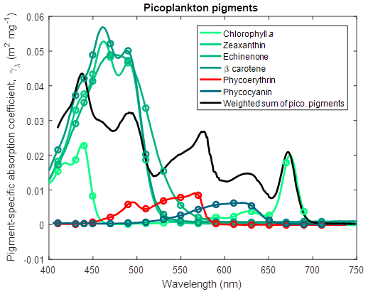
Figure 5Pigment-specific absorption coefficients for the dominant pigments found in small phytoplankton determined using laboratory standards in solvent in a 1 cm vial. Green and red lines are photosynthetic pigments constructed from 563 measured wavelengths. Circles represent the wavelengths at which the optical properties are calculated in the simulations. The black line represents the weighted sum of the photosynthetic pigments (Eq. 3), with the weighting calculated from the ratio of each pigment concentration to chlorophyll a. The spectra are wavelength shifted from their raw measurement by the ratio of the refractive index of the solvent to the refractive index of water (1.352 for acetone used with chlorophyll a and β carotene; 1.361 for ethanol used with zeaxanthin and echinenone; 1.330 for water used with phycoerythrin and phycocyanin).
Similarly, for large phytoplankton and microphytobenthos (Wright et al., 1996),
where Fuco is fucoxanthin (Fig. 6) and for Trichodesmium (Carpenter et al., 1993),
where Myxo is myxoxanthophyll (Fig. 7).
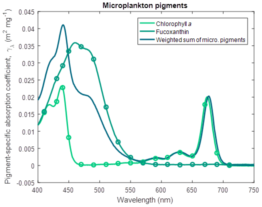
Figure 6Pigment-specific absorption coefficients for the dominant pigments found in large phytoplankton and microphytobenthos determined using laboratory standards in solvent in a 1 cm vial. The aqua line represents the weighted sum of the photosynthetic pigments (Eq. 4), with the weighting calculated from the ratio of each pigment concentration to chlorophyll a. See Fig. 5 for more details. Fucoxanthin was dissolved in ethanol.
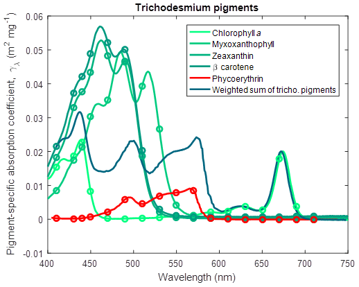
Figure 7Pigment-specific absorption coefficients for the dominant pigments found in Trichodesmium determined using laboratory standards in solvent in a 1 cm vial. The aqua line represents the weighted sum of the photosynthetic pigments (Eq. 5), with the weighting calculated from the ratio of each pigment concentration to chlorophyll a. See Fig. 5 for more details. Myxoxanthophyll was dissolved in acetone.
The absorption cross-section at wavelength λ (αλ) of a spherical cell of radius (r), chlorophyll a specific absorption coefficient (γλ) and homogeneous intracellular chlorophyll a concentration (ci) can be calculated using geometric optics (i.e. ray tracing without considering internal scattering) and is given by (Duysens, 1956; Kirk, 1975)
where πr2 is the projected area of a sphere, and the bracketed term is 0 for no absorption (γcir=0) and approaches 1 as the cell becomes fully opaque (γcir→∞). Note that the bracketed term in Eq. (6) is mathematically equivalent to the dimensionless efficiency factor for absorption, Qa (used in Morel and Bricaud, 1981, Finkel, 2001 and Bohren and Huffman, 1983), of homogeneous spherical cells with an index of refraction close to that of the surrounding water. Note that the intracellular chlorophyll concentration, ci, changes as a result of chlorophyll synthesis (described later in Eq. 34).
The use of an absorption cross-section of an individual cell has two significant advantages. Firstly, the same model parameters used here to calculate absorption in the water column are used to determine photosynthesis by individual cells, including the effect of packaging of pigments within cells. Secondly, the dynamic chlorophyll concentration determined later can be explicitly included in the calculation of phytoplankton absorption. Thus, the absorption of a population of n cell m−3 is given by nα m−1, while an individual cell absorbs αEo light, where Eo is the scalar irradiance.
Coloured dissolved organic matter (CDOM) absorption. Two equations for CDOM absorption are presently being trialled. The two schemes are as follows: Scheme 1. The absorption of CDOM, aCDOM,λ, is determined from a relationship with salinity in the region (Schroeder et al., 2012):
where S is the salinity. In order to avoid unrealistic extrapolation, the salinity used in this relationship is the minimum of the model salinity and 36. In some cases, coastal salinities exceed 36 due to evaporation. The absorption due to CDOM at other wavelengths is calculated using a CDOM spectral slope for the region (Blondeau-Patissier et al., 2009):
where SCDOM is an approximate spectral slope for CDOM, with observations ranging from 0.01 to 0.02 nm−1 for significant concentrations of CDOM. Lower magnitudes of the spectral slope generally occur at lower concentrations of CDOM (Blondeau-Patissier et al., 2009).
Scheme 2. The absorption of CDOM, aCDOM,λ, is directly related to the concentration of dissolved organic carbon, DC:
where is the dissolved organic carbon-specific CDOM absorption coefficient at 443 nm.
Both schemes have drawbacks. Scheme 2, using the concentration of dissolved organic carbon, is closer to reality but is likely to be sensitive to poorly known parameters such as remineralisation rates and initial detritial concentrations. Scheme 1, a function of salinity, will be more stable but perhaps less accurate, especially in estuaries where hypersaline waters may have large estuarine loads of coloured dissolved organic matter.
Absorption due to non-algal particulate material. The waters of the Great Barrier Reef contain suspended sediments originating from various marine sources, such as the white calcium carbonate fragments generated by coral erosion and sediments derived from terrestrial sources such as granite (Soja-Woźniak et al., 2019). The model uses spectrally resolved mass-specific absorption coefficients (and also total scattering measurements) from a database of laboratory measurements conducted on either pure mineral suspensions, or mineral mixtures, at two ranges of size distributions (Fig. 8; Stramski et al., 2007). In this model version, we use the calcium carbonate sample CAL1 for CaCO3-based particles.
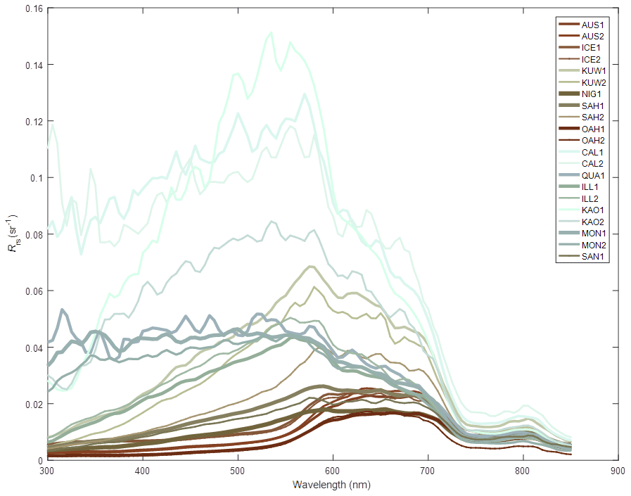
Figure 8The remote-sensing reflectance of the 21 mineral mixtures suspended in water as measured by Stramski et al. (2007). Laboratory measurements of absorption and scattering properties are used to calculated remote-sensing reflectance (Baird et al., 2016b). Line colouring corresponds to that produced by the mineral suspended in clear water as calculated using the MODIS true colour algorithm (Gumley et al., 2010). CAL1, with a median particle diameter of 2 µm, is used for Mud.
For the terrestrially sourced particles, we used observations from Gladstone Harbour in the central Great Barrier Reef (GBR) (Fig. 9). These IOPs gave a realistic surface colour for the Queensland river sediment plumes (Baird et al., 2016b). In the model, optically active non-algal particulates (NAPs) include the inorganic particulates (such as sand and mud; see Sect. 7.1) and detritus. We assumed the optical properties of the detritus were the same as the optical properties in Gladstone Harbour, although open-ocean studies have used a detritial absorption that is more like CDOM (Dutkiewicz et al., 2015).
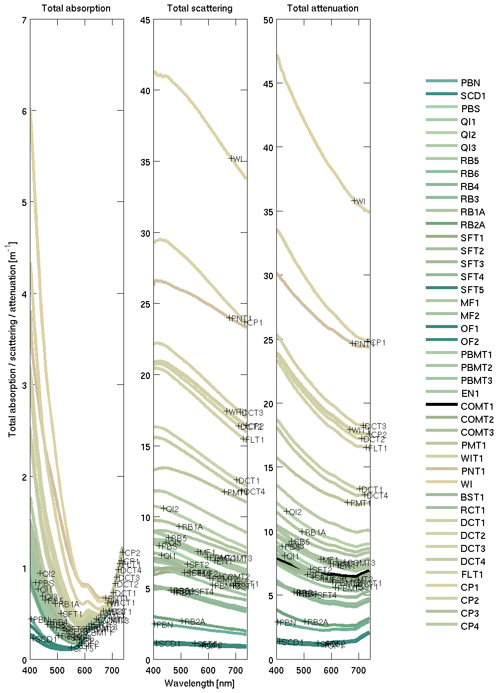
Figure 9Inherent optical properties (total absorption and total scattering) at sample sites in Gladstone Harbour on 13–19 September 2013 (Babcock et al., 2015). The line colour is rendered like that in Fig. 8. The site labelling is ordered in time, from the first sample collected during neap tides at the top to the last sample collected at spring tides on the bottom. The IOPs used for the Mud end-member are from the WIT site (see legend) at the centre of the harbour, was dominated by inorganic particles. The measured concentration of NAP at the site was 33.042 mg L−1 and is used to calculate mass-specific IOPs.
The absorption due to calcite-based NAP is given by
where c1 is the spectrally resolved mass-specific absorption coefficient determined from laboratory experiments (Fig. 8). The absorption due to non-calcite NAPs, NAP, combined with detritus, is given by
where c2 is the spectrally resolved mass-specific absorption coefficient determined from field measurements (Fig. 9), NAP is quantified in kg m−3, DAtk and DRed are quantified in mg N m−3, and DC is quantified in mg C m−3.
Total absorption. The total absorption, aT,λ, is given by
where aw,λ is clear-water absorption (Fig. 10) and N is the number of phytoplankton classes (see Table 3).
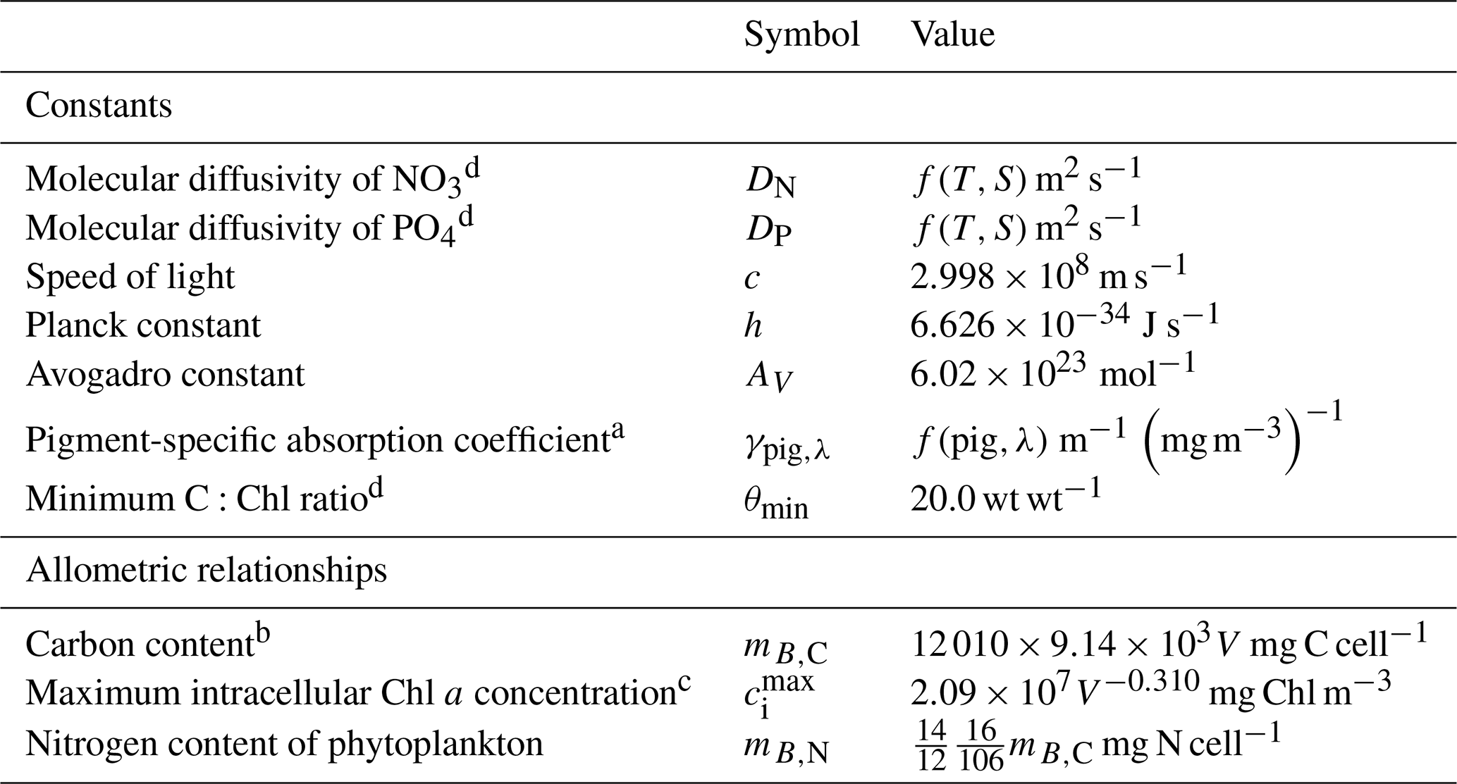
Table 1Constants and parameter values used in the optical model.
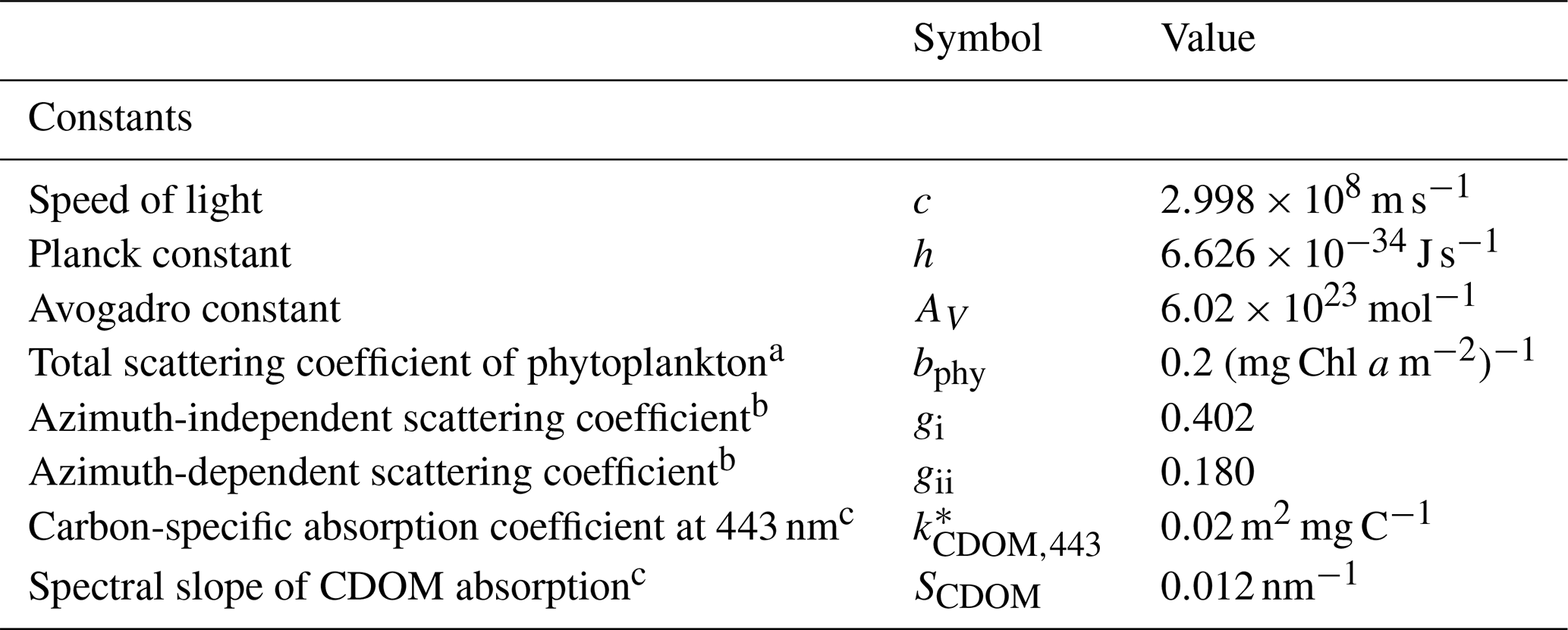
a Kirk (1994). b Kirk (1991) using an average cosine of scattering of 0.924 (Mobley, 1994). c Blondeau-Patissier et al. (2009); see also Cherukuru et al. (2019).
Table 2State and derived variables in the water column optical model.
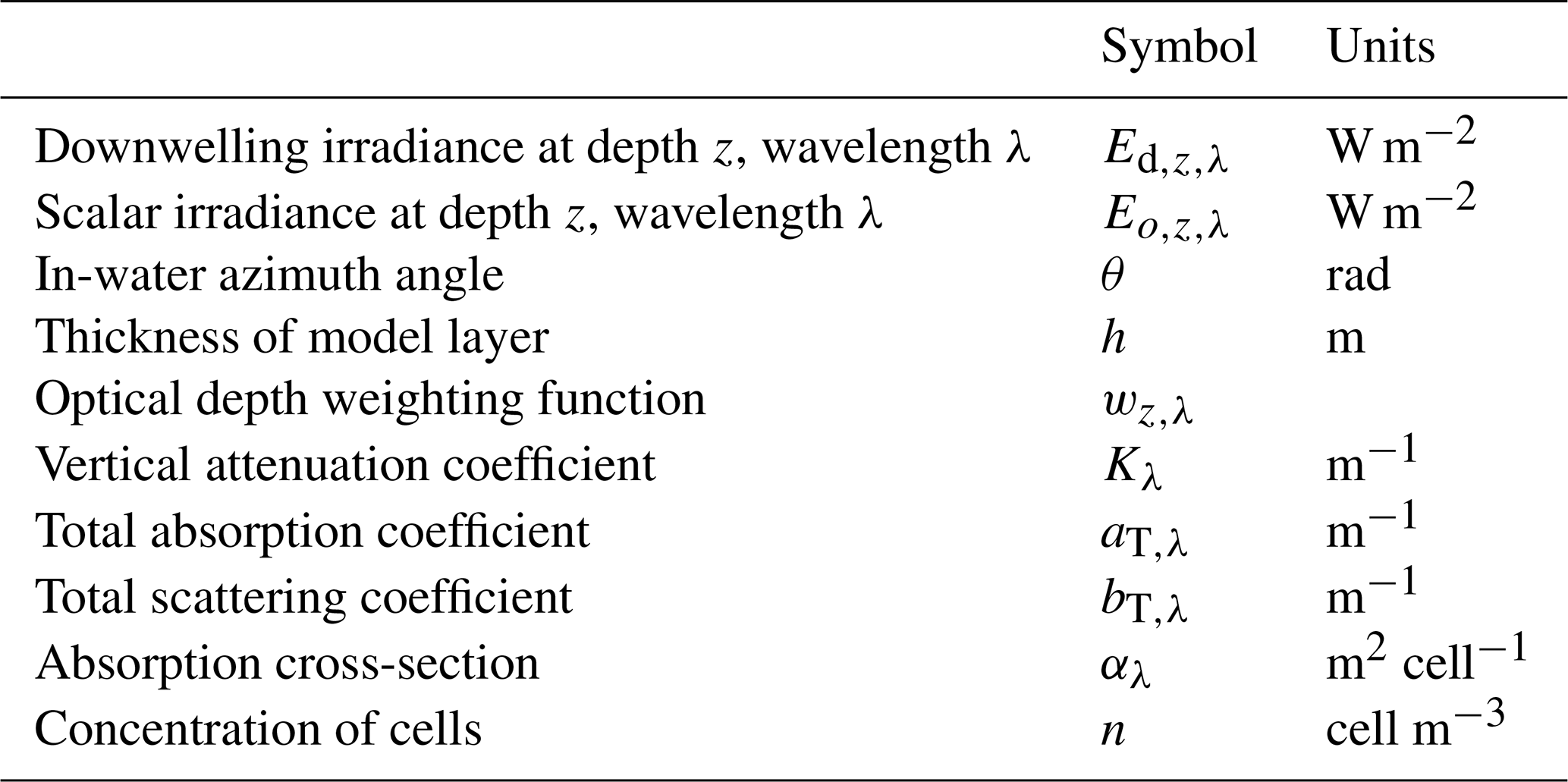
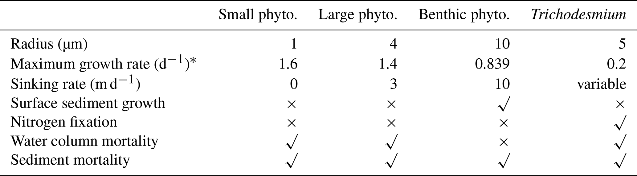
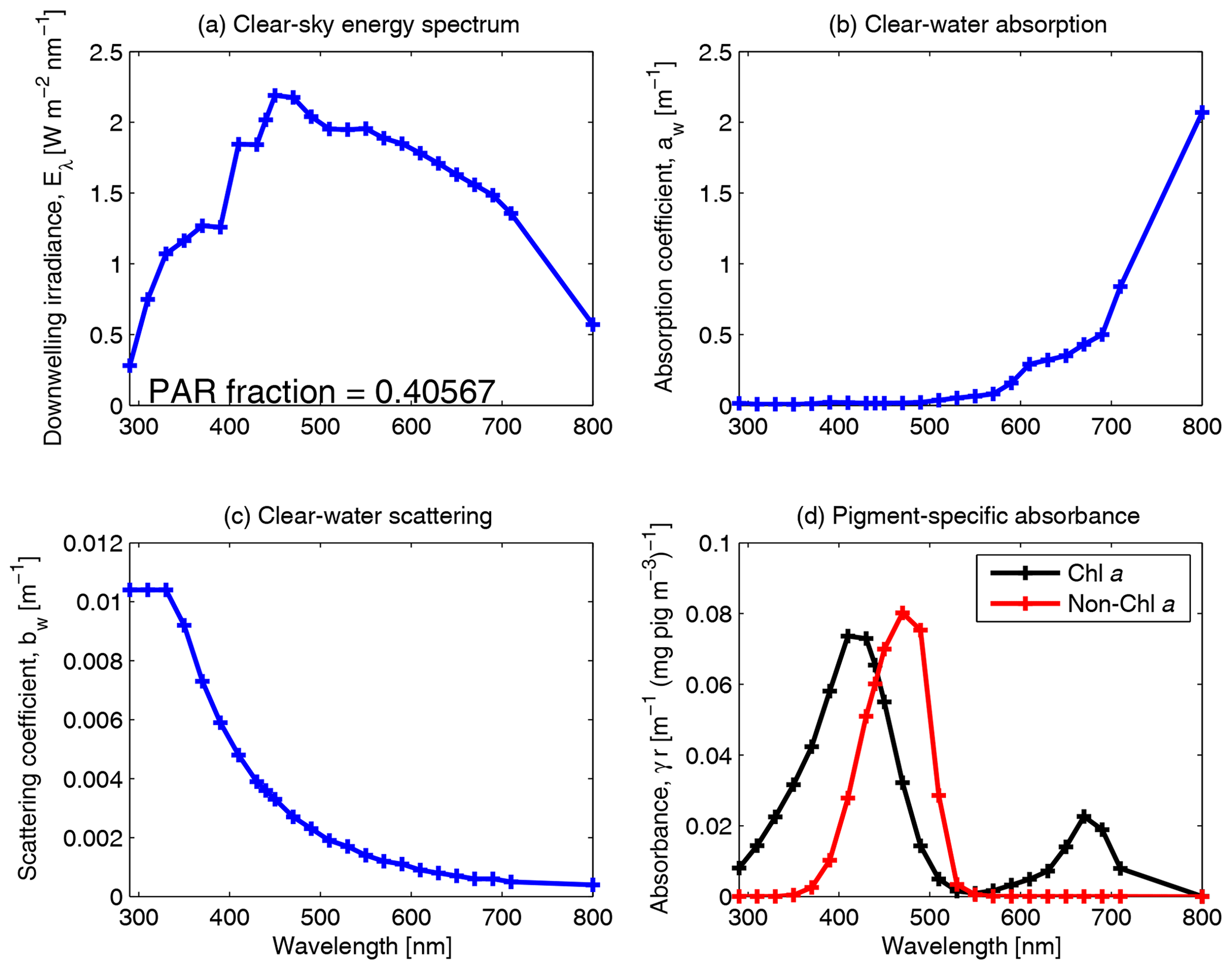
Figure 10Spectrally resolved energy distribution of sunlight, clear-water absorption and clear-water scattering (Smith and Baker, 1981). The fraction of solar radiation between 400 and 700 nm for clear-sky irradiance at the particular spectral resolution is given in panel (a). The centre of each waveband used in the model simulations is identified by a cross on each curve. Panel (d) shows the pigment-specific absorption of Chl a and generic photosynthetic carotenoids (Ficek et al., 2004) that were used in earlier versions of this model (Baird et al., 2016b) before the mass-specific absorption coefficients of multiple accessory pigments were implemented (Figs. 5, 6 and 7).
Scattering. The total scattering coefficient is given by
where NAP is the concentration of non-algal particulates, bw,λ is the scattering coefficient due to clear water (Fig. 10), c1 and c2 are the spectrally resolved mass-specific coefficients (Figs. 8 and 9) and phytoplankton scattering is the product of the chlorophyll-specific phytoplankton scattering coefficient, bphy,λ and the water column chlorophyll concentration of all classes, (where ci is the chlorophyll concentration in the cell, and V is the cell volume). The value for bphy,λ is set to 0.2 (mg Chl a m−2)−1 for all wavelengths, a typical value for marine phytoplankton (Kirk, 1994). For more details, see Baird et al. (2007b).
4.1.2 Apparent optical properties (AOPs)
The optical model is forced with the downwelling short-wave radiation just above the sea surface, based on remotely sensed cloud fraction observations and calculations of top-of-the-atmosphere clear-sky irradiance and solar angle. The calculation of downwelling radiation and surface albedo (a function of solar elevation and cloud cover) is detailed in Sect. 9.1.1 of the hydrodynamic scientific description (https://research.csiro.au/cem/software/ems/ems-documentation/, last access: 22 September 2020).
The downwelling irradiance just above the water interface is split into wavebands using the weighting for clear-sky irradiance (Fig. 10). Snell's law is used to calculate the azimuth angle of the mean light path through the water, θsw, as calculated from the atmospheric azimuth angle, θair, and the refraction of light at the air–water interface (Kirk, 1994):
Calculation of in-water light field. Given the IOPs determined above, the exact solution for AOPs would require a radiative transfer model (Mobley, 1994) which is too computationally expensive for a complex ecosystem model such as developed here. Instead, the in-water light field is solved for using empirical approximations of the relationship between IOPs and AOPs (Kirk, 1991; Mobley, 1994).
The vertical attenuation coefficient at wavelength λ when considering absorption and scattering, Kλ, is given by
The term outside the square root quantifies the effect of absorption, where aT,λ is the total absorption. The term within the square root of Eq. (15) represents scattering as an extended pathlength through the water column, where gi and gii are empirical constants and take values of 0.402 and 0.180, respectively. The values of gi and gii depend on the average cosine of scattering. For filtered water with scattering only due to water molecules, the values of gi and gii are quite different to natural waters. But for waters ranging from coastal to open ocean, the average cosine of scattering varies by only a small amount (0.86–0.95; Kirk, 1991), and thus uncertainties in gi and gii do not strongly affect Kλ.
The downwelling irradiance at wavelength λ at the bottom of a layer h thick, , is given by
where is the downwelling irradiance at wavelength λ at the top of the layer and Kλ is the vertical attenuation coefficient at wavelength λ, a result of both absorption and scattering processes.
Assuming a constant attenuation rate within the layer, the average downwelling irradiance at wavelength λ, Ed,λ, is given by
We can now calculate the scalar irradiance, Eo, for the calculation of phytoplankton absorption, from downwelling irradiance, Ed. The light absorbed within a layer must balance the difference in downwelling irradiance from the top and bottom of the layer (since scattering in this model only increases the pathlength of light); thus,
Cancelling h, the scalar irradiance as a function of downwelling irradiance is given by
This correction conserves photons within the layer, although it is only as good as the original approximation of the impact of scattering and azimuth angle on vertical attenuation (Eq. 15).
Vertical attenuation of heat. The vertical attenuation of heat is given by
and the local heating by
where T is temperature, ρ is the density of water, and cp is the specific heat of water.
4.2 Epibenthic optical model
The spectrally resolved light field at the base of the water column is attenuated, from top to bottom, by macroalgae and seagrass (Zostera, then shallow and then deep forms of Halophila), followed by the zooxanthellae in corals. The downwelling irradiance at wavelength λ after passing through each macroalgae and seagrass species is given by Ebelow,λ:
where Eabove,λ for macroalgae is , the downwelling irradiance of the bottom water column layer, Aλ is the leaf-specific absorptance, Ω is the nitrogen-specific leaf area, and X is the leaf nitrogen biomass.
The light absorbed by corals is assumed to be entirely due to zooxanthellae and is given by
where is the areal density of zooxanthellae cells and αλ is the absorption cross-section of a cell a result of the absorption of multiple pigment types.
4.3 Sediment optical model
The optical model in the sediment only concerns the benthic microalgae growing in the porewaters of the top sediment layer. The calculation of light absorption by benthic microalgae assumes they are the only attenuating component in a layer that lies on top layer of sediment, with a perfectly absorbing layer below and no scattering by any other components in the layer. Thus, no light penetrates through to the second sediment layer where benthic microalgae also reside. Thus, the downwelling irradiance at wavelength λ at the bottom of a layer, , is given by
where is the downwelling irradiance at wavelength λ at the top of the layer and αλ is the absorption cross-section of the cell at wavelength λ, and n is the concentration of cells in the layer. The layer thickness used here, h, is the thickness of the top sediment layer, so as to convert the concentration of cells in that layer, n, into the areal concentration of cells in the biofilm, n h.
Given no scattering in the cell, and that the vertical attenuation coefficient is independent of azimuth angle, the scalar irradiance that the benthic microalgae is exposed to in the surface biofilm is given by
The photons captured by each cell, and the microalgae process, follow the same equations as for the water column (Sect. 5.1.3).
5.1 Microalgae
The model contains four functional groups of suspended microalgae: small and large phytoplankton, microphytobenthos and Trichodesmium. The growth from internal reserves for each of the functional groups is identical and explained below. The differences in the ecological interactions of the four functional groups are summarised in Table 3. Trichodesmium, a nitrogen fixer, contains additional processes (Sect. 5.2).
5.1.1 Microalgal growth
The growth of microalgae has been modelled in many ways, from simple exponential growth and logistic growth curves, to single- and multiple-nutrient-based curves, through to equations that contain a state variable for the physiological state of the cell (variously described as stores, quotas, reserves, etc.) and to consider the complex processing of photons in the microalgae photosystem. It is now common for complex biogeochemical models to contain state variables for the physiological state of each of the potentially limiting nutrients (Baretta-Bekker et al., 1997; Vichi et al., 2007) and include adaptation to photosystems (Geider et al., 1998). In the context of many different microalgae models, the model that is described here has taken another path again. As articulated above, we chose to base nutrient uptake and light absorption on using geometric constraints. This meant that any growth model needed to be formulated around the maximum rate of supply of each of the limiting nutrients (and light) (see Fig. 2 of Baird et al., 2006).
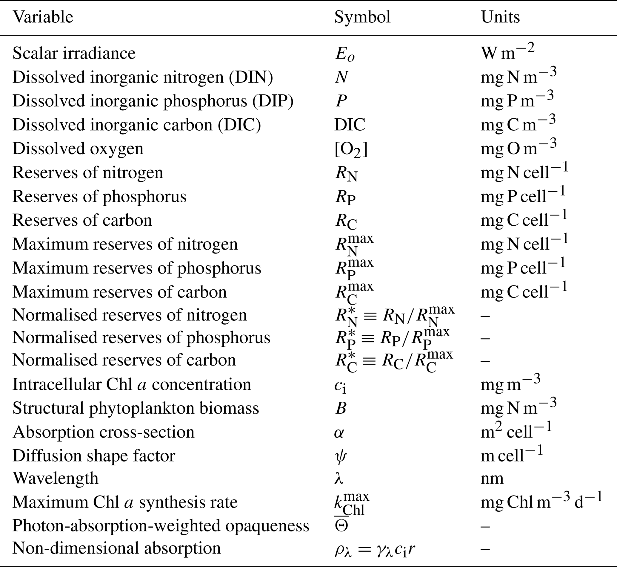
In the microalgae model (most fully described in Baird et al., 2001), the uptake of nutrients and light absorption increases the reserves of nutrients and light, as quantified by a reserve, R, which has units of mass per cell. In the equations, we often use a normalised reserve, R*, which is a quantity between 0 and 1 (Table 4). The reserves are in turn consumed to generate structural material. Thus, the total content of nitrogen in the microalgae is equal to the sum of the structural material and the reserves.
Table 4State and derived variables for the microalgae growth model. DIN is given by the sum of nitrate and ammonium concentrations, [NO3]+[NH4].
The model considers the diffusion-limited supply of dissolved inorganic nutrients (N and P) and the absorption of light, delivering N, P and fixed C to the internal reserves of the cell (Fig. 11). Nitrogen and phosphorus are taken directly into the reserves, but carbon is first fixed through photosynthesis (Kirk, 1994):
The internal reserves of C, N and P are consumed to form structural material at the Redfield ratio (Redfield et al., 1963):
where we have represented nitrogen as ammonium (NH4) in Eq. (27). When the nitrogen source to the cell is nitrate, NO3, it is assumed to lose its oxygen at the cell wall (Sect. 9.1). The growth rate of microalgae is given by the maximum growth rate, μmax, multiplied by the normalised reserves, R*, of each of C, N and P:
The mass of the reserves (and therefore the total a ratio) of the cell depends on the interaction of the supply and consumption rates (Fig. 11). When consumption exceeds supply, and the supply rates are non-Redfield, the normalised internal reserves of the non-limiting nutrients approach 1, while the limiting nutrient becomes depleted. Thus, the model behaves like a “law of the minimum” growth model, except during fast changes in nutrient supply rates.
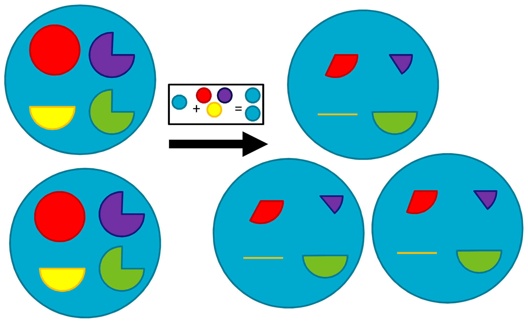
Figure 11Schematic of the process of microalgae growth from internal reserves. Blue circle: structural material; red pie: nitrogen reserves; purple pie: phosphorus reserves; yellow pie: carbon reserves; green pie: pigment content. Here, a circular pie has a value of 1, representing the normalised reserve (a value between 0 and 1). The box shows that generating structural material for an additional cell requires the equivalent of 100 % internal reserves of carbon, nitrogen and phosphorus of one cell. This figure shows the discrete growth of two cells to three, requiring both the generation of new structural material from reserves and the reserves being diluted as a result of the number of cells in which they are divided increasing from two to three. Thus, the internal reserves for nitrogen after the population increases from two to three is given by two from the initial two cells, minus one for building structural material of the new cell, shared across the three offspring, to give one-third. The same logic applies to carbon and phosphorus reserves, with phosphorus reserves being reduced to one-sixth and carbon reserves being exhausted. In contrast, pigment is not required for structural material so the only reduction is through dilution; the three-fourths content of two cells is shared among three cells to equal one-half in the three cells. This schematic shows one limitation of a population-style model whereby reserves are “shared” across the population (as opposed to individual-based modelling; Beckmann and Hense, 2004). A proof of the conservation of mass for this scheme, including under mixing of populations of suspended microalgae, is given in Baird et al. (2004). The model equations also include terms affecting internal reserves through nutrient uptake, light absorption, respiration and mortality that are not shown in this simple schematic.
The molar ratio of a cell, the addition of structural material and reserves, is given by
5.1.2 Nutrient uptake
The diffusion-limited nutrient uptake to a single phytoplankton cell, J, is given by
where ψ is the diffusion shape factor (=4πr for a sphere), D is the molecular diffusivity of the nutrient, Cb is the average extracellular nutrient concentration, and Cw is the concentration at the wall of the cell. The diffusion shape factor is determined by equating the divergence of the gradient of the concentration field in the vicinity of the cell to zero (∇2C=0). A semi-empirical correction to Eq. (30), to account for fluid motion around the cell, and the calculation of non-spherical diffusion shape factors, has been applied in earlier work (Baird and Emsley, 1999). For the purposes of biogeochemical modelling, these uncertain corrections for small-scale turbulence and non-spherical shapes are not quantitatively important and have not been pursued here.
Numerous studies have considered diffusion-limited transport to the cell surface at low nutrient concentrations saturating to a physiologically limited nutrient uptake at higher concentrations (Hill and Whittingham, 1955; Pasciak and Gavis, 1975; Mann and Lazier, 2006). The physiological limitation is typically considered using a Michaelis–Menten-type equation. Here, we simply consider the diffusion-limited uptake to be saturated by the filling up of reserves, . Thus, nutrient uptake is given by
where R* is the normalised reserve of the nutrient being considered. As shown later when considering preferential ammonium uptake, under extreme limitation relative to other nutrients, R* approaches 0, and uptake approaches the diffusion limitation.
5.1.3 Light capture and chlorophyll synthesis
Light absorption by microalgae cells has already been considered above (Eq. 6). The same absorption cross-section, α, is used to calculate the capture of photons per cell:
where accounts for the reduced capture of photons as the reserves becomes saturated, and converts from energy to photons. The absorption cross-section is a function of intracellular pigment concentration, which is a dynamic variable determined below. While a drop-off of photosynthesis occurs as the carbon reserves become replete, this formulation does not consider photo-inhibition due to photo-oxidative stress, although it has been considered elsewhere for zooxanthellae (Baird et al., 2018).
The rate of synthesis of pigment is based on the incremental benefit of adding pigment to the rate of photosynthesis. This calculation includes both the reduced benefit when carbon reserves are replete, , and the reduced benefit due to self-shading, χ. The factor χ is calculated for the derivative of the absorption cross-section per unit projected area (see Eq. 6), α∕PA, with non-dimensional group ρ=γcir. For a sphere of radius r (Baird et al., 2013),
where χ represents the area-specific incremental rate of change of absorption with ρ. The rate of chlorophyll synthesis is given by
where is the maximum rate of synthesis, θmin is the minimum C:Chl ratio, and the line in signifies the mean over the photosynthetically available radiation. At θmin, pigment synthesis is zero. Both self-shading and the rate of photosynthesis itself are based on photon absorption rather than energy absorption (Table 5), as experimentally shown in Nielsen and Sakshaug (1993).
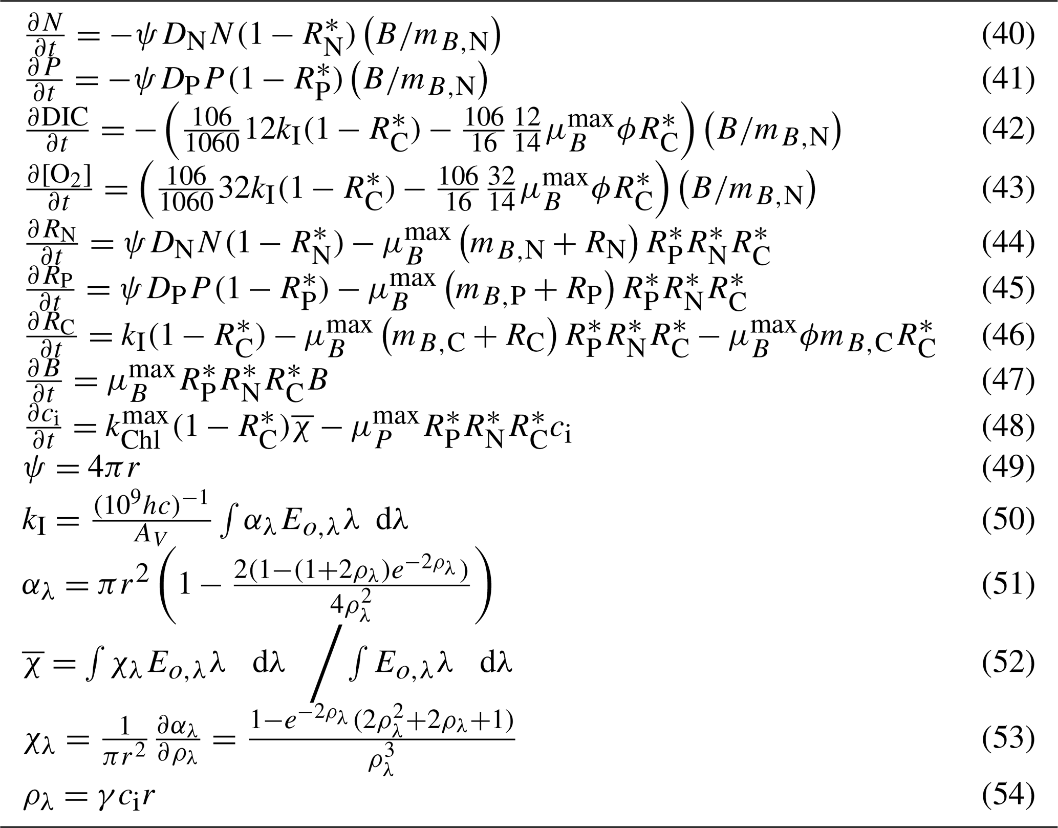
Table 5Microalgae growth model equations. The term is the concentration of cells. The equation for organic matter formation gives the stoichiometric constants: 12 g C mol C−1; 32 g O mol O2−1. The equations are for scalar irradiance specified as an energy flux.
For each phytoplankton type, the model considers multiple pigments with distinct absorption spectra. The model needs to represent all photo-absorbing pigments as the C:Chl model calculates the pigment concentration based on that required to maximise photosynthesis. If only Chl a was represented, the model would predict a Chl a concentration that was accounting for the absorption of Chl a and the auxiliary pigments, thus overpredicting the Chl a concentration when compared to observations.
5.1.4 Carbon fixation/respiration
When photons are captured, there is an increase in reserves of carbon, (Eq. 46), and an accompanying uptake of dissolved inorganic carbon, (Eq. 42), and release of oxygen, (Eq. 43), per cell to the water column (Table 5). Additionally, there is a basal respiration, representing a constant cost of cell maintenance. The loss of internal reserves, , results in a gain of water column dissolved inorganic carbon per cell, , as well as an uptake of dissolved oxygen per cell, (Table 5). The loss in water column dissolved oxygen per cell represents an instantaneous respiration of the fixed carbon reserves. Basal respiration decreases internal reserves, and therefore growth rate, but does not directly lead to cell mortality at zero carbon reserves. Implicit in this scheme is that the basal cost is higher when the cell has more carbon reserves, .
A linear mortality term, resulting in the loss of structural material and carbon reserves, is considered later.
5.1.5 Application of single cell rates to a population
As mentioned above, the nutrient uptake and light absorption rates are calculated on a per cell basis. This has allowed geometric considerations to be explicitly used and contrasts with most biogeochemical models that formulate planktonic rates based on population interactions. However, the state variables for microalgae (and zooplankton) are for the population. Therefore, rates per cell need to be multiplied by the number of cells to obtain population rates. In the case of microalgae, the number of cells n is given by . This assumes all cells in the population are identical and that the state variable for the population, B, is quantifying only the nitrogen (or oxygen, carbon and phosphorus) associated with the structural material. It should also be noted that all cells in a population have the same state of their reserves.
5.1.6 Conservation of mass of microalgae model
The conservation of mass of cells containing structural material and reserves during transport, growth and mortality is established in Baird et al. (2004). Briefly, for microalgal growth, total concentration of nitrogen in microalgae cells is given by . For conservation of mass, the time derivatives must equate to zero:
using the product rule to differentiate the second term on the left-hand side:
where
thus demonstrating conservation of mass when , as used here.
The state variables, equations and parameter values for microalgae growth are listed in Tables 4, 5 and 6, respectively. The equations in Table 5 described nitrogen uptake from the DIN pool. The partitioning of uptake between nitrate and ammonium due to preferential ammonium uptake is described in Sect. 9.1. Earlier published versions of the microalgae model are described with multiple nutrient limitation (Baird et al., 2001), with variable C:N ratios (Wild-Allen et al., 2010) and variable C:Chl ratios (Baird et al., 2013). Further, demonstration of the conservation of mass during transport is given in Baird et al. (2004).
5.2 Nitrogen-fixing Trichodesmium
The growth of Trichodesmium follows the microalgae growth and C:Chl model above, with the following additional processes of nitrogen fixation and physiological-dependent buoyancy adjustment, as described in Robson et al. (2013). Additional parameter values for Trichodesmium are given in Table 7.
Table 7Parameter values used in the Trichodesmium model (Robson et al., 2013).
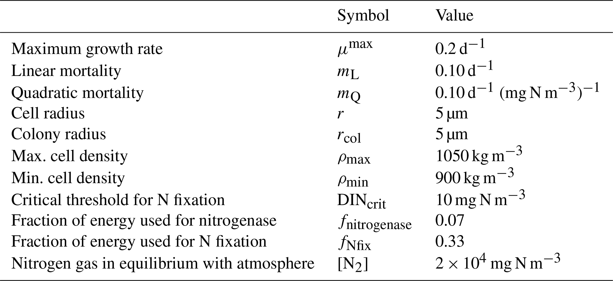
5.2.1 Nitrogen fixation
Nitrogen fixation occurs when the DIN concentration falls below a critical concentration, DINcrit, typically 0.3 to 1.6 µmol L−1 (i.e. 4 to 20 mg N m−3; Robson et al., 2013), at which point Trichodesmium produces nitrogenase to allow fixation of N2. It is assumed that nitrogenase becomes available whenever ambient DIN falls below the value of DINcrit and carbon and phosphorus are available to support nitrogen uptake. The rate of change of internal reserves of nitrogen, RN, due to nitrogen fixation if DIN<DINcrit is given by
where Nfix is the rate of nitrogen fixation per cell and r is the radius of the individual cell. Using this formulation, Trichodesmium is able to maintain its nitrogen uptake rate at that achieved through diffusion-limited uptake at DINcrit even when DIN drops below DINcrit, provided phosphorus and carbon reserves, and , respectively, are available.
The energetic cost of nitrogen fixation is represented as a fixed proportion of carbon fixation, fNfix, equivalent to a reduction in quantum efficiency, and as a proportion, fnitrogenase, of the nitrogen fixed:
where kI is the rate of photon absorption per cell obtain from the microalgal growth model (Table 5).
5.2.2 Buoyancy adjustment
The rate of change of Trichodesmium biomass, B, as a result of density difference between the cell and the water, is approximated by Stokes' law:
where z is the distance in the vertical (positive up), μ is the dynamic viscosity of water, g is acceleration due to gravity, rcol is the equivalent spherical radius of the sinking mass representing a colony radius, ρw is the density of water, and ρ is the cell density given by
where is the normalised carbon reserves of the cell (see above), and ρmin and ρmax are the densities of the cell when there is no carbon reserves and full carbon reserves, respectively. Thus, when light reserves are depleted, the cell is more buoyant, facilitating the retention of Trichodesmium in the surface waters.
5.3 Water column inorganic chemistry
5.3.1 Carbon chemistry
The major pools of dissolved inorganic carbon species in the ocean are , and dissolved CO2, which influence the speciation of H+ and OH− ions, and therefore pH. The interaction of these ions reaches an equilibrium in seawater within a few tens of seconds (Zeebe and Wolf-Gladrow, 2001). In the BGC model here, where calculation time steps are of the order of tens of minutes, it is reasonable to assume that the carbon chemistry system is at equilibrium.
The Ocean Carbon-Cycle Model Intercomparison Project (OCMIP) has developed numerical methods to quantify air–sea carbon fluxes and carbon dioxide system equilibria (Najjar and Orr, 1999). Here, we use a modified version of the OCMIP-2 Fortran code developed for MOM4 (Geophysical Fluid Dynamics Laboratory Modular Ocean Model version 4; Griffies et al., 2004). The OCMIP procedures quantify the state of the carbon dioxide (CO2) system using two prognostic variables, the concentration of dissolved inorganic carbon, DIC, and total alkalinity, AT. The value of these prognostic variables, along with salinity and temperature, are used to calculate the pH and partial pressure of carbon dioxide, pCO2, in the surface waters using a set of governing chemical equations which are solved using a Newton–Raphson method (Najjar and Orr, 1999).
We altered the OCMIP scheme by increasing the search space for the iterative scheme from ±0.5 pH units (appropriate for global models) to ±2.5. With this change, the scheme converges over a broad range of DIC and AT values (Munhoven, 2013). For more details, see Mongin and Baird (2014) and Mongin et al. (2016b).
5.3.2 Nitrification
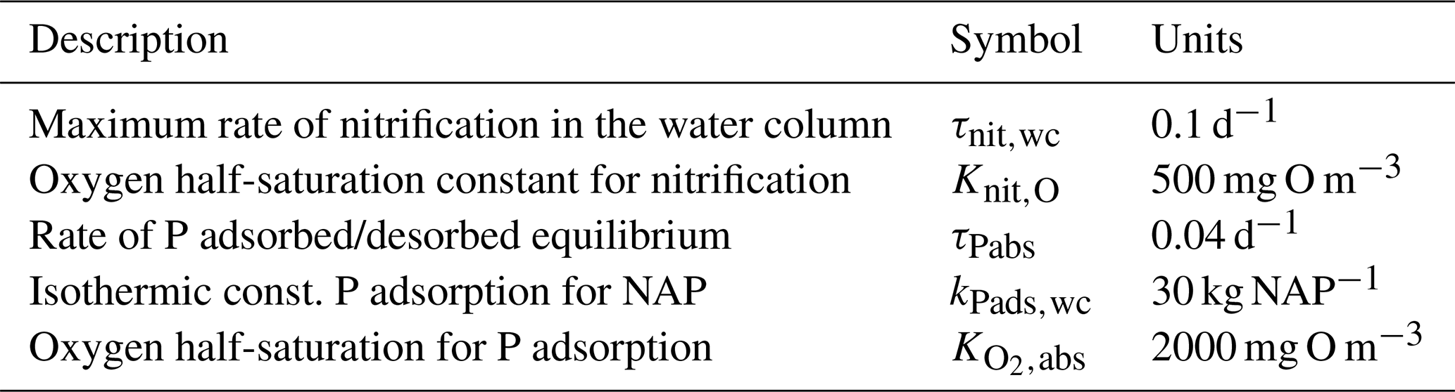
Nitrification is the oxidation of ammonium to form nitrite followed by the rapid oxidation of nitrite to nitrate. This is represented in a one-step process, with the rate of nitrification given by
where the equations and parameter values are defined in Tables 9 and 10.
Table 8State and derived variables for the water column inorganic chemistry model.
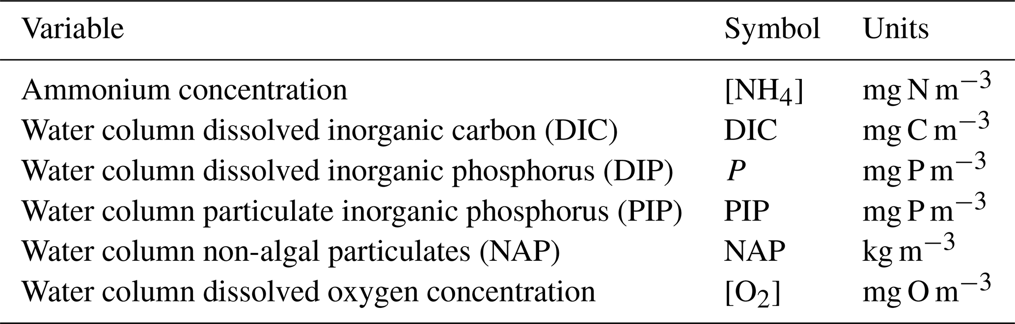
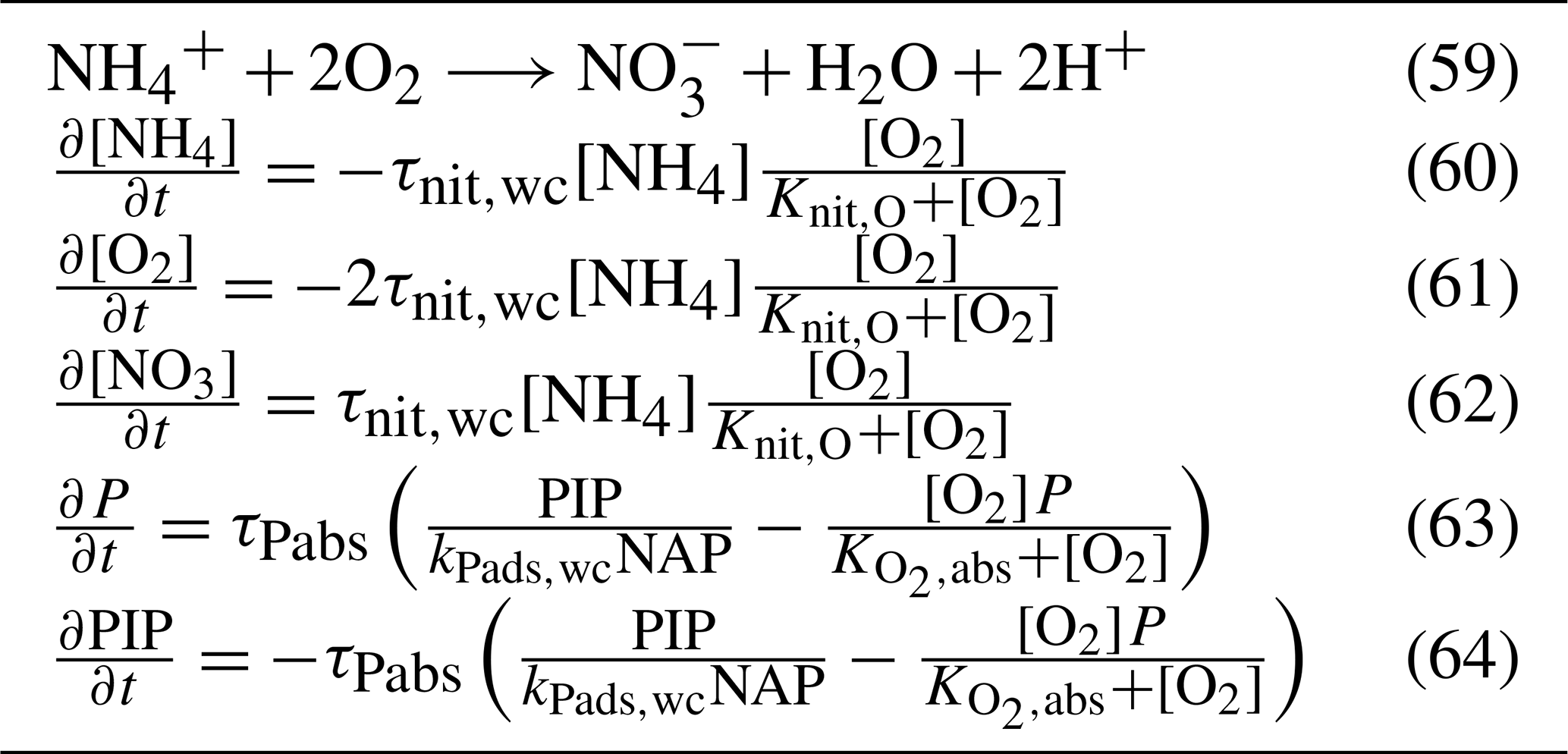
Table 10Constants and parameter values used in the water column inorganic chemistry.
5.3.3 Phosphorus absorption–desorption
The rate of phosphorus desorption from particulates is given by
where [O2] is the concentration of oxygen, P is the concentration of dissolved inorganic phosphorus, PIP is the concentration of particulate inorganic phosphorus, NAP is the sum of the non-algal inorganic particulate concentrations, and τPabs, kPads,wc and are model parameters described in Table 10.
At steady state, the PIP concentration is given by
As an example for rivers flowing into the GBR configuration, [O2]=7411 mg m−3 (90 % saturation at T=25, S=0), NAP =0.231 kg m−3, kg NAP−1, mg O m−3, and P=4.2 mg m−3; thus, the ratio PIP ∕ DIP =6.86 (see Fig. 12). Limited available observations of absorption–desorption include from the Johnstone River (Pailles and Moody, 1992) and the GBR (Monbet et al., 2007).

5.4 Zooplankton herbivory
In the simple food web of the model, herbivory involves small zooplankton consuming small phytoplankton, and large zooplankton consuming large phytoplankton, microphytobenthos and Trichodesmium. For simplicity, the state variables and equations are only given for small plankton grazing (Tables 11, 13), but the parameters are given for all grazing terms (Table 12).
Table 11State and derived variables for the zooplankton grazing. Zooplankton cell mass, mg N cell−1, where VZ is the volume of zooplankton (Hansen et al., 1997).
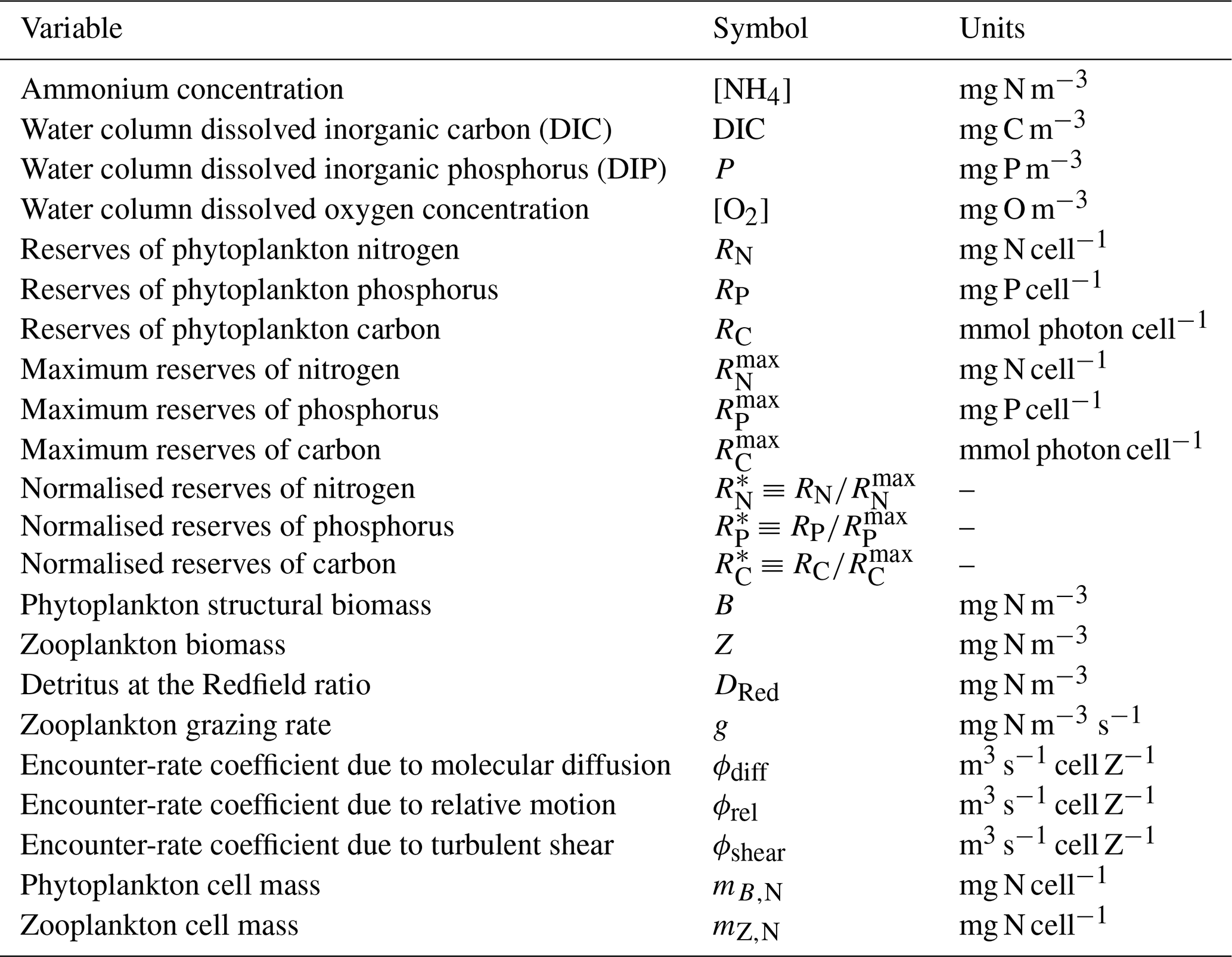
Table 12Constants and parameter values used for zooplankton grazing. Dissipation rate of turbulent kinetic energy (TKE) is considered constant.
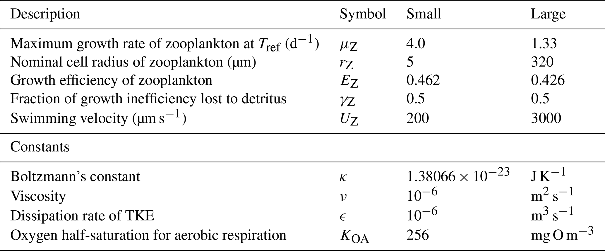
Table 13Equations for zooplankton grazing. The terms represent a predator Z consuming a phytoplankton B. (1) If the zooplankton diet contains multiple phytoplankton classes, and grazing is prey saturated, then phytoplankton loss must be reduced to account for the saturation by other types of microalgae. (2) is the number of individual zooplankton. (3) Phytoplankton pigment is lost to water column without being conserved. Chl a has a chemical formulae of C55H72O5N4Mg and a molecular weight of 893.49 g mol−1. The uptake (and subsequent remineralisation) of molecules for chlorophyll synthesis could make up a maximum (at ) of and , or ∼4 % and ∼2 % of the exchange of C and N between the cell and water column, and will cancel out over the lifetime of a cell. Thus, the error in ignoring chlorophyll loss to the water column is small.
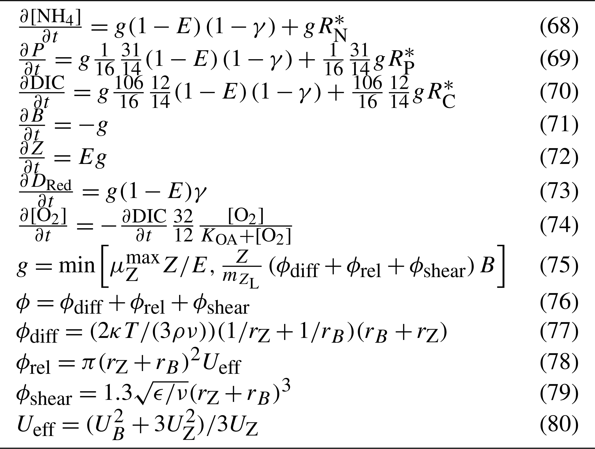
The rate of zooplankton grazing is determined by the encounter rate of the predator and all its prey up until the point at which it saturates the growth of the zooplankton (Eq. 75), and then it is constant. This is a Holling type I grazing response (Gentleman, 2002). Under the condition of multiple prey types, there is no preferential grazing other than that determined by the chance of encounter. The encounter rate is the result of the relative motion of individuals brought about by diffusion (Eq. 77), swimming (Eq. 78) and shear (Eq. 79) determined relative velocities (Eq. 80) (Jackson, 1995; Baird, 2003). One particular advantage of formulating the encounter rate on individuals is that should the number of populations considered in the model change (i.e. an additional phytoplankton class is added), there is no need for empirical coefficients in the model to change. More recent uses of encounter-based grazing functions are described in Flynn and Mitra (2016).
Unlike the microalgae, zooplankton does not contain reserves of nutrients and fixed carbon, and therefore has a fixed stoichiometry of the Redfield ratio. As the zooplankton are grazing on the phytoplankton that contain internal reserves of nutrients, an additional flux of dissolved inorganic nutrients ( for nitrogen) is returned to the water column (for more details, see Sect. 5.4.1).
5.4.1 Conservation of mass in zooplankton grazing
It is important to note that the microalgae model presented above represents internal reserves of nutrients, carbon and chlorophyll as a per cell quantity. Using this representation, there are no losses of internal quantities with either grazing or mortality. However, the implication of their presence is represented in the terms (Table 13) that return the reserves to the water column. These terms represent the fast return of a fraction of phytoplankton nitrogen due to processes like “sloppy eating”.
An alternative and equivalent formulation would be to consider total concentration of microalgal reserves in the water column, then the change in water column concentration of reserves due to mortality (either grazing or natural mortality) must be considered. This alternate representation will not be undertaken here as the above considered equations are fully consistent, but it is worth noting that the numerical solution of the model within the code represents total water column concentrations of internal reserves and therefore must include the appropriate loss terms due to mortality.
5.5 Zooplankton carnivory
Large zooplankton consume small zooplankton. This process uses similar encounter rate and consumption rate limitations calculated for zooplankton herbivory (Table 13). As zooplankton contain no internal reserves, the equations are simplified from the herbivory case to those listed in Table 14. Assuming that the efficiency of herbivory, γ, is equal to that of carnivory, and therefore assigned the same parameter, the additional process of carnivory adds no new parameters to the biogeochemical model.

5.6 Zooplankton respiration
In the model, there is no change in water column oxygen concentration if organic material is exchanged between pools with the same elemental ratio. Thus, when zooplankton consume phytoplankton, no oxygen is consumed due to the consumption of phytoplankton structural material (BP). However, the excess carbon reserves represent a pool of fixed carbon, which when released from the phytoplankton must consume oxygen. Further, zooplankton mortality and growth inefficiency result in detritial production, which when remineralised consumes oxygen. Additionally, carbon released to the dissolved inorganic pool during inefficiency grazing on phytoplankton structural material also consumes oxygen. Thus, zooplankton respiration is implicitly captured in these associated processes.
5.7 Non-grazing plankton mortality
The rate of change of plankton biomass, B, as a result of natural mortality is given by
where mL is the linear mortality coefficient and mQ is the quadratic mortality coefficient.
A combination of linear and quadratic mortality rates are used in the model. When the mortality term is the sole loss term, such as zooplankton in the water column or benthic microalgae in the sediments, a quadratic term is employed to represent increasing predation/viral disease losses in dense populations. For suspended microalgae, we have used only a linear term (i.e. mQ=0). Linear terms have been used to represent a basal respiration rate.
As described in Sect. 5.1.6, the mortality terms need to account for the internal properties of lost microalgae. For definitions of the state variables, see Tables 15 and 16.
Table 15Constants and parameter values used for plankton mortality.
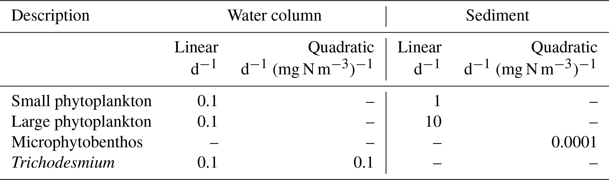
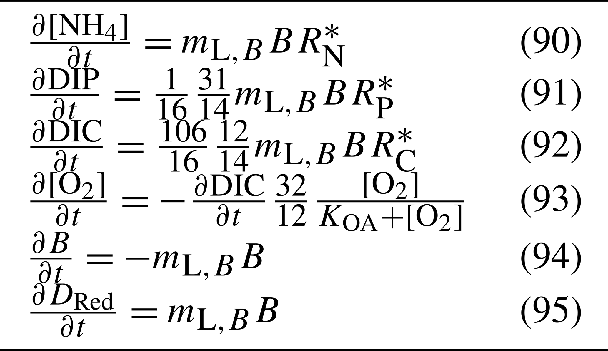
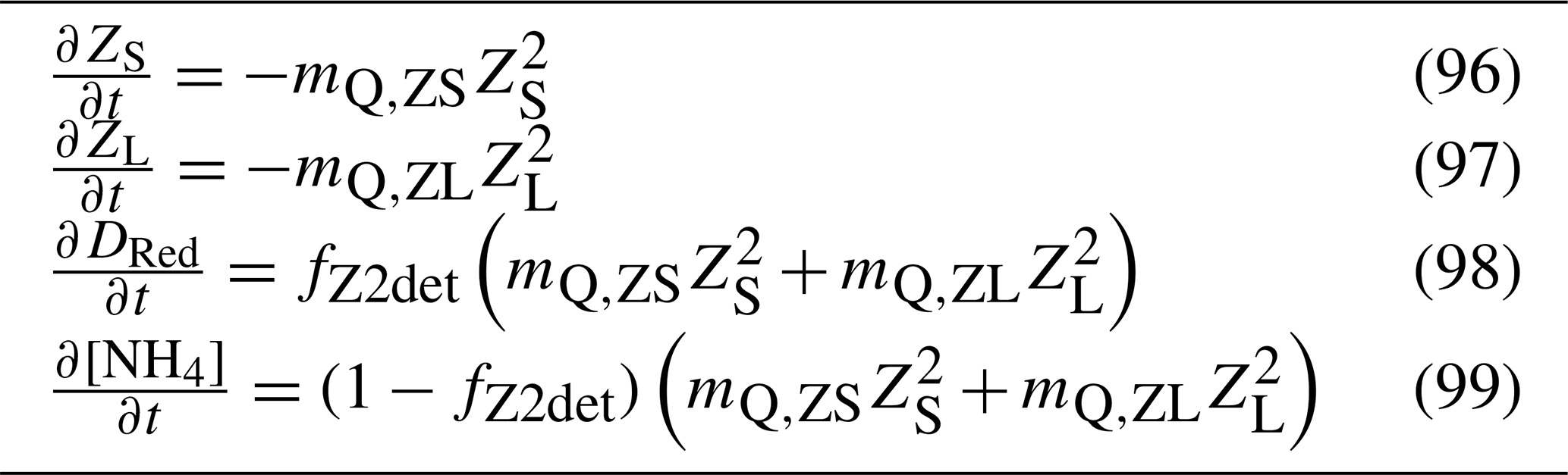
Table 17Equations for the zooplankton mortality. fZ2det is the fraction of zooplankton mortality that is remineralised and is equal to 0.5 for both small and large zooplankton.
5.8 Air–sea gas exchange
Air–sea gas exchange is calculated using wind speed (we choose a cubic relationship; Wanninkhof and McGillis, 1999), saturation state of the gas (described below) and the Schmidt number of the gas (Wanninkhof, 1992). The transfer coefficient, k, is given by
where 0.0283 cm h−1 is an empirically determined constant (Wanninkhof and McGillis, 1999), u10 is the short-term steady wind at 10 m above the sea surface (m s−1), the Schmidt number, Sc, is the ratio of the diffusivity of momentum and that of the exchanging gas, and is given by a cubic temperature relationship (Wanninkhof, 1992). Finally, a conversion factor of 360 000 m s−1 (cm h−1)−1 is used.
In practice, the hydrodynamic model can contain thin surface layers as the surface elevation moves between z levels. Further, physical processes of advection and diffusion and gas fluxes are done sequentially, allowing concentrations to build up through a single time step. To avoid unrealistic changes in the concentration of gases in thin surface layers, the shallowest layer thicker than 20 cm receives all the surface fluxes.
5.8.1 Oxygen
The saturation state of oxygen [O2]sat is determined as a function of temperature and salinity following Weiss (1970). The change in concentration of oxygen in the surface layer due to a sea–air oxygen flux (positive from sea to air) is given by
where is the transfer coefficient for oxygen (Eq. 100), [O2] is the dissolved oxygen concentration in the surface waters, and h is the thickness of the surface layer of the model into which sea–air flux flows.
5.8.2 Carbon dioxide
The change in surface dissolved inorganic carbon concentration, DIC, resulting from the sea–air flux (positive from sea to air) of carbon dioxide is given by
where the transfer coefficient for carbon dioxide (Eq. 100), [CO2] is the dissolved carbon dioxide concentration in the surface waters determined from DIC and AT using the carbon chemistry equilibria calculations described in Sect. 5.3.1, [CO2]atm is the partial pressure of carbon dioxide in the atmosphere, and h is the thickness of the surface layer of the model into which sea–air flux flows.
Note the carbon dioxide flux is determined not by the gradient in DIC but the gradient in [CO2]. At pH values around 8, [CO2] makes up only approximately 1∕200 of DIC in seawater, significantly reducing the air–sea exchange. Counteracting this reduced gradient, note that changing DIC results in an approximately 10-fold change in [CO2] (quantified by the Revelle factor; Zeebe and Wolf-Gladrow, 2001). Thus, the gas exchange of CO2 is approximately of the oxygen flux for the same proportional perturbation in DIC and oxygen. At a Sc number of 524 (25 ∘C seawater) and a wind speed of 12 m s−1, 1 m of water equilibrates with CO2 in the atmosphere with an e-folding timescale of approximately 1 d.
In the model, benthic communities are quantified as a biomass per unit area or areal biomass. At low biomass, the community is composed of a few specimens spread over a small fraction of the bottom, with no interaction between the nutrient and energy acquisition of individuals. Thus, at low biomass, the areal fluxes are a linear function of the biomass.
As biomass increases, the individuals begin to cover a significant fraction of the bottom. For nutrient and light fluxes that are constant per unit area, such as downwelling irradiance and sediment releases, the flux per unit biomass decreases with increasing biomass. Some processes, such as photosynthesis in a thick seagrass meadow or nutrient uptake by a coral reef, become independent of biomass (Atkinson, 1992) as the bottom becomes completely covered. To capture the non-linear effect of biomass on benthic processes, we use an effective projected area fraction, Aeff.
To restate, at low biomass, the area on the bottom covered by the benthic community is a linear function of biomass. As the total leaf area approaches and exceeds the projected area, the projected area for the calculation of water-community exchange approaches 1 and becomes independent of biomass. This is represented using
where Aeff is the effective projected area fraction of the benthic community (m2 m−2), B is the biomass of the benthic community (g N m−2), and ΩB is the nitrogen-specific leaf area coefficient (m2 g N−1). For further explanation of ΩB, see Baird et al. (2016a).
The parameter ΩB is critical: it provides a means of converting between biomass and fractions of the bottom covered and is used in calculating the absorption cross-section of the leaf and the nutrient uptake of corals and macroalgae. That ΩB has a simple physical explanation and can be determined from commonly undertaken morphological measurement (see below), gives us confidence in its use throughout the model.
6.1 Macroalgae
The macroalgae model considers the diffusion-limited supply of dissolved inorganic nutrients (N and P) and the absorption of light, delivering N, P and fixed C, respectively. Unlike the microalgae model, no internal reserves are considered, implying that the macroalgae has a fixed stoichiometry that can be specified as
where the stoichiometry is based on Atkinson and Smith (1983) (see also Baird and Middleton, 2004; Hadley et al., 2015a, b). Note that when ammonium is taken up instead of nitrate there is a slightly different O2 balance (Sect. 9.1). In the next section, we will consider the maximum nutrient uptake and light absorption and then bring them together to determine the realised growth rate.
6.1.1 Nutrient uptake
Nutrient uptake by macroalgae is a function of nutrient concentration, water motion (Hurd, 2000) and internal physiology. The maximum flux of nutrients is specified as a mass transfer limit per projected area of macroalgae and is given by (Falter et al., 2004; Zhang et al., 2011)
where Sx is the mass transfer rate coefficient of element x= N, P, τ is the shear stress on the bottom, ρ is the density of water, and Scx is the Schmidt number. The Schmidt number is the ratio of the diffusivity of momentum, ν, and mass, Dx (Table 6), and varies with temperature, salinity and nutrient species. The rate constant S can be thought of as the height of water cleared of mass per unit of time by the water–macroalgae exchange.
6.1.2 Light capture
The calculation of light capture by macroalgae involves estimating the fraction of light that is incident upon the leaves and the fraction that is absorbed. The rate of photon capture is given by
where h, c and AV are fundamental constants, 109 nm m−1 accounts for the typical representation of wavelength, λ, in nm, and AL,λ is the spectrally resolved leaf-specific absorptance. As shown in Eq. (103), the term gives the effective projected area fraction of the community. In the case of light absorption of macroalgae, the exponent is multiplied by the leaf-specific absorptance, AL,λ, to account for the transparency of the leaves. At low macroalgae biomass, absorption at wavelength λ is equal to , increasing linearly with biomass as all leaves at low biomass are exposed to full light (i.e. there is no self-shading). At high biomass, the absorption by the community asymptotes to Ed,λ, at which point increasing biomass does not increase the absorption as all light is already absorbed.
For more details on the calculation of ΩMA, see Baird et al. (2016a).
6.1.3 Growth
The growth rate combines nutrient, light and maximum organic matter synthesis rates following
and the production of macroalgae is given by μMAMA. We have used the commonly applied multiple minimum function (von Liebig, 1840), although it is noted that others use the multiple of limitation terms (Fasham, 1993). The microalgae model described above uses dynamical reserves to determine the growth rate. The growth approximated using dynamical reserves closer approximates a multiple minimum function than a multiple of minimum terms, so it was deemed more appropriate to use a multiple minimum function for macroalgae and seagrass for which internal reserves were not resolved.
The maximum growth rate is inside the minimum operator. This allows the growth of macroalgae to be independent of temperature at low light but still have an exponential dependence at maximum growth rates (Baird et al., 2003).
6.1.4 Mortality
Mortality is defined as a simple linear function of biomass:
A quadratic formulation is not necessary as both the nutrient and light capture rates become independent of biomass as . Thus, the steady-state biomass of macroalgae under nutrient limitation is given by
and for light-limited growth by
The full macroalgae variables, equations and parameters are listed in Tables 18, 19 and 20.
Table 18State and derived variables for the macroalgae model. For simplicity, in the equations, all dissolved constituents are given in grams, although elsewhere they are shown in milligrams.
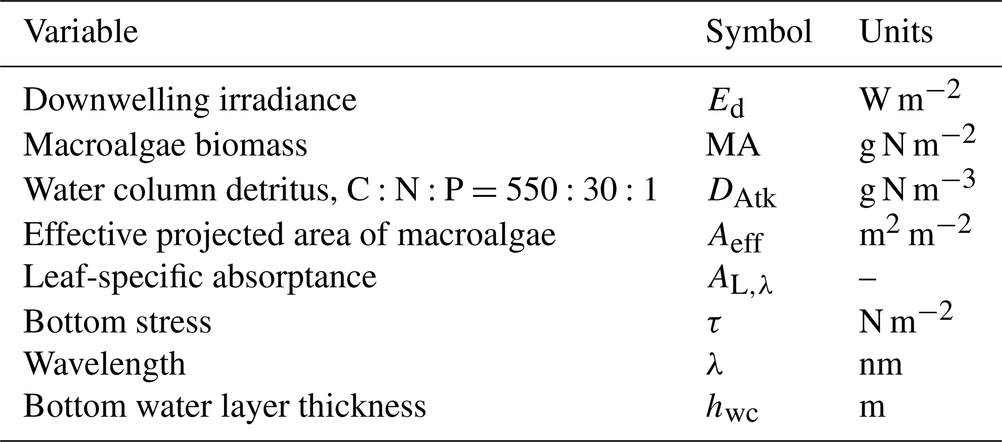
Table 19Equations for the macroalgae model. Other constants and parameters are defined in Table 20: 14 g N mol N−1; 12 g C mol C−1; 31 g P mol P−1; 32 g O mol O2−1. Uptake shown here is for nitrate; see Sect. 9.1 for ammonium uptake.
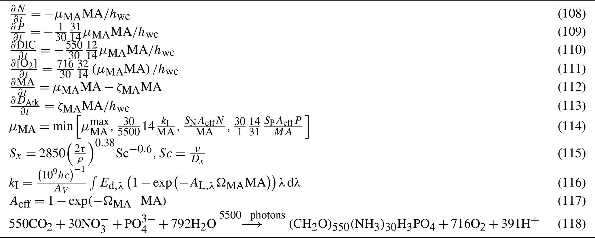
Table 20Constants and parameter values used to model macroalgae.
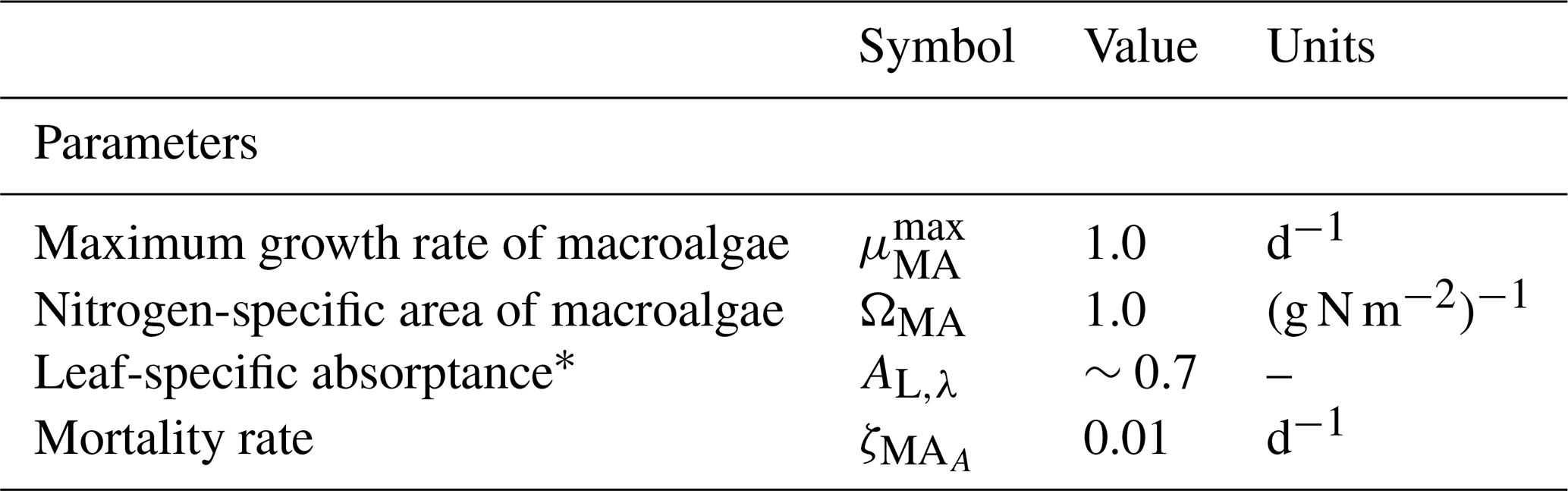
* Spectrally resolved values.
6.2 Seagrass
Seagrasses are quantified per m2 with a constant stoichiometry () for both above-ground, SGA, and below-ground, SGB, biomass and can translocate organic matter at this constant stoichiometry between the two stores of biomass. Growth occurs only in the above-ground biomass, but losses (grazing, decay, etc.) occur in both. Multiple seagrass varieties are represented. The varieties are modelled using the same equations for growth, respiration and mortality but with different parameter values. Here, we just list the variables, equations and parameters (Tables 21, 22 and 23) for the seagrass submodel. A description of the seagrass processes of growth, translocation between roots and leaves, and mortality has been published in Baird et al. (2016a), along with a comparison to observations from Gladstone Harbour on the northeast Australian coast.
Table 21State and derived variables for the seagrass model. For simplicity, in the equations, all dissolved constituents are given in grams, although elsewhere they are shown in milligrams. The bottom water column thickness is spatially variable depending on bathymetry.
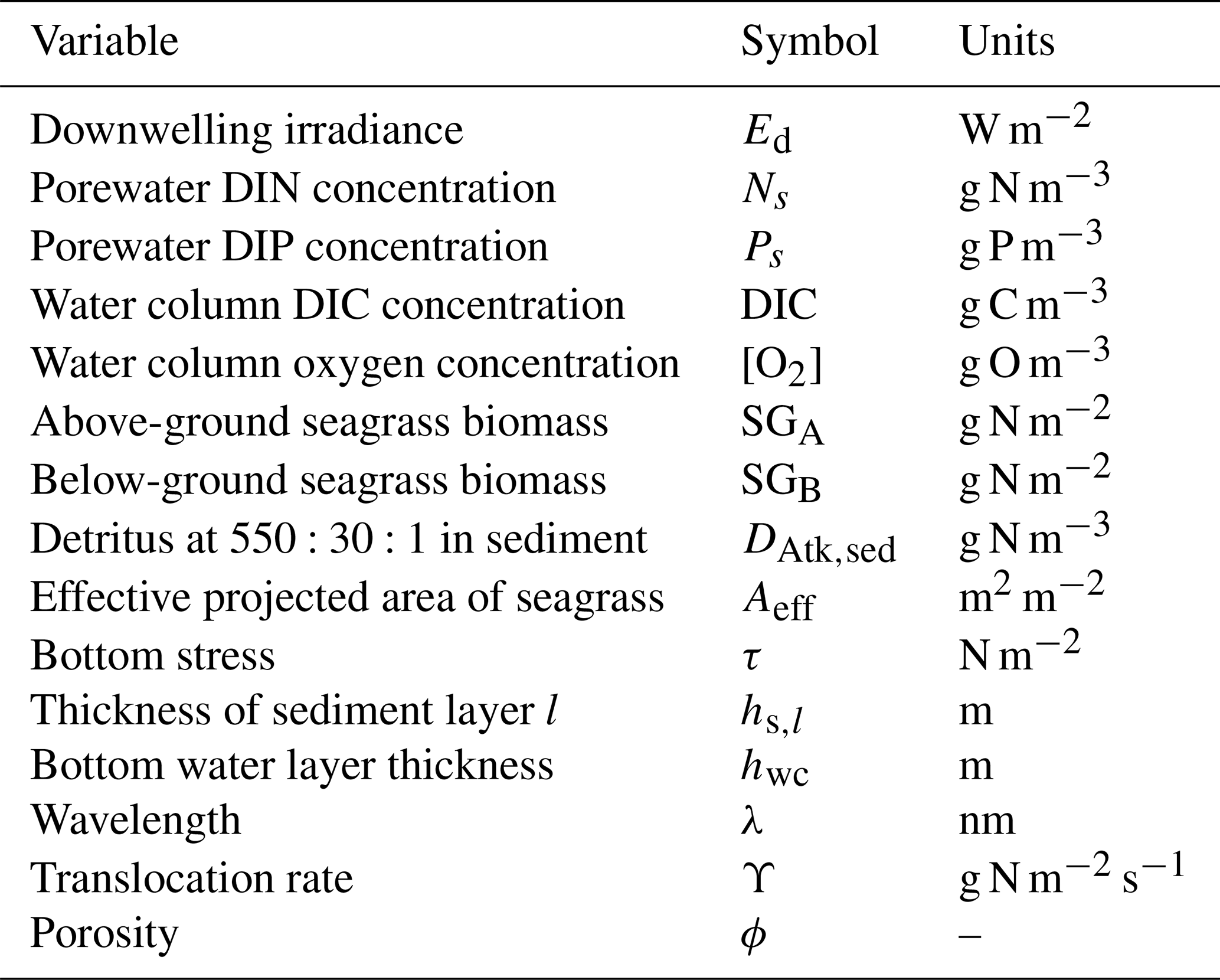
Table 22Equations for the seagrass model. Other constants and parameters are defined in Table 23. The equation for organic matter formation gives the stoichiometric constants; 14 g N mol N−1; 12 g C mol C−1; 31 g P mol P−1; 32 g O mol O2−1.
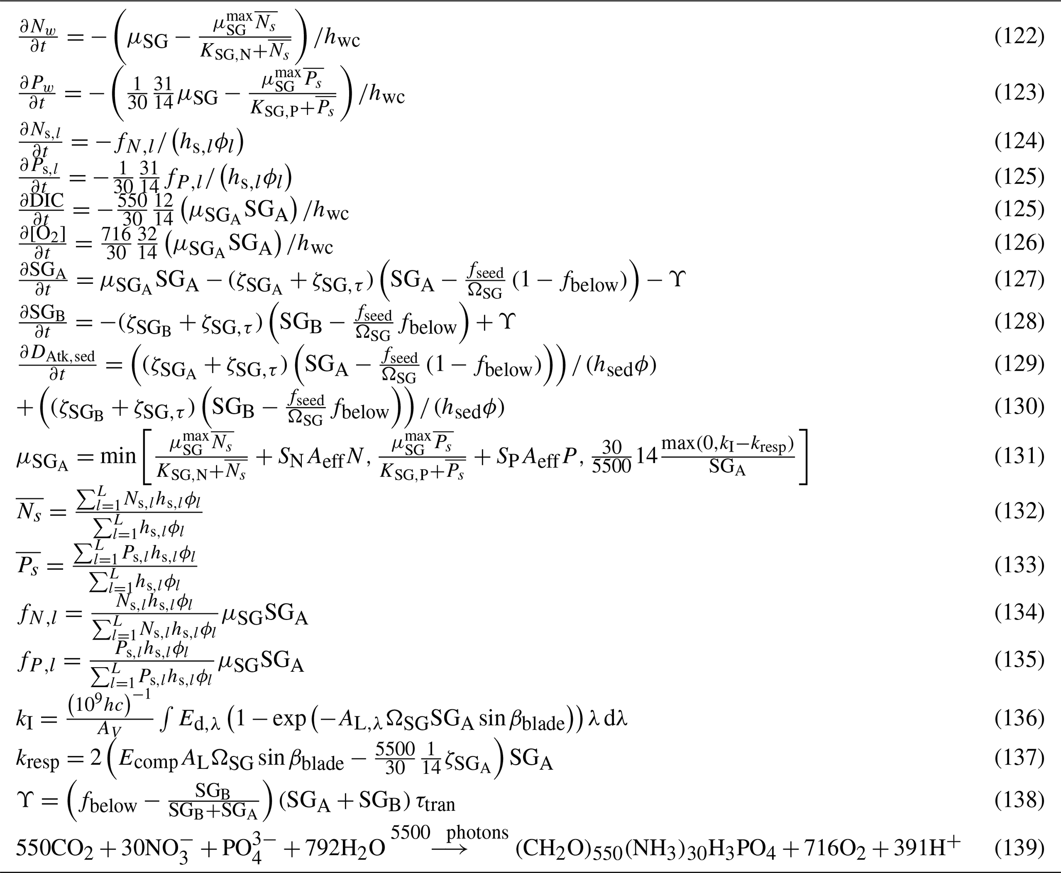
Table 23Constants and parameter values used to model seagrass. a Factor of 2 for nighttime, factor of 2 for roots. b Zostera is calculated from leaf characteristics in Kemp et al. (1987); Hansen et al. (2000); Halophila ovalis is calculated from leaf dimensions in Vermaat et al. (1995); ΩSG can also be determined from specific leaf area such as determined in Cambridge and Lambers (1998) for nine Australian seagrass species. c Spectrally resolved values in Baird et al. (2016a). d Duarte and Chiscano (1999). e Loosely based on Kaldy et al. (2013). f Thalassia testudinum (Gras et al., 2003). g Thalassia testudinum (Lee and Dunton, 1999). h Chartrand et al. (2012); Longstaff (2003); Chartrand et al. (2017). i Roberts (1993).

6.3 Coral polyps
The coral polyp parameterisation consists of a microalgae growth model to represent zooxanthellae growth based on Baird et al. (2013), and the parameterisation of coral–zooxanthellae interaction based on the host–symbiont model of Gustafsson et al. (2013), and the photo-adaptation, photo-inhibition and reaction centre dynamics model of Baird et al. (2018). The extra detail on the zooxanthellae photosystem is required due to its important role in thermal-stress-driven coral bleaching (Yonge, 1930; Suggett et al., 2008).
6.3.1 Coral host, symbiont and the environment
The state variables for the coral polyp model (Table 24) include the biomass of coral tissue, CH (g N m−2), and the structure material of the zooxanthellae cells, CS (mg N m−2). The structure material of the zooxanthellae, CS, in addition to nitrogen, contains carbon and phosphorus at the Redfield ratio. The zooxanthellae cells also contain reserves of nitrogen, RN (mg N m−2), phosphorus, RP (mg P m−2), and carbon, RC (mg C m−2).
Table 24Model state variables for the coral polyp model. Note that water column variables are three-dimensional, benthic variables are two-dimensional, and unnormalised reserves are per cell.
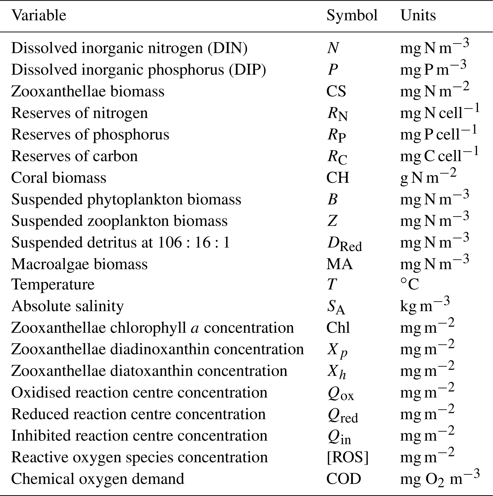
The zooxanthellae light absorption capability is resolved by considering the time-varying concentrations of pigments chlorophyll a, Chl, diadinoxanthin, Xp, and diatoxanthin, Xh, for which the state variable represents the areal concentration. A further three pigments, chlorophyll c2, peridinin and β carotene, are considered in the absorption calculations, but their concentrations are in fixed ratios to chlorophyll a. Exchanges between the coral community and the overlying water can alter the water column concentrations of dissolved inorganic carbon, DIC, nitrogen, N, and phosphorus, P, as well as particulate phytoplankton, B, zooplankton, Z, and detritus, D, where multiple nitrogen, plankton and detritus types are resolved (Table 24).
The coral host is able to assimilate particulate organic nitrogen either through translocation from the zooxanthellae cells or through the capture of water column organic detritus and/or plankton. The zooxanthellae varies its intracellular pigment content depending on potential light limitation of growth, and the incremental benefit of adding pigment, allowing for the package effect (Baird et al., 2013). The coral tissue is assumed to have a Redfield stoichiometry (Redfield et al., 1963), as shown by Muller-Parker et al. (1994). The zooxanthellae are modelled with variable ratios (Muller-Parker et al., 1994), based on a structure material at the Redfield ratio but with variable internal reserves. The fluxes of C, N and P with the overlying water column (nutrient uptake and detritial/mucus release) can therefore vary from the Redfield ratio.
Here, we present the state variables (Table 24), derived variables (Table 25), equations (Tables 26, 27, 28 and 29) and parameters values (Tables 30 and 31) for the coral submodel. The description of the coral processes has been published in Baird et al. (2018), along with a comparison to observations from the Great Barrier Reef on the northeast Australian coast.
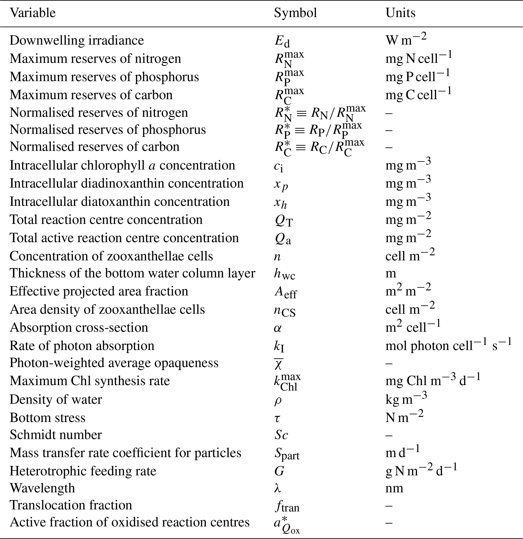
Table 26Equations for the interactions of coral host, symbiont and environment excluding bleaching loss terms that appear in Table 29. The term is the concentration of zooxanthellae cells. The equation for organic matter formation gives the stoichiometric constants; 12 g C mol C−1; 32 g O mol O2−1.
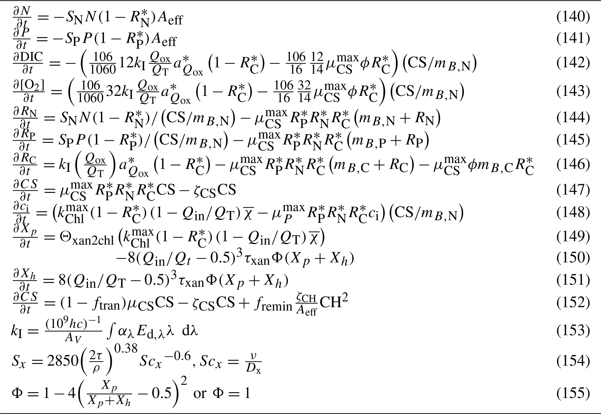
Table 27Equations for the coral polyp model. The term is the concentration of zooxanthellae cells. The equation for organic matter formation gives the stoichiometric constants; 12 g C mol C−1; 32 g O mol O2−1. Other constants and parameters are defined in Table 31.
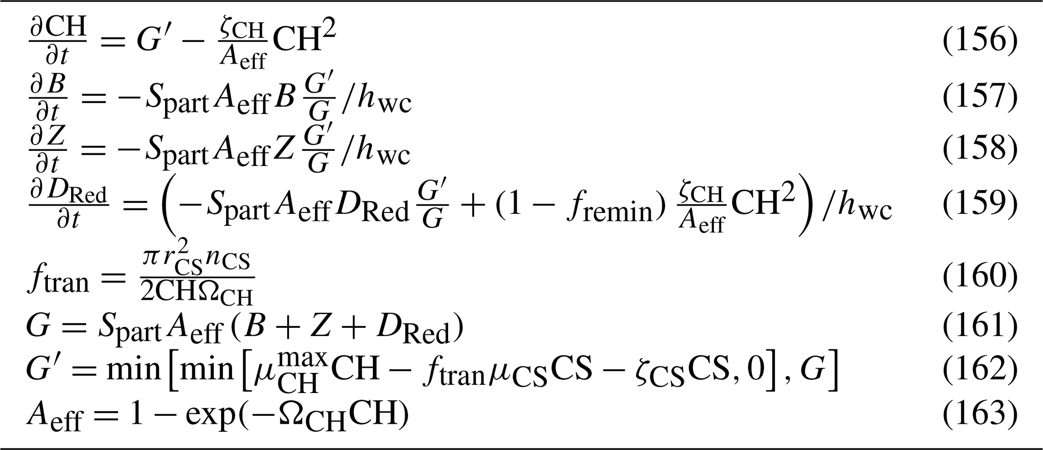
Table 28Equations for symbiont reaction centre dynamics. Bleaching loss terms appear in Table 29.

Table 29Equations describing the expulsion of zooxanthellae and the resulting release of inorganic and organic molecules into the bottom water column layer.
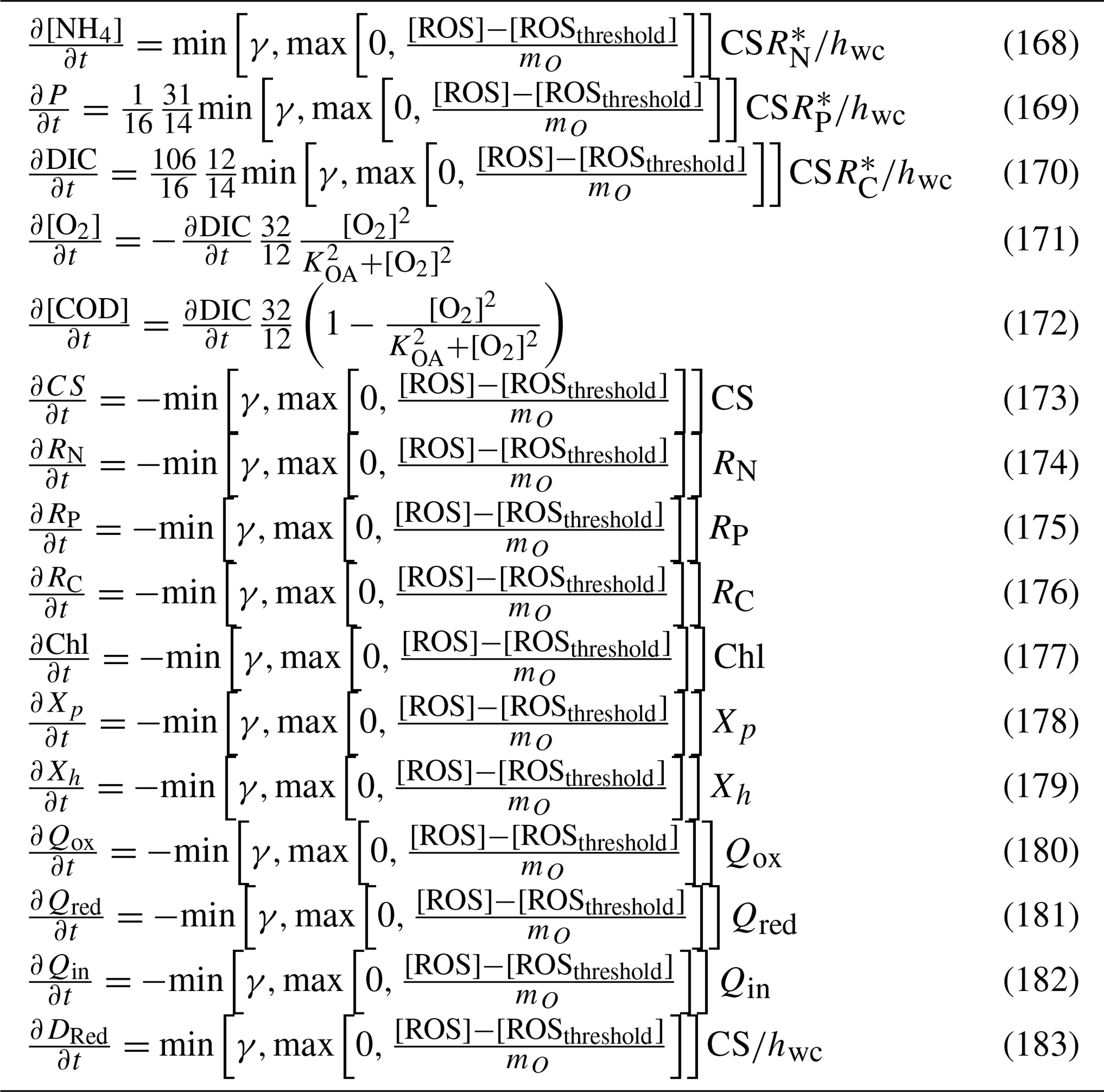
Table 30Constants and parameter values used to model coral polyps. V is zooxanthellae cell volume in µm3.
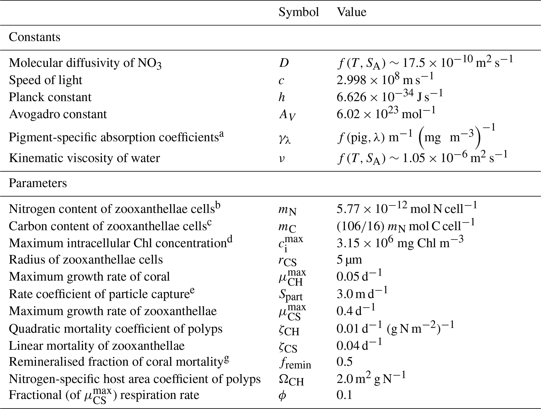
a Baird et al. (2016a). b Straile (1997). c Redfield et al. (1963) and Kirk (1994). d Finkel (2001). e Ribes and Atkinson (2007); Wyatt et al. (2010). f, g Gustafsson et al. (2013, 2014).
Table 31Constants and parameter values used in the coral bleaching model. “RCII” indicates the reaction centre of photosystem II.
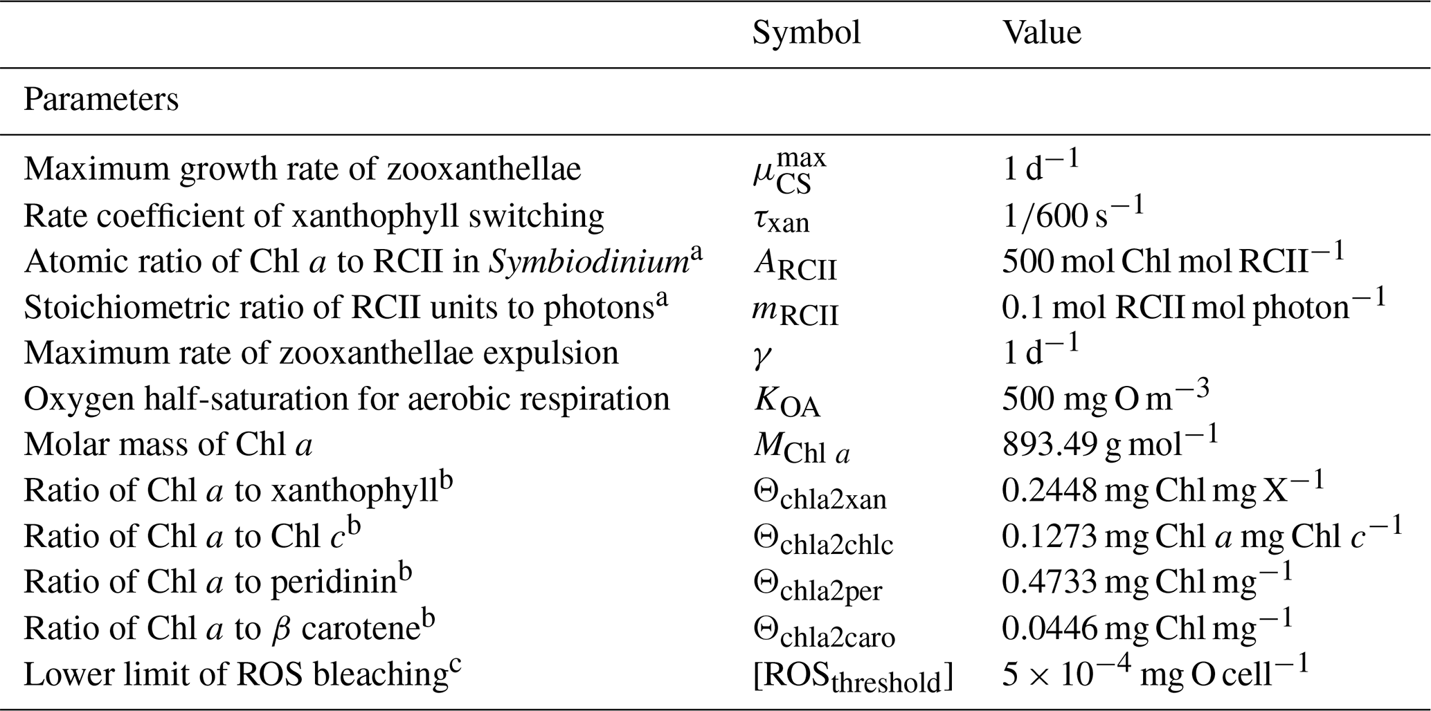
a In Suggett et al. (2009). b Ratio of constant terms in multivariate analysis in Hochberg et al. (2006). c Fitted parameter based on the existence of non-bleaching threshold (Suggett et al., 2009) and a comparison of observed bleaching and model output in the ∼1 km model.
6.3.2 Coral calcification
The rate of coral calcification is a function of the water column aragonite saturation, Ωa, and the normalised reserves of fixed carbon in the symbiont, . The rates of change of DIC and total alkalinity, AT, in the bottom water column layer of thickness hwc due to calcification becomes
where g is the rate of net calcification, kday and knight are defined in Table 30 with habitat-specific values (Anthony et al., 2011; Mongin and Baird, 2014). The fluxes are scaled by the effective projected area of the community, Aeff. The power of 2 for ensures that generally light-replete symbionts provide the host with sufficient energy for calcification.
Table 32Equations for coral polyp calcification and dissolution. The concentration of carbonate ions, , is determined from equilibrium carbon chemistry as a function of AT, DIC, temperature and salinity, and the concentration of calcium ions, [Ca2+], is a mean oceanic value; 12 g C mol C−1. Other constants and parameters are defined in Table 30.
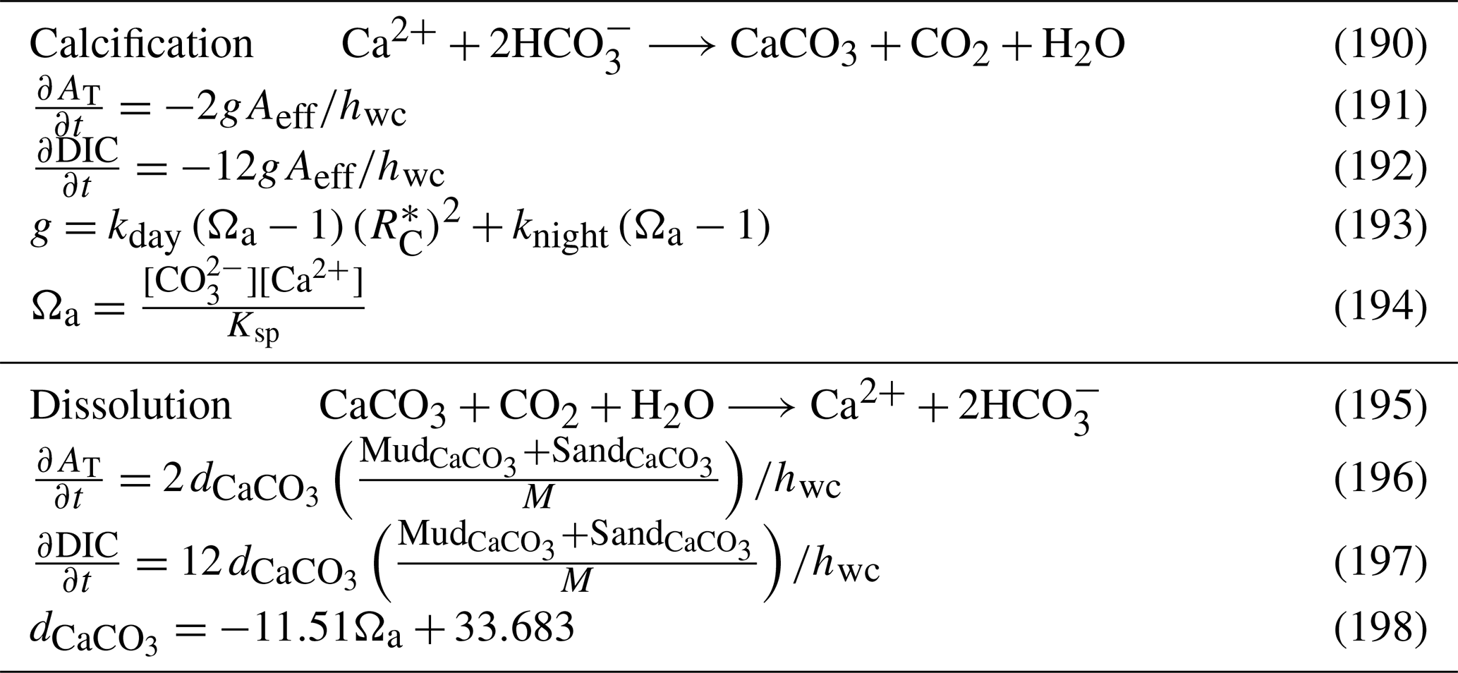
6.3.3 Dissolution of shelf carbonate sands
In addition to the dissolution of carbonate sands on a growing coral reef, which is captured in the net dissolution quantified above, the marine carbonates on the continental shelf dissolve (Eyre et al., 2018). Like above, the dissolution of marine carbonates is approximated as a source of DIC and alkalinity but does not affect the properties (mass, porosity, etc.) of the underlying sediments.
We assume carbonate dissolution from the sediment bed is proportional to the fraction of the total surface sediment that is composed of either sand or mud carbonates. Other components, whose fraction do not release DIC and alkalinity, include carbonate gravel and non-carbonate mineralogies. Thus, the change in DIC and AT in the bottom water column layer is given by
where M is the total mass of surface layer inorganic sediments (see Sect. 7), is the dissolution rate of CaCO3 and is the reverse reaction to calcification, and hwc is the thickness of the water column layer. The dissolution rate, (mmol m−2 d−1), is assumed to be a function of Ωa (Eyre et al., 2018):
7.1 Brief summary of processes in the sediments
The EMS model contains a multi-layered sediment compartment with time- and space-varying vertical layers and the same horizontal grid as the water column and epibenthic models. All state variables that exist in the water column layers have an equivalent in the sediment layers. The dissolved tracers are given as a concentration in the porewater, while the particulate tracers are given as a concentration per unit volume (see Sect. 10.3.2).
The sediment model contains inorganic particles of different sizes (dust, mud, sand and gravel) and different mineralogies (carbonate and non-carbonate) (Table 33). The sediment model includes the processes of particulate advection and mixing in the water column, resuspension sinking and settling, as well as sediment overturning and bioturbation (Margvelashvili, 2009). These processes, along with initial conditions, determine the mass of each inorganic particulate type in the sediments.
Table 33Characteristics of the particulate classes. Y – yes, N – no, I – initial condition, C – catchment, OM – remineralisation from organic matter, B – brown, W – white (Condie et al., 2009; Margvelashvili, 2009).
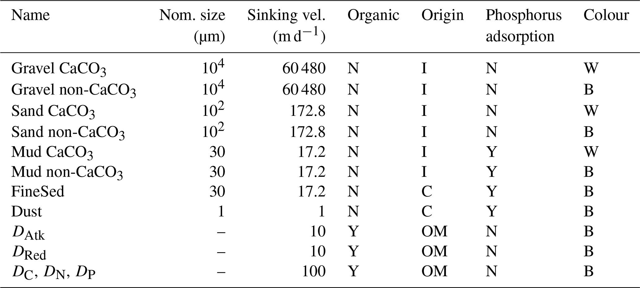
The critical shear stress for resuspension and the sinking rates are generally larger for large particles, while mineralogy only affects the optical properties. The size-class dust only has a non-carbonate form. FineSed also only has a non-carbonate form and has the same physical and optical properties as non-carbonate mud, except that it is initialised with a zero value. Dust and FineSed are particles that enter the domain from rivers during the simulation.
The organic matter classes are discussed in the Sect. 8.1. The inorganic and organic particulate classes are summarised in Table 33 and undergo resuspension, sinking, settling, sediment overturning and bioturbation in a manner similar to the inorganic particulates.
7.2 Sediment chemistry
7.2.1 Sediment nitrification–denitrification
Nitrification in the sediment is similar to the water column but with a sigmoid rather than hyperbolic relationship at low oxygen for numerical reasons (Eq. 204). Denitrification occurs only in the sediment.
7.2.2 Sediment phosphorus absorption–desorption
Sediment phosphorus absorption–desorption is similar to water column (Eq. 206). There is an additional pool of immobilised particulate inorganic phosphorus (PIPI) which accumulates in the model over time as PIP becomes immobilised and represents permanent sequestration (Eq. 207).
8.1 Detritus remineralisation
The non-living components of the C, N and P cycles include the particulate labile and refractory pools, and a dissolved pool (Fig. 4). The labile detritus has a pool at the Redfield ratio, DRed, and at the Atkinson ratio, DAtk, resulting from mortality of organic matter at these ratios (see processes above). The labile detritus from both pools then breaks down into refractory detritus and dissolved organic matter. In order to account for the mixed source of labile detritus, the refractory detritus and dissolved organic matter pools are quantified by individual elements (C, N, P). A component of the breakdown of each of these pools is returned to dissolved inorganic components. Finally, as the refractory and dissolved components are separated into C, N and P components, this introduces the possibility to have P components break down quicker than C and N. This is specified as the breakdown rate of P relative to N, and , respectively, for refractory and dissolved detritus. The variables, equations and parameter values for detritus remineralisation can be found in Tables 37, 38 and 39, respectively.
Table 34State and derived variables for the sediment inorganic chemistry model.
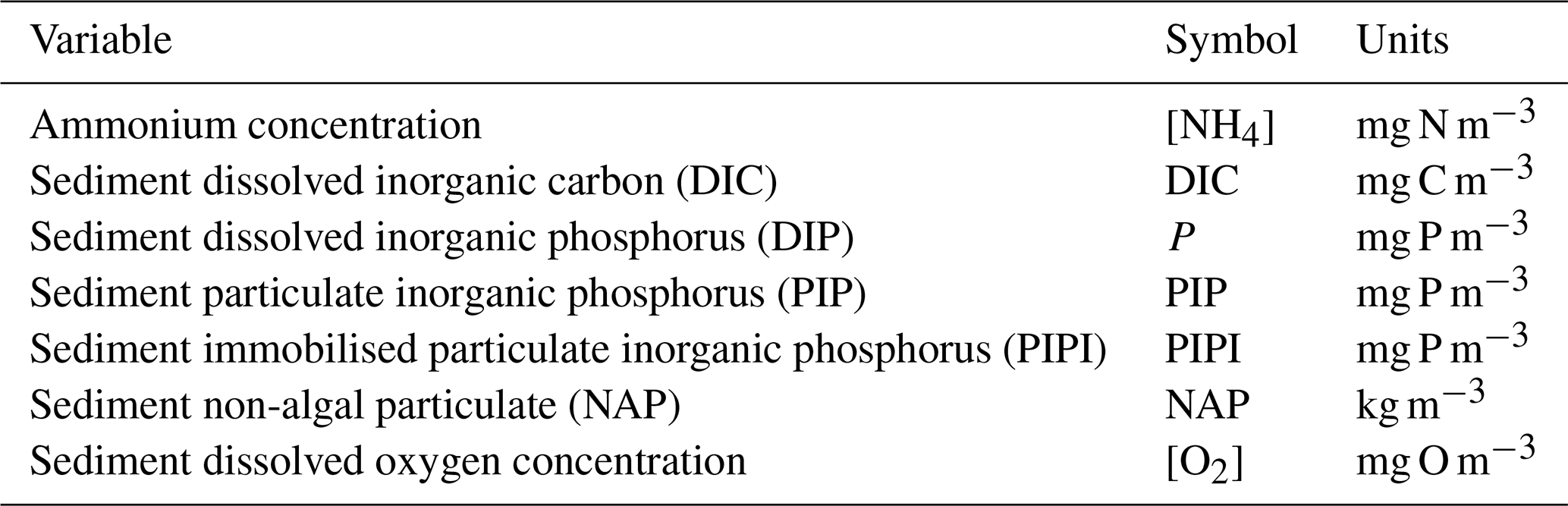
Table 35Constants and parameter values used in the sediment inorganic chemistry.
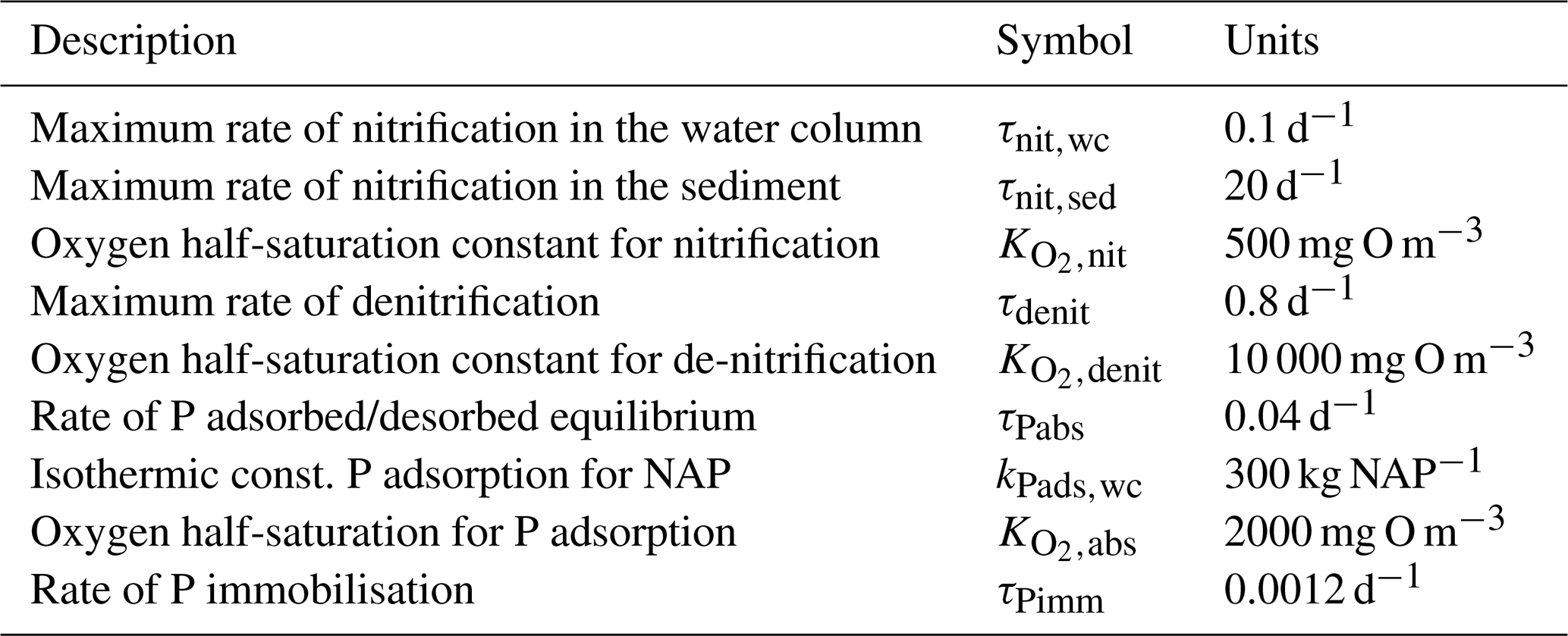
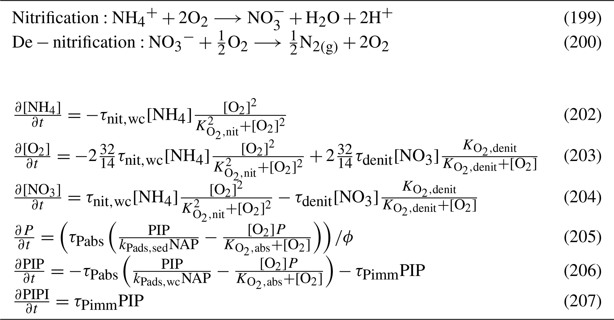
Table 37State and derived variables for the detritus remineralisation model in both the sediment and water column.
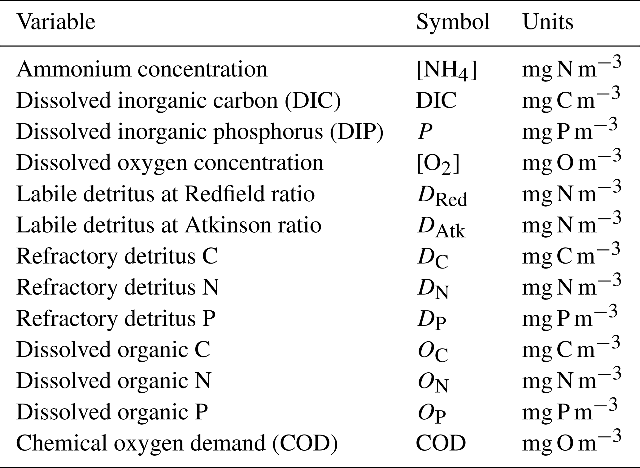
Table 38Equations for detritus remineralisation in the water column and sediment.
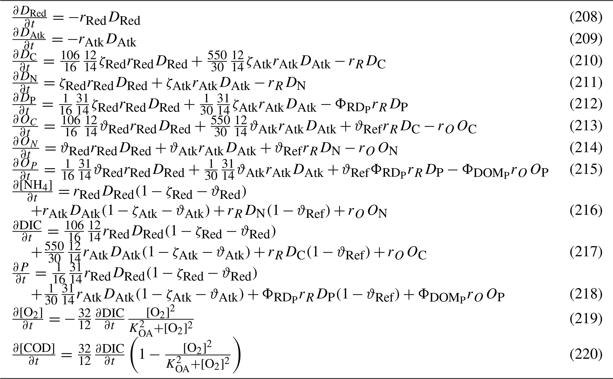
Table 39Constants and parameter values used in the water column detritus remineralisation model. Red is the Redfield ratio (); Atk is the Atkinson ratio (); see Lønborg et al. (2017). n/a – not applicable
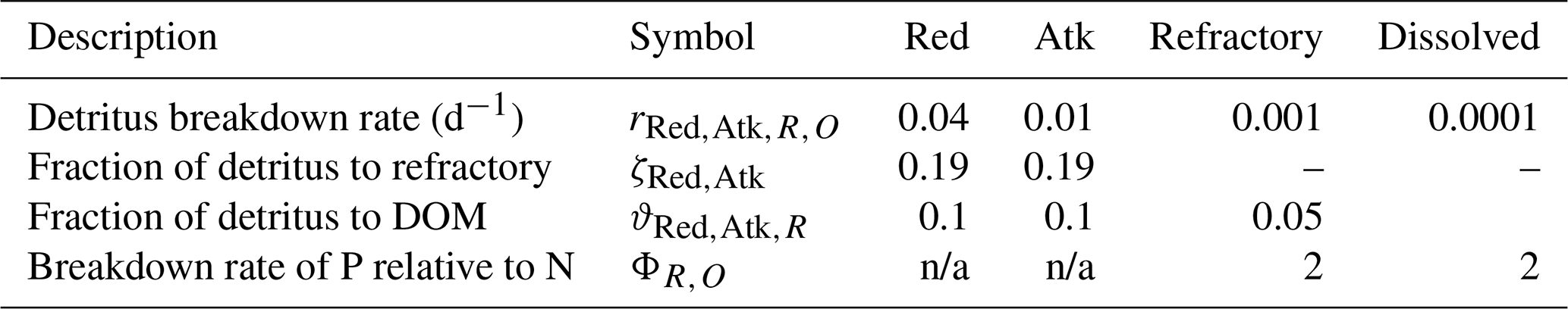
8.1.1 Anaerobic and anoxic respiration
The processes of remineralisation, phytoplankton mortality and zooplankton grazing return carbon dioxide to the water column. In oxic conditions, these processes consume oxygen in a ratio of DIC : . At low oxygen concentrations, the oxygen consumed is
where KOA is the half-saturation constant for anoxic respiration (Boudreau, 1996). A sigmoid saturation term is used because it is more numerically stable as the oxygen concentration approaches 0. The anoxic component of remineralisation results in an increased chemical oxygen demand (COD):
where COD is a dissolved tracer, with the same units as oxygen.
When oxygen and COD coexist, they react to reduce both, following
where 8000 mg O m−3 is approximately the saturation concentration of oxygen in seawater, and τCOD is the timescale of this reduction. The term min[COD,8000] is required because COD represents the end stage of anoxic reduction and can become large for long simulations. Even with this limitation, if τCOD=1 h−1, the processes in Eqs. (223) and (224) proceed faster than most of the other porewater processes.
Most of the ecological processes contain a temperature dependence and, for those uptaking dissolved inorganic nitrogen, preferential ammonium uptake. To simplify the description of the above processes, these common parameterisations are described separately in this section. An additional processes common to all variables, and across multiples zones, is the diffusive sediment–water exchange.
9.1 Preferential uptake of ammonium
The model contains two forms of dissolved inorganic nitrogen (DIN) used by photosynthetic organisms, dissolved ammonium (NH4) and dissolved nitrate (NO3):
where N is the concentration of DIN, [NH4] is the concentration of dissolved ammonium and [NO3] is the concentration of nitrate. In the model, the ammonium component of the DIN pool is assumed to be taken up first, followed by the nitrate, with the caveat that the uptake of ammonium cannot exceed the diffusion limit for ammonium. The underlying principle of this assumption is that photosynthetic organisms can entirely prefer ammonium but that the uptake of ammonium is still limited by diffusion to the organism's surface.
As the nitrogen uptake formulation varies for the different autotrophs, the formulation of the preference of ammonium also varies. The diffusion coefficient of ammonium and nitrate are only 3 % different, so for simplicity we have used the nitrate diffusion coefficient for both.
Thus, for microalgae (Eq. 40) and Trichodesmium (Eq. 55), which both contain internal reserves of nitrogen, the partitioning of nitrogen uptake is given by
For macroalgae (Eq. 108) and seagrass leaves (Eq. 122), which also have diffusion limits to uptake but are not represented with internal reserves of nitrogen, the terms are
Zooxanthellae is a combination of the two cases above, because in the model they contain reserves like microalgae, but the uptake rate is across a 2-D surface like macroalgae.
In the case of nutrient uptake by seagrass roots (Eq. 124), which has a saturating nitrogen uptake functional form, the terms are
where KN is a function of the ratio of above-ground to below-ground biomass described in Baird et al. (2016a).
One feature worth noting is that the above formulation for preferential ammonium uptake requires no additional parameters, which is different to other classically applied formulations (Fasham et al., 1990) that require a new parameter, potentially for each autotroph. This simple use of the geometric constraint has an important role in reducing model complexity.
9.2 Oxygen release during nitrate uptake
For all autotrophs, the uptake of a nitrate ion results in the retention of the one nitrogen atom in their reserves or structural material, and the release of the three oxygen atoms into the water column or porewaters.
The oxygen that is part of the structural material of microalgae is assumed to have been taken up through photosynthesis.
For simplicity, in the equations for autotroph-driven changes in dissolved oxygen above, we have assumed that DIN uptake is ammonium. Thus, after partitioning on nitrogen uptake, the term in Eq. (235) needs to be added to change in oxygen in microalgae (Eq. 40), Trichodesmium (Eq. 55) and other autotrophs.
9.3 Temperature dependence of ecological rates
Physiological rate parameters (maximum growth rates, mortality rates, remineralisation rates) have a temperature dependence that is determined from
where rT is the physiological rate parameter (e.g. μ, ζ) at temperature T, Tref is the reference temperature (nominally 20 ∘C for GBR), the physiological rate parameter at temperature Tref, Q10 is the Q10 temperature coefficient and represents the rate of change of a biological rate as a result of increasing temperature by 10 ∘C.
Note that while physiological rates may be temperature dependent, the ecological processes they are included in may not. For example, for extremely light-limited growth, all autotrophs capture light at a rate independent of temperature. With the reserves of nutrients replete, the steady-state realised growth rate, μ, becomes the rate of photon capture, k. This can be shown algebraically: , where is the reserves of carbon. Rearranging, . At , ; thus, . This corresponds with observations of no temperature dependence of photosynthesis at low light levels (Kirk, 1994).
Similar arguments show that extremely nutrient limited autotrophs will have the same temperature dependence to that of the diffusion coefficient. Thus, the autotroph growth model has a temperature dependence that adjusts appropriately to the physiological condition of the autotroph and is a combination of constant, exponential and polynomial expressions.
Physiological rates in the model that are not temperature dependent are mass transfer rate constant for particulate grazing by corals, SPart; net coral calcification g; maximum chlorophyll synthesis, ; and rate of translocation between leaves and roots in seagrass, τtran.
9.4 Diffusive exchange of dissolved tracers across sediment–water interface
Due to the thin surface sediment layer, and the potentially large epibenthic drawdown of porewater dissolved tracers, the exchange of dissolved tracers between the bottom water column layer and the top sediment layer is integrated in the same numerical operation as the ecological tracers (other transport processes occurring between ecological time steps). The flux, J, is given by
where C and Cs are the concentration in water column and sediment, respectively, and k is the transfer coefficient. For the simulations, we used m s−1, where m2 s−1 is the diffusion coefficient and h=0.0065 mm is the thickness of the diffusive layer.
While, in reality, k would vary with water column and sediment hydrodynamics as influenced by community type, etc., these complexities have not been considered. In addition to the diffusive flux between the sediment and water column, particulate deposition entrains water column water into the sediments, and particulate resuspension releases porewaters into the water column. Sediment model details can be found at https://research.csiro.au/cem/software/ems/ems-documentation/ (last access: 22 September 2020).
10.1 Splitting of physical and ecological integrations
The numerical solution of the time-dependent advection–diffusion–reaction equations for each of the ecological tracers is implemented through sequential solving of the partial differential equations (PDEs) for advection and diffusion, and the ordinary differential equations (ODEs) for reactions. This technique, called operator splitting, is common in geophysical science (Hundsdorfer and Verwer, 2003; Butenschön et al., 2012).
Under the sequential operator splitting technique used, first the advection–diffusion processes are solved for the period of the time step (15 min–1 h; Table 40). The values of the tracers at the end of this PDE integration, and the initial time, are then used as initial conditions for the ODE integration. After the ODE integration has run for the same time period, the values of the tracers are updated, and time is considered to have moved forward just one time step. The integration continues to operate sequentially for the whole model simulation. The errors due to operator splitting can be significant (Butenschön et al., 2012), although tests in relatively coarse (4 km) models show that reducing the time step from 60 to 30 min does not substantially change the model solution. For higher-resolution models, shorter timescales are required to resolve finer-scale motion and its interaction with ecological processes.
(Dormand and Prince, 1980)Table 40Integration details. Optical wavelengths are 290, 310, 330, 350, 370, 390, 410, 430, 440, 450, 470, 490, 510, 530, 550, 570, 590, 610, 630, 650, 670, 690, 710 and 800 nm.
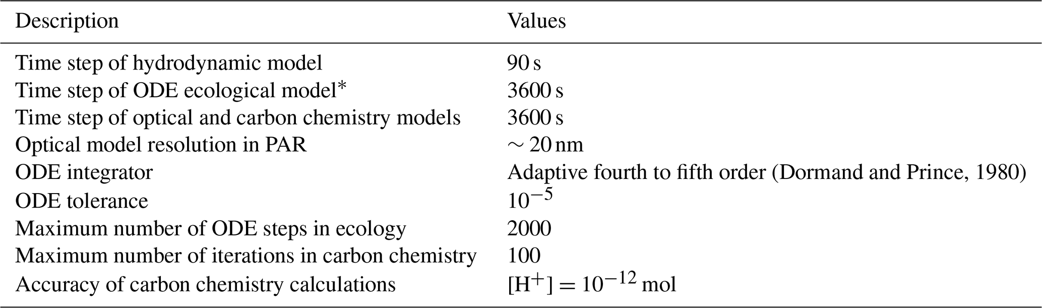
* For the fourth- to fifth-order integrators, the ecological derivatives are evaluated at least every approximately s.
The PDE solvers are described in the physical model description available at https://research.csiro.au/cem/software/ems/ems-documentation/ (last access: 22 September 2020).
The code allows fourth- to fifth-order and seventh- to eighth-order adaptive ODE solvers following Dormand and Prince (1980), as well as the Euler method and adaptive first- and second-order solvers. The preferred scheme is the adaptive fourth–fifth order (similar to ode45 in MATLAB) and implemented in numerous biogeochemical models (Yool, 1997). This requires seven function evaluations for the first step and six for each step after. A relative tolerance of 10−5 is required for each state variable for the integration step to proceed.
The solution of the ecological equations are independent for each vertical column and depend only on the layers above through which the light has propagated. For an nwc-layer water column and nsed-layer sediment, the integrator sequentially solves the top nwc−1 water column layers; the nth water column layer, epibenthic and top sediment layer together; and then the nsed−1 to bottom sediment layers.
10.2 Optical integration
The inherent and apparent optical properties are calculated between the hydrodynamic and ecological integrations. The light field used for each ecological time step is that calculated at the start time of the ecological integration. The spectral resolution of 25 wavebands has been chosen to resolve the absorption peaks associated with Chl a and to span the optical wavelengths. The wavelengths integrated have been chosen such that the lower end of one waveband and the top end of another fall on 400 and 700 nm, respectively, allowing precise calculation of photosynthetically available radiation (PAR).
10.3 Additional integration details
10.3.1 Approximation of stoichiometric coefficients
In this model description, we have chosen to explicitly include atomic mass as integer values, so that the unit conversions are more readable in the equations than if they had all been rendered as mathematical symbols. Nonetheless, these values are more precisely given in the numerical code (Table 41).
Table 41Atomic mass of the C, N, P and O2, both in the model description where two significant figures are used for brevity and in the numerical code, where precision is more important.
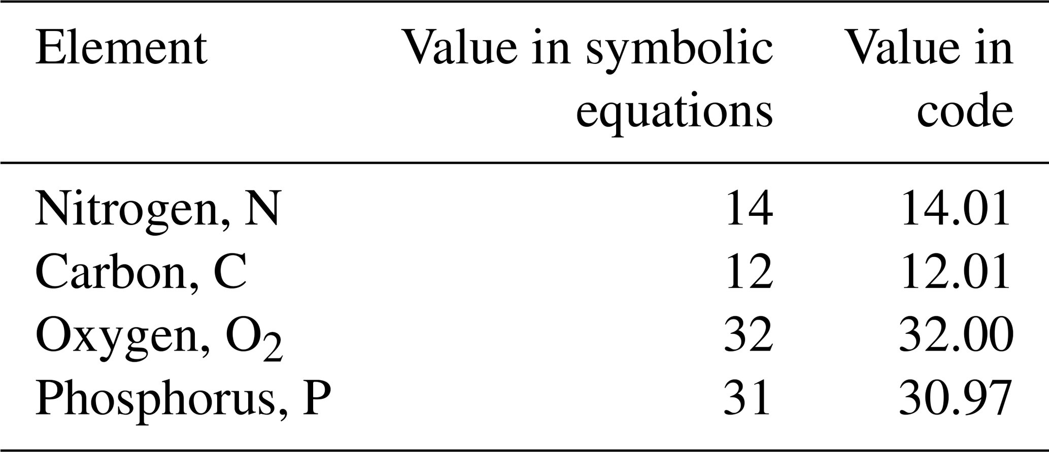
It is worth remembering that the atomic masses are approximations assuming the ratio of isotopes found in the periodic table (Atkins, 1994) based on the natural isotopic abundance of the Earth. So, for example, 14N and 15N have atomic masses of 14.00307 and 15.00011, respectively, with 14N making up 99.64 % of the abundance on Earth. Thus, the value 14.01 comes from . If the model had state variables for 14N and 15N, then the equations would change to contain coefficients of 14 for the 14N isotope equations and 15 for the 15N isotope equations.
10.3.2 Mass conservation in water column and sediment porewaters
A check of mass conservation of total C, TC, total N, TN, total P, TP, and oxygen, [O2], is undertaken in each grid cell at each time step. To establish mass conservation, the sum of the change in mass (of N, P, C and O) with time and the sinks/sources (such as sea–air fluxes, denitrification) must equate to zero.
The total mass and conservation equations are same for the water column and porewaters, with the caveats that (1) air–sea fluxes only affect surface layers of the water, (2) denitrification only occurs in the sediment, and (3) the porosity, ϕ, of the water column is 1. In the sediment, the concentration of particulates is given per unit volume of space, while the concentration of dissolved tracers is given per unit volume of porewater. Thus, the concentration of dissolved tracer, X, per unit space is given by ϕX.
The total carbon in a unit volume of space and its conservation are given by
The total nitrogen in a unit volume of space and its conservation are given by
The total phosphorus in a unit volume of space and its conservation are given by
The concept of oxygen conservation in the model is more subtle than that of C, N and P due to the mass of oxygen in the water molecules not being considered. When photosynthesis occurs, C is transferred from the dissolved phase to reserves within the cell. With both dissolved and particulate pools considered, mass conservation of C is straightforward. In contrast to C, during photosynthesis, oxygen is drawn from the water molecules (i.e. H2O), whose mass is not being considered, and released into the water column. Conversely, when organic matter is broken down, oxygen is consumed from the water column and released as H2O.
In order to obtain a mass conservation for oxygen, the concept of biological oxygen demand (BOD) is used. Often BOD represents the biological demand for oxygen in say a 5 d incubation, BOD5. Here, for the purposes of mass conservation checks, we use BOD∞, the oxygen demand over an infinite time for breakdown. This represents the total oxygen removed from the water molecules for organic matter creation.
Anaerobic respiration reduces BOD∞ without reducing O2 but instead creating reduced-oxygen species. This is accounted for in the oxygen balance by the prognostic tracer COD. In other biogeochemical modelling studies, this is represented by a negative oxygen concentration. Thus, at any time point, the biogeochemical model will conserve the oxygen concentration minus BOD∞ minus COD, plus or minus any sources and sinks such as sea–air fluxes:
where ℛ is respiration of organic matter.
In addition to dissolved oxygen, BOD and COD, nitrate (NO3) appears in the oxygen mass balance. This is necessary because the N associated with nitrate uptake is not taken into the autotrophs but rather released into the water column or porewater. Other entities that contain oxygen in the ocean include the water molecule (H2O) and the phosphorus ion (PO4). In the case of water, this oxygen reservoir is considered very large, with the small flux associated with its change balanced by BOD. In the case of PO4, this is a small reservoir. As oxygen remains bound to P through the entire processes of uptake into reserves and incorporated into structural material and then release, it is not necessary to include it in the oxygen balance for the purposes of ensuring consistency. Nonetheless, strictly the water column and porewater oxygen reservoirs could include a term plus , and the BOD would have similar quantities for reserves and structural material.
10.3.3 Mass conservation in the epibenthic
Mass conservation in the epibenthos requires consideration of fluxes between the water column, porewaters and the epibenthic organisms (macroalgae, seagrass and coral hosts and symbionts). The total carbon in the epibenthos, and its conservation, is given by
where hwc and hsed are the thickness of the bottom water column and top sediment layers, is the normalised internal reserves of carbon in zooxanthellae, 12 g is the rate coral calcification per unit area of coral, Aeff is the area of the bottom covered by coral per m2, and the diffusion terms between porewaters and the water column cancel, so they do not appear in the equations. Note the units of mass of CS needs to be in g N, and some configurations may have multiple seagrass and macroalgae species.
Similarly, for nitrogen, phosphorus and oxygen in the epibenthos,
where there is no dissolved oxygen in the epibenthos.
10.3.4 Unconditional stability
In addition to the above standard numerical techniques, a number of innovations are used to ensure model solutions are reached. Should an integration step fail in a grid cell, no increment of the state variables occurs, and the model continues with a warning flag registered (as Ecology Error). Generally, the problem does not reoccur due to the transport of tracers alleviating the stiff point in phase space of the model. Furthermore, when a water column becomes dry (the sea level drops below the seabed depth), ecological processes are turned off.
The EMS BGC model has been deployed in a range of environments around Australia. With each deployment, a skill assessment has been undertaken (for a history of these applications, see Sect. 13). Recently, the EMS BGC model has been thoroughly assessed against remotely sensed and in situ observations on the GBR as part of the eReefs project (Schiller et al., 2014; Steven et al., 2019b). The assessment of version B1p0 of the eReefs marine model configuration of the EMS included a range of model configurations (4 km, 1 km and relocatable fine-resolution versions) (Herzfeld et al., 2016). The optical and carbon chemistry outputs were assessed in Baird et al. (2016b) and Mongin et al. (2016b), respectively.
A more recent assessment of the BGC model (vB2p0) in the GBR compared simulations against a range of in situ observations that included 24 water quality moorings, two nutrient sampling programmes (with a total of 18 stations) and time series of taxon-specific plankton abundance. In addition to providing a range of skill metrics, the assessment included analysis of seasonal plankton dynamics (Skerratt et al., 2019).
In this section, we assess version B3p0 in the 4 km GBR configuration. First, we consider the behaviour of the microalgae physiology as a means to understanding the dynamics of the microalgal growth model. Secondly, the techniques and observations used in Skerratt et al. (2019) have been applied to the model version described in this paper (vB3p0) with highlights discussed here and the full analysis appearing in the Supplement.
11.1 Analysis of microalgae growth and pigment synthesis dynamics
The microalgae growth model (Sect. 5.1.1) was derived from first quantifying the fluxes into a cell of energy (for fixing carbon), N, P and O. Each flux adds to the reserves of that element in the cell. A second process, the consumption of reserves to create microalgae structural material with a constant stoichiometry (), increases the number of cells but reduces the reserves of each element both per cell and of the population. Thus, the microalgae in the growth model are generating organic matter at the Redfield ratio while being exposed to external nutrient fields at non-Redfield ratios. At the same time as the microalgae grow, the model represents the synthesis of chlorophyll based on the cell's need for more carbon fixation and the benefit of adding pigment on the rate of photon absorption (Fig. 11).
To illustrate these dynamics, we look at a vertical profile of a deep site in the Coral Sea with a 1 and 2.5 µm radius microalgae (Fig. 13). The expectation is that, for the same environmental conditions, the 1 µm cell will be less nutrient limited and more light limited than the 2.5 µm cell – a result of the 1 µm cell having a greater diffusion rate per unit volume than the larger cell. Further, that near-surface cells will be more nutrient limited, deeper cells more light limited. Finally, light-limited cells will generally have more pigment per cell.
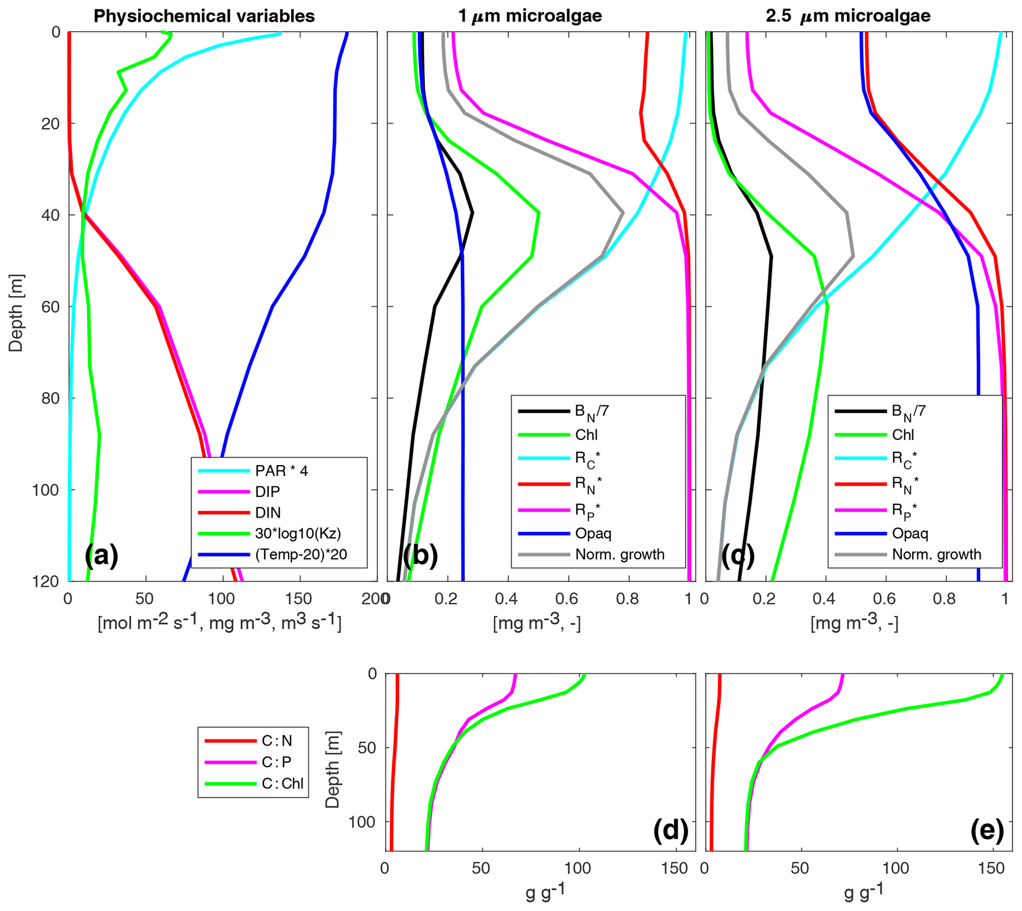
Figure 13Vertical profiles of physiochemical variables (a) and physiological variables from 1 µm (b, d) and 2.5 µm (c, e) radii microalgae. Panel (a) shows photosynthetically available radiation (PAR; mol m−2 s−1), dissolved inorganic phosphorus (DIP; mg P m−3), dissolved inorganic nitrogen (DIN; mg N m−3), vertical diffusivity (Kz; m3 s−1) and temperature (∘C). Panels (b) (1 µm) and (c) (2.5 µm) show biomass of structural material in nitrogen (BN; mg N m−3), chlorophyll a concentration (Chl; mg Chl a m−3), normalised reserves of fixed carbon (), nitrogen () and phosphorus (), cell opaqueness (absorption cross-section divided by projected area, α∕(πr2)) and normalised growth rate of . Panels (d) (1 µm) and (e) (2.5 µm) show stoichiometric ratios of carbon to nitrogen (C:N), phosphorus (C:P) and chlorophyll (C:Chl a). PAR, Kz, temperature and BN are all scaled for plotting.
In addition to being a measure of the quantity of nutrient reserves, normalised reserves (R*) of each nutrient is a metric of how limiting that nutrient is, with 1 being unlimited, and 0 being completely limited. At the surface at midday, the 1 µm cells have a biomass of 0.2 mg m−3 (Fig. 13b). The cells are strongly phosphorus limited (), slightly nitrogen limited ( = 0.86) and almost light unlimited (). The realised growth rate, as a fraction of the maximum growth rate, is . The larger cells are more nutrient limited (, ), and again light unlimited (), realising a normalised growth rate of 0.07 (Fig. 13c).
The elemental ratios of the microalgae can be calculated from the reserves (in wt wt−1: ; ). The C:N and C:P ratios are both higher in the nutrient-replete surface waters, with C:P varying more due to greater P limitation in the surface waters. A deep chlorophyll maximum has formed for the 1 µm microalgae at 40 m and for 2.5 µm microalgae at 60 m. Here, we will explain this distribution based on microalgae growth alone (ignoring grazing and sinking terms). The 1 µm microalgae has a growth maximum at 40 m, as nutrients have become non-limiting and fixed carbon reserves are still relatively high (). Growth below 50 m becomes primarily light limited, so normalised growth is equal to normalised fixed carbon reserves. The 2.5 µm microalgae are nutrient limited deeper into the water column, resulting in a deep growth maximum.
The 1 and 2.5 µm cells have a slight biomass maximum at 40 and 50 m, respectively, but the chlorophyll maximum is more pronounced (Fig. 13b, c). At the surface, the 1 µm microalgae have low pigment content and are therefore relatively transparent (opaqueness, or the absorption cross-section divided by the projected area, α∕(πr2), is 0.11), with a C:Chl ratio of 100 [g g−1]. At the deep chlorophyll maxima for 1 µm cells, the pigment content has increased, as shown by the C:Chl dropping to 20 [g g−1], the minimum C:Chl ratio observed in the ocean (Sathyendranath et al., 2009), resulting in an opaqueness of 0.25. The 2.5 µm cells are less light limited than the smaller cells. At the surface, chlorophyll synthesis generates in 2.5 µm cells an opaqueness of 0.52. Given the larger size of the cell, this is achieved at a C:Chl ratio of 150. At the 50 m deep chlorophyll maxima, the C:Chl dropped to 20, but in the larger cells this achieves an opaqueness of 0.91 (i.e. the absorption cross-section is almost equal to the projected area).
In summary, the application of simple physical limits to uptake, a restraint of constant stoichiometric conversion to structural material, and cells synthesising chlorophyll to maximise photon absorption when light limited, generates the typical physiological properties of microalgae seen in vertical profiles in the ocean.
11.2 Model assessment of the GBR configuration
A detailed comparison of a GBR simulation against observations of Chl a concentration, dissolved inorganic carbon, nitrogen, phosphorus and ammonium, dissolved organic nitrogen and phosphorus, alkalinity, pH, aragonite saturation, mass of suspended sediments, turbidity and Secchi depth appears in the Supplement. Here, we highlight the carbon chemistry, nutrient and plankton components that are driven by the BGC model.
11.2.1 Chlorophyll dynamics
The most accurate measurements of water column chlorophyll concentrations in the GBR are obtained using high-performance liquid chromatography (HPLC) and chlorophyll extractions from water column samples. Chlorophyll extractions have been taken at 36 locations along the GBR (S5, Sect. 10; for site locations, see S5, Sect. E1). As an example, a time series at Pelorus Island in the central GBR (Fig. 14) shows large variability in both the observations and the simulations, driven by interannual climatic forcing, with 2011–2013 experiencing much greater river loads than 2014–2016, intra-annual trends driven by greater loads of nutrients during the wet season (January–June) than the remainder of the year, as well as monthly variability related to tidal movements and predator–prey oscillations. Even given this variability, comparison of the instantaneous state of the simulations against extracted chlorophyll concentrations showed the model was able to achieve across all 36 sites a bias ± root mean square error (RMSE) of mg m−3 (Fig. 15).
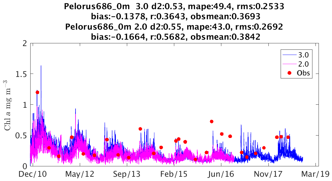
Figure 14Observed surface chlorophyll concentration from chlorophyll extraction (red dots) at the Pelorus Island Marine Monitoring Program site ( S, E) with a comparison to configurations vB2p0 (pink line) and vB3p0 (blue line). Statistics listed include the Willmott d2 metric (Willmott et al., 1985), mean absolute percent error (MAPE) and RMSE.
Moored fluorometers are generally less accurate than chlorophyll extractions but provide a greater temporal resolution of chlorophyll dynamics. Here, we show observations from a mooring at Palm Passage (Fig. 16), away from the influence of the river discharge and dependent primary on shelf break interactions. The observed time series from 60 m depth show interannual variability in fluorescence related to primarily to an October–March maximum in intrusion events (for details of deployment details and oceanographic processes, see Benthuysen et al., 2016), which are also seen in the vB3p0 simulations. Comparison to other moored fluorometers on the GBR (S5, Sects. 19 and 21) shows a range of predictive skill.
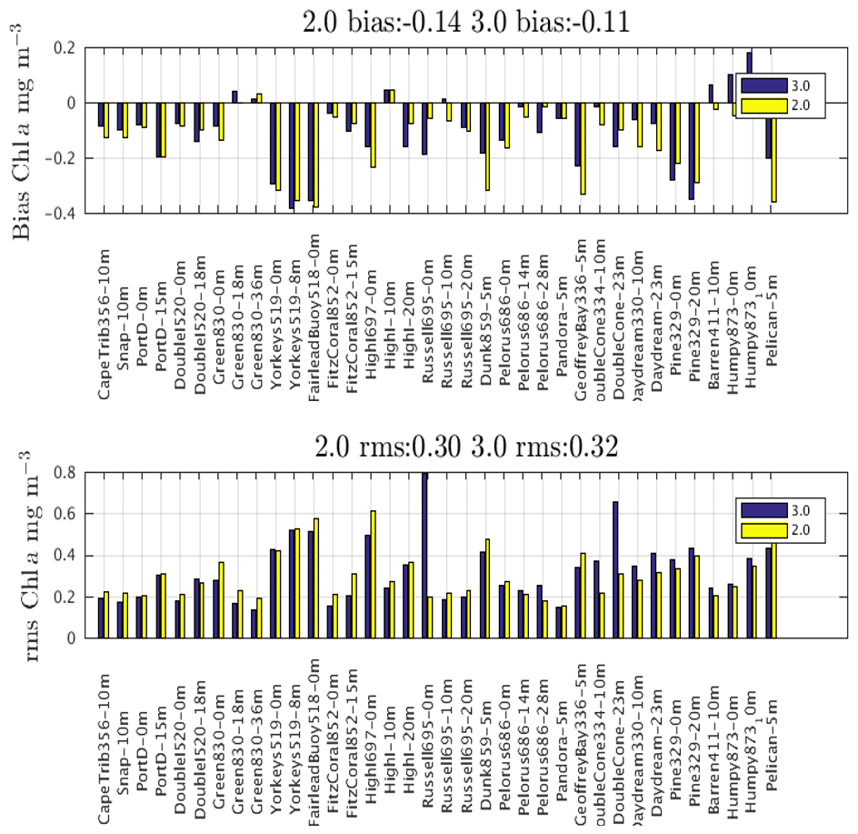
11.2.2 Nutrient dynamics
The model represents dissolved nitrate, ammonium and phosphorus nutrients. In the surface waters of the inshore GBR, nutrients are generally at very low concentrations, with modest increases seen each wet season. At High Island in the central GBR (Fig. 17), DIP has a mean concentration of 2 mg m−3, with concentrations varying between 0 and 5 mg m−3. The concentrations of nitrate and ammonium are both very low, with occasional peaks driven by river plume exposure. The simulated nutrients generally follow the expected time-varying patterns: peaks in the wet season, larger peaks in the wettest years (2011, 2012, 2013, 2018) and extremely low concentrations in the dry seasons. Across all sites (S5, Sect. 13), vB3p0 predicted DIP with a skill of (bias ± RMSE) of mg P m−3, nitrate of mg N m−3 and ammonium of mg N m−3.
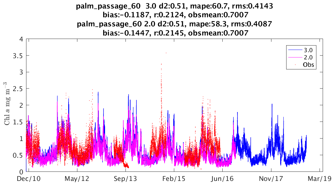
Figure 16Observed chlorophyll fluorescence (red dots) at 60 m depth at the Palm Passage site with a comparison to configurations vB3p0 (blue) and vB2p0 (pink).

Figure 17Dissolved inorganic phosphorus (a), nitrate (b) and ammonium (c) concentrations at High Island, central GBR: observations (red dots), simulations vB2p0 (pink) and vB3p0 (blue).
11.2.3 Carbon chemistry
The model contains two state variables to represent the state of carbon chemistry, dissolved inorganic carbon and alkalinity, from which, at equilibrium and known temperature and salinity, other variables such as pH may be calculated. The biogeochemical model provides highly skilful predictions of pH and aragonite saturation (Fig. 18). This success is primarily due to the skill of the hydrodynamic model. The circulation produces a good representation of the alkalinity field, and the sea surface temperature sets an accurate difference in the partial pressure of CO2 between the atmosphere and ocean. With these phenomena accurately calculated, the model needs only to correctly predict the time-averaged wind-speed-dependent air–sea flux. Further assessment of carbon chemistry properties along the entire length of the GBR (S5; Sect. 28) shows a bias ± RMSE of DIC of mmol m−3. Further skill assessment from inshore sites is available in Mongin et al. (2016b).
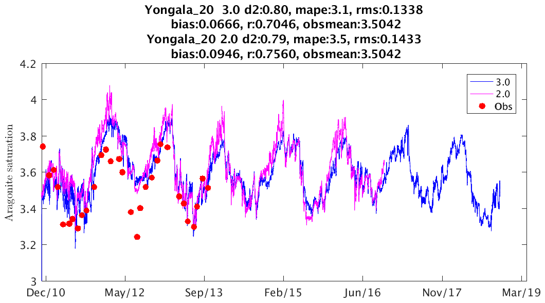
Figure 18Aragonite saturation state calculated from temperature, DIC and alkalinity at 20 m depth at the Integrated Marine Observing System (IMOS) Yongala mooring, central GBR: observations (red dots), simulations B2p0 (pink) and B3p0 (blue).
The outputs of all hindcasts in the eReefs project can be downloaded from http://dapds00.nci.org.au/thredds/catalogs/fx3/catalog.html (last access: 22 September 2020).
A web-based interface, RECOM, has been developed to automate the process of downscaling the EMS model using an existing hindcast as boundary conditions (https://research.csiro.au/ereefs/models/models-about/recom/, last access: 22 September 2020, including the RECOM User Manual). For the purposes of learning how to apply the EMS software available, RECOM provides the user with the ability to generate a complete test case of a domain situated along the northeast Australian coastline. Once a RECOM simulation has been generated using the web interface, the entire simulation including source code, forcing and initial condition files, model configuration files and the model output can be downloaded. This allows the user to repeat the model simulation on their own computing system and modify code, forcing and output frequency as required. The technical details of RECOM are detailed in Baird et al. (2018) and in the RECOM user manual.
The EMS BGC model development has been a function of the historical applications of the model across a rage of ecosystems, so it is worth giving a brief history of the model development.
13.1 History of the development of the EMS biogeochemical model
The EMS biogeochemical model was first developed as a nitrogen-based model for determining the assimilative capacity for sewerage discharged into Port Philip Bay, the embayment of the city of Melbourne (Harris et al., 1996). This study saw a focus on sediment processes such as denitrification and demonstrated the ability of bay-wide denitrification to prevent change in the ecological state of the bay exposed to sewerage treatment plant loads (Murray and Parslow, 1997; Murray and Parlsow, 1999). The basic structure of the model and in particular the split of pelagic, epibenthic and sediment zones were in place for this project. This zonation generated the ability to resolve processes in shallow-water systems and in particular to consider benthic flora in detail.
The next major study involved simulating a range of estuarine morphologies (salt wedge, tidal, lagoon, residence times) and forcings (river flow seasonality, nutrient inputs, etc.) that were representative of Australia's 1000+ estuaries (Baird et al., 2003). At this point, carbon and phosphorus were included in the model, and the process of including physical limits to ecological processes begun (e.g. diffusion limitation of nutrient uptake and encounter-rate limitation of grazing).
Following studies in the phosphorus-limited Gippsland Lakes and macro-tidal Ord River system led to the refinement of the phosphorus absorption–desorption processes. Further studies of the biogeochemical–sediment interactions in the subtropical Fitzroy River (Robson et al., 2006) and investigation of the impacts of a tropical cyclone (Condie et al., 2009), saw a stronger link to remote observations. At this time, the use of offline transport schemes were also implemented (such as the Moreton Bay model), allowing for an order-of-magnitude faster model integration (Gillibrand and Herzfeld, 2016).
The next major change in the BGC model involved implementing variable ratios of microalgae through the introduction of reserves of energy, nitrogen and phosphorus (Wild-Allen et al., 2010), allowing for more accurate prediction of the elemental budgets and impacts of natural and anthropogenic forcing of the Derwent River estuary, southeast Tasmania. This study was followed up by a number of studies developing scenarios to inform management strategies of the region (Wild-Allen et al., 2011, 2013; Skerratt et al., 2013; Hadley et al., 2015a, b).
From 2010 onwards, EMS has been applied to consider the impacts of catchment loads on the Great Barrier Reef. The focus on water clarity led to the development of a spectrally resolved optical model and the introduction of simulated true colour (Baird et al., 2016b). The eReefs project was the first EMS application to consider corals with the introduction of the host–symbiont coral system and equilibrium carbon chemistry (Mongin and Baird, 2014; Mongin et al., 2016b, a). Additionally, the calculation of model outputs that match remote-sensing observations allowed the model to be run in a data-assimilating system, where the observation–model mismatch was based on remote-sensing reflectance (Jones et al., 2016). The most recent application of the EMS BGC model has been for investigating the environmental impact of aquaculture in Los Lagos, Chile (Steven et al., 2019a). For the Los Lagos application, new processes for fish farms, dinoflagellates and benthic filter feeders were added, although these additions are not described in this document. As a demonstration of the ability to add and remove processes, the Los Lagos application was run with the same EMS C-executable file as the Great Barrier Reef application, just with the configuration files altered.
13.2 Comparison with other marine biogeochemical models
As introduced earlier, there are a number of complex marine biogeochemical models. The most similar model in scope and approach to EMS is the ERSEM (European Regional Seas Ecosystem Model) model (Butenschön et al., 2016). Both ERSEM and EMS consider in detail pelagic, benthic and sediment processes and could generally be described as functional group models. That is, the state variables and the processes that link them are chosen to represent groups of organisms that act in similar ways. This allows the complexity of real systems to be reduced to a tractable model. Many functional group style biogeochemical models exist and were in fact the earliest models developed (Riley, 1947; Fasham, 1993; Sarmiento et al., 1993). The most significant differences between EMS and ERSEM are (1) EMS concentrates more on benthic flora than ERSEM, while ERSEM considers lower-trophic-level ecosystem interactions such as fisheries that are not captured in EMS; and (2) while EMS and ERSEM have similar state variables and processes, EMS has a different set of governing equations that are based on geometric constraints of individuals while ERSEM, like most other functional biogeochemical models, has equations based on empirical relationships determined from population interactions.
The last two decades have seen addition modelling approaches emerge: trait-based models that consider changing processes rates as populations vary (Bruggeman and Kooijman, 2007); size-based models that determine rates based on organism size (Baird et al., 2007a); ecosystem-style models that consider a multiple “species” within a functional group, developing large food webs (Fulton et al., 2014); and models that consider a large number of functional groups that are refined through competition between groups (Follows et al., 2007). These new approaches are applied primarily in pelagic ecosystems, where the generic nature of pelagic interactions encourages overarching philosophies to model construction and with considerable success (Dutkiewicz et al., 2015). The awkwardness of the variety of benthic communities (corals, seagrass, kelp, etc.) and their prime role in shallow water, has meant that estuarine and coastal models have, like ERSEM and EMS, typically chosen the functional model approach (Madden and Kemp, 1996; Spillman et al., 2007).
13.3 Future developments in EMS
EMS has been developed to address specific scientific questions in Australia's coastal environment. As a result, the set of processes the EMS considers varies from those typically applied by other groups developing marine BGC models. Processes which have not been considered but often are considered in marine BGC models, include iron and silicate limitation (which are not common on the Australian continental shelf or estuaries), photo-inhibition of microalgae, explicit bacterial biomass. Each of these will be considered as the need arises.
A deliberate decision in the development of the EMS BGC model was made to avoid higher-trophic-level processes, such fish dynamics and reproduction of long-lived species. This decision was made because (1) including these longer timescale, often highly non-linear, processes reduces the ability of development to concentrate on BGC processes; and (2) it was recognised that CSIRO has developed a widely used ecosystem model (Atlantis, https://research.csiro.au/atlantis/, last access: 22 September 2020; Fulton et al., 2014), and that coupling the EMS with Atlantis takes advantage of complementary strengths of the two modelling systems.
A recent capacity introduced to EMS is the development of a relocatable capability (RECOM; Sect. 12), allowing model configurations (grid, river and meteorological forcing, ecological processes, boundary conditions) to be automatically generated. This capability will be a good test of the portability of the BGC model and in particular the use of geometric description of physical limits to ecological processes.
Future enhancements in the EMS BGC model for tropical systems are likely to continue to pursue those components at risk from human impacts, such as dissolution of marine carbonates affecting sediment substrate and herbicide interactions with photosystems. We also expect to continue to refine the optical model and in particular the relationship between particle size distribution and mass-specific scattering and absorption properties. In temperate systems, current and near-future deployments of EMS in Australia will be focused on coastal system characterisation for aquaculture, carbon sequestration and management decision support for the blue economy. Ongoing research includes improved methods for model validation against observations and translation of model outputs into knowledge that informs stakeholder decisions.
13.4 Concluding thoughts
The BGC model in the CSIRO EMS has developed unique parameterisation when compared to other marine biogeochemical models applied elsewhere due in part to a unique set of scientific challenges of the Australian coastline. It has proved to be useful in many applications, most notably the Great Barrier Reef where extensive observational datasets has allowed new process model development and detailed model skill assessment (Baird et al., 2016b, a; Mongin et al., 2016b; Skerratt et al., 2019 and http://ereefs.info/, last access: 22 September 2020). This document provides easy access to some of the novel process formulations that have been important in this success, as well as a complete scientific description of version B3p0.
The model web page is https://research.csiro.au/cem/software/ems/ (last access: 22 September 2020).
The web page links to an extensive user guide for the entire EMS package, which contains any information that is generic across the hydrodynamic, sediment, transport and ecological models, such as input/output formats. A smaller biogeochemical user guide documents details relevant only to the biogeochemical and optical models (such as how to specify wavelengths for the optical model), and a biogeochemical developer's guide describes how to add additional processes to the code.
A permanent link to the EMS C code used in this paper is (CSIRO, 2019) https://doi.org/10.25919/5e701c5c2d9c9.
The code available is also available on GitHub at https://github.com/csiro-coasts/EMS/ (CSIRO, 2020a), which continues to be developed. The version is labelled as vB3p0 to distinguish it from earlier versions of the ecological library used in the eReefs project and others. On the GitHub site, vB3p0 is referred to as ecology v1.1.1, is contained within EMS release v1.1 in the GitHub archive and can be accessed at https://github.com/csiro-coasts/EMS/releases/tag/v1.1.1 (CSIRO, 2020b).
The list of processes that this paper describes is given in a configuration file in the Supplement (S1). The library contains other processes that have been retained for backward comparability or for other applications (i.e. mussel farms). The methods by which differential equations described in this scientific description are incorporated into the model code are described in the Supplement (S2).
The supplement related to this article is available online at: https://doi.org/10.5194/gmd-13-4503-2020-supplement.
All authors contributed to the CSIRO EMS BGC model through either proposing model formulations, writing significant components of the code or applying the model. The primary model developers were MEB, KWA, JP, MM, BR and FR. MEB wrote the manuscript with co-authors contributing analyses, figures and revisions. JS and MEB prepared the article Supplements.
The authors declare that they have no conflict of interest.
Many scientists and projects have contributed resources and knowhow to the development of this model over 20+ years. For this dedication, we are very grateful. Those who have contributed to the numerical code (CSIRO unless stated) include
Mike Herzfeld, Philip Gillibrand, John Andrewartha, Farhan Rizwi, Jenny Skerratt, Mathieu Mongin, Mark Baird, Karen Wild-Allen, John Parlsow, Emlyn Jones, Nugzar Margvelashvili, Pavel Sakov (BOM, who introduced the process structure), Jason Waring, Stephen Walker, Uwe Rosebrock, Brett Wallace, Ian Webster, Barbara Robson (AIMS), Scott Hadley (University of Tasmania), Malin Gustafsson (University of Technology Sydney, UTS) and Matthew Adams (Queensland University of Technology).
We also thank Britta Schaffelke and her colleagues in the Marine Monitoring Program for their commitment to obtaining the observations that enabled the model evaluation. We also acknowledge the use of data from the AIMS Long Term Monitoring Program, Australia's Integrated Marine Observing System and the Future Reef 2.0 Program funded by GBRF, Rio Tinto and CSIRO. We greatly appreciate Cedric Robillot for his leadership of the eReefs project.
Collaborating scientists include Andy Steven, Thomas Schroeder, Bronte Tilbrook, Craig Neill, John Akl, Erik van Ooijen, Nagur Cherukuru, Peter Ralph (UTS), Russ Babcock, Kadija Oubelkheir, Bojana Manojlovic (UTS), Stephen Woodcock (UTS), Stuart Phinn (UQ), Chris Roelfsema (UQ), Miles Furnas (AIMS), David McKinnon (AIMS), David Blondeau-Patissier (Charles Darwin University), Michelle Devlin (James Cook University), Eduardo da Silva (JCU), Julie Duchalais, Jerome Brebion, Leonie Geoffroy, Yair Suari, Cloe Viavant, Lesley Clementson (pigment absorption coefficients), Dariusz Stramski (inorganic absorption and scattering coefficients), Erin Kenna, Line Bay (AIMS), Neal Cantin (AIMS), Luke Morris (AIMS), Daniel Harrison (SCU) and Karlie MacDonald.
Funding bodies include CSIRO Wealth from Oceans Flagship, Gas Industry Social & Environmental Research Alliance (GISERA), CSIRO Coastal Carbon Cluster, Derwent Estuary Program, INFORM2, eReefs, Great Barrier Reef Foundation, Australian Climate Change Science Program, University of Technology Sydney, Department of Energy and Environment, Integrated Marine Observing System (IMOS), National Environment Science Program (NESP TWQ Hub) and the Royal Australian Navy.
Finally, we greatly appreciate Marcello Vichi's in-depth and insightful review that has much improved the manuscript.
This paper was edited by Julia Hargreaves and reviewed by Marcello Vichi and one anonymous referee.
Anthony, K. R. N., Kleypas, J. A., and Gattuso, J.-P.: Coral reefs modify their seawater carbon chemistry - implications for impacts of ocean acidification, Glob. Change Biol., 17, 3655–3666, 2011. a
Atkins, P. W.: Physical Chemistry, Oxford University Press, Oxford, 5th Edn., 1994. a
Atkinson, M. J.: Productivity of Eniwetak Atoll reef predicted from mass-transfer relationships, Cont. Shelf Res., 12, 799–807, 1992. a
Atkinson, M. J. and Bilger, B. W.: Effects of water velocity on phosphate uptake in coral reef-flat communities, Limnol. Oceanogr., 37, 273–279, 1992. a
Atkinson, M. J. and Smith, S. V.: C:N:P ratios of benthic marine plants, Limnol. Oceanogr., 28, 568–574, 1983. a
Aumont, O., Ethé, C., Tagliabue, A., Bopp, L., and Gehlen, M.: PISCES-v2: an ocean biogeochemical model for carbon and ecosystem studies, Geosci. Model Dev., 8, 2465–2513, https://doi.org/10.5194/gmd-8-2465-2015, 2015. a
Babcock, R. C., Baird, M. E., Pillans, R., Patterson, T., Clementson, L. A., Haywood, M. E., Rochester, W., Morello, E., Kelly, N., Oubelkheir, K., Fry, G., Dunbabin, M., Perkins, S., Forcey, K., Cooper, S., Donovan, A., Kenyon, R., Carlin, G., and Limpus, C.: Towards an integrated study of the Gladstone marine system, 278 pp., ISBN: 978-1-4863-0539-1, Tech. rep., CSIRO Oceans and Atmosphere Flagship, Brisbane, 2015. a
Baird, M. E.: Numerical approximations of the mean absorption cross-section of a variety of randomly oriented microalgal shapes, J. Math. Biol., 47, 325–336, 2003. a
Baird, M. E. and Emsley, S. M.: Towards a mechanistic model of plankton population dynamics, J. Plankton Res., 21, 85–126, 1999. a
Baird, M. E. and Middleton, J. H.: On relating physical limits to the carbon: nitrogen ratio of unicellular algae and benthic plants, J. Marine Sys., 49, 169–175, 2004. a, b
Baird, M. E., Emsley, S. M., and McGlade, J. M.: Modelling the interacting effects of nutrient uptake, light capture and temperature on phytoplankton growth, J. Plankton Res., 23, 829–840, 2001. a, b
Baird, M. E., Walker, S. J., Wallace, B. B., Webster, I. T., and Parslow, J. S.: The use of mechanistic descriptions of algal growth and zooplankton grazing in an estuarine eutrophication model, Estuar. Coast. Shelf Sci., 56, 685–695, 2003. a, b, c, d, e
Baird, M. E., Oke, P. R., Suthers, I. M., and Middleton, J. H.: A plankton population model with bio-mechanical descriptions of biological processes in an idealised 2-D ocean basin, J. Marine Sys., 50, 199–222, 2004. a, b, c, d, e
Baird, M. E., Timko, P. G., Suthers, I. M., and Middleton, J. H.: Coupled physical-biological modelling study of the East Australian Current with idealised wind forcing: Part II: Biological dynamical analysis, J. Marine Sys., 59, 271–291, 2006. a
Baird, M. E., Leth, O., and Middleton, J. F.: Biological response to circulation driven by mean summertime winds off central Chile: A numerical model study, J. Geophys. Res., 112, C07031, https://doi.org/10.1029/2006JC003655, 2007a. a
Baird, M. E., Timko, P. G., and Wu, L.: The effect of packaging of chlorophyll within phytoplankton and light scattering in a coupled physical-biological ocean model., Mar. Fresh. Res., 58, 966–981, 2007b. a
Baird, M. E., Ralph, P. J., Rizwi, F., Wild-Allen, K. A., and Steven, A. D. L.: A dynamic model of the cellular carbon to chlorophyll ratio applied to a batch culture and a continental shelf ecosystem, Limnol. Oceanogr., 58, 1215–1226, 2013. a, b, c, d
Baird, M. E., Adams, M. P., Babcock, R. C., Oubelkheir, K., Mongin, M., Wild-Allen, K. A., Skerratt, J., Robson, B. J., Petrou, K., Ralph, P. J., O'Brien, K. R., Carter, A. B., Jarvis, J. C., and Rasheed, M. A.: A biophysical representation of seagrass growth for application in a complex shallow-water biogeochemical model, Ecol. Model., 325, 13–27, 2016a. a, b, c, d, e, f, g, h, i, j
Baird, M. E., Cherukuru, N., Jones, E., Margvelashvili, N., Mongin, M., Oubelkheir, K., Ralph, P. J., Rizwi, F., Robson, B. J., Schroeder, T., Skerratt, J., Steven, A. D. L., and Wild-Allen, K. A.: Remote-sensing reflectance and true colour produced by a coupled hydrodynamic, optical, sediment, biogeochemical model of the Great Barrier Reef, Australia: comparison with satellite data, Environ. Modell. Softw., 78, 79–96, 2016b. a, b, c, d, e, f
Baird, M. E., Mongin, M., Rizwi, F., Bay, L. K., Cantin, N. E., Soja-Woźniak, M., and Skerratt, J.: A mechanistic model of coral bleaching due to temperature-mediated light-driven reactive oxygen build-up in zooxanthellae, Ecol. Model., 386, 20–37, 2018. a, b, c, d
Baretta-Bekker, J., Baretta, J., and Ebenhöh, W.: Microbial dynamics in the marine ecosystem model ERSEM II with decoupled carbon assimilation and nutrient uptake, J. Sea Res., 38, 195–211, 1997. a
Beckmann, A. and Hense, I.: Torn between extremes: the ups and downs of phytoplankton, Ocean Dynam., 54, 581–592, 2004. a
Benthuysen, J. A., Tonin, H., Brinkman, R., Herzfeld, M., and Steinberg, C.: Intrusive upwelling in the Central Great Barrier Reef, J. Geophys. Res.-Oceans, 121, 8395–8416, 2016. a
Blondeau-Patissier, D., Brando, V. E., Oubelkheir, K., Dekker, A. G., Clementson, L. A., and Daniel, P.: Bio-optical variability of the absorption and scattering properties of the Queensland inshore and reef waters, Australia, J. Geophys. Res.-Oceans, 114, C05003, https://doi.org/10.1029/2008JC005039, 2009. a, b, c
Bohren, C. F. and Huffman, D. R.: Absorption and scattering of light particles by small particles, John Wiley & Sons, 1983. a
Boudreau, B. P.: A method-of-lines code for carbon and nutrient diagenesis in aquatic sediments, Comput. Geosci., 22, 479–496, 1996. a
Bruggeman, J. and Kooijman, S. A. L. M.: A biodiversity-inspired approach to aquatic ecosystem modeling, Limnol. Oceanogr., 52, 1533–1544, 2007. a
Butenschön, M., Zavatarelli, M., and Vichi, M.: Sensitivity of a marine coupled physical biogeochemical model to time resolution, integration scheme and time splitting method, Ocean Model., 52–53, 36–53, 2012. a, b
Butenschön, M., Clark, J., Aldridge, J. N., Allen, J. I., Artioli, Y., Blackford, J., Bruggeman, J., Cazenave, P., Ciavatta, S., Kay, S., Lessin, G., van Leeuwen, S., van der Molen, J., de Mora, L., Polimene, L., Sailley, S., Stephens, N., and Torres, R.: ERSEM 15.06: a generic model for marine biogeochemistry and the ecosystem dynamics of the lower trophic levels, Geosci. Model Dev., 9, 1293–1339, https://doi.org/10.5194/gmd-9-1293-2016, 2016. a, b, c
Cambridge, M. L. and Lambers, H.: Specific leaf area and functional leaf anatomy in Western Australian seagrasses, in: Inherent variations in plant growth: physiological mechanisms and ecological consequences, edited by: Lambers, H., Poorter, H., and Vuren, M. M. I. V., Backhuys, Leiden, 88–99, 1998. a
Carpenter, E., O’Neil, J., Dawson, R., Capone, D., Siddiqui, P., Roenneberg, T., and Bergman, B.: The tropical diazotrophic phytoplankter Trichodesmium: Biological characteristics of two common species, Mar. Ecol. Prog. Ser., 95, 295–304, 1993. a
Chartrand, K. M., Ralph, P. J., Petrou, K., and Rasheed, M. A.: Development of a Light-Based Seagrass Management Approach for the Gladstone Western Basin Dredging Program, Tech. rep., DAFF Publication. Fisheries Queensland, Cairns 126 pp., 2012. a
Chartrand, K. M., , Bryant, C. V., Sozou, A., Ralph, P. J., and Rasheed, M. A.: Final Report: Deepwater seagrass dynamics: Light requirements, seasonal change and mechanisms of recruitment, Tech. rep., Centre for Tropical Water and Aquatic Ecosystem Research (TropWATER) Publication, James Cook University, Report No 17/16, Cairns, 67 pp., 2017. a
Cherukuru, N., Dekker, A. G., Hardman-Mountford, N. J., Clementson, L. A., and Thompson, P. A.: Bio-optical variability in multiple water masses across a tropical shelf: Implications for ocean colour remote sensing models, Estuar. Coast. Shelf Sci., 219, 223–230, 2019. a
Clementson, L. A. and Wojtasiewicz, B.: Dataset on the absorption characteristics of extracted phytoplankton pigments, Data in Brief, 24, 103875, https://doi.org/10.1016/j.dib.2019.103875, 2019. a, b
Condie, S. A., Herzfeld, M., Margvelashvili, N., and Andrewartha, J. R.: Modeling the physical and biogeochemical response of a marine shelf system to a tropical cyclone, Geophys. Res. Lett., 36, L22603, https://doi.org/10.1029/2009GL039563, 2009. a, b
CSIRO: EMS Release v1.1.1. v1. CSIRO, Software Collection, https://doi.org/10.25919/5e701c5c2d9c9, 2019. a
CSIRO Coastal Environmental Modelling Team: CSIRO Environmental Modelling Suite GitHub archive, available at: https://github.com/csiro-coasts/EMS/, last access: 22 September 2020a. a
CSIRO Coastal Environmental Modelling Team: CSIRO Environmental Modelling Suite GitHub archive v1.1.1, available at: https://github.com/csiro-coasts/EMS/releases/tag/v1.1.1, last access: 22 September 2020. a
Dietze, H., Matear, R., and Moore, T.: Nutrient supply to anticyclonic meso-scale eddies off western Australia estimated with artificial tracers released in a circulation model, Deep-Sea Res. Pt. I, 56, 1440–1448, 2009. a
Dormand, J. R. and Prince, P. J.: A family of embedded Runge-Kutta formulae, J. Comp. Appl. Math., 6, 19–26, 1980. a, b
Duarte, C. M. and Chiscano, C. L.: Seagrass biomass and production: a reassessment, Aquat. Bot., 65, 159–174, 1999. a
Dutkiewicz, S., Hickman, A. E., Jahn, O., Gregg, W. W., Mouw, C. B., and Follows, M. J.: Capturing optically important constituents and properties in a marine biogeochemical and ecosystem model, Biogeosciences, 12, 4447–4481, https://doi.org/10.5194/bg-12-4447-2015, 2015. a, b, c
Duysens, L. N. M.: The flattening of the absorption spectra of suspensions as compared to that of solutions, Biochim. Biophys. Acta, 19, 1–12, 1956. a, b, c
Eyre, B. D., Cyronak, T., Drupp, P., Carlo, E. H. D., Sachs, J. P., and Andersson, A. J.: Coral reefs will transition to net dissolving before end of century, Science, 359, 908–911, 2018. a, b
Falter, J. L., Atkinson, M. J., and Merrifield, M. A.: Mass-transfer limitation of nutrient uptake by a wave-dominated reef flat community, Limnol. Oceanogr., 49, 1820–1831, 2004. a
Fasham, M. J. R.: Modelling the marine biota, in: The Global Carbon Cycle, edited by: Heimann, M., Springer-Verlag, New York, 457–504, 1993. a, b
Fasham, M. J. R., Ducklow, H. W., and McKelvie, S. M.: A nitrogen-based model of plankton dynamics in the oceanic mixed layer, J. Mar. Res., 48, 591–639, 1990. a
Fennel, K., Gehlen, M., Brasseur, P., Brown, C. W., Ciavatta, S., Cossarini, G., Crise, A., Edwards, C. A., Ford, D., Friedrichs, M. A. M., Gregoire, M., Jones, E. M., Kim, H.-C., Lamouroux, J., Murtugudde, R., and Perruche, C.: Advancing marine biogeochemical and ecosystem reanalyses and forecasts as tools for monitoring and managing ecosystem health, Front. Mar. Sci., 6, 89, https://doi.org/10.3389/fmars.2019.00089, 2019. a
Ficek, D., Kaczmarek, S., Stoń-Egiert, J., Woźniak, B., Majchrowski, R., and Dera, J.: Spectra of light absorption by phytoplankton pigments in the Baltic; conclusions to be drawn from a Gaussian analysis of empirical data, Oceanologia, 46, 533–555, 2004. a
Finkel, Z. V.: Light absorption and size scaling of light-limited metabolism in marine diatoms, Limnol. Oceanogr., 46, 86–94, 2001. a, b, c
Flynn, K. J. and Mitra, A.: Why plankton modelers should reconsider using rectangular hyperbolic (Michaelis-Menten, Monod) descriptions of predator-prey interactions, Front. Mar. Sci., 3, 165, https://doi.org/10.3389/fmars.2016.00165, 2016. a
Follows, M., Dutkiewicz, S., Grant, S., and Chisholm, S. W.: Emergent biogeography of microbial communities in a model ocean, Science, 315, 1843–1846, 2007. a, b
Fulton, E. A., Smith, A. D. M., Smith, D. C., and Johnson, P.: An integrated approach is needed for ecosystem based fisheries management: Insights from ecosystem-level management strategy evaluation, PLoS One, 9, e84242, https://doi.org/10.1371/journal.pone.0084242, 2014. a, b
Geider, R. J., MacIntyre, H. L., and Kana, T. M.: A dynamic regulatory model of phytoplanktonic acclimation to light, nutrients, and temperature, Limnol. Oceanogr., 43, 679–694, 1998. a
Gentleman, W.: A chronology of plankton dynamics in silico: how computer models have been used to study marine ecosystems, Hydrobiologica, 480, 69–85, 2002. a
Gillibrand, P. A. and Herzfeld, M.: A mass-conserving advection scheme for offline simulation of tracer transport in coastal ocean models, Environ. Modell. Softw., 101, 1–16, 2016. a, b, c, d
Gras, A. F., Koch, M. S., and Madden, C. J.: Phosphorus uptake kinetics of a dominant tropical seagrass Thalassia testudinum, Aquat. Bot., 76, 299–315, 2003. a
Griffies, S. M., Harrison, M. J., Pacanowski, R. C., and Rosati, A.: A technical guide to MOM4 GFDL Ocean Group TECHNICAL REPORT NO. 5 Version prepared on 3 March 2004, Tech. rep., NOAA/Geophysical Fluid Dynamics Laboratory, 2004. a
Gumley, L., Descloitres, J., and Shmaltz, J.: Creating reprojected true color MODIS images: A tutorial, Tech. Rep 1.0.2, 17 pp., Tech. rep., Univ. of Wisconsin, Madison, 2010. a
Gustafsson, M. S. M., Baird, M. E., and Ralph, P. J.: The interchangeability of autotrophic and heterotrophic nitrogen sources in Scleractinian coral symbiotic relationships: a numerical study, Ecol. Model., 250, 183–194, 2013. a, b
Gustafsson, M. S. M., Baird, M. E., and Ralph, P. J.: Modelling photoinhibition and bleaching in Scleractinian coral as a function of light, temperature and heterotrophy, Limnol. Oceanogr., 59, 603–622, 2014. a
Hadley, S., Wild-Allen, K. A., Johnson, C., and Macleod, C.: Modeling macroalgae growth and nutrient dynamics for integrated multi-trophic aquaculture, J. Appl. Phycol., 27, 901–916, 2015a. a, b, c
Hadley, S., Wild-Allen, K. A., Johnson, C., and Macleod, C.: Quantification of the impacts of finfish aquaculture and bioremediation capacity of integrated multi-trophic aquaculture using a 3D estuary model, J. Appl. Phycol., 28, 1875–1889, https://doi.org/10.1007/s10811-015-0714-2, 2015b. a, b
Hansen, J. W., Udy, J. W., Perry, C. J., Dennison, W. C., and Lomstein, B. A.: Effect of the seagrass Zostera capricorni on sediment microbial processes, Mar. Ecol. Prog. Ser., 199, 83–96, 2000. a
Hansen, P. J., Bjornsen, P. K., and Hansen, B. W.: Zooplankton grazing and growth: Scaling within the 2–2,000 µm body size range, Limnol. Oceanogr., 42, 687–704, 1997. a
Harris, G., Batley, G., Fox, D., Hall, D., Jernakoff, P., Molloy, R., Murray, A., Newell, B., Parslow, J., Skyring, G., and Walker, S.: Port Phillip Bay Environmental Study Final Report, CSIRO, Canberra, Australia, 1996. a
Herzfeld, M.: An alternative coordinate system for solving finite difference ocean models, Ocean Model., 14, 174–196, 2006. a, b
Herzfeld, M., Andrewartha, J., Baird, M., Brinkman, R., Furnas, M., Gillibrand, P., Hemer, M., Joehnk, K., Jones, E., McKinnon, D., Margvelashvili, N., Mongin, M., Oke, P., Rizwi, F., Robson, B., Seaton, S., Skerratt, J., Tonin, H., and Wild-Allen, K.: eReefs Marine Modelling: Final Report, CSIRO, Hobart, 497 pp., available at http://hdl.handle.net/102.100.100/90405?index=1 (last access: 22 September 2020), Tech. rep., CSIRO, 2016. a
Hill, R. and Whittingham, C. P.: Photosynthesis, Methuen, London, 1955. a, b
Hochberg, E. J., Apprill, A. M., Atkinson, M. J., and Bidigare, R. R.: Bio-optical modeling of photosynthetic pigments in corals, Coral Reefs, 25, 99–109, 2006. a
Hundsdorfer, W. and Verwer, J. G.: Numerical solutions of time-dependent advection-diffusion-reaction equations, Springer, 2003. a
Hurd, C. L.: Water motion, marine macroalgal physiology, and production, J. Phycol., 36, 453–472, 2000. a
Jackson, G. A.: Coagulation of Marine Algae, in: Aquatic Chemistry: Interfacial and Interspecies Processes, edited: by Huang, C. P., O'Melia, C. R., and Morgan, J. J., American Chemical Society, Washington, DC, 203–217, 1995. a, b, c
Jones, E. M., Baird, M. E., Mongin, M., Parslow, J., Skerratt, J., Lovell, J., Margvelashvili, N., Matear, R. J., Wild-Allen, K., Robson, B., Rizwi, F., Oke, P., King, E., Schroeder, T., Steven, A., and Taylor, J.: Use of remote-sensing reflectance to constrain a data assimilating marine biogeochemical model of the Great Barrier Reef, Biogeosciences, 13, 6441–6469, https://doi.org/10.5194/bg-13-6441-2016, 2016. a
Kaldy, J. E., Brown, C. A., and Andersen, C. P.: In situ 13C tracer experiments elucidate carbon translocation rates and allocation patterns in eelgrass Zostera marina, Mar. Ecol. Prog. Ser., 487, 27–39, 2013. a
Kemp, W. M., Murray, L., Borum, J., and Sand-Jensen, K.: Diel growth in eelgrass Zostera marina, Mar. Ecol. Prog. Ser., 41, 79–86, 1987. a
Kirk, J. T. O.: A theoretical analysis of the contribution of algal cells to the attenuation of light within natural waters. I. General treatment of suspensions of pigmented cells., New Phytol., 75, 11–20, 1975. a, b, c, d
Kirk, J. T. O.: Volume scattering function, average cosines, and the underwater light field., Limnol. Oceanogr., 36, 455–467, 1991. a, b, c
Kirk, J. T. O.: Light and Photosynthesis in Aquatic Ecosystems, Cambridge University Press, Cambridge, 2nd Edn., 1994. a, b, c, d, e, f
Lee, J.-Y., Tett, P., Jones, K., Jones, S., Luyten, P., Smith, C., and Wild-Allen, K.: The PROWQM physical–biological model with benthic–pelagic coupling applied to the northern North Sea, J. Sea Res., 48, 287–331, 2002. a
Lee, K.-S. and Dunton, K. H.: Inorganic nitrogen acquisition in the seagrass Thalassia testudinum: Development of a whole-plant nitrogen budget, Limnol. Oceanogr., 44, 1204–1215, 1999. a
Li, Y. and Gregory, S.: Diffusion of ions in sea water and in deep-sea sediments, Geochim. Cosmochim. Ac., 38, 703–714, 1974. a
Litchman, E. and Klausmeier, C. A.: Trait-based community ecology of phytoplankton, Annu. Rev. Ecol. Evol. Syst., 39, 615–639, 2008. a
Longstaff, B. J.: Investigations into the light requirements of seagrasses in northeast Australia, Ph.D. thesis, University of Queensland, 2003. a
Lønborg, C., Álvarez-Salgado, X. A., Duggan, S., and Carreira, C.: Organic matter bioavailability in tropical coastal waters: The Great Barrier Reef, Limnol. Oceanogr., 63, 1015–1035, 2017. a
Madden, C. J. and Kemp, W. M.: Ecosystem model of an estuarine submersed plant community: calibration and simulation of eutrophication responses, Estuaries, 19, 457–474, 1996. a, b
Mann, K. H. and Lazier, J. R. N.: Dynamics of Marine Ecosystems, Blackwell Scientific Publications Inc., Oxford, 3rd Edn., 2006. a
Margvelashvili, N.: Stretched Eulerian coordinate model of coastal sediment transport, Comput. Geosci., 35, 1167–1176, 2009. a, b, c
Mobley, C. D.: Light and Water: Radiative Transfer in Natural Waters, Academic Press, 1994. a, b, c, d
Monbet, P., Brunskill, G. J., Zagorskis, I., and Pfitzner, J.: Phosphorus speciation in the sediment and mass balance for the central region of the Great Barrier Reef continental shelf (Australia), Geochim. Cosmochim. Ac., 71, 2762–2779, 2007. a
Mongin, M. and Baird, M. E.: The interacting effects of photosynthesis, calcification and water circulation on carbon chemistry variability on a coral reef flat: a modelling study, Ecol. Model., 284, 19–34, 2014. a, b, c
Mongin, M., Baird, M. E., Lenton, A., and Hadley, S.: Optimising reef-scale CO2 removal by seaweed to buffer ocean acidification, Environ. Res. Lett., 11, 034023, https://doi.org/10.1088/1748-9326/11/3/034023, 2016a. a
Mongin, M., Baird, M. E., Tilbrook, B., Matear, R. J., Lenton, A., Herzfeld, M., Wild-Allen, K. A., Skerratt, J., Margvelashvili, N., Robson, B. J., Duarte, C. M., Gustafsson, M. S. M., Ralph, P. J., and Steven, A. D. L.: The exposure of the Great Barrier Reef to ocean acidification, Nat. Commun., 7, 10732, https://doi.org/10.1038/ncomms10732, 2016b. a, b, c, d, e
Morel, A. and Bricaud, A.: Theoretical results concerning light absorption in a discrete medium, and application to specific absorption of phytoplankton, Deep Sea Res., 28, 1375–1393, 1981. a, b, c
Muller-Parker, G., Cook, C. B., and D'Elia, C. F.: Elemental composition of the coral Pocillopora damicornis exposed to elevated seawater ammonium, Pac. Sci., 48, 234–246, 1994. a, b
Munhoven, G.: Mathematics of the total alkalinity–pH equation – pathway to robust and universal solution algorithms: the SolveSAPHE package v1.0.1, Geosci. Model Dev., 6, 1367–1388, https://doi.org/10.5194/gmd-6-1367-2013, 2013. a
Munk, W. H. and Riley, G. A.: Absorption of nutrients by aquatic plants, J. Mar. Res., 11, 215–240, 1952. a
Murray, A. and Parlsow, J. S.: Modelling the nutrient impacts in Port Phillip Bay – a semi enclosed marine Australian ecosystem, Mar. Freshwater Res., 50, 469–81, 1999. a
Murray, A. and Parslow, J.: Port Phillip Bay Integrated Model: Final Report, Tech. rep., CSIRO, GPO Box 1666, Canberra, ACT 2601, 201 pp., 1997. a
Najjar, R. and Orr, J.: Biotic-HOWTO. Internal OCMIP Report, LSCE/CEA Saclay, Gif-sur-Yvette, France 15, Tech. rep., 1999. a, b
Nielsen, M. V. and Sakshaug, E.: Photobiological studies of Skeletonema costatum adapted to spectrally different light regimes, Limnol. Oceanogr., 38, 1576–1581, 1993. a
Orr, J. C., Fabry, V. J., Aumont, O., Bopp, L., Doney, S. C., Feely, R. A., Gnanadesikan, A., Gruber, N., Ishida, A., Joos, F., Key, R. M., Lindsay, K., Maier-Reimer, E., Matear, R., Monfray, P., Mouchet, A., Najjar, R. G., Plattner, G.-K., Rodgers, K. B., Sabine, C. L., Sarmiento, J. L., Schlitzer, R., Slater, R. D., Totterdell, I. J., Weirig, M.-F., Yamanaka, Y., and Yool, A.: Anthropogenic ocean acidification over the twenty-first century and its impact on calcifying organisms, Nature, 437, 681–686, 2005. a
Pailles, C. and Moody, P. W.: Phosphorus sorption-desorption by some sediments of the Johnstone Rivers catchments, northern Queensland, Aust. J. Mar. Fresh. Res., 43, 1535–1545, 1992. a
Pasciak, W. J. and Gavis, J.: Transport limited nutrient uptake rates in Dictylum brightwellii, Limnol. Oceanogr., 20, 604–617, 1975. a
Redfield, A. C., Ketchum, B. H., and Richards, F. A.: The influence of organisms on the composition of sea-water, in: The sea, edited by: Hill, N., Wiley, 2nd Edn., 26–77, 1963. a, b, c
Reynolds, C. S.: The ecology of freshwater phytoplankton, Cambridge University Press, 1984. a
Ribes, M. and Atkinson, M. J.: Effects of water velocity on picoplankton uptake by coral reef communities, Coral Reefs, 26, 413–421, 2007. a
Riley, G. A.: A theoretical analysis of the zooplankton population of Georges Bank, J. Mar. Res., 6, 104–113, 1947. a, b
Roberts, D. G.: Root-hair structure and development in the seagrass Halophila ovalis (R. Br.) Hook. f., Aust. J. Mar. Freshw. Res., 44, 85–100, 1993. a
Robson, B., Webster, I., Margvelashvili, N. Y., and Herzfeld, M.: Scenario modelling: simulating the downstream effects of changes in catchment land use., Tech. rep., CRC for Coastal Zone, Estuary and Waterway Management Technical Report 41, 26 pp., 2006. a
Robson, B. J., Baird, M. E., and Wild-Allen, K. A.: A physiological model for the marine cyanobacteria, Trichodesmium, in: MODSIM2013, 20th International Congress on Modelling and Simulation, edited by: Piantadosi, J. R. S. A. and Boland, J., Modelling and Simulation Society of Australia and New Zealand, 1652–1658, available at: https://www.mssanz.org.au/modsim2013/H3/robson.pdf (last access: 22 September 2020), 2013. a, b, c
Sarmiento, J. L., Slater, R. D., Fasham, M. J. R., Ducklow, H. W., Toggweiler, J. R., and Evans, G. T.: A seasonal three-dimensional ecosystem model of nitrogen cycling in the North Atlantic euphotic zone, Global Biogeochem. Cy., 7, 417–450, 1993. a
Sathyendranath, S., Stuart, V., Nair, A., Oke, K., Nakane, T., Bouman, H., Forget, M.-H., Maass, H., and Platt, T.: Carbon-to-chlorophyll ratio and growth rate of phytoplankton in the sea, Mar. Ecol. Prog. Ser., 383, 73–84, 2009. a, b
Schiller, A., Herzfeld, M., Brinkman, R., and Stuart, G.: Monitoring, predicting and managing one of the seven natural wonders of the world, B. Am. Meteorol. Soc., 95, 23–30, https://doi.org/10.1175/BAMS-D-12-00202.1, 2014. a
Schroeder, T., Devlin, M. J., Brando, V. E., Dekker, A. G., Brodie, J. E., Clementson, L. A., and McKinna, L.: Inter-annual variability of wet season freshwater plume extent into the Great Barrier Reef lagoon based on satellite coastal ocean colour observations, Mar. Pollut. Bull., 65, 210–223, 2012. a
Skerratt, J., Wild-Allen, K. A., Rizwi, F., Whitehead, J., and Coughanowr, C.: Use of a high resolution 3D fully coupled hydrodynamic, sediment and biogeochemical model to understand estuarine nutrient dynamics under various water quality scenarios, Ocean Coast. Manage., 83, 52–66, 2013. a
Skerratt, J., Mongin, M., Wild-Allen, K. A., Baird, M. E., Robson, B. J., Schaffelke, B., Soja-Woźniak, M., Margvelashvili, N., Davies, C. H., Richardson, A. J., and Steven, A. D. L.: Simulated nutrient and plankton dynamics in the Great Barrier Reef (2011–2016), J. Marine Syst., 192, 51–74, 2019. a, b, c
Smith, R. C. and Baker, K. S.: Optical properties of the clearest natural waters, Appl. Optics, 20, 177–184, 1981. a
Soja-Woźniak, M., Baird, M. E., Schroeder, T., Qin, Y., Clementson, L., Baker, B., Boadle, D., Brando, V., and Steven, A.: Particulate backscattering ratio as an indicator of changing particle composition in coastal waters: observations from Great Barrier Reef waters, J. Geophys. Res.-Oceans, 124, 5485–5502, https://doi.org/10.1029/2019JC014998, 2019. a
Spillman, C., Imberger, J., Hamilton, D., Hipsey, M., and Romero, J.: Modelling the effects of Po River discharge, internal nutrient cycling and hydrodynamics on biogeochemistry of the Northern Adriatic Sea, J. Marine Syst., 68, 167–200, 2007. a
Steven, A. D. L., Aryal, S., Bernal, P., Bravo, F., Bustamante, R. H., Condie, S., Dambacher, J. M., Dowideit, S., Fulton, E. A., Gorton, R., Herzfeld, M., Hodge, J., Hoshino, E., Kenna, E., Ocampo, D., van Putten, C. I., Rizwi, F., Skerratt, J., Steven, A., Thomas, L., Tickell, S., Vaquero, P., Wild, D., and Wild-Allen, K.: SIMA Austral: An operational information system for managing the Chilean aquaculture industry with international application, J. Oper. Oceanogr., 12, S29–S46, 2019a. a
Steven, A. D. L., Baird, M. E., Brinkman, R., Car, N. J., Cox, S. J., Herzfeld, M., Hodge, J., Jones, E., King, E., Margvelashvili, N., Robillot, C., Robson, B., Schroeder, T., Skerratt, J., Tuteja, N., Wild-Allen, K., and Yu, J.: An operational information system for managing the Great Barrier Reef: eReefs, J. Oper. Oceanogr., 12, S12–S28, https://doi.org/10.1080/1755876X.2019.1650589, 2019b. a
Stock, C. A., Powell, T. M., and Levin, S. A.: Bottom-up and top-down forcing in a simple size-structured plankton dynamics model, J. Marine Syst., 74, 134–152, 2008. a
Straile, D.: Gross growth efficiencies of protozoan and metazoan zooplankton and their dependence on food concentration, predator-prey weight ratio, and taxonomic group, Limnol. Oceanogr., 42, 1375–1385, 1997. a, b
Stramski, D., Babin, M., and Wozniak, S. B.: Variations in the optical properties of terrigenous mineral-rich particulate matter suspended in seawater, Limnol. Oceanogr., 52, 2418–2433, 2007. a, b
Suggett, D. J., Warner, M. E., Smith, D. J., Davey, P., Hennige, S., and Baker, N. R.: Photosynthesis and production of hydrogen peroxide by Symbiodinium (Pyrrhophyta) phylotypes with different thermal tolerances, J. Phycol., 44, 948–956, 2008. a
Suggett, D. J., MacIntyre, H. L., Kana, T. M., and Geider, R. J.: Comparing electron transport with gas exchange: parameterising exchange rates between alternative photosynthetic currencies for eukaryotic phytoplankton, Aquat. Microb. Ecol., 56, 147–162, 2009. a, b
Thompson, P. A., Baird, M. E., Ingleton, T., and Doblin, M. A.: Long-term changes in temperate Australian coastal waters and implications for phytoplankton, Mar. Ecol. Prog. Ser., 394, 1–19, 2009. a
Vermaat, J. E., Agawin, N. S. R., Duarte, C. M., Fortes, M. D., Marba, N., and Uri, J. S.: Meadow maintenance, growth and productivity of a mixed Philippine seagrass bed, Mar. Ecol. Prog. Ser., 124, 215–225, 1995. a
Vichi, M., Pinardi, N., and Masina, S.: A generalized model of pelagic biogeochemistry for the global ocean ecosystem: Part I: Theory, J. Marine Sys., 64, 89–109, 2007. a, b
von Liebig, J.: Chemistry in its Application to Agriculture and Physiology, Taylor and Walton, London, 1840. a
Wanninkhof, R.: Relationship between wind speed and gas exchange over the ocean, J. Geophys. Res., 97, 7373–7382, 1992. a, b
Wanninkhof, R. and McGillis, W. R.: A cubic relationship between air-sea CO2 exchange and wind speed, Geophys. Res. Lett., 26, 1889–1892, 1999. a, b
Weiss, R.: The solubility of nitrogen, oxygen and argon in water and seawater, Deep Sea Res., 17, 721–735, 1970. a
Wild-Allen, K., Herzfeld, M., Thompson, P. A., Rosebrock, U., Parslow, J., and Volkman, J. K.: Applied coastal biogeochemical modelling to quantify the environmental impact of fish farm nutrients and inform managers, J. Marine Syst., 81, 134–147, 2010. a, b, c
Wild-Allen, K., Skerratt, J., Whitehead, J., Rizwi, F., and Parslow, J.: Mechanisms driving estuarine water quality: a 3D biogeochemical model for informed management, Estuar. Coast. Shelf Sci., 135, 33–45, 2013. a, b
Wild-Allen, K. A., Thompson, P. A., Volkman, J., and Parslow, J.: Use of a coastal biogeochemical model to select environmental monitoring sites, J. Marine Syst., 88, 120–127, 2011. a
Willmott, C. J., Ackleson, S. G., Davis, R. E., Feddema, J. J., Klink, K. M., Legates, D. R., O'Donnell, J., and Rowe, C. M.: Statistics for the evaluation and comparison of models, J. Geophys. Res., 90, 8995–9005, 1985. a
Wojtasiewicz, B. and Stoń-Egiert, J.: Bio-optical characterization of selected cyanobacteria strains present in marine and freshwater ecosystems, J. Appl. Phycol., 28, 2299–2314, 2016. a
Wright, S., Thomas, D., Marchant, H., Higgins, H., Mackey, M., and Mackey, D.: Analysis of phytoplankton of the Australian sector of the Southern Ocean:comparisons of microscopy and size frequency data with interpretations of pigment HPLC data using the “CHEMTAX” matrix factorisation program, Mar. Ecol. Prog. Ser., 144, 285–98, 1996. a
Wyatt, A. S. J., Lowe, R. J., Humphries, S., and Waite, A. M.: Particulate nutrient fluxes over a fringing coral reef: relevant scales of phytoplankton production and mechanisms of supply, Mar. Ecol. Prog. Ser., 405, 113–130, 2010. a
Yonge, C. M.: A Year on the Great Barrier Reef: The Story of Corals and of the Greatest of their Creations, Putham, London, 1930. a
Yool, A.: The Dynamics of Open-Ocean Plankton Ecosystem Models, PhD thesis, Dept. of Biological Sciences, University of Warwick, 1997. a
Yool, A. and Fasham, M. J. R.: An examination of the “continental shelf pump” in an open ocean general circulation model, Global Biogeochem. Cy., 15, 831–844, 2001. a
Zeebe, R. E. and Wolf-Gladrow, D.: CO2 in seawater: equilibrium, kinetics isotopes, Elsevier, 2001. a, b
Zhang, Z., Lowe, R., Falter, J., and Ivey, G.: A numerical model of wave- and current-driven nutrient uptake by coral reef communities, Ecol. Model., 222, 1456–1470, 2011. a, b
- Abstract
- Introduction
- Overview of the EMS optical and biogeochemical models
- Transport model
- Optical model
- Pelagic processes
- Epibenthic processes
- Sediment processes
- Common water, epibenthic and sediment processes
- Common ecological parameterisations
- Numerical integration
- Model evaluation
- Relocatable Coast and Ocean Model (RECOM)
- Discussion
- Code availability
- Author contributions
- Competing interests
- Acknowledgements
- Review statement
- References
- Supplement