the Creative Commons Attribution 4.0 License.
the Creative Commons Attribution 4.0 License.
 | 07 Aug 2020
Simulating stable carbon isotopes in the ocean component of the FAMOUS general circulation model with MOSES1 (XOAVI)
Ruza F. Ivanovic
Lauren J. Gregoire
Julia C. Tindall
Laura F. Robinson
Ocean circulation and the marine carbon cycle can be indirectly inferred from stable and radiogenic carbon isotope ratios (δ13C and Δ14C, respectively), measured directly in the water column, or recorded in geological archives such as sedimentary microfossils and corals. However, interpreting these records is non-trivial because they reflect a complex interplay between physical and biogeochemical processes. By directly simulating multiple isotopic tracer fields within numerical models, we can improve our understanding of the processes that control large-scale isotope distributions and interpolate the spatiotemporal gaps in both modern and palaeo datasets. We have added the stable isotope 13C to the ocean component of the FAMOUS coupled atmosphere–ocean general circulation model, which is a valuable tool for simulating complex feedbacks between different Earth system processes on decadal to multi-millennial timescales. We tested three different biological fractionation parameterisations to account for the uncertainty associated with equilibrium fractionation during photosynthesis and used sensitivity experiments to quantify the effects of fractionation during air–sea gas exchange and primary productivity on the simulated δ13CDIC distributions. Following a 10 000-year pre-industrial spin-up, we simulated the Suess effect (the isotopic imprint of anthropogenic fossil fuel burning) to assess the performance of the model in replicating modern observations. Our implementation captures the large-scale structure and range of δ13CDIC observations in the surface ocean, but the simulated values are too high at all depths, which we infer is due to biases in the biological pump. In the first instance, the new 13C tracer will therefore be useful for recalibrating both the physical and biogeochemical components of FAMOUS.
- Article
(11234 KB) - Full-text XML
-
Supplement
(13017 KB) - BibTeX
- EndNote


Carbon isotopes are often used as proxies for ocean circulation and the marine carbon cycle. There are three naturally occurring carbon isotopes: the stable isotopes 12C (98.9 %) and 13C (1.1 %), and the radioactive isotope 14C ( %), which is also known as radiocarbon (Key, 2001). In this study, we focus on the stable isotopes, with 14C being discussed in detail elsewhere (Dentith et al., 2019a). The relative proportions of 12C and 13C in a given oceanic pool (e.g. dissolved inorganic carbon, DIC, or particulate organic carbon, POC) are controlled by ocean circulation and mixing, and mass-dependent fractionation during biogeochemical processes such as air–sea gas exchange (Lynch-Stieglitz et al., 1995; Zhang et al., 1995), photosynthesis (e.g. Sackett et al., 1965; Rau et al., 1989; Hollander and McKenzie, 1991; Keller and Morel, 1999), and calcium carbonate formation (Emrich et al., 1970; Turner, 1982; Ziveri et al., 2003). This is typically reported in delta (δ) notation, which is the heavy to light isotope ratio (R) of a sample relative to a standard in per mille (‰) units:
Oceanic δ13C is primarily used to track individual water masses (Curry and Oppo, 2005), study past changes in the carbon cycle (e.g. de la Fuente et al., 2017), and investigate changes in ocean circulation on glacial–interglacial timescales (e.g. Spero and Lea, 2002; Campos et al., 2017). It has also been used to constrain air–sea gas exchange rates (Gruber and Keeling, 2001) and to estimate the uptake of anthropogenic carbon by the global oceans (Quay et al., 1992, 2003).
Oceanographic surveys conducted since the 1970s, such as the World Ocean Circulation Experiment (WOCE; Orsi and Whitworth, 2005; Talley, 2007, 2013; Koltermann et al., 2011), and synthesis projects such as Carbon dioxide in the Atlantic Ocean (CARINA; Key et al., 2010), Pacific Ocean Interior Carbon (PACIFICA; Suzuki et al., 2013), and the Global Ocean Data Analysis Project (GLODAP; Key et al., 2004, 2015; Olsen et al., 2016), provide an indication of large-scale carbon isotope distributions in the modern oceans. The two main drawbacks of these surveys are that they include relatively few measurements from the subsurface ocean and that there were only a limited number of repeat measurements at fixed locations, which were often taken decades apart. These datasets are therefore insufficient for studying transient changes in carbon isotope distributions at subdecadal resolution.
Geological archives such as corals (e.g. Guilderson et al., 2013) and sediment cores (e.g. Oliver et al., 2010) are used to extend the record further back in time. However, interpreting isotopic ratios in geological archives is non-trivial because they result from a complex interplay between physical processes and biogeochemical processes, both in the water column itself and during biomineralisation, which can be difficult to disentangle.
Table 1Overview of existing 13C-enabled models.

a ALK: alkalinity; b DOC: dissolved organic carbon; c DOP: dissolved organic phosphorus; d DIP: dissolved inorganic phosphorus; e DOM: dissolved organic matter; f POM: particulate organic matter
By including carbon isotopes in climate models, we can fill in the spatiotemporal gaps in both modern and palaeo datasets, and improve our understanding of the processes that control their large-scale distributions (Tagliabue and Bopp, 2008; Schmittner et al., 2013; Menviel et al., 2017). The Ocean Carbon-Cycle Modelling Intercomparison Project (OCMIP) was initiated in 1995 with the aim of evaluating the major differences between global ocean carbon cycle models and advancing our understanding of the ocean as a long-term CO2 reservoir (Orr, 1999). Carbon isotopes are not routinely incorporated into climate models because of the computational expense associated with the long equilibration between the deep ocean and the atmosphere (Bardin et al., 2014). However, since OCMIP produced a legacy of standard input fields (Orr, 1999; Orr et al., 2000, 2017), carbon isotopes have increasingly been implemented into models of varying complexities to validate physical and biogeochemical schemes, to investigate the spatiotemporal variability in isotope distributions, and to reconcile the interpretation of ocean proxy data. As outlined in Table 1, the community of 13C-enabled models currently includes HAMOCC3.1 (Hofmann et al., 2000), the Geophysical Fluid Dynamics Laboratory (GFDL) Modular Ocean Model (MOM; Murnane and Sarmiento, 2000), CLIMBER-2 (Brovkin et al., 2002), MoBidiC (Crucifix, 2005), GENIE (Ridgwell et al., 2007), Pelagic Interactions Scheme for Carbon and Ecosystem Studies (PISCES) (Tagliabue and Bopp, 2008), LOVECLIM (Mouchet, 2011; Menviel et al., 2015), Bern3D+C (Tschumi et al., 2011), the University of Victoria (UVic) Earth system model (ESM) (Schmittner et al., 2013), iLOVECLIM (Bouttes et al., 2015), the Community Earth System Model (CESM) (Jahn et al., 2015), and the Commonwealth Scientific and Industrial Research Organisation Mark 3L climate system model with the Carbon of the Ocean, Atmosphere and Land (CSIRO Mk3L-COAL) biogeochemical model (Buchanan et al., 2019). Most of these are low-resolution (3 to 5∘), intermediate-complexity models that are valuable tools for studying changes in ocean biogeochemistry on multi-millennial timescales. The more complex models (e.g. PISCES and CESM) provide a more sophisticated representation of physical and biogeochemical processes because of increased spatial resolution and/or the inclusion of more carbon pools. However, the higher-complexity models are computationally expensive; for example, at the time of their study, a 6010-year spin-up simulation with CESM took over 7 months to run (Jahn et al., 2015). Without employing offline or accelerated spin-up techniques (e.g. Lindsay, 2017), these models are therefore less practical for running the long simulations required to fully spin up the components of the Earth system that evolve on millennial timescales, such as deep ocean circulation (England, 1995) and ocean biogeochemical cycles (Falkowski et al., 2000; Key et al., 2004).
Here, we describe the implementation of 13C in the ocean component of the FAMOUS general circulation model (GCM). FAMOUS is well suited to studying complex interactions between different components of the Earth system on decadal to multi-millennial timescales, due to its reduced spatial resolution and increased time step relative to the latest generation of state-of-the-art GCMs (Sect. 2.1). We use sensitivity experiments to quantify the effects of isotopic fractionation during air–sea gas exchange and primary productivity on the simulated δ13CDIC distributions (Sects. 2.3.3 and 3.1) and test three different parameterisations for photosynthetic fractionation to account for the uncertainty associated with the relative influence of ambient conditions, physiological effects and transport mechanism on the fractionation of carbon isotopes during photosynthetic CO2 fixation (Sects. 2.2.2 and 3.3). We evaluate the overall performance of the model in simulating large-scale δ13CDIC distributions by comparing to modern observations (Sect. 3.2) and discuss the potential of the new 13C tracer as a tuning target for future recalibration work (Sect. 3.4).
2.1 Model description
FAMOUS is a coupled atmosphere–ocean GCM (Jones et al., 2005; Smith et al., 2008; Smith, 2012; Williams et al., 2013) based on HadCM3 (Gordon et al., 2000; Pope et al., 2000). Both are configurations of the UK Met Office Unified Model (UM) version 4.5 (Valdes et al., 2017). The quasi-hydrostatic primitive equation atmospheric model is 5∘ in latitude by 7.5∘ in longitude, with 11 vertical levels on a hybrid sigma-pressure coordinate system. The rigid-lid ocean model has a horizontal resolution of 2.5∘ × 3.75∘ and 20 unevenly spaced vertical levels, which are approximately 10 m thick in the near-surface ocean and 600 m thick in the deep ocean. The atmosphere and ocean operate on 1 and 12 h time steps, respectively, and are coupled once per model day. The model currently includes oxygen (Williams et al., 2014) and chlorofluorocarbons (Pope et al., 2000) as optional tracers. At the time of this study, FAMOUS is capable of simulating 400 to 500 model years per wall-clock day on tier 2 (regional) and tier 3 (local) high-performance computers at the University of Leeds, which is more than 5 times the run speed of HadCM3. This makes FAMOUS ideal for running long (multi-millennial) simulations (Smith and Gregory, 2012; Gregoire et al., 2012, 2015) or large (hundred-member) ensembles (Gregoire et al., 2011; Sagoo et al., 2013). Further technical documentation can be found in an ongoing special issue in Geoscientific Model Development (http://www.geosci-model-dev.net/special_issue15.html, last access: 23 December 2019).
We added 13C as an optional passive tracer into the ocean component of FAMOUS, using the Met Office Surface Exchange Scheme (MOSES) version 1 (Cox et al., 1999) generation of the model to evaluate our scheme. Although a newer version of the land surface model exists, which includes the terrestrial carbon cycle and interactive vegetation (MOSES2.2; Essery et al., 2001, 2003; Williams et al., 2013; Valdes et al., 2017), problems have been identified with its representation of meridional overturning circulation (MOC) in multi-millennial simulations with constant pre-industrial boundary conditions (Dentith et al., 2019b). Specifically, FAMOUS-MOSES2.2 simulates a collapsed Atlantic MOC (AMOC) and a strong, deep Pacific MOC when the run length exceeds 6000 years, resulting in spurious ocean tracer distributions. However, our code is directly transferable between the different generations of the model, meaning that the isotope system can be extended into the terrestrial carbon cycle following additional tuning to improve the physical ocean circulation in FAMOUS-MOSES2.2.
2.1.1 Hadley Centre Ocean Carbon Cycle Model (HadOCC)
The marine carbon cycle in FAMOUS is modelled by HadOCC, a coupled physical–biogeochemical model that simulates air–sea gas exchange, the circulation of DIC, and the cycling of carbon by marine biota (Palmer, 1998; Palmer and Totterdell, 2001). The ecosystem model provides a simplified representation of the ocean biological system, with a single (nitrogenous) nutrient, a single class of phytoplankton, a single class of (non-migrating) zooplankton, and detritus. Changes in the size of these pools are calculated through a series of coupled differential equations that describe primary production, respiration, mortality, grazing, excretion, and the sinking and remineralisation of detritus. The system is nitrogen limited and carbon flows are coupled to the nitrogen flows by stoichiometric ratios that are fixed for each pool of organic matter. In addition to the four biological components, HadOCC also explicitly simulates DIC and alkalinity. Modelled DIC concentrations depend upon phytoplankton growth and biological breakdown. Alkalinity is similarly affected by biological processes and is used to calculate the proportion of DIC that is in the form of CO2 in the surface waters and consequently the air–sea CO2 flux. All six tracers are advected, diffused, and mixed across all levels, although phytoplankton and zooplankton concentrations are negligible below the euphotic zone (approximately the uppermost 100 m of the ocean). Detritus is the only biological tracer that is subject to sinking, which is parameterised at a constant rate of 10 m d−1. However, there is no representation of sediments: any detrital material that reaches the ocean floor is therefore immediately refluxed back to the top layer of the ocean to conserve carbon and nitrogen. Calcium carbonate (CaCO3) production is represented as an instantaneous redistribution of DIC and alkalinity below the lysocline, the depth of which is spatially and temporally constant (approximately 2500 m below sea level).
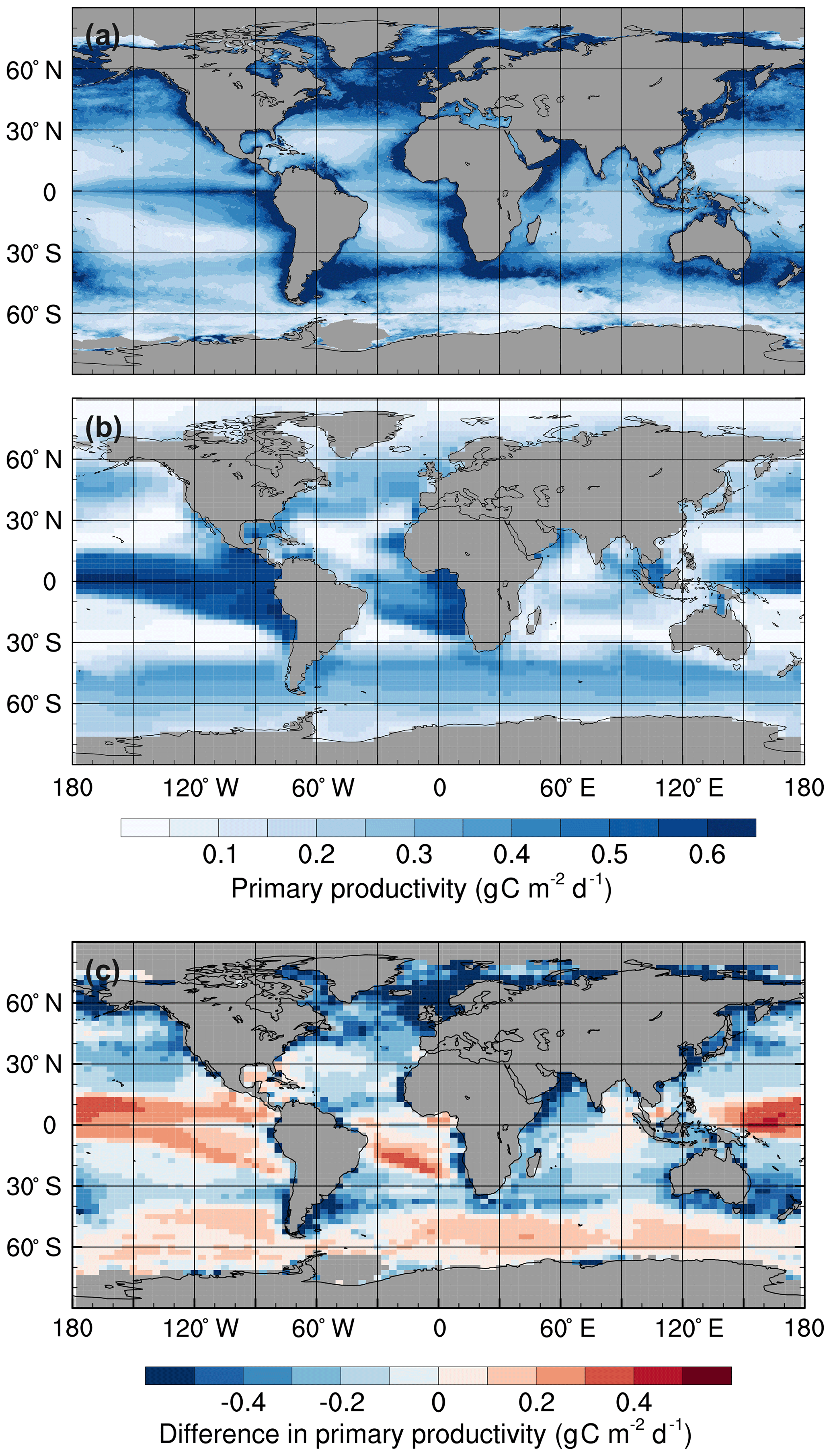
Figure 1Mean annual surface primary productivity: (a) observations estimated from surface chlorophyll concentrations using the Vertically Generalised Production Model (Behrenfeld and Falkowski, 1997), (b) the std simulation in the 1990s, and (c) simulated minus observed. Monthly mean primary productivity data were obtained from the Oregon State University Ocean Productivity website (http://www.science.oregonstate.edu/ocean.productivity, last access: 23 December 2019).
HadOCC accurately simulates low primary production in the subtropical gyres and high production in the regions with the greatest nutrient supply: the subpolar North Pacific and North Atlantic oceans, and around the Antarctic Convergence Zone (Fig. 1). However, primary production is higher than observed in the equatorial Pacific, which is attributed to excessive upwelling in the eastern equatorial Pacific (Palmer and Totterdell, 2001). Production is lower than observed northwards of 50∘ N in the Atlantic and Pacific basins because sea ice formation and melt do not affect salinity distributions (an area for future development), although the model does include an iceberg meltwater flux (Smith et al., 2008). Consequently, stably stratified, low-salinity layers of meltwater, which promote phytoplankton growth, are not represented in the model (Palmer and Totterdell, 2001). Furthermore, the simulated production in coastal regions is lower than observed. There are three main reasons for this: (1) HadOCC does not simulate riverine input of nutrients, which are a significant source of coastal nutrients; (2) most of the coastlines in FAMOUS are directly adjacent to ocean grid cells that are more than 1 km deep, which dilutes near-surface nutrient concentrations; and (3) upwelling is spread out over several grid points, which causes production to be more diffuse than observed (Palmer and Totterdell, 2001).
The level of representation of ecosystem processes in HadOCC is of intermediate complexity, making it computationally faster than more sophisticated ecosystem models that include additional POC species and/or multiple nutrients (e.g. PISCES). Previous studies have found that errors in biogeochemical simulations are largely driven by biases in the physical ocean circulation (i.e. inaccuracies in the climate or ocean model to which the ecosystem model has been coupled; Doney, 1999; Doney et al., 2004; Najjar et al., 2007). Thus, simulating carbon isotopes in a more complex ecosystem model would not necessarily yield substantially better results.
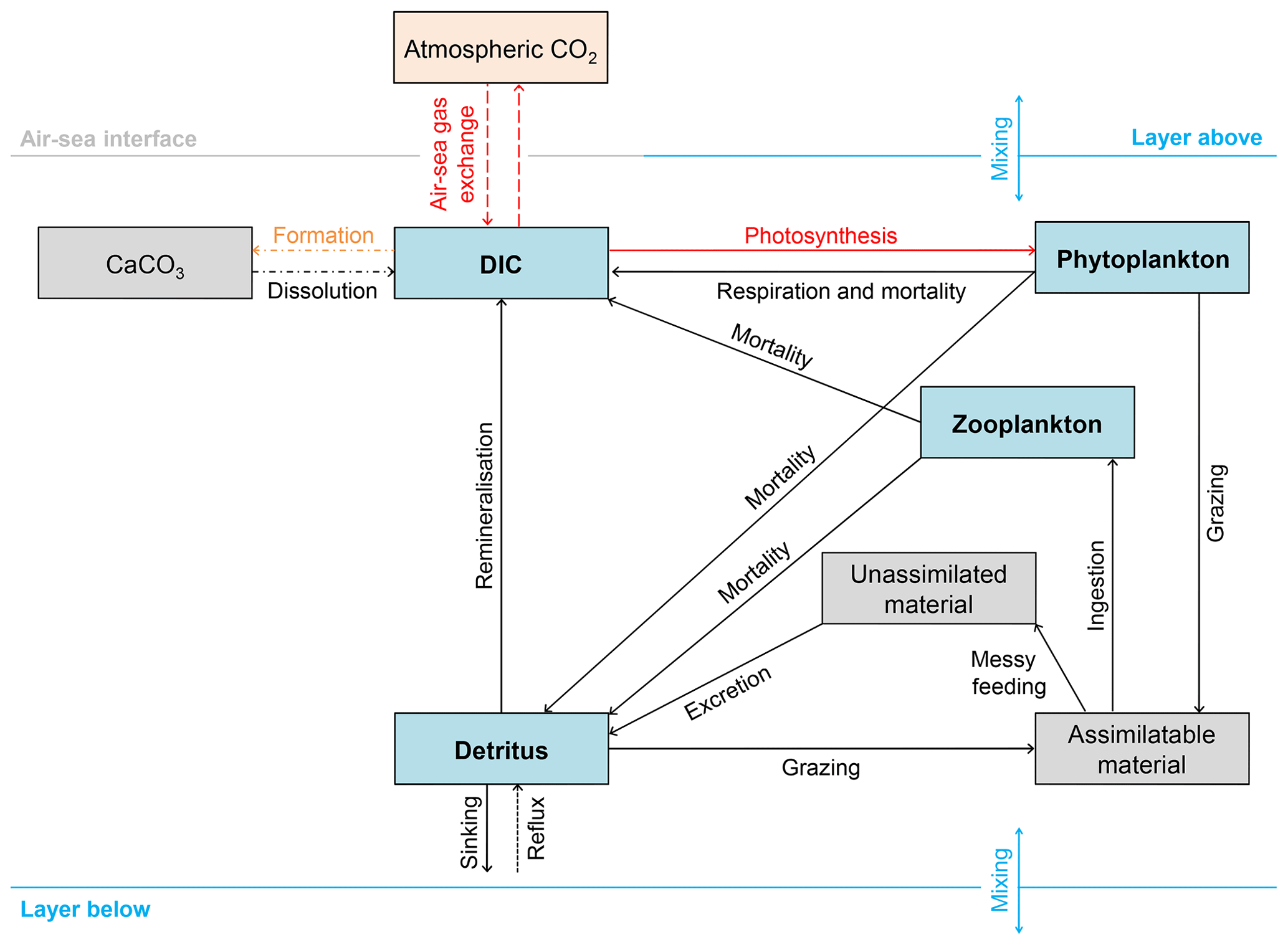
Figure 2Schematic overview of the 13C implementation in FAMOUS. Blue boxes represent permanent carbon pools. Grey boxes represent temporary carbon pools (note that CaCO3 is a temporary carbon pool because the export of CaCO3 in FAMOUS is represented as an instantaneous redistribution of alkalinity and carbon at depth). The orange box represents the prescribed atmospheric carbon pool. The dashed lines represent fluxes of 13C∕12C. However, note that the outgassed 13C∕12C has no effect on δ13Catm because FAMOUS does not currently have a fully interactive carbon cycle. Solid lines represent fluxes of 13C. Dot-dashed lines represent processes that occur below the lysocline (≈2500 m below sea level). The dotted line represents the reflux of detrital material from the seafloor to the surface layer. Red lines represent fractionation effects. The orange line represents isotopic fractionation during calcium carbonate formation (), which is included in the code as a user-specified constant. Note that all simulations presented in this study were run without fractionation during calcium carbonate formation (i.e. , which is equivalent to a fractionation effect of 0 ‰).
2.2 Carbon isotope implementation
We added 13C to the four carbon pools in HadOCC: DIC, phytoplankton, zooplankton, and detritus (Fig. 2). We assume that modelled DIC is 12C and carry 13C as a ratio (DI13C∕DI12C); therefore, virtual fluxes are not required to account for the dilution or concentration effects of surface freshwater fluxes (Appendix A). We also use model units to minimise the error associated with carrying small numbers:
where (Craig, 1957). We account for isotopic fractionation during air–sea gas exchange (Sect. 2.2.1 and Appendix B) and photosynthesis (Sect. 2.2.2 and Appendix C). Observational estimates suggest that isotopic fractionation during CaCO3 formation is between +3 ‰ and −2 ‰ (Ziveri et al., 2003), which is small compared to the other fractionation effects (Turner, 1982). Previous 13C isotope implementation studies have therefore assumed either no isotopic fractionation during CaCO3 production (Schmittner et al., 2013) or prescribed constant values, for example, +1 ‰ (Tagliabue and Bopp, 2008) or +2 ‰ (Jahn et al., 2015). We conducted sensitivity tests where fractionation during CaCO3 formation was included at constant rates of −2 ‰, 0 ‰, and +2 ‰, respectively. After 10 000 years, there was 0.001 ‰ difference in both the mean surface ocean δ13CDIC values and the surface standard deviations between all three simulations, and 0.02 ‰ difference between the three global volume-weighted integrals. Since these differences are small, we proceeded with the equivalent of no fractionation during CaCO3 production ().
2.2.1 Air–sea gas exchange
The air–sea gas flux of DI12C (F) is calculated as
where Csat is the saturation concentration of atmospheric CO2 (in mol m−3), Csurf is the surface aqueous concentration of CO2 (in mol m−3), and PV is the piston velocity (in cm h−1), which is calculated as
where a is a tuneable coefficient, u is the wind speed (in m s−1), aice is the fractional ice cover, and Sc is the Schmidt number for CO2, calculated as a function of sea surface temperature (SST, in ∘C):
The air–sea gas flux of DI13C∕DI12C is calculated as
where 13A∕12A and 13C∕12C are the 13C∕12C ratios of the atmosphere and DIC, respectively, αk is the constant kinetic fractionation factor (0.99919), αaq←g is the temperature-dependent fractionation during gas dissolution:
and αDIC←g is the temperature-dependent fractionation between aqueous CO2 and DIC:
All three fractionation factors are based on the equations of Zhang et al. (1995). However, following Schmittner et al. (2013), we neglect the effect that the carbonate fraction (fCO3) has on αDIC←g because this is much smaller (0.05 ‰) than the temperature effect (3 ‰). Currently, atmospheric CO2 and δ13C concentrations can either be held constant or prescribed from a file that contains a single global weighted-average value per year.
2.2.2 Photosynthesis
Isotopic fractionation during photosynthesis (αPOC←DIC, herein αp) is calculated as
where αPOC←aq is the equilibrium fractionation factor between aqueous CO2 and POC.
Empirical relationships for the different biogeochemical fractionation effects (αaq←g, αDIC←g, and αPOC←aq) have been established from laboratory experiments, modern oceans and lakes, and the sedimentary record. However, there are still uncertainties associated with the parameterisation of αPOC←aq. Early studies investigated a potential temperature dependence of the carbon isotope composition of marine phytoplankton. For example, Sackett et al. (1965) proposed that photosynthetic fractionation is higher at lower temperatures (0.23 ‰ per ∘C) after observing that phytoplankton in the Drake Passage had more negative δ13C values than those in the tropics. Wong and Sackett (1978) also recorded small temperature effects (−0.13 ‰ to +0.36 ‰ per ∘C) in 17 species of marine phytoplankton; however, the authors concluded that the 15 ‰ range observed in their samples was primarily related to different metabolic pathways within the organisms. Numerous studies have suggested that the fractionation of carbon isotopes during photosynthetic CO2 fixation relates to aqueous CO2 concentrations () in the ambient environment (Popp et al., 1989; Rau et al., 1989; Jasper and Hayes, 1990; Hollander and McKenzie, 1991; Freeman and Hayes, 1992). However, these studies assumed that CO2 only enters the phytoplankton by passive diffusion and neglected physiological effects, such as phytoplankton growth rate, cell size and geometry, and cell membrane permeability. Taking into consideration that physiological factors may modify, weaken, or eliminate the relationship between and photosynthetic fractionation, Rau et al. (1996) proposed a model that accounted for the isotopic composition of the ambient aqueous CO2, isotopic fractionation associated with diffusive transport into the cell, and isotopic fractionation associated with enzymatic, intracellular fixation. Laws et al. (1995) identified a linear relationship between phytoplankton growth rate, , and isotopic fractionation during photosynthesis under the assumption that the growth rate is proportional to the net transport of CO2 into the cell. A later study by Laws et al. (1997), which analysed the same species of marine diatom over a larger range of , revised this to a non-linear relationship. Burkhardt et al. (1999) and Keller and Morel (1999) additionally included active bicarbonate transport in their calculations, recognising that aqueous CO2 is not the only substrate for photosynthetic fixation and that processes other than diffusion can contribute to inorganic carbon acquisition. This has been a relatively inactive research area in the last 20 years, but there remains no single accepted model for fractionation during photosynthesis.
Consequently, previous carbon isotope implementation studies have used a number of different parameterisations for biological fractionation (Table 1), with the choice of scheme largely reflecting the complexity of the simulated biogeochemical and ecosystem processes. It is difficult to compare the success of the different parameterisations used by individual modelling groups because inter-model differences in the simulated isotopic distributions predominantly relate to resolution, complexity, and biases in the physical ocean circulation and ocean biogeochemistry, as opposed to the choice of fractionation scheme. However, Hofmann et al. (2000) tested three different fractionation schemes within a single model. In their study, the oversimplified assumption of constant biological fractionation, taken from Maier-Reimer (1993), failed to reproduce the observed latitudinal gradients in δ13CPOC. Calculating the fractionation as a function of , as per Popp et al. (1989), successfully replicated the interhemispheric asymmetry in δ13CPOC, but a growth-rate-dependent fractionation (e.g. Rau et al., 1996) was required to additionally capture the seasonal variations. Jahn et al. (2015) also demonstrated differences between three different fractionation schemes within a single model. In their study, the simple scheme of Rau et al. (1989) produced lower δ13CDIC values in the surface ocean and higher δ13CDIC values below 150 m compared to the more complex parameterisations of Laws et al. (1995) and Keller and Morel (1999). The differences between the intermediate-complexity formulation (Laws et al., 1995) and the most complex formulation (Keller and Morel, 1999) were small, and the Laws et al. (1995) equation was chosen as the default scheme.
To account for the uncertainty associated with biological fractionation in FAMOUS, we tested three different parameterisations for αPOC←aq. In the standard simulation (std), we calculated αPOC←aq according to Popp et al. (1989):
where is the aqueous CO2 concentration (in µmol L−1).
Both of the alternative parameterisations calculated αPOC←aq as a function of the phytoplankton-specific growth rate (μ) and , representing an increase in complexity relative to the standard scheme. The first was a linear relationship derived from the experimental results of Laws et al. (1995):
The second was a non-linear relationship derived from the experimental results of Laws et al. (1997):
Because HadOCC is a relatively simple ecological model, with only a single representation of phytoplankton, we did not test more complex schemes, such as those that use phytoplankton-type-specific cell parameters (e.g. Burkhardt et al., 1999; Keller and Morel, 1999).
2.2.3 Advection
The default advection scheme in FAMOUS is Quadratic Upstream Interpolation for Convective Kinematics (QUICK) with flux limiter (Leonard et al., 1993). This scheme is used to compute the transport of tracers such as temperature, salinity, nutrients, and DIC throughout the ocean. For consistency, we use the same advection scheme to calculate 13C concentrations in the ocean interior. For greater numerical stability, δ13CDIC is fixed at 0 ‰ in the Hudson Bay and Baltic Sea. With the model's standard pre-industrial land–sea mask, these inland bodies of water are isolated from the global oceans; therefore, their isotope concentrations will not affect large-scale tracer distributions.
2.3 Simulations
2.3.1 Spin-up simulation
Carbon isotope simulations must be spun up over multiple millennia (5000 to 15 000 years; Orr et al., 2000) to reach steady state because of the long timescale of deep ocean ventilation (Bardin et al., 2014). We therefore ran our spin-up simulation for 10 000 years with constant pre-industrial boundary conditions, where δ13Catm was fixed at −6.5 ‰ (Francey et al., 1999) and δ13Cocn was initialised at a globally uniform value of 0 ‰. The global volume-weighted integral of δ13CDIC started to stabilise after 7000 years, and at the end of the spin-up simulation, the drift was less than 0.001 ‰ yr−1 (Fig. S1 in the Supplement).
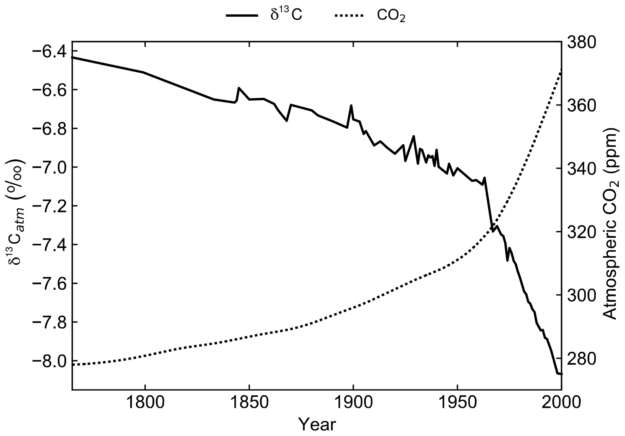
Figure 3Prescribed atmospheric δ13C values (solid) from the Law Dome and South Pole ice core records (Rubino et al., 2013) and prescribed atmospheric CO2 values (dashed) from the OCMIP-2 files (Orr et al., 2000).
2.3.2 Historical simulation
A transient simulation for the period 1765 to 2000 CE was initialised from the end of the spin-up simulation to generate model output that is directly comparable to modern observations (Fig. 3). Atmospheric CO2 concentrations were prescribed from the OCMIP-2 files (Orr et al., 2000) and δ13Catm was prescribed from the Law Dome and South Pole ice core records (Rubino et al., 2013). The decrease in δ13Catm from −6.5 ‰ in 1750 to approximately −8.0 ‰ in 2000 is due to the Suess effect. First observed in tree ring records of atmospheric composition, the Suess effect refers to the dilution of 13C in any carbon pool due to fossil fuel burning (Suess, 1955; Keeling, 1979). Fossil fuels formed millions of years ago from organic matter, which is relatively 13C depleted due to isotopic fractionation during photosynthesis. Their isotopic signature is therefore approximately 20 ‰ lower than that of the ambient atmosphere (Andres et al., 1994, 1996). To act as a control, the spin-up simulation was continued for an additional 235 years with constant CO2 and δ13Catm.
2.3.3 Sensitivity experiments
Five further simulations were conducted to quantify the effects of fractionation during air–sea gas exchange and primary productivity on the simulated δ13CDIC distributions. All five simulations were run for 10 000 years with constant pre-industrial boundary conditions. In each of the simulations, δ13Catm was fixed at −6.5 ‰ and δ13Cocn was initialised at 0 ‰. At the end of each of the spin-up simulations, the global volume-weighted δ13CDIC integral was drifting by less than 0.001 ‰ yr−1.
Table 2Overview of the fractionation factors used in the sensitivity experiments.
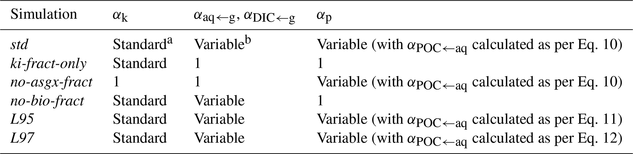
a 0.99919; b Calculated as per Eqs. (7)–(8)
Three of the simulations were designed to quantify the effects of the individual processes outlined in Sect. 2.2 (Table 2). In the ki-fract-only simulation, αaq←g, αDIC←g, and αp were all set to 1; therefore, only kinetic fractionation effects were calculated. In the no-asgx-fract simulation, αk, αaq←g, and αDIC←g were all set to 1 to eliminate the effect of fractionation during air–sea gas exchange. Fractionation during photosynthesis continued to be calculated using the std biological fractionation scheme, as per Eqs. (9)–(10). In the no-bio-fract simulation, αp was set to 1 to remove the effect of fractionation during photosynthesis, but fractionation during air–sea gas exchange continued to be calculated as per Eqs. (6)–(8).
The other two simulations were designed to assess the sensitivity of the simulated δ13CDIC distributions to the choice of biological fractionation scheme (Sect. 2.2.2). In the L95 simulation, αPOC←aq was calculated using Eq. (11), whilst in the L97 simulation, αPOC←aq was calculated using Eq. (12). As with the std simulation, we initialised a 235-year transient simulation (with the 13C-Suess effect) from the end of both of these spin-ups to allow the output from all three photosynthetic fractionation schemes to be compared directly to observations.
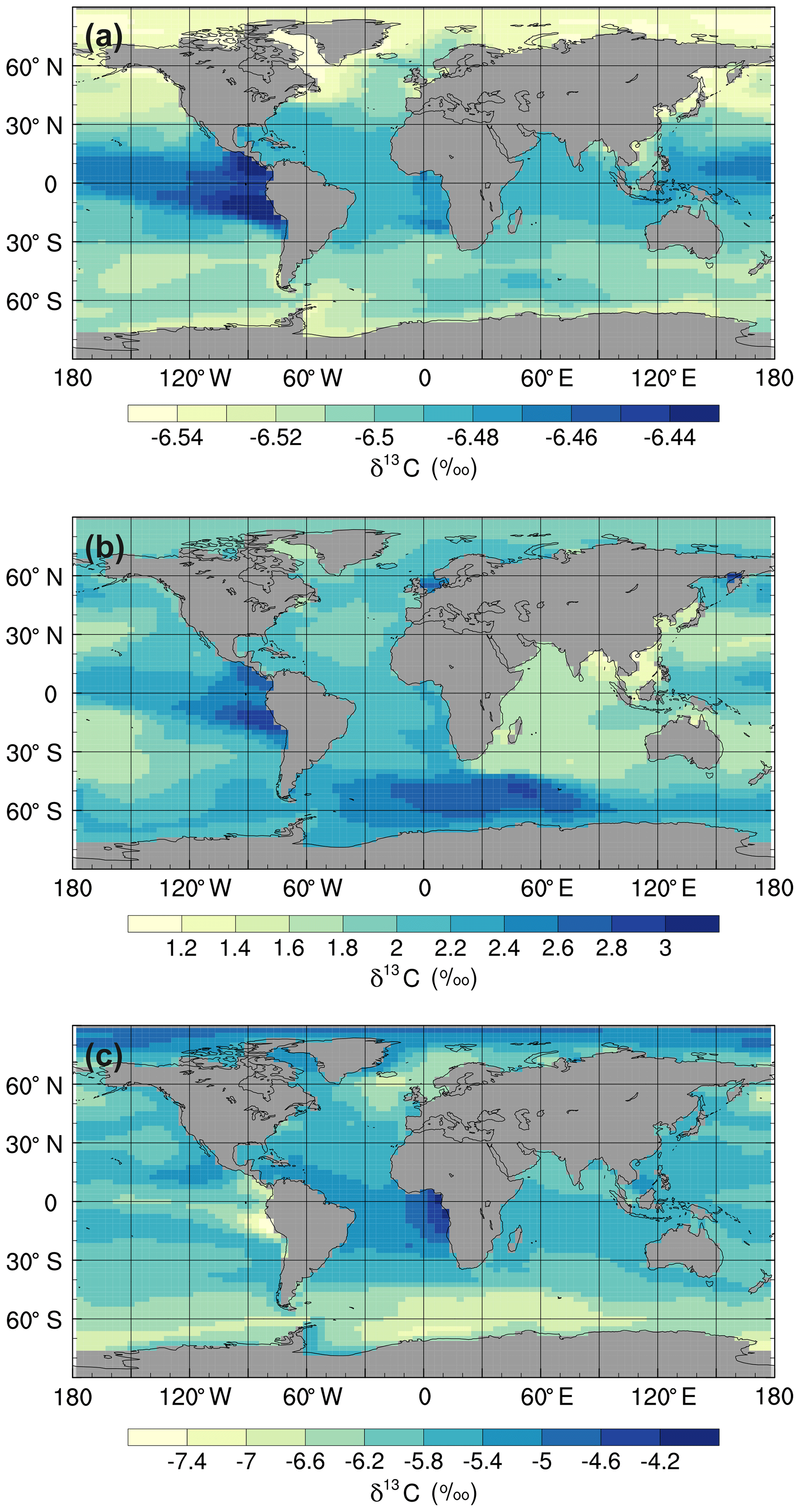
Figure 4Mean annual surface δ13CDIC values at the end of the sensitivity experiment spin-up simulations (years 9900 to 10 000): (a) ki-fract-only, (b) no-bio-fract, and (c) no asgx-fract.
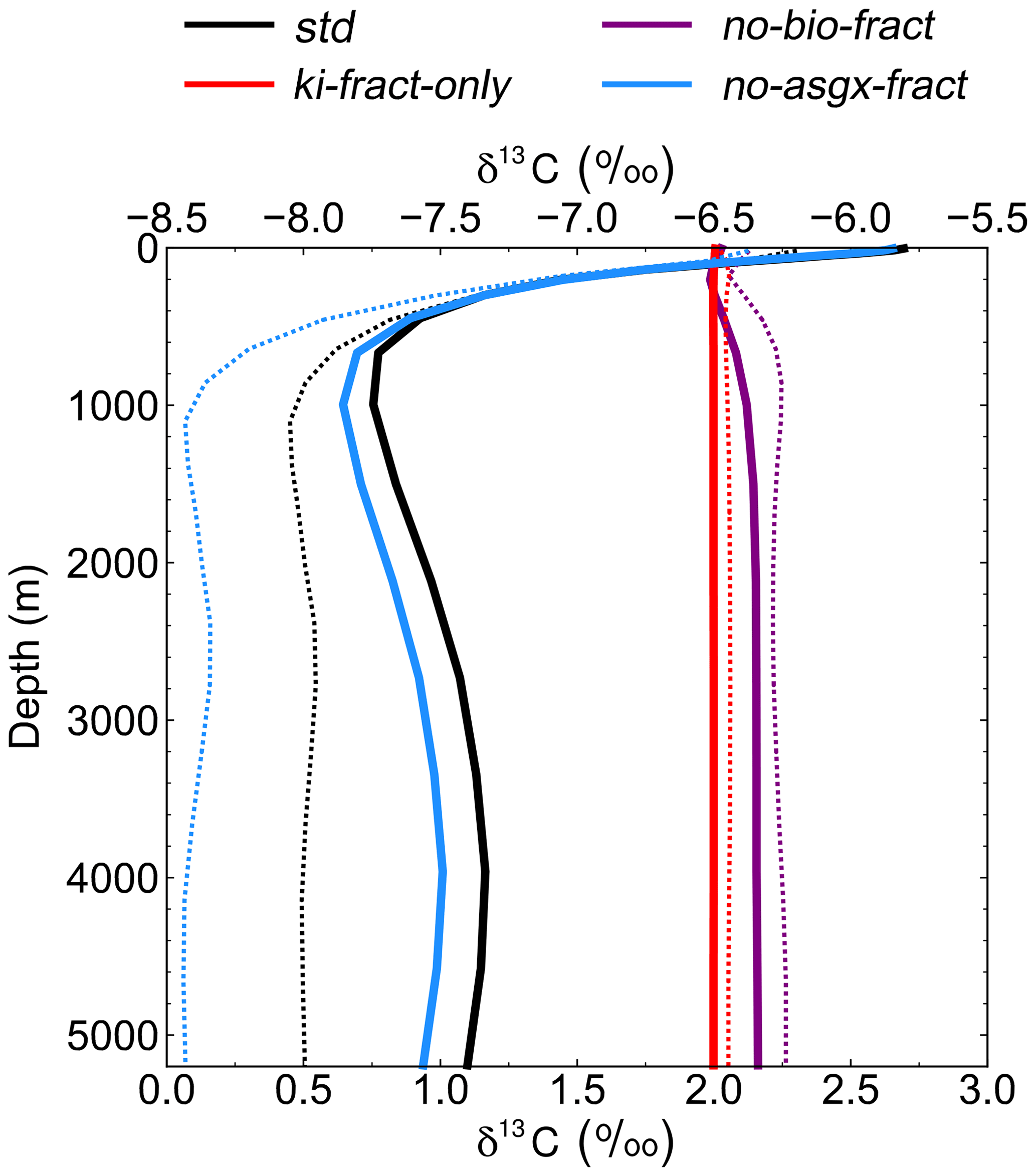
Figure 5Depth profiles of globally averaged δ13CDIC at the end of the sensitivity experiment spin-up simulations (years 9900 to 10 000). The std (black) and no-bio-fract (purple) simulations use the bottom axis, whilst the ki-fract-only (red) and no-asgx-fract (blue) simulations use the top axis. The dotted lines are the equivalent simulations conducted by Schmittner et al. (2013) with the UVic ESM: std (black) and no-bio (purple) on the bottom axis; ki-only (red) and const-gasx (blue) on the top axis.
3.1 Validating the isotope scheme
Isolating the different fractionation effects allows us to assess the relative contribution of air–sea gas exchange and biology to the simulated δ13CDIC distributions, and validate that the new isotope scheme is responding to physical and biogeochemical processes as expected. If there is no fractionation during either air–sea gas exchange or photosynthesis, the ocean equilibrates at a uniform value of −6.5 ‰, in line with the atmosphere (simulation not shown). Kinetic fractionation has only a minor effect on surface ocean δ13CDIC distributions, with simulated δ13CDIC values in the ki-fract-only simulation ranging between −6.57 ‰ in the Labrador Sea and −6.42 ‰ in the eastern equatorial Pacific (Fig. 4a). This represents a −0.07 ‰ to +0.08 ‰ shift relative to no isotopic fractionation. Specifically, there is 13C depletion (low δ13CDIC) in areas of net CO2 invasion, such as the extratropics and high latitudes, and 13C enrichment (high δ13CDIC) in the equatorial upwelling zones and the deep water formation regions where CO2 is being outgassed. Kinetic fractionation has a negligible effect on the δ13CDIC depth profile, with globally averaged δ13CDIC values of −6.4955 ‰ in the surface ocean and −6.5011 ‰ in the abyssal ocean (Fig. 5).
When both the equilibrium and kinetic fractionation effects are included during air–sea gas exchange (no-bio-fract), the large-scale δ13CDIC distributions are closely related to the SST patterns because of the temperature dependence of αaq←g and αDIC←g (Fig. 4b). In the absence of biological fractionation, relatively high δ13CDIC values ( ‰) are simulated in the Southern Ocean due to the combined effect of CO2 outgassing and low SSTs, both of which cause 13C enrichment. The δ13CDIC values in the Arctic Ocean are comparably low because the model has more extensive sea ice in the Northern Hemisphere than in the Southern Hemisphere, which inhibits air–sea gas exchange. The highest values (+3.00 ‰) are simulated in the eastern equatorial Pacific where there are high rates of net CO2 outgassing, and southern-sourced waters, which have a high δ13CDIC signature in this simulation because there is no biological fractionation, are upwelled. Low δ13CDIC values are simulated in the Indian Ocean, with the lowest values (+1.1 ‰) in southeast Asia, because the sea surface is warmer than at the equivalent latitudes in the Atlantic and Pacific oceans. The globally averaged δ13CDIC values in this simulation range between +2.03 ‰ in the surface ocean and +2.16 ‰ in the deep ocean, with a minimum value of +2.00 ‰ at a depth of approximately 200 m (Fig. 5). Below approximately 1500 m, the globally averaged δ13CDIC is near constant with depth, matching the simulated temperature profile.
When only biological fractionation effects are included (no-asgx-fract), δ13CDIC values in the surface ocean range between −7.65 ‰ in the eastern equatorial Pacific and −3.89 ‰ in the eastern equatorial Atlantic (Fig. 4c), representing a shift of −1.15 ‰ to +2.61 ‰ relative to no isotopic fractionation. The asymmetry between these two upwelling zones occurs because the waters that are being upwelled from the deep Pacific Ocean are approximately 600 years older than the equivalent waters in the Atlantic Ocean. They therefore contain a higher percentage of remineralised organic matter, which is enriched in 12C. Relatively low δ13CDIC values are also simulated in the Southern Ocean and northeast North Atlantic Ocean where older water is mixed upwards from the abyssal ocean to the surface ocean at sites of deep water formation. The globally averaged δ13CDIC values in this simulation range between −5.85 ‰ in the productive surface ocean and −7.56 ‰ in the abyssal ocean, with a minimum value of −7.86 ‰ at a depth of approximately 1000 m, which corresponds to the depth of maximum remineralisation in the model (Fig. 5). The values change from greater than −6.5 ‰ (enriched in 13C relative to no fractionation) to less than −6.5 ‰ (depleted in 13C relative to no fractionation) at a depth of approximately 100 m, which corresponds to the photic zone.

Figure 6Zonally averaged mean annual surface δ13CDIC at the end of the sensitivity experiment spin-up simulations (years 9900 to 10 000). The std (black) and no-bio-fract (purple) simulations use the left-hand axis, whilst the ki-fract-only (red) and no-asgx-fract (blue) simulations use the right-hand axis. The dotted lines are the equivalent simulations conducted by Schmittner et al. (2013) with the UVic ESM: std (black) and no-bio (purple) on the left-hand axis; ki-only (red) and const-gasx (blue) on the right-hand axis.
The spatial patterns in the std simulation and the no-asgx-fract simulation are closely matched, both in the surface ocean (Fig. 6) and at depth (Fig. 5), demonstrating the importance of biology to the large-scale δ13CDIC distributions. However, in the surface layer, air–sea gas exchange partly compensates for the biological effects in the Southern Ocean, the Northern Hemisphere deep water formation region, and the equatorial upwelling zones, as inferred from the peak surface zonal mean δ13CDIC values at 60∘ S, 55∘ N and 0∘ in the no-bio-fract simulation, which correspond with reduced amplitude troughs in the std simulation relative to the no-asgx-fract simulation. Similar results pertaining to the relative influence of air–sea gas exchange and biology were presented by Schmittner et al. (2013), who concluded that air–sea gas exchange and temperature-dependent fractionation reduce the spatial δ13CDIC gradients that are created by biology. Earlier work by Murnane and Sarmiento (2000) and Schmittner et al. (2013) also supports the notion that biology is the dominant factor controlling δ13CDIC distributions in the interior ocean. Overall, the sensitivity experiments demonstrate that the new carbon isotope scheme is accurately responding to physical and biogeochemical processes in the model, such as temperature, air–sea gas exchange, and the biological pump.
3.2 Comparison to observations
To assess the model performance in representing modern large-scale 13C distributions, we compare the simulated mean δ13CDIC values for the 1990s with observations from GLODAP version 2 (v2; Key et al., 2015; Olsen et al., 2016) and the gridded global ocean climatology of Eide et al. (2017). The δ13CDIC values in the std simulation are, on average, 0.97 ‰ higher than the GLODAPv2 observations in the surface ocean (Fig. 7) and 0.64 ‰ higher globally, with root mean square error (RMSE) values of 1.03 ‰ and 0.91 ‰, respectively. However, the simulated range in the surface ocean (3.2 ‰) is in excellent agreement with the observed range (3.3 ‰). Specifically, the simulated surface δ13CDIC values are between +1.4 ‰ and +4.6 ‰, with a mean value of +2.6 ‰, whilst the observed surface δ13CDIC values range between −0.3 ‰ and +3.0 ‰, with a mean value of +1.5 ‰.
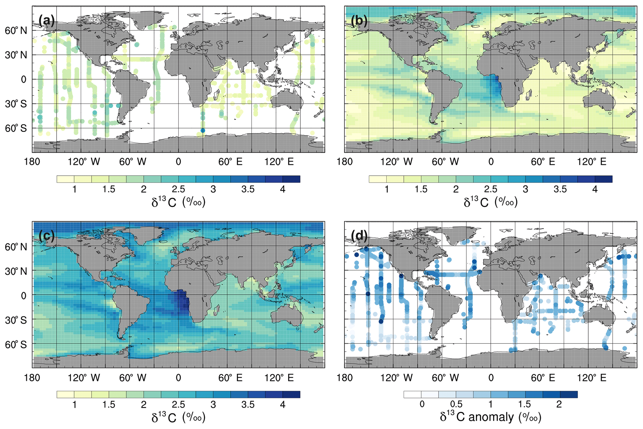
Figure 7Mean annual surface δ13CDIC during the 1990s: (a) observations from GLODAPv2 (Key et al., 2015; Olsen et al., 2016), (b) the std simulation corrected for the mean surface bias (0.97 ‰), which is calculated as ∑(simulated-observed)/number of observations, (c) the std simulation, and (d) std minus GLODAPv2.
Re-examining the results of the sensitivity experiments allows us to ascertain the underlying causes of the model–data discrepancy. Schmittner et al. (2013; herein S13) conducted a similar set of simulations with the UVic ESM to elucidate the relative influence of biology and air–sea gas exchange on the distribution of oceanic δ13CDIC (see Table 1 in S13). Overall, there is good agreement between our ki-fract-only and no-bio-fract simulations and the equivalent simulations in S13 (ki-fract and no-bio, respectively), both in the surface ocean (Fig. 6) and at depth (Fig. 5). However, there is a clear difference between the results of our no-asgx-fract simulation and the equivalent simulation in S13 (const-gasx). Specifically, the surface ocean zonal mean δ13CDIC values in our no-asgx-fract simulation range between −6.6 ‰ at 60∘ S and −5.5 ‰ in the subtropics, with a local minimum of −5.8 ‰ at the Equator (solid blue line in Fig. 6). For comparison, the surface ocean zonal mean values in const-gasx range between −8.0 ‰ in the Southern Ocean and −5.75 ‰ in the Southern Hemisphere subtropics, with a localised minimum of −6.25 ‰ at the Equator (dotted blue line in Fig. 6). Similarly, whilst the globally averaged deep ocean δ13CDIC values in our no-asgx-fract simulation have a comparable range (2.01 ‰) to the deep ocean values in const-gasx, there is an offset of approximately 1 ‰, with S13 simulating δ13CDIC values of −6.4 ‰ in the surface ocean, −8.4 ‰ in the deep ocean, and near constant values below 1000 m (blue lines in Fig. 5). Overall, the δ13CDIC values in the standard simulation with the UVic ESM are in good agreement with observations, with a global linear regression r2 value of 0.91 and a global RMSE of 0.33 ‰ (Schmittner et al., 2013; Buchanan et al., 2019). We therefore postulate that the offset in the simulated δ13CDIC values in FAMOUS relates to biases in the biological carbon cycle.
Elucidating the exact cause of δ13CDIC model–data discrepancy is difficult. There are a number of fluxes going into and out of the DI13C pool (Fig. 2), each of which could have biases that are compounding or reducing the overall δ13CDIC bias. For example, if any of the rates of phytoplankton respiration, phytoplankton mortality, or zooplankton mortality are too low, the input of 12C-enriched material back into the DIC pool would be insufficient. Similarly, if the model is not simulating enough remineralisation, either as a direct consequence of the parameterised remineralisation rate or as a result of insufficient POC export, the input of 12C-enriched material back into the DIC pool would again be too low.
Primary producers preferentially take up 12C during photosynthesis; therefore, higher-than-observed rates of net primary production in the photic zone would increase δ13CDIC. However, if the δ13CDIC discrepancy in FAMOUS was a simple function of the biases in net primary production, δ13CDIC would be lower than observed in the subtropical gyres, the Indian Ocean, and the northern North Atlantic and North Pacific oceans, and higher than observed in the equatorial upwelling zones and the Southern Ocean (Fig. 1). Thus, whilst the differences in net primary production could be contributing towards the δ13CDIC bias, particularly in the equatorial upwelling zones, they alone cannot explain the unidirectional offset.
Alternatively, the fractionation during photosynthesis could be too strong as a result of imbalances in the carbonate chemistry (Fig. S2). The global mean alkalinity in FAMOUS is 81 µmol kg−1 higher than observed and the mean alkalinity in the uppermost 50 m of the ocean is 107 µmol kg−1 too high (Key et al., 2004; Sarmiento and Gruber, 2006). In addition, the simulated global mean DIC concentration is 54 µmol kg−1 higher than observed and the mean DIC concentration in the uppermost 50 m of the ocean is 96 µmol kg−1 too high (Key et al., 2004; Sarmiento and Gruber, 2006). Furthermore, the mean ocean temperatures in FAMOUS are warmer than observed, both globally (2.2 ∘C) and in the uppermost 50 m of the ocean (1 ∘C; Sarmiento and Gruber, 2006; Locarnini et al., 2013). Increasing alkalinity increases , whilst increasing the temperature and DIC concentrations decreases . Hence, the overall effect of the carbonate chemistry biases in FAMOUS result in the global mean being 3.03 µmol L−1 too low and the mean in the uppermost 50 m of the ocean being 0.58 µmol L−1 too high. In the photic zone, this translates to a simulated αp of 0.97378 compared to an observed αp of 0.97415 using the std fractionation parameterisation. Thus, we postulate that imbalances in the carbonate chemistry, and the consequent differences in αp, are contributing towards the δ13CDIC bias, but the overall effect is small.
The smallest model–data discrepancies in the surface layer are in the Southern Ocean and the northeast North Atlantic Ocean where deep convection mixes 12C-enriched waters upwards (Fig. 7). In contrast, in the equatorial upwelling zones, the effect of higher than observed primary productivity (increasing δ13CDIC) outweighs the effect of vertical mixing (reducing δ13CDIC); therefore, the overall model–data biases are higher in these regions. Despite the global offset, the model correctly simulates lower δ13CDIC values in the Indian Ocean compared to the Atlantic and Pacific oceans, because the Indian Ocean is relatively nutrient poor, both in the model and reality (Fig. S3), which limits primary productivity (Fig. 1). Similar to previous 13C modelling studies (e.g. Hofmann et al., 2000; Tagliabue and Bopp, 2008; Schmittner et al., 2013), FAMOUS also accurately simulates the observed latitudinal gradient in mixed layer δ13CPOC, with relatively high values ( ‰) in the low latitudes and relatively low values ( ‰) at high latitudes (Fig. 8).
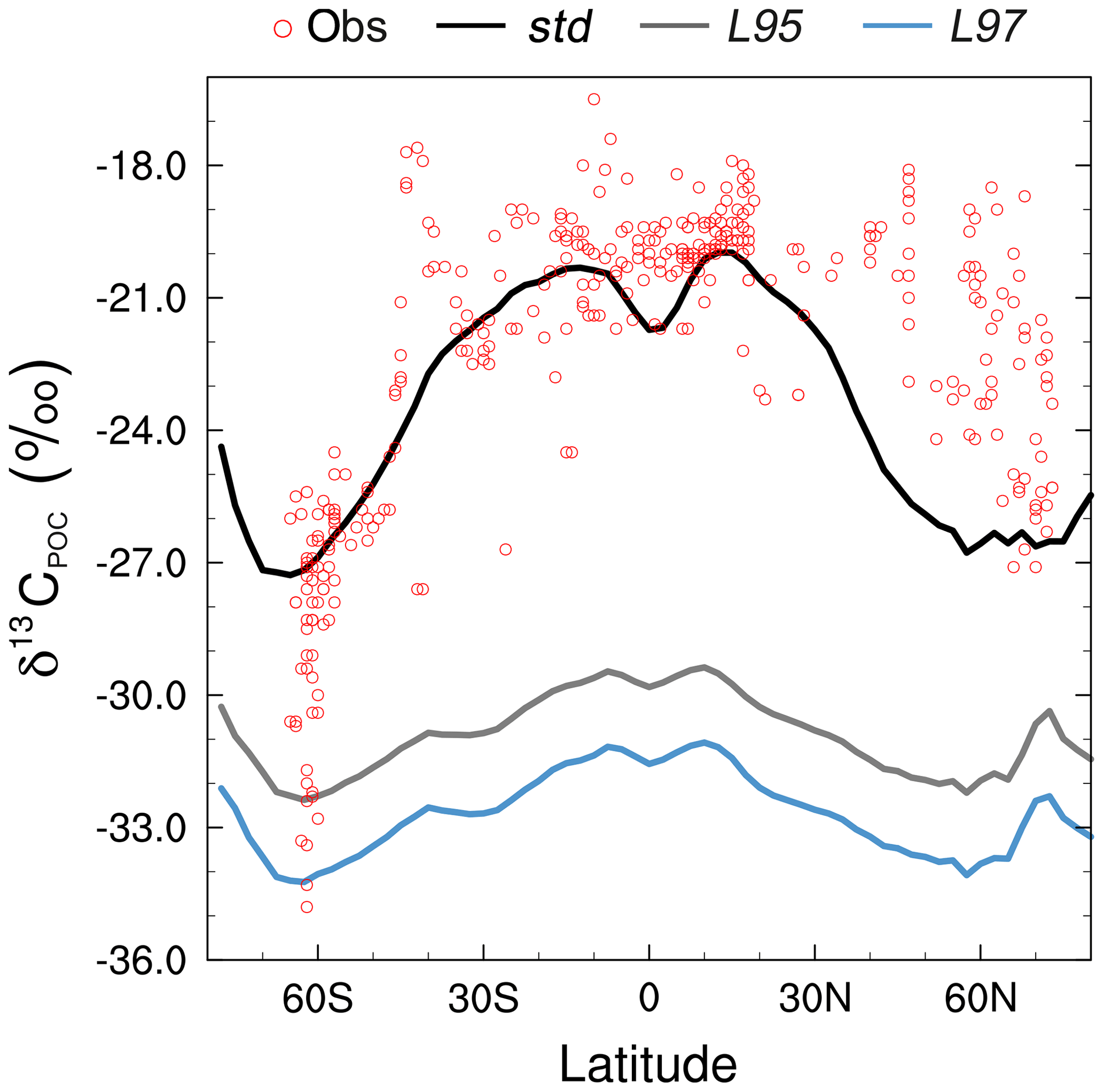
Figure 8Zonally averaged mean annual mixed layer δ13CPOC during the 1990s: observations (Goericke and Fry, 1994; red), the std simulation (black), the L95 simulation (grey), and the L97 simulation (blue).
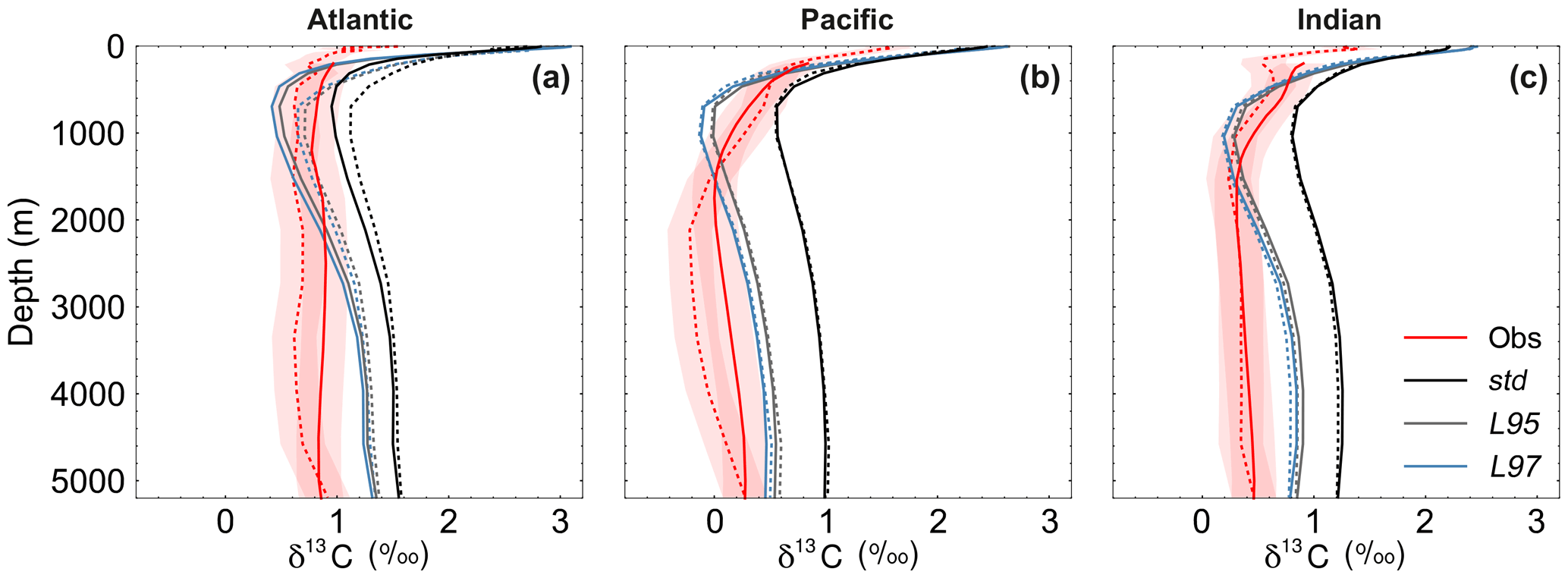
Figure 9Depth profiles of δ13CDIC during the 1990s: (a) Atlantic Ocean, (b) Pacific Ocean, and (c) Indian Ocean. The δ13CDIC values in the std (black), L95 (grey) and L97 (blue) simulations are compared to observations (red). Solid lines are used for the global dataset, with observations from the gridded climatology produced by Eide et al. (2017). The simulated values have also been subsampled at the locations where there is a corresponding observation in the GLODAPv2 dataset (Key et al., 2015; Olsen et al., 2016; dashed). The red shading shows the estimated uncertainty in δ13CDIC observations due to unresolved intercalibration between different laboratories (±0.2 ‰; Schmittner et al., 2013; Eide et al., 2017).
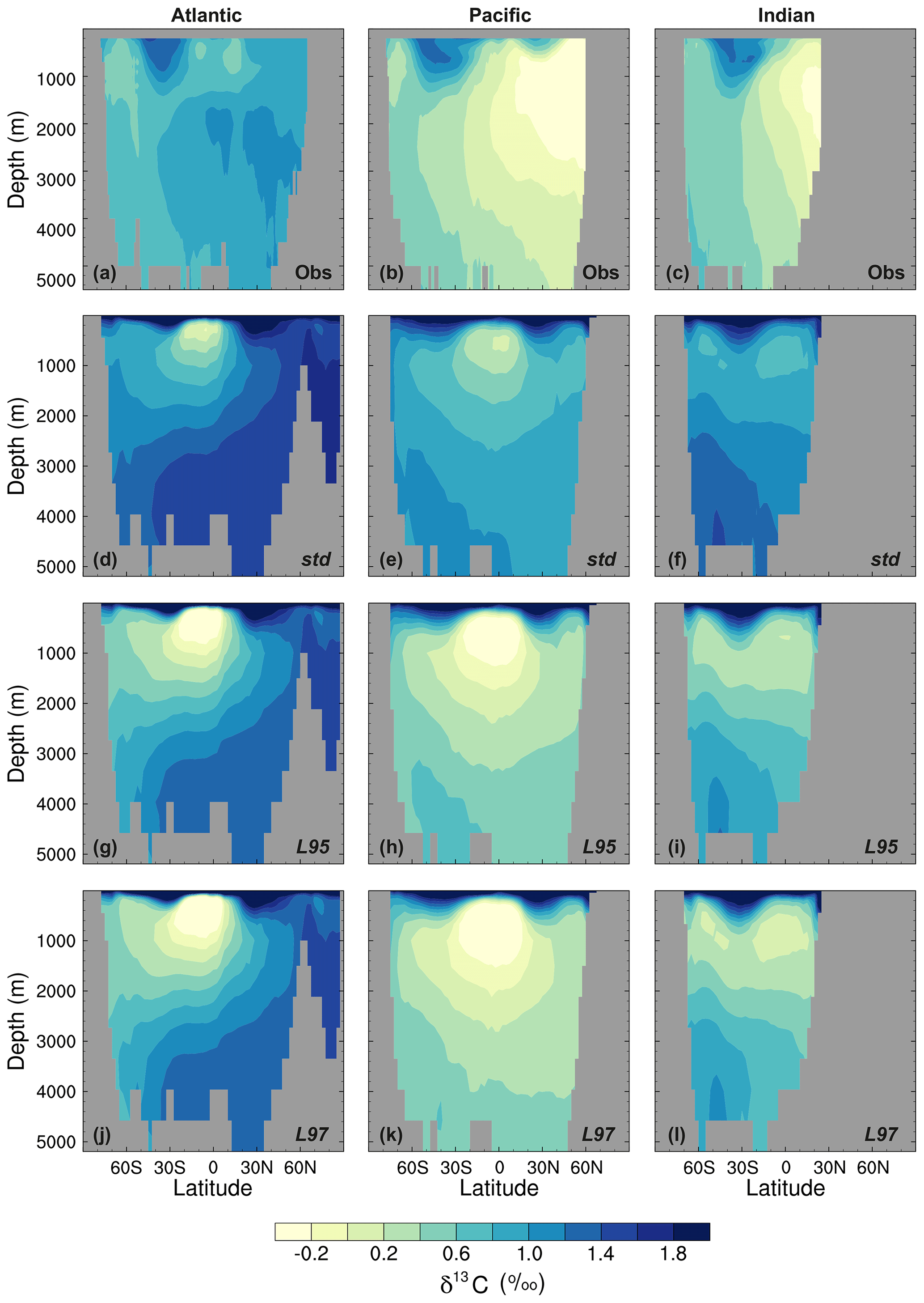
Figure 10Zonal mean δ13CDIC during the 1990s in the Atlantic Ocean (left), Pacific Ocean (centre), and Indian Ocean (right): (a–c) gridded observations (Eide et al., 2017), (d–f) the std simulation, (g–i) the L95 simulation, and (j–l) the L97 simulation.
As observed, δ13CDIC decreases with depth in all basins due to the remineralisation of isotopically light organic matter (Fig. 9). The maximum remineralisation depth in the model is approximately 1000 m, which is 200 to 500 m shallower than observed. In the deep ocean, the highest δ13CDIC values are in the Atlantic basin, with intermediate values in the Indian basin, and the lowest values in the Pacific basin, where the waters are older and therefore contain more remineralised organic material (enriched in 12C). However, there are notable structural differences in the zonal means (Fig. 10), which arise due to inaccuracies in the physical ocean circulation in FAMOUS. Specifically, FAMOUS does not capture the observed structure in the Atlantic basin because, in this generation of the model, the AMOC is characterised by an overdeep North Atlantic Deep Water (NADW) cell and insufficient Antarctic Bottom Water formation (Dentith et al., 2019b). FAMOUS also simulates weak (less than 3 Sv) ventilation to depths of 2000 m in the North Pacific Ocean (Dentith et al., 2019b), which prevents the accumulation of old, 12C-enriched (low δ13CDIC) waters at intermediate depths in the Northern Hemisphere. Instead, the oldest carbon in the model is in the eastern equatorial Pacific. In addition, the surface winds in the model are weaker than observed (Kalnay et al., 1996), resulting in a relatively shallow mixed layer. This promotes the excessive accumulation of high δ13CDIC values in the surface ocean, which is particularly notable in the Southern Hemisphere subtropical gyres. These physical model biases are also clearly visible in the zonal mean profiles of other tracers, such as nutrients (Fig. S4) and DIC (Fig. S5). The overall shape of the simulated depth profile reaffirms the notion that there are inaccuracies in both the physical and biogeochemical components of the model (Fig. 9). Below approximately 1000 m, the simulated δ13CDIC values increase with depth in each ocean basin, whilst the observed basin averages are near constant with depth. The offset between the simulated and observed values is greatest in the deep Atlantic Ocean, where too much 13C-enriched water from the shallow ocean is being circulated into the abyssal ocean. However, the trend towards increasing δ13CDIC with depth could also be in part explained by insufficient remineralisation in the model. This is supported by lower-than-observed nutrient concentrations in the deep ocean (Fig. S4). HadOCC's global export ratio at 2000 m is within the observed range, but a lack of spatial variation means that the geographic distributions are partially incorrect (Palmer and Totterdell, 2001). Hence, we postulate that localised inaccuracies in the export ratio, together with deficiencies in the parameterisation of the remineralisation rate, are contributing towards the δ13CDIC offset. The basin-averaged δ13CDIC bias is smallest in the Pacific Ocean, where the waters are old and therefore have had more time to remineralise, thereby partially compensating for the biogeochemical biases. Indeed, the shape of the simulated and observed basin-averaged depth profiles are in good agreement below approximately 2000 m in the Pacific Ocean, despite the structural differences in the zonal mean.
As outlined in Sect. 3.1, our carbon isotope implementation is sensitive to physical and biogeochemical processes in the model. Thus, whilst biases in the overturning circulation and the biological pump are currently limiting the model's ability to accurately represent modern large-scale 13C distributions, the model–data agreement could be improved if the physical and ecological components of FAMOUS were recalibrated. This will be discussed further in Sect. 3.4.
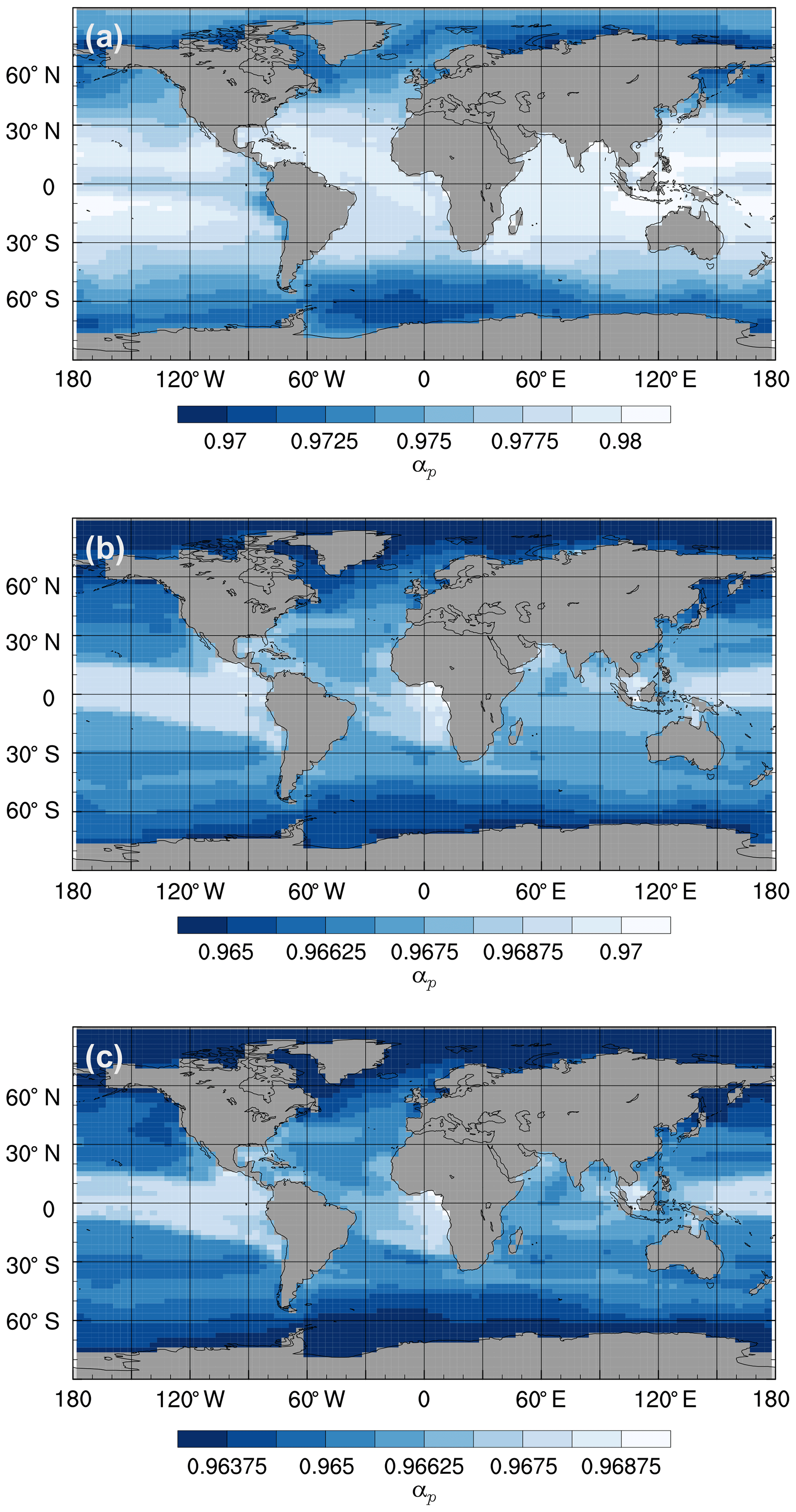
Figure 11Mean annual isotopic fractionation during photosynthesis (αp) in the surface ocean at the end of the spin-up simulations (years 9900 to 10 000): (a) the std simulation, (b) the L95 simulation, and (c) the L97 simulation.
3.3 Biological fractionation parameterisations
Given the uncertainty associated with biological fractionation (Sect. 2.2.2), we tested three different parameterisations for equilibrium fractionation during photosynthesis. For all three parameterisations, the total fractionation during photosynthesis is greatest in the high latitudes (where SSTs are relatively low and is relatively high) and lowest in the equatorial regions (where SSTs are relatively high and is relatively low; Fig. 11). The std parameterisation produces the largest range of αp values (between approximately 0.97 and 0.98), whilst the L95 parameterisation produces the smallest range (between approximately 0.964 and 0.970). The total fractionation during photosynthesis increases with the complexity of the parameterisation, with L97 producing the largest overall effect (with a minimum αp of 0.9635). For all three parameterisations, αp decreases (i.e. the strength of fractionation increases) with depth in the photic zone, with the largest gradient produced by the std parameterisation (Fig. S6).
The large-scale δ13CDIC patterns are very similar for all three photosynthetic fractionation schemes, but the parameterisations that take the phytoplankton growth rate in account simulate higher surface ocean δ13CDIC values everywhere except in the Southern Ocean, the Nordic Seas, and the eastern equatorial regions, where older 13C-depleted waters are mixed upwards from the abyssal ocean during deep water formation and upwelling (Fig. S7). The differences are amplified when using the L97 parameterisation (RMSE=1.24 ‰, bias =1.15 ‰), which specifies a non-linear relationship between μ and , compared to the L95 parameterisation (RMSE=1.21 ‰, bias=1.13 ‰), which specifies a linear relationship (Fig. S8). Conversely, the alternative parameterisations decrease δ13CDIC at depth compared to the std simulation, bringing the simulated values closer to the observations (Fig. 9). Below approximately 500 m depth, the δ13CDIC values are consistently lower when using the L97 parameterisation compared to the L95 parameterisation. This is due to the preconditioning of δ13CDIC and δ13CPOC as a result of fractionation during photosynthesis in the photic zone. In the L95 and L97 simulations, δ13CPOC is lower than in the std simulation due to increased uptake of 12C during primary production (lower αp). The latitudinal δ13CPOC gradients in the mixed layer in these simulations are lower than observed, with zonal mean values ranging between approximately −30 ‰ at the Equator and −33 ‰ at 60∘ N/S (Fig. 8). When the POC is remineralised, a relatively low δ13C signal is therefore being released back into the DIC pool, which causes the δ13CDIC in the deep ocean to be lower than in the std simulation. Thus, although the rates of biological exchange and overturning circulation are the same in all three simulations, the preconditioning of δ13CDIC and δ13CPOC in the photic zone creates differences between the three simulations at depth. Whilst the global RMSE compared to the GLODAPv2 dataset is lower in the L95 and L97 simulations (0.86 ‰ and 0.87 ‰, respectively), it is still almost double the RMSE in other models (Buchanan et al., 2019). Overall, increasing the complexity of the fractionation scheme does not significantly improve the model–data agreement because of the aforementioned physical and biogeochemical biases.
3.4 A new tuning target
In contrast with earlier studies, we have demonstrated that the new carbon isotope scheme in FAMOUS is sensitive to both physical and biogeochemical processes. The simulated δ13CDIC distributions reflect known physical inaccuracies (such as overdeep NADW and weak convection in the subpolar North Pacific Ocean) and have allowed us to identify previously undisclosed biogeochemical biases (e.g. in the representation of remineralisation). The new tracer therefore offers excellent potential as a holistic tuning target for recalibrating FAMOUS in the future.
FAMOUS has previously been tuned both systematically (Jones et al., 2005; Gregoire et al., 2011; Williams et al., 2013) and manually (Smith et al., 2008). Most recently, Williams et al. (2013) tuned the 20 structural parameters in HadOCC (coupled to FAMOUS-MOSES2.2) using an objective hypercube technique. Specifically, the parameter set included the C:N ratios for the different carbon pools, phytoplankton-specific parameters (e.g. maximum rate of photosynthesis), zooplankton-specific parameters (e.g. linear and quadratic zooplankton mortality rates), detritus-specific parameters (e.g. shallow and deep remineralisation rates), and carbonate-specific parameters (e.g. calcite export ratio). The main diagnostics used to evaluate the performance of the ensemble members were December–January–February and June–July–August surface air temperatures, annual mean total precipitation rate, annual mean nitrate concentrations, and primary productivity. Crucially, this study only ran each perturbed parameter simulation for 200 years and neglected to evaluate the strength and structure of the AMOC. The optimal parameter set therefore had small but important imbalances in the surface climate, which caused the AMOC to collapse over longer (multi-millennial) timescales (Dentith et al., 2019b).
HadOCC has not yet been tuned for the configuration of the model used in our study (FAMOUS-MOSES1). Simultaneously recalibrating HadOCC and the physical ocean circulation in FAMOUS-MOSES1 could therefore improve the simulated δ13CDIC distributions. In the first instance, further sensitivity studies would provide more insight into the extent to which our results could be improved by small adjustments to the model's biogeochemistry (e.g. modifying the remineralisation rate and/or the export ratio). Longer term, we propose that the addition of carbon isotope ratios as tuning targets (both the δ13C presented here and the new Δ14C tracer for FAMOUS discussed by Dentith et al., 2019a) would improve the work of Williams et al. (2013) because they provide an objective and straightforward way of assessing whether the balance between all of the ecological processes in the model is correct.
We have added the stable isotope 13C to the ocean component of the FAMOUS GCM, using the MOSES1 generation of the model to validate our scheme. We account for fractionation during air–sea gas exchange and photosynthesis, and have tested three different parameterisations for the latter. The model captures the range of observed δ13CDIC values in the surface ocean, but the simulated values are approximately 1 ‰ too high at all depths. The differences between the three fractionation schemes are relatively minor, but when fractionation during photosynthesis accounts for phytoplankton growth rates as opposed to just aqueous CO2 concentrations the discrepancies between the model and observations are further increased in the surface ocean and reduced at depth. The sensitivity experiments suggest that the simulated values are too high because of underlying biases in the biological carbon cycle; therefore, retuning HadOCC could improve the model–data agreement. Biases in the large-scale ocean circulation also inhibit the model's ability to accurately simulate the large-scale distribution of tracers in the deep ocean. Retuning the ocean circulation to improve the representation of the AMOC, in particular, would further reduce the model–data discrepancies. Thus, our results emphasise the utility of implementing carbon isotopes in GCMs; the simulated isotope distributions provide an additional measure against which the physical and biogeochemical model performance can be evaluated and offer an extra tuning metric for prospective development work. In the future, we intend to use the isotope-enabled model to study ocean circulation and the marine carbon cycle in both a modern and palaeo context, for example, at the Last Glacial Maximum (21 000 years ago) and during the last deglaciation (21 000 to 11 000 years ago).
The standard equation for calculating the virtual flux to account for the dilution or concentration effect of surface freshwater fluxes is
where E is evaporation, P is precipitation, and dz is layer depth.
As we carry 13C as a ratio (13C∕12C), virtual fluxes are not required:
The standard equation for calculating the change in DI13C due to air–sea gas exchange is
where PV is the piston velocity (Eq. 4), Csat is the saturation concentration of atmospheric CO2 (in mol m−3), Csurf is the surface aqueous concentration of CO2 (in mol m−3), αk is the constant kinetic fractionation factor, αaq←g is the temperature-dependent fractionation during gas dissolution (Eq. 7), αDIC←g is the temperature-dependent fractionation between aqueous CO2 and DIC (Eq. 8), and 13A∕12A and 13C∕12C are the 13C∕12C ratios of the atmosphere and DIC, respectively.
The equation for calculating the change in DI13C∕DI12C due to air–sea gas exchange is
For consistency with the standard biological tracers, the 13C contents of phytoplankton (13P), zooplankton (13Z), and detritus (13D) are carried in mmol N m−3, with the carbon concentrations and fluxes calculated using fixed stoichiometric ratios. The DI13C∕DI12C values are therefore converted from a ratio in model units (Eq. 2) to normalised DI13C concentrations before entering the soft tissue pump. The conversion is reversed at the end of each time step.
C1 Phytoplankton (P)
The standard equation for calculating the change in phytoplankton (12P) is
where RP is the specific growth rate of phytoplankton, GP represents grazing by zooplankton, mP represents phytoplankton mortality due to overpopulation, and ηP represents phytoplankton respiration.
The equation for calculating the change in 13P is
where αp is the isotopic fractionation that occurs during photosynthesis (Eq. 9), 13C∕12C is the 13C∕12C ratio of DIC, and 13P∕12P is the 13C∕12C ratio of phytoplankton. The 13P tracer is updated using the forward Euler method:
C2 Zooplankton (Z)
The standard equation for calculating the change in zooplankton (12Z) is
where βP and βD are the assimilation efficiencies associated with zooplankton grazing on phytoplankton (GP) and detritus (GD), respectively, and mZ represents zooplankton mortality due to predation and natural causes.
The equation for calculating the change in 13Z is
where 13P∕12P, 13D∕12D, and 13Z∕12Z are the isotopic ratios of phytoplankton, detritus and zooplankton, respectively.
The 13Z tracer is updated using the forward Euler method:
C3 Dissolved inorganic carbon (DIC, C)
The standard equation for calculating the change in DI12C is
where RP is the specific growth rate of phytoplankton, λD is detrital remineralisation, which is specified at a constant rate (0.1 d−1 in the uppermost 250 m of the ocean and 0.02 d−1 at all other depths), βP and βD are the assimilation efficiencies associated with zooplankton grazing on phytoplankton (GP) and detritus (GD), respectively, mZ represents zooplankton mortality due to predation and natural causes, mP represents phytoplankton mortality due to overpopulation, and ηP represents phytoplankton respiration.
The equation for calculating the change in DI13C is
where αp is the isotopic fractionation that occurs during photosynthesis (Eq. 9), and 13C∕12C, 13D∕12D, 13P∕12P, and 13Z∕12Z are the isotopic ratios of DIC, detritus, phytoplankton, and zooplankton, respectively.
The DI13C tracer is updated using the forward Euler method:
C4 Detritus (D)
Unlike the other biological tracers, the standard detritus tracer (12D) is updated using a semi-implicit scheme:
where t is the current time step, k is the model level, dD∕dtbio is the change in detritus due to biological effects (Eq. C19), γ is the sinking rate, which is parameterised at 10 m d−1, dz is the depth of the layer (in cm), and D is the detritus concentration.
Following the same principles, the 13D tracer is updated using
C4.1 Biological effects
The standard equation for calculating the change in detritus (12D) due to biology is
where mZ represents zooplankton mortality due to predation and natural causes, mP represents phytoplankton mortality due to overpopulation, λD is detrital remineralisation, which is specified at a constant rate (0.1 d−1 in the uppermost 250 m of the ocean and 0.02 d−1 at all other depths), and βP and βD are the assimilation efficiencies associated with zooplankton grazing on phytoplankton (GP) and detritus (GD), respectively.
The equation for calculating the change in 13D due to biology is
where 13Z∕12Z, 13P∕12P, and 13D∕12D are the isotopic ratios of zooplankton, phytoplankton, and detritus, respectively.
C4.2 Reflux
The small amount of detritus that reaches the ocean floor is immediately refluxed back to the surface layer to conserve nitrogen and carbon.
where k is the model level, γ is the sinking rate, which is parameterised at 10 m d−1, dz is the depth of the layer (in cm), D is the detritus concentration, and KMT is the maximum depth of the ocean. The same equation applies for 13D.
FAMOUS can be obtained from http://cms.ncas.ac.uk/wiki/UmFamous (last access: 23 December 2019). The code detailing the advances described in this paper is available via the Research Data Leeds Repository (Dentith, 2019, https://doi.org/10.5518/621) under a Creative Commons Attribution 4.0 International (CCBY 4.0) license. These files are known as code modification (“mod”) files and should be applied to the original model code, which can be viewed online at http://cms.ncas.ac.uk/code_browsers/UM4.5/UMbrowser/index.html (last access: 23 December 2019). All of the additional modification files that are required to run the simulations described in this paper are available in the Supplement. These standard FAMOUS updates – some of which have been described by Smith et al. (2008), Smith (2012), and Valdes et al. (2017) – and the original model code are protected under UK Crown Copyright. The UM configuration (“basis”) files for the simulations described in this paper are also available in the Supplement.
The simulations described in this study, as denoted by their unique five-letter Met Office UM identifiers and the notation used within this paper, are as follows:
-
XOAVB: std spin-up (0 to 10 000 years)
-
XOAVI: std transient (1765 to 2000 CE)
-
XOGNC: std control (1765 to 2000 CE)
-
XOAVD: ki-fract-only (0 to 10 000 years)
-
XOAVE: no-bio-fract (0 to 10 000 years)
-
XOAVF: no-asgx-fract (0 to 10 000 years)
-
XOAVK: L95 spin-up (0 to 10 000 years)
-
XOAVU: L95 transient (1765 to 2000 CE)
-
XOAVL: L97 spin-up (0 to 10 000 years)
-
XOAVW: L97 transient (1765 to 2000 CE)
The data are available via the Research Data Leeds Repository (https://doi.org/10.5518/621, Dentith, 2019).
The supplement related to this article is available online at: https://doi.org/10.5194/gmd-13-3529-2020-supplement.
RFI designed and supervised the project. JED wrote and implemented the code with input from JCT, LJG, and RFI. JED ran the simulations, analysed the results, and prepared the manuscript with input from all co-authors.
The authors declare that they have no conflict of interest.
Numerical climate model simulations made use of the N8 High Performance Computing (HPC) Centre of Excellence (N8 consortium and EPSRC grant no. EP/K000225/1) and ARC2, part of the HPC facilities at the University of Leeds, UK. We thank Alexandra Jahn (University of Colorado) for helpful discussions about implementing carbon isotopes in GCMs and Robin Smith (University of Reading) for the supplying code used to cap the oceanic CO2 flux. We are also grateful to Guy Munhoven and two anonymous reviewers for helping to refine the manuscript.
Jennifer E. Dentith was funded by the Natural Environment Research Council (NERC) SPHERES Doctoral Training Partnership (grant no. NE/L002574/1). Ruza F. Ivanovic acknowledges support from NERC grant NE/K008536/1. Lauren J. Gregoire was funded by a UKRI Future Leaders Fellowship (MR/S016961/1). The contribution of Julia C. Tindall was supported through the Centre for Environmental Modelling And Computation (CEMAC), University of Leeds. Laura F. Robinson acknowledges support from NERC grant R100372-101.
This paper was edited by Guy Munhoven and reviewed by two anonymous referees.
Andres, R., Boden, T., and Marland, G.: Annual Fossil-Fuel CO2 Emissions: Global Stable Carbon Isotopic Signature, CDIAC, https://doi.org/10.3334/CDIAC/FFE.DB1013.2017, 1996.
Andres, R. J., Marland, G., Boden, T., and Bischof, S.: Carbon dioxide emissions from fossil fuel consumption and cement manufacture, 1751–1991; and an estimate of their isotopic composition and latitudinal distribution, Oak Ridge National Lab., TN (United States), Oak Ridge Inst. for Science and Education, TN (United States), available at: https://www.osti.gov/biblio/10185357 (last access:29 October 2018), 1994.
Bardin, A., Primeau, F., and Lindsay, K.: An offline implicit solver for simulating prebomb radiocarbon, Ocean Model., 73, 45–58, https://doi.org/10.1016/j.ocemod.2013.09.008, 2014.
Behrenfeld, M. J. and Falkowski, P. G.: Photosynthetic rates derived from satellite-based chlorophyll concentration, Limnol. Oceanogr., 42, 1–20, https://doi.org/10.4319/lo.1997.42.1.0001, 1997.
Bouttes, N., Roche, D. M., Mariotti, V., and Bopp, L.: Including an ocean carbon cycle model into iLOVECLIM (v1.0), Geosci. Model Dev., 8, 1563–1576, https://doi.org/10.5194/gmd-8-1563-2015, 2015.
Brovkin, V., Bendtsen, J., Claussen, M., Ganopolski, A., Kubatzki, C., Petoukhov, V., and Andreev, A.: Carbon cycle, vegetation, and climate dynamics in the Holocene: Experiments with the CLIMBER-2 model, Global Biogeochem. Cy., 16, 86-1–86-20, https://doi.org/10.1029/2001GB001662, 2002.
Buchanan, P. J., Matear, R. J., Chase, Z., Phipps, S. J., and Bindoff, N. L.: Ocean carbon and nitrogen isotopes in CSIRO Mk3L-COAL version 1.0: a tool for palaeoceanographic research, Geosci. Model Dev., 12, 1491–1523, https://doi.org/10.5194/gmd-12-1491-2019, 2019.
Burkhardt, S., Riebesell, U., and Zondervan, I.: Effects of growth rate, CO2 concentration, and cell size on the stable carbon isotope fractionation in marine phytoplankton, Geochim. Cosmochim. Ac., 63, 3729–3741, https://doi.org/10.1016/S0016-7037(99)00217-3, 1999.
Campos, M. C., Chiessi, C. M., Voigt, I., Piola, A. R., Kuhnert, H., and Mulitza, S.: δ13C decreases in the upper western South Atlantic during Heinrich Stadials 3 and 2, Clim. Past, 13, 345–358, https://doi.org/10.5194/cp-13-345-2017, 2017.
Cox, P. M., Betts, R. A., Bunton, C. B., Essery, R. L. H., Rowntree, P. R., and Smith, J.: The impact of new land surface physics on the GCM simulation of climate and climate sensitivity, Clim. Dynam., 15, 183–203, https://doi.org/10.1007/s003820050276, 1999.
Craig, H.: Isotopic standards for carbon and oxygen and correction factors for mass-spectrometric analysis of carbon dioxide, Geochim. Cosmochim. Ac., 12, 133–149, 1957.
Crucifix, M.: Distribution of carbon isotopes in the glacial ocean: A model study, Paleoceanography, 20, PA4020, https://doi.org/10.1029/2005PA001131, 2005.
Curry, W. B. and Oppo, D. W.: Glacial water mass geometry and the distribution of δ13C of ΣCO2 in the western Atlantic Ocean, Paleoceanography, 20, PA1017, https://doi.org/10.1029/2004PA001021, 2005.
de la Fuente, M., Calvo, E., Skinner, L., Pelejero, C., Evans, D., Müller, W., Povea, P., and Cacho, I.: The Evolution of Deep Ocean Chemistry and Respired Carbon in the Eastern Equatorial Pacific Over the Last Deglaciation, Paleoceanography, 32, 2017PA003155, https://doi.org/10.1002/2017PA003155, 2017.
Dentith, J. E.: Supplementary material for the thesis “Modelling carbon isotopes to examine ocean circulation and the marine carbon cycle”, University of Leeds, https://doi.org/10.5518/621, 2019.
Dentith, J. E., Ivanovic, R. F., Gregoire, L. J., Tindall, J. C., Robinson, L. F., and Valdes, P. J.: Simulating oceanic radiocarbon with the FAMOUS GCM: implications for its use as a proxy for ventilation and carbon uptake, Biogeosciences Discuss., https://doi.org/10.5194/bg-2019-365, in review, 2019a.
Dentith, J. E., Ivanovic, R. F., Gregoire, L. J., Tindall, J. C., and Smith, R. S.: Ocean circulation drifts in multi-millennial climate simulations: the role of salinity corrections and climate feedbacks, Clim Dynam., 52, 1761–1781, https://doi.org/10.1007/s00382-018-4243-y, 2019b.
Doney, S. C.: Major challenges confronting marine biogeochemical modeling, Global Biogeochem. Cycles, 13, 705–714, https://doi.org/10.1029/1999GB900039, 1999.
Doney, S. C., Lindsay, K., Caldeira, K., Campin, J.-M., Drange, H., Dutay, J.-C., Follows, M., Gao, Y., Gnanadesikan, A., Gruber, N., Ishida, A., Joos, F., Madec, G., Maier-Reimer, E., Marshall, J. C., Matear, R. J., Monfray, P., Mouchet, A., Najjar, R., Orr, J. C., Plattner, G.-K., Sarmiento, J., Schlitzer, R., Slater, R., Totterdell, I. J., Weirig, M.-F., Yamanaka, Y., and Yool, A.: Evaluating global ocean carbon models: The importance of realistic physics, Global Biogeochem. Cycles, 18, GB3017, https://doi.org/10.1029/2003GB002150, 2004.
Eide, M., Olsen, A., Ninnemann, U. S., and Johannessen, T.: A global ocean climatology of preindustrial and modern ocean δ13C, Global Biogeochem. Cycles, 31, 515–534, https://doi.org/10.1002/2016GB005473, 2017.
Emrich, K., Ehhalt, D. H., and Vogel, J. C.: Carbon isotope fractionation during the precipitation of calcium carbonate, Earth Planet. Sc. Lett., 8, 363–371, https://doi.org/10.1016/0012-821X(70)90109-3, 1970.
England, M. H.: The Age of Water and Ventilation Timescales in a Global Ocean Model, J. Phys. Oceanogr., 25, 2756–2777, 1995.
Essery, R. L. H., Best, M. J., and Cox, P. M.: MOSES2.2 Technical Documentation, Hadley Centre Tech. Note 30, Met Office, Bracknell, United Kingdom, 30 pp., available at: http://jules.jchmr.org/sites/default/files/HCTN_30.pdf (last access: 1 August 2020), 2001.
Essery, R. L. H., Best, M. J., Betts, R. A., Cox, P. M., and Taylor, C. M.: Explicit Representation of Subgrid Heterogeneity in a GCM Land Surface Scheme, J. Hydrometeor., 4, 530–543, https://doi.org/10.1175/1525-7541(2003)004<0530:EROSHI>2.0.CO;2, 2003.
Falkowski, P., Scholes, R. J., Boyle, E., Canadell, J., Canfield, D., Elser, J., Gruber, N., Hibbard, K., Högberg, P., Linder, S., Mackenzie, F. T., Iii, B. M., Pedersen, T., Rosenthal, Y., Seitzinger, S., Smetacek, V., and Steffen, W.: The Global Carbon Cycle: A Test of Our Knowledge of Earth as a System, Science, 290, 291–296, https://doi.org/10.1126/science.290.5490.291, 2000.
Francey, R. J., Allison, C. E., Etheridge, D. M., Trudinger, C. M., Enting, I. G., Leuenberger, M., Langenfelds, R. L., Michel, E., and Steele, L. P.: A 1000-year high precision record of δ13C in atmospheric CO2, Tellus B, 51, 170–193, 1999.
Freeman, K. H. and Hayes, J. M.: Fractionation of carbon isotopes by phytoplankton and estimates of ancient CO2 levels, Global Biogeochem. Cycles, 6, 185–198, 1992.
Goericke, R. and Fry, B.: Variations of marine plankton δ13C with latitude, temperature, and dissolved CO2 in the world ocean, Global Biogeochem. Cycles, 8, 85–90, https://doi.org/10.1029/93GB03272, 1994.
Gordon, C., Cooper, C., Senior, C. A., Banks, H., Gregory, J. M., Johns, T. C., Mitchell, J. F. B., and Wood, R. A.: The simulation of SST, sea ice extents and ocean heat transports in a version of the Hadley Centre coupled model without flux adjustments, Clim. Dynam., 16, 147–168, https://doi.org/10.1007/s003820050010, 2000.
Gregoire, L. J., Valdes, P. J., Payne, A. J., and Kahana, R.: Optimal tuning of a GCM using modern and glacial constraints, Clim. Dynam., 37, 705–719, https://doi.org/10.1007/s00382-010-0934-8, 2011.
Gregoire, L. J., Payne, A. J., and Valdes, P. J.: Deglacial rapid sea level rises caused by ice-sheet saddle collapses, Nature, 487, 219–222, https://doi.org/10.1038/nature11257, 2012.
Gregoire, L. J., Valdes, P. J., and Payne, A. J.: The relative contribution of orbital forcing and greenhouse gases to the North American deglaciation, Geophys. Res. Lett., 42, 2015GL066005, https://doi.org/10.1002/2015GL066005, 2015.
Gruber, N. and Keeling, C. D.: An improved estimate of the isotopic air-sea disequilibrium of CO2: Implications for the oceanic uptake of anthropogenic CO2, Geophys. Res. Lett., 28, 555–558, https://doi.org/10.1029/2000GL011853, 2001.
Guilderson, T. P., McCarthy, M. D., Dunbar, R. B., Englebrecht, A., and Roark, E. B.: Late Holocene variations in Pacific surface circulation and biogeochemistry inferred from proteinaceous deep-sea corals, Biogeosciences, 10, 6019–6028, https://doi.org/10.5194/bg-10-6019-2013, 2013.
Hofmann, M., Wolf-Gladrow, D. A., Takahashi, T., Sutherland, S. C., Six, K. D., and Maier-Reimer, E.: Stable carbon isotope distribution of particulate organic matter in the ocean: a model study, Marine Chem., 72, 131–150, https://doi.org/10.1016/S0304-4203(00)00078-5, 2000.
Hollander, D. J. and McKenzie, J. A.: CO2 control on carbon-isotope fractionation during aqueous photosynthesis: A paleo-pCO2 barometer, Geology, 19, 929–932, https://doi.org/10.1130/0091-7613(1991)019<0929:CCOCIF>2.3.CO;2, 1991.
Jahn, A., Lindsay, K., Giraud, X., Gruber, N., Otto-Bliesner, B. L., Liu, Z., and Brady, E. C.: Carbon isotopes in the ocean model of the Community Earth System Model (CESM1), Geosci. Model Dev., 8, 2419–2434, https://doi.org/10.5194/gmd-8-2419-2015, 2015.
Jasper, J. P. and Hayes, J. M.: A carbon isotope record of CO2 levels during the late Quaternary, Nature, 347, 462–464, 1990.
Jasper, J. P., Hayes, J. M., Mix, A. C., and Prahl, F. G.: Photosynthetic fractionation of 13C and concentrations of dissolved CO2 in the central equatorial Pacific during the last 255,000 years, Paleoceanography, 9, 781–798, 1994.
Jones, C., Gregory, J., Thorpe, R., Cox, P., Murphy, J., Sexton, D., and Valdes, P.: Systematic optimisation and climate simulation of FAMOUS, a fast version of HadCM3, Clim. Dynam., 25, 189–204, https://doi.org/10.1007/s00382-005-0027-2, 2005.
Kalnay, E., Kanamitsu, M., Kistler, R., Collins, W., Deaven, D., Gandin, L., Iredell, M., Saha, S., White, G., Woollen, J., Zhu, Y., Chelliah, M., Ebisuzaki, W., Higgins, W., Janowiak, J., Mo, K. C., Ropelewski, C., Wang, J., Leetmaa, A., Reynolds, R., Jenne, R., and Joseph, D.: The NCEP/NCAR 40-Year Reanalyis Project, B. Am. Meteorol. Soc., 77, 437–470, 1996.
Keeling, C. D.: The Suess effect: 13Carbon-14Carbon interrelations, Environ. Int., 2, 229–300, https://doi.org/10.1016/0160-4120(79)90005-9, 1979.
Keller, K. and Morel, F. M. M.: A model of carbon isotopic fractionation and active carbon uptake in phytoplankton, Mar. Ecol. Prog. Ser., 182, 295–298, 1999.
Key, R. M.: Radiocarbon, Encyclopedia of Ocean Sciences, Academic Press, available at: https://www.gfdl.noaa.gov/bibliography/related_files/rmk0101.pdf (last access: 1 August 2020), 2001.
Key, R. M., Kozyr, A., Sabine, C. L., Lee, K., Wanninkhof, R., Bullister, J. L., Feely, R. A., Millero, F. J., Mordy, C., and Peng, T.-H.: A global ocean carbon climatology: Results from Global Data Analysis Project (GLODAP), Global Biogeochem. Cycles, 18, GB4031, https://doi.org/10.1029/2004GB002247, 2004.
Key, R. M., Tanhua, T., Olsen, A., Hoppema, M., Jutterström, S., Schirnick, C., van Heuven, S., Kozyr, A., Lin, X., Velo, A., Wallace, D. W. R., and Mintrop, L.: The CARINA data synthesis project: introduction and overview, Earth Syst. Sci. Data, 2, 105–121, https://doi.org/10.5194/essd-2-105-2010, 2010.
Key, R. M., Olsen, A., Van Heuven, S., Lauvset, S. K., Velo, A., Lin, X., Schirnick, C., Kozyr, A., Tanhua, T., Hoppema, M., Jutterstrom, S., Steinfeldt, R., Jeansson, E., Ishi, M., Perez, F. F., and Suzuki, T.: Global Ocean Data Analysis Project, Version 2 (GLODAPv2), ORNL/CDIAC-162, ND-P093, https://doi.org/10.3334/CDIAC/OTG.NDP093_GLODAPv2, 2015.
Koltermann, K. P., Gouretski, V., and Jancke, K.:Hydrographic Atlas of the World Ocean Circulation Experiment (WOCE), Volume 3: Atlantic Ocean, edited by: Sparrow, M., Chapman, P., and Gould, J., International WOCE Project Office, Southampton, UK, ISBN 090417557X, 2011.
Laws, E. A., Popp, B. N., Bidigare, R. R., Kennicutt, M. C., and Macko, S. A.: Dependence of phytoplankton carbon isotopic composition on growth rate and [CO2]aq: Theoretical considerations and experimental results, Geochim. Cosmochim. Ac., 59, 1131–1138, https://doi.org/10.1016/0016-7037(95)00030-4, 1995.
Laws, E. A., Bidigare, R. R., and Popp, B. N.: Effect of growth rate and CO2 concentration on carbon isotopic fractionation by the marine diatom Phaeodactylum tricornutum, Limnol. Oceanogr., 42, 1552–1560, 1997.
Leonard, B. P., Macvean, M. K., and Lock, A. P.: Positivity-preserving numerical schemes for multidimensional advection, NASA, Washington, D.C., 20546-0001, available at: https://ntrs.nasa.gov/archive/nasa/casi.ntrs.nasa.gov/19930017902.pdf (last access: 23 May 2019), 1993.
Lindsay, K.: A Newton–Krylov solver for fast spin-up of online ocean tracers, Ocean Model., 109, 33–43, https://doi.org/10.1016/j.ocemod.2016.12.001, 2017.
Locarnini, R. A., Mishonov, A. V., Antonov, J. I., Boyer, T. P., Garcia, H. E., Baranova, O. K., Zweng, M. M., Reagan, J. R., Johnson, D. R., Hamilton, M., and Seidov, D.: World Ocean Atlas 2013, Volume 1: Temperature, edited by: Levitus, S. and Mishonov, A., NOAA Atlas NESDIS 73, 2013.
Lynch-Stieglitz, J., Stocker, T. F., Broecker, W. S., and Fairbanks, R. G.: The influence of air-sea exchange on the isotopic composition of oceanic carbon: Observations and modeling, Global Biogeochem. Cycles, 9, 653–665, https://doi.org/10.1029/95GB02574, 1995.
Maier-Reimer, E.: Geochemical cycles in an ocean general circulation model. Preindustrial tracer distributions, Global Biogeochem. Cycles, 7, 645–677, https://doi.org/10.1029/93GB01355, 1993.
Menviel, L., Mouchet, A., Meissner, K. J., Joos, F., and England, M. H.: Impact of oceanic circulation changes on atmospheric δ13CO2, Global Biogeochem. Cycles, 29, 1944–1961, https://doi.org/10.1002/2015GB005207, 2015.
Menviel, L., Yu, J., Joos, F., Mouchet, A., Meissner, K. J., and England, M. H.: Poorly ventilated deep ocean at the Last Glacial Maximum inferred from carbon isotopes: A data-model comparison study, Paleoceanography, 32, 2–17, https://doi.org/10.1002/2016PA003024, 2017.
Mook, W. G.: 13C in atmospheric CO2, Netherlands Journal of Sea Research, 20, 211–223, https://doi.org/10.1016/0077-7579(86)90043-8, 1986.
Mouchet, A.: A 3D model of ocean biogeochemical cycles and ocean ventilation studies, Université de Liège, Lìege, Belgium, available at: http://hdl.handle.net/2268/98995 (last access: 10 May 2020), 2011.
Murnane, R. J. and Sarmiento, J. L.: Roles of biology and gas exchange in determining the δ13C distribution in the ocean and the preindustrial gradient in atmospheric δ13C, Global Biogeochem. Cycles, 14, 389–405, https://doi.org/10.1029/1998GB001071, 2000.
Najjar, R. G., Jin, X., Louanchi, F., Aumont, O., Caldeira, K., Doney, S. C., Dutay, J.-C., Follows, M., Gruber, N., Joos, F., Lindsay, K., Maier-Reimer, E., Matear, R. J., Matsumoto, K., Monfray, P., Mouchet, A., Orr, J. C., Plattner, G.-K., Sarmiento, J. L., Schlitzer, R., Slater, R. D., Weirig, M.-F., Yamanaka, Y., and Yool, A.: Impact of circulation on export production, dissolved organic matter, and dissolved oxygen in the ocean: Results from Phase II of the Ocean Carbon-cycle Model Intercomparison Project (OCMIP-2), Global Biogeochem. Cycles, 21, GB3007, https://doi.org/10.1029/2006GB002857, 2007.
Oliver, K. I. C., Hoogakker, B. A. A., Crowhurst, S., Henderson, G. M., Rickaby, R. E. M., Edwards, N. R., and Elderfield, H.: A synthesis of marine sediment core δ13C data over the last 150 000 years, Clim. Past, 6, 645–673, https://doi.org/10.5194/cp-6-645-2010, 2010.
Olsen, A., Key, R. M., van Heuven, S., Lauvset, S. K., Velo, A., Lin, X., Schirnick, C., Kozyr, A., Tanhua, T., Hoppema, M., Jutterström, S., Steinfeldt, R., Jeansson, E., Ishii, M., Pérez, F. F., and Suzuki, T.: The Global Ocean Data Analysis Project version 2 (GLODAPv2) – an internally consistent data product for the world ocean, Earth Syst. Sci. Data, 8, 297–323, https://doi.org/10.5194/essd-8-297-2016, 2016.
Orr, J., Najjar, R., Sabine, C. L., and Joos, F.: Abiotic-HOWTO. Technical report, Revision: 1.16, available at: http://ocmip5.ipsl.jussieu.fr/documentation/OCMIP/phase2/simulations/Abiotic/HOWTO-Abiotic.html (last access: 23 December 2019), 2000.
Orr, J. C.: Ocean Carbon-Cycle Model Intercomparison Project (OCMIP): Phase 1 (1995–1997), GAIM Report 7, available at: http://ocmip5.ipsl.jussieu.fr/OCMIP/phase1/reports/final/phase1.html (last access: 1 August 2020), 1999.
Orr, J. C., Najjar, R. G., Aumont, O., Bopp, L., Bullister, J. L., Danabasoglu, G., Doney, S. C., Dunne, J. P., Dutay, J.-C., Graven, H., Griffies, S. M., John, J. G., Joos, F., Levin, I., Lindsay, K., Matear, R. J., McKinley, G. A., Mouchet, A., Oschlies, A., Romanou, A., Schlitzer, R., Tagliabue, A., Tanhua, T., and Yool, A.: Biogeochemical protocols and diagnostics for the CMIP6 Ocean Model Intercomparison Project (OMIP), Geosci. Model Dev., 10, 2169–2199, https://doi.org/10.5194/gmd-10-2169-2017, 2017.
Orsi, A. H. and Whitworth III, T.: Hydrographic Atlas of the World Ocean Circulation Experiment (WOCE), Volume 1: Southern Ocean, edited by: Sparrow, M., Chapman, P., and Gould, J., International WOCE Project Office, Southampton, U.K., ISBN 0-904175-49-9, 2005.
Palmer, J. R.: The Ocean Carbon Cycle in the Unified Model, available at: http://cms.ncas.ac.uk/documents/vn4.5/p053.pdf (last access: 1 August 2020), 1998.
Palmer, J. R. and Totterdell, I. J.: Production and export in a global ocean ecosystem model, Deep-Sea Res. Pt. I, 48, 1169–1198, https://doi.org/10.1016/S0967-0637(00)00080-7, 2001.
Pope, V. D., Gallani, M. L., Rowntree, P. R., and Stratton, R. A.: The impact of new physical parametrizations in the Hadley Centre climate model: HadAM3, Clim. Dynam., 16, 123–146, https://doi.org/10.1007/s003820050009, 2000.
Popp, B. N., Takigiku, R., Hayes, J. M., Louda, J. W., and Baker, E. W.: The post-Paleozoic chronology and mechanism of 13C depletion in primary marine organic matter, Am. J. Sci., 289, 436–454, 1989.
Quay, P., Sonnerup, R., Westby, T., Stutsman, J., and McNichol, A.: Changes in the 13C∕12C of dissolved inorganic carbon in the ocean as a tracer of anthropogenic CO2 uptake, Global Biogeochem. Cy., 17, 4-1–4-20, https://doi.org/10.1029/2001GB001817, 2003.
Quay, P. D., Tilbrook, B., and Wong, C. S.: Oceanic Uptake of Fossil Fuel CO2: Carbon-13 Evidence, Science, 256, 74–79, https://doi.org/10.1126/science.256.5053.74, 1992.
Rau, G. H., Takahashi, T., and Des Marais, D. J.: Latitudinal variations in plankton δ13C: implications for CO2 and productivity in past oceans, Nature, 341, 516–518, 1989.
Rau, G. H., Riebesell, U., and Wolf-Gladrow, D.: A model of photosynthetic 13C fractionation by marine phytoplankton based on diffusive molecular CO2 uptake, Mar. Ecol. Prog. Ser., 133, 275–285, 1996.
Ridgwell, A., Hargreaves, J. C., Edwards, N. R., Annan, J. D., Lenton, T. M., Marsh, R., Yool, A., and Watson, A.: Marine geochemical data assimilation in an efficient Earth System Model of global biogeochemical cycling, Biogeosciences, 4, 87–104, https://doi.org/10.5194/bg-4-87-2007, 2007.
Ridgwell, A. J.: Glacial-interglacial perturbations in the global carbon cycle, PhD thesis, University of East Anglia at Norwich, UK, available at: http://www.seao2.info/pubs/ridgwell_2001.pdf (last access: 10 May 2020), 2001.
Rubino, M., Etheridge, D. M., Trudinger, C. M., Allison, C. E., Battle, M. O., Langenfelds, R. L., Steele, L. P., Curran, M., Bender, M., White, J. W. C., Jenk, T. M., Blunier, T., and Francey, R. J.: A revised 1000 year atmospheric δ13C-CO2 record from Law Dome and South Pole, Antarctica, J. Geophys. Res.-Atmos., 118, 8482–8499, https://doi.org/10.1002/jgrd.50668, 2013.
Sackett, W. M., Eckelmann, W. R., Bender, M. L., and Bé, A. W. H.: Temperature Dependence of Carbon Isotope Composition in Marine Plankton and Sediments, Science, 148, 235–237, https://doi.org/10.1126/science.148.3667.235, 1965.
Sagoo, N., Valdes, P., Flecker, R., and Gregoire, L. J.: The Early Eocene equable climate problem: can perturbations of climate model parameters identify possible solutions?, Philos. Trans. A Math. Phys. Eng. Sci., 371, 20130123, https://doi.org/10.1098/rsta.2013.0123, 2013.
Sarmiento, J. and Gruber, N.: Ocean Biogeochemical Dynamics, Princeton University Press, Princeton, New Jersey, Oxfordshire, UK, 2006.
Schmittner, A., Gruber, N., Mix, A. C., Key, R. M., Tagliabue, A., and Westberry, T. K.: Biology and air–sea gas exchange controls on the distribution of carbon isotope ratios (δ13C) in the ocean, Biogeosciences, 10, 5793–5816, https://doi.org/10.5194/bg-10-5793-2013, 2013.
Smith, R. S.: The FAMOUS climate model (versions XFXWB and XFHCC): description update to version XDBUA, Geosci. Model Dev., 5, 269–276, https://doi.org/10.5194/gmd-5-269-2012, 2012.
Smith, R. S. and Gregory, J.: The last glacial cycle: transient simulations with an AOGCM, Clim. Dynam., 38, 1545–1559, https://doi.org/10.1007/s00382-011-1283-y, 2012.
Smith, R. S., Gregory, J. M., and Osprey, A.: A description of the FAMOUS (version XDBUA) climate model and control run, Geosci. Model Dev., 1, 53–68, https://doi.org/10.5194/gmd-1-53-2008, 2008.
Spero, H. J. and Lea, D. W.: The Cause of Carbon Isotope Minimum Events on Glacial Terminations, Science, 296, 522–525, https://doi.org/10.1126/science.1069401, 2002.
Suess, H. E.: Radiocarbon Concentration in Modern Wood, Science, 122, 415–417, 1955.
Suzuki, T., Ishii, M., Aoyama, M., Christian, J. R., Enyo, K., Kawano, T., Key, R. M., Kosugi, N., Kozyr, A., Miller, L., Murata, A., Nakano, T., Ono, T., Saino, T., Sasaki, K.-I., Sasano, D., Takatani, Y., Wakita, M., and Sabine, C.: PACIFICA data synthesis project, Carbon Dioxide Information Analysis Center, Oak Ridge National Laboratory, U.S. Department of Energy, Oak Ridge, Tennessee, 2013.
Tagliabue, A. and Bopp, L.: Towards understanding global variability in ocean carbon-13, Global Biogeochem. Cycles, 22, GB1025, https://doi.org/10.1029/2007GB003037, 2008.
Talley, L. D.: Hydrographic Atlas of the World Ocean Circulation Experiment (WOCE), Volume 2: Pacific Ocean, edited by: Sparrow, M., Chapman, P., and Gould, J., International WOCE Project Office, Southampton, UK, ISBN 0-904175-54-5, 2007.
Talley, L. D.: Hydrographic Atlas of the World Ocean Circulation Experiment (WOCE), Volume 4: Indian Ocean, edited by: Sparrow, M., Chapman, P., and Gould, J., International WOCE Project Office, Southampton, UK, ISBN 0904175588, 2013.
Tschumi, T., Joos, F., Gehlen, M., and Heinze, C.: Deep ocean ventilation, carbon isotopes, marine sedimentation and the deglacial CO2 rise, Clim. Past, 7, 771–800, https://doi.org/10.5194/cp-7-771-2011, 2011.
Turner, J. V.: Kinetic fractionation of carbon-13 during calcium carbonate precipitation, Geochim. Cosmochim. Ac., 46, 1183–1191, https://doi.org/10.1016/0016-7037(82)90004-7, 1982.
Valdes, P. J., Armstrong, E., Badger, M. P. S., Bradshaw, C. D., Bragg, F., Crucifix, M., Davies-Barnard, T., Day, J. J., Farnsworth, A., Gordon, C., Hopcroft, P. O., Kennedy, A. T., Lord, N. S., Lunt, D. J., Marzocchi, A., Parry, L. M., Pope, V., Roberts, W. H. G., Stone, E. J., Tourte, G. J. L., and Williams, J. H. T.: The BRIDGE HadCM3 family of climate models: HadCM3@Bristol v1.0, Geosci. Model Dev., 10, 3715–3743, https://doi.org/10.5194/gmd-10-3715-2017, 2017.
Williams, J. H. T., Smith, R. S., Valdes, P. J., Booth, B. B. B., and Osprey, A.: Optimising the FAMOUS climate model: inclusion of global carbon cycling, Geosci. Model Dev., 6, 141–160, https://doi.org/10.5194/gmd-6-141-2013, 2013.
Williams, J. H. T., Totterdell, I. J., Halloran, P. R., and Valdes, P. J.: Numerical simulations of oceanic oxygen cycling in the FAMOUS Earth-System model: FAMOUS-ES, version 1.0, Geosci. Model Dev., 7, 1419–1431, https://doi.org/10.5194/gmd-7-1419-2014, 2014.
Wong, W. W. and Sackett, W. M.: Fractionation of stable carbon isotopes by marine phytoplankton, Geochim. Cosmochim. Ac., 42, 1809–1815, https://doi.org/10.1016/0016-7037(78)90236-3, 1978.
Zhang, J., Quay, P. D., and Wilbur, D. O.: Carbon isotope fractionation during gas-water exchange and dissolution of CO2, Geochim. Cosmochim. Ac., 59, 107–114, https://doi.org/10.1016/0016-7037(95)91550-D, 1995.
Ziveri, P., Stoll, H., Probert, I., Klaas, C., Geisen, M., Ganssen, G., and Young, J.: Stable isotope “vital effects” in coccolith calcite, Earth Planet. Sc. Lett., 210, 137–149, https://doi.org/10.1016/S0012-821X(03)00101-8, 2003.
- Abstract
- Introduction
- Methods
- Results and discussion
- Summary
- Appendix A: Virtual fluxes
- Appendix B: Air–sea gas exchange equations
- Appendix C: Biological equations
- Code availability
- Data availability
- Author contributions
- Competing interests
- Acknowledgements
- Financial support
- Review statement
- References
- Supplement