Representation of the Denmark Strait overflow in a z-coordinate eddying configuration of the NEMO (v3.6) ocean model: resolution and parameter impacts

We investigate in this paper the sensitivity of the representation of the Denmark Strait overflow produced by a regional z-coordinate configuration of NEMO (version 3.6) to the horizontal and vertical grid resolutions and to various numerical and physical parameters. Three different horizontal resolutions, 1∕12, 1∕36, and $\mathrm{1}/\mathrm{60}{}^{\circ }$, are respectively used with 46, 75, 150, and 300 vertical levels. In the given numerical set-up, the increase in the vertical resolution did not bring improvement at eddy-permitting resolution ($\mathrm{1}/\mathrm{12}{}^{\circ }$). We find a greater dilution of the overflow as the number of vertical level increases, and the worst solution is the one with 300 vertical levels. It is found that when the local slope of the grid is weaker than the slope of the topography the result is a more diluted vein. Such a grid enhances the dilution of the plume in the ambient fluid and produces its thickening. Although the greater number of levels allows for a better resolution of the ageostrophic Ekman flow in the bottom layer, the final result also depends on how the local grid slope matches the topographic slope. We also find that for a fixed number of levels, the representation of the overflow is improved when horizontal resolution is increased to 1∕36 and $\mathrm{1}/\mathrm{60}{}^{\circ }$, with the most drastic improvements being obtained with 150 levels. With such a number of vertical levels, the enhanced vertical mixing associated with the step-like representation of the topography remains limited to a thin bottom layer representing a minor portion of the overflow. Two major additional players contribute to the sinking of the overflow: the breaking of the overflow into boluses of dense water which contribute to spreading the overflow waters along the Greenland shelf and within the Irminger Basin, and the resolved vertical shear that results from the resolution of the bottom Ekman boundary layer dynamics. This improves the accuracy of the calculation of the entrainment by the turbulent kinetic energy mixing scheme (as it depends on the local shear) and improves the properties of the overflow waters such that they more favourably compare with observations. At 300 vertical levels the dilution is again increased for all horizontal resolutions. The impact on the overflow representation of many other numerical parameters was tested (momentum advection scheme, lateral friction, bottom boundary layer parameterization, closure parameterization, etc.), but none had a significant impact on the overflow representation.

1 Introduction

Oceanic overflows are gravity currents flowing over topographic constraints like narrow straits, channels, or sills, as well as down topographic slopes. Overflows carry dense waters formed in marginal seas or on continental shelves through intense air–sea exchanges (cooling, evaporation) from their source regions into the great ocean basins where they join the general ocean circulation (Legg et al., 2006, 2009). Overflows are often structured as plumes or boluses of dense fluid a few hundred metres thick, accelerated toward great depths by gravity (Magaldi and Haine, 2015; Koszalka et al., 2017; Almansi et al., 2017; Spall et al., 2019). As they cascade down over distances that may reach up to a few hundred kilometres, they entrain ambient waters through advection and intense shear-driven mixing processes. After reaching a depth close to a neutral buoyancy level and a quasi-geostrophic equilibrium, the entrainment of ambient water is significantly reduced and the overflow becomes a neutrally buoyant bottom density current (Legg et al., 2009).

Overflows of importance because of their contribution to the general circulation are those associated with the following: the Denmark Strait and the Faroe Bank Channel where dense cold waters formed in the Arctic Ocean and the Nordic Seas flow into the North Atlantic (Girton and Standford, 2003; Brearley et al., 2012; Hansen and Østerhus, 2007); the Strait of Gibraltar where dense saline waters generated in the Mediterranean Sea overflow into the Atlantic Ocean (Baringer and Price, 1997); the strait of Bab-el-Mandeb where the highly saline Red Sea waters flow into the Gulf of Aden and the Indian ocean (Peters et al., 2005); and the continental shelves of the polar oceans (Killworth, 1977; Baines and Condie, 1998), in particular around Antarctica, where high-salinity shelf waters formed in polynyas ventilate the Antarctic Bottom Water (Mathiot et al., 2012; Purkey et al., 2018). More reference papers can be found in Legg et al. (2009), Magaldi and Haine (2015), and Mastropole et al. (2017). Altogether, these overflows feed most of the world ocean deep waters and play an important role in distributing heat and salt in the ocean. For the case of the Denmark Strait overflow (DSO hereafter), it feeds the Deep Western Boundary Current in the North Atlantic and so contributes to the Atlantic Meridional overturning cell and the global thermohaline circulation (Dickson and Brown, 1994; Beismann and Barnier, 2004; Hansen and Østerhus, 2007; Dickson et al., 2008; Yashayaev and Dickson, 2008; Danabasoglu et al., 2010; Zhang et al., 2011; von Appen et al., 2014). This world-ocean-wide importance of the overflows makes their representation a key aspect of ocean general circulation models (OGCMs).

A variety of physical processes of different scales are involved in the control of overflows and their mixing with the ambient waters (Legg et al., 2008). Dynamical processes (e.g. hydraulic control and/or jump at sills or straits, mesoscale instability of the dense water plume, interactions of the plume with overlaying currents) have length scales of a few kilometres in the horizontal and a few tens of metres in the vertical. Such scales of motion are not resolved in present large-scale coarse-resolution (non-eddying) ocean models used for climate studies but can be simulated in eddy-resolving models (Legg et al., 2008). Diapycnal mixing processes (e.g. entrainment of ambient waters into the cascading plume by shear-driven mixing, bottom friction, internal wave breaking) have even smaller scales (from metres down to the millimetric scale) and cannot be resolved in present ocean models (Girton and Standford, 2003). Their effects are represented by a vertical turbulence closure scheme, the aim of which is to achieve a physically based representation of this small-scale turbulence. However, models using fixed geopotential levels as vertical coordinates (i.e. z-level models) are known to generate spurious (i.e. excessive and non-physical) diapycnal mixing when moving dense water downslope. The link of this spurious mixing with the staircase-like representation of the bottom topography peculiar to these models is well-established (Winton et al., 1998; Wang et al., 2008). The parameterization of overflows in these models has been the topic of a number of studies (Beckmann and Döscher, 1997; Campin and Goosse, 2012; Killworth, 1977; Song and Chao, 2000; Danabasoglu et al., 2010; Wang et al., 2015). A large number of idealized model studies, many of them conducted in the DOME framework (Dynamics of Overflows Mixing and Entrainment; Legg et al., 2006, 2009), tested the ability of overflow parameterizations against very-high-resolution simulations in a variety of OGCMs. When used in global simulations these parameterizations improve overflows, but still produce deep or bottom water properties that are not yet satisfactory if not inadequate (Condie et al., 1995; Griffies et al., 2000; Legg et al., 2009; Danabasoglu et al., 2010, 2014; Downes et al., 2011; Weijer, 2012; Heuzé et al., 2013; Wang et al., 2015; Snow et al., 2015). Past model studies performed with DOME-like idealized configurations also permitted us to gain an understanding of the dynamics of overflows and the sensitivity of their representation in models to physical and numerical parameters (see Reckinger et al., 2015, for exhaustive references and a synthesis of the main findings). Significant differences between models due to the type of vertical coordinate system were pointed out (e.g. Ezer and Mellor, 2004; Legg et al., 2006; Wang et al., 2008; Laanaia et al., 2010; Wobus et al., 2011; Reckinger et al., 2015).

Numerical modelling of dense water cascades with OGCMs designed to simulate the large-scale circulation still represents a challenge, especially because the hydrostatic approximation on which these models rely removes the vertical acceleration from the momentum equation. This results in a misrepresentation of the diapycnal mixing processes (Özgökmen, 2004) and requires, to represent their effects, a turbulence closure scheme. Magaldi and Haine (2015) compared high-resolution (2 km) hydrostatic and non-hydrostatic simulations of dense water cascading in a realistic model configuration of the Irminger Basin. They found that for 2 km horizontal resolution, the parameterization of the non-resolved turbulence used in the hydrostatic model accurately represented the effects of the lateral stirring and vertical mixing associated with the cascading process. Most recent high-resolution regional modelling studies of the Denmark Strait overflow (Magaldi et al., 2011; Magaldi and Haine, 2015; Koszalka et al., 2013, 2017; Almansi et al., 2017; Spall et al., 2019) or the Faroe Bank Channel overflow (Riemenschneider and Legg, 2007; Seim et al., 2010) have used hydrostatic model configurations of the MIT OGCM. These studies, as they provide modelled overflows in good agreement with observations, significantly improved the actual understanding of the overflows and their modelling. For the case of the DSO, the studies referred to above especially pointed out the importance of the resolution of the cyclonic eddies linked to the dense overflow water boluses on the entrainment and the importance of the dense water cascading from the East Greenland shelf with the Spill Jet. On the modelling aspects, these studies provided some rationale regarding the grid resolution that permits a representation of the overflows that agrees with observations (a resolution of 2 km in the horizontal and a few tens of metres near the bottom in the vertical). They also characterized the dependence on various model parameters regarding the mixing of the overflow waters with ambient waters. For the case of the Faroe Bank Channel overflow, for example, Riemenschneider and Legg (2007) found the greatest sensitivity of the mixing with changes in horizontal resolution. However, the high resolution used in these regional studies cannot yet be used in eddying global model hindcast simulations of the last few decades or for eddying ensemble simulations.

Indeed, global eddying OGCMs are now commonly used at resolutions of $\mathrm{1}/\mathrm{12}{}^{\circ }$, which yields a grid size of about 5 km in the region of the Nordic Seas overflows. They may resolve with some accuracy the entrainment of ambient waters into the overflow plume by eddy-driven advection but not the small-scale diapycnal mixing, which still needs to be fully parameterized by the turbulence closure scheme. Chang et al. (2009) studied the influence of horizontal resolution on the relative magnitudes and pathways of the Denmark Strait and Iceland–Scotland overflows in a North Atlantic configuration of the HYCOM OGCM (Chassignet et al., 2003). They found that at $\mathrm{1}/\mathrm{12}{}^{\circ }$, the highest resolution tested, the simulations show realistic overflow transports and pathways as well as reasonable North Atlantic three-dimensional temperature and salinity fields. The ability of HYCOM to represent the spreading of the overflow waters at $\mathrm{1}/\mathrm{12}{}^{\circ }$ resolution was later confirmed by the studies of Xu et al. (2010) and Xu et al. (2014). Marzocchi et al. (2015) provided an assessment of the ocean circulation in the subpolar North Atlantic in a 30-year-long hindcast simulation performed with the ORCA12 configuration, a z-coordinate partial-step global implementation of the NEMO OGCM (Madec et al., 2016) at $\mathrm{1}/\mathrm{12}{}^{\circ }$ resolution developed by the DRAKKAR Group (2014). They found that the model had some skill, as the volume transport and variability of the overflows from the Nordic Seas were reasonably well-represented. However, significant flaws were found in the overflow water mass properties that were too warm (by 2.5 to 3 ^∘C) and salty. This latter bias can be partly attributed to the excessive entrainment peculiar to the z coordinate, but other sources of biases, like the warm and salty bias found in the entrained waters of the Irminger Basin, a persisting bias in this type of model simulation (Treguier, 2005; Rattan et al., 2010), are likely to contribute.

Despite the progress reported above, it is clear that overflow representation is still a persisting flaw in z-coordinate hydrostatic ocean models. NEMO (version 3.6) is now commonly used in eddying (1∕4 to $\mathrm{1}/\mathrm{12}{}^{\circ }$) configurations for global- or basin-scale climate-oriented studies (e.g. Megan et al., 2014; Williams et al., 2015; Treguier et al., 2017; Sérazin et al., 2018), reanalyses and operational forecasts (Lellouche et al., 2013, 2018; Le Traon et al., 2017), and ensemble multi-decadal hindcast simulations (Bessières et al., 2017; Penduff et al., 2018). Even though they are used by a growing community, model configurations like ORCA12 remain computationally expensive and sensitivity studies are limited. Therefore, there is a need to establish the sensitivity of the simulated overflows to the available parameterizations in a realistic framework relevant to the commonly used resolutions.

The objective of this work is to provide a comprehensive assessment of the representation of overflows by NEMO in a realistic eddy-permitting to eddy-resolving configuration that is relevant for many present global simulations performed with this model, in particular with the standard $\mathrm{1}/\mathrm{12}{}^{\circ }$ ORCA12 configuration set-up similar to that presently used for operational forecasting by the CMEMS (Copernicus Marine Environment Monitoring Service, https://marine.copernicus.eu/, last access: July 2020). Therefore, we limit our investigation to the sensitivity of the overflow representation when standard parameters or resolutions are varied, the objective being to identify the model parameters and resolutions of significant influence. However, because NEMO is also used at much higher resolution ($\mathrm{1}/\mathrm{60}{}^{\circ }$; e.g. Ducousso et al., 2017) and offers possibilities of local grid refinement (Debreu et al., 2007) already used with success (e.g. Chanut et al., 2008; Biastoch et al., 2009; Barnier et al., 2020), the use of a local grid refinement in overflow regions is also investigated. The approach is to set up a regional model configuration that includes an overflow region that is similar, in terms of resolution and physical or numerical parameters, to the global ocean eddying configurations widely used in the NEMO community. The DSO is chosen as a test case because of its importance and the relatively large number of observations available. Considering that mesoscale eddies are not fully resolved at this resolution, the focus is on the overflow mean product and not on the details of the dynamics, as is done in the very-high-resolution (2 km) studies of Magaldi and Haine (2015) and Koszalka et al. (2017).

This work is presented in three parts. The first part (Sect. 2) presents the method used to carry out the sensitivity tests. It describes the regional NEMO z-coordinate configuration developed to simulate the DSO and the initial and forcing conditions common to all sensitivity simulations. It also describes the simulation strategy and the diagnostics developed for the assessment of the model sensitivity. The control simulation that represents a standard solution is run and diagnosed. The second part (Sect. 3) describes the sensitivity of the modelled overflow to a large number of parameters. Results from about 50 simulations are used, spanning vertical resolutions (46, 75, 150, and 300 vertical levels), horizontal resolutions (1∕12, 1∕36, and $\mathrm{1}/\mathrm{60}{}^{\circ }$), lateral boundary conditions (free-slip and no-slip), bottom boundary layer parameterizations, closure schemes, and momentum advection schemes. The third part (Sect. 4) describes in detail the DSO produced by our best solution. We conclude the study with a summary of the main findings and some perspectives for this work.

2 Methods

2.1 Reference regional model configuration

We briefly describe the regional model configuration of reference used for the control run (with changes being made afterwards in the different sensitivity tests). Version 3.6 of NEMO is used. The geographical domain is shown in Fig. 1. It includes part of the Greenland Sea, the Denmark Strait, and a large part of the Irminger Sea. The reference NEMO setting has been designed to be representative of the solution that a global model would produce. Therefore, the configuration (geometry, numerical grid and schemes, physical parameterizations) has been extracted from an existing global ORCA12 configuration ($\mathrm{1}/\mathrm{12}{}^{\circ }$ resolution, 46 z levels) used in many simulations of the DRAKKAR Group (see Molines et al., 2014, for a description and namelist). This configuration, referred to as DSO12.L46 (for $\mathrm{1}/\mathrm{12}{}^{\circ }$ and 46 vertical levels) hereafter, is described with emphasis being given to the parameters chosen for the control simulation from which sensitivity tests are performed. Changes that are made in the sensitivity tests are also indicated.

• Bottom topography and coastlines are exactly those of the global $\mathrm{1}/\mathrm{12}{}^{\circ }$ ORCA12 configuration and are not changed in sensitivity experiments, except when grid refinement is used. In this latter case the refined topography is a bilinear interpolation of that at $\mathrm{1}/\mathrm{12}{}^{\circ }$, so the topographic slopes remain unchanged.

• The horizontal grid in the control run is a subset of the global tripolar grid at $\mathrm{1}/\mathrm{12}{}^{\circ }$ (the so-called ORCA12, ∼ 5 km at the latitudes of the Irminger Basin). The sensitivity to horizontal resolution is addressed by increasing the grid resolution to $\mathrm{1}/\mathrm{36}{}^{\circ }$ (∼ 2 km) and $\mathrm{1}/\mathrm{60}{}^{\circ }$ (∼ 1 km) over a small region that includes the Denmark Strait and a large part of the East Greenland shelf break (Fig. 1). The AGRIF two-way grid refinement software (Debreu et al., 2007) is used to connect the nested grids.

• Vertical resolution. The standard 46 fixed z levels used in many DRAKKAR simulations are used in the control simulation, with partial steps to adjust the thickness of the bottom level to the true ocean depth (Barnier et al., 2006). Sensitivity experiments also use 75, 150, and 300 z levels. The cell thickness as a function of depth is shown in Appendix A (Fig. A1), and the resolution of the Ekman layer in the different vertical resolution settings is discussed.

• Momentum advection scheme. A vector-invariant form of the momentum advection scheme (the energy- and enstrophy-conserving EEN scheme as in Sadourny et al., 1975, and Barnier et al., 2006, with the correction proposed in Ducousso et al., 2017) is used in the control and sensitivity experiments with an explicit biharmonic viscosity. Sensitivity tests used the upstream-biased third-order scheme (UBS scheme) available in NEMO. Since this scheme includes a built-in biharmonic-like viscosity term with an eddy coefficient proportional to the velocity, no explicit viscosity is used in the momentum equation.

• Isopycnal diffusivity on tracers. The TVD (total variance diminishing) scheme standard in NEMO is used with the Laplacian diffusive operator rotated along isopycnal surfaces. The slopes of the isopycnal surfaces are calculated with the standard NEMO algorithm. The diffusion coefficient remains the same in all sensitivity experiments. A sensitivity experiment was made that calculates the slope of the isopycnal using the Griffies triad algorithm (Griffies, 1998).

• Vertical mixing is treated with the standard NEMO TKE scheme (Madec et al., 2016; Reffray et al., 2015). Because the model uses hydrostatic pressure, the case of unstable stratification is treated with an enhanced vertical diffusivity (EVD) scheme that sets the value of the vertical diffusion coefficient to 10 m² s⁻¹ in the case of static instability of the water column. It is applied on tracers and momentum to represent the mixing induced by the sinking of the dense water. A few sensitivity experiments used the EVD scheme on tracers only. Other experiments used the K−ϵ closure scheme included in NEMO (Reffray et al., 2015).

• Bottom boundary layer (BBL) parameterization. The control run does not use the BBL scheme that is available in NEMO based on the parameterization of Beckmann and Döscher (1997). The scheme is tested in a sensitivity experiment.

• The free-surface (linear filtered) scheme, the LIM2 sea ice parameters, the scheme and data used at the lateral open boundaries, and the bulk formula and atmospheric forcing data that drive the model are identical in all experiments.

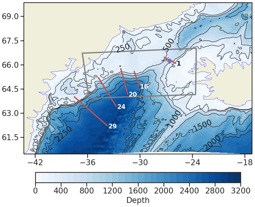
Figure 1 Regional model domain with the ocean depth in colour. The 250, 500, 1000, 1500, and 2000 m depth isobaths are contoured in black. The grey box indicates the region where the two-way grid refinement (1∕36 and $\mathrm{1}/\mathrm{60}{}^{\circ }$) is applied in some simulations. The locations of the various sections used to monitor the model solution are shown by the red lines. Section 1 is the reference section chosen for the sill.

2.2 Initial conditions, surface and open boundary forcing

Data used to initialize the simulation and to drive the flow at the prescribed open boundaries are obtained from an ORCA12 simulation. This global simulation was initialized with temperature and salinity values from a climatology (Levitus, 1998) and started from rest. The atmospheric forcing that was used is the daily mean climatology of the 6-hourly DFS4.4 atmospheric forcing (Brodeau et al., 2010). The forcing data of each day of the year are the climatological mean of that day calculated over the period 1958 to 2001 (see Penduff et al., 2018, for details). This global simulation was run for almost 9 decades with this climatological forcing being repeated every year. It has also been used in the studies of e.g. Sérazin et al. (2015) and Grégorio et al. (2015) to study the intrinsic inter-annual variability. Every DSO model simulation used in the present study (the control run and all sensitivity runs) is initialized with the state of the global run on 1 January of year 72 and is run for a period of 5 years (until year 76). The atmospheric forcing is the same as in the global run and is also repeated every year. The data used at the open boundaries of the DSO domain are extracted from years 72 to 76 of the global simulation (5 d mean outputs), so the open boundary forcing is fully consistent with the atmospheric forcing and the initial state.

We have chosen such a simulation scenario because several decades have passed from the initialization of the global run, and the model has reached a dynamical equilibrium and is close to thermodynamical equilibrium, which results in a negligible drift in the mass field. This allows us to undoubtedly attribute the changes seen in the sensitivity experiments to the changes made in the model setting. During this period the transport at the sill of the Denmark Strait is very stable and close to observed values (∼3 Sv, see Sect. 2.3).

In this scenario, the initial bottom stratification is expected to be particularly affected by biases introduced in the properties of the water masses by the unrealistic representation of the overflows in the z-coordinate framework, so any improvement achieved in the representation of the overflow should be rapidly identified. However, the presence of these model biases reduces the relevance of the comparison to observations.

2.3 Control simulation DSO12.L46

A control simulation (referred to as DSO12.L46) is performed with the characteristics described in Sect. 2.1 and the initial and forcing conditions described above. As expected from its design, the solution of the DSO12.L46 5-year-long control run very faithfully reproduces the solution of years 72 to 76 of the global ORCA12 run. This was verified in different aspects of the circulation. The large-scale circulation patterns are found to be very similar in both simulations, as illustrated with the surface and bottom currents shown in Fig. 2. The predominant currents such as the East Greenland Current (EGC), the Irminger Current (IC), and the DSO itself are very similar between the global and the regional model. This circulation scheme also compares well with that described from observations in Daniault et al. (2016) and from an ORCA12 model circulation simulation in Marzocchi et al. (2015). The correspondence between the global and control runs regarding the properties of abyssal waters was confirmed, especially at 29 different sections along the path of the overflow; the section locations are outlined in Appendix B, as is the correspondence in transport and bottom mean temperature across these sections (not shown). The bottom temperature in the Irminger Basin was found to be very similar in both simulations, with a diluted signature of the overflow waters as expected from a z-level model after a simulation of several decades. Therefore, this regional model appears to be a reliable simulator of what the global model produces in that region.

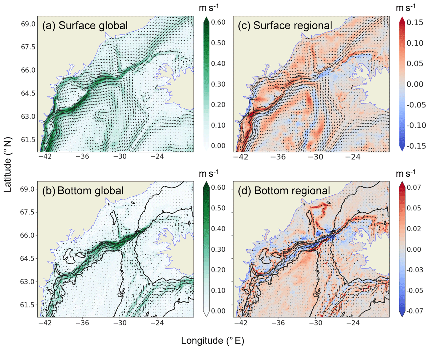
Figure 2 Surface (a) and bottom (b) mean currents (year 76) in the global ORCA12 simulation. Vectors and colours indicate current direction and speed (m s⁻¹). Surface (c) and bottom (d) mean currents (year 76) in the regional DSO12.L46 regional simulation. Vectors indicate the direction of the current. Colours indicate the current speed difference between the global and the regional simulation (m s⁻¹). Blue and red indicate that the current speed is greater or smaller in the global or regional simulation.

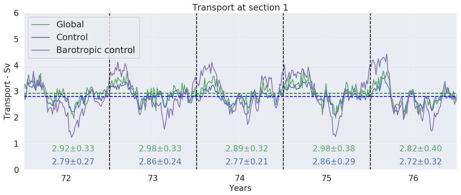
Figure 3 Time evolution of the volume transport of waters of potential density greater than σ₀=27.80 kg m⁻³ at the sill section (section 1 in Fig. 1) in the control (blue line) and the global (green line) simulations (the latter providing the open boundary conditions). Annual mean and SD (Sv) are indicated for every individual year of simulation. The depth-integrated (barotropic) transport is shown for the control simulation (purple line). 5 d mean values were used to produce this figure.

Most important for the present study are the properties of the overflow “source waters”, i.e. the properties of the waters at the sill of the Denmark Strait. Figure 3 shows the volume transport at the sill of waters flowing below the 27.8 isopycnal. Both the global and the control runs show a very similar mean and variability as well as a transport that is very steady during the 5 years of simulation. The model mean (∼3 Sv) is comparable to but in the lower range of the values published in the work of Macrander et al. (2005) and Jochumsen et al. (2012). The standard deviation computed from 5 d outputs (∼0.3 Sv in the control run, increasing to ∼0.7 Sv when calculated from daily values) is rather small when compared to the 1.6 Sv of Macrander et al. (2005). The modelled flow of dense waters presents a marked seasonal cycle which is not present in observations (Jochumsen et al., 2012). This signal is the signature of the large seasonality of the barotropic flow (Fig. 3) that constrains the whole water column.

Figure 4 presents the characteristics of the mean flow across the sill. The model simulation is compared to the data of Mastropole et al. (2017), who processed over 110 shipboard hydrographic sections across the Denmark Strait (representing over 1000 temperature and salinity profiles) to estimate the mean conditions of the flow at the sill. Compared with the compilation of observations by Mastropole et al. (2017) (Fig. 4a) the model simulation (Fig. 4b) shows a consistent distribution of the isopycnals. However, the observations exhibit waters denser than 28.0 in the deepest part of the sill, which the model does not reproduce. Large flaws are noticed regarding the temperatures of the deepest waters, which are barely below 1 ^∘C when observations clearly show temperatures below 0 ^∘C (also seen in the observations presented in e.g. Jochumsen et al., 2012, 2015; Zhurbas et al., 2016). A bias toward greater salinity values (not shown) is also found in the control experiment, which shows a bottom salinity of 34.91 compared to 34.9 in the observations shown in Mastropole et al. (2017), but the resulting stratification in density shows patterns that are consistent with observations. The distribution of velocities (Fig. 4c) is also found to be realistic when compared with observations (i.e. Fig. 2b of Jochumsen et al., 2012), with a bottom-intensified flow of dense waters (up to 0.4 m s⁻¹) in the deepest part of the sill. Although the present set-up is designed to investigate model sensitivity in twin experiments and not for comparison with observational ends, the control run appears to provide a flow of dense waters at the sill that is stable over the 5-year period of integration and qualitatively reproduces the major patterns of the overflow source waters seen in the observations. Therefore, despite existing biases, the presence of a well-identified dense overflow at the sill confirms the adequacy of the configuration for the sensitivity studies.

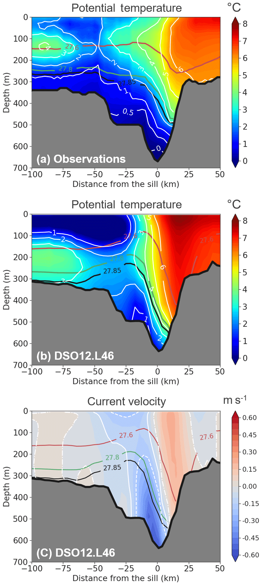
Figure 4 Mean flow characteristics (annual mean of year 76) in the global simulation for a section across the sill. Temperature (^∘C) is represented by colours and white contours for (a) the observations (Mastropole et al., 2017) and (b) the control simulation (DSO12L46 $\mathrm{1}/\mathrm{12}{}^{\circ }$ and 46 vertical levels). Potential density values (σ₀) are shown by the contour lines coloured in red (27.6), green (27.8), and black (27.85). (c) The velocity normal to the section in the control simulation (with southward velocity in blue being negative). White lines indicate the 0 m s⁻¹ contour (dashed–dotted line), the −0.1 m s⁻¹ contour (full line), and the −0.2 m s⁻¹ contour (dashed line).

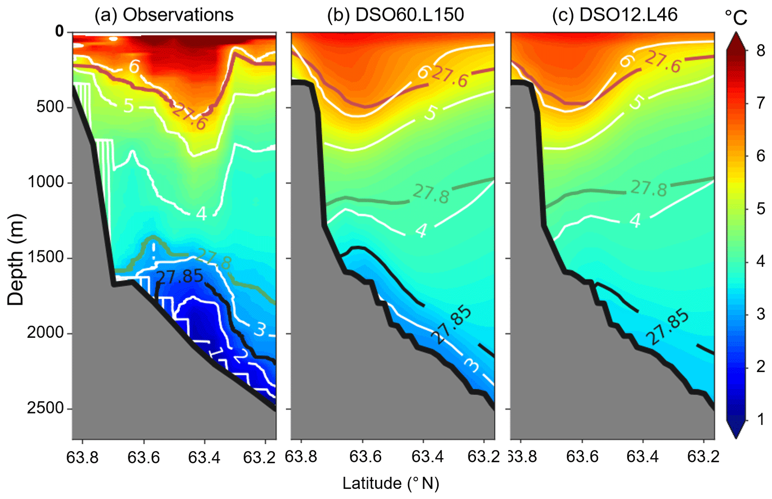
Figure 5 Potential temperature (^∘C) at section 29 in (a) the observations (ASOF6 section; Quadfasel, 2010), (b) the $\mathrm{1}/\mathrm{60}{}^{\circ }$, 150-level simulation (annual mean), and (c) the $\mathrm{1}/\mathrm{12}{}^{\circ }$, 46-level simulation (annual mean). Red, green, and black full lines are isopycnals 27.6, 27.8, and 27.85. White lines are isotherms in 1^∘C intervals. In panel (b), section 29 is outside (100 km downstream) the $\mathrm{1}/\mathrm{60}{}^{\circ }$ AGRIF zoom, so the effective resolution is $\mathrm{1}/\mathrm{12}{}^{\circ }$, but the water masses acquired their properties upstream within the $\mathrm{1}/\mathrm{60}{}^{\circ }$ resolution zoom.

Finally, in order to assess improvements in the sensitivity tests, the major flaws of the control simulation must be described. If similarities with observations are found at the sill, the evolution of the DSO plume in the Irminger Basin is shown to be unrealistic in the present set-up of the control simulation and presents the same flaws as in the global run. This is demonstrated by the analysis of the temperature and potential density profiles at the most downstream cross section (section 29), wherein the model solution is compared to observations (Fig. 5), and at the other cross sections along the path of the DSO in the control simulation (Figs. 6a, c and 7a, c). The evolution of the DSO plume as it flows southward along the East Greenland shelf break is represented by a well-marked bottom boundary current (e.g. the bottom currents in Fig. 2) carrying waters of greater density than the ambient waters. Far downstream of the sill (section 29), the observations show a well-defined plume of cold water confined below the 27.8 isopycnal under 1500 m of depth (Fig.  5a). The bottom temperature is still below 1 ^∘C. In the control simulation (Fig. 5c), one can clearly identify the core of the DSO plume by the 27.85 isopycnal, so it is clear that the plume has been sinking to greater depth as it moved southward. This evolution is only qualitatively consistent with the observations at this section. The modelled plume is significantly warmer and exhibits a core temperature of 3.5^∘ (against 2 ^∘C or less in the observations). The plume is also much wider than observed and exhibits much smaller temperature and salinity gradients separating the plume from the interior ocean, indicating a greater dilution with ambient waters. The plume is barely distinguishable from the ambient fluid below 2000 m, while it is still well-marked at that depth in the observations. The sinking and dilution of the plume as it flows southward along the slope of the Greenland shelf are well-illustrated in Figs. 6 and 7 (panels a and c), which display the potential temperature at the other sections. If the overflow waters are still well-marked at section 16 (Fig. 6a), they are barely distinguishable from the ambient water at section 29.

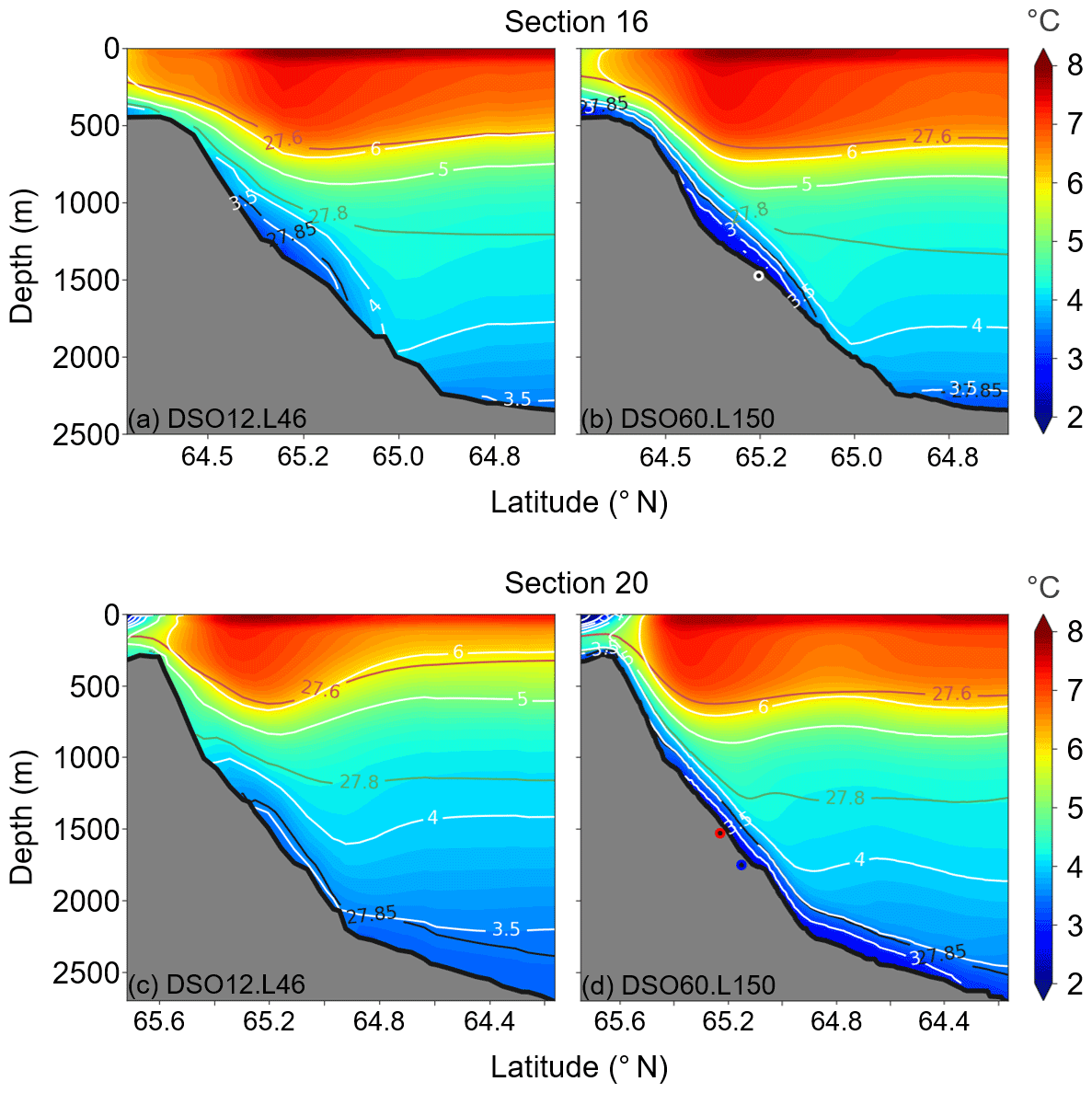
Figure 6 Distribution with depth of the annual mean temperature (fifth year of model run) at section 16 (Dohrn Bank array) for (a) simulation DSO12.L46 and (b) simulation DSO60.L150 (in the refined grid), as well as at section 20 (Spill Jet section) for (c) simulation DSO12.L46 and (d) simulation DSO60.L150 (in the refined grid). Temperature (^∘C) is represented by colours with white contours. Potential density values (σ₀) are shown by the contour lines coloured in red (27.6), green (27.8), and black (27.85). The white-rimmed dot in (b) corresponds to the location of the profiles displayed in Fig. 15, and the red-rimmed and blue-rimmed dots in (d) correspond to the locations of the profiles displayed in Fig. 13.

Figure 7 As in Fig. 6 at section 24 (TTO array) for (a) simulation DSO12.L46 and (b) simulation DSO60.L150, as well as at section 29 (Angmagssalik array) for (c) simulation DSO12.L46 and (d) simulation DSO60.L150.

The bottom temperature shown in Fig. 8a illustrates this excessive dilution of the overflow waters. Indeed, the cold water tongue seen at the bottom of the Denmark Strait at a temperature of about 2 ^∘C clearly sinks as it extends to the southwest and crosses the 1000 and 1500 m isobaths. But as it sinks, it is rapidly diluted, loses its “cold water” character, and is not distinguishable from the background waters beyond 64.5^∘ N. Such a plot of the bottom temperature summarizes rather well what we also learned in the analysis of the cross sections (e.g. Fig. 5). The same plot for the salinity (not shown) shows waters fresher than surrounding waters in the overflow path, with a salinity that increases from 34.91 at the sill to around 34.96 at 1000 m and reaches the background value (∼ 35.02) at 1500 m of depth. This demonstrates the large dilution by entrainment with the waters of the Irminger Current in the final solution.

3 Results from sensitivity experiments

We performed a large set of simulations (over 50) with different settings of the DSO model configuration in order to better understand the impact of the different parameters on the final representation of the DSO at a resolution of $\mathrm{1}/\mathrm{12}{}^{\circ }$, including a few with local grid refinement. The detailed list of these experiments is provided in Appendix A. Following the convention for DSO12.L46, the simulations are referred to as DSOxx.Lyy; xx provides information on the horizontal grid resolution (e.g. 36 for $\mathrm{1}/\mathrm{36}{}^{\circ }$) and yy on the number of vertical levels (e.g. 150 for 150 levels). After testing different physical parameterizations, numerical schemes, and grid resolutions, we concluded that the only parameters affecting the overall representation of the overflow in a significant way are the horizontal and vertical resolutions. No significant impact was found on the representation of the DSO for all the other parameters tested, with the flaws described in the previous section resisting the changes. Therefore, we only present the results obtained when the resolution (vertical, horizontal, or both) is changed. The other sets of sensitivity tests are very briefly discussed in Appendix A.

From the large set of diagnostics performed to assess the impact of model changes on the DSO, it was found that the analysis of the bottom temperature in the Irminger Basin is quite a pertinent way to provide a first assessment of the changes in the properties of the overflow. This diagnostic is consequently used to first compare the different sensitivity simulations, and additional diagnostics are used later for more quantitative assessments of the DSO representation. Improvements between sensitivity tests are identified when one or several of the major flaws described in the previous (Sect. 2.3) section are reduced. These major flaws, identified on the time mean properties of the overflow of the control simulation (Sect. 2.3) are the following: a bottom temperature that is too warm; an overflow not deep enough; and weak temperature gradients between the plume and the ambient fluid (a dense water plume that is not well-defined, indicating too much dilution.)

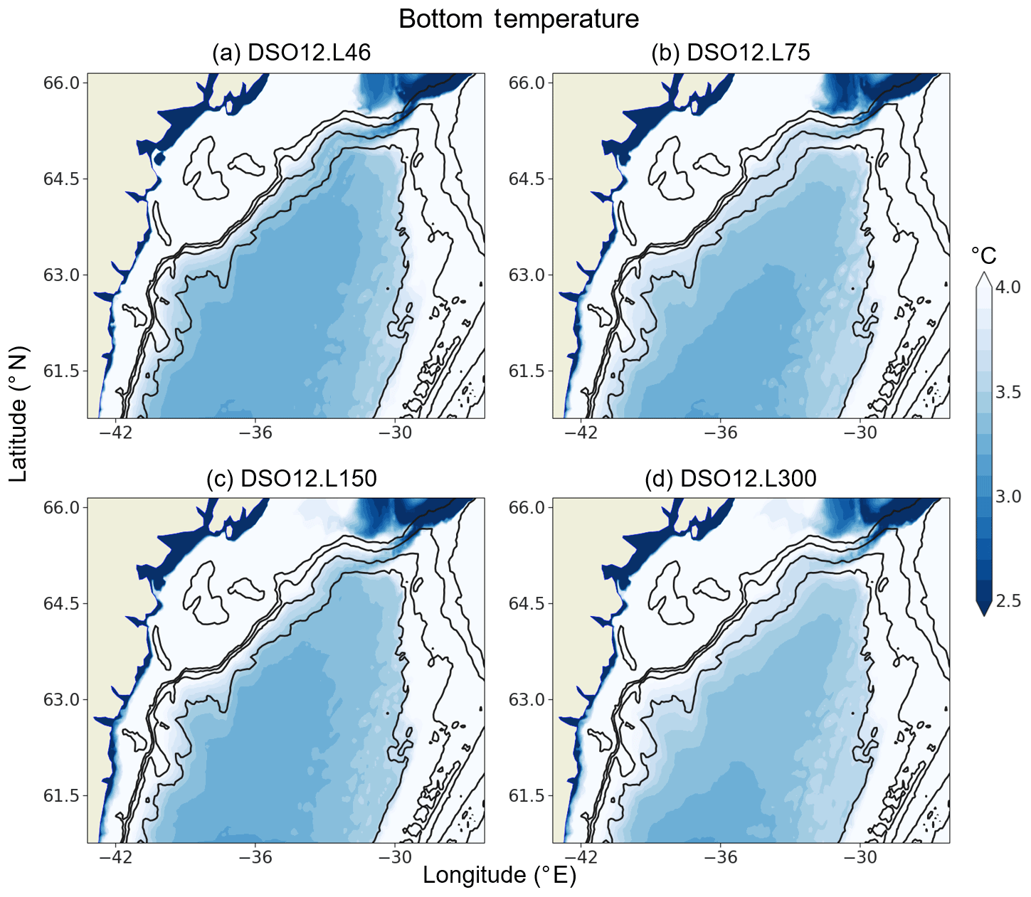
Figure 8 Annual mean bottom temperature (fifth year of simulation; ^∘C) at $\mathrm{1}/\mathrm{12}{}^{\circ }$ horizontal resolution in simulations with differing numbers of vertical levels: (a) 46 levels (DSO12.L46), (b) 75 levels (DSO12.L75), (c) 150 levels (DSO12.L150), and (d) 300 levels (DSO12.L300). Isobaths 500, 1000, 1500, and 2000 m are contoured in black.

3.1 Sensitivity to vertical resolution at $\mathrm{1}/\mathrm{12}{}^{\circ }$

The first set of tests that we present is for the sensitivity of the DSO representation to the vertical resolution at $\mathrm{1}/\mathrm{12}{}^{\circ }$ horizontal grid resolution. The DSO12.L46 control run (46 levels) is compared with simulations with 75, 150, and 300 vertical levels, with all other parameters being identical. The mean bottom temperature of the fifth year of these four simulations (Fig. 8) reveals that the increase in vertical resolution at $\mathrm{1}/\mathrm{12}{}^{\circ }$ works to the detriment of the representation of the overflow. In the 75-level case, the descent of the DSO plume stops at the 1500 m isobath, blocked by a westward flow of warm Irminger waters that invades the 1500 to 2000 m depth range. This yields a general warming of the bottom waters in the Irminger Basin and along the whole East Greenland shelf break. The overflow representation improves slightly in the 150-level case as the DSO plume still reaches the 2000 m isobath, feeding the deep basin, but with less efficiency than in the 46-level case. Finally, the representation of the DSO is even more degraded in the 300-level case, with this resolution exhibiting the greatest dilution of the DSO waters among all resolutions. This deterioration of the overflow properties was verified in all the other diagnostics (hydrographic sections, T–S diagrams, etc.).

To understand that behaviour, one recalls how the cascading of dense water is treated in the z-coordinate NEMO framework. In the case of static instability (i.e. when the fluid at a given level has a greater potential density than the fluid at the next level below), the vertical mixing coefficient, usually calculated with the TKE closure scheme, is assigned a very large value (usually 10 m² s⁻¹). This instantaneously (i.e. over one time step) mixes the properties (temperature, salinity, and optionally momentum) of the two cells, re-establishing the static stability of the stratification. This parameterization, referred to as EVD (enhanced vertical diffusion, already described in Sect. 2.1), is at work to simulate the sinking (convection) and the cascading (overflow) of dense waters. Note that when the EVD was not used in our experiments, we noticed that the TKE mixing scheme often produced values of the diffusion coefficient larger than 1 m² s⁻¹ and in very particular cases exceeding 10 m² s⁻¹.

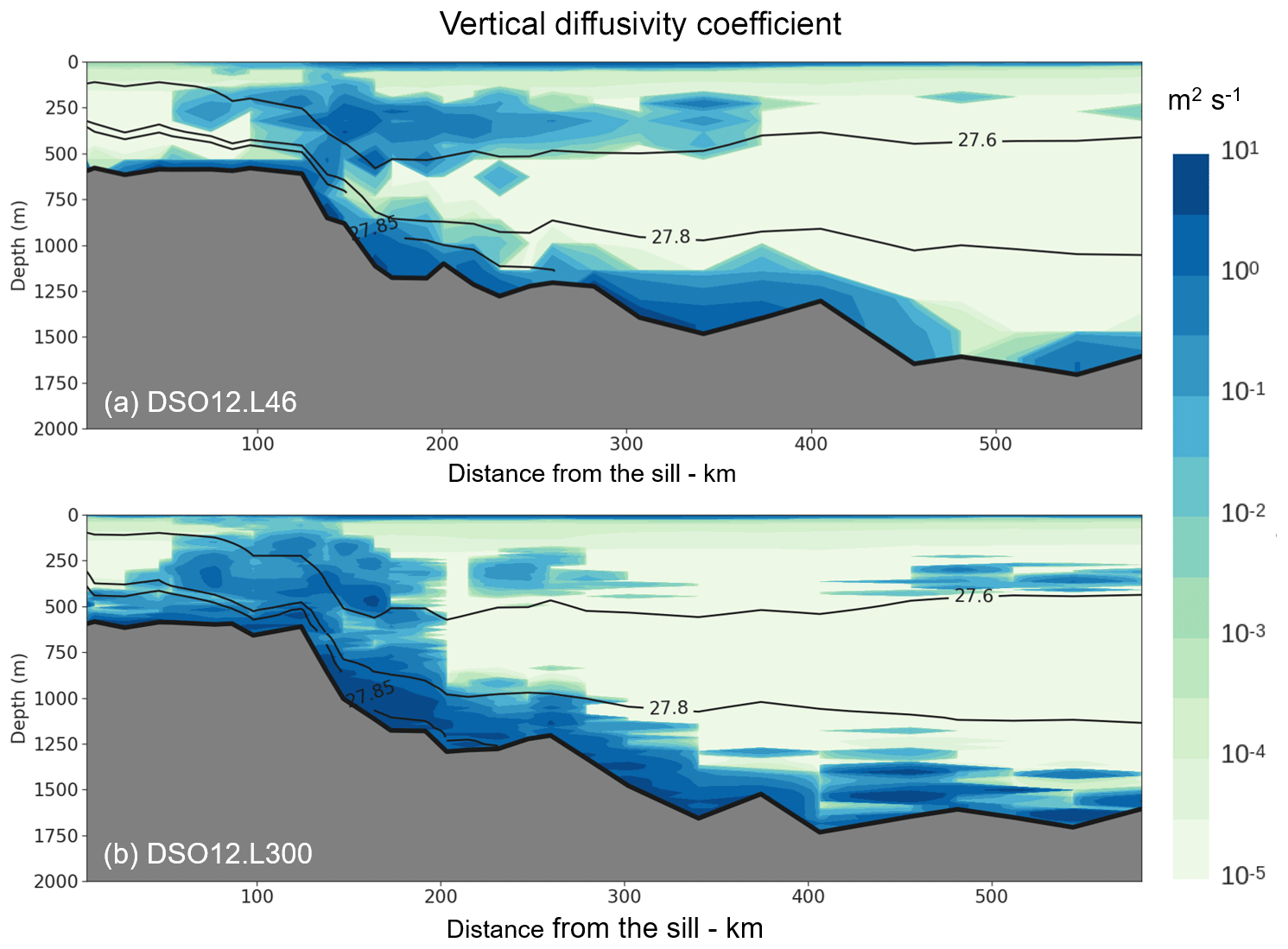
Figure 9 Vertical diffusivity coefficient (K_z, summer mean in the fifth year of simulation) along the path of the vein calculated for (a) simulation DSO12.L46 and (b) simulation DSO12.L300. Potential density values (σ₀) are shown by the contour lines.

The vertical diffusivity along the path of the overflow is shown in Fig. 9 for the 46- and the 300-level cases (the definition and method of calculation of the overflow path are given in Appendix B). Compared to the 46-level case (Fig. 9a), the 300-level case (Fig. 9b) exhibits greater values of the diffusion coefficient near and above the bottom along the path of the overflow. This enhanced mixing affects the overflow plume, which 200 km after the sill does not contain waters denser than 27.85, while such waters are still found 300 km down the sill in the 46-level case. The 300-level case also exhibits large values of the diffusion coefficient at intermediate depth (between isopycnals 27.8 and 27.6). This is driven by the vertical shear existing between the northward surface current passing through the Denmark Strait (the NIIC), which is very variable in position and intensity, and the southward deep current carrying the overflow waters (e.g. Spall et al., 2019). We notice that the mixing is significantly greater in the high-resolution case, which indicates that this process could also contribute to the dilution of the overflow plume. However, it does not seem to affect the thickness of the 27.8 isopycnal. An explanation for this is searched for following the paradigm of Winton et al. (1998), which states that the horizontal and vertical resolutions should not be chosen independently: the slope of the grid (Δz∕Δx) has to equal the slope of the topography (α) to produce a proper descent of the dense fluid (see their Fig. 7). If this is not the case, the vein of dense fluid thickens by mixing with the ambient fluid at a rate proportional to the ratio of the slopes $\mathit{\alpha }/(\mathrm{\Delta }z/\mathrm{\Delta }x)$.

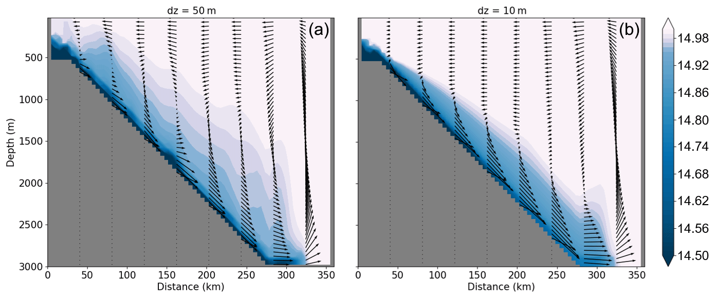
Figure 10 Idealized experiment simulating the rationale explored in Fig. 7 of Winton et al. (1998). Cold water (10 ^∘C) descends a shelf break in a configuration with ambient water at 15 ^∘C after 9 d of simulation. Two vertical resolutions are used: (a) Δz=50 m, (b) Δz=10 m. Temperature (^∘C) is represented by colours. Vectors represent the velocity, with the vertical velocity being re-scaled according to the grid aspect ratio in the case in panel (a).

To show how NEMO follows this concept, we simulate the descent of a continuous source of cold water down a shelf break in an idealized configuration (with no rotation). The configuration (Fig. 10) is as follows. A 20 km wide shelf of depth 500 m is located on the left side of the 2D domain. It is adjacent to a shelf break 250 km wide reaching the depth of 3000 m, and then the bottom is flat. Initial conditions are as follows: a blob of cold water is placed on the bottom of the shelf with a temperature of 10 ^∘C, with the temperature of the ambient fluid in the rest of the domain being 15 ^∘C and the salinity being constant (35) in the whole domain. During the simulation, the temperature is restored on the shelf to its initial value to maintain the source of cold water. A relaxation to the ambient temperature is applied over the whole water column in the last 50 km of the right side of the domain in order to evacuate the cold water. The horizontal grid resolution is 5 km (comparable to the $\mathrm{1}/\mathrm{12}{}^{\circ }$ resolution of our regional DSO configuration). Two simulations with different vertical resolutions are run. The first one uses 60 levels of equal thickness (50 m) such that the local grid slope always equals the slope of the bathymetry (Fig. 10a; Δz=50 m). In the second simulation, the vertical resolution is increased by a factor of 5 (300 vertical levels; Fig. 10b; Δz=10 m). In the absence of rotation, the pressure force pushes the blob over the shelf break and the EVD mixing scheme propagates the cold water down to the bottom as the blob moves toward deeper waters, generating an overflow plume. After about 5 d, the front of the plume has reached the end of the shelf break and entered the damping zone at the right side of the domain, reaching a quasi-stationary regime. In that regime, the overflow simulated in the 300 vertical levels run (i.e. with a local grid slope smaller than the topographic slope) presents warmer bottom waters (Fig. 10b) than in the 60-level run, in agreement with the results obtained with the realistic DSO12 configuration. Note that the vertical shear is more confined in the high-resolution case, which prevents the upward extent of the TKE-induced mixing of the upper part of the overflow that is seen in the low-resolution case. Note that when using a realistic bottom topography, the topographic slope will present large local variations and that it will be almost impossible to match the two slopes over the whole domain in a z-coordinate context. Therefore, increasing the number of vertical levels will not systematically degrade the overflow representation everywhere.

A set of simulations tested the effect of the different closure (i.e. vertical mixing) schemes available in NEMO (TKE with and without EVD; k−ϵ with and without EVD, constant diffusivity + EVD, Madec et al., 2016). It was found that the choice of the vertical mixing scheme has a very small (insignificant) impact on the final representation of the overflow at $\mathrm{1}/\mathrm{12}{}^{\circ }$.

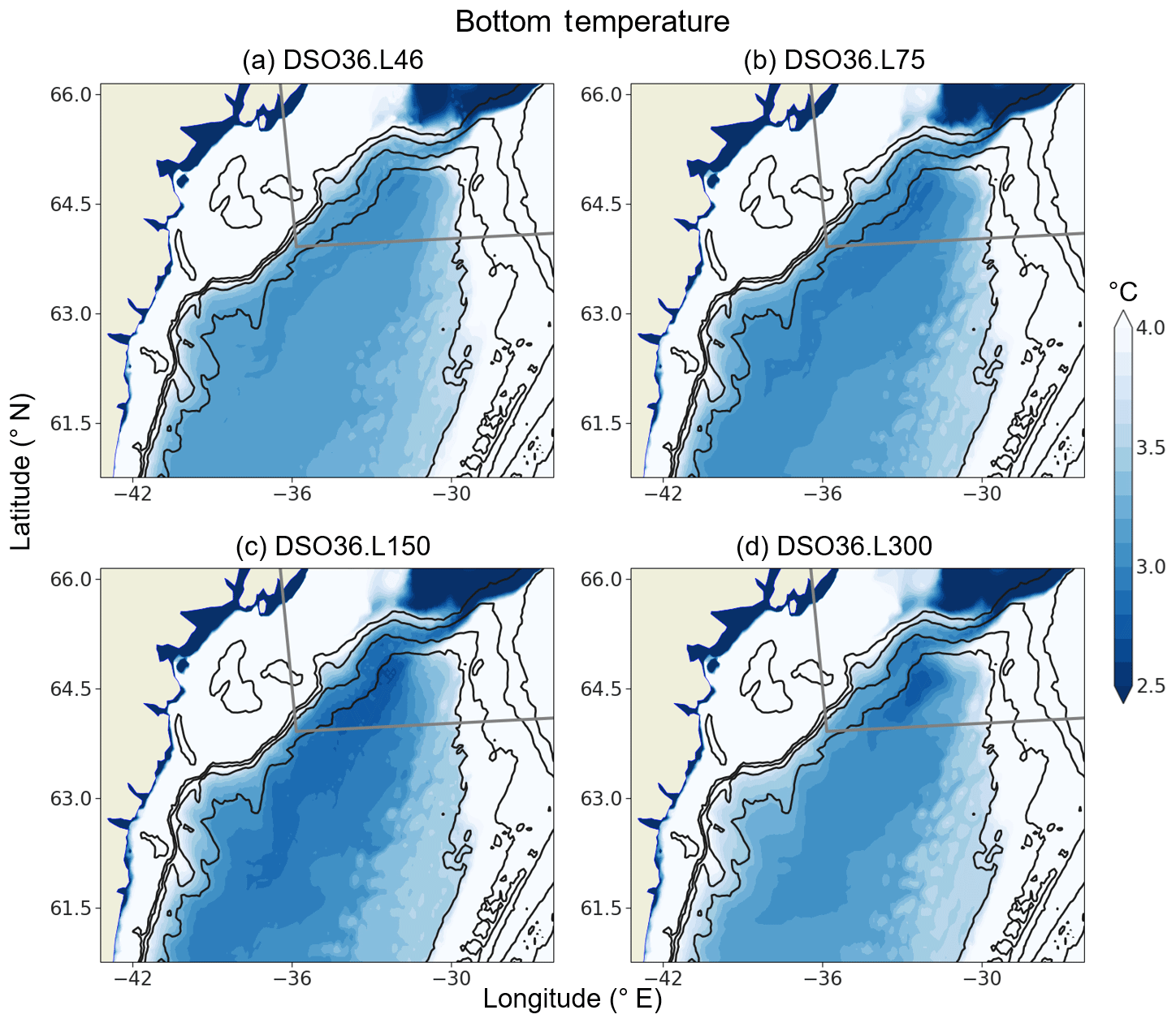
Figure 11 Annual mean of the bottom temperature of year 5 of simulations using grid refinement ($\mathrm{1}/\mathrm{36}{}^{\circ }$): (a) DSO36.L46, (b) DSO36.L75, (c) DSO36.L150, (d) DSO36.L300. Isobaths 500, 1000, 1500, and 2000 m are contoured in black.

3.2 Sensitivity to a local increase in horizontal resolution

3.2.1 The $\mathrm{1}/\mathrm{36}{}^{\circ }$ case

The second set of tests that we present is for the sensitivity of the DSO representation to the vertical resolution using a local horizontal refinement of $\mathrm{1}/\mathrm{36}{}^{\circ }$ in the overflow region (see Fig. 1). The same range of vertical levels as for the $\mathrm{1}/\mathrm{12}{}^{\circ }$ resolution case is investigated: 46 levels (DSO36.L46), 75 levels (DSO36.L75), 150 levels (DSO36.L150), and 300 levels (DSO36.L300). The annual mean bottom temperature of the fifth year of simulation is shown in Fig. 11. Compared to the $\mathrm{1}/\mathrm{12}{}^{\circ }$ cases, the $\mathrm{1}/\mathrm{36}{}^{\circ }$ cases present, at an equivalent number of vertical levels, significantly colder bottom temperatures in the Irminger Basin and along the East Greenland shelf break. This amelioration is rather small at 46 levels (Fig. 11a; the cooling is ∼ 0.4 ^∘C) but is more significant for the other vertical resolutions. The greatest improvement is observed when the number of vertical levels is increased to 150 levels (Fig. 11c). In this case the signature of the DSO becomes evident. The bottom temperature of the overflow plume in its first 100 km cooled from a value of ∼ 3.6 ^∘C at $\mathrm{1}/\mathrm{12}{}^{\circ }$ (Fig. 8a) to a value of ∼ 2.7 ^∘C (a remarkable cooling of ∼ 0.9 ^∘C), while the temperature at the sill did not change.

The situation changes when increasing to 300 levels (Fig. 11d). The tendency for improvement noticed when increasing from 46 to 150 levels reverses, and the representation of the overflow is slightly degraded. This result is coherent with the explanation given for the $\mathrm{1}/\mathrm{12}{}^{\circ }$ case. Once a vertical resolution adequate for a specific horizontal resolution is set for a given slope, an increase in the vertical resolution will deteriorate the DSO representation by introducing excessive vertical mixing. A relevant remark here is that over-resolving the slope vertically worsens the overflow representation, which is consistent with the conclusions of Winton et al. (1998). In other words, there is an optimal number of vertical levels to be used for a given horizontal resolution for a given slope. Given the large variety of slopes present in the oceanic topography (and encountered by an overflow during its descent), modelling topographically constrained flows with z coordinates appears to be a quite difficult task.

3.2.2 The $\mathrm{1}/\mathrm{60}{}^{\circ }$ case

We now evaluate the representation of the DSO at $\mathrm{1}/\mathrm{60}{}^{\circ }$ (using a local refinement in the area shown in Fig. 1) with 46, 75, 150, and 300 vertical levels. At this resolution, the 46-level and 75-level cases show a solution very similar to that presented at the resolution of $\mathrm{1}/\mathrm{36}{}^{\circ }$ (no significant additional improvement, no figure shown). A significant change is again observed for 150 levels (Fig. 12a). The signature of the overflow waters at the bottom is even stronger in this case, with the cooling of the overflow plume being ∼ 1.1 ^∘C when compared to the $\mathrm{1}/\mathrm{12}{}^{\circ }$ solution (Fig. 8a) and ∼ 0.2 ^∘C compared to the $\mathrm{1}/\mathrm{36}{}^{\circ }$ case.

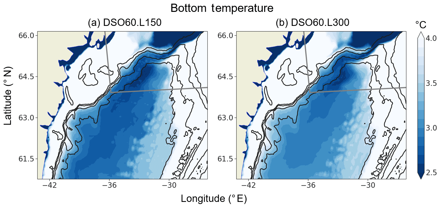
Figure 12 Annual mean of the bottom temperature in the fifth year of simulations using a grid refinement of $\mathrm{1}/\mathrm{60}{}^{\circ }$ for (a) 150 vertical levels (DSO60.L150) and (b) 300 vertical levels (DSO60.L300). Isobaths 500, 1000, 1500, and 2000 m are contoured in black. The grey box indicates the area of refinement.

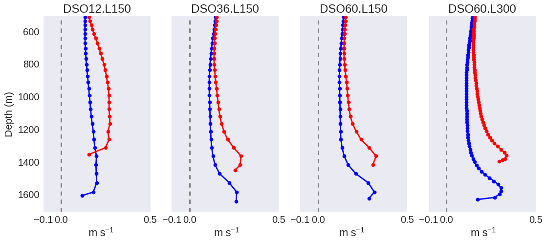
Figure 13 Vertical profiles (annual mean) of the quasi-along-slope velocity (i.e. velocity normal to the section) at the two locations of section 20 indicated in Fig. 6d for simulations (a) DSO12.L150, (b) DSO36.L150, (c) DSO60.L150, and (d) DSO60.L300.

The solution of the 300-level case at $\mathrm{1}/\mathrm{60}{}^{\circ }$ (Fig. 12b) represents an improvement compared to the $\mathrm{1}/\mathrm{36}{}^{\circ }$ case with the same vertical resolution. However, compared to the $\mathrm{1}/\mathrm{60}{}^{\circ }$ and 150-level solution (Fig. 12a), it shows a slightly greater dilution of the overflow and warmer temperatures at the bottom. Also, the propagation of the dense water away from the refinement area is clearly better with 150 levels. This should be taken into consideration when choosing the refinement region if used in global implementations. Improvements brought to the representation of the overflow by the resolution increase to $\mathrm{1}/\mathrm{60}{}^{\circ }$ and 150 levels can also be seen in Figs. 6 and 7, and they are quantitatively assessed in the following section (Sect. 4). At every section, the DSO60.L150 overflow (panel b and d) is clearly identified by a vein of cold waters well-confined along the slope with temperatures below 3 ^∘C and always at least 0.5 ^∘C colder than in the reference simulation (DSO12.L46; panels a and c). Temperature gradients between the core of the overflow and the interior ocean are also significantly increased, and the isopycnal 27.85 marks the limit of the vein of fluid very well. If a warm bias still exists compared to the observations of Quadfasel (2010) (bias in part due to the unrealistic properties of the interior entrained waters), the agreement of the overflow pattern with the observations is nevertheless greatly improved.

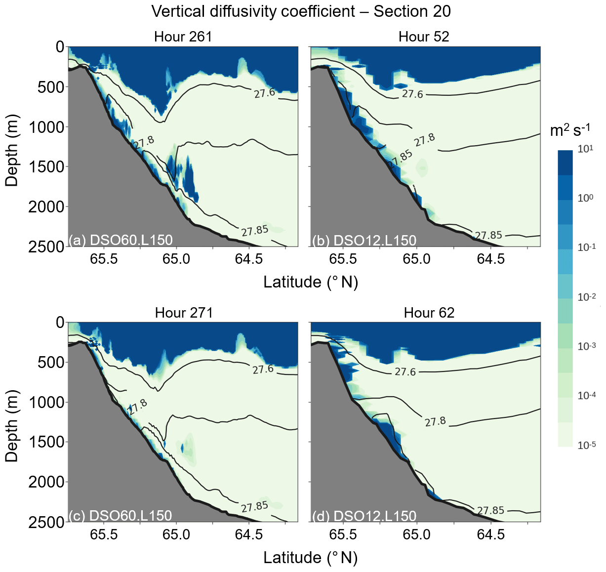
Figure 14 Vertical diffusivity coefficient (K_z, hourly mean) at section 20 in simulations (a, c) DSO60.L150 (in the refined grid) and (b, d) DSO12.L150 in wintertime (with a 10 h difference). In black: contours of isopycnals 27.6, 27.80, and 27.85.

4 Eddy-resolving solution ($\mathrm{1}/\mathrm{60}{}^{\circ }$ grid and 150 levels)

The worsening of the DSO representation with increasing vertical resolution until a certain extent is observed with the three horizontal resolutions used in this study (1∕12, 1∕36, and $\mathrm{1}/\mathrm{60}{}^{\circ }$). The analysis of the high vertical diffusivity values due to the EVD demonstrated the dominant impact of this parameterization on the overflow at the resolution of $\mathrm{1}/\mathrm{12}{}^{\circ }$ and emphasized the need for coherent vertical and horizontal grids. However, the improvements observed in both the DSO36.L150 and DSO60.L150 cases suggest that this impact is reduced and other drivers take control of the evolution of the overflow plume when higher horizontal grid resolutions are used. To reach a better understanding of the reasons for improvement, we perform in this section an analysis of the overflow structure in the $\mathrm{1}/\mathrm{60}{}^{\circ }$ and 150-level simulation (DSO60.L150).

Figure 13 shows vertical profiles of the mean along-slope velocity at two different locations on the shelf break at section 20 from four different simulations which use a large number of vertical levels (150 or 300). All profiles, except that of $\mathrm{1}/\mathrm{12}{}^{\circ }$ with the 150-level case, show a bottom-intensified boundary current confined in the first 200 m above the bottom and the presence of a sheared bottom Ekman layer better resolved with 300 levels but still well-marked with 150 levels. This indicates the presence of a well-defined overflow plume, as shown for DSO60.L150 in Fig. 6d. This bottom signature has already been described in observations (Paka et al., 2013). In the other $\mathrm{1}/\mathrm{60}{}^{\circ }$ cases with lower vertical resolution (DSO60.L46 and DSO60.L75, not shown), the Ekman-driven vertical shear cannot be resolved and the dynamics of the current are dominated by the EVD mixing.

The absence of this bottom-confined intensified current in the DSO12.L150 simulation can be related to a similar cause, although the vertical resolution is sufficient to partially resolve the Ekman bottom layer. The analysis of the vertical mixing coefficient (Fig. 14b, d) shows a very intense mixing in a rather thick layer all along the slope (between 500 and 2200 m), and, according to the previous rationale, the reason is the convective adjustment (EVD) governing the near-bottom physics. This enhanced mixing seriously limits the development of a sheared flow in the bottom layer.

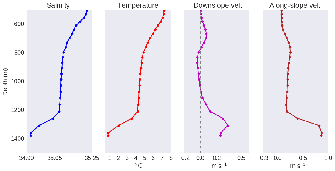
Figure 15 Vertical profiles of the physical properties of the overflow plume in simulation DSO60.L150 (hour 10 on 1 February of year 5) at section 16 for the location indicated with a white-rimmed dot in Fig. 6b. (a) Salinity, (b) temperature, (c) cross-slope velocity, and (d) along-slope velocity.

In the case of DSO60.L150 (Fig. 14a, c) a small but noticeable mixing remains confined to a very thin bottom layer below the 27.85 isopycnal, and very little mixing occurs in the core of the overflow plume. Intermittent static instabilities occur between the 27.85 and the 27.8 isopycnals (shown by the large values of K_z in Fig. 14a). Our analysis (no figure shown) indicates that these instabilities are generated by advection toward the deep ocean of bolus of dense water by a cyclonic bottom-intensified eddy. After the eddy passed through the section (Fig. 14c) the stratification was again stable. Such features are not seen in the $\mathrm{1}/\mathrm{12}{}^{\circ }$ simulation (Fig. 14b, d) because the horizontal resolution does not properly resolve the mesoscale eddies. This behaviour is consistent with the physical processes present in the DSO, the simultaneous action of the shear governing the entrainment in the overflow plume and the density gradient driving the overflow to the bottom. In this way, the use of coherent horizontal and vertical resolutions plays a key role since it allows the convective adjustment to occur in a limited portion of the plume without interfering with the other important processes driving the physics in the vein of dense fluid. We identify three conditions for a proper representation of the DSO: coherent vertical and horizontal grids to avoid excessive convective adjustment (due to EVD or any other scheme); proper vertical resolution to resolve the shear induced by the Ekman layer dynamics; and enough horizontal resolution to resolve the boluses of the DSO (described afterwards). This agrees with what is stated in the idealized study of Laanaia et al. (2010): it is not the increase in vertical viscosity that enables the downslope movement but the resolution of the bottom Ekman layer dynamics.

Continuing with the description of the bottom flow, we show in Fig. 15 the vertical profiles of physical properties at a specific point at section 16, chosen close to where Paka et al. (2013) performed microstructure measurements (65.20^∘ N, 30.41^∘ W) in order to allow for a direct comparison. Our DSO60.L150 simulation reproduces with a high degree of realism the main features of the observed plume (as shown in Fig. 4 of Paka et al., 2013). As in the observations, the plume is nearly 200 m thick and is located between 1200 and 1400 m of depth. Compared to the water above it, the modelled plume is characterized by a freshening of ∼ 0.15 (∼ 0.10 in the observations) and a cooling of 3.0 ^∘C (∼ 3.5^∘C in the observations). The cross-slope and along-slope velocities show a speed-up of the flow in the plume of ∼ 0.2 and ∼ 0.6 m s⁻¹, respectively, in observations, with the corresponding values in the model being 0.3 and 0.7 m s⁻¹. Since this 200 m thick plume is represented by five to six points in the vertical, the use of 150 L might be a lower bound for the number of vertical levels to use in order to properly represent the DSO.

Figure 16 Hourly snapshots of bottom temperature in simulation DSO60.L150 for (a) 4 January at time t0=14 h, (b) time $t=t\mathrm{0}+\mathrm{15}$ h, (c) time $t=t\mathrm{0}+\mathrm{26}$ h, and (d) time $t=t\mathrm{0}+\mathrm{39}$ h. The 500, 1000, 1500, and 2000 m isobaths are contoured.

The boluses of cold waters mentioned in different observational and modelling papers (see, for example, Girton and Standford, 2003; Jochumsen et al., 2015; Magaldi and Haine, 2015; Koszalka et al., 2017) are also reproduced by the model. To illustrate this we show in Fig. 16 the hourly outputs of the bottom temperature in a sequence that lasts only ∼ 40 h. First, in Fig. 16a the DSO appears as a cold water (∼ 1 ^∘C) plume that has already started its descent and is confined between the 500 m and 1000 m isobaths. Boluses of cold water (∼ 2 ^∘C) are also seen a few tens of kilometres downstream in the depth range 1500 to 2000 m and in the deep Irminger Basin. A total of 15 h later (Fig. 16b), the DSO plume has sunk to 1500 m, seems to be adjusted to geostrophy, and flows along isobaths. Another plume of cold water is moving through the sill. In the following 24 h, the first plume moves along the shelf break (Fig. 16c) and breaks into a bolus which brings cold waters to the depth of 2000 m (Fig. 16d). A significant entrainment of surrounding waters occurred during the breaking as the water in the bolus gained about 0.5 ^∘C. The bolus will continue its way to the Angmagssalik array, i.e. section 29 in Fig. 1, and will contribute to cooling the deep Irminger Basin. The second plume has crossed the sill and reached the 1000 m isobath. It will later generate another bolus following the same process. The formation of the bolus happened in only 40 h, showing the high-frequency variability of the overflow and illustrating the difficulty of diagnosing its time mean properties.

We attempted a quantitative comparison with the relatively long-term observations made at the mooring arrays reported in the study of Jochumsen et al. (2015). These arrays correspond to the Sill array (section 1 in Fig. 1), the Dohrn Bank array (section 16 in Fig. 1), and the Angmagssalik array (section 29 in Fig. 1). Following Jochumsen et al. (2015) we reported in (Fig. 17) the minimum time mean bottom temperature at these four sections for certain simulations. This figure summarizes our main findings. In the $\mathrm{1}/\mathrm{12}{}^{\circ }$ simulations, the temperature at the mooring arrays (i.e. the dilution of the overflow) increases with increasing vertical resolution, with DSO12.L46 showing a lesser dilution for the first 200 km of the overflow path than DSO12.L150. The best-performing simulation at $\mathrm{1}/\mathrm{36}{}^{\circ }$ is that with 150 levels (DSO36.L150). It shows a cooling of the bottom waters after the sill of about 0.5 ^∘C when compared to DSO12.L46. At $\mathrm{1}/\mathrm{60}{}^{\circ }$ resolution, the best-performing simulation is also that with 150 levels (DSO60.L150). When compared to the best $\mathrm{1}/\mathrm{12}{}^{\circ }$ simulation (DSO12.L46) it shows an even greater cooling of the bottom waters after the sill (0.7 ^∘C). Increasing the vertical resolution to 300 levels produces a slightly greater dilution of the plume that could be considered insignificant, but the computational cost is doubled. When comparing this set of best-performing simulations with observations, it appears that the model always produces a much greater dilution of the physical properties of the overflow in the first 200 km of its path. Improved initial and boundary conditions (i.e. correcting for the warm bias of 0.3 ^∘C at the sill and for the warm and salty bias of the entrained waters of the Irminger Current) should reduce this difference but to a point which is difficult to estimate. Either way, the 1.5 ^∘C difference shown in Fig. 17 is quite a wide gap that such bias correction will likely not be sufficient to fill.

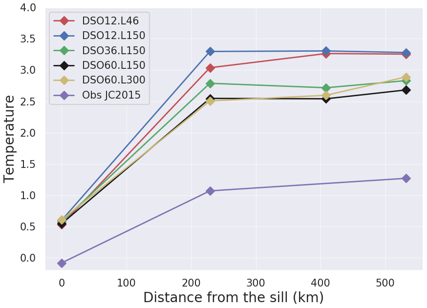
Figure 17 Time mean minimum bottom temperature for five sensitivity simulations at the location of the observational arrays. The results of Jochumsen et al. (2015) are reported as Obs JC2015.

Finally, we would like to point out that the increase in resolution may also improve the representation of topography, despite the fact that it is linearly interpolated from $\mathrm{1}/\mathrm{12}{}^{\circ }$. For example, the thin V-shaped channel over the sill (Fig. 4), which may be represented by a U shape at coarse resolution, may again be represented with a V shape as resolution increases. This leads to a more separated cold and fresh DSO current from the warm and relatively salty Irminger Current, especially during the descent.

5 Summary and conclusions

We evaluated the sensitivity of the representation of the Denmark Strait overflow in a regional z-coordinate configuration of NEMO from eddy-permitting to various eddy-resolving horizontal grid resolutions (1∕12, 1∕36, and $\mathrm{1}/\mathrm{60}{}^{\circ }$), the number of vertical levels (46, 75, 150, and 300), and to numerical and physical parameters. A first result is that the representation of the overflow showed very little sensitivity to any parameter except the horizontal and vertical resolutions. A second result is that, in the given numerical set-up, the increase in the vertical resolution did not bring any improvement when an eddy-permitting horizontal grid resolution of $\mathrm{1}/\mathrm{12}{}^{\circ }$ (i.e. ∼ 5 km) is used. We found a greater dilution of the overflow as the number of vertical levels was increased, with the vein of the current becoming warmer, saltier, and shallower, the worst solution being the one with 300 vertical levels. Thanks to a pointwise definition of the centre of the vein of the current we were able to diagnose the vertical diffusivity along the path of the overflow. Our results show that, as expected in a z-coordinate hydrostatic model like NEMO, the sinking of the dense overflow waters is driven by the enhanced vertical diffusion scheme (EVD) that parameterizes vertical mixing in the case of a static instability in the water column. But our analysis showed that the smaller the local grid slope is when compared to the topographic slope, the more diluted the vein is. Since for a fixed horizontal resolution the grid slope is reduced as the number of vertical levels increases, the overflow is more diluted when a large number of levels is used. To limit this effect, an increase in the vertical resolution must be associated with an increase in the horizontal grid resolution.

We then tested the effect of increasing the number of vertical levels (46, 75, 150, and 300) as was done at $\mathrm{1}/\mathrm{12}{}^{\circ }$ but with an eddy-resolving horizontal grid resolution of $\mathrm{1}/\mathrm{36}{}^{\circ }$ (∼ 1.5 km). While only slight improvements were found for the 46- and 75-level cases, the 150-level case presented a drastic improvement. At such horizontal and vertical resolution the EVD convective adjustment associated with the step-like representation of the topography remained limited to a relatively thin bottom layer representing a minor portion of the vein. The increase to 300 levels caused a slight deterioration of the DSO representation, generating an increase in the EVD convective adjustment and therefore indicating an excessive number of vertical levels for $\mathrm{1}/\mathrm{36}{}^{\circ }$.

Finally, we performed the same series of sensitivity tests with a horizontal grid resolution of $\mathrm{1}/\mathrm{60}{}^{\circ }$ (∼ 1 km). With 46 and 75 levels, no appreciable differences were found with the correspondent cases at $\mathrm{1}/\mathrm{36}{}^{\circ }$. The 150-level solution showed an improvement even greater than at $\mathrm{1}/\mathrm{36}{}^{\circ }$, being the best-performing of all simulations presented in this work. The increase to 300 levels at $\mathrm{1}/\mathrm{60}{}^{\circ }$ was again a detriment to the DSO representation for the same reasons explained above. As for the $\mathrm{1}/\mathrm{36}{}^{\circ }$ case, the EVD in the $\mathrm{1}/\mathrm{60}{}^{\circ }$ and 150-level case remained limited to a thin bottom layer representing a minor portion of the vein, which limited the dilution of its properties. The major additional drivers of the sinking of the overflow at eddy-resolving resolutions are the generation of mesoscale boluses of overflow waters and the appearance of a resolved vertical shear that results from the resolution of the dynamics of the Ekman boundary layer. Combined with the isoneutral diffusion in the equation for tracers, this allows for a proper calculation of the entrainment by the TKE scheme and a significant improvement of the properties of the overflow waters.

One interesting conclusion of this work is that for most of the cases tested the EVD convective adjustment was the main parameter controlling the dynamics of the overflow and becoming the dominant player in the vertical mixing scheme. Indeed, the importance of many other numerical parameters was tested (momentum advection scheme, lateral friction, BBL parameterization, etc.), but none had a significant impact on the overflow representation. Moreover, our results show that the problem of modelling the overflows is not only about resolving the driving ocean processes, but also about how the grid distribution copes with the phenomena to represent. The rationale that we proposed here is that the horizontal and vertical grid resolutions necessary to achieve a proper representation of the dynamical processes driving the overflows must be adjusted to be coherent with the slopes along which the overflow descends to limit the vertical extent of the vertical mixing that ends up deteriorating the final solution.

This conclusion leads us to draw attention to the limitation of z-coordinate global simulations to correctly represent all major overflows since topographic slopes vary largely in the world ocean. The model setting for which we obtained our best representation of the Denmark Strait overflow might not be suitable for an overflow in another location.

The best results were achieved with the local implementation in the overflow region of the two-way refinement software AGRIF at $\mathrm{1}/\mathrm{60}{}^{\circ }$ with 150 vertical levels. With this drastic increase in horizontal and vertical resolution, among the highest to our knowledge in this type of study, we were able to at least partly resolve the bottom boundary layer dynamics and to simulate an overflow with properties comparable to those seen in the observations. However, significant discrepancies remained between the model and the observations, possibly because of biases in the initial conditions, the overflow waters being too warm at the sill, and the ambient waters entrained in the overflow being too warm and salty at the beginning of the simulations.

For a given vertical number of levels the cost of the implementation of AGRIF in this regional $\mathrm{1}/\mathrm{60}{}^{\circ }$ configuration case was around 70 times the original cost at $\mathrm{1}/\mathrm{12}{}^{\circ }$ resolution. Even if this implementation was effective and considering that smaller proportional costs are expected in configurations of larger domains, this appears to be a computationally costly option. We therefore concluded that a more suitable solution should be searched for. In ongoing following studies we will investigate the representation of the Denmark Strait overflow in a local implementation of NEMO with a terrain-following s coordinate.

Appendix A: Summary of experiments

We list here the experiments that we performed before arriving at the conclusions described in this paper. For each experiment we present the main findings in a very succinct way.

A1 Experiment 1

For the impact of the BBL with vertical resolution as well as full and partial steps at $\mathrm{1}/\mathrm{12}{}^{\circ }$, a set of 12 simulations was performed combining the possibilities of 46, 75, and 300 L with and without the BBL as well as with partial steps or full steps. Additional tests with 150 and 990 L in partial steps without the BBL were performed. The variations with depth of the vertical levels is shown in Fig. A1. The 46-level vertical grid uses 29 levels in the first 2000 m and has a cell thickness of 210 m at that depth. The 75-level vertical grid uses 54 levels in the first 2000 m and has a cell thickness of 160 m at that depth. The 150-level vertical grid uses 104 levels in the first 2000 m and has a cell thickness of 70 m from that depth. The 300-level vertical grid uses 160 levels in the first 2000 m and has a cell thickness of 22 m at that depth. The main findings are the following.

• The partial step is more performant than the full step no matter the vertical resolution or the use of the BBL.

• Waters are more diluted when the BBL was used. This is attributed to the grid direction of the sinking of waters (rather diagonal).

• Waters are more diluted with increasing vertical resolution.

A2 Experiment 2

For the impact of the vertical mixing scheme at $\mathrm{1}/\mathrm{12}{}^{\circ }$ 300 L, five runs were performed: TKE with and without EVD, background diffusivity only with EVD, and k−ϵ with and without EVD. All solutions were extremely similar. After studying the whole set of diagnostics, we concluded that the main driver of the descent of the DSO at $\mathrm{1}/\mathrm{12}{}^{\circ }$ was the presence of high vertical diffusivity values due to density inversions.

A3 Experiment 3

In terms of the impact of vertical resolution (46, 75, and 300 L) at $\mathrm{1}/\mathrm{60}{}^{\circ }$ with UBS and EEN advection scheme, the use of the UBS scheme did not bring any significant difference regarding the solution with the EEN scheme.

A4 Experiment 4

With the use of EVD on tracers only and on tracers and momentum using 46, 75, and 300 L with a horizontal resolution of 1∕12 and $\mathrm{1}/\mathrm{60}{}^{\circ }$, no significant changes were observed.

A5 Experiment 5

Free-slip and no-slip lateral boundary conditions using 46, 75, and 300 L with a horizontal resolution of 1∕12 and $\mathrm{1}/\mathrm{60}{}^{\circ }$ were applied. The no-slip lateral boundary condition was shown to improve to some extent the feeding of cold waters to the Irminger Basin as expected (Hervieux, 2007). However, caution must be taken since it has already been shown that this lateral condition can deteriorate the overall global circulation (Penduff et al., 2007). Only very local treatment approaches must be considered.

A6 Experiment 6

With the use of non-penetrative convective adjustment instead of EVD at $\mathrm{1}/\mathrm{12}{}^{\circ }$ with 46 and 75 L, there were almost no differences with EVD; this is believed to be due to the convective adjustment treatment included in the TKE scheme (as in experiment 2 for 300 L).

The vertical resolutions used are as follows: the variations of the cell thickness as a function of depth is presented in Fig. A1 for the four different vertical resolutions used. A rough estimate of the bottom Ekman layer is given by $h_{\text{E}}=k{U}^{*}/f$ (Cushman Roisin and Becker, 2011), which yields h_E∼45 m in our present model setting for an overflow speed of 0.5 m s⁻¹. U^* is calculated from the quadratic bottom friction of the model. Consequently, in the 600 to 1500 m depth range that corresponds to the initial depth range of the overflow, the bottom Ekman layer will only be partially resolved for a model vertical resolution of ∼10 to 15 m near the bottom, which according to Fig. A1 will happen only for a model resolution of 150 levels (two to three points) and 300 levels (five to six points).

Figure A1 Grid cell thickness as a function of depth for the four vertical grids used in the study.

Appendix B: Path of the DSO – calculation

Dickson and Brown (1994) used the density criterion σ_θ≥27.8 to characterize the DSO considering that this value covers the range of water masses that form North Atlantic Deep Water (NADW). In addition, for the Dohrn Bank, TTO, and Angmagssalik arrays, Dickson and Brown (1994) used a southward velocity greater than zero as an additional criterion in order to guarantee that the water mass considered is effectively flowing in the southward direction. This criteria seems reasonable, since the observational arrays included a large part of the Irminger Basin in which deep flows might have a northward direction and would therefore be wrongly considered part of the DSOW. Brearley et al. (2012) used geographic and density information specific to each hydrographic section to define the vein of fluid in their hydrographic sections. Girton and Standford (2003) calculated the centre and depth of the overflow by calculating the centre of mass anomaly along a number of hydrographic sections. For each section, they limited the extent of the overflow to a width in which 50 % of the mass anomaly is contained. On the modelling side Koszalka et al. (2013) pointed out the problem represented by the use of the density alone to characterize the overflow by affirming that the temperature and salinity transformation downstream of the Denmark Strait is not yet well-quantified. To tackle this issue they proposed a complementary description of the overflow by using Lagrangian particles in an offline integration. While this method could be useful to answer some questions, its link with observations is not direct.

In this context we understand that a main characteristic that is not being taken into account for a vein of fluid that is characterized by a large transport is its velocity. However, finding a correct threshold for the southward velocity that works for both observations and model outputs is not an easy task. Of course this value has to be greater than zero. We might go a bit further and think that we should probably avoid including small velocities related to eddy processes in the Irminger Basin. In the work of Fan et al. (2013), observations were made of the mean peak azimuthal speeds for the anticyclones present in the Irminger Basin, obtaining a value of 0.1 m s⁻¹.

From this point of view any discussion considering a lower threshold value for the overflow should start from at least $v\le -\mathrm{0.1}$ m s⁻¹. We propose a value of $v\le -\mathrm{0.2}$ m s⁻¹ because we obtained very robust results. However, intermediate values between −0.1 and −0.2 m s⁻¹ can be tested. We then propose a definition similar to the one given by Girton and Standford (2003) for the horizontal and vertical positions of the DSO; by doing so we define our understanding of the vein and its centre.

$$\begin{array}{}\text{(B1)}& X_{\text{DSO}}={\displaystyle \frac{\iint vx\text{d}z\text{d}x}{\iint v\text{d}z\text{d}x}};({\mathit{\sigma }}_{\mathrm{0}}\ge \mathrm{27.8},v\le -\mathrm{0.2}\mathrm{m}{\mathrm{s}}^{-\mathrm{1}})\end{array}$$

$$\begin{array}{}\text{(B2)}& Z_{\text{DSO}}={\displaystyle \frac{\iint vz\text{d}z\text{d}x}{\iint v\text{d}z\text{d}x}};({\mathit{\sigma }}_{\mathrm{0}}\ge \mathrm{27.8},v\le -\mathrm{0.2}\mathrm{m}{\mathrm{s}}^{-\mathrm{1}})\end{array}$$

Compared to the definition used in Girton and Standford (2003), we use the local depth of the grid point as a weight instead of the local value of the total depth. As said before, the velocity was also added as a parameter to weight the position of each point. The values of X_DSO and Z_DSO give the horizontal and vertical position of the core of the vein for each section in particular.

The position of the centre of the overflow has been calculated with Eqs. (B1) and (B2) at each of the 29 sections shown in Fig. B1, thus defining the mean path of the overflow in the simulations. This path is used to produce the results shown in Figs. 9 and B1.

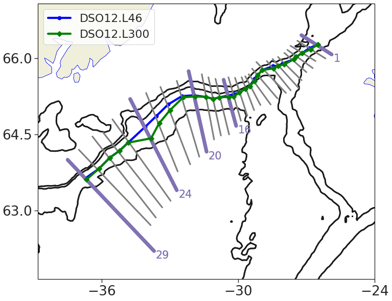
Figure B1 Overflow path. Contours show the 500, 1000, and 2000 m depth isobaths. The locations of the various sections used to monitor the model solution are indicated by grey and purple lines. The blue and green dots indicate for each section the location of the centre of the vein of the DSO in the control simulation (blue, DSO12.L46) and in the 1∕12^∘ 300-level simulation (green, DSO12.L300); the blue and green lines show the path of the overflow in these simulations.