the Creative Commons Attribution 4.0 License.
the Creative Commons Attribution 4.0 License.
 | 10 Jul 2020
Development of a two-way-coupled ocean–wave model: assessment on a global NEMO(v3.6)–WW3(v6.02) coupled configuration
Xavier Couvelard
Florian Lemarié
Guillaume Samson
Jean-Luc Redelsperger
Fabrice Ardhuin
Rachid Benshila
Gurvan Madec
This paper describes the implementation of a coupling between a three-dimensional ocean general circulation model (NEMO) and a wave model (WW3) to represent the interactions of upper-oceanic flow dynamics with surface waves. The focus is on the impact of such coupling on upper-ocean properties (temperature and currents) and mixed layer depth (MLD) at global eddying scales. A generic coupling interface has been developed, and the NEMO governing equations and boundary conditions have been adapted to include wave-induced terms following the approach of McWilliams et al. (2004) and Ardhuin et al. (2008). In particular, the contributions of Stokes–Coriolis, vortex, and surface pressure forces have been implemented on top of the necessary modifications of the tracer–continuity equation and turbulent closure scheme (a one-equation turbulent kinetic energy – TKE – closure here). To assess the new developments, we perform a set of sensitivity experiments with a global oceanic configuration at resolution coupled with a wave model configured at resolution. Numerical simulations show a global increase in wind stress due to the interaction with waves (via the Charnock coefficient), particularly at high latitudes, resulting in increased surface currents. The modifications brought to the TKE closure scheme and the inclusion of a parameterization for Langmuir turbulence lead to a significant increase in the mixing, thus helping to deepen the MLD. This deepening is mainly located in the Southern Hemisphere and results in reduced sea surface currents and temperatures.
- Article
(10122 KB) - Full-text XML
- BibTeX
- EndNote


An accurate representation of ocean surface waves has long been recognized as essential for a wide range of applications from marine meteorology to ocean and coastal engineering. Waves also play an important role in the short-term forecasting of extratropical and tropical cyclones by regulating sea surface roughness (Janssen, 2008; Chen and Curnic, 2015; Hwang, 2015). More recently, the impact of waves on oceanic circulation at the global scale has triggered interest from the research and operational community (e.g., Hasselmann, 1991; Rascle and Ardhuin, 2009; D'Asaro et al., 2014; Fan and Griffies, 2014; Li et al., 2016; Law Chune and Aouf, 2018). In particular, surface waves are important for an accurate representation of air–sea interactions, and their effect on fluxes of mass, momentum, and energy through the wavy boundary layer must be taken into account in ocean–atmosphere coupled models. For example, the momentum flux through the air–sea interface has traditionally been parameterized using near-surface winds (typically at 10 m) and the atmospheric surface layer stability (Fairall et al., 2003; Large and Yeager, 2009; Brodeau et al., 2016). The physics of the coupling depend on the kinematics and dynamics of the wave field. This includes a wide range of processes from wind–wave growth, nonlinear wave–wave interaction, and wave–current interaction to wave dissipation. Such complex processes can only be adequately represented by a wave model.
Besides affecting the air–sea fluxes, waves define the mixing in the oceanic surface boundary layer (OSBL) via breaking and Langmuir turbulence. For example, Belcher et al. (2012) showed that Langmuir turbulence should be important over wide areas of the global ocean, more particularly in the Southern Ocean. In this region, they show that the inclusion of the effect of surface waves on the upper-ocean mixing during summertime allows for a reduction of systematic biases in the OSBL depth. Indeed, their large eddy simulations (LESs) suggest that under certain circumstances wave forcing can lead to large changes in the mixing profile throughout the OSBL and in the entrainment flux at the base of the OSBL. They concluded that wave forcing is always important when compared to buoyancy forcing, even in winter. Moreover, Polonichko (1997) and Van Roekel et al. (2012) emphasized the fact that the Langmuir cell intensity strongly depends on the alignment between the Stokes drift and wind direction. Langmuir turbulence is maximum when wind and waves are aligned and becomes weaker as the misalignment becomes larger. Li et al. (2017) highlighted that ignoring the alignment of wind and waves (i.e., assuming that wind and waves are systematically aligned) in the Langmuir cell parameterizations leads to excessive mixing, particularly in winter.
Most previous studies of the impact of ocean–wave interactions at the global scale have used an offline one-way coupling and included only parts of the wave-induced terms in the oceanic model governing equations (e.g., Breivik et al., 2015; Law Chune and Aouf, 2018). In this study, the objective is to introduce a new online two-way-coupled ocean–wave modeling system with great flexibility to be relevant for a large range of applications from climate modeling to regional short-term process studies. This modeling system is based on the Nucleus for European Modelling of the Ocean (NEMO; Madec, 2012) as the oceanic compartment and WAVEWATCH III® (hereinafter WW3; WAVEWATCH III® Development Group, 2016) as the surface wave component. NEMO and WW3 are coupled using the OASIS Model Coupling Toolkit (OASIS-MCT; Valcke, 2013; Craig et al., 2017), which is widely used in the climate and operational community. The various steps for our implementation are the following: (i) the inclusion of all wave-induced terms in NEMO, only neglecting the terms relevant for the surf zone, which is outside the scope here; (ii) modification of the NEMO subgrid-scale physics (including the bulk formulation) to include wave effects and a parameterization for Langmuir turbulence; (iii) development of the OASIS interface within NEMO and WW3 for the exchange of data between the models; and (iv) a test of the implementation based on a realistic global configuration at for the ocean and for the waves.
To go into the details of those different steps, the paper is organized as follows. The modifications brought to the oceanic model primitive equations, their boundary conditions, and the subgrid-scale physics to account for wave–ocean interactions are described in Sect. 2. This includes the addition of the Stokes–Coriolis force, the vortex force, and the wave-induced pressure gradient. In Sect. 3 our modeling system coupling the NEMO oceanic model and the WW3 wave model via the OASIS-MCT coupler is described in detail. Numerical simulations are presented in Sect. 4 using a global configuration at for the oceanic model and for the wave model. Using sensitivity runs, we assess those global configurations with particular emphasis on the impact of wave–ocean interactions on mixed layer depth, sea surface temperature and currents, turbulent kinetic energy (TKE) injection, and kinetic energy. Finally, in Sect. 5, we summarize our findings and provide overall comments on the impact of two-way ocean–wave coupling in global configurations at eddy-permitting resolution.
In order to set the necessary notations, we start by introducing the classical primitive equations solved by the NEMO ocean model. Note that between the two possible options to formulate the momentum equations, namely the so-called “vector-invariant” and “flux” forms, we present the first one here, which will be used for the numerical simulations in Sect. 4. With the horizontal velocity vector, ω the dia-surface velocity component, θ the potential temperature, ρ the density, ζ the relative vorticity, ph the hydrostatic pressure, and ps the surface pressure, the Reynolds-averaged equations (with 〈⋅〉 the averaging operator omitted here for simplicity) are as follows.
Here, k is a nondimensional vertical coordinate, the lateral derivatives ∂x and ∂y have to be considered along the model coordinate, and e3 is the vertical scale factor given by , where z is the local depth and ρ is given by an equation of state (Roquet et al., 2015). The necessary boundary conditions include a kinematic surface and bottom boundary condition, which can be expressed in terms of the vertical velocity w,
with η the height of the sea surface and (E−P) the mass flux across the sea surface due to precipitation and evaporation, a momentum surface boundary condition for the Reynolds stress vertical terms,
with a wind stress vector that represents the part of the stress that drives the ocean, and a dynamic boundary condition on the free surface leading to the continuity of pressure across the air–sea interface. The kinematic boundary conditions (6) for w(z=η) and translate into and . We do not explicitly include the boundary conditions for the tracer equations here since they are unchanged from classical primitive equation models in the presence of wave motions. As mentioned earlier, in Eqs. (1) to (5) prognostic variables have to be interpreted in an Eulerian mean sense even if the averaging operator is not explicitly included.
2.1 Modification of governing equations and boundary conditions
Asymptotic expansions of the wave effects based on Eulerian velocities (McWilliams et al., 2004) or Lagrangian mean equations (Ardhuin et al., 2008) lead to the same self-consistent set of equations for weak vertical current shears. These are further applied and discussed by Uchiyama et al. (2010), Bennis et al. (2011), Michaud et al. (2012), and Moghimi et al. (2013). The three-component Stokes drift vector is and is non-divergent at lowest order (Ardhuin et al., 2008, 2017b). The coupled wave–current equations for the Eulerian mean velocity and tracers in a vector-invariant form (the equivalent flux form is given in Appendix A) are as follows.
Here, wave-induced terms are represented with tildes. The and terms represent the sink–source of wave momentum due to breaking, bottom friction, and wave–turbulence interaction. These terms will be neglected since they are expected to play a significant role only in the surf zone. The other extra contributions to the momentum equations include the Stokes–Coriolis force 𝓦St−Cor, the vortex force 𝓦VF, and a wave-induced pressure 𝓦Prs:
where the terms involving horizontal derivatives of ω have been neglected in 𝓦VF. In 𝓦Prs, the term corresponds to a depth-uniform wave-induced kinematic pressure term1, while is a shear-induced three-dimensional pressure term2 associated with the vertical component of the vortex force. The vortex force contribution 𝓦VF can be further simplified by neglecting the terms involving the vertical shear. In particular, the vertical component of the vortex force is absorbed in a pressure term (that gives the Sshear term in the notations of Ardhuin et al., 2008). That particular term was neglected in Bennis et al. (2011) because of the generally weak vertical shears in the wave mixed layer. The effect of that term was also found to be much weaker than in shallow coastal environments, except in the surf zone. This assumption has the advantage of leaving the hydrostatic relation (Eq. 11) unchanged. Our implementation of wave-induced terms in NEMO is in line with Bennis et al. (2011) and corresponds to the simplified form of Eq. (12):
Because of geostrophy, it is obvious that the addition of the Stokes–Coriolis force requires the effect of the Stokes drift on the mass and tracer advection to be taken into account. Regarding the joint modification of the tracers and continuity equations, it is clear that constancy preservation is maintained (i.e., a constant tracer field should remain constant during the advective transport) and that an additional wave-related forcing must be added to the barotropic mode. The NEMO barotropic mode has been modified accordingly since the surface kinematic boundary condition (Eq. 6) in terms of vertical velocities w and associated now reads
to express the fact that there is a source of mass at the surface that compensates for the convergence of the Stokes drift; hence, the barotropic mode is
where , represents the bottom drag coefficients, and is the usual NEMO forcing term containing coupling terms from the baroclinic mode and slowly varying barotropic terms (including nonlinear advective terms) held constant during the barotropic integration to gain efficiency. In Eq. (13), and contain the additional wave-induced barotropic forcing terms corresponding to the vertical integral of the 𝓦St−Cor and 𝓦VF terms, which are also held constant during the barotropic integration. A thorough analysis of the impact of the additional wave-induced terms on energy transfers within an oceanic model can be found in Suzuki and Fox-Kemper (2016). Note, however, that the study of Suzuki and Fox-Kemper (2016) is based on the Craik–Leibovich equations, which are a special case of the more general wave-averaged primitive equations. Those sets of equations are equivalent to each other only at lowest order in vertical shear.
2.2 Computation and discretization of Stokes drift velocity profile
Reconstructing the full Stokes drift profile us in the ocean circulation model would require obtaining the surface spectra of the Stokes drift from the wave model. Instead, profiles are generally reconstructed considering a few important parameters, including the Stokes drift surface value and the norm of the Stokes volume transport . In Breivik et al. (2014, 2016), Stokes drift velocity profiles are derived under the deepwater approximation in the general form , with ke a depth-independent spatial wavenumber chosen such that the norm of the depth-integrated Stokes transport (assuming an ocean of infinite depth) is equal to . The functions 𝒮B14(z,ke) from Breivik et al. (2014) and 𝒮B16(z,ke) from Breivik et al. (2016) for are given by
with erfc the complementary error function. It can be easily shown that for an ocean of infinite depth, the vertical integrals of those functions are respectively equal to for 𝒮B16 and for 𝒮B14. Standard computations of Stokes drift in numerical models are done in a finite-difference sense; however, due to the fast decay of with depth, a finite-volume approach seems more adequate in this case.
Such a finite-volume interpretation of the Stokes drift velocity can also be found in Li et al. (2017) and Wu et al. (2019). The 𝒮B16 function is more adapted for this kind of approach since the primitive function only requires special functions available in the Fortran standard.
Since NEMO is discretized on an Arakawa C grid, the components of the Stokes drift velocity must be evaluated at cell interfaces, and a simple average weighted by layer thicknesses is used:
Note that no explicit computation of the vertical component of the Stokes drift is necessary since in Eqs. (7)–(11) only appears summed with ω such that the relevant variable is as a whole. This quantity is diagnosed from the continuity equation (Eq. 10, where the temporal evolution of vertical scale factors ∂te3 is given by the free-surface evolution when a quasi-Eulerian vertical coordinate is used; e.g., z⋆ or terrain-following coordinates).
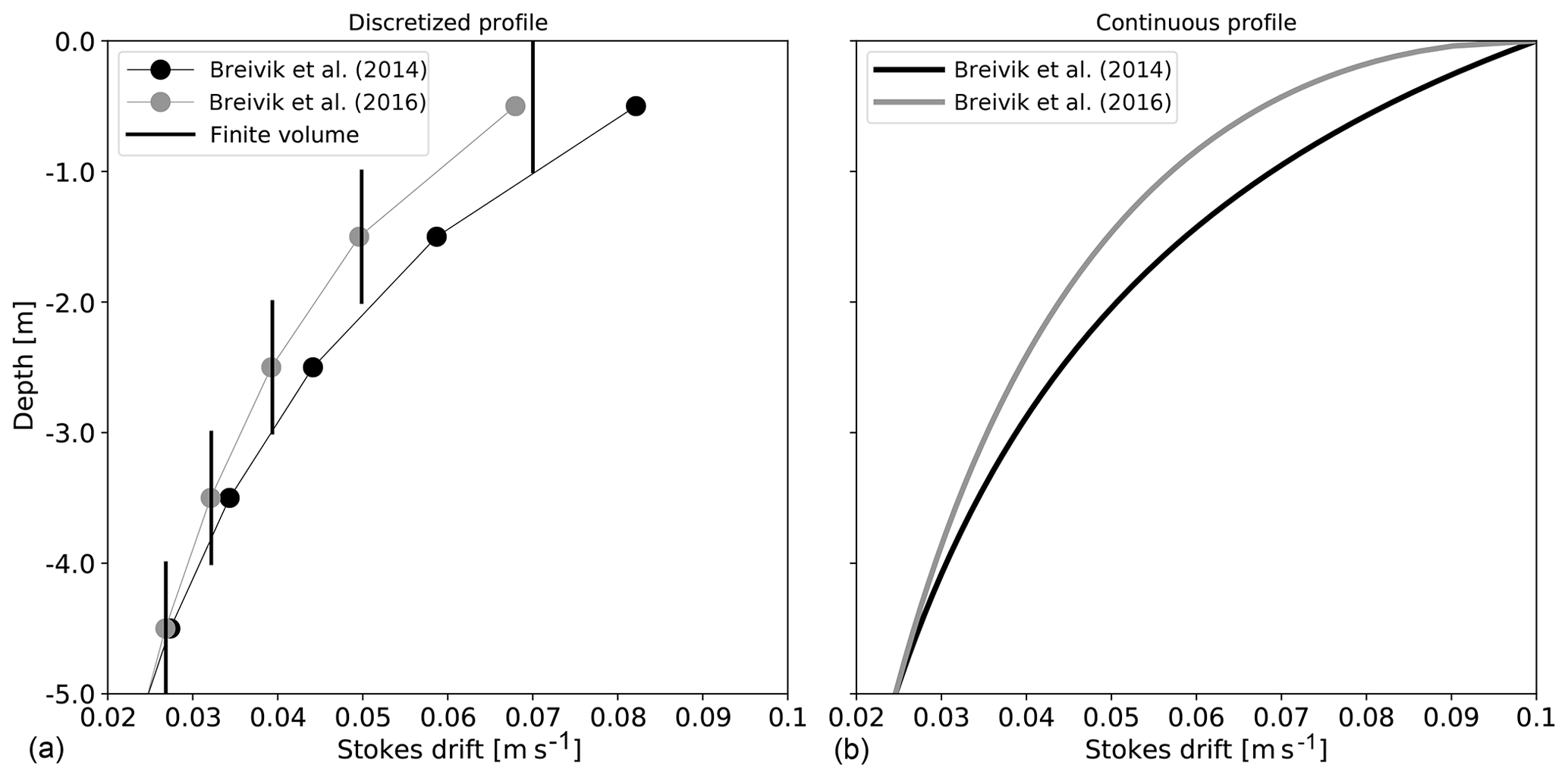
Figure 1(a) Reconstructed zonal component of a Stokes drift profile for m2 s−1, m s−1, and m s−1 for a 1 m resolution vertical grid using the Breivik et al. (2014) function (black dots), the Breivik et al. (2016) function (grey dots), and the finite-volume Breivik et al. (2016) function (black vertical lines). (b) Their continuous counterparts.
As illustrated in Fig. 1, for the typical vertical resolution used in most global models the properties of the discretized Stokes profiles can be very different from their continuous counterparts. Indeed, the 𝒮B16(z,ke) function has been considered superior to 𝒮B14(z,ke) because the vertical shear near the surface is expected to be better reproduced. However, in Fig. 1 it is shown that this is no longer the case at a discrete level since the discrete vertical gradients at 1 m of depth turn out to be larger for 𝒮B14(z,ke) compared to 𝒮B16(z,ke). In this case, the fast variations of 𝒮B16(z,ke) near the surface cannot be represented by the computational vertical grid. A vertical resolution finer than the one currently used in most global ocean models near the surface would be required to properly represent the Stokes drift shear.
2.3 Subgrid-scale physics
2.3.1 Turbulent kinetic energy prognostic equation and boundary conditions
Under the assumption of horizontal homogeneity generally retained in general circulation models, the contribution from Stokes drift to the turbulent kinetic energy (TKE) prognostic equation arises from the vortex force vertical term in the hydrostatic relation (Eq. 11). Mimicking the way the TKE equation is usually derived (see, e.g., Tennekes and Lumley, 1972) and using an averaging operator 〈⋅〉 satisfying the “Reynolds properties”, we find that the turbulent fluctuations, defined as , associated with the term are
After multiplication by w′ and averaging, we obtain
where the last two terms on the right-hand side cancel, with similar terms appearing when forming the equations for and (see Eqs. A.7 and A.8 in Skyllingstad and Denbo, 1995). The extra terms associated with the Stokes drift in the horizontally homogeneous TKE equation are thus and , which can be further rewritten as
The first term will modify the shear production term; it can also be derived by taking the Lagrangian mean of the wave-resolved TKE equation (Ardhuin and Jenkins, 2006). The second will enter the TKE transport term that is usually parameterized as . The prognostic equation for the turbulent kinetic energy e in NEMO under the assumption that Ke=Avm, with Avm the eddy viscosity, is thus
with Avt the turbulent diffusivity, N the local Brunt–Väisälä frequency, lε a dissipative length scale, and cε a constant parameter (generally such that ). Once the value of e is know, eddy diffusivity and viscosity are given by
with Prt the Prandtl number (see Sect. 10.1.3 in Madec, 2012, for the detailed computation of Prt), lm a mixing length scale, and Cm a constant.
In addition to the modification of the shear production term in the TKE equation, the wave will affect the surface boundary condition for e, lm, and lε. The Dirichlet boundary condition traditionally used in NEMO for the TKE variable is modified into a Neumann boundary condition,
meaning that the injection of TKE at the surface is given by the dissipation of the wave field via the wave–ocean Soce term, which is a sink term in the wave model energy balance equation usually dominated by wave breaking, converted into an ocean turbulence source term. In practice, this sum of Soce is obtained as a residual of the source term integration; hence, it also includes unresolved fluxes of energy to the high-frequency tail of the wave model. Due to the placement at cell interfaces of the TKE variable on the computational grid, the TKE flux is not applied at the free surface but at the center of the topmost grid cell (i.e., at z=z1). This amounts to interpreting the half-grid cell at the top as a constant flux layer, which is consistent with the surface layer Monin–Obukhov theory.
The length scales lm and lε are computed via two intermediate length scales lup and ldwn, respectively estimating the maximum upward and downward displacement of a water parcel with a given initial kinetic energy. lup and ldwn are first initialized to the length scale proposed by Deardorff (1980): . The resulting length scales are then limited not only by the distance to the surface and to the bottom but also by the distance to a strongly stratified portion of the water column such as the thermocline. This limitation amounts to controlling the vertical gradients of lup(z) and ldwn(z) such that they are not larger that the variations of depth (Madec, 2012)
Then, the dissipative and mixing length scales are given by and . Following Redelsperger et al. (2001) (their Sect. 4.2.3), a boundary condition consistent with the Monin–Obukhov similarity theory for the length scale ldwn (while lup necessitates only a bottom boundary condition) is
with κ the von Karman constant and Cm and cε the constant parameters in the TKE closure. The surface roughness length z0 can be directly estimated from the significant wave height provided by the wave model as z0=1.6Hs (Rascle et al., 2008, their Eq. 5), which provides a proxy for the scale of the breaking waves. Note that in our study, no explicit parameterization of the mixing induced by near-inertial waves has been added (Rodgers et al., 2014). As highlighted by Breivik et al. (2015), without activating this ad hoc parameterization in the standard NEMO TKE scheme, the model does not mix deeply enough. They also speculated that this ad hoc mixing could mask the effects of wave-related mixing processes such as Langmuir turbulence. For this reason, it is not used in the present simulations.
2.3.2 Langmuir turbulence parameterization
Langmuir mixing is parameterized following the approach of Axell (2002). This parameterization takes the form of an additional source term PLC in the TKE equation (15). PLC is defined as
where wLC represents the vertical velocity profile associated with Langmuir cells and dLC their expected depth. Following Axell (2002), wLC and dLC are given by
where is the portion of the surface Stokes drift contributing to Langmuir cell intensity and cLC a constant parameter. In the absence of information about the wave field it is generally assumed that . As mentioned in the Introduction, Polonichko (1997) and Van Roekel et al. (2012) showed that the intensity of Langmuir cells is largely influenced by the angle between the Stokes drift and the wind direction. To reflect this dependency we account for this angle in our definition of via
with eτ the unit vector in the wind stress direction. The difference between the surface Stokes drift and given by Eq. (17) is shown in Fig. 2 and compared to the usual parameterization of as in the uncoupled case (see Madec, 2012). The modulation of depending on the wind stress orientation significantly reduces the input of the surface Stokes drift contributing to Langmuir cell intensity, especially in the Southern Ocean, while other regions are less affected. Finally, a value for the parameter cLC must be chosen. Based on single-column experiments detailed in Appendix B, we find that parameter values in the range 0.15–0.3 provide satisfactory results compared to the LESs of Noh et al. (2016) and will be considered for the numerical experiments discussed later in Sect. 4.2.
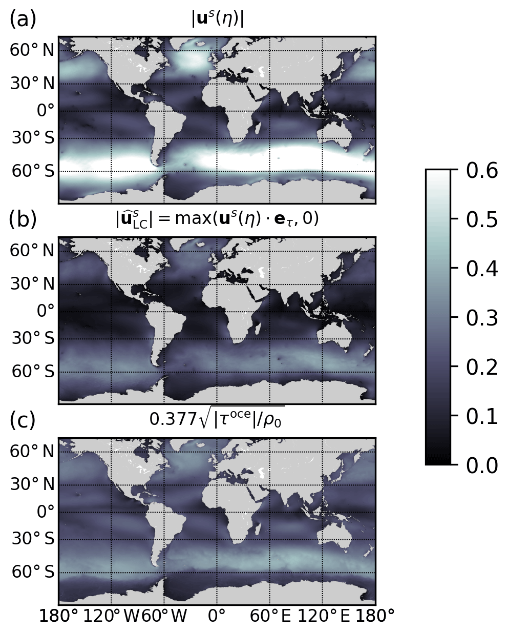
Figure 2Annual average of the surface Stokes drift module (m s−1) (a), the portion of the Stokes drift aligned with the wind, as given in Eq. (17) (b), and the surface Stokes drift as parameterized by in the uncoupled case (c).
While the Axell (2002) parameterization was already implemented in NEMO, there are three major novelties in our implementation: (i) the online coupled strategy allows us to use the surface Stokes drift directly delivered by the wave model instead of the original value empirically estimated from the wind speed (e.g., 1.6 % of the 10 m wind). (ii) We only considered the component of the Stokes drift aligned with the wind, and (iii) based on a series of single-column simulations (see Appendix B) the coefficient cLC evaluated as 0.15 by Axell (2002) is set to a 0.3 value. Those changes, together with the new surface boundary condition for the TKE equation, lead to a deeper penetration of the TKE inside the mixed layer and, as shown in Sect. 4.2.3, greatly improved the MLD distribution.
Our coupled model is based on the NEMO oceanic model, the WW3 wave model, and the OASIS library for data exchange and synchronization between the two components.
3.1 Numerical models and coupling infrastructure
The ocean model: NEMO
NEMO is a state-of-the-art primitive-equation, split–explicit, free-surface oceanic model whose equations are formulated both in the vector-invariant and flux forms (see Eq. 1 for the vector-invariant form). The equations are discretized using a generalized vertical coordinate featuring, among others, the z⋆ coordinate with partial-step bathymetry and the σ coordinate, as well as a mixture of both (Madec, 2012). For efficiency and accuracy in the representation of external gravity wave propagation, model equations are split between a barotropic mode and a baroclinic mode to allow the possibility to adopt specific numerical treatments in each mode. The NEMO equations are spatially discretized on an Arakawa C grid in the horizontal and a Lorenz grid in the vertical, and the time dimension is discretized using a leapfrog scheme with a modified Robert-Asselin filter to damp the spurious numerical mode associated with leapfrog (Leclair and Madec, 2009). For the current study the NEMO equations have been modified to include wave effects as described in Eqs. (7) and (13). Moreover, the modifications to the standard NEMO one-equation TKE closure scheme are given in Sect. 2.3.
The wave model: WW3
The NEMO ocean model has been coupled to the WW3 wave model. In numerical models, waves are generally described using several phase and amplitude parameters. We provide only the details sufficient to understand the coupling of waves with the oceanic model here, and an exhaustive description of WW3 is given by WAVEWATCH III® Development Group (2016). WW3 integrates the wave action equation (Komen et al., 1994) with the spectral density of wave action Nw(kw,θw) discretized in wavenumber kw and wave propagation direction θw for the spectral space (the subscript w is used here to avoid confusion with previously introduced notations):
where λ is longitude, ϕ is latitude, and S is the net spectral source term that includes the sum of the rate of change of the surface elevation variance due to interactions with the atmosphere via wind–wave generation and swell dissipation (Satm), nonlinear wave–wave interaction (Snl), and interaction with the upper ocean that is generally dominated by wave breaking (Soce). Those parameterized source terms are important in wave–ocean coupling. Indeed, as shown earlier in Eq. (16), the Soce term is used to compute the TKE flux transmitted to the ocean, and the Sin term enters the computation of the wave-supported stress. They are computed here following Ardhuin et al. (2010b). In Eq. (18), the dot variables correspond to a propagation speed given by the following.
Here, R is the Earth's radius, represents the surface currents provided by the ocean model, cg is the group velocity, ωw the absolute radian frequency, and H the mean water depth. Equation (18) is solved for each spectral component (kw,θw) coupled by the advection and source terms. Equations (19)–(22) show how the oceanic currents affect the advection of the wave action density; there are also indirect effects via the source term (Ardhuin et al., 2009).
The coupler: OASIS-MCT
The practical coupling between NEMO and WW3 has been implemented using the OASIS-MCT (Valcke, 2013; Craig et al., 2017) software primarily developed for use in multicomponent climate models. This software provides the tools to couple various models at low implementation and performance overhead. In particular, thanks to MCT (Jacob et al., 2005), it includes the parallelization of the coupling communications and runtime grid interpolations. For efficiency, interpolations are formulated in the form of a matrix–vector multiplication whereby the matrix containing the mapping weights is computed offline once for all. In practice, after compiling OASIS-MCT, the resulting library is linked to the component models so that they have access to the specific interpolation and data exchange subroutines. Now that we have described the different components involved in our coupled system, we go into the details of the nature of the data exchanged between both models.
3.2 Oceanic surface momentum flux computation
Surface waves affect the momentum exchange between the ocean and the atmosphere in two different ways. First, the modification of surface roughness acts on the incoming atmospheric momentum flux τatm. Second, a part of the momentum flux from the atmosphere is consumed by the wave field and contributes to the growing waves (the so-called wave-supported stress); conversely, the waves release momentum to the ocean when they break and dissipate. This implies that the wind stress transferred to the oceanic model (we call it τoce) is different from the atmospheric wind stress τatm. These two coupling processes are taken into account in our coupled framework.
The 10 m wind is sent to the wave model, which internally computes the dimensionless Charnock parameter αch characterizing the sea surface roughness (Charnock, 1955; Janssen, 2009). This information is used by the wave model to compute its own atmospheric wind stress assuming neutral stratification, i.e., with CDN a neutral drag coefficient, which is function of the Charnock parameter. Then the wave model computes the momentum flux transferred to the ocean . Using the latest available values of αch, , , and , the oceanic model computes an atmospheric wind stress τatm using its own bulk formulation, and the local value of the momentum flux going into the water column is diagnosed as
where the τww3 quantities are interpolated from the wave grid to the oceanic grid. In NEMO, the wind stress is computed using the IFS (Integrated Forecasting System: https://www.ecmwf.int/en/forecasts/documentation-and-support/changes-ecmwf-model/ifs-documentation, last access: 2 July 2020) bulk formulation such as implemented in the AeroBulk (https://github.com/brodeau/aerobulk, last access: 2 July 2020) package (Brodeau et al., 2016). In particular, the roughness length that enters the definition of the drag coefficient is a function of the Charnock parameter αch,
where αm=0.11, u⋆ is the friction velocity, and ν the air kinematic viscosity whose contribution is significant only asymptotically at very low wind speed. Note that in the uncoupled case the default value of the Charnock parameter is . In our implementation, the momentum fluxes are computed using the absolute wind at 10 m rather than the relative wind . Indeed, several recent studies have emphasized that the use of relative winds is relevant only when a full coupling with an atmospheric model is available since in a forced mode it leads to an unrealistically large loss of oceanic eddy kinetic energy (e.g., Renault et al., 2016). This is not a limitation of our approach since a simple modification of a namelist parameter allows us to run with relative winds, but this case is not investigated in the present study.
In our coupling strategy two different values of the atmospheric wind stress and the wave-to-ocean wind stress are computed with two different bulk formulations. This strategy is not fully satisfactory since it breaks the momentum conservation. However, it was necessary in practice since the WW3 results were very sensitive to the bulk formulation, and at the same time it was not conceivable to use the WW3 bulk formulation to force the ocean model because the latter ignores the effect of stratification in the atmospheric surface layer. Previous implementations in NEMO (e.g., Breivik et al., 2015; Alari et al., 2016; Staneva et al., 2017; Law Chune and Aouf, 2018; Wu et al., 2019) assumed that the wave field only acts on the norm of τatm and not on its orientation. Instead of Eq. (23), the atmospheric wind stress was corrected as follows.
However, this approach potentially leads to artificially large values of τoce when is small, and it does not take into account the slight change in τoce direction induced by the waves.
3.3 Additional details about the practical implementation
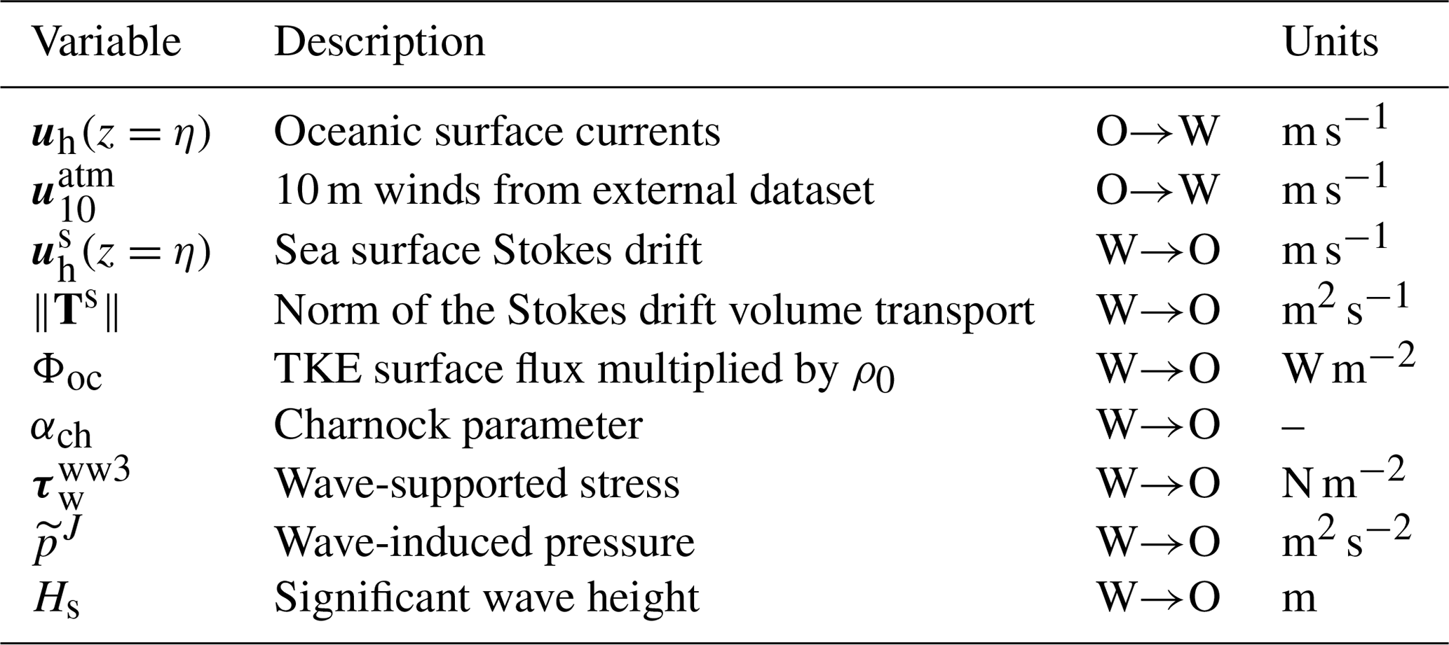
In Table 1 the different variables exchanged between the oceanic and wave models are given. All variables are 2D variables, meaning that no 3D arrays are exchanged through the coupler. All 2D interpolations are made through a distance-weighted bilinear interpolation. The time discretization steps Δtww3 for WW3 and Δtnemo for NEMO are generally different with Δtww3>Δtnemo and chosen such that Δtww3=ntΔtnemo (). In this case, coupling fields from NEMO to WW3 are averaged in time between two exchanges, while fields from WW3 to NEMO are sent every Δtww3 steps and therefore updated every nt time steps in NEMO. If Δtww3>Δtnemo, the coupler time step is set to Δtww3. Our current implementation does not include an explicit coupling between waves and sea ice, while it is known that waves lead to ice breakup, pancake ice formation, and associated enhancement of both freezing and melting; in return, this wave dissipation in ice-covered water (e.g., Stopa et al., 2018) leads to ice drift. Such explicit coupling is currently under development within the NEMO framework (Boutin et al., 2019).
Table 1Variables exchanged between NEMO (O) and WW3 (W) via the OASIS-MCT coupler. The 10 m wind is interpolated online by WW3 and does not go through the OASIS-MCT coupler.
4.1 Experimental setup and experiments
4.1.1 The global coupled ORCA25 configuration
The wave hindcasts presented here are all based on the WW3 model in its version 6.02 configured with a single grid at 0.5∘ resolution in longitude and latitude. A spectral grid with 24 directions and 31 frequencies is exponentially spaced over the interval with Hz and Hz. A one-step monotonic third-order coupled space–time advection scheme (also called the ultimate quickest scheme) is used with a specific procedure to alleviate the so-called garden sprinkler effect (Tolman et al., 2002). As suggested in Phillips (1984), the dissipation induced by wave breaking is proportional to the local saturation spectrum (see also Ardhuin et al., 2010a; Rascle and Ardhuin, 2013). The wind input growth rate at high frequency is based on the formulation of Janssen (1991) with an additional “sheltering” term to reduce the effective winds for the shorter waves (Chen and Belcher, 2000; Banner and Morison, 2010). For the computation of nonlinear wave–wave interactions, the discrete interaction approximation of Hasselmann et al. (1985) is used. This last approximation is known to be inaccurate, but it is thought that the associated errors are usually compensated for by a proper adjustment of the dissipation source term (Banner and Young, 1994; Ardhuin et al., 2007). As mentioned earlier in Sect. 3.2, the model was run with 10 m winds, without any air–sea stability correction. No wave measurements were assimilated in the model, but the stand-alone wave model was developed based on spectral buoy and synthetic aperture radar (SAR) data (Ardhuin et al., 2010b) and calibrated against altimeter data by adjusting the wind–wave coupling parameter (Rascle and Ardhuin, 2013). The WW3 time step for the global configurations is Δtww3=3600 s.
For the oceanic component, we use a global ORCA025 configuration at a horizontal resolution (Barnier et al., 2006). The vertical grid is designed with 75 vertical z levels with vertical spacing increasing with depth. Grid thickness is about 1 m near the surface and increases with depth to reach 200 m at the bottom. Partial steps are used to represent the bathymetry. The LIM3 sea ice model is used for the sea ice dynamics and thermodynamics (Rousset et al., 2015). The vertical mixing coefficients are obtained from the one-equation TKE scheme described in Sect. 2.3, and the convective processes are mimicked using an enhanced vertical diffusion parameterization that increases vertical diffusivity to 10 m2 s−1 at which static instability occurs. Water density is computed from temperature and salinity through the use of a polynomial formulation of the UNESCO (1983) nonlinear equation of state (Roquet et al., 2015). The vector-invariant form of momentum advection uses Arakawa and Lamb (1981) for the vorticity and a specific formulation to control the Hollingsworth instability (Ducousso et al., 2017). Momentum lateral viscosity is biharmonic and acts along geopotential surfaces. It is set to a value of 1.5×10¹¹ m4 s−1 at the Equator and varies proportionally to Δx3 away from the Equator. Advection of tracers is performed with a flux-corrected transport (FCT) scheme (Lévy et al., 2001), and lateral diffusion of tracers is harmonic and acts along an iso-neutral surface. It is set to a value of 300 m2 s−1 at the Equator, which varies proportionally to Δx. The bottom friction is nonlinear and the lateral boundary condition is free-slip. In this setup, the baroclinic time step is set to Δtnemo=900 s and a barotropic time step 30 times smaller. Compared to the standard uncoupled ORCA025 configuration, the additional computational cost associated with WW3 and the exchanges through the coupler is about 20 %.
4.1.2 Atmospheric forcings
The atmospheric fields used to force both ocean and wave models are based on the ECMWF (European Centre for Medium-Range Weather Forecasts) ERA-Interim reanalysis (Dee et al., 2011). Corrections have been applied to guarantee that the ERA-Interim mean states for rainfall as well as shortwave and longwave radiative fluxes are consistent with satellite observations from the Remote Sensing Systems (RSS) Passive Microwave Water Cycle (PMWC) product (Hilburn, 2009) and GEWEX SRB 3.1 data (https://gewex-srb.larc.nasa.gov/, last access: 2 July 2020). Momentum and heat turbulent surface fluxes are computed using the IFS bulk formulation from the AeroBulk package (Brodeau et al., 2016) using air temperature and humidity at 2 m, mean sea level pressure, and 10 m winds.
4.1.3 Sensitivity experiments and objectives
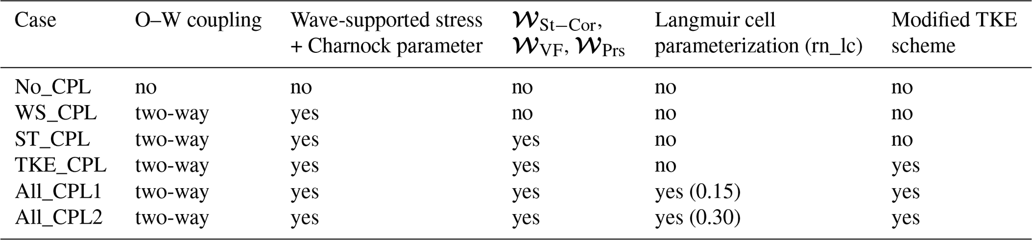
Sensitivity experiments have been conducted to check the proper implementation of various components of the present coupled modeling system. For the sake of clarity, our developments are split into four components: (i) the modification of the wind stress by waves through the Charnock parameter and the inclusion of wave-supported stress, (ii) the modifications of the NEMO governing equations through the Stokes–Coriolis, vortex force, and wave-induced surface pressure terms, (iii) the addition of a Langmuir turbulence parameterization, and (iv) the modifications to the TKE scheme. As summarized in Table 2, sensitivity experiments are designed in such a way to incrementally increase the level of complexity and test the effect of each component. The No_CPL experiment corresponds to the classical NEMO setup in which the wave effect is parameterized through a wind-stress-dependent TKE surface boundary condition as suggested by Craig and Banner (1994). In this approach, a Dirichlet surface boundary condition is used and expressed as follows: with αCB=100. Based on the results of Mellor and Blumberg (2004) we expect that in the uncoupled case the nature of the boundary condition (i.e., Dirichlet vs. Neumann) does not significantly impact numerical solutions3. The WS_CPL experiment is identical as No_CPL except that the wave coupling is introduced within the wind stress computation, as described in Sect. 3.2. The ST_CPL experiment is as WS_CPL except that all terms relative to the Stokes drift described in Sect. 2.1 are added in NEMO. TKE_CPL corresponds to ST_CPL but with the modified TKE scheme described in Sect. 2.3.1. All_CPL (1 and 2) experiments are like TKE_CPL but with a fully modified TKE scheme including the Langmuir cell parameterization described in Sect. 2.3.2. All those simulations have been performed for 2 years (2013–2014), during which 2013 is spin-up and only 2014 is analyzed. We considered 2 years sufficient to illustrate the fact that our developments were actually producing the expected results. Integrating longer in time could also lead to drifts in the stratification independently from the wave effects and could thus distort our interpretation. In any case, it must be clear that the objective here is not to go through a thorough physical analysis of coupled solutions but to check and validate our numerical developments.
4.2 Numerical results
4.2.1 Wave impact on oceanic wind stress
The wave distribution being inhomogeneous on the globe, it is expected that with the wave-modified wind stress parameterization the stress should follow the wave patterns more closely. In Fig. 3, the seasonal average of the significant wave height and of the difference between the Charnock coefficient computed by the wave model and the default constant value used in the uncoupled case () are shown. As expected, the Charnock parameter tends to be stronger in the area where the waves are higher. Generally an increase in the Charnock parameter is observed in the northern and southern basin, while there is a net decrease in αch near the Equator. There is also a strong seasonality in the Northern Hemisphere, with a reduction in summer and a strong increase in winter. The differences between αch and are very latitudinal with very few longitudinal variations.
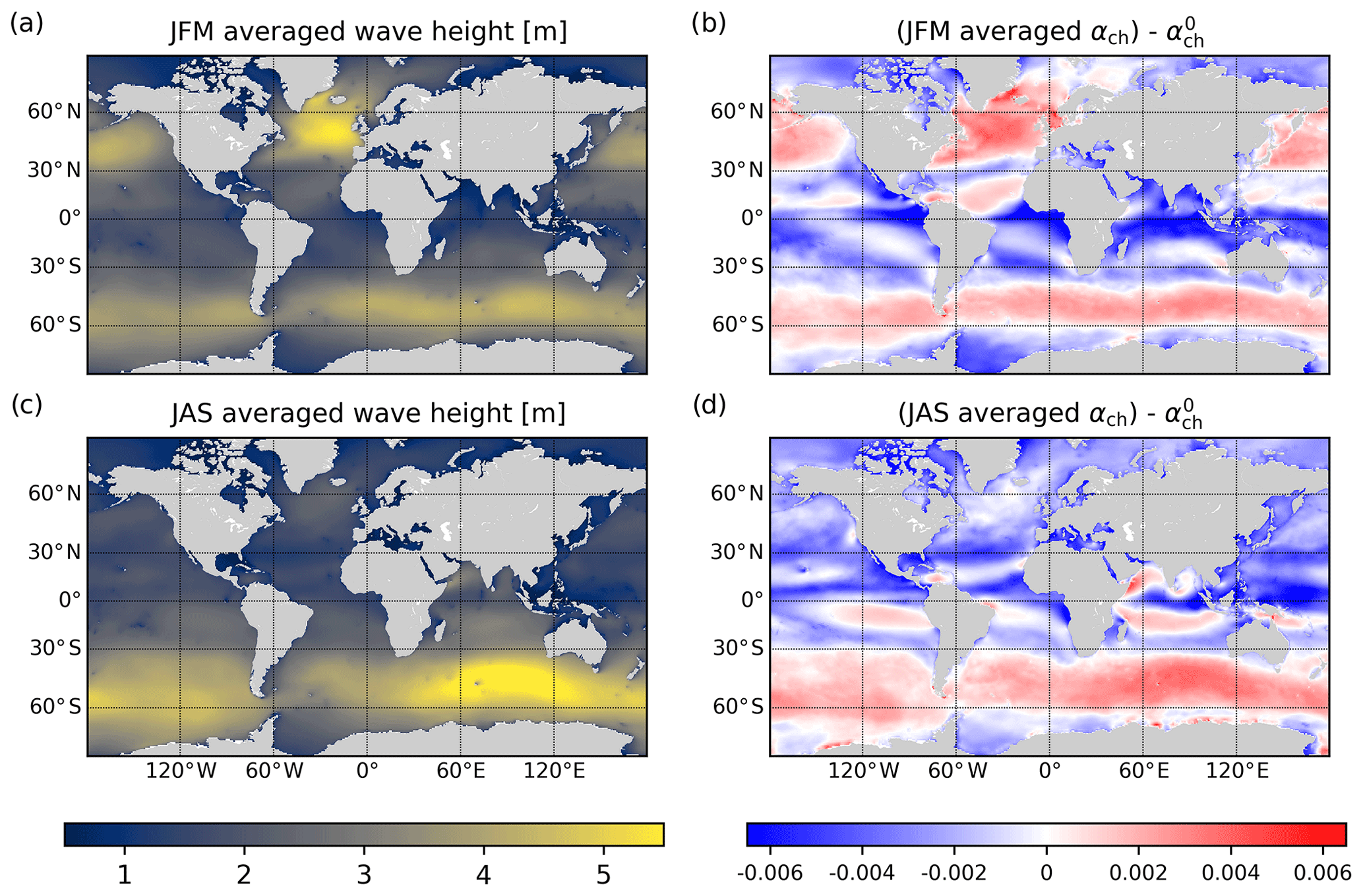
Figure 3(a, c) Seasonal averages of significant wave height (in meters) for January–February–March (JFM, panel a) and July–August–September (JAS, panel c). (b, d) Seasonal average of the difference between the Charnock parameter as computed by the wave model and the default value for JFM (b) and JAS (d).
To isolate the effect of the Charnock parameter we compare the results obtained in the No_CPL and WS_CPL experiments. Those two experiments show relatively similar sea surface temperature patterns, meaning that the modification of the wind stress between those two cases is primarily due to the use of different Charnock parameters and the inclusion of the wave-supported stress.
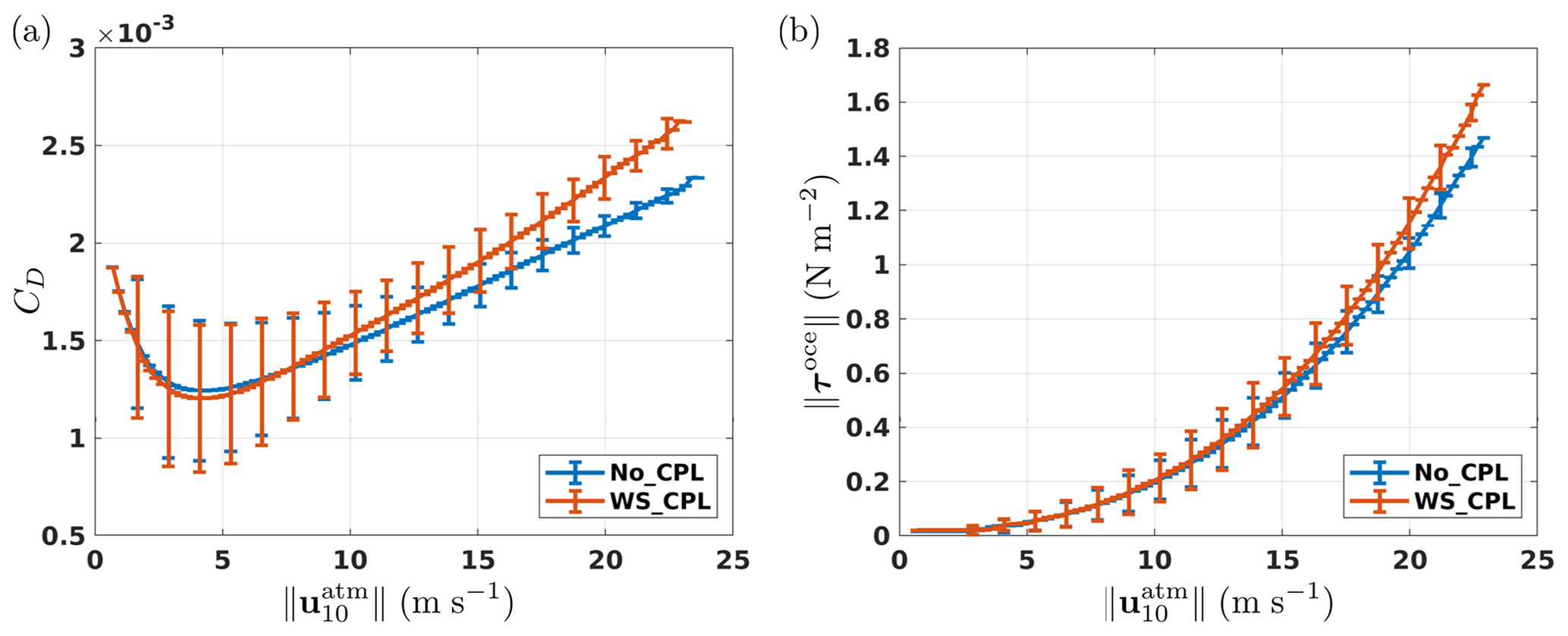
Figure 4(a) Drag coefficient (CD) as a function of the 10 m wind speed and (b) wind stress norm as a function of (black curves represent the mean value, while the vertical bars represent the standard deviation).
Figure 4a illustrates that the Charnock parameter mostly affects the drag coefficient CD, and hence the surface wind stress, for large winds. The ocean–wave coupling does not lead to appreciable differences in the drag coefficient CD for wind speeds lower than 8 m s−1. On the contrary, since large values of the Charnock parameter are observed for large wind speeds, the coupling significantly increases the drag (as well as its variance) at high winds. Figure 4b shows how the wind stress is modified by this increase in the drag coefficient jointly with the wave-supported stress, which tends to decrease the wind stress magnitude (Fig. 5). At low wind speed the wind stress magnitude is not affected by the coupling with waves, while for strong winds the increase in wind stress associated with the increased drag coefficient is always larger than the decrease associated with the wave-supported stress. This latter effect reduces the wind stress by no more than 2 %; for the characteristic scales of our study, this correction is thus almost negligible. The wind stress changes due to the coupling with waves seen in our simulations are very localized in time and space and it is thus difficult to conclude on their overall effect on upper-ocean dynamics such as Ekman pumping and the surface currents.

Figure 5Wind stress difference (N m−2) due to the correction made for growing waves for the WS_CPL experiment as a function of the 10 m wind speed.
4.2.2 Wave impact on surface TKE injection
As described in Sect. 2.3, in the ocean–wave coupled case, the surface boundary condition for the TKE equation is a Neumann condition whose value is directly given by the wave model, unlike the uncoupled case in which a Dirichlet condition is imposed. We aim here to assess the impact on the order of magnitude of the near-surface TKE. Since the Neumann boundary condition is applied at the center of the topmost grid box (i.e., approximately at 50 cm of depth), we compare in Fig. 6 the TKE value at 1 m of depth between the coupled (All_CPL2) and the uncoupled (No_CPL) case. Positive values mean that near-surface TKE is larger in the coupled simulation.
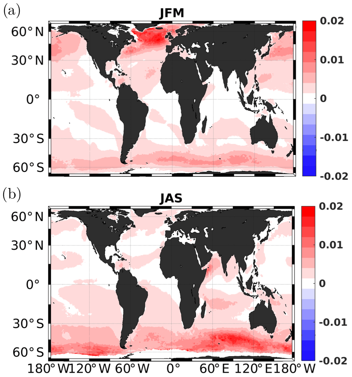
Figure 6Seasonal difference of 1 m depth turbulent kinetic energy (m2 s−2) between the coupled case (All_CPL2) and the uncoupled case (No_CPL). (a) January, February, and March (JFM); (b) July, August, and September (JAS).
It shows an almost homogeneous increase in the TKE (up to more than 100 %) in the extratropical areas. While low seasonal variability in the extratropical areas is visible in Fig. 6, a spatial averaging by hemisphere (Fig. 7) highlights seasonal variability with a strong increase in both the near-surface TKE value and the TKE difference between the two experiments during winter. In Figs. 6 and 7 (and also in the remainder of the paper), the spatial averaging is made between 25 and 60∘ S in the Southern Hemisphere and between 25 and 60∘ N in the Northern Hemisphere to avoid any conflicts with sea ice and to remove the equatorial region from the comparison. The increase in the surface TKE injection associated with waves is expected to contribute to an overall increase in mixed layer depth provided that the mixing length diagnosed by the turbulent closure scheme allows for the effective propagation of this additional TKE deeper in the mixed layer.
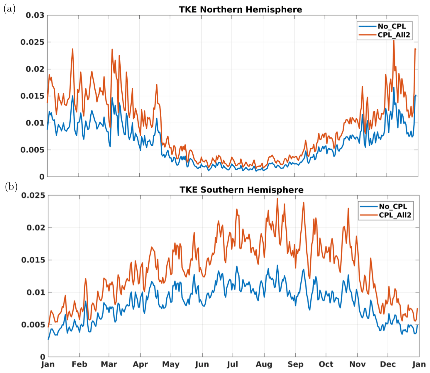
Figure 7Spatially averaged turbulent kinetic energy (m2 s−2) at 1 m of depth over (a) the Southern Hemisphere and (b) the Northern Hemisphere.
4.2.3 Wave impact on mixed layer depth
In this section, we evaluate the wave effect on vertical mixing using the mixed layer depth (MLD) as a relevant metric. Figure 8 represents the seasonally averaged difference in MLD between the coupled (All_CPL2) and the uncoupled (No_CPL) case relative to the No_CPL case (i.e., with hMLD considered negative downward). It shows a significant deepening of the mixed layer at high latitudes in the coupled case with only a very few localized mixed layer shallowing up to 60 %, mainly in the Southern Hemisphere.
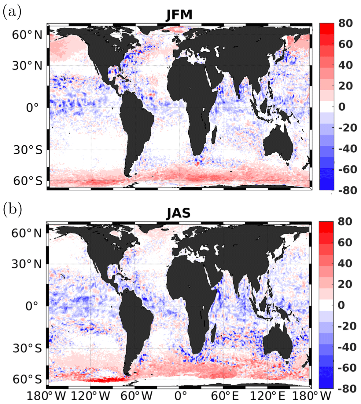
Figure 8(a, b) Seasonally averaged MLD differences (All_CPL2-No_CPL) relative to the uncoupled simulation No_CPL. Red corresponds to a deeper MLD for All_CPL2.
To assess whether the overall deepening of the mixed layer is realistic, we make a comparison with available observations. Available observations for 2014 were extracted following an updated dataset from de Boyer Montégut et al. (2004). The MLD has been computed as the depth at which the density is 3 % smaller that the density at 10 m as in de Boyer Montégut et al. (2004). Figure 9 represents the spatially averaged MLD; the blue line is the spatially averaged MLD obtained from ARGO floats (available during the same period) in both hemispheres. In the Northern Hemisphere (Fig. 9a), there is only a slight improvement compared to data during winter and late summer when implementing the coupling with waves. In the Southern Hemisphere (Fig. 9b) the situation is rather different.
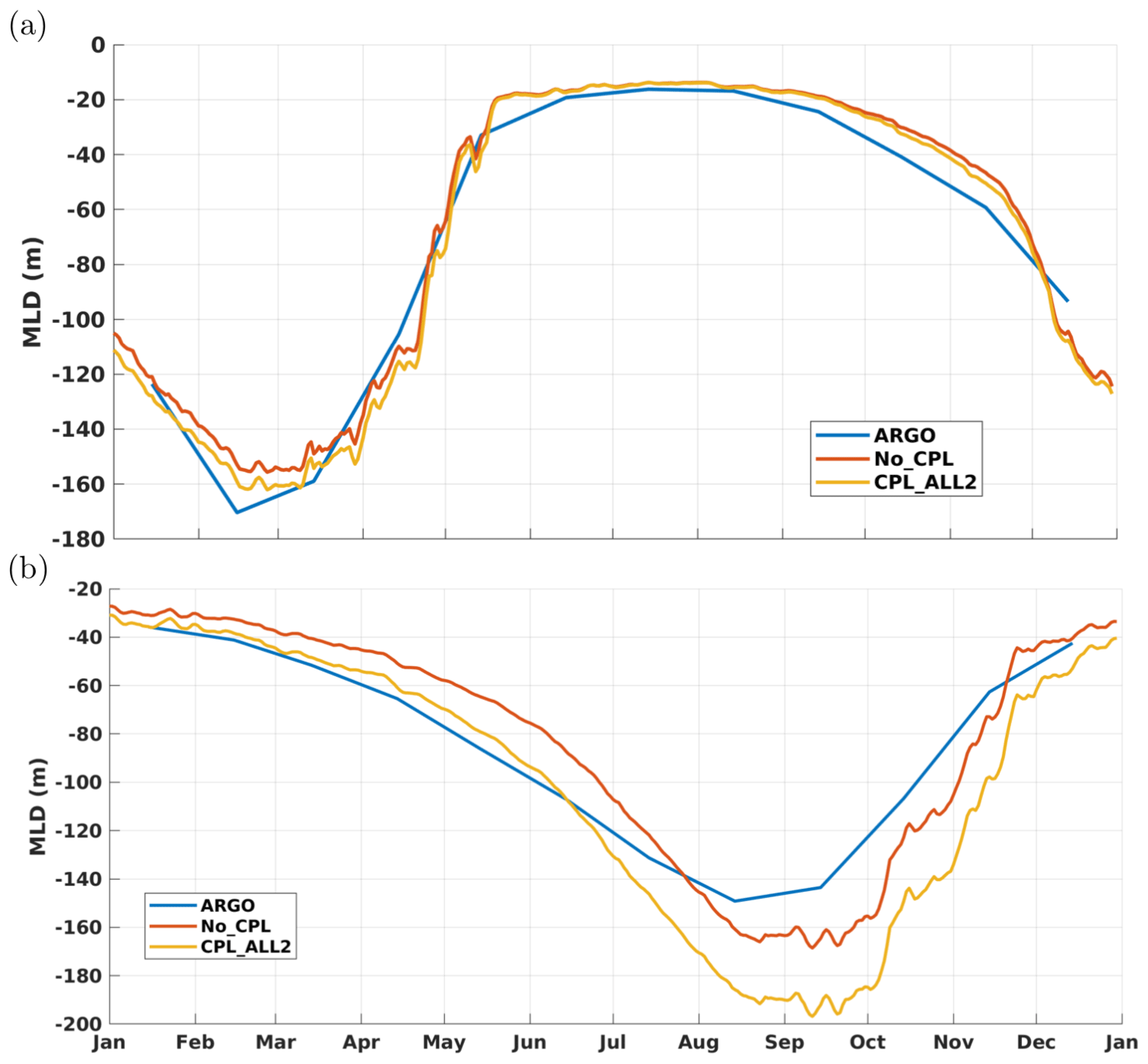
Figure 9Spatially averaged MLD for (a) the Northern Hemisphere and (b) the Southern Hemisphere.
From January to July, the deepening of the MLD induced by the wave coupling significantly reduces the bias between the model and ARGO data. From July to December, results in the coupled case show an overestimation of MLDs, which were already too deep in the uncoupled case, thereby increasing the bias between the data and model. Since mesoscale activity makes direct comparisons to data unreliable for such a short period of time, we compare the normalized distribution of MLD between the different simulations and available ARGO data. Results are presented in Fig. 10 for the year 2014 (panel a) and during summer only (panel b). In both cases the improvement in the Northern Hemisphere is very modest. As far as the Southern Hemisphere is concerned the coupling with waves leads to a significant improvement compared to the MLD derived from ARGO floats despite the fact that there are still too many low MLD values in the range 50–100 m. In comparison with the uncoupled case there is a more realistic spreading toward deeper mixed layer depths. More particularly in summer (Fig. 10b), the probability density function (PDF) in the coupled case matches the one computed from ARGO data almost perfectly. Despite the fact that we did not activate the ad hoc extra mixing induced by near-inertial waves (Rodgers et al., 2014), our implementation of the wave–ocean interaction leads to a significant deepening of the MLD in a realistic way.
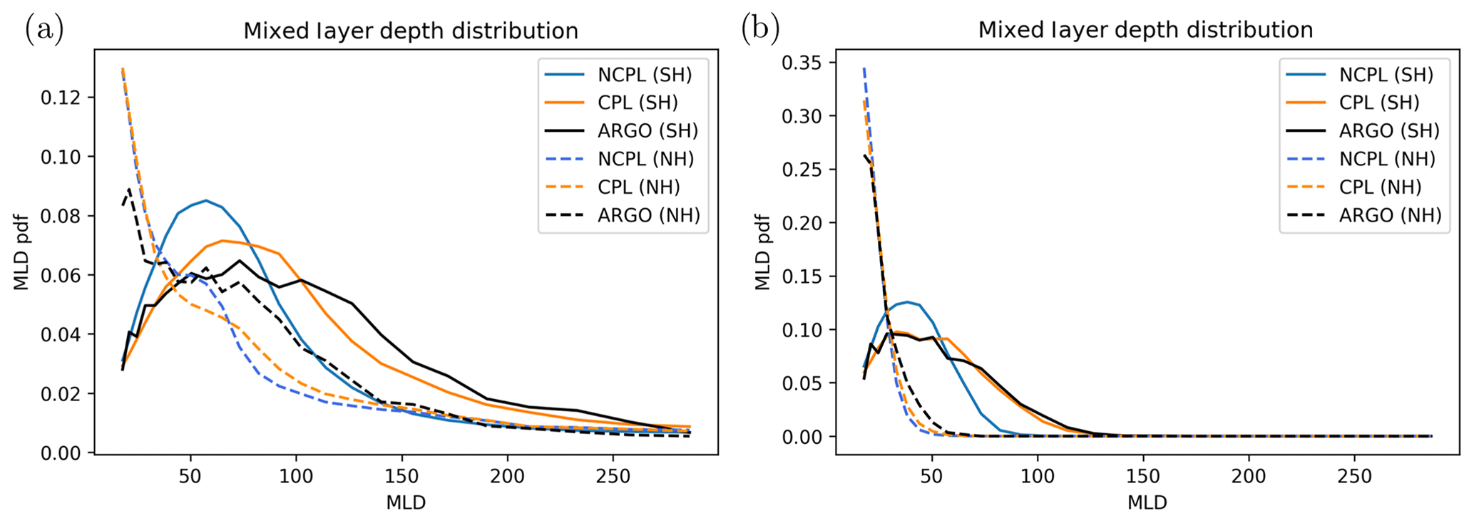
Figure 10Mixed layer depth probability density function for (a) the full 2014 year and (b) summer 2014.
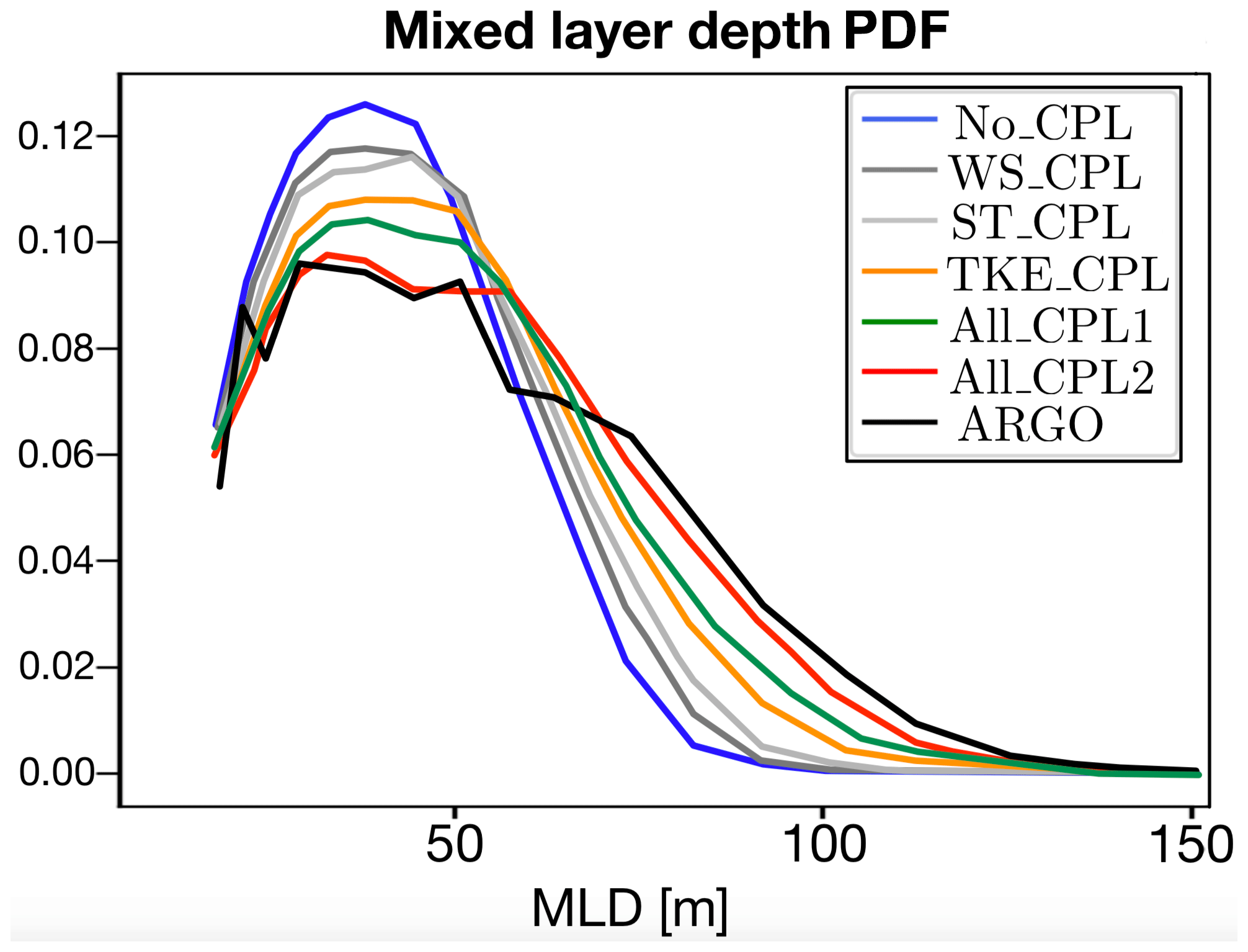
To better understand which components of the wave–ocean coupling are responsible for this improvement, the summer PDF in the Southern Hemisphere has been computed for each of the experiments described in Table 2. Results are shown in Fig. 11. First of all, it can be seen that all the wave–ocean interactions described in previous sections lead to an improvement in terms of mixed layer depth distribution compared to the uncoupled case. Indeed, the modification of the wind stress by the wave field introduced in WS_CPL increases both surface currents and near-surface TKE values, resulting in a slight deepening of the MLD. Adding the Stokes-drift-related terms in the primitive equations contributes only modestly to the deepening of the MLD, while most of the improvement results from the modified TKE scheme, with some slight improvement when the Langmuir parameterization is activated. It is somewhat reassuring to see that the better agreement with ARGO data is obtained when all components of the coupling are activated.
4.2.4 Wave impact on sea surface temperature
Since the near-surface mixing is strengthened by the coupling, we can expect an impact on sea surface temperature (SST). Figure 12 represents the time series of SST for each hemisphere. The Northern Hemisphere is characterized by a warm bias during summer with a very slight improvement when coupling with waves. In the Southern Hemisphere (Fig. 12b) the summer warm bias is reduced by half in the coupled simulation and a slight warming occurs during the winter. While the summer surface cooling might be linked to the mixed layer deepening, the winter warming might be rather linked to advection as observed by Alari et al. (2016) for the Baltic sea. It could also result from an increased heat content during summer, leading to higher SST during winter.
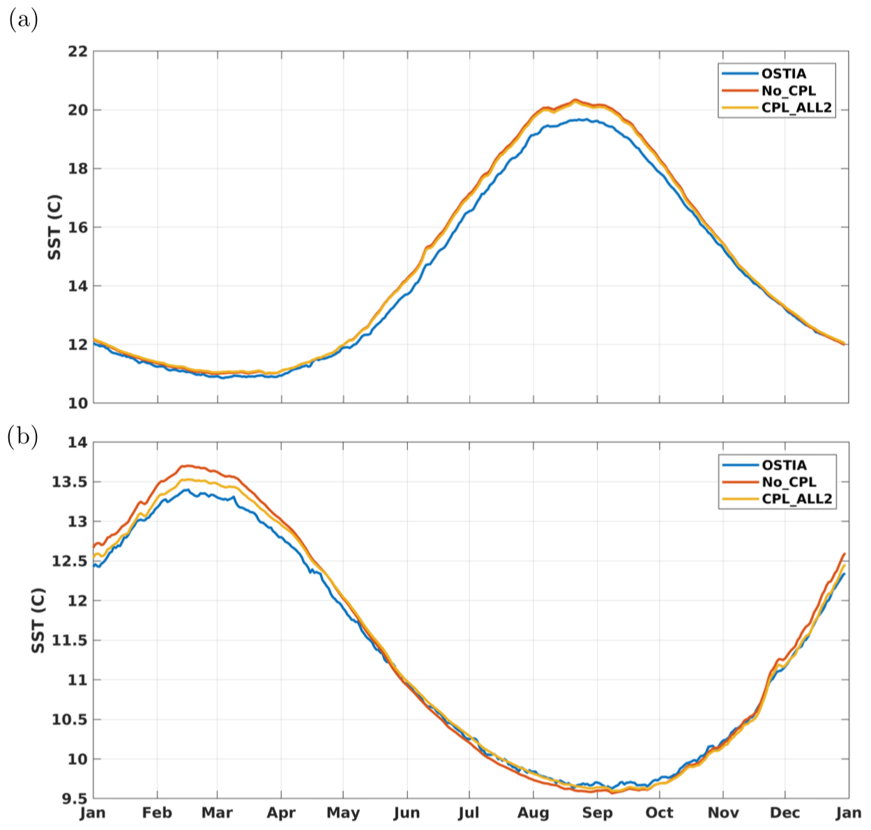
Figure 12Time series of the spatially averaged sea surface temperature (∘C); (a) Northern Hemisphere and (b) Southern Hemisphere.
To better characterize the wave impact on the SST, we show in Fig. 13a the difference in terms of annual mean between the No_CPL experiment and OSTIA analysis, exhibiting a cold bias in the No_CPL simulation in equatorial and tropical regions and a warm bias in the northern part of the Pacific Ocean. The coupling with waves tends to diminish the cold bias (see Fig. 13b), especially in the Pacific Ocean, and the warm bias in the North Pacific is significantly reduced.
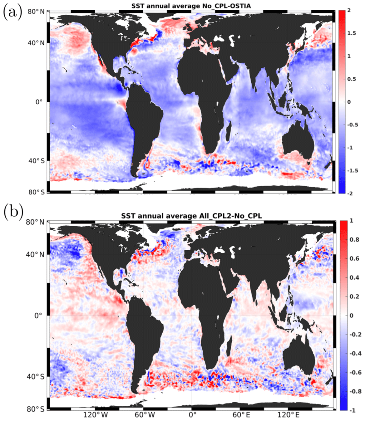
Figure 13(a) Annual average of the differences between No_CPL and OSTIA sea surface temperatures (∘C) for the year 2014 (positive when the model is warmer). (b) Annual average of the difference between All_CPL2 and No_CPL (positive when All_CPL2 is warmer).
As already noticed by Law Chune and Aouf (2018) the warming in the equatorial and tropical regions mainly results from a lower wind stress caused by a value of the Charnock parameter lower than the value used in the uncoupled case (see Fig. 3b, d). A consequence is a decrease in the drag coefficient, leading to smaller turbulent exchange coefficients and reducing the heat flux. As mentioned above, in extratropical regions, some warm bias tends to be partially reduced by the extra mixing induced by the waves at high latitude and/or by the increased turbulent transfer coefficient. The tendency of the wave coupling to improve the near-surface temperature distribution can also be verified on a time–latitude Hovmöller diagram like the ones shown in Fig. 14. For instance, it can be seen that the summer warm bias in the Northern Hemisphere (Fig. 14a) coincides well with the cooling induced by the coupling with waves (Fig. 14b). Similarly we can also observe a warming in the tropical and equatorial regions (Fig. 14b) corresponding to the cold bias seen in Fig. 14a. In the southern extratropical region, a summer cooling is observed. It is induced by the wave coupling, whereas Fig. 14a shows a slight warm bias. During winter we can observe a warming in Fig. 14b north of 60∘ S, which again partially corresponds to a cold bias in Fig. 14a.
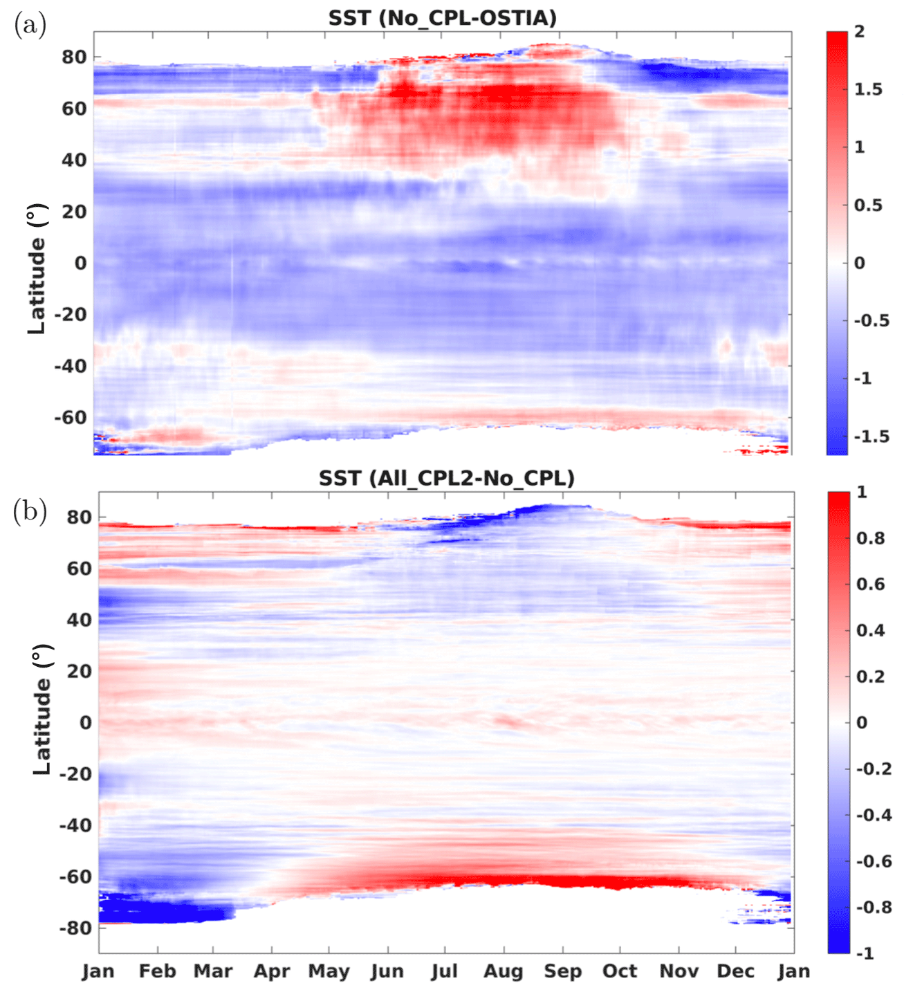
Figure 14Hovmöller diagram of the longitudinally averaged sea surface temperature (∘C) differences between (a) No_CPL and OSTIA and (b) between All_CPL2 and No_CPL.
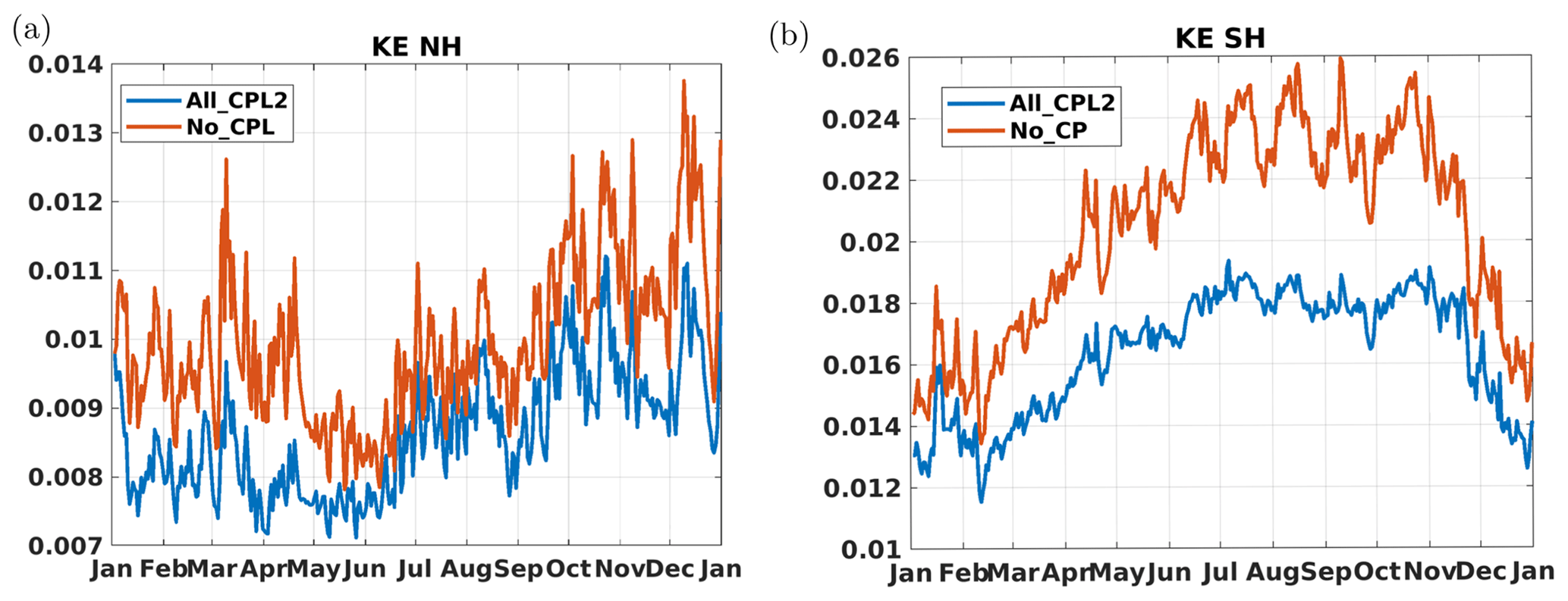
Figure 15Time series of the spatially averaged surface kinetic energy (m2 s−2) for (a) the Northern Hemisphere and (b) the Southern Hemisphere.
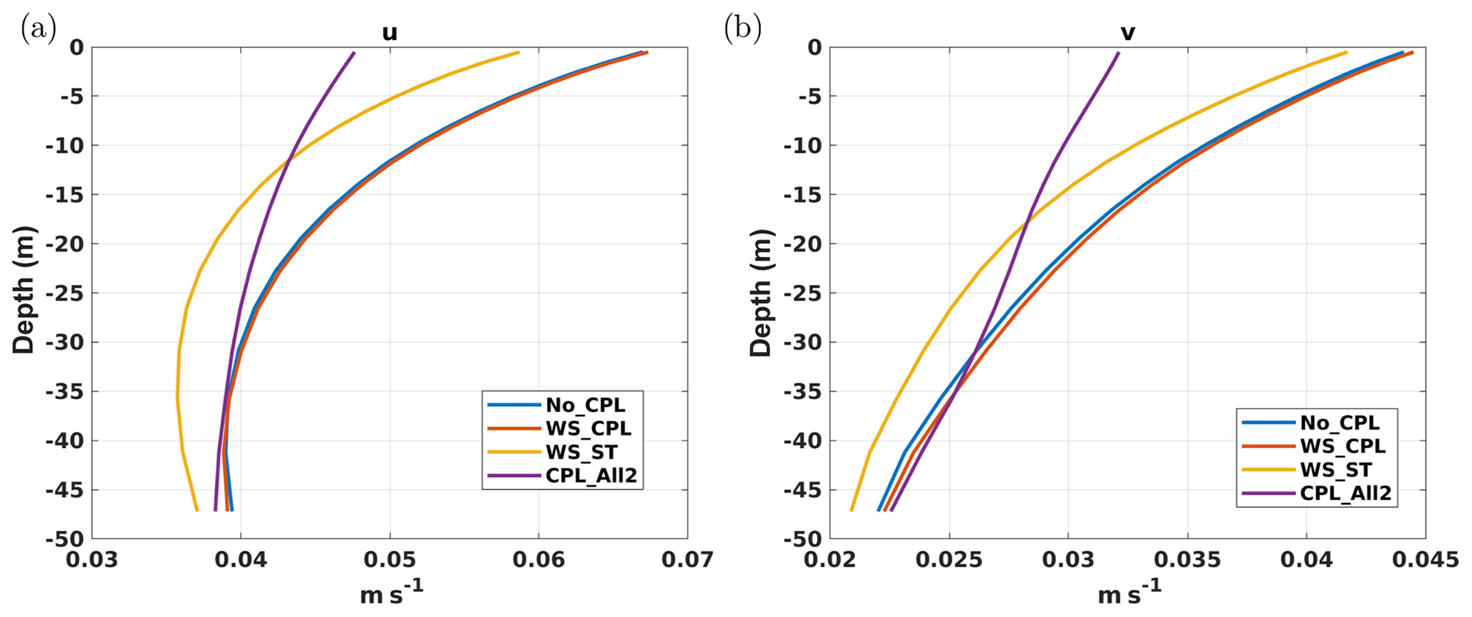
4.2.5 Surface current and kinetic energy
The last aspect of our solutions we would like to evaluate is the impact of the surface waves on surface currents and kinetic energy (KE). To do so, we show in Fig. 15 time series of the spatially averaged surface kinetic energy for both hemispheres. Whatever the hemisphere there is a net decrease in surface KE (up to 20 % in the south) when a coupling with the waves is included. This decrease in surface kinetic energy reflects a decrease in surface current magnitudes. Indeed, as detailed in Fig. 16, which represents the vertical profile of the horizontal components of the current in the oceanic surface boundary layer, the coupling with waves decreases both the surface current magnitudes and the shear. While currents from the WS_CPL are increased due to increased wind stress, the Stokes–Coriolis force when included in momentum equations leads to a decrease in velocities in the whole boundary layer as previously shown by Rascle et al. (2008) (orange lines in Fig. 16). The inclusion of vertical mixing due to waves and Langmuir circulation attenuates the currents in the surface layer, resulting in further reduced surface currents and stronger currents at the bottom of the boundary layer (purple lines in Fig. 16). This concludes our checking of the proper functioning of the coupling with waves as described in the present paper.
In this paper we have described the implementation of an online coupling between the oceanic model NEMO and the wave model WW3. The impact of such coupling on the model solutions has been assessed from the oceanic point of view for a global configuration. In particular, the following steps to set up the coupled model have been discussed in detail: (i) the inclusion of all wave-induced terms in NEMO primitive equations, only neglecting the terms relevant for the surf zone, which is outside the scope of the NEMO community; (ii) modification of the subgrid-scale vertical physics (including the bulk formulation) to include wave effects and a parameterization of Langmuir turbulence; (iii) development of a coupling interface based on the OASIS-MCT software for the exchange of data between the two models; and (iv) tests of our developments on a realistic global configuration at for the ocean coupled to a resolution wave model. Compared to an ocean-only simulation, the coupling with a wave model (with a resolution twice as coarse as the oceanic model) leads to an additional computational cost of about 20 %.
Following McWilliams et al. (2004) and Ardhuin et al. (2008), in the weak vertical current shear limit, the wave-induced terms implemented in NEMO include the Stokes–Coriolis force, the vortex force, Stokes advection in tracer and continuity equations, and a wave-induced surface pressure term. The prognostic equation for TKE also includes an additional forcing term associated with the Stokes drift vertical shear and various modifications of its boundary condition described in Sect. 2.3.
The development of a coupling infrastructure based on OASIS-MCT has several advantages as it allows for an efficient data exchange (including the treatment of nonconformities between the computational grids) but also for versatility in the inclusion of a wave model in existing ocean–atmosphere or ocean-only models. At a practical level, the OASIS interface we have implemented in NEMO is similar to other interfaces (e.g., toward atmospheric models) existing in the code, which is important for maintenance and for further developments. It paves the way for a seamless and more systematic inclusion of the coupling with waves for NEMO users. Unlike most previous studies of wave–ocean coupling using NEMO, we have shown that satisfactory results can be obtained from the TKE vertical turbulent closure scheme without activating the ad hoc parameterization for the mixing induced by near-inertial waves, surface waves, and swell (known as the ETAU parameterization). This parameterization that allows users to empirically propagate the surface TKE at depth using a prescribed shape function is a pragmatic way to cure the shallow mixed layer depths in the Southern Ocean found in simulations ignoring wave effects. Previous studies of wave–ocean coupling by Breivik et al. (2015), Alari et al. (2016), and Staneva et al. (2017) have used the ETAU parameterization in their setup. However, as suggested by Breivik et al. (2015), we can speculate that such a parameterization could mask the impact of the wave coupling even though it turned out to be necessary to obtain realistic mixed layer depths. We believe that our modification of the standard NEMO one-equation TKE scheme described in Sect. 2.3 is more physically justifiable than the ETAU parameterization and requires much less parameter tuning.
The numerical experiments based on the ORCA25 configuration discussed in Sect. 4.2 were meant to check that our developments were having the expected impact on numerical solutions. First, we confirmed that using the Charnock parameter computed in the wave model instead of a constant value globally increases the wind stress magnitude, particularly at middle and high latitudes, whereas accounting for the portion of the wind stress consumed by the waves has a small impact (in our experiments it leads to a maximum 2 % decrease in the wind stress). Second, using the mixed layer depth as an indicator to assess the amount of vertical mixing, the modifications brought to the NEMO turbulence scheme (i.e., the new boundary condition for TKE and for the mixing length, the addition of the Stokes shear in the TKE equation, and the modified Axell (2002) parameterization for Langmuir cells) lead to an important extra mixing contributing to a deepening of the surface mixed layer, particularly in the Southern Hemisphere. When compared to ARGO data it shows a significant improvement during the summer, while during the winter the extra wave-induced mixing deepens the already too deep mixed layer. Note that the Fox-Kemper et al. (2008) parameterization to account for the restratification induced by mixed layer instabilities (Boccaletti et al., 2007; Couvelard et al., 2015) during the winter was not used in our experiments. This parameterization induces even more shallow summer mixed layer depths. As far as the Northern Hemisphere is concerned, coupled results show an improvement when compared to ARGO for winter with a deepening of the mixed layer, while in summer results are similar to the uncoupled case. Since the comparison with ARGO data can be tricky due to the scarcity of data, we looked at the results in terms of mixed layer depth (MLD) probability density functions. This allowed us to highlight the significant improvement in MLD distribution when coupling with the waves. Furthermore, we noticed that all components of the ocean–wave coupling act to deepen the mixed layer and therefore have a cumulative effect. However, the main contributor is the fully modified TKE scheme including the Langmuir cell parameterization of Axell (2002), which is consistent with recent results obtained by Reichl et al. (2016) and Ali et al. (2019) using a K-profile parameterization (KPP) closure scheme.
Since the magnitude of the vertical mixing is increased by the coupling with waves we expect an impact on sea surface temperature and currents. Indeed, the summer deepening of the mixed layer in the Southern Hemisphere leads to colder sea surface temperatures, resulting in better agreement with the OSTIA SST analysis. More generally, although the global SST biases are not totally compensated for, they tend to be reduced when considering the effect of waves (see Sect. 4.2.4). The currents in the oceanic surface boundary layer are reduced by the Stokes–Coriolis force (which counteracts the Ekman current; Rascle et al., 2008). They are also affected by the increased vertical mixing, which tends to reduce the surface currents (and thus the surface kinetic energy) and strengthen the currents at the base of the surface boundary layer. The reduction of surface kinetic energy due to the wave–ocean coupling in the global resolution configuration is of the same order of magnitude as the reduction observed when accounting for surface currents in the computation of the wind stress in a coupled ocean–atmosphere model (e.g., Renault et al., 2016). A fully coupled ocean–wave–atmosphere model would thus be necessary to properly disentangle the different contributions at play impacting the oceanic surface kinetic energy. Even if additional diagnostics on various configurations at different resolutions are still needed to exhaustively evaluate the impact of each component of the ocean wave coupling, the results presented in the paper confirm the robustness of our developments, and our implementation will serve as a starting point for the inclusion of wave–current interactions in the forthcoming NEMO official release. We can speculate that the ocean–wave coupled ORCA025 configuration might become a standard component of future Coupled Model Intercomparison Project (CMIP) exercises. We already mentioned as a perspective the addition of a coupling with an interactive atmospheric boundary layer either via a full atmospheric model or a simplified boundary layer model (e.g., Lemarié et al., 2020). Furthermore, the gain of an online two-way coupling compared to a one-way coupling on the oceanic and wave solution must be investigated in the future. Indeed, the improvements of the quality of surface wave simulations associated with a coupling with large-scale oceanic currents are well documented, particularly in the Agulhas current (Irvine and Tilley, 1988) and in the Gulf Stream (Mapp et al., 1985). Ardhuin et al. (2017a) have also shown a strong impact of small-scale currents (10–100 km) on wave height variability at the same scales. We can therefore expect improvements for both wave and ocean forecasts when the coupling is implemented in an operational context.
In this Appendix we describe the necessary changes when a flux formulation for advective terms in the momentum equations is preferred to the vector-invariant form presented in Eqs. (7) and (8). For simplicity, we consider just the i component in horizontal curvilinear coordinates and the z coordinate in the vertical (results will be extended to the j component and to a generalized vertical coordinate). Consistently with the notations of Madec (2012), e1 and e2 are the horizontal scale factors. We denote the extra term needed to guarantee equivalence between the flux formulation and the vector-invariant form. is defined such that
Since , we have and thus
Hence,
The same computation for the j component leads to the following equations in generalized vertical coordinates.
Here, and are derivatives along the z coordinate.
Single-column experiments based on Noh et al. (2016) have been performed to study the behavior of the NEMO vertical closure with the Langmuir cell parameterization of Axell (2002). In the Noh et al. (2016) experiments the initial condition is given by
with α the thermal expansion coefficient in the equation of state defined as with ρ0=1024 kg m−3. A zonal wind is imposed with m s−1, and the Stokes drift is given by
The various parameter values are
with 96 vertical levels for the discretization and 16 h simulations. We only consider the case with a=1 m and λ=40 m, which gives a turbulent Langmuir number of Lat≈0.32. Numerical results are shown in Fig. B1 (upper panels) and are consistent with the results of Noh et al. (2016) with a deepening of the oceanic mixing length of about 10 m when Langmuir turbulence is accounted for (see LES results in Fig. 3 in Noh et al., 2016). For CLC=0.15 in the Axell (2002) parameterization, the deepening is too weak, while for CLC=0.3 it is closer to the Noh et al. (2016) LES results. Note that for those experiments, the value of dLC is almost identical to the mixed layer depth. Figure B1 (lower panels) illustrates the fact that for a stronger stratification (i.e., with s−2 instead of s−2) the effect of Langmuir turbulence on mixed layer depth is negligible. Indeed, in this case Langmuir cells do not provide enough mixing to erode the stratification.
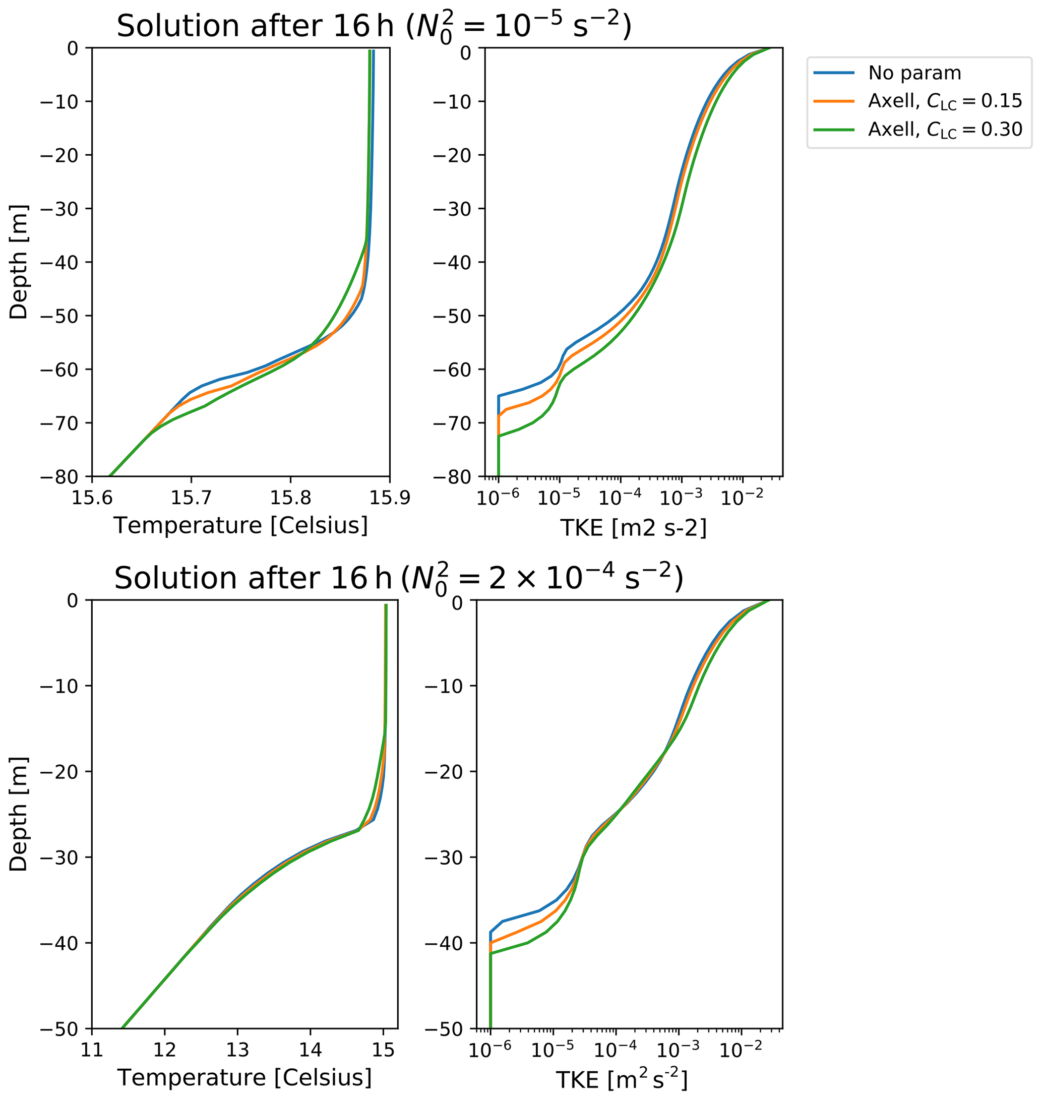
Figure B1Solution obtained for the Noh et al. (2016) single-column experiment after 16 h for different parameter values in the Axell (2002) Langmuir cell parameterization in the case s−2 (upper panels) and s−2 (lower panels).
The changes to the NEMO code have been made on the standard NEMO code (nemo_v3_6_STABLE). The code can be downloaded from the NEMO website (http://www.nemo-ocean.eu/, last access: 11 July 2019, Madec, 2012). The NEMO code modified to include wave–ocean coupling terms and the OASIS interface is available in the Zenodo archive (https://doi.org/10.5281/zenodo.3331463, Couvelard, 2019). The WW3 code version 6.02 has been used without further modifications and can be downloaded from the NOAA GitHub repository (https://github.com/NOAA-EMC/WW3, last access: 11 July 2019, WAVEWATCH III® Development Group, 2016). Our modifications of the OASIS interface in the WW3 code have already been integrated in the official release. The OASIS3_MCT code is also freely available (https://portal.enes.org/oasis/, last access: 11 July 2019, Valcke, 2013; Craig et al., 2017). The exact versions of the WW3 and OASIS3_MCT codes that were used have also been made available in the Zenodo archive (https://doi.org/10.5281/zenodo.3331463, Couvelard, 2019) The initial and forcing data for both the oceanic and wave model, analysis scripts, namelists, and the data used to produce the figures are also available in the Zenodo archive.
XC prepared and carried out all the numerical experiments, investigated the results, and wrote the paper with the help of all the coauthors. GM, FL, RB, and XC made the changes in the NEMO code to include the wave–ocean interactions. GS helped to prepare the necessary datasets for the numerical experiments and analyze the model outputs. FA and JR helped to investigate the results and to formalize the necessary wave-induced terms in both the primitive equations and the TKE closure.
The authors declare that they have no conflict of interest.
We thank George Nurser and Oyvind Breivik, whose efforts helped to improve earlier versions of this paper, as well as Qiang Wang and Svenja Langer. We also thank Knut Klingbeil, Patrick Marchesiello, and Patrick Marsaleix for useful discussions. Xavier Couvelard, Florian Lemarié, and Jean-Luc Redelsperger acknowledge support by Mercator-Ocean and the Copernicus Marine Environment Monitoring Service (CMEMS) through contract 22-GLO-HR – Lot 2 (High-resolution ocean, waves, atmosphere interaction). Numerical simulations were performed on Ifremer HPC facilities DATARMOR of “P∘le de Calcul Intensif pour la Mer” (PCIM) (http://www.ifremer.fr/pcim, last access: 2 July 2020). Mixed layer depth data were graciously provided by Clément de Boyer Montégut, and SST data were downloaded from the CMEMS catalog. The authors also gratefully thank Claude Talandier for help with NEMO, Mickaël Accensi for help with WW3, and Eric Maisonnave and Laure Coquart for their help with OASIS3_MCT.
This paper was edited by Qiang Wang and reviewed by A. J. George Nurser and Oyvind Breivik.
Alari, V., Staneva, J., Breivik, Ø., Bidlot, J.-R., Mogensen, K., and Janssen, P.: Surface wave effects on water temperature in the Baltic Sea: simulation with the coupled NEMO-WAM model, Ocean Dynam., 66, 917–930, https://doi.org/10.1007/s10236-016-0963-x, 2016. a, b, c
Ali, A., Christensen, K. H., Øyvind Breivik, Malila, M., Raj, R. P., Bertino, L., Chassignet, E. P., and Bakhoday-Paskyabi, M.: A comparison of Langmuir turbulence parameterizations and key wave effects in a numerical model of the North Atlantic and Arctic Oceans, Ocean Model., 137, 76–97, https://doi.org/10.1016/j.ocemod.2019.02.005, 2019. a
Arakawa, A. and Lamb, V. R.: A Potential Enstrophy and Energy Conserving Scheme for the Shallow Water Equations, Mon. Weather Rev., 109, 18–36, https://doi.org/10.1175/1520-0493(1981)109<0018:APEAEC>2.0.CO;2, 1981. a
Ardhuin, F. and Jenkins, A. D.: On the interaction of surface waves and upper ocean turbulence, J. Phys. Oceanogr., 36, 551–557, https://doi.org/10.1175/JPO2862.1, 2006. a
Ardhuin, F., Herbers, T. H. C., Watts, K. P., van Vledder, G. P., Jensen, R., and Graber, H. C.: Swell and Slanting-Fetch Effects on Wind Wave Growth, J. Phys. Oceanogr., 37, 908–931, https://doi.org/10.1175/JPO3039.1, 2007. a
Ardhuin, F., Rascle, N., and Belibassakis, K.: Explicit wave-averaged primitive equations using a generalized Lagrangian mean, Ocean Model., 20, 35–60, https://doi.org/10.1016/j.ocemod.2007.07.001, 2008. a, b, c, d, e, f, g
Ardhuin, F., Marié, L., Rascle, N., Forget, P., and Roland, A.: Observation and estimation of Lagrangian, Stokes and Eulerian currents induced by wind and waves at the sea surface, J. Phys. Oceanogr., 39, 2820–2838, https://doi.org/10.1175/2009JPO4169.1, 2009. a
Ardhuin, F., Rogers, E., Babanin, A., Filipot, J.-F., Magne, R., Roland, A., van der Westhuysen, A., Queffeulou, P., Lefevre, J.-M., Aouf, L., and Collard, F.: Semi-empirical dissipation source functions for wind-wave models: part I, definition, calibration and validation, J. Phys. Oceanogr., 40, 1917–1941, https://doi.org/10.1175/2010JPO4324.1, 2010a. a
Ardhuin, F., Rogers, E., Babanin, A. V., Filipot, J.-F., Magne, R., Roland, A., van der Westhuysen, A., Queffeulou, P., Lefevre, J.-M., Aouf, L., and Collard, F.: Semiempirical Dissipation Source Functions for Ocean Waves. Part I: Definition, Calibration, and Validation, J. Phys. Oceanogr., 40, 1917–1941, https://doi.org/10.1175/2010JPO4324.1, 2010b. a, b
Ardhuin, F., Rascle, N., Chapron, B., Gula, J., Molemaker, J., Gille, S. T., Menemenlis, D., and Rocha, C.: Small scale currents have large effects on wind wave heights, J. Geophys. Res., 122, 4500–4517, https://doi.org/10.1002/2016JC012413, 2017a. a
Ardhuin, F., Suzuki, N., McWilliams, J. C., and Aiki, H.: Comments on “A Combined Derivation of the Integrated and Vertically Resolved, Coupled Wave–Current Equations”, J. Phys. Oceanogr., 47, 2377–2385, https://doi.org/10.1175/JPO-D-17-0065.1, 2017b. a
Axell, L. B.: Wind-driven internal waves and Langmuir circulations in a numerical ocean model of the southern Baltic Sea, J. Geophys. Res., 107, 25–1–25–20, https://doi.org/10.1029/2001JC000922, 2002. a, b, c, d, e, f, g, h, i
Banner, M. L. and Morison, R. P.: Refined source terms in wind wave models with explicit wave breaking prediction. Part I: Model framework and validation against field data, Ocean Model., 33, 177–189, https://doi.org/10.1016/j.ocemod.2010.01.002, 2010. a
Banner, M. L. and Young, I. R.: Modeling Spectral Dissipation in the Evolution of Wind Waves. Part I: Assessment of Existing Model Performance, J. Phys. Oceanogr., 24, 1550–1571, https://doi.org/10.1175/1520-0485(1994)024<1550:MSDITE>2.0.CO;2, 1994. a
Barnier, B., Madec, G., Penduff, T., Molines, J.-M., Treguier, A.-M., Le Sommer, J., Beckmann, A., Biastoch, A., Böning, C., Dengg, J., Derval, C., Durand, E., Gulev, S., Remy, E., Talandier, C., Theetten, S., Maltrud, M., McClean, J., and De Cuevas, B.: Impact of partial steps and momentum advection schemes in a global ocean circulation model at eddy-permitting resolution, Ocean Dynam., 56, 543–567, https://doi.org/10.1007/s10236-006-0082-1, 2006. a
Belcher, S. E., Grant, A. L. M., Hanley, K. E., Fox-Kemper, B., Van Roekel, L., Sullivan, P. P., Large, W. G., Brown, A., Hines, A., Calvert, D., Rutgersson, A., Pettersson, H., Bidlot, J.-R., Janssen, P. A. E. M., and Polton, J. A.: A global perspective on Langmuir turbulence in the ocean surface boundary layer, Geophys. Res. Lett., 39, L18605, https://doi.org/10.1029/2012GL052932, 2012. a
Bennis, A.-C., Ardhuin, F., and Dumas, F.: On the coupling of wave and three-dimensional circulation models: Choice of theoretical framework, practical implementation and adiabatic tests, Ocean Model., 40, 260–272, https://doi.org/10.1016/j.ocemod.2011.09.003, 2011. a, b, c
Boccaletti, G., Ferrari, R., and Fox-Kemper, B.: Mixed Layer Instabilities and Restratification, J. Phys. Oceanogr., 37, 2228–2250, https://doi.org/10.1175/JPO3101.1, 2007. a
Boutin, G., Lique, C., Ardhuin, F., Accensi, M., Rousset, C., Talandier, C., and Girard-Ardhuin, F.: Coupling a spectral wave model with a coupled ocean-ice model, Drakkar meeting, Grenoble, France, 21–23 January, available at: http://pp.ige-grenoble.fr/pageperso/barnierb/WEBDRAKKAR2019/ (last access: 2 July 2020), 2019. a
Breivik, Ø., Janssen, P., and Bidlot, J.-R.: Approximate Stokes Drift Profiles in Deep Water, J. Phys. Oceanogr., 44, 2433–2445, 2014. a, b, c
Breivik, Ø., Mogensen, K., Bidlot, J.-R., Balmaseda, M. A., and Janssen, P.: Surface Wave Effects in the NEMO Ocean Model: Forced and Coupled Experiments, J. Geophys. Res.-Oceans, 120, 2973–2992, https://doi.org/10.1002/2014JC010565, 2015. a, b, c, d, e
Breivik, Ø., Bidlot, J.-R., and Janssen, P.: A Stokes drift approximation based on the Phillips spectrum, Ocean Model., 100, 49–56, https://doi.org/10.1016/j.ocemod.2016.01.005, 2016. a, b, c, d
Brodeau, L., Barnier, B., Gulev, S. K., and Woods, C.: Climatologically significant effects of some approximations in the bulk parameterizations of turbulent air-sea fluxes, J. Phys. Oceanogr., 47, 5–28, https://doi.org/10.1175/JPO-D-16-0169.1, 2016. a, b, c
Charnock, H.: Wind stress on a water surface, Q. J. Roy. Meteor. Soc., 81, 639–640, https://doi.org/10.1002/qj.49708135027, 1955. a
Chen, G. and Belcher, S. E.: Effects of Long Waves on Wind-Generated Waves, J. Phys. Oceanogr., 30, 2246–2256, 2000. a
Chen, S. and Curnic, M.: Ocean surface waves in Hurricane Ike (2008) and Superstorm Sandy (2012): Coupled model predictions and observations, Oceanogr. Meteorol., 103, 161–176, https://doi.org/10.5670/oceanog.2010.05, 2015. a
Couvelard, X.: ORCA025-WW3-Couvelard_etal_GMD, https://doi.org/10.5281/zenodo.3331463, 2019. a, b
Couvelard, X., Dumas, F., Garnier, V., Ponte, A., Talandier, C., and Treguier, A.: Mixed layer formation and restratification in presence of mesoscale and submesoscale turbulence, Ocean Model., 96, 243–253, https://doi.org/10.1016/j.ocemod.2015.10.004, 2015. a
Craig, A., Valcke, S., and Coquart, L.: Development and performance of a new version of the OASIS coupler, OASIS3-MCT_3.0, Geosci. Model Dev., 10, 3297–3308, https://doi.org/10.5194/gmd-10-3297-2017, 2017. a, b, c
Craig, P. D. and Banner, M. L.: Modeling Wave-Enhanced Turbulence in the Ocean Surface Layer, J. Phys. Oceanogr., 24, 2546–2559, 1994. a
D'Asaro, E. A., Thomson, J., Shcherbina, A. Y., Harcourt, R. R., Cronin, M. F., Hemer, M. A., and Fox-Kemper, B.: Quantifying upper ocean turbulence driven by surface waves, Geophys. Res. Lett., 41, 102–107, https://doi.org/10.1002/2013GL058193, 2014. a
Deardorff, J. W.: Stratocumulus-capped mixing layers derived from a threedimensional model, Bound.-Lay. Meteorol., 18, 495–527, 1980. a
de Boyer Montégut, C., Madec, G., Fischer, A. S., Lazar, A., and Iudicone, D.: Mixed layer depth over the global ocean: An examination of profile data and a profile-based climatology, J. Geophys. Res., 109, C12003, https://doi.org/10.1029/2004JC002378, 2004. a, b
Dee, D. P., Uppala, S. M., Simmons, A. J., Berrisford, P., Poli, P., Kobayashi, S., Andrae, U., Balmaseda, M. A., Balsamo, G., Bauer, P., Bechtold, P., Beljaars, A. C. M., van de Berg, L., Bidlot, J., Bormann, N., Delsol, C., Dragani, R., Fuentes, M., Geer, A. J., Haimberger, L., Healy, S. B., Hersbach, H., Hólm, E. V., Isaksen, L., Kållberg, P., Köhler, M., Matricardi, M., McNally, A. P., Monge-Sanz, B. M., Morcrette, J.-J., Park, B.-K., Peubey, C., de Rosnay, P., Tavolato, C., Thépaut, J.-N., and Vitart, F.: The ERA-Interim reanalysis: configuration and performance of the data assimilation system, Q. J. Roy. Meteor. Soc., 137, 553–597, https://doi.org/10.1002/qj.828, 2011. a
Ducousso, N., Le Sommer, J., Molines, J.-M., and Bell, M.: Impact of the “ymmetric Instability of the Computational Kind” at mesoscale- and submesoscale-permitting resolutions, Ocean Model., 120, 18–26, https://doi.org/10.1016/j.ocemod.2017.10.006, 2017. a
Fairall, C. W., Bradley, E. F., Hare, J. E., Grachev, A. A., and Edson, J. B.: Bulk Parameterization of Air–Sea Fluxes: Updates and Verification for the COARE Algorithm, J. Climate, 16, 571–591, https://doi.org/10.1175/1520-0442(2003)016<0571:BPOASF>2.0.CO;2, 2003. a
Fan, Y. and Griffies, S. M.: Impacts of Parameterized Langmuir Turbulence and Nonbreaking Wave Mixing in Global Climate Simulations, J. Climate, 27, 4752–4775, https://doi.org/10.1175/JCLI-D-13-00583.1, 2014. a
Fox-Kemper, B., Ferrari, R., and Hallberg, R.: Parameterization of Mixed Layer Eddies. Part I: Theory and Diagnosis, J. Phys. Oceanogr., 38, 1145–1165, https://doi.org/10.1175/2007JPO3792.1, 2008. a
Hasselmann, K.: Ocean circulation and climate change, Tellus B, 43, 82–103, https://doi.org/10.3402/tellusb.v43i4.15399, 1991. a
Hasselmann, S., Hasselmann, K., Allender, H., and Barnet, T. P.: Computations and parameterizations of the nonlinear energy transfer in a gravity wave spectrum. Part II. Parameterizations of the nonlinear energy transfer for application in wave models , J. Phys. Oceanogr., 15, 1378–1391, 1985. a
Hilburn, K.: The passive microwave water cycle product, Remote Sensing Systems (REMSS) Technical Report 072409, Santa Rosa (CA), 30 pp., Tech. rep., 2009. a
Hwang, P. A.: Fetch- and Duration-Limited Nature of Surface Wave Growth inside Tropical Cyclones: With Applications to Air–Sea Exchange and Remote Sensing*, J. Phys. Oceanogr., 46, 41–56, 2015. a
Irvine, D. E. and Tilley, D. G.: Ocean wave directional spectra and wave-current interaction in the Agulhas from the Shuttle Imaging Radar-B synthetic aperture radar, J. Geophys. Res.-Oceans, 93, 15389–15401, https://doi.org/10.1029/JC093iC12p15389, 1988. a
Jacob, R., Larson, J., and Ong, E.: M × N Communication and Parallel Interpolation in Community Climate System Model Version 3 Using the Model Coupling Toolkit, Int. J. High Perform. C., 19, 293–307, https://doi.org/10.1177/1094342005056116, 2005. a
Janssen, P. A.: Progress in ocean wave forecasting, J. Comp. Phys., 227, 3572–3594, https://doi.org/10.1016/j.jcp.2007.04.029, 2008. a
Janssen, P. A. E. M.: Quasi-linear Theory of Wind-Wave Generation Applied to Wave Forecasting, J. Phys. Oceanogr., 21, 1631–1642, 1991. a
Janssen, P. A. E. M.: On some consequences of the canonical transformation in the Hamiltonian theory of water waves, J. Fluid Mech., 637, 1–44, https://doi.org/10.1017/S0022112009008131, 2009. a
Komen, G. J., Cavaleri, L., Donelan, M., Hasselmann, K., Hasselmann, S., and Janssen, P. A. E. M.: Dynamics and modelling of ocean waves, Cambridge University Press, Cambridge, 1994. a
Large, W. G. and Yeager, S. G.: The global climatology of an interannually varying air–sea flux data set, Clim. Dynam., 33, 341–364, https://doi.org/10.1007/s00382-008-0441-3, 2009. a
Law Chune, S. and Aouf, L.: Wave effects in global ocean modeling: parametrizations vs. forcing from a wave model, Ocean Dynam., 68, 1739–1758, https://doi.org/10.1007/s10236-018-1220-2, 2018. a, b, c, d
Leclair, M. and Madec, G.: A conservative leap-frog time stepping method, Oceanogr. Meteorol., 30, 88–94, https://doi.org/10.1016/j.ocemod.2009.06.006, 2009. a
Lemarié, F., Samson, G., Redelsperger, J.-L., Giordani, H., Brivoal, T., Masson, S., and Madec, G.: A simplified atmospheric boundary layer model for an improved representation of air-sea interactions in eddying oceanic models: implementation and first evaluation in NEMO(4.0), Geosci. Model Dev. Discuss., submitted, 2020. a
Li, Q., Webb, A., Fox-Kemper, B., Craig, A., and Danabasoglu, G.: Langmuir mixing effects on global climate: WAVEWATCH III in CESM, Oceanogr. Meteorol., 103, 145–160, https://doi.org/10.1016/j.ocemod.2015.07.020, 2016. a
Li, Q., Fox-Kemper, B., Breivik, O., and Webb, A.: Statistical models of global Langmuir mixing, Oceanogr. Meteorol., 113, 95–114, https://doi.org/10.1016/j.ocemod.2017.03.016, 2017. a, b
Lévy, M., Estublier, A., and Madec, G.: Choice of an advection scheme for biogeochemical models, Geophys. Res. Lett., 28, 3725–3728, https://doi.org/10.1029/2001GL012947, 2001. a
Madec, G.: NEMO ocean engine, in: Note du Pole de modélisation No. 27, Institut Pierre-Simon Laplace (IPSL), France, 2012. a, b, c, d, e, f, g
Mapp, G. R., Welch, C. S., and Munday, J. C.: Wave refraction by warm core rings, J. Geophys. Res.-Oceans, 90, 7153–7162, https://doi.org/10.1029/JC090iC04p07153, 1985. a
McWilliams, J. C., Restrepo, J. M., and Lane, E. M.: An asymptotic theory for the interaction of waves and currents in coastal waters, J. Fluid Mech., 511, 135–178, https://doi.org/10.1017/S0022112004009358, 2004. a, b, c
Mellor, G. and Blumberg, A.: Wave breaking and ocean surface layer thermal response, J. Phys. Oceanogr., 34, 693–698, 2004. a, b
Michaud, H., Marsaleix, P., Leredde, Y., Estournel, C., Bourrin, F., Lyard, F., Mayet, C., and Ardhuin, F.: Three-dimensional modelling of wave-induced current from the surf zone to the inner shelf, Ocean Sci., 8, 657–681, https://doi.org/10.5194/os-8-657-2012, 2012. a
Moghimi, S., Klingbeil, K., Gräwe, U., and Burchard, H.: A direct comparison of a depth-dependent Radiation stress formulation and a Vortex force formulation within a three-dimensional coastal ocean model, Ocean Model., 70, 132–144, https://doi.org/10.1016/j.ocemod.2012.10.002, 2013. a
Noh, Y., Ok, H., Lee, E., Toyoda, T., and Hirose, N.: Parameterization of Langmuir Circulation in the Ocean Mixed Layer Model Using LES and Its Application to the OGCM, J. Phys. Oceanogr., 46, 57–78, 2016. a, b, c, d, e, f, g
Phillips, O.: On the response of short ocean wave components at fixed wavenumber to ocean current variations, J. Phys. Oceanogr., 14, 1425–1433, 1984. a
Polonichko, V.: Generation of Langmuir circulation for nonaligned wind stress and the Stokes drift, J. Geophys. Res., 102, 15773–15780, https://doi.org/10.1029/97JC00460, 1997. a, b
Rascle, N. and Ardhuin, F.: Drift and mixing under the ocean surface revisited: Stratified conditions and model-data comparisons, J. Geophys. Res., 114, C02016, https://doi.org/10.1029/2007JC004466, 2009. a
Rascle, N. and Ardhuin, F.: A global wave parameter database for geophysical applications. Part 2: model validation with improved source term parameterization, Ocean Modelling, 70, 174–188, https://doi.org/10.1016/j.ocemod.2012.12.001, 2013. a, b
Rascle, N., Ardhuin, F., Queffeulou, P., and Croizé-Fillon, D.: A global wave parameter database for geophysical applications. Part 1: wave-current-turbulence interaction parameters for the open ocean based on traditional parameterizations, Ocean Model., 25, 154–171, https://doi.org/10.1016/j.ocemod.2008.07.006, 2008. a, b, c
Redelsperger, J. L., Mahé, F., and Carlotti, P.: A Simple And General Subgrid Model Suitable Both For Surface Layer And Free-Stream Turbulence, Bound.-Lay. Meteorol., 101, 375–408, 2001. a
Reichl, B. G., Ginis, I., Hara, T., Thomas, B., Kukulka, T., and Wang, D.: Impact of Sea-State-Dependent Langmuir Turbulence on the Ocean Response to a Tropical Cyclone, Mon. Weather Rev., 144, 4569–4590, https://doi.org/10.1175/MWR-D-16-0074.1, 2016. a
Renault, L., Molemaker, M. J., McWilliams, J. C., Shchepetkin, A. F., Lemarié, F., Chelton, D., Illig, S., and Hall, A.: Modulation of Wind Work by Oceanic Current Interaction with the Atmosphere, J. Phys. Oceanogr., 46, 1685–1704, https://doi.org/10.1175/JPO-D-15-0232.1, 2016. a, b
Rodgers, K. B., Aumont, O., Mikaloff Fletcher, S. E., Plancherel, Y., Bopp, L., de Boyer Montégut, C., Iudicone, D., Keeling, R. F., Madec, G., and Wanninkhof, R.: Strong sensitivity of Southern Ocean carbon uptake and nutrient cycling to wind stirring, Biogeosciences, 11, 4077–4098, https://doi.org/10.5194/bg-11-4077-2014, 2014. a, b
Roquet, F., Madec, G., McDougall, T., and Barker, P.: An accurate polynomial expression for the TEOS-10 equation of state for use in ocean general circulation models., Oceanogr. Meteorol., 90, 29–43, https://doi.org/10.1016/j.ocemod.2015.04.002, 2015. a, b
Rousset, C., Vancoppenolle, M., Madec, G., Fichefet, T., Flavoni, S., Barthélemy, A., Benshila, R., Chanut, J., Levy, C., Masson, S., and Vivier, F.: The Louvain-La-Neuve sea ice model LIM3.6: global and regional capabilities, Geosci. Model Dev., 8, 2991–3005, https://doi.org/10.5194/gmd-8-2991-2015, 2015. a
Skyllingstad, E. D. and Denbo, D. W.: An ocean large-eddy simulation of Langmuir circulations and convection in the surface mixed layer, J. Geophys. Res., 100, 8501–8522, https://doi.org/10.1029/94JC03202, 1995. a
Staneva, J., Alari, V., Breivik, Ø., Bidlot, J.-R., and Mogensen, K.: Effects of wave-induced forcing on a circulation model of the North Sea, Ocean Dynam., 67, 81–101, 2017. a, b
Stopa, J. E., Sutherland, P., and Ardhuin, F.: Strong and highly variable push of ocean waves on Southern Ocean sea ice, P. Natl. Acad. Sci. USA, 115, 5861–5865, https://doi.org/10.1073/pnas.1802011115, 2018. a
Suzuki, N. and Fox-Kemper, B.: Understanding Stokes forces in the wave-averaged equations, J. Geophys. Res., 121, 3579–3596, https://doi.org/10.1002/2015JC011566, 2016. a, b
Tennekes, H. and Lumley, J. L.: A first course in turbulence, The MIT Press, 1972. a
Tolman, H. L., Balasubramaniyan, B., Burroughs, L. D., Chalikov, D. V., Chao, Y. Y., Chen, H. S., and Gerald, V. M.: Development and Implementation of Wind-Generated Ocean Surface Wave Modelsat NCEP, Weather Forecast., 17, 311–333, https://doi.org/10.1175/1520-0434(2002)017<0311:DAIOWG>2.0.CO;2, 2002. a
Uchiyama, Y., McWilliams, J. C., and Shchepetkin, A. F.: Wave–current interaction in an oceanic circulation model with a vortex-force formalism: Application to the surf zone, Ocean Model., 34, 16–35, https://doi.org/10.1016/j.ocemod.2010.04.002, 2010. a
UNESCO: Algorithms for computation of fundamental property of sea water, 44, 1983. a
Valcke, S.: The OASIS3 coupler: a European climate modelling community software, Geosci. Model Dev., 6, 373–388, https://doi.org/10.5194/gmd-6-373-2013, 2013. a, b, c
Van Roekel, L. P., Fox-Kemper, B., Sullivan, P. P., Hamlington, P. E., and Haney, S. R.: The form and orientation of Langmuir cells for misaligned winds and waves, J. Geophys. Res., 117, C05001, https://doi.org/10.1029/2011JC007516, 2012. a, b
WAVEWATCH III® Development Group: User manual and system documentation of WAVEWATCH III ® version 5.16, Tech. Note 329, NOAA/NWS/NCEP/MMAB, College Park, MD, USA, 326 pp. + Appendices, 2016. a, b, c
Wu, L., Staneva, J., Breivik, O., Rutgersson, A., Nurser, A. G., Clementi, E., and Madec, G.: Wave effects on coastal upwelling and water level, Ocean Model., 140, 101405, https://doi.org/10.1016/j.ocemod.2019.101405, 2019. a, b
In the notations of Ardhuin et al. (2008) this term corresponds to .
In the notations of Ardhuin et al. (2008) this term corresponds to .
In Mellor and Blumberg (2004) the authors consider a Dirichlet boundary condition such that and an equivalent Neumann condition . The authors claim that numerical solutions using a Dirichlet condition instead of a Neumann condition are qualitatively similar.
- Abstract
- Introduction
- Inclusion of wave-induced terms in the oceanic model NEMO
- Modeling system and coupling strategy
- Global coupled wave–ocean simulations
- Conclusions
- Appendix A: Flux-form wave-averaged momentum equations
- Appendix B: Sensitivity to the cLC parameter from single-column experiments
- Code and data availability
- Author contributions
- Competing interests
- Acknowledgements
- Review statement
- References