IPSL-CM5A2 – an Earth system model designed for multi-millennial climate simulations

Based on the fifth phase of the Coupled Model Intercomparison Project (CMIP5)-generation previous Institut Pierre Simon Laplace (IPSL) Earth system model, we designed a new version, IPSL-CM5A2, aiming at running multi-millennial simulations typical of deep-time paleoclimate studies. Three priorities were followed during the setup of the model: (1) improving the overall model computing performance, (2) overcoming a persistent cold bias depicted in the previous model generation and (3) making the model able to handle the specific continental configurations of the geological past. These developments include the integration of hybrid parallelization Message Passing Interface – Open Multi-Processing (MPI-OpenMP) in the atmospheric model of the Laboratoire de Météorologie Dynamique (LMDZ), the use of a new library to perform parallel asynchronous input/output by using computing cores as “I/O servers” and the use of a parallel coupling library between the ocean and the atmospheric components. The model, which runs with an atmospheric resolution of $\mathrm{3.75}{}^{\circ }\times \mathrm{1.875}{}^{\circ }$ and 2 to 0.5^∘ in the ocean, can now simulate ∼100 years per day, opening new possibilities towards the production of multi-millennial simulations with a full Earth system model. The tuning strategy employed to overcome a persistent cold bias is detailed. The confrontation of a historical simulation to climatological observations shows overall improved ocean meridional overturning circulation, marine productivity and latitudinal position of zonal wind patterns. We also present the numerous steps required to run IPSL-CM5A2 for deep-time paleoclimates through a preliminary case study for the Cretaceous. Namely, specific work on the ocean model grid was required to run the model for specific continental configurations in which continents are relocated according to past paleogeographic reconstructions. By briefly discussing the spin-up of such a simulation, we elaborate on the requirements and challenges awaiting paleoclimate modeling in the next years, namely finding the best trade-off between the level of description of the processes and the computing cost on supercomputers.

1 Introduction

Despite the rise of high-performance computing (HPC; all acronyms except model names are defined in Appendix D), the ever-growing complexity and resolution of general circulation models (and subsequent Earth system models; ESMs) have restricted their use to centennial integrations for future climate projections, or short “snapshot” experiments for paleoclimates, with durations ranging from decades to a few thousand years. Longer simulations of several thousand years are yet often desirable. Millennial-length simulations are useful to project very long-term future climatic trends but also to properly quantify equilibrium climate sensitivity of models (Rugenstein et al., 2020). In paleoclimate studies, such long simulations are mandatory to either (i) reach a fully equilibrated deep ocean when initialized from idealized thermohaline conditions (a typical procedure in deep-time, pre-Quaternary – i.e., older than 2.6-million-year paleoclimate simulations) or (ii) address multi-millennial transient climate evolution such as glacial–interglacial cycles of the Quaternary period (He, 2011). Through the years, several strategies have been set up to overcome the issue of the computing cost of long integrations. They involve both the development of dedicated models and peculiar experimental designs. Regarding the former, different models have been used:

• Earth system models of intermediate complexity (Claussen et al., 2002), with coarse spatial resolution and simplifications in the physics, allow very efficient computation times and have been used extensively to explore Quaternary paleoclimates and run transient simulations (Roberts et al., 2014; Caley et al., 2014). As an example, the iLOVECLIM model (Goosse et al., 2010; Roche, 2013) provides more than 2500 simulated years per day (hereafter SYPD) on one computing core at a ∼5.6^∘ spatial resolution (three vertical levels) in the atmosphere and a full ocean general circulation model (OGCM) at $\mathrm{3}{}^{\circ }\times \mathrm{3}{}^{\circ }$ (21 vertical levels) with two tracers. Performance is still 850 SYPD with 20 tracers in the ocean (Bouttes et al., 2015b; Missiaen et al., 2020).

• Versions of fully coupled general circulation models (GCMs) have been maintained at very low (∼5–7^∘) spatial resolutions, allowing long integrations in a reasonable amount of wall-clock time. Examples include FOAM (Fast Ocean Atmosphere Model). It couples the National Center for Atmospheric Research (NCAR) Community Climate Model version 2 (CCM2) ($\mathrm{7.5}{}^{\circ }\times \mathrm{4.5}{}^{\circ }$ and 18 vertical levels but an updated physics equivalent to the NCAR CCM3 model) atmosphere model and an ocean model similar to Geophysical Fluid Dynamics Laboratory (GFDL) Modular Ocean Model (MOM). It reaches an average of 250 SYPD and has been routinely used for almost 20 years in numerous deep-time paleoclimate studies (Brown et al., 2009; Donnadieu et al., 2006; Ladant et al., 2014; Pohl et al., 2014; Poulsen et al., 2001; Roberts et al., 2014). FAMOUS (FAst Met Office/UK Universities Simulator), as part of the BRIDGE HadCM3 family of climate models (Valdes et al., 2017), is another example. It runs at a 7.5^∘ longitude × 5^∘ latitude resolution with 11 levels in the atmosphere and averages 450 SYPD, and that is frequently used for paleoclimate (e.g., Gregoire et al., 2012; Roberts et al., 2014 and future climate studies (Bouttes et al., 2015a).

• Climate modeling groups have also maintained versions of their GCMs at a low (∼2–4^∘) resolution. Within the BRIDGE HadCM3 family, HadCM3BL ($\mathrm{3.75}{}^{\circ }\times \mathrm{2.5}{}^{\circ }$ and 19 levels in the atmosphere; $\mathrm{3.75}{}^{\circ }\times \mathrm{2.5}{}^{\circ }$ and 20 vertical levels in the ocean) is used to perform long integrations at 85 SYPD (e.g., Kennedy-Asser et al., 2020). NCAR has also developed a low-resolution (T31 – i.e., approximately 3.75^∘ longitude × 3.75^∘ latitude, 26 vertical levels, 35 SYPD) version of the CCSM3 GCM (Yeager et al., 2006) that provided “the first synchronously coupled atmosphere–ocean general circulation model simulation from the Last Glacial Maximum to the Bølling-Allerød (BA) warming” (Roberts et al., 2014) as well as transient Holocene simulations (Liu et al., 2014). CCSM3 has been used also to run a transient simulation of the last deglaciation within the TraCE program (He, 2011). NCAR has released a similar version for CCSM4 (Shields et al., 2012), at the same “low resolution”, with performance reaching 64 SYPD. This model has been used for multi-millennial fully coupled paleoclimate simulations (Brierley and Fedorov, 2016; Burls et al., 2017). A similar strategy has been applied with the ECHAM5/MPI-OM model (formerly known as COSMOS), which has been used at T31 resolution in the atmosphere for long paleoclimate simulations of the Holocene (Dallmeyer et al., 2017; Fischer and Jungclaus, 2011) and has been recently implemented with water isotopes (Werner et al., 2016).

  Experimental designs dedicated to multi-millennial simulations have also followed different strategies through the years:

• Early methods to circumvent the constraint of computation time have involved (i) using atmospheric-only models forced by prescribed sea-surface temperatures (e.g., Roberts et al., 2014), (ii) coupling the atmospheric component to mixed-layer ocean models with prescribed heat transport – i.e., slab ocean models – (Otto-Bliesner and Upchurch, 1997) and (iii) asynchronous coupling between atmospheric and ocean models (Bice et al., 2000). If efficient in terms of computation time, such strategies prevented any assessment of ocean dynamics and associated feedbacks on the climate system. Later, experimental designs with GCMs for deep-time paleoclimate modeling relied on simulations branched on each other (i.e., the final state of equilibrated simulations is used as an initial state for new simulations with a different forcing) to make the ocean reach different equilibria in a reasonable amount of time (namely less than 1000 years; Liu et al., 2009).

• For transient experiments, i.e., with an evolving insolation, Lorenz and Lohmann (2004) proposed an accelerated insolation forcing; when the simulation calendar advances by 1 year, the calendar for the computation of the incoming insolation advances by 10 to 100 years. The method assumes that the fast components of the climate system (atmosphere, upper ocean) are in constant equilibrium with insolation. It is suitable only for periods of time with almost no change for the slow components (deep ocean, land ice). This method is easily implementable in any climate model (e.g., Crosta et al., 2018). This acceleration technique has been used multiple times with CCSM3, the latest example being the study of the last 140 000 years of climate evolution of Africa by Kutzbach et al. (2020). Others have applied a “multiple snapshots” strategy, involving several multi-centennial (200 to 500 years) simulations forced by varying orbital parameters, to explore the impact of insolation on the fast components of the climate system (Singarayer and Valdes, 2010; Marzocchi et al., 2015).

• Statistical approaches based on multiple simulations also allowed to explore transient climate changes. They involve either the use of statistical emulators, calibrated using several steady-state GCM simulations, with varying orbital configurations and atmospheric pCO₂ concentrations (Lord et al., 2017) or linear approximations between single-forcing simulations (Erb et al., 2015; Simon et al., 2017).

The original IPSL-CM5A-LR (IPSL stands for “Institut Pierre Simon Laplace”; we will omit the -LR suffix in the following) model was developed and released in 2013 “to study the long-term response of the climate system to natural and anthropogenic forcings as part of the fifth phase of the Coupled Model Intercomparison Project (CMIP5)” (Dufresne et al., 2013). This Earth system model coupled the Laboratoire de Météorologie Dynamique zoom (LMDZ5) atmospheric model ($\mathrm{3.75}\times \mathrm{1.875}{}^{\circ }$ in longitude–latitude, 39 vertical levels) (Hourdin et al., 2013) and Organising Carbon and Hydrology In Dynamic Ecosystems (ORCHIDEE) land surface model (Krinner et al., 2005) with the Nucleus for European Modelling of the Ocean (NEMO) (Madec, 2015), which includes ocean and sea-ice dynamics (2^∘ resolution and 31 vertical levels in the ocean), together with the marine biogeochemical model PISCES (Aumont et al., 2015). IPSL-CM5A has been used for several paleoclimate studies (e.g., Kageyama et al., 2013; Roberts et al., 2014; Tan et al., 2017; Zhuang and Giardino, 2012), including studies benefiting from the explicit representation of marine biogeochemistry (Bopp et al., 2017; Ladant et al., 2018; Le Mézo et al., 2017), vegetation dynamics and land biosphere (Tan et al., 2017). Still, IPSL-CM5A computation time, which averages 10 SYPD, has hindered its use for multi-millennial experiments that are typical for Quaternary or “deep-time” paleoclimate studies in which a fully equilibrated deep ocean is mandatory. In this paper, we present and evaluate IPSL-CM5A2, a CMIP5-class ESM, including interactive vegetation and carbon cycle and designed for multi-thousand-year experiments.

2 From IPSL-CM5A to IPSL-CM5A2

Apart from better computing performance, setting up IPSL-CM5A2 aimed at reducing two of the main biases of IPSL-CM5A. First, an important cold bias has been depicted in global surface air temperature (t2m) in IPSL-CM5A (Dufresne et al., 2013). This cold bias is associated with a position of the atmospheric eddy driven jets too far equatorward beyond the spread of other CMIP5 models, especially in the northern Pacific and Southern Hemisphere (Barnes and Polvani, 2013). Moreover, the Atlantic Meridional Overturning Circulation (AMOC) has maximum values between 8 and 10 Sv in historical simulations with IPSL-CM5A, a value lower than the observation range and below the values obtained in the other CMIP5 models (Zhang and Wang, 2013).

IPSL-CM5A2 development was initiated in 2017 on the CURIE supercomputer, operated at the Très Grand Centre de Calcul (TGCC), Bruyères-le-Châtel, France, as a part of the GENCI French computing consortium. CURIE offered different fractions of ×86–64 computing resources, including 5040 “thin” nodes (BullX B510). Each node was made of two 8-core 2.7 GHz Intel Sandy Bridge processors, providing a total of 80 640 cores for computation. CURIE was replaced by the JOLIOT-CURIE supercomputer in July 2018. On the latter machine, IPSL models are run on a partition of 1656 nodes, each node made of two 24-core 2.7 GHz Intel Skylake processors, providing a total of 79 488 cores for computation. Here, we depict how IPSL-CM5A2 differs from IPSL-CM5A in terms of components (Sect. 2.1) and technical characteristics (Sect. 2.2). Then we present the computing performance of the new model, first on CURIE compared to IPSL-CM5A as it was originally conducted, then on JOLIOT-CURIE, the TGCC machine that will be used in the next years by the IPSL climate model community and on which we conducted a set of scaling experiments (Sect. A2).

2.1 IPSL-CM5A2 components: evolution from IPSL-CM5A

IPSL-CM5A2 is built on updated versions of IPSL-CM5A components and is configured at the same spatial resolutions, i.e., the regular $\mathrm{3.75}\times \mathrm{1.875}{}^{\circ }$ longitude–latitude grid and 39 vertical levels for LMDZ, and the ORCA2 curvilinear grid for NEMO, which is 2^∘ with a refinement to 0.5^∘ in the tropics, and 31 vertical levels (Fig. 1 and Table 1). This choice results from an early evaluation of the performance presented in Appendix A. Here, we target the significant differences between the two models and provide a brief summary of each component. We refer the reader to Dufresne et al. (2013) for a more detailed description of LMDZ, NEMO and ORCHIDEE characteristics.

Table 1 Characteristics of IPSL-CM5 and IPSL-CM5A2 models components.

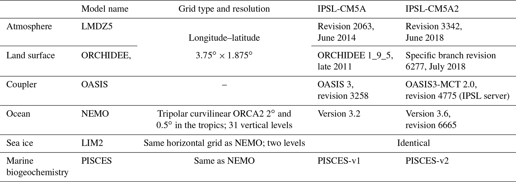
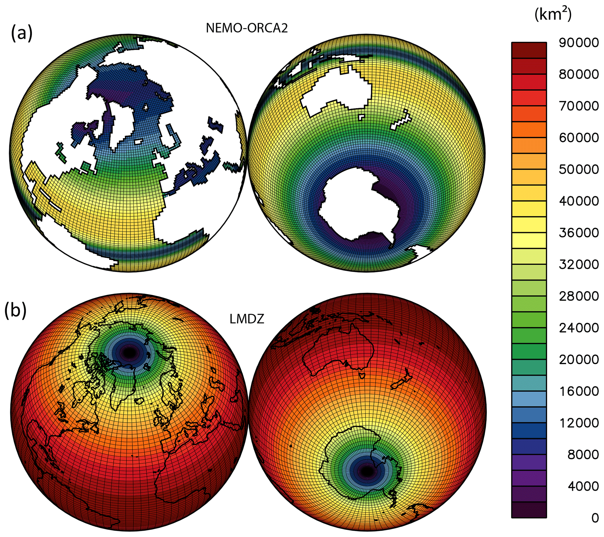
Figure 1 NEMO (a) and LMDZ (b) grid cell areas, in km², showing the refinements of the ocean grid in the tropics and over the Mediterranean Sea as well as the refinement of the atmospheric grid to the pole.

2.1.1 LMDZ

LMDZ is the atmospheric general circulation model developed at Laboratoire de Météorologie Dynamique, France. LMD models have been the atmospheric component of the IPSL coupled models since the earliest IPSL coupled model, which included LMD5.3 (Braconnot et al., 1997). LMDZ is based on the coupling of a dynamical core in which primitive equations of meteorology are discretized and a set of physical parameterizations is created. Here, we use the version LMDZ5A, where A designates the so-called “standard physics” (SP) for the physical atmospheric parameterizations, also used in IPSL-CM5A. The choice of keeping these CMIP5-like physical settings and not benefiting from improvements in the representation of convective boundary layer, cumulus clouds and the diurnal cycle of continental convective rainfall included in the “new physics” (NP) is driven both by (i) the fact that no coupled version of the IPSL model including the new parameterizations was available when the IPSL-CM5A2 project was initialized and (ii) computing cost. The NP parameterizations in LMDZ have been validated for higher vertical resolution (79 levels) and require higher-frequency time coupling between the physics and the dynamics. SP indeed requires a time step for the dynamics of 3 min and a coupling every 30 min with the physics, whereas dynamics is computed every 2.15 min and coupled every 15 min in NP, leading to significant increase in computation time (see the next section). In terms of revision nomenclature, IPSL-CM5A included LMDZ5, revision 2063, whereas IPSL-CM5A2 includes revision 3342. This represents a >2-year gap between both versions. The differences mainly concern bug fixes and various improvements in the physical–dynamic interface in preparation for the next generation of models. They have very limited effect on model results and translate into a slight improvement in energy conservation.

2.1.2 ORCHIDEE

ORCHIDEE (Krinner et al., 2005) is a dynamic global vegetation model (DGVM) that can run either in stand-alone mode, coupled to LMDZ, or included as the land surface component in the IPSL climate model. ORCHIDEE is made of three parts: (i) the “hydrology module” SECHIBA (Schématisation des Echanges Hydriques à l'Interface entre la Biosphère et l'Atmosphère) (de Rosnay and Polcher, 1998; Ducoudré et al., 1993), (ii) parameterizations regarding vegetation dynamics based on plant functional types (PFTs) and derived from the Lund–Potsdam–Jena (LPJ) DGVM (Sitch et al., 2003) and (iii) a “carbon module” called STOMATE (Saclay Toulouse Orsay Model for the Analysis of Terrestrial Ecosystems) that simulates vegetation phenology and carbon dynamics. SECHIBA “describes exchanges of energy and water between the atmosphere and the biosphere, and the soil water budget” (Krinner et al., 2005) with a time step of 30 min. In IPSL-CM5A and IPSL-CM5A2, SECHIBA includes a two-layer soil hydrology scheme, in which maximum water storage capacity is set globally to 300 kg m⁻² over a 2 m soil depth (Guimberteau et al., 2014). Water is redistributed between the two layers through a downward flux parameterized following the early ideas of Choisnel (Choisnel et al., 1995; Ducharne et al., 1998). Rain falling from the canopy feeds the upper layer that loses water both by root extraction and soil evaporation, whereas water storage in the bottom layer decreases only as a function root extraction (Guimberteau et al., 2014). When total soil moisture storage reaches the maximum water storage, the excess water amount is converted to runoff. STOMATE links the fast hydrologic and biophysical processes to the slow processes of vegetation dynamics from LPJ. It includes formulations for photosynthesis, carbon allocation, leaf phenology and respiration (autotrophic and heterotrophic). Vegetation is represented through 13 PFTs, one including bare soil. Each PFT is characterized by specific parameters controlling their dynamics, i.e., climatic control of vegetation establishment, elimination, light competition, fire occurrence and tree mortality. IPSL-CM5A2 includes the version 3930 of the ORCHIDEE model, whereas IPSL-CM5A was based on an older tagged version (ORCHIDEE 1_9_5, for the record). From the technical point of view, these two versions differ in that the IPSL-CM5A2 version of ORCHIDEE benefits from the XML-IO-SERVER (XIOS) for output diagnostics and from hybrid (Message Passing Interface – Open Multi-Processing; MPI-OpenMP) parallelization, as for LMDZ. Amongst several bug corrections, continental evaporation computation has been corrected to ensure a full closure of the water budget.

2.1.3 NEMO-LIM2-PISCES

NEMO has been upgraded from v3.2 to v3.6. River runoff is now added through a non-zero depth and has a specific temperature and salinity. Although a new version of the sea-ice model (LIM3; Rousset et al., 2015) has been developed and is included in the sixth version of the IPSL model (IPSL-CM6A, Boucher et al., 2020), the coupling with the ocean model on the ORCA2 mesh was not ready and we chose to keep the LIM2 configuration for IPSL-CM5A2. LIM2 (Fichefet and Maqueda, 1997; Timmermann et al., 2005) is a sea-ice model with a single sea-ice category. Open water is represented through ice concentration. As stated in Uotila et al. (2017), who provide a detailed comparison between LIM2 and LIM3 in the NEMO, LIM2 implements the snow–ice formation by infiltration and freezing of seawater into snow when deep enough. The effect of subgrid-scale snow and ice thickness distributions is implicitly parameterized by enhancing the conduction of heat through the ice and by melting the ice laterally to account for thin ice melting. The surface albedo depends on the state of the surface (frozen or melting), snow depth and ice thickness following Shine and Henderson-Sellers (1985). The biogeochemical component of NEMO is PISCES (Pelagic Interaction Scheme for Carbon and Ecosystem Studies) and has been upgraded from PISCES-v1 (Aumont and Bopp, 2006) in IPSL-CM5A to PISCES-v2 (Aumont et al., 2015) in IPSL-CM5A2. PISCES simulates the ocean carbon cycle and includes a simple representation of the lower trophic-level ecosystem, with four plankton functional types (two for phytoplankton and two for zooplankton) and the cycles of the main oceanic nutrients (N, P, Si, Fe). Without any change for the general model structure (with 24 state variables), the transition from PISCES-v1 to PISCES-v2 does include a number of developments, e.g., on the iron cycle, on zooplankton grazing, on dissolved and particulate organic matter cycling (see Aumont et al., 2015 for a detailed description).

2.2 Technical developments

Technical developments have been performed on both individual components and the coupling system to accelerate the entire coupled model.

2.2.1 OASIS3-MCT coupling library and interpolation scheme for ocean–atmosphere exchanges

The ocean–sea ice–atmosphere coupling is close to the one used in IPSL-CM5A (Dufresne et al., 2013), except the coupling system has been switched from OASIS3.3 to OASIS3-MCT (Model Coupling Toolkit; Valcke, 2013), which constitutes a parallel coupling library used in both NEMO and LMDZ components. It ensures fully parallel interpolation and exchange of the coupling fields. As in IPSL-CM5A, 24 coupling fields are exchanged, 7 from the ocean to the atmosphere and 17 from the atmosphere to the ocean (Valcke, 2013).

2.2.2 XIOS library

The use of XIOS as input/output library allows performing parallel asynchronous input/output by using computing cores as “I/O servers”. These servers are dedicated to the reading and the writing of the data and permit model computation to continue, while data are written or read.

2.2.3 Integration of hybrid parallelization MPI-OpenMP in LMDZ atmospheric component

In LMDZ, longitudinal filtering is applied on the dynamical equations for latitude higher than 60^∘ in both hemispheres (Hourdin et al., 2013). Thus, the choice of MPI domain decomposition is optimal only along latitudinal bands. This decomposition has been initiated in the LMDZ version of IPSL-CM5A with a minimum of three latitude bands per MPI process, reduced to two in IPSL-CM5A2. In addition, the use of multi-core processors in HPC led us to add a shared memory parallel processing (OpenMP) in LMDZ. The use of this shared memory parallelism on vertical levels in the dynamics allows to increase the number of cores used on the supercomputer and consequently to reduce the elapsed time of the simulation (see Appendix A).

3 Tuning IPSL-CM5A2

IPSL-CM5A2 is evaluated through two sets of simulations. First, we describe the setup of a steady-state pre-industrial simulation that involved several experiments with tuning steps and bug fixes. This setup is used to discuss the tuning strategy, the model large-scale characteristics, ocean spin-up, energy and freshwater budgets, as well as multi-centennial ocean variability. Second, a transient “historical” simulation, forced by boundary condition between years 1850 and 2005, has been designed to evaluate the model with respect to observations (Sect. 4).

3.1 Tuning: target and strategy

We focus here on the general tuning strategy adopted by defining the target and how we reached it, rather than giving a comprehensive description of the numerous simulations that have been designed to obtain the final pre-industrial simulation. As depicted in Hourdin et al. (2017), several choices need to be made when tuning a model, namely defining a relevant target and associated metrics, defining in what mode the model is to be tuned (e.g., atmospheric only, fully coupled) and choosing which parameters will be used to reach the target. As most of modeling groups (Hourdin et al., 2017), our choice was to tune IPSL-CM5A2 through pre-industrial runs, using alternatively atmospheric and fully coupled experiments. A first untuned 1000-year spin-up of IPSL-CM5A2 forced by CMIP5 pre-industrial boundary conditions provided an equilibrated global surface air temperature of 11.3 ^∘C. Such a cold bias had been depicted in IPSL-CM5A (Dufresne et al., 2013). We targeted to increase global-mean surface temperature by 2.2 ^∘C to reach 13.5 ^∘C in pre-industrial conditions with IPSL-CM5A2, expecting this value to translate into 14.5 ^∘C for a present-day simulation, a value consistent with observations (Dee et al., 2011).

Regarding the free parameters, the choice was to use a parameter which controls the conversion of cloud water to rainfall to alter the cloud radiative forcing (CRF) and thereby the top-of-atmosphere (TOA) net radiation (Q_TOA, counted positive downward) and the global-mean surface temperature. Using clouds parameters for tuning, the most uncertain parameters that affect the most radiation, is also well shared practice among modeling groups. Previous results obtained with LMDZ and IPSL-CM5A show that changing the TOA balance by 1 W m⁻² results in a change in temperature of 1 ^∘C. It is also the typical value of the sensitivity of global temperature to greenhouse gas concentration. Our +2.2 ^∘C target thus translates into an increase of Q_TOA by 2.2 W m⁻². In LMDZ, the conversion of cloud water to rainfall is computed following Sundqvist (1978) as

$$\begin{array}{}\text{(1)}& {\displaystyle \frac{\mathrm{d}{q}_{\mathrm{lw}}}{\mathrm{d}t}}=-{\displaystyle \frac{q_{\mathrm{lw}}}{{\mathit{\tau }}_{\mathrm{conv}}}}\left[\mathrm{1}-e^{-{\left(\frac{q_{\mathrm{lw}}}{c_{\mathrm{lw}}}\right)}^{\mathrm{2}}}\right],\end{array}$$

where q_lw is the mixing ratio, c_lw is the in-cloud water threshold for autoconversion, set at 0.418 g kg⁻¹ in IPSL-CM5A. For q_lw>>c_lw, the time constant for auto-conversion is τ_conv (here set at 1800 s), while it goes to infinity (no auto-conversion) for q_lw≪c_lw.

Decreasing c_lw is expected to lower cloud water content and reduce the CRF. First, we carried out atmospheric-only simulations with varying c_lw values to define the sensitivity of Q_TOA to c_lw. The resulting linear relationship provided a value of 0.325 g kg⁻¹ for c_lw to obtain an increase of 2.2 W m⁻² in Q_TOA. Thus, we ran a second pre-industrial fully coupled simulation of 500 years with this tuning. This experiment was interrupted when two bugs (the first was an erroneous computation of the weights necessary to exchange fluxes between the ocean and the atmosphere introduced in the IPSL-CM5A2 versions of OASIS and ORCHIDEE, and the second was a water conservation issue in the land surface scheme) were identified and fixed. A second set of tuning was required as the bug correction altered the global 2 m temperature. After several adjustments, the target of +2.2 W m⁻² at TOA was expected to be obtained by setting c_lw at 0.343 g kg⁻¹. An ultimate fully coupled experiment (called PREIND here) including this tuning was then branched on the previous simulation and run for 2800 years.

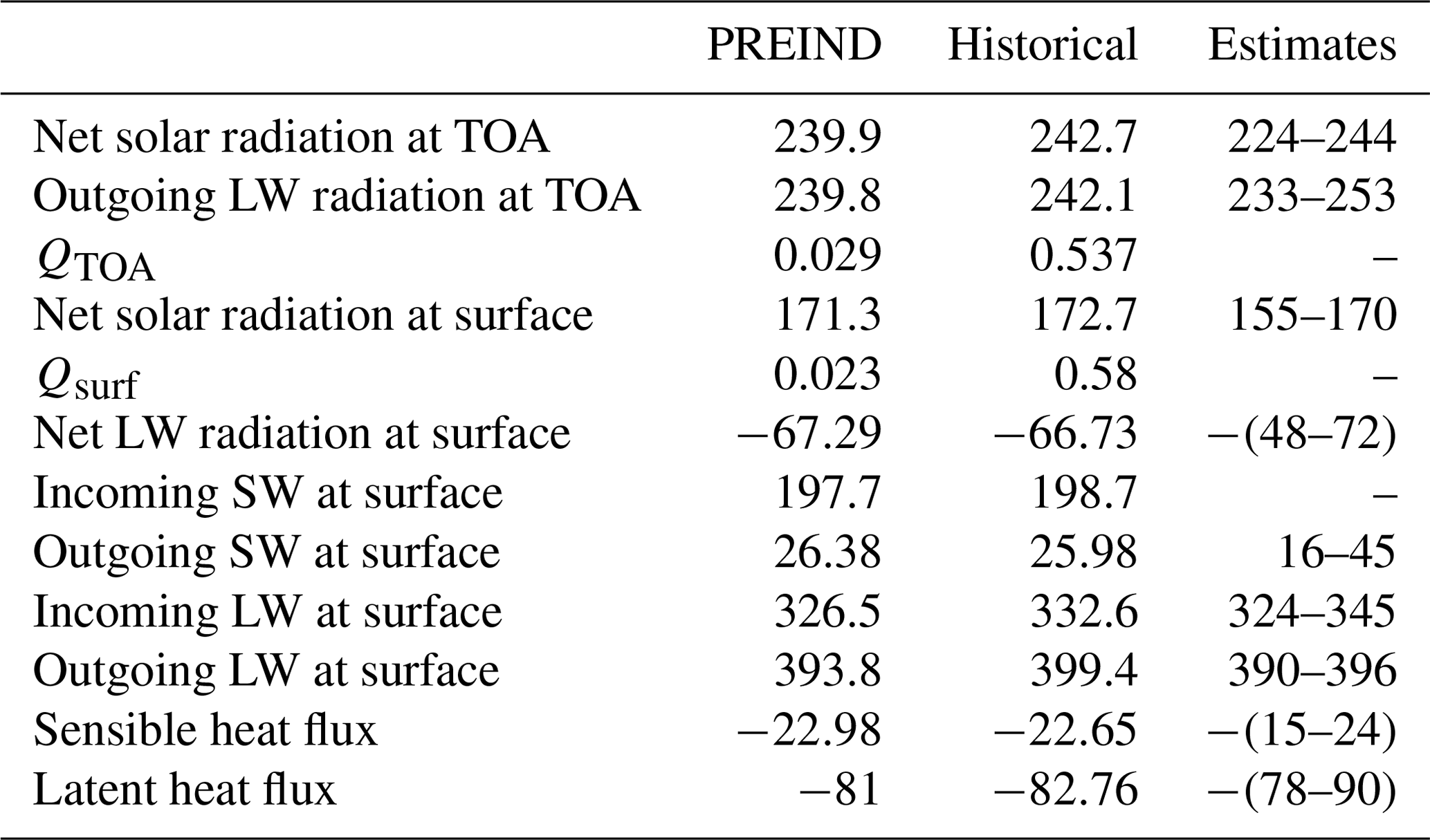
Table 2 Global yearly averages of the radiative budget terms (in W m⁻²) for the last 100 years of PREIND and the historical experiment for the 1980–1999 period. Estimated values come from Trenberth et al. (2009), based on the Earth Radiation Budget Experiment (ERBE) period (1985–1989) or on the CERES period (2000–2004) and retrieved from Voldoire et al. (2013).

3.2 Energetic and freshwater balances, equilibrium and drifts

As expected, the imposed tuning induces a decrease in CRF in our pre-industrial run (−18.97 W m⁻² before tuning, −16.80 W m⁻² after tuning; see Sect. 4.1 for more details about CRF). Table 2 shows the terms of the energetic balance averaged over the last decade of simulation. After 2800 years of integration, pre-industrial Q_TOA and Q_surf are stabilized to values close to zero (respectively, 0.029 and 0.023 W m⁻²), showing an acceptable energetic imbalance and limited spurious energy excess or deficit. Energy conservation is not fully ensured neither in the NEMO nor in the LMDZ component of the model, but the global numerical leak is small. The non-conservative term, expressed as the difference between Q_TOA and the ocean heat content (OHC) change $\frac{\partial \mathrm{OHC}}{\partial t}$ (Hobbs et al., 2016), is small (0.094 W m⁻² over the last 1000 years) compared to IPSL-CM5A (0.18 W m⁻²), which might be an improvement linked to corrections of energy conservation between IPSL-CM5A and IPSL-CM5A2 versions of LMDZ (see Sect. 2.1). Figure 2a indicates that this imbalance is constant after ∼300 years of the pre-industrial simulation, and that OHC stabilizes after ∼2000 years of simulation. This ensures that the model drift is small, therefore validating the use of IPSL-CM5A2 for multi-millennial simulations.

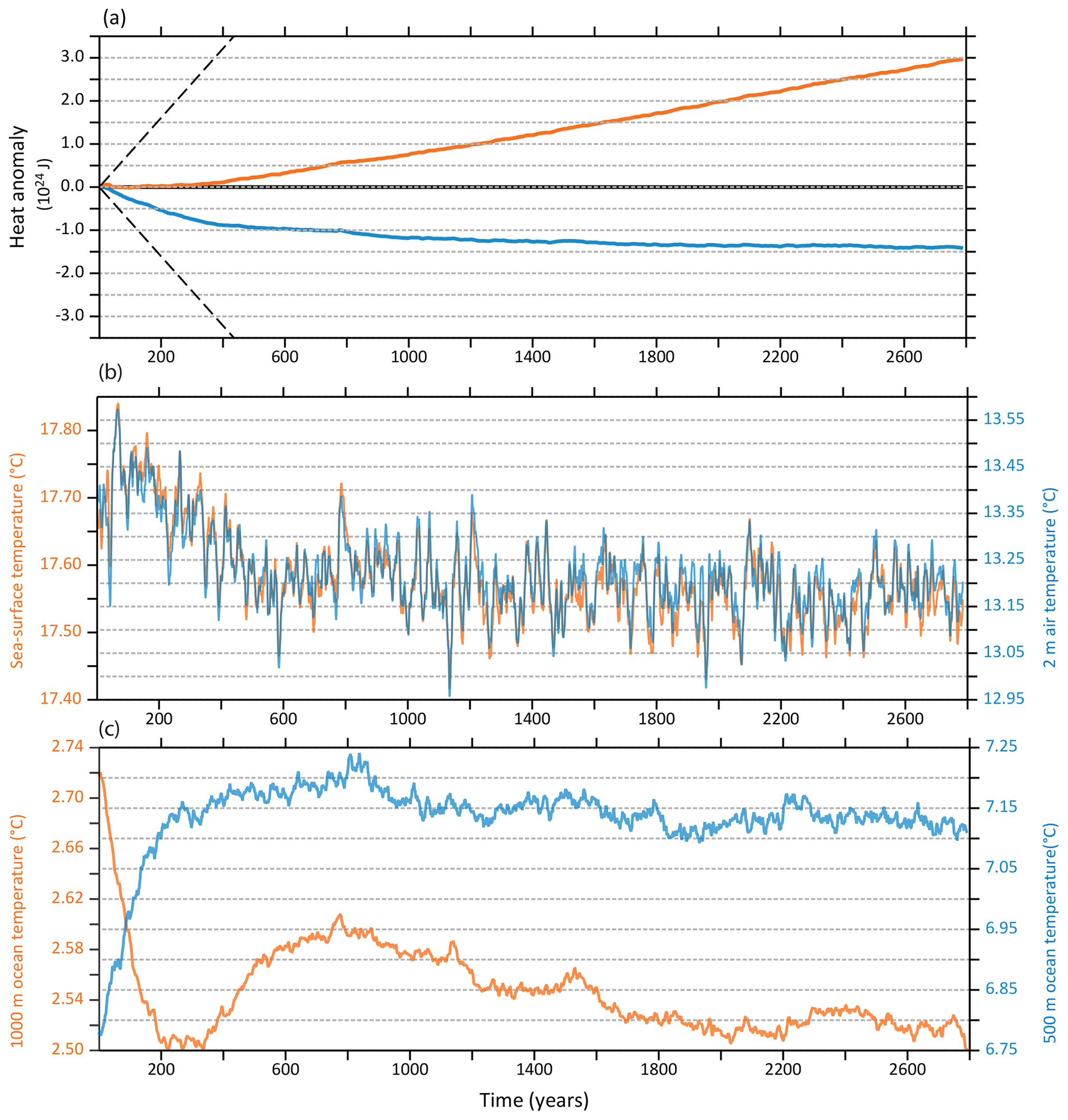
Figure 2 Time series of globally averaged variables over the 2800 years of the PREIND experiment. (a) Annual mean heat content anomaly (10²⁴ J) implied by Q_TOA (orange line, cumulative values) and OHC (blue line). As in Hobbs et al. (2016), dashed black lines show the heat content implied by a Q_TOA of ±0.5 W m⁻², the observed late 20th century Q_TOA (Roemmich et al., 2015). (b) Sea-surface temperature (orange) and 2 m air temperature (blue). (c) 1000 m (orange) and 500 m (blue) ocean potential temperature.

It takes about 500 years for sea-surface temperatures and 2 m air to stabilize after PREIND initialization (Fig. 2b). They converge to 17.5 and 13.2 ^∘C, when globally averaged, respectively. We thus missed the 13.5 ^∘C target by 0.3 ^∘C, which is reasonable when considering the very simple procedure used. Such a difference is also small enough compared to the regional biases in sea-surface temperature. An additional 1500 years are required for the global average ocean temperature to stabilize, as deeper ocean temperatures still cool by ∼0.1 to 0.2 ^∘C during this period (Fig. 2c).

Over the entire PREIND experiment, sea-surface height (SSH) depicts a constant positive drift of 0.19 m per century, revealing that the freshwater budget is not fully closed (not shown). This issue already existed in previous versions of the model and is partly linked to the absence of a proper freshwater conservation between ocean and sea-ice components of NEMO. As a consequence, a linear decrease in global ocean salinity is simulated, corresponding to a steady global ocean freshening of $\mathrm{2}\times {\mathrm{10}}^{-\mathrm{3}}$ psu per century. It appears that this drift varies with global sea-ice volume, as shown by abrupt 4×CO₂ simulations that are characterized by a drift in SSH reduced to 0.01 m per century and a corresponding weaker freshening of the global ocean ($\mathrm{4.7}\times {\mathrm{10}}^{-\mathrm{4}}$ psu per century, not shown). Such a drift might be problematic in the future if IPSL-CM5A2 is to be used for very long (transient-like) integrations. Improvements on this concern are expected from the future replacement of LIM2 by the more recent LIM3 version (Rousset et al., 2015), for which conservation is ensured.

4 Comparison of IPSL-CM5A and IPSL-CM5A2 with observations

A historical experiment was performed starting from the last year of the 2800-year PREIND spin-up. This transient simulation was integrated for 155 years between 1850 and 2005. Boundary conditions are described in Dufresne et al. (2013). Yearly evolution of long-lived greenhouse gases concentrations and total solar irradiance (TSI) correspond to the historical requirements of the CMIP5 project, with notably reduced TSI to consider the volcanic radiative forcing based on an updated version of Sato et al. (1993). Tropospheric aerosols, tropospheric and stratospheric ozone were prepared as described in Szopa et al. (2013) and land use changes processed from crop and pasture datasets developed by Hurtt et al. (2011), as described in Dufresne et al. (2013). Unless otherwise expressed, comparison between the historical run and observations is made by using a mean seasonal cycle for the period of 1980–2005. The comparison between simulated and observed cloud radiative forcing is made using the Clouds and the Earth's Radiant Energy System (CERES) energy balanced and filled fluxes (EBAF) gridded dataset over the period of 2000–2004 (Loeb et al., 2009).

4.1 Atmosphere mean state and identified biases

4.1.1 Cloud radiative forcing

LMDZ5A (and hereby IPSL-CM5A) has been shown to underestimate low and mid-level cloud cover and overestimate high-level clouds at midlatitudes and high latitudes (Hourdin et al., 2013), biases shared with many climate models (Zhang et al., 2005). LMDZ5A cloud representation has been since strongly improved with the new set of physical parameterizations and associated increase in vertical resolution (Hourdin et al., 2020) that is currently being used for CMIP6 project. In IPSL-CM5A2, the biases of the standard parameterization translate into CRF, with too-reflective clouds and therefore too-negative shortwave CRF at midlatitudes and high latitudes (−15 to −25 W m⁻²), and in some convective regions of the tropics an underestimation of outgoing longwave trapping and therefore too-positive LW CRF (+5 to +15 W m⁻²), when compared to the CERES dataset. The tuning depicted earlier leads to a less negative total CRF at all latitudes compared to IPSL-CM5A (Fig. 3).

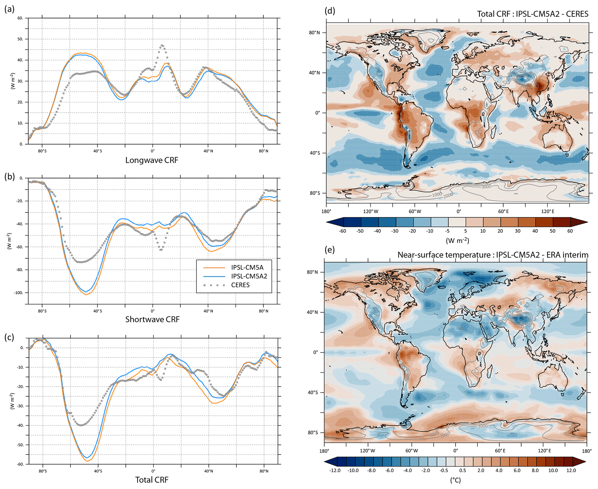
Figure 3 Zonally averaged longwave (a), shortwave (b) and total (c) cloud radiative forcing (in W m⁻²) from IPSL-CM5A2 and IPSL-CM5A historical simulations, compared to the Clouds and the Earth’s Radiant Energy System (CERES) gridded dataset (Loeb et al., 2009). (d) Yearly averaged total CRF anomaly between IPSL-CM5A2 and CERES data. As CRF is a negative value, a positive (negative) anomaly indicates an underestimation (overestimation) of the absolute value of the CRF in the model. (e) Yearly averaged difference in near-surface air temperature (^∘C) between IPSL-CM5A2 and ERA-Interim (Dee et al., 2011). Grey contours indicate surface elevation.

The too-negative CRF in the Southern Hemisphere midlatitudes is only slightly corrected, as less negative shortwave (SW) CRF and is partly compensated by less positive longwave (LW) CRF (Fig. 3a, b, c). In the southern tropics, the tuning mostly worsens the model biases in SW and LW CRF, in relation to a feedback loop in the continental tropical areas (namely the Amazon), where convection is reduced. Tuning still improves total CRF between 15 and 40^∘ N, driven by the better estimation of SW CRF over the oceans. The positive bias of CRF over the eastern boundaries of Atlantic and Pacific oceans remains unchanged (Fig. 3d) and is partly related to a bad representation of low clouds over these regions (Hourdin et al., 2015). These biases translate into surface air temperature biases (Fig. 3e). Regions with positive bias of CRF (e.g., the eastern boundaries of the Pacific and the south Atlantic) are associated with up to 2.5 ^∘C warm biases. Conversely, regions with negative bias of CRF, like the northern and southern Atlantic and several mountain ranges (the Andes, the Rockies and the Tibetan Plateau), show cold biases (down to −6 ^∘C for the Tibetan Plateau).

4.1.2 Temperature and general circulation

The tuning of IPSL-CM5A2 induces a low-latitude warming whose amplitude varies with height, from +1 ^∘C at 850 hPa to +2.5 ^∘C at 200 hPa, when compared to IPSL-CM5A, as expected from the adjustment of the moist adiabatic lapse rate (Fig. 4a). As a consequence of the increased the latitudinal temperature gradient between 200 and 300 hPa, the zonal jets expand towards high latitudes, especially in the Northern Hemisphere (Fig. 4b). This is an improvement, as IPSL-CM5A had been shown to underestimate the jets' latitudinal extension (Barnes and Polvani, 2013). Despite this improvement, IPSL-CM5A2 still underestimates the jet extension in the Southern Hemisphere, as shown by a negative anomaly in zonal wind in the high latitudes and an overestimation of the zonal winds in the low latitudes. At 850 hPa and the surface, IPSL-CM5A2 provides a better representation of the zonal winds in the high latitudes: the negative anomaly with ERA-Interim is reduced along the Antarctic, showing that the westerlies have moved southward. The 850 hPa temperature anomalies also show that tuning has been effective in IPSL-CM5A2 to reduce the cold bias of the model but also that the warm bias over the eastern tropical Pacific has strengthened. In the tropics, IPSL-CM5A2 depicts biases similar to IPSL-CM5A; i.e., over the Pacific Ocean, the surface easterlies' bad seasonal cycle led to an overall yearly misposition, in relation to the double Intertropical Convergence Zone (ITCZ), and over the Atlantic, easterlies' strength is systematically underestimated (not shown). IPSL-CM5A2 also shows overestimated winter westerlies in the northern midlatitudes that translate into an anomalous wind stress over the northern Atlantic.

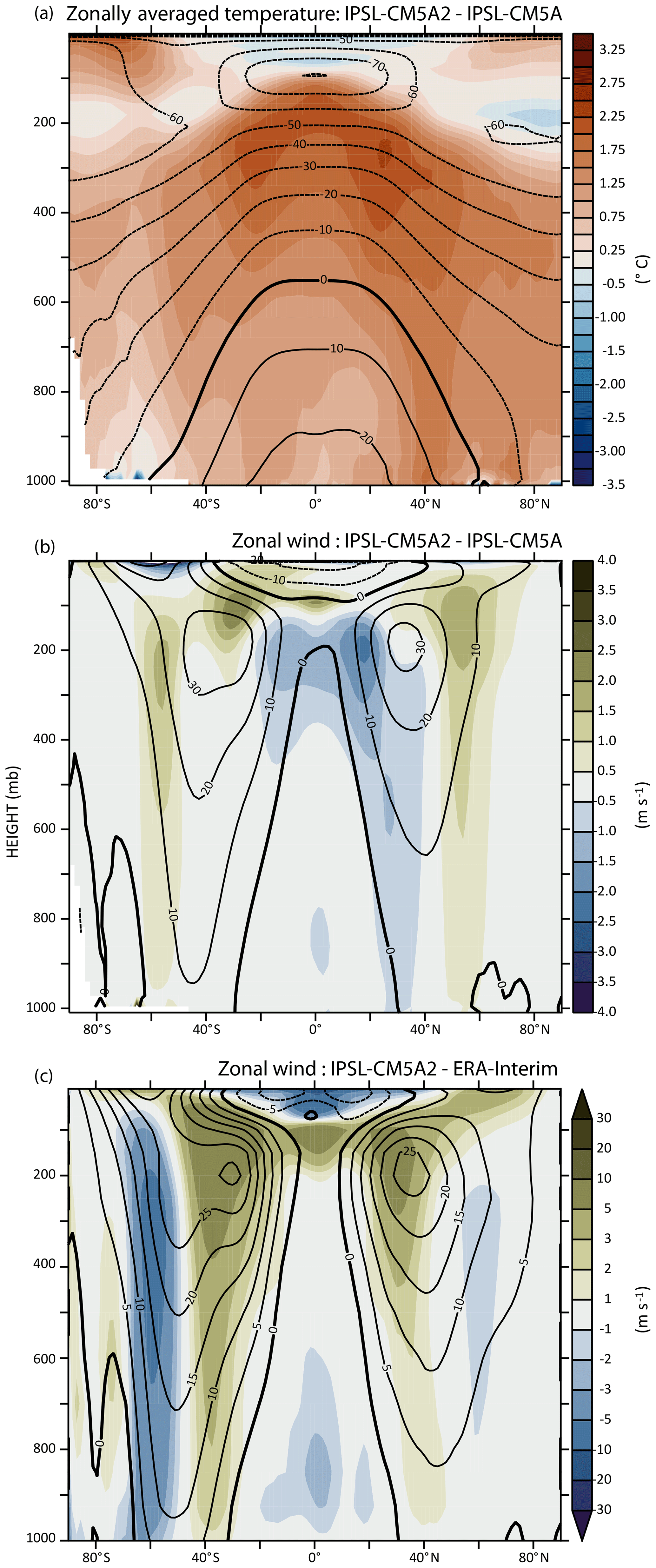
Figure 4 Zonally averaged annual anomalies between (a) IPSL-CM5A2 and IPSL-CM5A temperature, (b) IPSL-CM5A2 and IPSL-CM5A zonal wind, (c) PSL-CM5A2 and ERA-Interim (Dee et al., 2011) zonal wind. In each plot, contour lines indicate absolute values for IPSL-CM5A2, IPSL-CM5A2 and ERA-Interim, respectively.

Sea-level pressure (slp) and surface wind patterns simulated by IPSL-CM5A2 are compared to ERA-Interim reanalysis in Fig. 6. The major circulation structures, such as the subtropical highs of the Pacific and Atlantic, the December–January–February (DJF) Atlantic midlatitude low, the June–July–August (JJA) easterlies' reversal in the monsoon regions, are well captured by the model. DJF westerlies are overestimated over the Atlantic. Conversely, the model reproduces well the slp patterns at low latitudes in JJA. Simulated slp values for JJA are also underestimated between 40 and 60^∘ S and overestimated along the Antarctic coastline, in line with the zonal wind bias depicted earlier. As a consequence, westerlies' velocity maxima are restricted to 45^∘ S instead of 50^∘ S in the reanalysis (Fig. 5c, f). The southern eastern Pacific is an exception to this general pattern, as sea-level pressures are overestimated between 45^∘ S and the Antarctic coastline over this region, associated with very low surface winds velocity values. Over western Africa, the monsoonal surface wind intensity and position are well simulated, in line with the good positioning of the Saharan thermal low (Fig. 5d, e). Both winter and summer Asian monsoon surface wind patterns are correctly positioned as well, but their intensity is underestimated. Overall, the model overestimates the strength of surface easterlies, both in winter and summer. This is particularly visible over the Saharan region in DJF (Fig. 5a, b) and the northern part of South America in JJA (Fig. 5d, e).

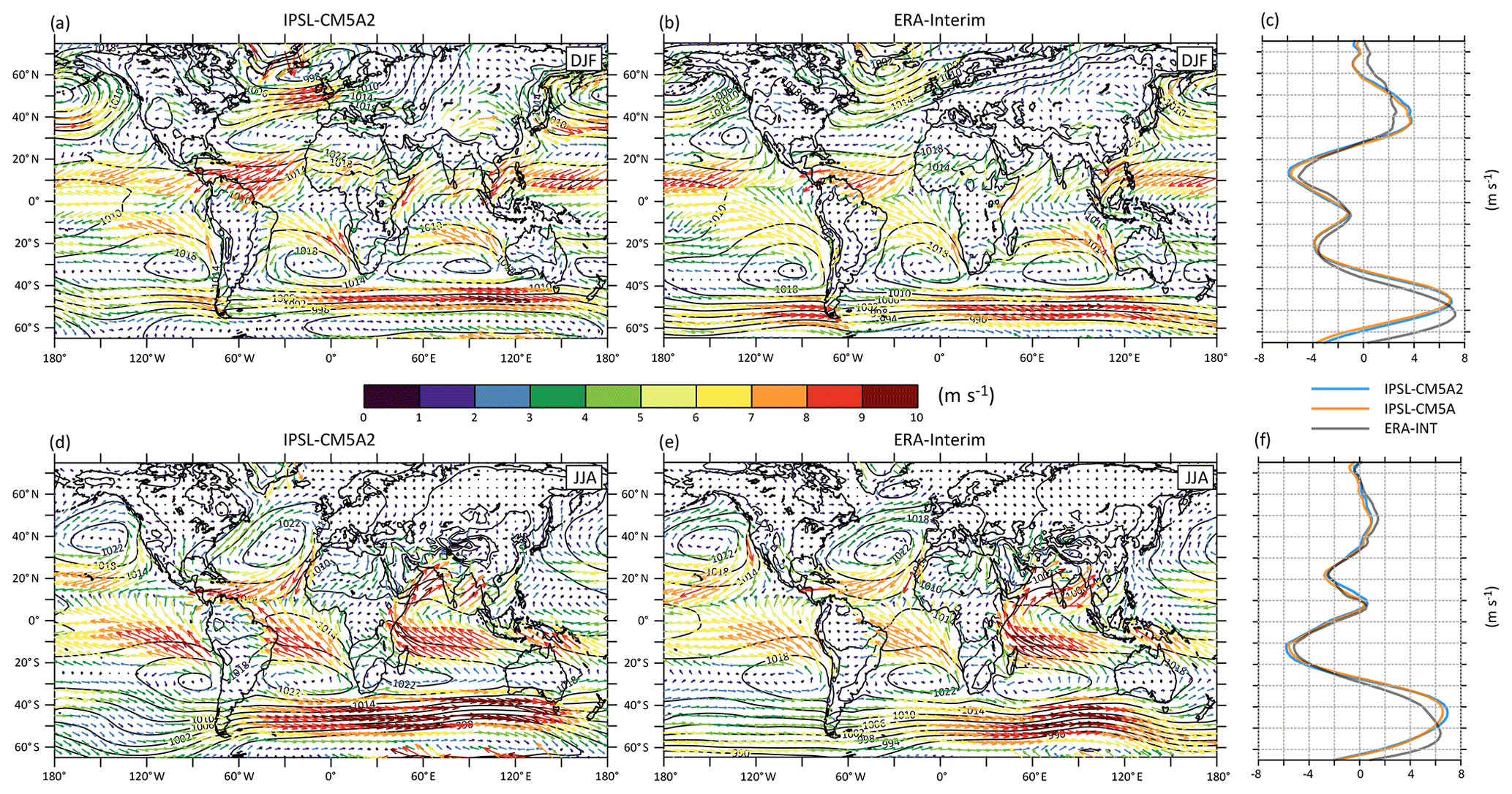
Figure 5 Mean sea-level pressure and near-surface wind velocity (colors) and direction for IPSL-CM5A2 (a, d) and ERA-Interim (b, e). (c, f) Zonally averaged near-surface wind velocity (m s⁻¹) for IPSL-CM5A, IPSL-CM5A2 and ERA-Interim. Positive (negative) values indicate eastward (westward) movement.

4.1.3 Tropical precipitation

Regarding precipitation, IPSL-CM5A2 and IPSL-CM5A essentially share the same qualities and biases, i.e., an underestimation of rainfall in the midlatitudes (20–40^∘) of both hemispheres, an overestimation of rainfall in the southern tropics, characterized on the yearly zonal average by a peak at ∼10^∘ S corresponding to a “double ITCZ” (Fig. 6e). Dry biases (−0.5 to −2 mm d⁻¹) are marked over the western edges of the northern and southern Atlantic at midlatitudes, as well as the northwestern Pacific in JJA. The regional anomaly between IPSL-CM5A2 and Global Precipitation Climatology Project (GPCP) data also shows that the tropical biases vary with longitude: namely rainfall is overestimated over the equatorial western Indian Ocean, equatorial Africa and south equatorial Atlantic (+1 to +3 mm d⁻¹) in DJF (Fig. 6a, c), whereas there is a strong underestimation of tropical rainfall over South America, specifically over the Amazon basin (down to −5 mm d⁻¹).

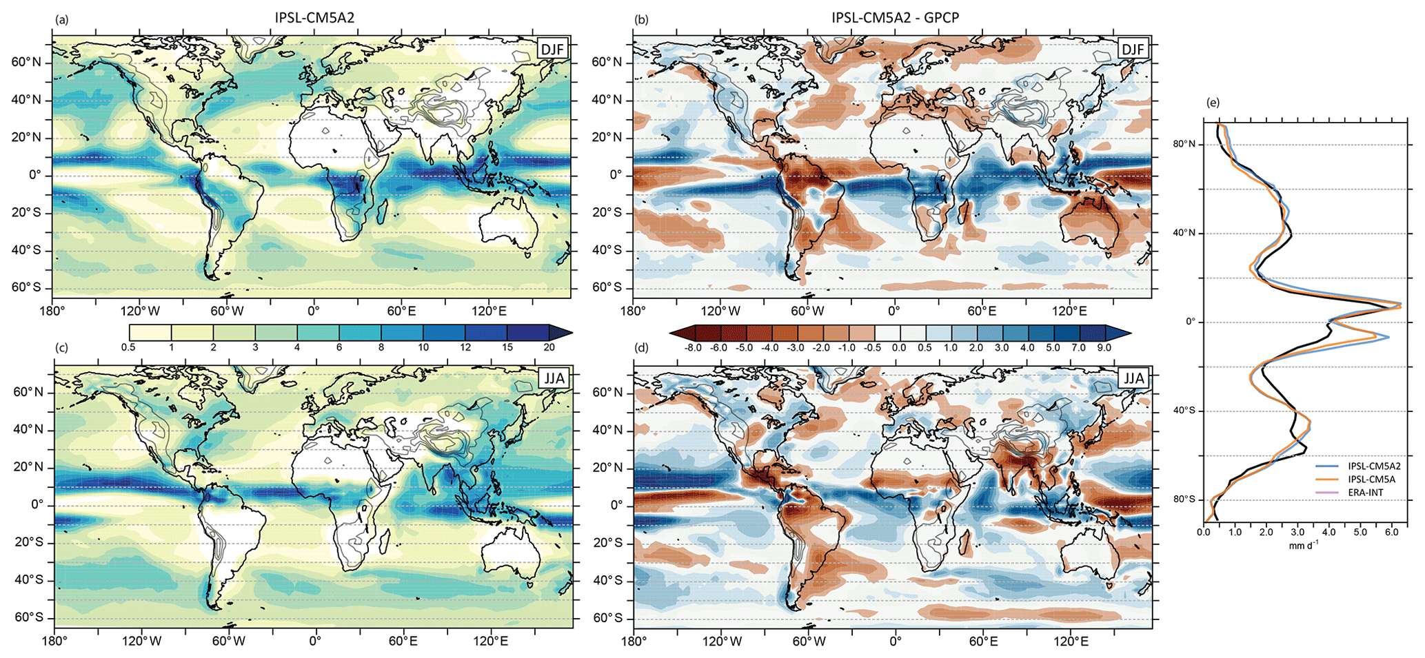
Figure 6 Seasonally averaged precipitation (mm d⁻¹) for IPSL-CM5A2 (a, c) and the anomaly between IPSL-CM5A2 and GPCP data (b, d). Top is DJF; bottom is JJA. (e) Zonal average of absolute annually averaged precipitation (mm d⁻¹) for IPSL-CM5A2, IPSL-CM5A and GPCP data.

South America (Fig. 7)

The dry bias over South America and every region of the Amazon basin is a long-standing feature of the IPSL coupled models that likely has multiple origins, as precipitation over this region depends both on moisture advection from the Atlantic (and thus from the capability of the model to reproduce correct atmospheric dynamics and SSTs) and continent recycling of water through evapotranspiration. Dufresne et al. (2013) showed that soil depth had to be increased from 2 to 4 m in IPSL-CM5A to favor seasonal water retention in the soil, allow vegetation to grow, and thereby reduce a too-strong dry bias over the Amazon. We kept this tuning in IPSL-CM5A2. Still, the seasonal 850 hPa wind divergence shows that a strong dipole between restricted convective zones and expanded subsiding zones is simulated over tropical South America (Fig. B2). This pattern induces restricted areas with strong (>8 mm d⁻¹) convective precipitation (northwestern Amazon in JJA, south-central Amazon in DJF) connected to larger zones where rainfall is limited by subsidence. The increase in the dry bias over South America between IPSL-CM5A and IPSL-CM5A2 results from a feedback loop linked to vegetation change. The tuning of the clouds produces excessive warming (Fig. 4), especially over the northwestern Amazon basin, that combines with DJF subsidence to strongly reduce rainfall amounts and thereby tropical rainforest cover (not shown).

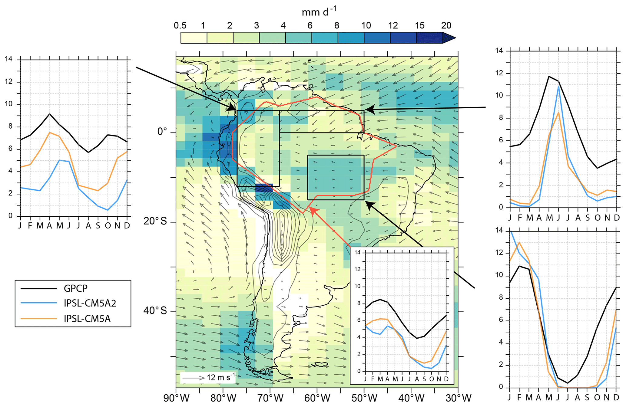
Figure 7 Rainfall patterns over South America. The map shows the precipitation annual mean (mm d⁻¹) simulated in the IPSL-CM5A2 historical experiment. The insert on the map shows the seasonal cycle over the entire Amazon basin (blue line) for IPSL-CM5A, IPSL-CM5A2 and GPCP data. Inserts at the edges of the map show the seasonal cycles for three subregions of the Amazon basins.

In line with earlier deforestation experiments carried out with the IPSL model (Davin and de Noblet-Ducoudré, 2010), such a decrease in tree cover has a strong feedback on temperature, as it leads to a decrease of latent heat flux and increase in sensible heat fluxes (overpassing the albedo increase that tends to cool surface air temperature). As an illustration, the 2 m temperature difference between IPSL-CM5A2 and IPSL-CM5A reaches +3.5 ^∘C over northwestern Amazonia, with IPSL-CM5A2 annual mean 2 m temperature reaching 29.9 ^∘C (not shown). Vegetation decrease also further reduces water recycling through lower evapotranspiration as confirmed by a supplemental historical experiment with IPSL-CM5A2 initialized with observed values of vegetation rather than the results from PREIND that shows that prescribing rainforest over the Amazon basin cools 2 m temperature by 1 to 3 ^∘C and increase annual rainfall amount by 2 mm d⁻¹ (not shown). The seasonal cycles of precipitation computed over the northern and southern parts of the Amazon basin show the simulated rainfall collapse during the respective hemispheric winters, while the year-round underestimation of rainfall in the western part of the basin seems to be related to a mislocation of rainfall that occurs on top of the Andes instead of the foothills.

Africa (Fig. 8)

Conversely, precipitation rates are overestimated over equatorial Africa. The divergence of 850 hPa wind shows that the model overestimates convergence of moist air masses south of the Equator in DJF (Fig. A3). Moreover, the +0.5 to +2 ^∘C anomalies in the eastern tropical Atlantic SST likely favor enhanced evaporation and moisture advection over the continent. Over central Africa, rainfall seasonal cycle is bimodal with two humid seasons, but the maxima lag by 1 month when compared to data. More importantly, rainfall amounts are largely overestimated by $\sim +\mathrm{66}$ % during the humid seasons. Over the western African monsoon region, IPSL-CM5A and IPSL-CM5A2 both lag the start of the rainy season, leading to an overall underestimation of rainfall before the monsoon peak. However, this rainfall maximum occurs in August as for observations, and the subsequent decrease is simulated correctly.

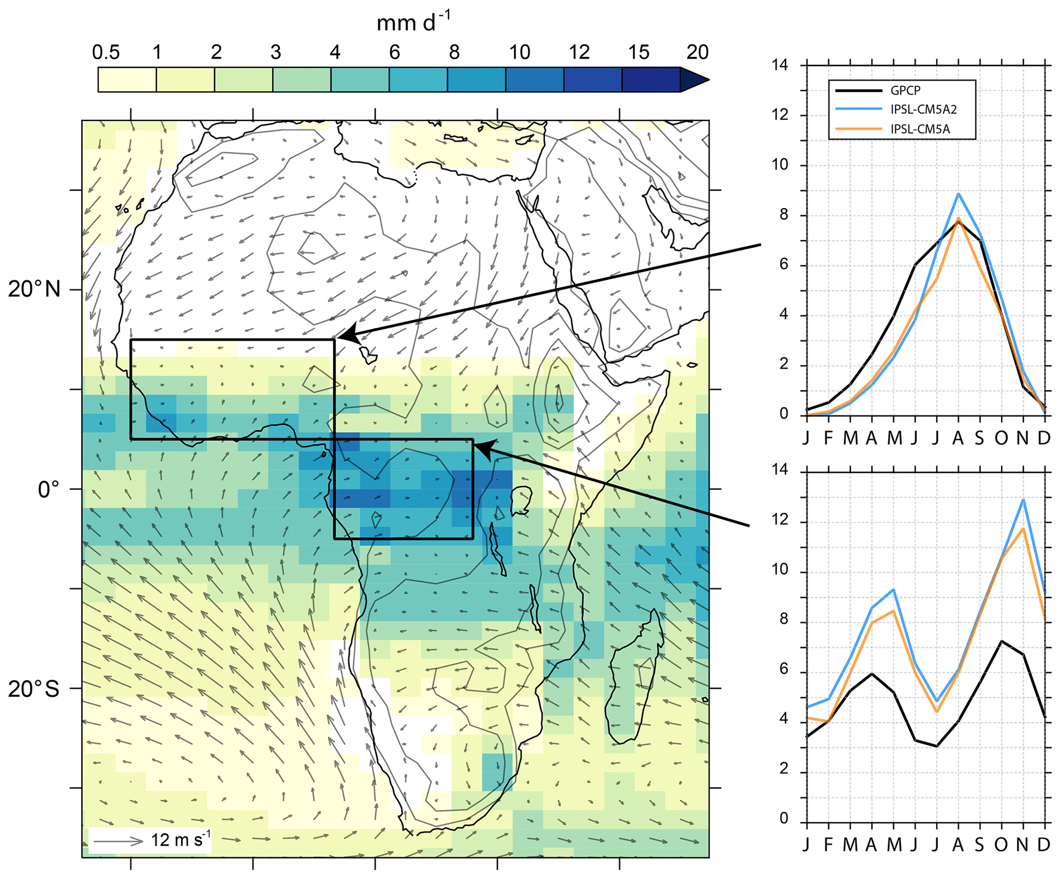
Figure 8 Rainfall patterns over Africa. The map shows the precipitation annual mean (mm d⁻¹) simulated in the IPSL-CM5A2 historical experiment. Inserts on the sides of the map show the seasonal cycle over the Congo basin and the west African monsoon region for IPSL-CM5A, IPSL-CM5A2 and GPCP data.

Indian monsoon and Indonesia (Fig. 9)

Compared to IPSL-CM5A, the Indian monsoon has been improved in IPSL-CM5A2 (Fig. 9a, b). The 1-month lag that characterized IPSL-CM5A is still present, but the amplitude of the seasonal cycle of precipitation, although still underestimated, has been enhanced, peaking at 7.3 mm d⁻¹ in August (5.6 mm d⁻¹ in August in IPSL-CM5A), closer to observations (9.3 mm d⁻¹ in July in GPCP data). This improvement is linked both to higher large-scale and convective precipitation during summer, consecutive of the enhanced hydrological cycle linked to the tuning-induced warming. However, the artificially high precipitation rates on the Himalayan foothills have not been corrected. They are made mostly of large-scale precipitation that is overestimated due to a too-strong cooling over the highest-altitude grid points.

Figure 9c shows Hovmöller diagrams for GPCP dataset compared to IPSL-CM5A2. Although at the first order, the seasonal cycle of precipitation is correctly represented over the “Maritime Continent”, IPSL-CM5A2 depicts a strong humid bias over the region (up to +5 mm d⁻¹ during the humid season). This bias has been described earlier with LMDZ pre-industrial simulations run either in atmospheric-only or fully coupled mode (Toh et al., 2018; Sarr et al., 2019) and it was shown that LMDZ systematically overestimates rainfall over both land and sea surfaces of the Maritime Continent, together with western Indian Ocean and Bay of Bengal. Given the complexity of the Indonesian region, with a myriad of islands that the model spatial resolution cannot capture, it is no surprise that rainfall is misrepresented in this model (Qian, 2008).

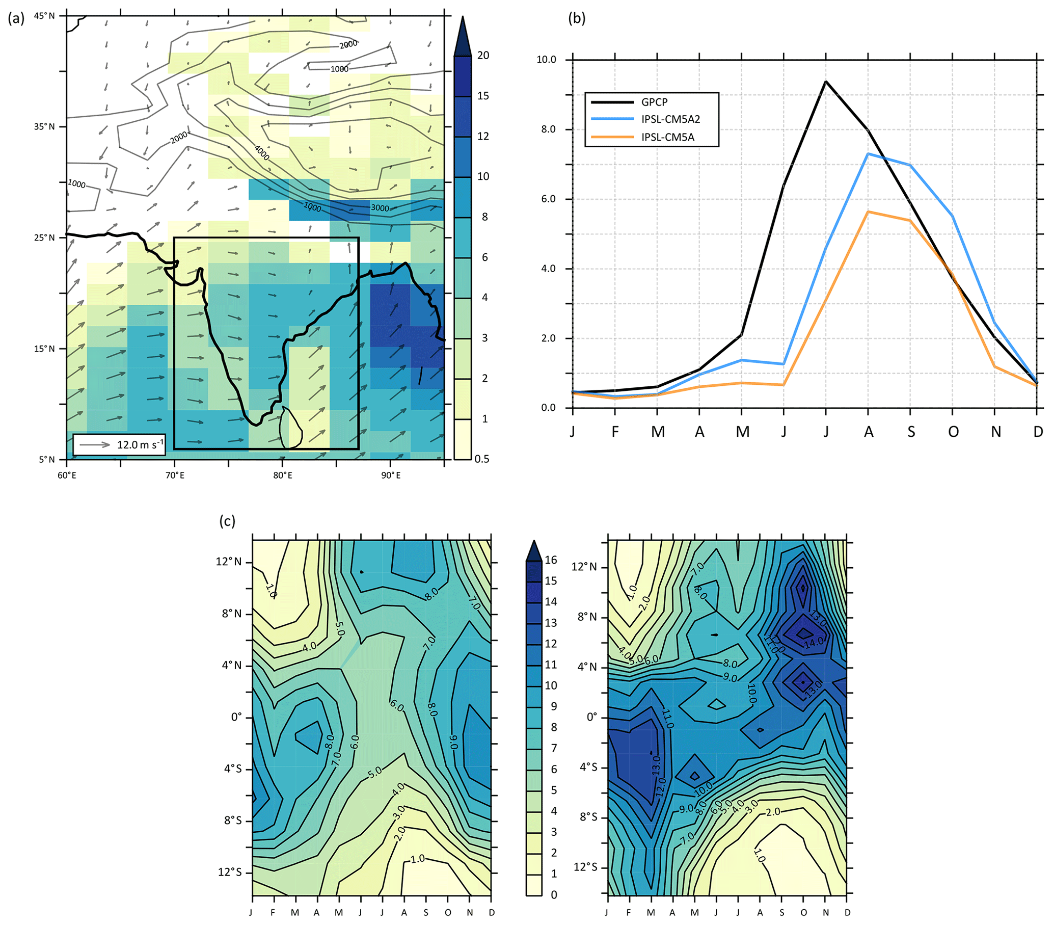
Figure 9 (a) Yearly averaged rainfall (mm d⁻¹) over the Indian subcontinent. (b) Rainfall seasonal cycle over India (black square in panel a). (c) Hovmöller diagrams of precipitation (mm d⁻¹) averaged over a 95–115^∘ E range. Left: GPCP; right: IPSL-CM5A2.

4.2 Ocean mean state and identified biases

The annual SST averaged between 50^∘ S and 50^∘ N simulated by IPSL-CM5A2 for the last decades of the historical run is 22.3 ^∘C (1 ^∘C warmer than IPSL-CM5A), a value in the higher range of CMIP5 ESMs and consistent with observations (Fig. A2).

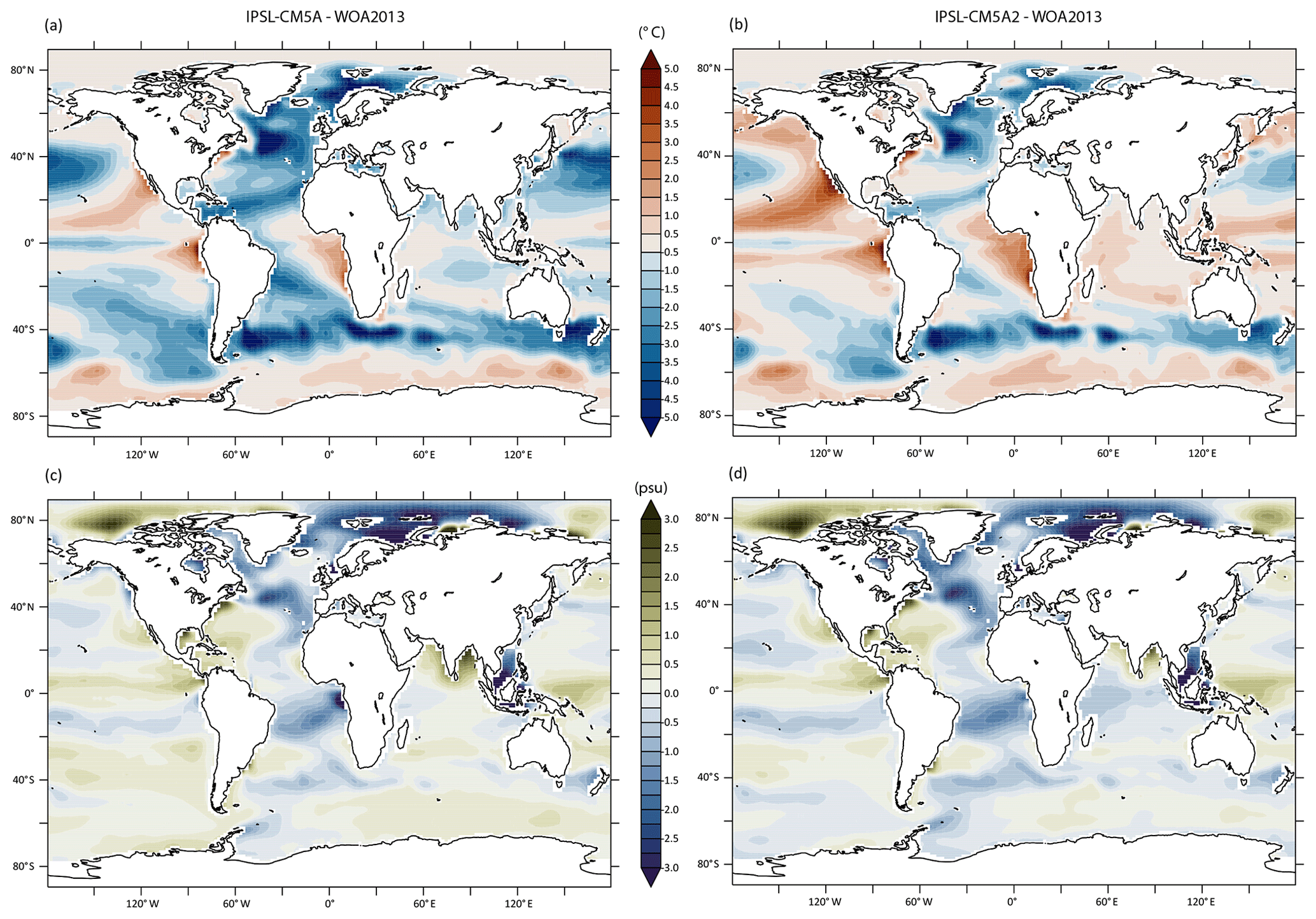
Figure 10 Yearly averaged anomalies between simulated surface temperature (a, b) and surface salinity (c, d) and WOA2013 observations (Locarnini et al., 2013; Zweng et al., 2013) for the 1980–1999 period. (a, c) IPSL-CM5A – WOA2013. (b, d) IPSL-CM5A2 – WOA2013.

The warm bias over eastern subtropical Pacific and Atlantic oceans is more marked in IPSL-CM5A2 than in IPSL-CM5A as a response to CRF tuning (Fig. 10a, b). This bias has already been reported in several coupled models using NEMO, namely CNRM-ESM1 (Séférian et al., 2016), CNRM-CM5.1 (Voldoire et al., 2013), IPSL-CM4 (Marti et al., 2010) and IPSL-CM5A (Dufresne et al., 2013). As stated in Voldoire et al. (2013), ocean-only experiments (Griffies et al., 2009) have suggested that such a warm bias was likely linked to “poorly resolved coastal upwellings and underestimated associated westward mass transport due to the coarse model grid resolution”. The 0.5–2 ^∘C warm bias over the Antarctic circumpolar current (ACC) is comparable to IPSL-CM5A and can be related to the poor simulation of the CRF over this region (Hyder et al., 2018) and the associated mispositioning of midlatitude westerlies depicted above. Conversely, the tuning has reduced the cold bias in the Pacific and Atlantic gyres. Surface salinity biases are rather similar between both models. The surface salinity anomaly follows the evaporation minus precipitation (E–P) pattern over the tropical oceans (not shown), showing the influence of the double ITCZ issue on the tropical ocean freshwater balance. Both models depict too-fresh surface waters in the northern Atlantic and locations of deep water formation (Fig. 10c, d). The ocean also depicts temperature biases at depth both in the Atlantic and Pacific oceans (Fig. 11). Zonally averaged potential temperature anomalies show that the warm bias in the northern Atlantic between 1000 and 3500 m has been amplified, as well as the warm bias in the northern Pacific, that concerns the entire water column in IPSL-CM5A2. The strong ($>+\mathrm{2.5}$ ^∘C) overestimation of temperatures in the subsurface waters of the Southern Hemisphere is almost identical in both versions of the model. The cold ($\sim -\mathrm{1}$ ^∘C) bias in the high latitudes of the Southern Hemisphere has been slightly reduced but is still present due to the lack of strong enough overturning in this region.

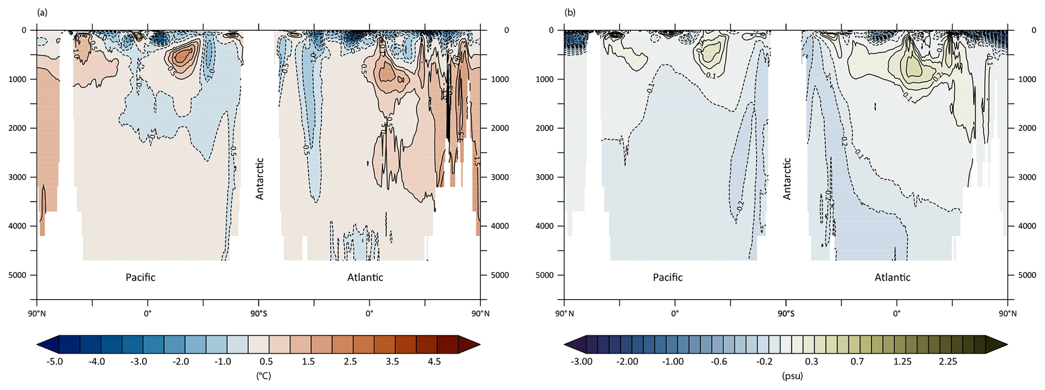
Figure 11 Longitude–depth cross section of yearly averaged anomalies between IPSL-CM5A2 temperature (a) and salinity (b) and WOA2013 observations (Locarnini et al., 2013; Zweng et al., 2013) averaged over the 1980–1999 period.

Sea-ice extent (Fig. 12) has been improved in the North Atlantic sector but remains overestimated. The Nordic Seas are covered by sea ice in winter in IPSL-CM5A, while IPSL-CM5A2 shows overestimated sea ice mostly in the Barents Sea. In the Labrador Sea, both IPSL-CM5A and IPSL-CM5A2 have overestimated sea ice, likely preventing water mass sinking and convection in this region. In contrast, sea ice is underestimated in both versions for the North Pacific sector, i.e., in the Bering and Okhotsk seas.

Figure 12 (a, b) March sea-ice cover (%) for the IPSL-CM5A (a, c) and IPSL-CM5A2 (b, d) historical runs. The black contour indicates the 15 % sea-ice cover interval in observations. (c, d) January–February–March average of mixed-layer depth (meters) for IPSL-CM5A (a, c) and IPSL-CM5A2 (b, d).

4.2.1 Ocean heat transport and meridional overturning circulation

IPSL-CM5A2 ocean meridional heat transport is higher (in absolute value) than the one simulated with IPSL-CM5A in both hemispheres (Fig. 13). This increase in the Northern Hemisphere is mainly related to the increase in the Atlantic meridional heat transport in the midlatitudes (not shown). When compared to observations, the two model versions have asymmetric biases, with the northward transport being underestimated in the Northern Hemisphere and the southward transport overestimated in the Southern Hemisphere low latitudes (between the Equator and 35^∘ S). Southward heat transport is too strong between the Equator and 40^∘ S and is in better agreement with the data than IPSL-CM5A between 40 and 60^∘ S.

Figure 13 Global meridional heat transport in the ocean, in petawatts (PW).

The AMOC is more vigorous in IPSL-CM5A2, with a maximum in depth (below 500 m) and latitude (from 30^∘ S to 60^∘ N) in pre-industrial conditions moving from 10.3±1.2 Sv (Escudier et al., 2013) to 12.02±1.1 Sv (taken for the last 1000 years of simulation; Fig. 14a). The last 20 years of the 20th century in the historical run depict a less vigorous circulation in the Atlantic, with a mean value for the AMOC index of 10.5±0.9 Sv.

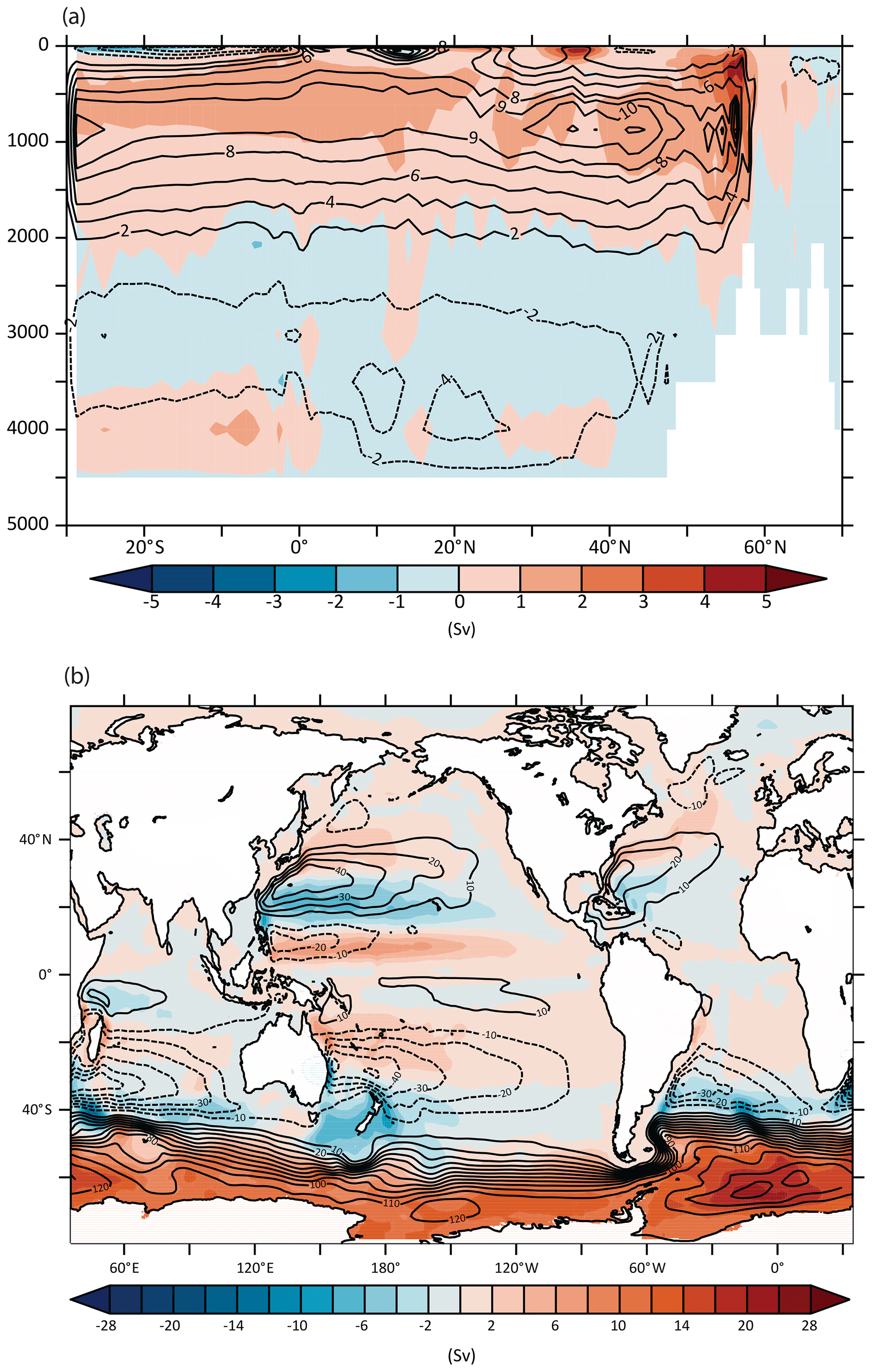
Figure 14 Atlantic meridional streamfunction (a) and global barotropic streamfunction (b) for the pre-industrial experiments at steady state (100-year averages). Color shading shows the IPSL-CM5A2 minus IPSL-CM5A anomaly. Contour lines shows the IPSL-CM5A2 values (in Sv).

The convection sites have been slightly modified between the two versions of the model. While the strongest convection was located in the North Atlantic subpolar gyre (SPG), south of Iceland, in the IPSL-CM5A version (Escudier et al., 2013), in IPSL-CM5A2, the Greenland Sea shows the deepest mixed-layer depth, which is larger than 1500 m in winter (Fig. 12c, d). Nevertheless, there is still a very active deep convection site south of Iceland, which is not realistic. The strengthening of the Nordic Seas convection can be related with the decrease of its sea-ice cover in winter (Fig. 12). As a consequence, denser water is now produced in this site, which improves the overflow through Greenland–Iceland–Scotland straits. Indeed, the water denser than 27.8 kg m⁻³ flowing southward reaches 1.5 Sv in IPSL-CM5A2, while it was only 0.2 Sv in IPSL-CM5A. It remains largely underestimated as the observations from Olsen et al. (2008) indicate around 6 Sv of overflow in total from observation-based estimates over the last few decades. Besides, the poleward shift of the westerlies in the North Atlantic stimulate a northward shift of the boundary between the Atlantic subtropical and subpolar gyres, as shown by the barotropic streamfunction anomaly (Fig. 14b). This may contribute to bringing more salt into the subpolar gyre, which may also act to intensify the AMOC in IPSL-CM5A2.

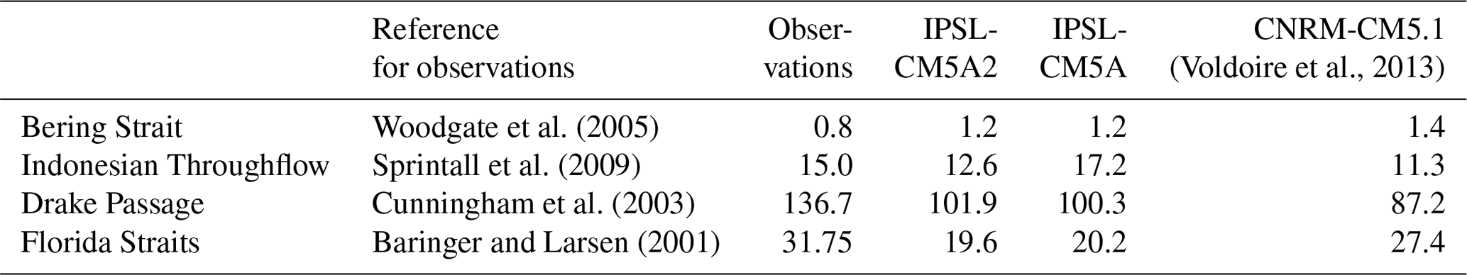
(Voldoire et al., 2013)Woodgate et al. (2005)Sprintall et al. (2009)Cunningham et al. (2003)Baringer and Larsen (2001)

Table 3 Mass fluxes through major ocean gateways in Sverdrups (Sv).

4.2.2 Fluxes in the major ocean gateways

We computed oceanic mass transport through selected longitudinal and latitudinal cross sections corresponding to the major gateways (Table 3) and compared them to IPSL-CM5A, estimates from observations and values simulated by CNRM-CM5.1, which use NEMO as well (Voldoire et al., 2013). These diagnostics highlight that the ACC is underestimated by IPSL-CM5A2 by around 25 %, as for the other configuration considered here, whereas despite the absence of high resolution and explicit resolution of Indonesian gateways, the overall Indonesian Throughflow tends to be close to observation-based estimate (underestimation of 16 %). Compared to observations and CNRM-CM5.1, the flow in the Florida Straits is quite weak (weaker than observation by 37 %), in line with the simulated “sluggish” AMOC. The increase of the AMOC from IPSL-CM5A to IPSL-CM5A2 has not been enough to strengthen this current, also largely resulting from wind forcing. The absence of resolved eddies can also play a significant role in this underestimation.

4.2.3 Net primary production (NPP)

To illustrate some of the capabilities of IPSL-CM5A2, we also evaluate the simulated oceanic NPP (Fig. 15). The global integrated NPP over the historical period (here averaged over 1980–1999 from the historical simulation) is 47.5 PgC yr⁻¹, which is a strong increase when compared to 30.9 PgC yr⁻¹ simulated for IPSL-CM5A (Bopp et al., 2013), making IPSL-CM5A2 closer to the 52.1 PgC yr⁻¹ global estimate based on SeaWiFS remote-sensing observations (Behrenfeld and Falkowski, 1997). The representation of NPP at the spatial scale compares well to observation-based estimates for the tropical and Southern Hemisphere but depicts large biases in the Northern Hemisphere, especially in the North Atlantic where NPP is largely underestimated (Fig. 15c).

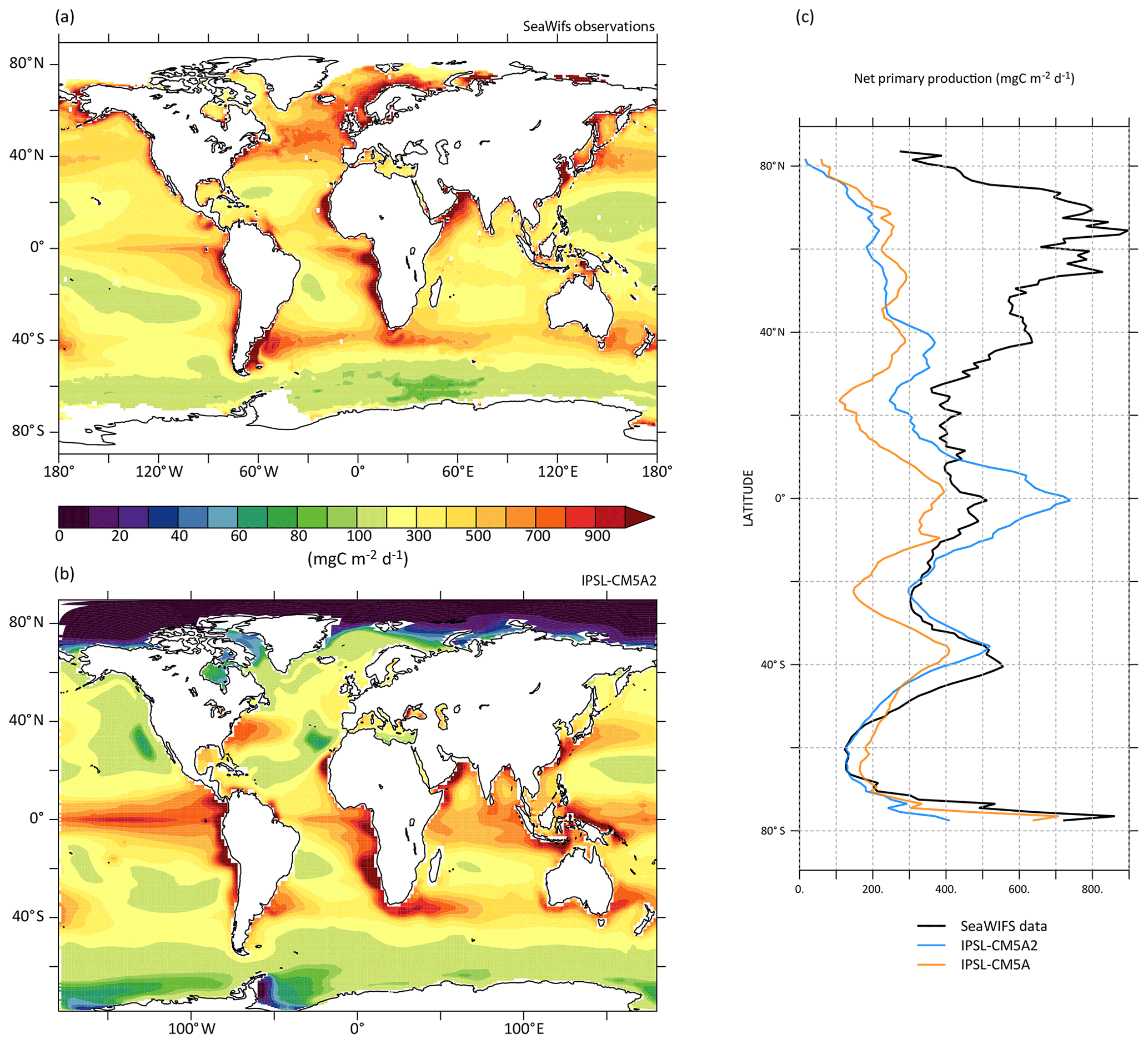
Figure 15 Mean vertically integrated NPP retrieved from SeaWiFS observations (a) and simulated by IPSL-CM5A2 (b). (c) Latitudinal variations of mean vertically integrated NPP, zonally averaged, for SeaWiFS (black), IPSL-CM5A (orange) and IPSL-CM5A2 (blue).

4.2.4 Ocean variability

The main modes of variability of the AMOC are analyzed with an empirical orthogonal function (EOF) of the yearly Atlantic meridional overturning streamfunction (Fig. 16, top). The first EOF is a monopole in IPSL-CM5A and IPSL-CM5A2, but IPSL-CM5A2 shows less loading in the subpolar gyre between 40 and 60^∘ N. The associated principal component shows a significant 20-year variability in the case of IPSL-CM5A. Such variability was previously linked to advection of surface salinity anomalies from the western boundary to the eastern Atlantic (Escudier et al., 2013) and westward-propagating planetary waves in subsurface (Ortega et al., 2015). North Atlantic observations (Vianna and Menezes, 2013; Swingedouw et al., 2013) and proxy records indicate a 20-year preferential variability in this region in the atmosphere (Chylek et al., 2011), sea ice (Divine and Dick, 2006) and the ocean (Sicre et al., 2008; Cronin et al., 2014). However, the peak of variability at 20-year timescale is not significant any more in IPSL-CM5A2 (see spectra in Fig. 16c–d). This difference can be explained by the different tuning of the two model versions.

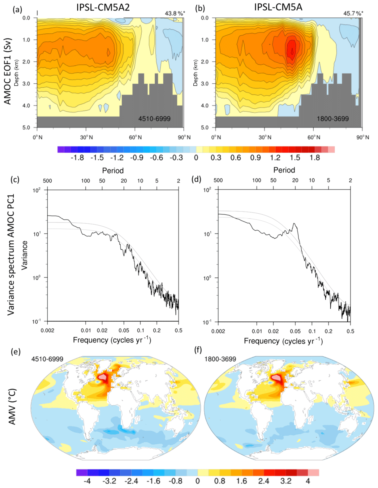
Figure 16 (a, b) Spatial patterns of the leading EOF of the yearly AMOC computed from 2490 years of the IPSL-CM5A2 PREIND (model years 4510 to 6999) and from 1900 model years of the IPSL-CM5A PREIND (model years 1800 to 3699), respectively. The patterns are given in Sv for 1 standard deviation of the corresponding principal component, and the amount of variance explained by the pattern is given in the top right of each panel. Panels (c) and (d) show the variance spectra of the associated leading principal components, respectively. The dashed lines show the 95 % and 99 % confidence levels of the best-fit first-order Markov red noise spectrum, respectively. (e, f) Atlantic multidecadal variability (AMV) pattern, in K, in IPSL-CM5A2 PREIND and IPSL-CM5A PREIND, respectively, from the same model years as above. The AMV was calculated from the low-pass-filtered (61-month running mean) North Atlantic SST in 0–60^∘ N, 80^∘ W–0^∘ E. The AMV pattern is given by the regression of the SST onto the AMV index.

Gastineau et al. (2018) used IPSL-CM5A-MR, a variant of IPSL-CM5A with an improved horizontal resolution in the atmosphere ($\mathrm{2.5}{}^{\circ }\times \mathrm{1.25}{}^{\circ }$ vs. $\mathrm{3.75}{}^{\circ }\times \mathrm{1.87}{}^{\circ }$) and also found that a warmer mean state led to a reduction of the 20-year variability in IPSL-CM5A-MR. Such a warmer mean state modifies the subpolar gyre currents and the subsurface stratification in the eastern Atlantic Ocean where the mixed layer is deepest in IPSL-CM5A models. These changes were suggested to explain a smaller growth of baroclinic instabilities triggering the propagation of westward-propagating anomalies (Gastineau et al., 2018). It is therefore likely that the different tuning of IPSL-CM5A2 led to similar changes. The SST associated with the first principal component of the AMOC also shows weaker SST anomalies in the subpolar gyre when compared to IPSL-CM5A (not shown). The AMV patterns are similar in IPSL-CM5A and IPSL-CM5A2, with a slightly more intense subpolar gyre SST (6.8 ^∘C vs. 6.2 ^∘C for the maximum value in the subpolar gyre) in IPSL-CM5A2. Larger positive SST anomalies in IPSL-CM5A2 are also simulated in the Nordic Seas and Irminger Sea associated with the AMV. The larger AMV in IPSL-CM5A2 is consistent with the smaller sea-ice cover in the North Atlantic and a more intense signature of the atmospheric forcing. Yet, the observed AMV pattern computed from the historical period (1870–2008) using a similar methodology does not show such an intense subpolar pole: the SST anomalies in the subpolar region are only twice as intense is the tropical ones (Deser et al., 2009).

The Pacific variability in IPSL-CM5A2 is identical to that found in IPSL-CM5A. The El Niño–Southern Oscillation (ENSO) is characterized by the NINO3.4 time series. IPSL-CM5A and IPSL-CM5A2 show a similar power spectrum (Fig. B3a, c, e) which is comparable to observations (Bellenger et al., 2014). Both versions have the same bias in the seasonal phase locking (Fig. B3b, d, f), as the monthly standard deviations are larger in May and June in CM5A and CM5A2, while the observed maximum is in January and December. The ENSO impacts are evaluated using spatial composites of the SST over ocean, 2 m air temperature over land and sea-level pressure. The composites are built using the NINO3.4 time series and calculating the difference of all years where the NINO3.4 exceeds 1 standard deviation, minus years less than 1 standard deviation. Figure B4 illustrates that the ENSO impacts are identical in both versions of the model, with a systematic bias in the position of the Pacific equatorial SLP anomalies which extend too far west toward the Pacific warm pool. However, the SLP anomalies display a realistic pattern in the Northern Hemisphere and Southern Hemisphere, with the associated Pacific North American and Pacific South American patterns, as in other CMIP5 models (Weare, 2013). The Pacific Decadal Oscillation (PDO) was also calculated as the first EOF of the monthly Pacific SST anomalies north of 20^∘ N (Fig. B5), which illustrate a pattern with positive SST anomalies over the equatorial Pacific, negative anomalies in the northwest Pacific and a horseshoe pattern of positive SST anomalies in the Northern Hemisphere. The IPSL-CM5A model generally simulates the characteristics of the observed PDO, as found by Fleming and Anchukaitis (2016) or Nidheesh et al. (2017), as well as the associated anomalies in the Atlantic and ocean basins. The IPSL-CM5A2 version simulates a PDO nearly identical to that of IPSL-CM5A, so that the mean state changes have no impact on the PDO state.

5 IPSL-CM5A2 for deep-time paleoclimate modeling, a case study

This section depicts both the technical developments and the choices to be made regarding boundary conditions for a typical deep-time simulation with IPSL-CM5A2. We describe the generation of a new grid for the ocean model for deep-time applications and the generation of boundary conditions, component-wise. To illustrate our point, we run a 3000-year long numerical simulation of the Cretaceous as a case study. We present a very brief analysis of the model time series to illustrate the long adjustment required to reach equilibrium in deep-time simulations. As the focus of the paper is the description of IPSL-CM5A2, we only provide a very basic description of the simulated climate. We refer readers to Laugié et al. (2020) for a detailed description of a Cretaceous simulation run with IPSL-CM5A2.

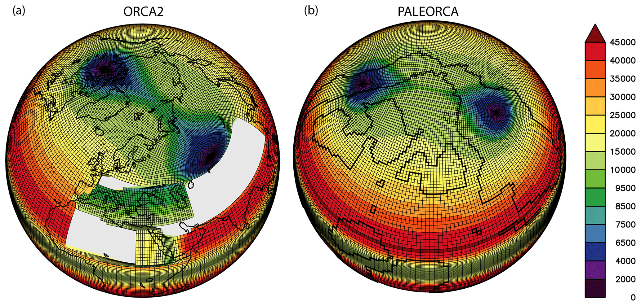
Figure 17 Comparisons of ORCA2 grid (a) and PALEORCA grid (b). Color shading shows spatial resolution (km²). Grey-shaded areas on ORCA surround the refinements of the grid over the Mediterranean, Red, Black and Caspian seas. The centers of the blue areas show the two poles that have been rotated in PALEORCA.

5.1 Generating a new grid for NEMO

In addition to the aforementioned computational performance, technical issues related to the oceanic component of the model also have long prevented the use of any version of the IPSL ESM for deep-time climate modeling. The main lock was that NEMO runs on a tripolar grid (ORCA2, with two poles in the Northern Hemisphere and one over Antarctica) that was designed, amongst other objectives, to avoid any singularity points on the computational domain (i.e., the ocean domain) (Madec, 2015; Madec and Imbard, 1996). Specifically, north of 20^∘ N, the mesh is made of a series of embedded ellipses, the foci of which are the two north poles of the grid that are by design placed over continents (Fig. 17a). Southward the grid is a Mercator (i.e., identical longitudinal and latitudinal grid spacing) grid, defined down to 78^∘ S, except from local refinements applied in the tropics, so that the meridional resolution reaches 0.5^∘ at the Equator and over the Red, Black, Caspian and Mediterranean seas where resolution is about 1^∘.

Because the grid poles are located over North America, Asia and Antarctica, changing the land–sea mask to account for continental drift can shift the singularity points into the computation domain. In addition, a number of ocean routines include hard-coded specifications that apply to some narrow modern straits, such as the Strait of Gibraltar. In these regions, the resolution of the grid is much larger than the width of the straits, thereby requiring the outflow of water to be prescribed. Although needed to better simulate modern climates, these features are irrelevant for deep-time simulations. To overcome these issues, we design a new PALEORCA grid based on techniques and code designed by G. Madec and A. Sellar. The Southern Hemisphere (SH) pole is conserved, which restricts the application of IPSL-CM5A2 to the last 100 million years (Antarctica has been located over the South Pole since approximately the mid-Cretaceous). In the Northern Hemisphere (NH), new ellipses are computed, changing the location of the two singularity points to eventually obtain a grid that can effectively be used for the last 100 million years. To this end, and because the grid structure requires both NH poles to be diametrically opposed and limits the range of latitude in which the location of the poles can be chosen, the two poles are placed, respectively, at 60^∘ N, 106^∘ E, and 60^∘ N, 74^∘ W (Fig. 17b). Abovementioned refinements over the Mediterranean and Eurasian seas are removed, but the tropical refinement is kept. We also take advantage of the well-defined coding guidelines of NEMO to create a PALEORCA configuration within the available oceanic configurations of the model. In this configuration, no hard-coded water exchanges across the globe are prescribed.

5.2 Application: generating boundary conditions for deep-time climate modeling

The Cretaceous is historically known for its warmer-than-present climatic state without permanent ice sheets at the poles. Here, we present a simulation of the Turonian stage (circa 90 Ma), during which the apex of the Cretaceous warmth was reached. CO₂ estimates reconstructed from proxy-based studies vary from 500 ppm to >2000 ppm with large uncertainties (Wang et al., 2014). In our simulation, we impose an atmospheric CO₂ concentration of 1120 ppm (4× pre-industrial values) and we remove polar ice sheets. In addition, we keep the modern orbital configuration as no numerical solution for orbital parameters exists for the Cretaceous (Laskar et al., 2004). The basis of our Turonian configuration is the Cenomanian/Turonian paleogeography of Sewall et al. (2007).

5.2.1 Oceanic boundary conditions

Bathymetry. The Turonian bathymetry (Fig. 18b) is obtained from the merging of two datasets. First, the regular longitude–latitude Cenomanian/Turonian paleogeography from Sewall et al. (2007) is masked over continental areas and remapped onto the curvilinear PALEORCA grid. Given that the bathymetry of the Pacific and Indian oceans is mostly flat (without ridges) and deep (∼5000 m), in Sewall et al. (2007), we have decided to merge the more recent bathymetric dataset of Müller et al. (2008) with the land–sea mask and continental margins of Sewall et al. (2007) to create a more realistic deep bathymetry. Handmade corrections are then applied to the bathymetry to ensure that narrow straits (e.g., west Africa) are at least two grid points wide. This avoids the implementation of specific hard-coded schemes in the model to represent water advection across those straits.

Geothermal heating. The model modern boundary conditions include a realistic map of geothermal heating, whose impact on the ocean abyssal dynamics is non-negligible (Emile-Geay and Madec, 2009). As the geothermal heat flow q(t) can be related to the ocean lithosphere age t, we construct a geothermal heating map for the Turonian based on the reconstruction of the Turonian ocean crustal age of Müller et al. (2008). We derive the geothermal heat flux using the age–heat flux relationship of the Stein and Stein (1992) model.

For t≤55 Ma,

$$\begin{array}{}\text{(2)}& q\left(t\right)=\mathrm{510}{t}^{\mathrm{1}/\mathrm{2}}.\end{array}$$

For t>55 Ma,

$$\begin{array}{}\text{(3)}& q\left(t\right)=\mathrm{48}+\mathrm{96}{e}^{-\mathrm{0.0278}t}.\end{array}$$

In regions where crust age is missing in the Müller et al. (2008) dataset, we impose the minimal geothermal heat flux obtained with the above equations. The geothermal heating map created is then remapped on the PALEORCA grid and we limit the maximal heat flux to 400 mW m⁻² because the Stein and Stein (1992) parameterization becomes singular for young ages (Emile-Geay and Madec, 2009).

Tides. Modern boundary conditions also include forcings of the dissipation associated with internal wave energy for the M2 and K1 tides component; see de Lavergne et al. (2019). Here, in the absence of an appropriate model to estimate M2 and K1 dissipation values for the Cretaceous, we neglect this forcing and set these fields to zero.

Initial conditions. Salinity is initialized as a uniform value of 34.7 per mil equal to the modern mean ocean value (Lunt et al., 2017). The ocean initial temperature follows a slightly altered formulation of the zonally symmetric temperature distribution proposed by Lunt et al. (2017): if depth≤1000 m,

$$\begin{array}{}\text{(4)}& T=\mathrm{10}+{\displaystyle \frac{(\mathrm{1000}-\mathrm{depth})}{\mathrm{1000}}}\mathrm{25}\cos \mathit{\phi };\end{array}$$

if depth>1000 m,

$$T=\mathrm{10}.$$

These initialization temperatures are quite high, as the ice-free Cretaceous periods have been shown to have much warmer oceans than at present, associated with high atmospheric pCO₂. No sea ice is prescribed at the beginning of the simulation.

5.3 Continental boundary conditions

Topography. We use the Cenomanian/Turonian topography from Sewall et al. (2007) but modify the Antarctic continent because the PALEORCA mesh is not defined beyond 78^∘ S, which corresponds to the maximal extent of the modern Antarctic coastline (including ice shelves). This requires that the Antarctic coastline reaches at least the same latitude for paleoclimate simulations, which is not the case in the Cenomanian/Turonian continental configuration of Sewall et al. (2007). We therefore impose the maximal Antarctic topography proposed by Wilson et al. (2012) for the Eocene–Oligocene, which has the advantages of meeting the required Antarctic coastline criterion and is a relatively recent estimate of a deep-time Antarctic topography, which remains generally poorly constrained. The final topography/bathymetry is shown in Fig. (18b). LMDZ requires a 10 min global elevation dataset to compute subgrid-scale parameters (elevation standard deviation, slope, peaks and valleys) that are needed to compute surface roughness length as well as to activate orographic drag parameterizations (Lott and Miller, 1997). As the paleotopography provided by Sewall et al. (2007) is $\mathrm{2.8}{}^{\circ }\times \mathrm{1.4}{}^{\circ }$ in resolution, we simply artificially upscaled it to a 10 min resolution through the use of climate data operator (cdo) remapping tools (Schulzweida, 2019).

River routing. The river routing system (i.e., length of rivers, direction of flows, locations of river outflows) is constructed by first upscaling the low-resolution topography of Sewall et al. (2007) to a $\mathrm{1}{}^{\circ }\times \mathrm{1}{}^{\circ }$ resolution and then using the Wang and Liu (2006) algorithm within the QGIS software (QGIS Geographic Information System, Open Source Geospatial Foundation project; http://qgis.osgeo.org, last access: 4 November 2019). This algorithm ensures that inland depressions are filled and therefore that all continental freshwater is routed to the ocean in the coupled model.

Figure 18 Topography (a) and bathymetry (b) (in meters) imposed for the Cretaceous simulation.

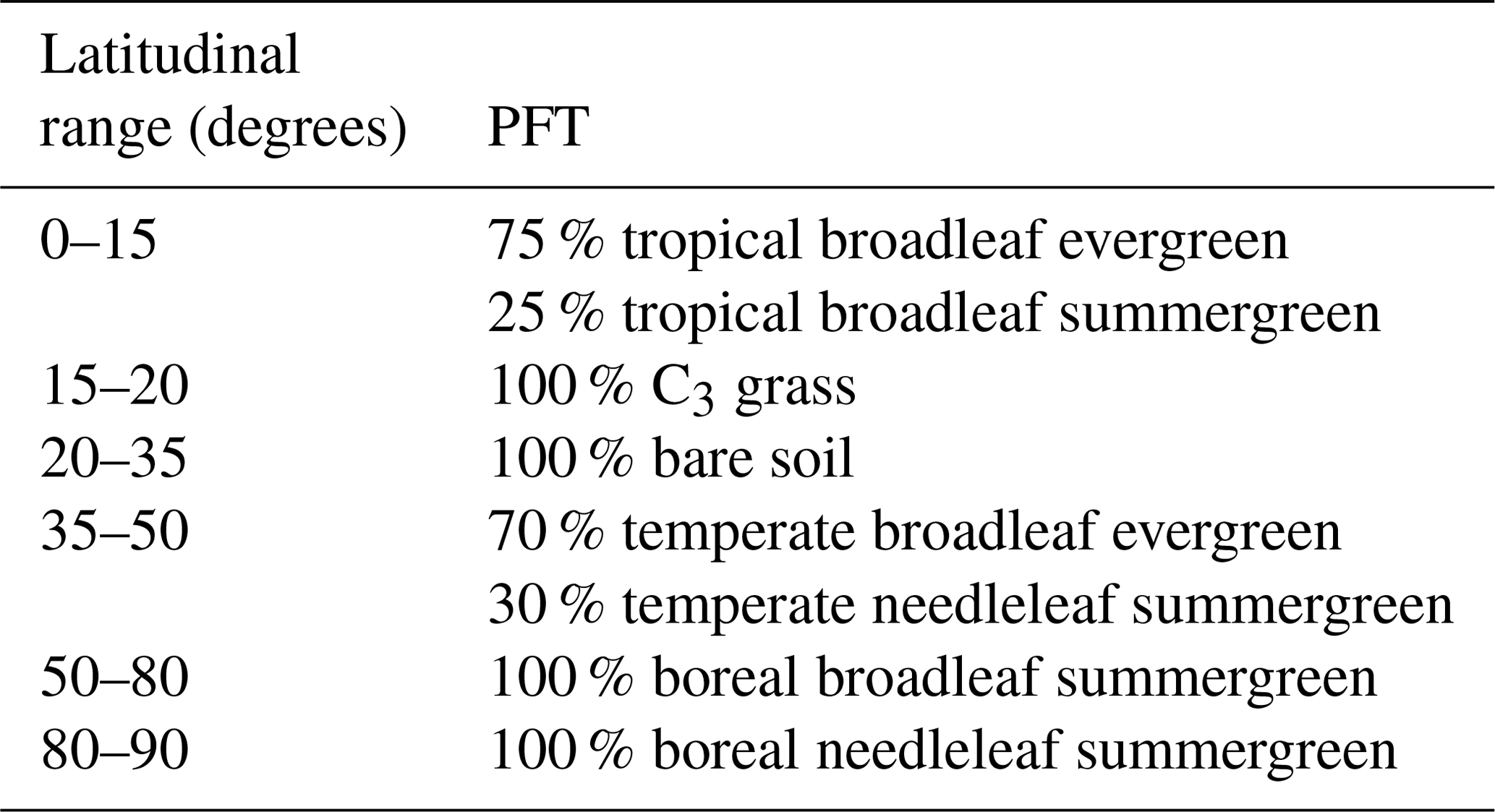
Vegetation. In the absence of globally consistent vegetation reconstructions for the Turonian, the imposed vegetation follows a very simple latitudinal distribution of plant functional types (Table 4).

Table 4 Prescribed plant functional types as a function of the latitude.

5.4 Results of the case study experiment

5.4.1 Equilibrium

Time series of SST and t2m shows the strong model departure from the initial conditions in the first centuries of the simulation (This departure is also observed in Q^TOA time series, Fig. C1). After 3000 years, SST and t2m are adjusted at 28.3 and 26 ^∘C, respectively (Fig. 19e). OHC of the first 300 m is stabilized as well. The long-term adjustment of the ocean is, as for our initial pre-industrial experiment, driven by the initial radiative unbalance resulting from the initial ocean temperatures and the greenhouse forcing. The vertical cross sections at initial and final states of the experiment shows the spatial patterns of adjustment of ocean temperature and salinity (Fig. 19a, b, c, d). The constant salinity together with the latitudinal profile of temperature imposed as initial conditions also induce a latitudinal gradient in seawater density and thereby an adjustment of ocean dynamics. Surface salinity and temperature are also adjusted driven by the precipitation minus evaporation balance (PE) and freshwater inputs from river routing (see the next section) plus radiative balance. Contrary to surface signals, the total OHC shows that the deep ocean is still adjusting after 3000 years (Fig. 19e), showing the need for very long integrations when one models deep-time paleoclimates.

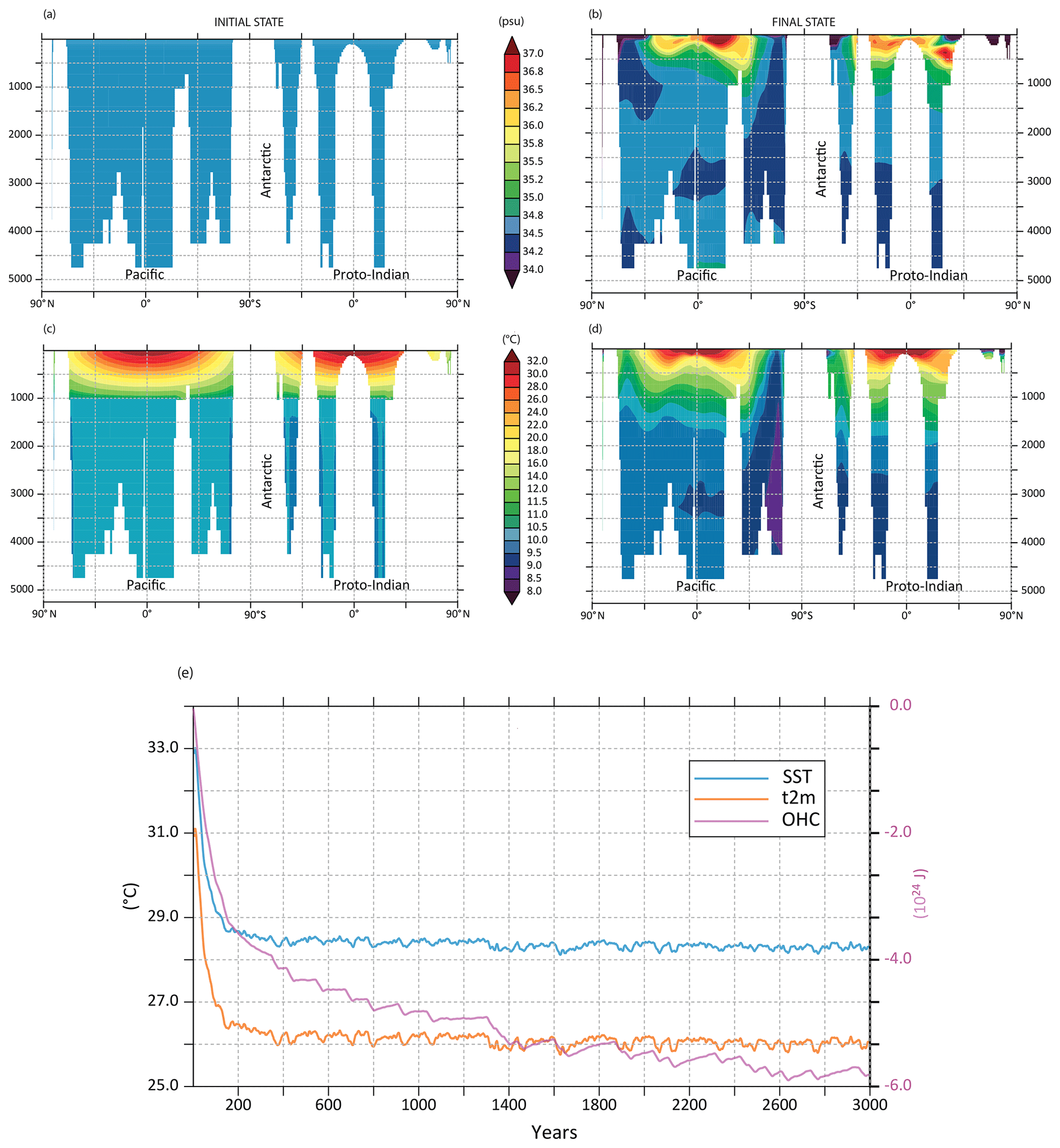
Figure 19 Adjustment of the Cretaceous simulation over 3000 years. Latitudinal cross section of initial (a, c) and final (b, d) states of salinity (top, PSU) and temperature (bottom, ^∘C) for the Cretaceous simulation. (e) Time series of SST (^∘C), t2m (^∘C) and total OHC (J).

5.4.2 Mean surface climate

The elevated values of SST and t2m at equilibrium are primarily explained by the high atmospheric CO₂ concentration prescribed. In the ocean, warmest temperatures (>36 ^∘C) are found in the equatorial band in the Atlantic and Indian oceans as well as in the western Pacific (Fig. 20a, b), whereas the eastern equatorial Pacific is cooler by a few degrees. The Southern Ocean is relatively warm (>10 ^∘C) as is the North Pacific, while the Arctic Ocean exhibits the coldest surface temperatures (reaching less than 8 ^∘C at the highest latitudes). There is no sea ice formed in the polar oceans. In continental areas, the radiative impacts of the high atmospheric CO₂ concentration and the absence of ice sheets also substantially affect the mean annual t2m. Values >40 ^∘C are found in equatorial Africa, South America and southeastern Asia, whereas below 0 ^∘C mean annual continental t2m values are only located in Antarctica (Fig. 20b). The winter season yields well-below-freezing t2m over large parts of the NH high latitudes, with lowest values in northern Siberia. Similarly, the whole Antarctic continent suffers below-freezing t2m, with values below −16 ^∘C over large parts of the continental interior (Fig. C2). In the summer, however, Antarctic t2m values are mostly above 20 ^∘C and reach up to more than 28 ^∘C close to the modern Weddell Sea (not shown). Tropical continents are affected by extremely high summer t2m reaching more then 44 ^∘C, whereas NH high latitudes exhibit the lowest summer values with <16 ^∘C in northern Siberia.

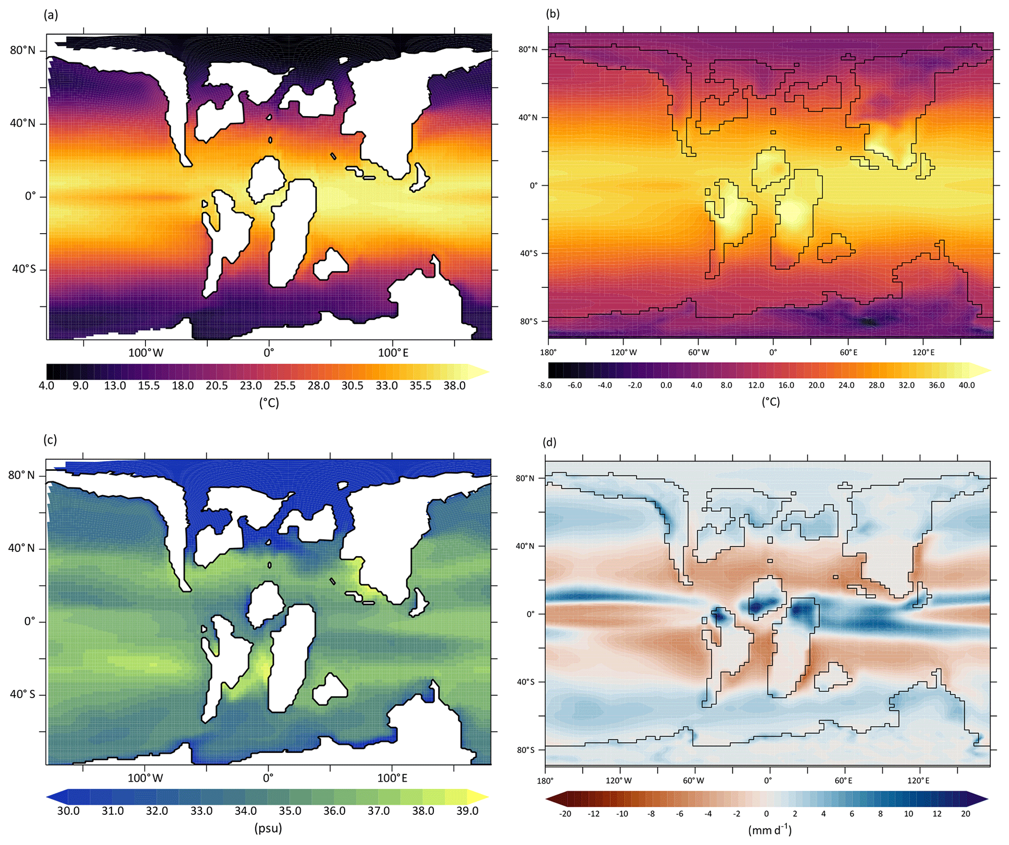
Figure 20 Climate mean state of the Cretaceous experiment after 3000 years: (a) SST (^∘C), (b) t2m (^∘C), (c) SSS (PSU) and (d) PE (mm d⁻¹).

Mean annual PE shows expected patterns across the globe (Fig. 20d), including the double ITCZ as in the pre-industrial and historical simulations. Net evaporation areas located at subtropical latitudes under the descending branch of the Hadley circulation and net precipitation areas located in the equatorial band (except in the equatorial Pacific and Atlantic) and in the midlatitudes to high latitudes. Note the particularly dry tropical continental regions of Africa and South America, which are the results of their more southern position during the Cretaceous (the same is true for south Asia in the Northern Hemisphere).

PE generally explains well the patterns of open-ocean sea-surface salinities (SSSs; Fig. 20c). Highest SSSs are thus found in the subtropical areas, whereas lower values are found in the midlatitudes to high latitudes and in the equatorial band. This spatial SSS distribution is altered by the supply of water from continental rivers. The very high amount of precipitation occurring in the equatorial band over India and northern Africa indeed increase the freshening of nearby coastal waters. Low-salinity waters are also found in the Australian–Antarctic sector of the Indian Ocean and in the Arctic Ocean, where large paleorivers can supply significant amounts of freshwater to the ocean. The relative isolation of the Arctic from the global ocean limits possible exchanges of water and therefore may amplify the freshening of this basin. The Pacific sector of the Southern Ocean is more saline than other corresponding high-latitude oceanic regions (North Pacific, Atlantic and Indian Ocean parts of the Southern Ocean) with SST of similar or lower values. The winter cooling of the dense surface waters in this region therefore leads to deep water formation as shown by the winter deepening of the mixed-layer depth (Fig. C3). Contrary to the modern state, there is no deep water formation in the Northern Hemisphere, in relation to the peculiar Turonian paleogeography, in which the northern Atlantic is only partially open and NH landmasses reach low latitudes.

This simulation, and by extent the overall response of IPSL-CM5A2 to a Cretaceous paleogeography without ice sheets and elevated CO₂ levels, would need to be evaluated in more details against previous work and proxy data. Still, the basic analysis presented here demonstrates that the mean climate simulated by our model shares many similarities with that simulated by other investigations of Cretaceous warmth with coupled models (Niezgodzki et al., 2017; Tabor et al., 2016; Upchurch et al., 2015). It therefore suggests that our goal of adapting the IPSL ESM to deep-time boundary conditions has been reached with success.

6 Conclusions

This article aimed at providing a detailed description of the building of the IPSL-CM5A2 ESM, developed with the aim of performing multi-millennial Earth system simulations. We expect IPSL-CM5A2 to be used mostly for deep-time paleoclimate modeling and, given its reasonable computing performance, attempts at transient simulations for the Quaternary and the future. Starting from IPSL-CM5A, our goal to obtain a faster model with reduced biases has been reached successfully. IPSL-CM5A2 pre-industrial integration shows a reduced cold bias, no drift in the OHC after 1500 years and reasonable energy leaks and salinity drift. Despite persistent biases in the tropics, the historical runs also show a more vigorous AMOC, together with better-located westerlies. The simulation of global NPP, although still underestimated, has been largely improved. Our case study for the Cretaceous shows the numerous hurdles, often undocumented, that need to be crossed for setting up a climate simulation for deep time.

Documenting the strength and weaknesses of IPSL-CM5A2 stimulates questions for the future of paleoclimate modeling. Although numerous interdisciplinary studies can be triggered by efficient climate modeling at the frontier of geology, climatology and biology (see, e.g., Haywood et al., 2019 for a synthesis), the question of the stability of biases with radically different boundary conditions remains open. Recently, Krinner and Flanner (2018) opened a path by exploring the stationarity of ESMs large-scale biases when forced by 4 times the atmospheric CO₂ concentration. Answering the same question for paleoclimate contexts in which the boundary conditions, such as land–sea mask, topography and bathymetry, insolation and greenhouse gas forcing, are so different from the present that they impose very strong forcings on the climate system, remains to be done. Until this challenge is tackled, the use of a computing-efficient ESM to run sensitivity experiments to individual forcing factors, for which the geologic record provides good constraints, appears to be the key.

From the technical point of view, the ongoing race to higher resolution in ESMs asks for consistency between code architecture and supercomputer design. For example, a simple comparison of computing performance of IPSL-CM5A2 and IPSL-CM6-LR, the higher-resolution IPSL model designed for CMIP6, shows that the latter requires ∼8 times more computing resource than IPSL-CM5A2 to run a simulation of a given length (Fig. A4). Specifically, for a 1000-year experiment, IPSL-CM6 requires more than 1.6 million computing hours, simulating 16 SYPD on more than 1000 cores. This model is being used for paleoclimate snapshots experiments, like in the Paleoclimate Modelling Intercomparison Project (PMIP), but its use for long, multi-millennial simulations that are typical of deep-time paleoclimate studies is compromised by this performance and requirements. Similar constraints have led colleagues from other climate modeling group to keep updating and using climate models at the resolution they were originally designed more than 15 years ago (Valdes et al., 2017). Given the apparent contradiction between (i) the need for long integrations in deep-time climate modeling, (ii) the enormous resource requirements of modern ESMs and (iii) the limited number of computing time available on supercomputers, this strategy may well be the most appropriate, in the absence of a technological leap. At IPSL, the next generation of ESMs will likely include an atmospheric model with a new dynamical core (LMD-DYNAMICO) for which scaling will be far better than LMDZ. The very recent version of NEMO (version 4) might also help break this computing lock, as the code now benefits from high-level parallelization. Still, there is a supplemental challenge for paleoclimate modeling: numerous developments have been made in recent years in the different components of IPSL ESMs, with the inclusion of passive tracers in the ocean (Arsouze et al., 2007), the water isotopes in the atmosphere (Risi et al., 2010) and the explicit resolution of chemical photoreactions in the stratosphere (Jourdain et al., 2008). All of them appear to be particularly relevant for paleoclimate studies (Botsyun et al., 2019; Sepulchre et al., 2014; Szopa et al., 2019) but most drastically reduce the computing efficiency of the model. A trade-off between the number of tracers and/or processes to be included in the model, its spatial resolution and the length of simulations required for paleoclimate simulations will thus have to be found in the next years to set up relevant experiment designs in the deep-time climate modeling field.

Appendix A: Configuration and performance

A1 Setting up IPSL-CM5A2 configuration

Before making our choice regarding the new model configuration, we explored the computing performance of two configurations of the IPSL coupled model, differing by the spatial resolutions of the atmospheric and oceanic components. The first configuration keeps the spatial resolution of IPSL-CM5A, i.e., $\mathrm{3.75}{}^{\circ }\times \mathrm{1.875}{}^{\circ }$ and 39 vertical levels in the atmosphere (hereafter 9696L39), and around 2^∘ in the ocean (with a refinement to 0.5^∘ in the tropics, hereafter ORCA2). The second configuration has higher spatial resolution: the atmosphere is at $\mathrm{1.25}{}^{\circ }\times \mathrm{2.5}{}^{\circ }$ and 79 vertical levels (hereafter LMDZ-144143L79) and has a 1^∘ resolution in the ocean (NEMO-ORCA1). This last version is the one used for the CMIP6 project. Here, we analyze the computing performance of the separate components to optimally allocate computing resources and determine the best trade-off between resolution and computation time. Scalability information for each component is obtained from LUCIA (Maisonnave and Caubel, 2014), which is directly incorporated in OASIS3-MCT. LUCIA measures at each time step the time spent for (i) component calculations, (ii) variables received/sent from/to other components and (iii) interpolations. This method has the advantage of measuring the exact scalability of the components during the coupled system production phase. The maximum speed of the coupled system is approximately the speed of the slowest component because the model is run on concurrent mode (i.e., both components run at the same time because they require fields from the previous coupling time step). Figure A2 shows that despite tests with more than 500 cores, LMDZ and NEMO scalability with configuration 2 remains low, with maximal performance reaching 8 SYPD for LMDZ144143L79 and 12 SYPD for NEMO-ORCA1. Scalability is much higher in configuration 1, with NEMO saturating at more than 100 SYPD with 200 cores and LMDZ reaching 56 SYPD with 256 cores (32 MPI processes × 8 OpenMP (OMP) threads). These results lead us to use the first configuration as a basis for designing a fast version of the IPSL coupled model.

Table A1 Computing performance metrics collected on CURIE and JOLIOT-CURIE platforms. Parallelization is defined as the total number of computing cores (number of MPI (x number of OMPs) per component). One core is always used for the XIOS process.

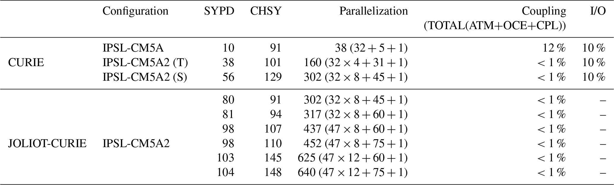
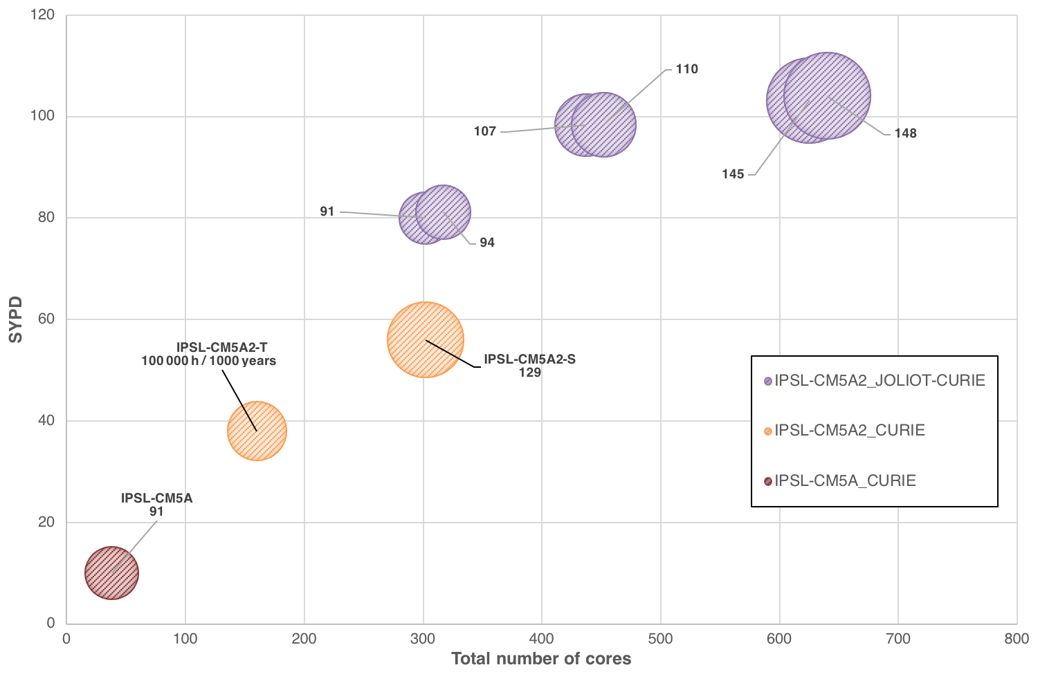
Figure A1 Scalability, i.e., SYPD as a function of parallelization, of IPSL-CM5A2 on the CURIE and JOLIOT-CURIE supercomputers. The surface area of the disks is proportional to the computing cost (core hours per simulated year; CHSY).

A2 Performance analysis

A2.1 IPSL-CM5A2 vs. IPSL-CM5A: computing performance on the CURIE supercomputer

This section assesses how the technical developments depicted in Sect. 2.2 improve the computing performance of the model. From Balaji et al. (2017), we use a set of metrics relevant for studying computational performance of IPSL-CM5A2. Besides SYPD, four metrics are used here:

• CHSY is the product of the model elapsed time for 1 simulated year multiplied by the number of computing cores. It indicates the computing cost of a simulation.

• Parallelization indicates the number of computing cores allocated for the simulation.

• Coupling cost is the overhead due to the coupling, computed as the cost of the coupling algorithm itself, i.e., the ratio of CHSY with and without coupling (CHSY – CHSY no coupling)/CHSY. “No coupling” indicates atmospheric model only.

• Data output cost is the cost of performing I/O, computed as the ratio of CHSY with and without I/O: (CHSY – CHSY no I/O)/CHSY.

Compared to IPSL-CM5A, which could be run on 38 cores only, hybrid parallelization for IPSL-CM5A2 permitted to design two configurations using more than 100 cores: a high-throughput version (IPSL-CM5A2-T) on 160 cores and a “fast” version (IPSL-CM5A2-S) running on 302 cores. IPSL-CM5A2-T configuration allows to reach 38 SYPD (3.8 times faster than IPSL-CM5A) with a 10.8 % increase in computing cost (CHSY, Table A1 and Fig. 2). IPSL-CM5A2-S reaches 56 SYPD, for a CHSY 42 % larger than for IPSL-CM5A (129 000 h for 1000 simulated years). Besides, CHSY is greater for IPSL-CM5A2-S, which means there is a better use of a resource allocation than with IPSL-CM5A. The replacement of the sequential OASIS3.3 coupler by the parallel OASIS3-MCT library in IPSL-CM5A2 also allows reducing the cost of the coupling from 12 % to 1 % of the total CPU time of a simulation. Regarding input/output aspects, IPSL-CM5A used the IOIPSL library, which performed sequential writing and imposed a rebuild post-processing step to merge multiple files into one single file. Instead, IPSL-CM5A2 uses the XIOS library that writes out data asynchronously using dedicated I/O servers. Parallel writing allows users to obtain directly one single file without any time-consuming rebuild step. Still, although the writing is performed asynchronously, the I/O cost remains important in IPSL-CM5A2 (10 %) due to operations (temporal operations, variables combinations) that are now performed by the library (on the client side, i.e., model process) rather than previously into the model.

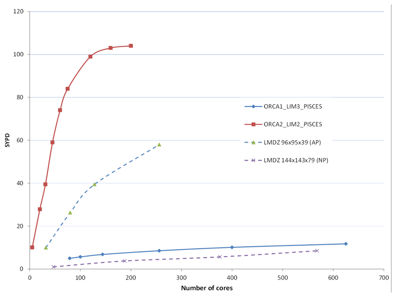
Figure A2 Computing performance for LMDZ and NEMO component at two resolutions in the early tests made on supercomputer CURIE.

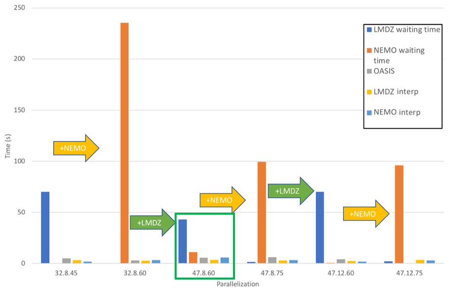
Figure A3 Waiting time of the model components and computation time of the coupler and interpolations, as a function of incremental resources provided to each component. The XX.X.X code on the x axis indicates successively the number of MPI processes, OMP threads for LMDZ and MPI processes for NEMO. This shows that most efficient configuration is the one with 47 MPI and 8 OMP dedicated to LMDZ and 60 MPI dedicated to NEMO.

Figure A4 IPSL-CM5A2 computing performance compared to IPSL-CM6-LR. Scalability, i.e., SYPD as a function of parallelization, of IPSL-CM5A2 on CURIE and JOLIOT-CURIE supercomputers compared to IPSL-CM6-LR (blue disks) on JOLIOT-CURIE. The surface area of the disks is proportional to the computing cost (CHSY).

A2.2 Performance of IPSL-CM5A2 on the JOLIOT-CURIE supercomputer

Switching from CURIE to JOLIOT-CURIE supercomputer opened opportunities to increase performance of IPSL-CM5A2 through several aspects: first, replacing Intel Sandy Bridge by more recent Intel Skylake processors was expected to reduce computation time. Second, we decided to test higher parallelization levels by combining (i) two-latitude band parallelization (instead of three), (ii) an increased number of OMP processes for LMDZ and (iii) more MPI processes for NEMO. Figure A2 depicts the scaling of IPSL-CM5A2 on JOLIOT-CURIE and CURIE. It shows that for the same parallelization set at 302 cores, IPSL-CM5A2 computes about 43 % faster on JOLIOT-CURIE than on CURIE (80 SYPD compared to 56 SYPD), with a cost reduced by ∼30 % (91 000 h for 1000 years). Finding the most valuable configuration requires both to find a trade-off between maximizing SYPD and minimizing CHSY for each component and to minimize each component waiting time in coupled configuration. To achieve the latter goal, we used LUCIA (Maisonnave and Caubel, 2014) to determine LMDZ and NEMO computing and waiting time. From the 302-core configuration, we made a step-by-step increase in LMDZ and NEMO resources that shows that both components' waiting times are minimized when LMDZ runs on 47 MPI processes and 8 OMP threads together with NEMO using 60 MPI processes (Fig. A3). This configuration uses 437 cores and allows simulating 98 years per day, leading to a cost of 107 000 h for a thousand-year simulation. Scaling up does not provide significant improvements in SYPD numbers but the cost of the simulation is dramatically enhanced (39 % increase) when we dedicate more than 600 cores to the model (Fig. A1 and Table A1). Consequently, the 437-core configuration has been chosen as the distributed version of reference.

Appendix B: Supplemental mean state diagnostics and modes of variability

This section includes supplemental diagnoses for the mean state of the historical simulation, namely a comparison of 50^∘ S–50^∘ N SST annual mean value with CMIP5 climate models (Fig. B1) and winter and summer 850 hPa wind divergence (Fig. B2), that helps explain rainfall patterns in the tropics. Detailed diagnoses of modes of variability comparing IPSL-CM5A, IPSL-CM5A2 and data are also presented.

Figure B1 Simulated SST of the historical experiment compared to results from CMIP5 models.

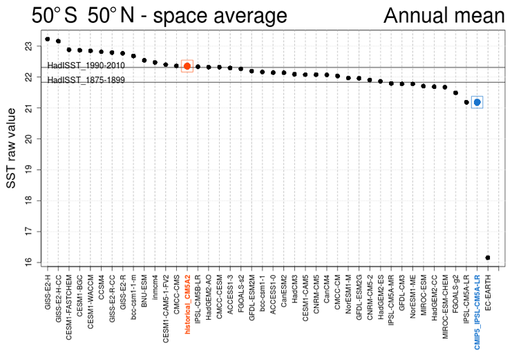
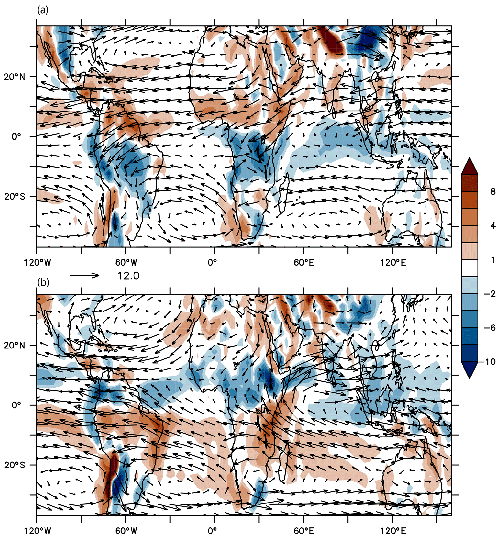
Figure B2 The 850 hPa wind (vectors) and wind divergence (10⁻⁶ s⁻¹) for DJF (a) and JJA (b).

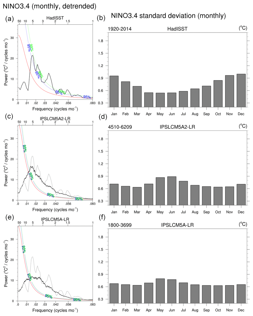
Figure B3 (a) Power spectra of the NINO3.4 index (SST in 5^∘ N–5^∘ S, 170–120^∘ W) in variance-conserving form, in observations (a, b), the Hadley Centre Sea Ice and Sea Surface Temperature dataset (HadISST, 1920–2016) and the PREIND simulations of (b) IPSL-CM5A and (c) IPSL-CM5A2. The best-fit first-order Markov red noise spectrum (red curve) and its 95 % (blue curve) and 99 % (green curve) confidence bounds are shown on each panel. (b, d, f) Monthly standard deviation of the NINO3.4 index for the same observations and simulations.

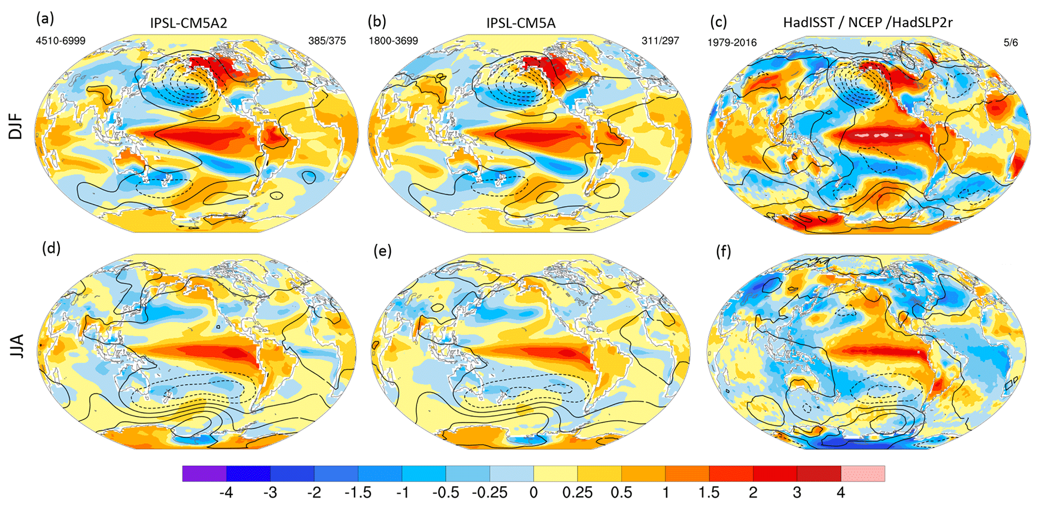
Figure B4 Composite of all years greater than 1 standard deviation (El Niño) and all years less than −1 standard deviation (La Niña), based on the December NINO3.4 index (SST in 5^∘ N–5^∘ S, 170–120^∘ W) smoothed with a three-point binomial filter, for observations (1979–2016 period) and for the PREIND simulations of (a, d) IPSL-CM5A and (b, e) IPSL-CM5A2. The number of El Niño/La Niña events composited is shown in the right subtitle. Temperatures are color shaded and in units of Celsius, and the SST in the ocean and the 2 m temperature over the continent are shown. Sea-level pressure is contoured from −16 to 16 hPa by 2 hPa; negative contours are dashed. Panels (a)–(c) indicate DJF, almost simultaneous with the December NINO3.4, while panels (d)–(f) indicate JJA preceding December NINO3.4 by about 5 months.

Figure B5 SST patterns for the PDO. The PDO is defined using the monthly leading principal component of North Pacific (20–70^∘ N, 110^∘ E $--$ 100^∘ W) area-weighted SST* anomalies, where SST* denotes that the global mean SST anomaly has been removed at each time step. The pattern is created by regressing SST anomalies (in ^∘C) onto the normalized PC time series.

Appendix C: Cretaceous supplemental analysis: equilibrium, seasonal temperatures and mixed-layer depth

This section presents simulated surface conditions for the Cretaceous after 3000 years of simulation (last 100-year average).

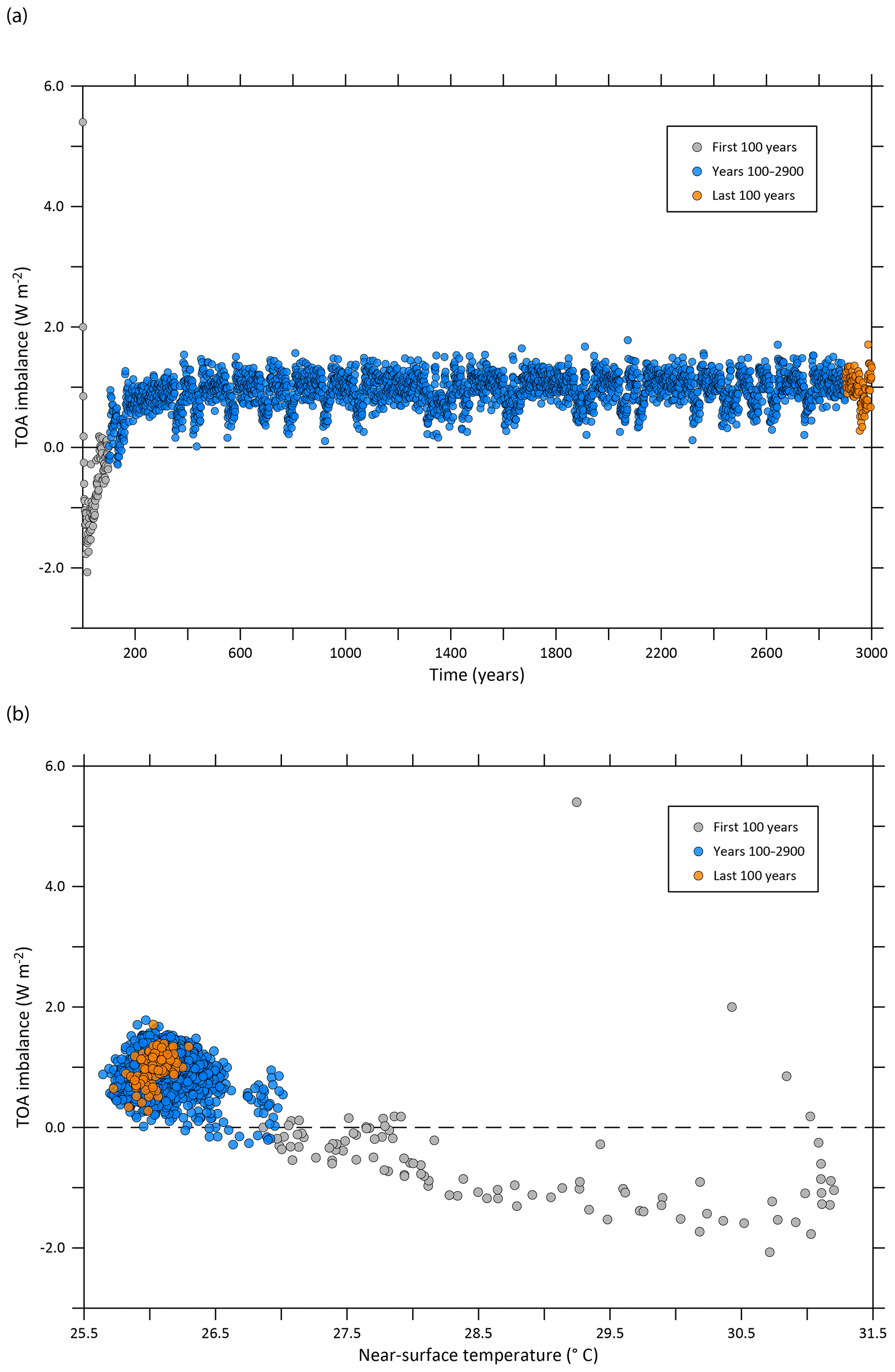
Figure C1 (a) Time series of TOA imbalance for the 3000 years of the Cretaceous simulation. (b) TOA imbalance vs. near-surface temperature.

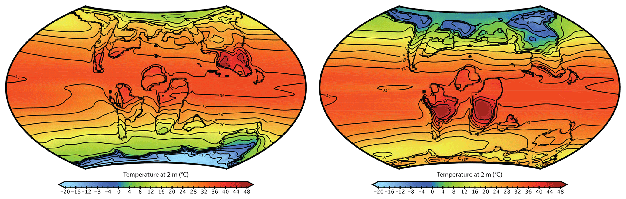
Figure C2 Simulated JAS and JFM near-surface temperature after the 3000-year run for the Cretaceous experiment.

Figure C3 Simulated JAS and JFM mixed-layer depth after the 3000-year run for the Cretaceous experiment.

Appendix D: Glossary

ACC:	Antarctica circumpolar current
AMOC:	Atlantic Meridional Overturning Circulation
AMV:	Atlantic multidecadal variability
CERES:	Clouds and the Earth's Radiant Energy System
CHSY:	core hour per simulated year
CMIP:	Coupled Model Intercomparison Project
CRF:	cloud radiative forcing
DGVM:	dynamic global vegetation model
DJF average:	December–January–February average
EBAF:	energy balanced and filled fluxes
EMIC:	Earth system model of intermediate complexity
EOF:	empirical orthogonal function
ESM:	Earth system model
GCM:	general circulation model
GPCP:	global precipitation climatology project
HPC:	high-performance computing
I/O:	input/output
IPSL:	Institut Pierre Simon Laplace
ITCZ:	Intertropical Convergence Zone
JJA average:	June–July–August average
LMD:	Laboratoire de Météorologie Dynamique
LW:	longwave
Ma:	million years
MPI:	Message Passing Interface
NH:	Northern Hemisphere
NPP:	net primary production
OHC:	ocean heat content
OMP:	OpenMP – Open Multi-Processing
PDO:	Pacific Decadal Oscillation
PE:	precipitation minus evaporation balance
PFT:	plant functional type
QTOA:	top-of-atmosphere net radiation
SH:	Southern Hemisphere
slp:	sea-level pressure
SSH:	sea-surface height
SST:	sea-surface temperature
SW:	shortwave
SYPD:	simulated years per day
t2m:	surface air (2 m) temperature
TSI:	total solar irradiance