the Creative Commons Attribution 4.0 License.
the Creative Commons Attribution 4.0 License.
 | 18 Jun 2020
Towards an objective assessment of climate multi-model ensembles – a case study: the Senegalo-Mauritanian upwelling region
Juliette Mignot
Carlos Mejia
Charles Sorror
Adama Sylla
Michel Crépon
Sylvie Thiria
Climate simulations require very complex numerical models. Unfortunately, they typically present biases due to parameterizations, choices of numerical schemes, and the complexity of many physical processes. Beyond improving the models themselves, a way to improve the performance of the modeled climate is to consider multi-model combinations. In the present study, we propose a method to select the models that yield a multi-model ensemble combination that efficiently reproduces target features of the observations. We used a neural classifier (self-organizing maps), associated with a multi-correspondence analysis to identify the models that best represent some target climate property. We can thereby determine an efficient multi-model ensemble. We illustrated the methodology with results focusing on the mean sea surface temperature seasonal cycle in the Senegalo-Mauritanian region. We compared 47 CMIP5 model configurations to available observations. The method allows us to identify a subset of CMIP5 models able to form an efficient multi-model ensemble. The future decrease in the Senegalo-Mauritanian upwelling proposed in recent studies is then revisited using this multi-model selection.
- Article
(5453 KB) - Full-text XML
- BibTeX
- EndNote


In this study, we present a methodology aimed at selecting a coherent sub-ensemble of the models involved in the Climate Model Intercomparison Project Phase 5 (CMIP5) that best represents specific observed characteristics. While the future evolution of the global climate is subject to great changes and great uncertainty (Collins et al., 2014), the most common way to predict the evolution of the climate is to run climate models that include fully coupled atmosphere–ocean–cryosphere–biosphere modules. Due to their low resolution and the fact that they use different parameterizations of the physics, use numerical schemes and sometimes include or neglect different processes, these models have some marked biases in specific regions. They also have different responses to an imposed increase in atmospheric greenhouse gases, which partly explain their mean climate biases. This variety of models allows us to assess the uncertainty of present climate representation when compared to observations and, by studying their dispersion, to roughly estimate the uncertainty of the response to future climate change.
For several generations of climate models, it has been shown that for a large variety of variables the multi-model average generally agrees better with observations of present-day climate than any single model (Lambert and Boer, 2001; Phillips and Gleckler, 2006; Reichler and Kim, 2008; Santer et al., 2009; Tebaldi and Knutti, 2007). Several studies also suggest that the most reliable climate projection is given by a multi-model averaging (Knutti et al., 2010), rather than, for example, averaging different projections performed with a single model run with different initial conditions. This result relies on the assumption that if choices of parameterizations or specific numerical schemes are made independently for each model, then the errors might at least partly compensate, resulting in a multi-model average that is more skillful than its constitutive terms (Tebaldi and Knutti, 2007). The significant gain in accuracy can be explained by the fact that the errors specific to each model compensate each other in the averaging procedure used to build the multi-model mean. However, the number of general circulation models (GCMs) available for climate change projections is increasing rapidly. For example, the CMIP5 archive (Taylor et al., 2012), which was used for the fifth IPCC Assessment Report (Stocker et al., 2013), contains outputs from 61 different GCMs, and 70 contributions are expected for CMIP6. It thus becomes possible – and probably necessary – to select and/or weight the models constituting such an average. Recent work has suggested that weighting the multi-model averaging procedure could help to reduce the spread and thus uncertainty of future projections. Such an approach has been applied extensively to the issue of climate sensitivity (Fasullo and Trenberth, 2012; Gordon et al., 2013; Huber and Knutti, 2012; Tan et al., 2016). Valuable improvement of model selection has also been found in studies of the carbon cycle (Cox et al., 2013; Wenzel et al., 2014), the hydrological cycle (Deangelis et al., 2015; O'Gorman et al., 2012), the Antarctic atmospheric circulation (Son et al., 2010; Wenzel et al., 2016), extratropical atmospheric rivers (Gao et al., 2016), atmospheric and ocean heat transports (Loeb et al., 2015), European temperature variability (Stegehuis et al., 2013) and temperature extremes (Borodina et al., 2017).
The present paper works towards the elaboration of an objective method to select models according to their performance for a specific phenomenon. Here, we use the Senegalo-Mauritanian upwelling area as a case study to construct an efficient climate multi-model combination together with its related confidence interval in order to anticipate the effect of climate warming by the end of the century in this region. The Senegalo-Mauritanian upwelling has been the focus of increasing attention over recent years. The very productive waters associated with the upwelling have a strong economic impact on fisheries in Senegal and Mauritania and a crucial societal importance for local populations. It is therefore important to predict the evolution of the dynamics and the physics of the upwelling in the forthcoming decades, due to the effect of climate warming and its consequences for biological productivity, which may impact the fisheries. The Senegalo-Mauritanian upwelling lies at the southern end of the Canarian upwelling system, which has a relatively weak seasonality and is maximum in summer. By contrast, the Senegalo-Mauritanian upwelling presents a well-marked seasonal variability. Its intensity is stronger in boreal winter, and it disappears in summer with the northward progression of the intertropical convergence zone (ITCZ). Due to the enrichment of the sea surface layers with nutrients upwelled from deep layers, it drives an important phytoplankton bloom that is observed on ocean color satellite images (Demarcq and Faure, 2000; Farikou et al., 2015). The maximum intensity of this bloom occurs in March–April (Farikou et al., 2015; Faye et al., 2015; Ndoye et al., 2014). Its important seasonal cycle is also associated with mesoscale patterns whose variability has been recently studied by several oceanographic campaigns (Capet et al., 2017; Faye et al., 2015; Ndoye et al., 2014) and theoretical work (Sirven et al., 2019). Sylla et al. (2019) have recently shown that the intensity of the sea surface temperature (SST) seasonal cycle along the coasts of Senegal and Mauritania was a good marker of the upwelling in this specific region in climate models. They have used this index together with other more dynamical indices to predict that the upwelling will decrease by about 10 % of its present-day amplitude by the end of the 21st century. Nevertheless, their study also highlighted a large uncertainty due to model biases in this region. The method we have developed selects a subset of the CMIP5 ensemble based on the capability of the climate models to reproduce the SST seasonal cycle observed during the historical period in key sub-regions. These sub-regions are identified by a neural classifier. The method leads us to rank the different models and to determine an efficient multi-model combination for the analysis of the Senegalo-Mauritanian upwelling and projections of its behavior in global warming conditions.
The paper is structured as follows: Sect. 2 presents the different climate models and the climatological observations used in the study, together with the region of interest. The classification method is described in Sect. 3 and applied to the extended region. Section 4 presents a qualitative analysis able to group the different climate models into clusters presenting similar performances. Section 5 investigates the results of the method applied over a smaller area, more focused over the upwelling region. Section 6 uses the two multi-model clusters defined in Sects. 4 and 5, respectively, to tentatively predict the representation of the Senegalo-Mauritanian upwelling changes under global warming. Conclusions are given in Sect. 7.
2.1 Data
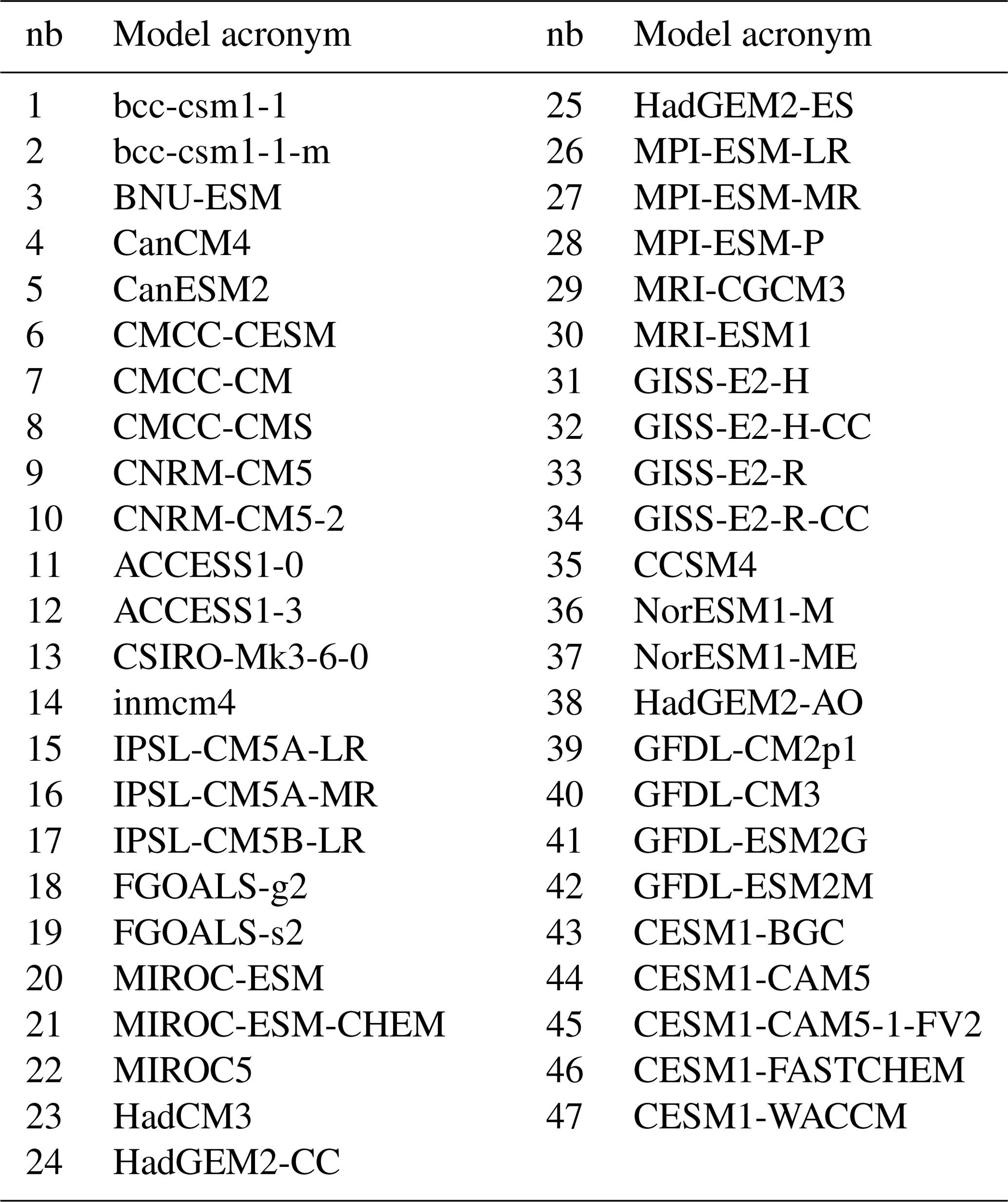
This study is based on the CMIP5 (Coupled Model Inter-comparison Project Phase 5) database. We use the output of 47 simulations listed in Table 1. The models are evaluated over the historical period defined as [1975–2005] by comparing their output to observations. The mean seasonal cycle of SST anomalies over this period is constructed for each model grid point as the difference between the monthly mean temperature and the mean annual temperature. When several members of historical simulations are available for a specific model configuration, they are averaged together. However, this has practically no impact on the estimated mean seasonal cycle (not shown). The mean climatological cycle of the CMIP5 models under study is evaluated against the Extended Reconstructed Sea Surface Temperature data set (ERSST-v3b, Smith et al., 2008), averaged over the same time period. This data set was produced by NOAA at 2∘ spatial resolution. It is derived from the International Comprehensive Ocean–Atmosphere Dataset with missing data filled in by statistical methods. This data set is used as the target to be reproduced and is denoted “observation field” hereafter. In order to deal with data at the same resolution, all model outputs as well as the observation fields were regridded on a 1∘ resolution regular grid prior to analysis. A previous study (Sylla et al., 2019) has compared the performance of this data set as compared to the gridded SST data set from the Met Office Hadley Centre HadISST (Rayner, 2003). The main results regarding the future of the upwelling were shown to be independent of the validation data set, primarily because the models' biases and the inter-model differences were much larger than the differences between the validation data sets. The methodological and oceanographic results presented in this study are thus expected to depend only very weakly on the target data set.
Table 1List of the CMIP5 models used for the comparison. The reader is referred to the CMIP5 documentation for more information on each of them. Here, each configuration is furthermore given a number, for easier identification in subsequent figures.
In Sect. 6, the model selections are used to characterize the response of the upwelling to climate change. This response is characterized in terms of SST anomalies as well as wind intensity. For wind intensity, the simulated wind stress is compared to the TropFlux reanalysis. This data set combines the ERA-Interim reanalysis for turbulent and longwave fluxes and ISCCP (International Satellite Cloud Climatology Project) surface radiation data for shortwave fluxes. This wind stress product is described and evaluated in Praveen Kumar et al. (2011).
2.2 The Senegalo-Mauritanian upwelling region
In this study, we evaluate the ability of the different climate models to represent the Senegalo-Mauritanian upwelling. Following Sylla et al. (2019), we consider the intensity of the seasonal cycle of the SST anomaly to be a marker of the upwelling variability and localization. This variable is shown in Fig. 1 for the eastern tropical Atlantic. This figure confirms that the Senegalo-Mauritanian coast stands out with a very strong seasonal SST cycle as compared to similar latitudes in the open ocean. This results from the cold SST generated by the strong winds occurring in winter. The Senegalo-Mauritanian upwelling is confined in a small region on the order of 100 km off the western coast of Africa. It is part of a complex and fine-scale regional circulation system recently revisited by Kounta et al. (2018). Since the grid mesh of most of the climate models is on the order of 1∘ (∼100 km), this regional circulation is poorly resolved, which favors a relatively large-scale analysis of the upwelling representation in climate models. The Senegalo-Mauritanian upwelling is also embedded in a large-scale oceanic circulation pattern, encompassing the North Equatorial Counter Current flowing eastward in the southern part of the region and the return branch of the subtropical gyre in the northwestern part. Therefore, we firstly study the representation of the SST seasonal cycle intensity in the different climate models over a relatively large region that includes part of the Canary Current in the north and the Guinea Dome in the south. The so-called “extended region” is defined by a rectangular box extending from 9 to 45∘ W and from 5 to 30∘ N (Fig. 1). In a second step, we will proceed to the same analysis and classification of the models within a much more focused (hereafter zoomed) region, namely [16–28∘ W and 10–23∘ N] (Fig. 1). All the results below will be first shown for the extended region. Comparison with the focused region will be done in Sect. 4.

Figure 1Amplitude of the SST seasonal anomalies in the western tropical North Atlantic. SST data are from the ERSSTv3b data set averaged between 1975 and 2005. The two black boxes show the extended and zoomed regions, respectively, on which the statistical classifications were performed (see text for details).
The methodology we have developed is based on the ability of the climate models to adequately reproduce the climatology of the seasonal cycle of the SST anomalies as observed during the last 3 decades in key sub-regions of the studied domain. These key sub-regions are determined from the similarity of their physical and statistical characteristics through an unsupervised classification, which clusters pixels with similar observed seasonal SST climatology. We chose to deal with a neural classifier, the so-called self-organizing map (SOM hereafter) developed by Kohonen (2013), followed by a hierarchical ascendant clustering (HAC, Jain and Dubes, 1998). This method leads to a dynamically interpretable classification. The SOM determines a vector quantization of the data set, which compresses the initial data set into a relatively small number of reference vectors. Doing so allows us to take the nonlinearities of the data set into account and to filter the noise, which can make the classification spurious. This reduced number of dataset vectors enables an HAC to determine the highly nonlinear borders between the different SOM clusters. This procedure has been used with success in several studies (Farikou et al., 2015; Jouini et al., 2016; Niang et al., 2003, 2006; Sawadogo et al., 2009). Note that the use of an HAC directly on the initial data set would not be efficient in the present study because the number of degrees of freedom (here the grid points of the initial domain) is too large for this method to work efficiently. In the present section, we describe the methodology we developed to score the different climate models with respect to the observations. In Sect. 4, we will tentatively group the different climate models into blocks with the same behavior by using a multiple correspondence analysis (MCA).
3.1 The unsupervised classification method
The first step of the methodology was to decompose the selected region into different classes (the key sub-regions mentioned above) by using a neural network classifier, the so-called SOM (Kohonen, 2013). This algorithm constitutes a powerful nonlinear unsupervised classification method. It has been commonly used to solve environmental problems (Hewitson and Crane, 2002; Jouini et al., 2013, 2016; Liu et al., 2006; Reusch et al., 2007; Richardson et al., 2003). The SOM aims at clustering vectors (here the 12 SST seasonal anomalies) of a multidimensional database (D) (here the grid points of the studied domain) into classes represented by a fixed network of neurons (the SOM). The SOM is defined as an undirected graph, usually a two-dimensional rectangular grid. This graphical structure is used to define a discrete distance (denoted by δ) between the neurons of the map and thereby identify the shortest path between two neurons. Moreover, the SOM enables the partition of D in which each cluster is associated with a neuron of the map and is represented by a prototype that is a synthetic multidimensional vector (the referent vector w). Each vector z of D is assigned to the neuron whose referent w is the closest, in the sense of the Euclidean norm (EN), and is called the projection of the vector z onto the map. A fundamental property of a SOM is the topological ordering provided at the end of the clustering phase: two neurons that are close on the map represent data that are close in the data space. In other words, the neurons are gathered in such a way that if two vectors of D are projected onto two “relatively” close neurons (with respect to δ) on the map, they are similar and share the same properties. The estimation of the referent vectors w of a SOM and the topological order is achieved through a minimization process using a learning dataset base, here from the observations. The cost function to be minimized is of the form
where c∈SOM indices the neurons of the SOM, χ is the allocation function that assigns each element zi of D to its referent vector and δ(cχ(zi)) is the discrete distance on the SOM between a neuron c and the neuron allocated to observation zi. KT a kernel function parameterized by T (where T stands for “temperature” in the scientific literature dedicated to SOM) that weights the discrete distance on the map and decreases during the minimization process. At the end of the learning process, the classification can be visualized onto the SOM and interpreted in terms of geophysics.
3.2 Classification of the observations
In the present problem we chose to classify the annual cycles of the SST seasonal anomalies observed in the Senegalo-Mauritanian upwelling. The study was made on the “extended region” constituted of pixels, but this enlarged region covers a part of the African continent, and 157 pixels are in fact over land. That means that we have truly 743 ocean pixels to deal with. We consider a time period of 30 years [1975 to 2005] extracted from the ERSST-V3b database. For a given grid point and a given year and month, the monthly anomaly is the SST of the pixel for which we have subtracted the mean of the considered year. The climatological mean of the anomaly is then computed for each grid point by averaging each climatological month over the 30 years. Thus, the learning data set D is a set of 743 12-component vectors z, each component being the mean monthly anomaly computed as above. We denote as “SST seasonal cycle” the vector z in the following.
We used a SOM to summarize the different SST seasonal cycles present in the “extended region”. We found that 120 prototypes (or neurons) can accurately represent the 743 vectors of D. This reduction (or vector quantization) is made by using a rectangular SOM of 30×4 neurons.
We then reduced the number of neurons in order to facilitate their interpretation in terms of geophysical processes. For this, we applied a HAC using the Ward dissimilarity (Jain and Dubes, 1988). We grouped the 120 neurons of the SOM into a hierarchy that can contain between 1 and 120 clusters. Then the different classifications proposed by the HAC were applied to the geographical region: each SST seasonal cycle of each grid point of the region is assigned to a neuron and consequently to a cluster (assignment process), thereby defining the so-called region clusters. The problem is then to choose a number of clusters that adequately synthesizes the geophysical phenomena over the region. This was done by looking at the different possible classifications and choosing one representing the major characteristics of the upwelling region. In Fig. 2a, we observe that when we partition the SOM into seven clusters, the associated seven region clusters are constituted of contiguous pixels in the geographic map and that two clusters (6, 7) are within the upwelling region and present a well-marked seasonal cycle. For each region cluster, we estimated the monthly mean of the SST seasonal cycle and the associated spread captured by the neurons constituting this region cluster.
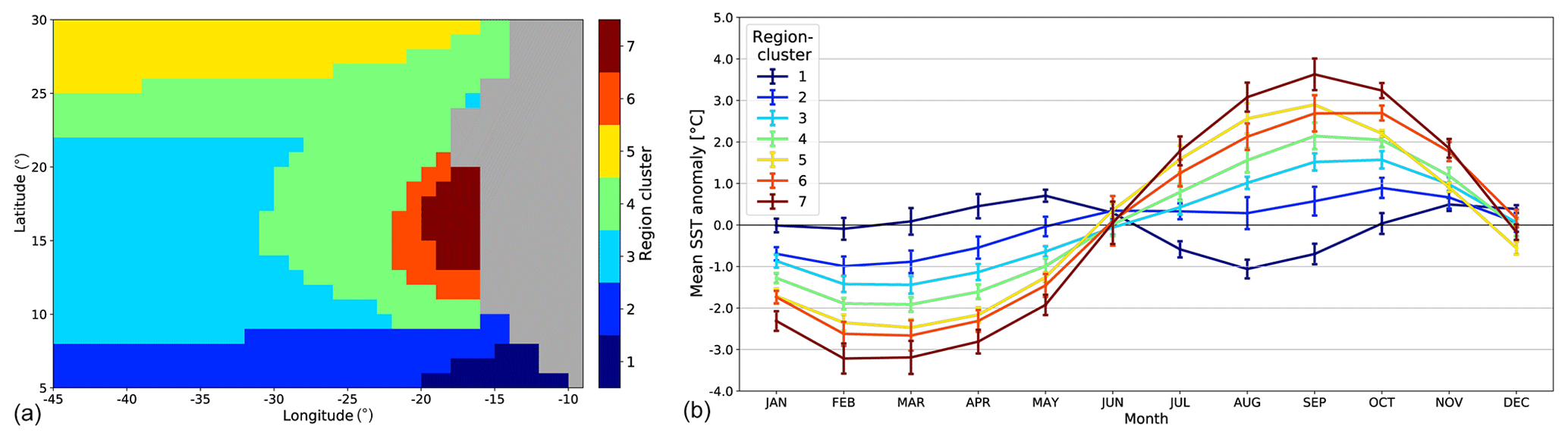
Figure 2(a) Region clusters associated with the SOM clusters obtained after a HAC on a 30×4-neuron SOM learned on ERSSTv3b observations in the extended zone (see text for details). (b) Ensemble-mean monthly climatological SST anomalies for the grid points of the seven region clusters. The error bars show the standard deviation of this ensemble mean.
The typical SST climatological cycles for each region cluster are presented in Fig. 2b together with their related error bars. We note that the region clusters are well identified, their typical climatological annual cycles of SST being well separated. Furthermore, the seven region clusters are spatially coherent and have a definite geophysical significance.
For the extended region under study, 7 therefore appears to be an adequate cluster number, since this number balances a clear partition of the clusters on the HAC decision tree with a clear physical significance to each region cluster. The Senegalo-Mauritanian coastal upwelling is associated with clusters 7 and 6. Cluster 2 corresponds to deep tropical waters associated with the equatorial countercurrent. Cluster 1 corresponds to surface waters of the Gulf of Guinea. Cluster 3 corresponds to the offshore tropical Atlantic, and cluster 5 has extratropical characteristics. Cluster 4 is a transition between 3 and 5. As expected, the equatorial regions (clusters 1 and 2) have a very weak seasonal cycle, which increases towards the extratropics (clusters 3 to 5). The upwelling regions (clusters 6 and 7) are characterized by an exceptionally strong seasonal variability.
3.3 Classification of the climate models on the extended upwelling region
The aim is now to find the model(s) that best fit the “observation field”. A heuristic manner is to compare the pattern of the different region clusters of the CMIP5 models with respect to those of the “observation field” through a sight-evaluating process. This kind of approach has been proposed in Sylla et al. (2019), and we indeed immediately see that some models better fit the “observation field” than others. Nonetheless, this method remains very subjective.
In the following, we present a more objective approach. We use the previous classification to objectively estimate how each CMIP5 model fits the “observation field” and its seven region clusters. For this, we projected the SST annual cycle of each CMIP5 model grid point of the extended region onto the SOM learned with the observations (Sect. 3.2) using the assignment procedure described in this section. Each grid point thus corresponds to a cluster of the SOM and is represented on the geographical map by its corresponding color. Doing so, we can represent each CMIP5 model by the geographical pattern of the seven clusters partitioning the SST seasonal cycle of its grid points. The geographical maps representing the 47 models and their associated clusters are plotted in Fig. 3. This graphical visualization is easier to compare than the original characteristics (amplitude and phase) of the annual cycle at each grid point of a model since each grid point can only take one discrete value among seven. This representation immediately allows identification of the model biases and the models that best reproduce the cluster regions identified in the observations. A huge amount of information could in principle be extracted from these maps, both from individual modeling groups, to understand the representation of this region by the models and the origins of possible biases, and from experts of the area, to understand the difficulties of the climate models in representing the SST seasonal cycle in this region.

Figure 3Projection of the 47 climate models of the CMIP5 database onto the SOM learned with ERSSTv3b climatology in the extended zone (see Fig. 1). On top of each panel, we figure the number referencing the model, its name (Table 1), and its skill given as a mean percentage (see text). The models are ordered according to their skill in decreasing order. The seven region clusters (or SOM clusters) are defined by applying an HAC to the SOM output learned with the observation field. They are represented by different colors. The numbers in the color bar on the right of each panel represent the skill for each region cluster. The observation field is shown in the bottom right panel and the numbers in front of the color bar reference the region cluster.
For a more quantitative assessment, we counted the number of grid points of a region cluster for a given CMIP5 model matching the same region cluster of the “observation field”. We then computed the ratio between that matching number and the number of pixels of the region cluster of the considered model. That number is noted in the color bar for each region cluster in Fig. 3. We denote Rm,i the ratio for the region cluster i and the model m, where is the number of the region cluster and is the number of the model (see Table 1). We note that Rm,i ≤1. Doing so, each model m is represented by a seven-dimensional vector Rm, each component being the ratio of a region cluster. We estimated the total skill of a model by averaging the seven ratios. Note that this procedure gives the same weight to each region cluster whatever its number of grid points and its proximity to the upwelling region. In the following, the skill is presented as a percentage: the higher the skill, the better the fit. In Fig. 3, the 47 CMIP5 models are ranked by their total skill, which is indicated above each panel beside the model name. The model skills are very diverse, ranging from 79 % to 28 %. This figure also shows that the models presenting the best total skill are also those representing thoroughly the upwelling region. Some models represent the large-scale structure in the eastern tropical Atlantic (Region-clusters 3, 4, and 5) very well, but not the upwelling (33-GISS-E2-R and 34-GISS-E2-R-CC, for example). Others represent pretty well the upwelling region clusters (Region-clusters 6 and 7), but not the large-scale structures of the SST seasonality (13-CSIRO-Mk-3-6-0 and 6-CMCC-CESM, for example). None of these models is ranked among the best models, with a score greater than 60 %. As indicated above, this representation gives a very synthetic view of the structure of the seasonality of the SST cycle in each of the models, potentially a very useful guide for climate modelers to identify rapidly major biases.
In order to further progress in the selection of the models, the 47 climate models and the observation field were then analyzed by using an MCA. MCA is a multivariate statistical technique that is conceptually similar to principal component analysis (PCA) but applies to categorical rather than continuous data. Similarly to PCA, it provides a way of displaying a set of data in a two-dimensional graphical form.
In the following, we apply a MCA to the (47,7) matrix R= [Rm,i] whose elements represent the skills of the clusters of the models shown in front of the color bars in Fig. 3: the rows m represent the 47 different models, the columns i the seven region clusters. The MCA, like the PCA, projects the initial matrix onto a new basis in such a way that the new axes are the matrix eigenvectors (PC), the inertia of each axis being the corresponding eigenvalues. According to the theory, the MCA matrix analysis of R gives independent PCs. Each model is thus now associated with a six-dimensional vector on which it has a specific weight. The MCA uses for this analysis the χ2 distance. In Fig. 4, we present the projection of the models and the “region clusters” in the plane formed by the two first axes (x= PC1 and y= PC2) of the MCA. These two axes represent 70 % of the total inertia. Each model is represented by a small circle and each region cluster by a purple square. We also projected the observation field (green diamond) onto that plane. To have a more precise view of the topology, it would be necessary to consider the projection onto the five other PCs, which represent 30 % of the inertia.
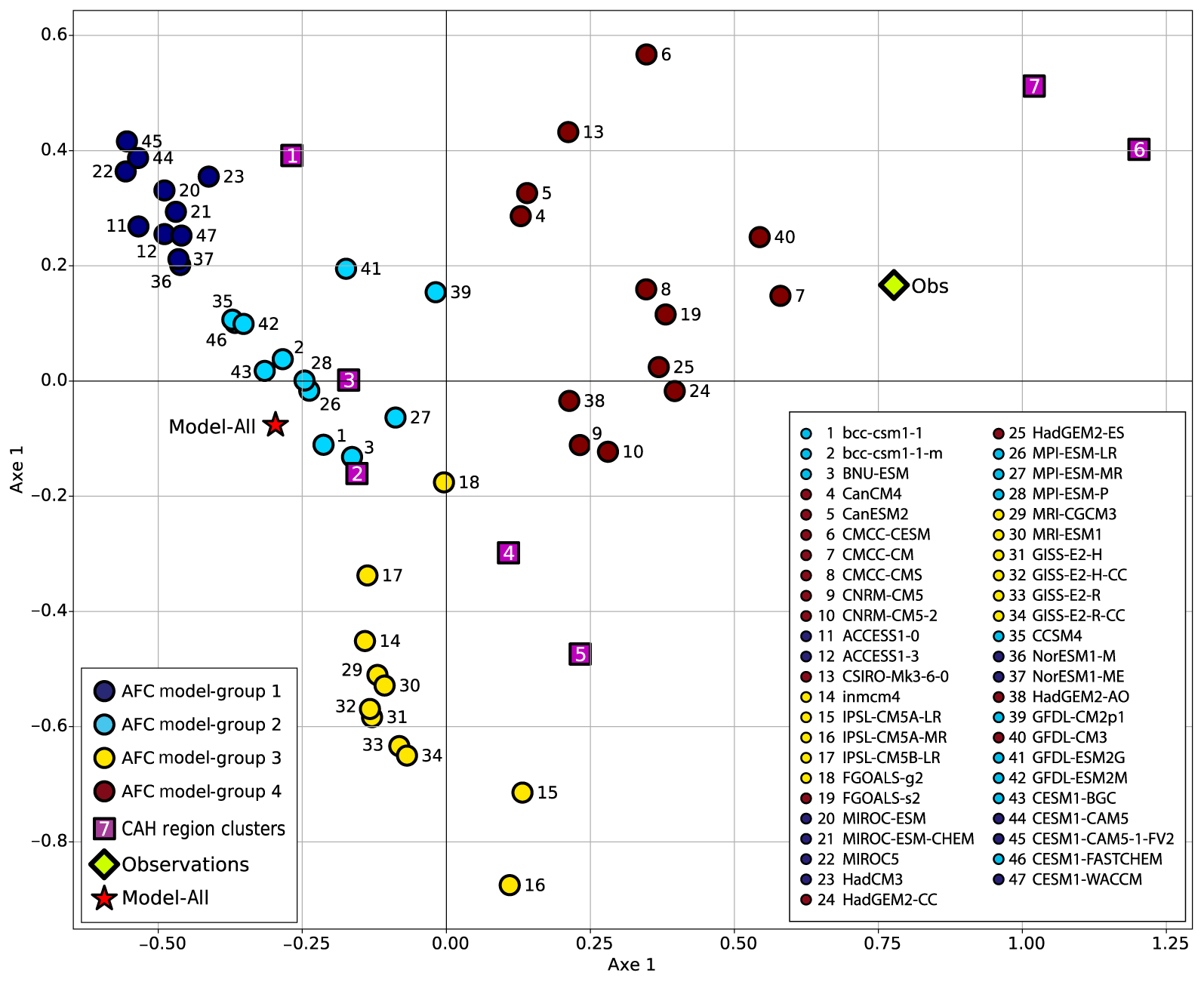
Figure 4Projection of the CMIP5 models (colored circles) and the observation field (green diamond) defined by their cluster skill vectors onto the first two axes of the MCA. The seven region clusters of the observation field are represented by purple squares. The colors of the circles denote the four groups of models obtained after an HAC was performed on the seven MCA components of the models. The projection of the full multi-model mean (47 models) is represented by a red star. We note that some bias can be introduced into this projection since the projection onto the other axes can be of importance.
In the (PC1, PC2) plane, the shorter the distance between two models, the more similar the distribution of their region-cluster skills. Proximity between a model and a region cluster leads us to affirm that this region cluster is well represented by that model. Clearly, some models adequately represent the southern part of the extended region (Region-clusters 1, 2 or 3), where the SST seasonal cycle is weak, and are very distant from the upwelling regions (Region-cluster 6 and Region-cluster 7) whose large SST cycle is poorly reproduced. In this group of models, one recognizes the model 16-IPSL-CM5A-MR, at the extreme bottom of Fig. 4, close to Region-clusters 4 and 5, consistently with Fig. 3. At the other end of this group of models, model 23-HadCM3 for example is located very close to Region-cluster 1. Figure 3 indeed shows that most of its grid points over the region of interest have a seasonal cycle resembling the one found in the offshore tropical ocean. Another group of models is located in the center of this plan, thus at an optimal distance of each of the observed region clusters, and not far from the overall position of the observations (diamond). We recognize in this group of models those that have a high skill in Fig. 3. The positioning of the observations (green diamond in Fig. 4) with respect to the models indeed allows selection of those that best represent the observation field. The representation given in Fig. 4 allows understanding of the drawback of the different models with respect to the seven modes of SST cycles.
As indicated in the introduction, the main objective of the methodology is to select an ensemble of models that represents at best the upwelling behavior with respect to the observations and to use this ensemble to predict the impact of climate change on the Senegalo-Mauritanian upwelling with some confidence. The problem is now to determine a subset of models which has a better skill than Model-All, in other words minimize the distance to the observations. As the number of models is small enough, we chose to cluster them by an HAC according to their projections onto the six axes provided by the MCA and select the optimal jump in the hierarchical tree (Jain and Dubes, 1988). We recall that the HAC (hierarchical ascending clustering) is a bottom–up algorithm for dataset clustering. The key operation in hierarchical bottom–up clustering is to repeatedly combine the two nearest (according to a certain distance) clusters into a larger cluster. The HAC starts from individuals and combines them according to their similarity (with respect to the chosen distance) to obtain new clusters. The process is repeated up to get one cluster only (the full data set). This algorithm is visualized through a tree-like diagram, the so-called connection tree or dendrogram: the branches of the connection tree represent the connections between the clusters (Fig. 5). From Fig. 5, we obtain four homogeneous groups which are well separated (group 1, 2, 3, and 4). They are plotted with different colors in Fig. 4. We denote as Model-group 1, Model-group 2, Model-group 3, and Model-group 4 these multi-model ensembles hereafter. Note that Fig. 4 shows the projection of the individual models onto the first two axes of the MCA. The fact that only two axes are shown here can introduce some bias into the visualization, and this figure must be considered with some caution.
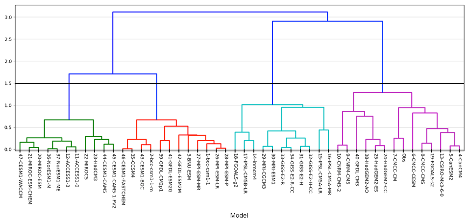
Figure 5HAC dendrogram. The horizontal line displays the 47 CMIP5 models, each model being associated with its seven-component skill vector. As the dendrogram represents a hierarchy of clusters, the numbers on the y axis give the distance between two clusters. We note an optimal “jump” on this graph: the level 1.5 on the vertical axis (materialized by a horizontal black line) is associated with four well-separated clusters corresponding to four model groups that are very different.
Through MCA+HAC, we thus grouped the models into clusters, using the χ2 distance, according to their proximity to the observations and their internal similarity. For each group, we computed a multi-model average whose outputs are the mean of the outputs of its different members, and we analyzed it according to the same procedure (projection of the SST seasonal cycle and assignment to a region cluster) used for each individual model. In addition, we introduced the full multi-model average (Model-All in the following), which is the multi-model ensemble, which averages the 47 CMIP5 model outputs. Model-All was also projected in the MCA plane, and it is represented by a red star in Fig. 4. Comparison of the four model groups with Model-All and the observations are presented in Fig. 6. This figure visually highlights the dominance of Model-group 4 for the reconstruction of the SST seasonal cycles of the different region clusters for the extended region. This is particularly clear for Region-clusters 6 and 7, which are those located in the upwelling region (Fig. 2). Model-group 3 seems to group models characterized by an equatorward shift of the main structures, since Region-cluster 1 of tropical waters is not reproduced and Region-clusters 4 and 5 of extratropical waters are overestimated. Figure 4 indeed shows that this model group is very close to Region-clusters 4 and 5, which correspond to the extratropical and transition geographical regions. Model-group 2 misrepresents the region of the Canary upwelling. Model-group 1 overestimates the SST seasonal cycle in all the tropical open Atlantic. These two last model groups overestimate Region-cluster 1, again consistently with their position in Fig. 4. A detailed physical interpretation of the model groups is nevertheless beyond the scope of this paper. Clearly Model-All represents the SST seasonal cycle of the offshore ocean, but it proposes a very poor representation of the upwelling region.
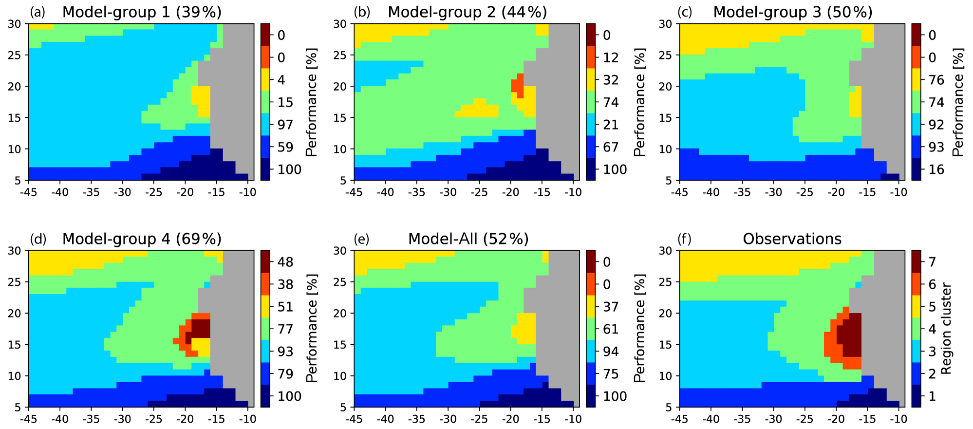
Figure 6(a–d) Projection of the multi-model ensembles (model group) onto the SOM learned with ERSSTv3b climatology in the extended zone. Multi-model ensemble performances are obtained by averaging the skill of the models forming each group. The performances are given on top of each panel. The region clusters determined by processing the observations in the extended area and their associated colors are given in panel (f). The color bars at the right of each multi-ensemble panel represent the skill (in %) associated with each region cluster. Panel (e) shows the projection for the full multi-model ensemble. Panel (f) reproduces the region clusters based on the observations also shown in Fig. 2.
Two models (models 7 and 25) have a better skill than Model-group 4 and Model-All. These two models are very close to the observations on the first two axes of the MCA (Fig. 4). It is easily seen that Model-group 4 and the projection of Model-All onto this plane are farther than that of model 7 and model 25 from the observation projection. This explains the lower performance of these two multi-models as compared to models 7 and 25. In the present case, the method permits one to determine the best models (model 7 and model 25) and to outline the best multi-model (Model-group 4) whose skill is better than any model with a probability of 95 % (number of models whose skill is smaller than the skill of Model-group 4 with respect to the total number of models). Projection of the models onto the other planes of the MCA should confirm this interpretation. One could then question the use of Model-group 4 rather than model 7 or model 25 individually. Furthermore, we argue that multi-model averages are in general more robust for climate studies than the use of a single model that can have good performance for a very specific set of constraints but not for neighboring ones. The following section will partly justify this point.
The classification presented above relies largely on the ability of the models to represent the offshore seasonal cycle of the SST. In the following, we propose to test the classification over a much more reduced area in order to focus the analysis on the upwelling area. This “zoomed upwelling region” is shown in Fig. 1.
As for the extended region, we partitioned the observations of the zoomed upwelling region with a SOM (ZSOM in the following) followed by a HAC. We then applied a new MCA to regroup the climate models. We did a similar analysis to that performed in Sect. 4. We obtained four new well-separated region clusters denoted ZRegion clusters. Figure 7 shows the four ZRegion clusters obtained from ERSSTv3b observations together with their associated mean SST seasonal cycle. Again, the ZRegion clusters are spatially coherent. The upwelling area is now decomposed into three ZRegion clusters (ZRegion-clusters 2, 3, and 4). This new decomposition thus refines the study performed for the extended region: ZRegion-cluster 1 represents the offshore ocean; its grid points typically have a SST seasonal cycle amplitude of 4 ∘C, very similar to Region-cluster 4 in the classification performed over the extended region (Fig. 2). ZRegion-cluster 4 identifies the core of the Senegalo-Mauritanian region, with grid points characterized by the greatest amplitude of the SST seasonal cycle of the domain, typically 6.5 ∘C. It is interesting to note that an additional upwelling ZRegion cluster (ZRegion-cluster 3) appears south of ZRegion-cluster 4. Indeed, several studies have shown that the Cape Verde peninsula, located around 15∘ N, separates the upwelling region into two distinct areas with a different behavior north and south of this peninsula (Sirven et al., 2019; Sylla et al., 2019). The location of the separation between ZRegion-clusters 3 and 4 is determined with some uncertainty due to the coarse resolution (1∘) of the ocean models. ZRegion-cluster 3 is marked by a time shift of the seasonal cycle: the warmest season seems to occur approximately 1 month earlier than in the other regions, as clearly seen in Fig. 7a (yellow curve in June). Due to a classification using a much larger region, such a characteristic does not appear in the extended area study. The physical interpretation of the SST seasonal cycle of this ZRegion cluster is beyond the scope of the present study, but one can suspect a role of the ITCZ seasonal migration covering these grid points earlier than further north. Finally, ZRegion-cluster 2 is a transition between the large-scale ocean and the upwelling region.
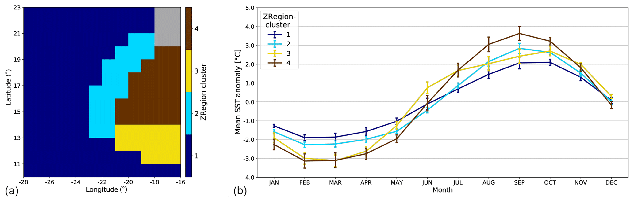
Figure 7(a) ZRegion clusters associated with the ZSOM clusters obtained after a HAC on a 10×12-neuron SOM learned on ERSSTv3b observations in the zoomed zone (see text for details). (b) Ensemble-mean monthly climatological SST anomalies for the grid points of the four ZRegion clusters. The error bars show the standard deviation of this ensemble mean.
As for the extended region, we applied a MCA to the (47×4) matrix R= [Rm,i] whose elements represent the skills of the four clusters (i) of the 47 models. This MCA was followed by a HAC leading the definition of five ZModel groups. The members of each group are given in the Appendix. Figure 8 shows the ZRegion cluster obtained in the zoomed area by projecting these five ZModel groups and Model-All onto the ZSOM and their associated performances. ZModel-group 1 is the worst performing one: only 25 % of the grid cells fall into the same class as for the observations. The structure of this model group shows that it is characterized by a homogeneous amplitude of the seasonal cycle over the whole domain, suggesting a largely reduced upwelling: only one grid point at the coast has an enhanced SST seasonal cycle as compared to the large-scale tropical ocean. ZModel-group 2 is the best performing one: 66 % of the grid points are assigned to the correct class and the general picture indeed represents a four-class picture fairly consistent with the observed structure (Fig. 7). Important biases yet remain. In particular, ZRegion-clusters 2 and 4 characterizing the upwelling extend too far offshore. The three other ZModel groups are intermediate. A relatively reduced upwelling area, with an underestimated SST seasonal cycle, characterizes ZModel-groups 3 and 4. ZModel-group 5 corresponds to a shift of the upwelling region towards the north. Model-All also shows a strongly reduced seasonal cycle, with a large number of pixels in the intermediate ZRegion-cluster 3 and very few in ZRegion-cluster 4. ZRegion cluster 3, representing the southern part of the Senegalo-Mauritanian upwelling, does not appear in the pattern of Model-All.
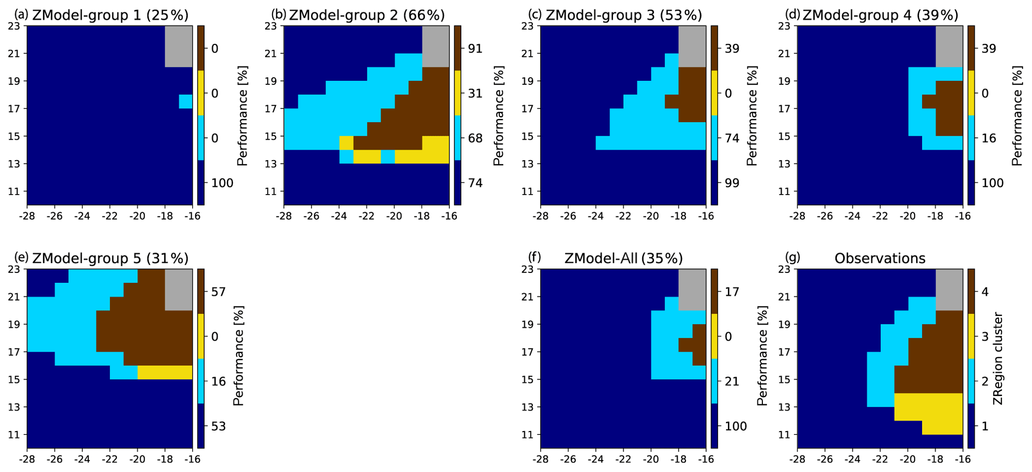
Figure 8(a–e) Projection of the multi-model ensembles (ZModel groups) onto the ZSOM. The performances are given on top of each panel. The ZRegion clusters determined by processing the observations in the zoomed region and their associated colors are given in panel (g). The color bars at the right of each multi-ensemble panel represent the skill (in %) associated with each ZRegion cluster. Panel (f) shows the same for the full multi-model ensemble. Panel (g) reproduces the region clusters based on the observations also shown in Fig. 6.
It is notable that all the models forming ZModel-group 2 are included in Model-group 4. For a more precise assessment, we can also project the entire Model-group 4, identified as the best multi-model ensemble over the extended region, onto the ZSOM (Fig. 9b). We notice that the performance of Model-group 4 remains high on this projection, indicating some robustness of this multi-model ensemble. Moreover, this ensemble now outperforms the single best model identified over the extended region (Fig. 9a). This result gives further confidence in the use of multi-model averages, illustrating that one single model can be very skillful over a specific region or for a specific analysis, but multi-model averages are more robust across various analyses and/or regions.
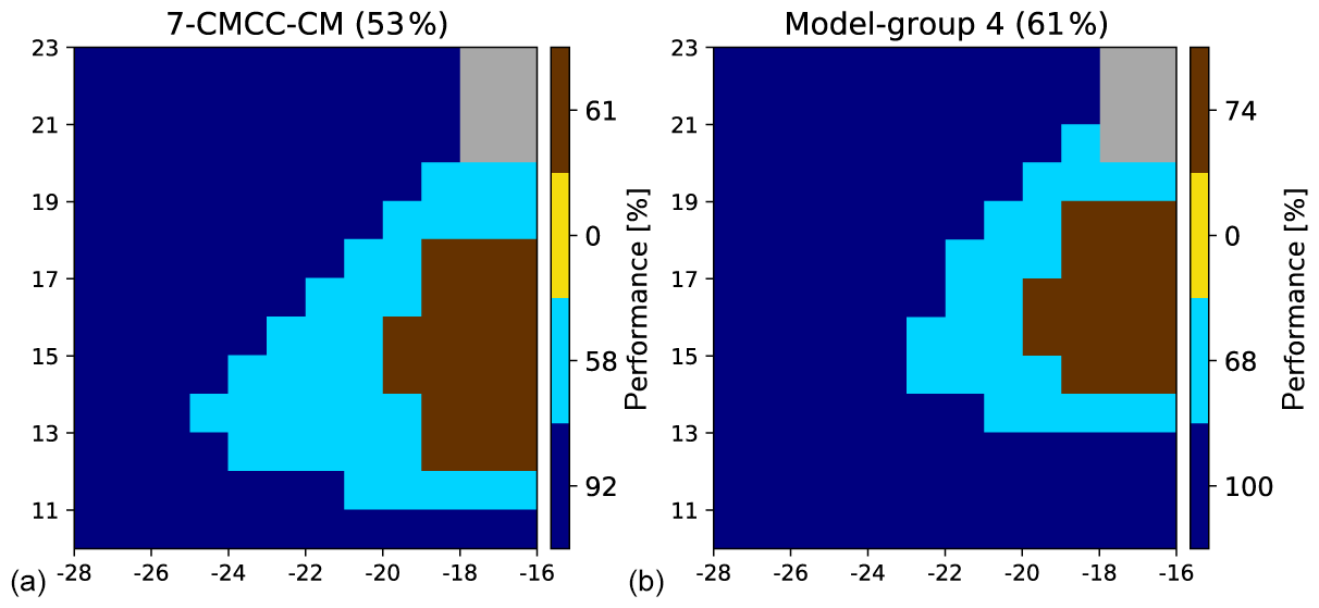
Figure 9Same as Fig. 7 but for the individual model CMCC-CM (model 7) (a) and model group 4 (b).
6.1 Representation of the upwelling in the CMIP5 climate model clusters
In this section, we compare the representation of the Senegalo-Mauritanian upwelling system given by the two best model groups identified above (model group 4 and ZModel group 2). For this evaluation, we use two of the five indices used by Sylla et al. (2019) to evaluate the full database, namely the intensity of the SST seasonal cycle and the offshore Ekman transport at the coast. The former is specific to the seasonal variability of the Senegalo-Mauritanian upwelling system, and it has been used for the classification. The latter is more general and, although it has recently been shown to partly represent the volume of the upwelled waters (Jacox et al., 2018), it is extensively used in the scientific literature to characterize upwelling regions (Cropper et al., 2014; Rykaczewski et al., 2015; Wang et al., 2015). Note also that, following Sylla et al. (2019), evaluation is performed on the period [1985–2005]. This period slightly differs from the classification period, but the SST seasonal cycle is not significantly different (not shown).
Figure 10 compares the amplitude of the SST seasonal cycle as represented in the observations, Model-All, Model-group 4 and ZModel-group 2 identified above. Consistently with Figs. 6 and 8, Model-All dramatically underestimates the upwelling signature in terms of the SST seasonal cycle as compared to the observations. Model-group 4 and ZModel-group 2 yield improved results: the area of an enhanced SST seasonal cycle is larger in both latitude and longitude, with stronger SST amplitude values. This confirms the efficiency of the selection operated above. Nevertheless, ZModel-group 2 yields a realistic SST amplitude pattern along the coast, but it extends too far offshore. Furthermore, in ZModel-group 2, the subtropical area (in green in Fig. 10) extends too far towards the south, in particular in the western part of the basin. The tropical area, characterized by limited amplitude of the seasonal cycle of SST (deep blue in Fig. 10), is shifted to the south as compared to the observations. In other words, the large-scale thermal – and thus probably dynamical – structure of the region is poorly represented in ZModel-group 2. Finally, Model-group 4 is the least biased one.
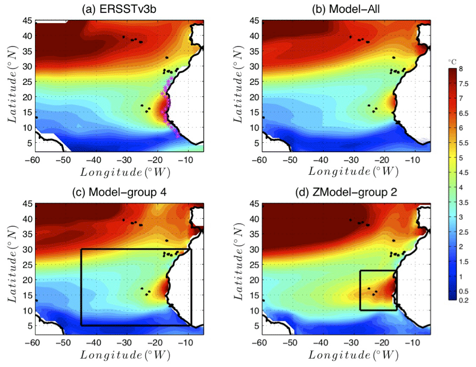
Figure 10Amplitude of the SST seasonal cycle in (a) ERSSTv3b observations (b) Model-All, (c) Model-group 4 (best model group for the extended area, illustrated by the black rectangular box) and (d) ZModel-group 2 (best model group for the reduced area, illustrated by the small black rectangular box). The SST seasonal cycle is computed over the period 1985–2005.
The intensity of the wind stress parallel to the coast, inducing offshore Ekman transport and consequently an Ekman pumping at the coast, is generally considered to be the main driver of the upwelling. We therefore also tested the representation of this driver in the different model groups. The idea is to evaluate the impact of the model selection performed above on the representation of an independent variable by the model groups. Figure 11 shows the latitude–time evolution of the meridional oceanic wind stress, considering that the coast in the studied region is oriented approximately meridionally, so that the offshore Ekman transport is mainly zonal. Note that in Fig. 11, southward winds have positive values, so that they correspond to a westward Ekman transport favorable to upwelling. Panel a shows that the observed meridional wind stress is, all year long, favorable to the upwelling north of 20∘ N. At these latitudes, the meridional wind stress is stronger in summer. Conversely, between 12 and 20∘ N, in the latitude band of the Senegalo-Mauritanian upwelling, the wind blows southward with a very weak intensity in summer, and it even changes direction in the southern part of this latitude band. It is favorable to the upwelling in winter–spring, which explains why the Senegalo-Mauritanian upwelling occurs during this season with a maximum of intensity in March–April (Capet et al., 2017; Farikou et al., 2015). The main bias of Model-All (Fig. 11b) is due to the fact that the wind stress never reverses between 12 and 20∘ N. It weakens in the southern part of the Senegalo-Mauritanian latitude band, i.e., south of the Cape Verde peninsula (15∘ N), but does not become negative. North of the Cape Verde peninsula, it also blows from the north in summer, so that the Senegalo-Mauritanian upwelling lacks seasonality. This bias is corrected in Model-group 4 and ZModel-group 2 (Fig. 11c and d) that are, in this aspect, more realistic than Model-All. Model-group 4 shows a slight extension of the time and latitude range where the oceanic wind stress reverses sign. This constitutes an improvement. The southward wind is nevertheless too strong in winter on the [12–20∘ N] latitude band as well as further south from December to March. These two remaining biases are further reduced in ZModel-group 2. This latter model yields the most realistic seasonal cycle of meridional oceanic wind stress on the latitude band under study. This is consistent with a very localized model selection, as the wind index is itself localized along the coast.
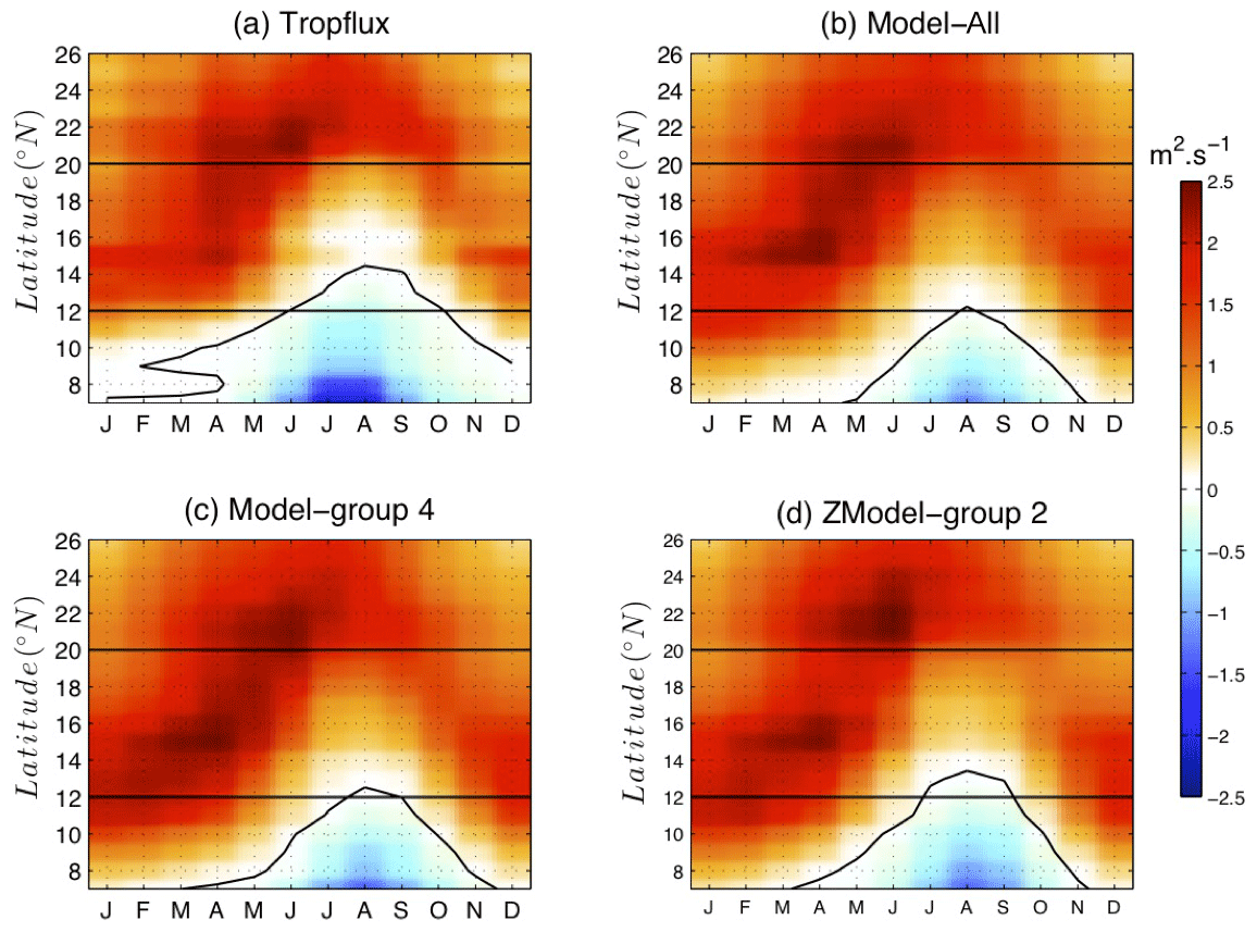
Figure 11Latitude–time plot of depth-integrated Ekman transport computed over the grid point located along the coast (magenta stars in Fig. 9a). The time axis shows climatological months over the period 1985–2005. Positive (negative) values correspond to upwelling (downwelling) conditions. Panel (a) stands for the TropFlux data set (see Praveen Kumar et al., 2011) (b) Model-All, (c) Model-group 4 and (d) ZModel-group 2. In each panel, the black contour shows the contour zero. The horizontal dashed lines are positioned at 12 and 20∘ N and give a rough delimitation of the Senegalo-Mauritanian upwelling region.
To conclude, Model-group 4 and ZModel-group 2 perform in general better than Model-All in reproducing the major, characteristic features of the Senegalo-Mauritanian upwelling. This result confirms the relevance of the multi-model selection we have presented above. Applying the methodology over a relatively large region allows better constraint of the spatial extent and pattern of the SST signature of the upwelling than the reduced area. The latter however yields a better representation of the wind seasonality along the coast.
6.2 Response of the Senegalo-Mauritanian upwelling to global warming
In this section, we examine the response of the upwelling system given by the different multi-model groups we selected to global warming. For this, we compared the two indices analyzed above in present-day and future conditions. The present-day conditions are taken as above as the climatological average of historical simulations over the period [1985–2005]. The future period is taken as the climatological average of the RCP8.5 scenario over the period [2080–2100]. Figure 12 shows the difference of the SST seasonal cycle amplitude between these two periods. The general behavior is that the SST cycle amplitude will reduce in the upwelling region. Sylla et al. (2019) showed that this is primarily due to a warming of the winter temperature, thus suggesting that the upwelling signature at the surface will reduce. On the other hand, this figure shows that the upwelling signature will increase along the Canary Current, which flows along the coast of Morocco, as well as in the subtropical part of our domain. This behavior is observed in the three multi-model ensembles. However, the two selected model groups suggest a weaker decrease in the SST seasonal cycle in the upwelling region than the one given by Model-All. ZModel-group 2 shows an even weaker decrease mainly confined in the southern part of the upwelling region. This result echoes findings of Sylla et al. (2019) based on another indicator of the upwelling imprint on the SST: they showed that the difference between the SST at the coast and offshore is expected to decrease more in the southern part of the Senegalo-Mauritanian upwelling system (SMUS) than in the north. We hypothesize that the study conducted on the reduced area permits separation of the Senegalo-Mauritanian upwelling system into two clusters, a northern one (ZRegion 4) and a southern one (ZRegion-3) (Fig. 8), which enables us to distinguish this specific response.
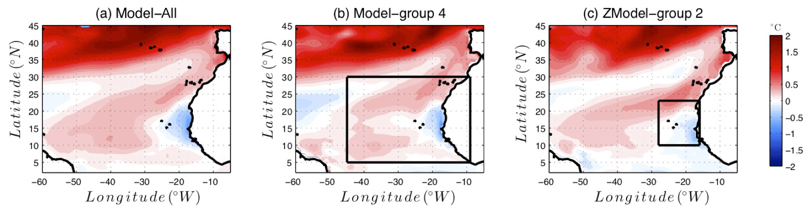
Figure 12Evolution of the amplitude of the SST seasonal cycle at the end of the 21st century. The figure shows the difference between the seasonal cycle amplitude averaged over the period (2080–2100) following the RCP8.5 scenario and the amplitude averaged over the period (1985–2005) in the historical simulations. A positive value (red) means that the seasonal cycle is more marked over the period 2080–2100.
The meridional wind stress also generally weakens under climate change in the [12–20∘ N] latitude band (Fig. 13), suggesting a general reduction of the upwelling intensity. From December to March, this is particularly true in the southernmost region of the Senegalo-Mauritanian band, consistent with the results of Sylla et al. (2019). The wind pattern inferred from the two model groups (Fig. 13b and c) present a higher seasonal variability than those of Model-All (Fig. 13a). The winter reduction of the southward wind stress is slightly more confined to the southern region in ZModel-group 2, especially at the end of the upwelling season (March–April), when the upwelling intensity is the strongest. This may be consistent with the reduced seasonal cycle in the southernmost part of the upwelling identified above.
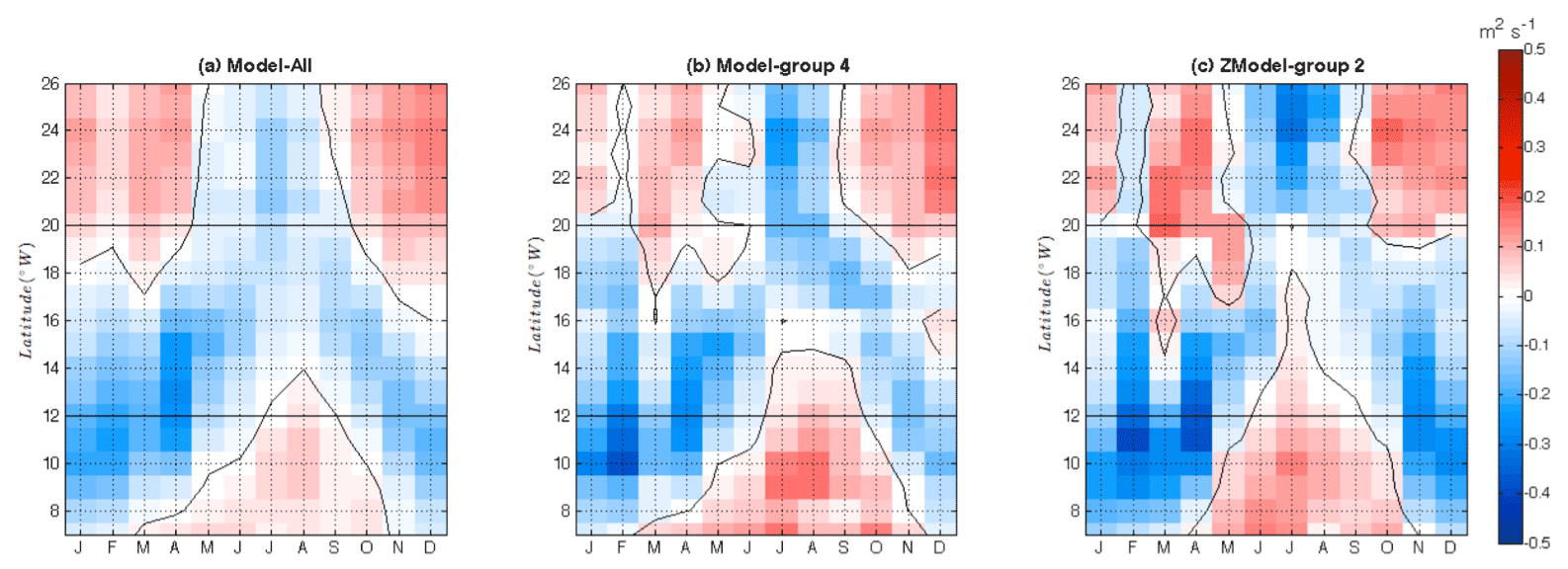
Figure 13 Latitude–time diagram of the seasonal shift of the meridional component of the wind stress with respect to the present day. For each month and at each latitude, we show the meridional wind stress shift with respect to the present day averaged over the period 2080–2100. Positive values (red) mean that the wind stress shift is southward and is thus favorable to upwelling. Panel (a) stands for Model-All, (b) Model-group 4 and (c) ZModel-group 2.
This paper proposed a novel methodology for selecting efficient climate models in a specific area with respect to observations and according to well-defined statistical criteria. The present study has specifically focused on the ability of climate models to reproduce the ocean SST annual cycle observed in specific sub-regions of the studied domain during the period 1975–2005 as reported in the ERSST_v3b data set. These sub-regions were defined by a neural classifier (SOM) as clusters with similar seasonal SST cycle anomalies with respect to some statistical characteristics and were therefore named region clusters. They correspond to ocean areas with well-marked oceanographic specificities.
We then checked the ability of the different climate models to reproduce the region clusters defined on the observation data set with a SOM. The better a climate model fits the clusters computed with the SST observation, the higher the skill of the model. To evaluate this, we defined geographical regions in the different CMIP5 climate models by projecting the SST annual cycle anomalies of each model grid point onto the SOM. Each grid point is associated with a cluster on the SOM and consequently with a region cluster on the geographical map. We built a similarity criterion by counting the number of grid points in a region cluster of a given model matching the same region cluster defined by processing the observation field. We then computed the ratio between that matching number and the number of pixels of the region cluster of the model under study. We estimated the total skill of a model by averaging the seven ratios associated with the seven region clusters. Note that this procedure presents the advantage of giving the same weight to each region cluster whatever its number of grid points and its proximity to the upwelling region. This procedure respects the clustering done by the SOM since the different clusters have an equal weight in the skill computation. In its present definition, the total skill is a number between 0 and 1: the higher the skill, the better the fit. Other measures of the total skill of a model group could nevertheless be defined depending on the objective of the study. One may compare the skill of individual models over a specific region cluster of interest or analyze the pattern of skill in one specific model and its sensitivity to possible various parameterization schemes. The extraction of information embedded in the vector skill whose seven components are the skills associated with the seven sub-regions and the resulting efficient multi-model combination imply the use of advanced statistical tools such as the MCA. Moreover, the vector skill also contains information behavior of models in terms of large offshore ocean circulation as well as in the upwelling region. It could thus be used to diagnose the deficiencies of some climate models with respect to the modeling of physical processes. Another contribution of the MCA is the visualization of the 47 models and the observations on the plane constituted by the first two MCA axes, which represents 70 % of the information embedded in the data. The similarities of the climate models with respect to the observations and the region clusters can be clearly visualized. The “mean” skill associated with each climate model and proposed in this study is easy to use but is far less informative than the vector skill whose seven components are the skills associated with the seven sub-regions.
Such a multi-model ensemble selection allows sampling of a set of models in order to obtain a more realistic climatology over the region of interest. The response of the upwelling to climate change given by the different multi-model ensembles is quite robust in the sense that they give similar qualitative answers. However, a too-selective ensemble of models may lead to noisy patterns. A compromise thus has to be found: a large number of models leads to smoothed biases and unrealistic patterns but also damps the characteristics of the selection. On the other hand, selecting the most realistic models may yield spurious biases in the ensemble mean.
As discussed in the introduction, different criteria have been used for extracting some efficient models from the CMIP5 models used for climatic studies. The most common parameter is the average annual surface mean temperature of the grid points of the region under study. However, Knutti et al. (2006) used the seasonal cycle in surface temperature, represented by the seasonal amplitude calculated as summer June–August (JJA) minus winter December–February (DJF) temperatures. This criterion is more informative than the annual mean temperature since the amplitude of the seasonal variability is an important criterion characterizing the validity of a climate model. In the present work, we used a more informative criterion which is formed from the monthly temperature cycle anomaly represented by a 12-component vector, each component representing the average monthly temperature of the year we consider. This new criterion allows account to be taken of the amplitude and phase of seasonal variability, while the Knutti et al. (2006) criterion only takes into account the amplitude of the seasonal variability. Note however that it implies a good geophysical knowledge of the region under interest, in order to determine the relevant region clusters after the SOM. It is also very specific to the Senegal-Mauritania upwelling region. Furthermore, Sylla et al. (2019) extensively discussed the possible differences among several indices, aiming at characterizing the upwelling and the need to use some of them to have a complete understanding of this coastal phenomenon. This conclusion is probably general to any physical process of the climate system. In the present study, the model selection is based on only one signature of the SMUS. Several possibilities can be envisaged to improve the resolution of this problem, such as merging several indices like SST, temperature at several depths, wind vector or ocean currents. This approach could also allow a selection of models based on the representation of several distinct regional behaviors. In spite of several subjective choices, including the studied domain and the statistical metrics, we argue that this method is a step towards an objective selection of models, based on a quantitative assessment rather than a qualitative analysis of maps of performance.
The methodology is general and can be adapted to any climate or oceanographic phenomenon. Different applications of the multi-model selection strategy proposed in the present study can also be envisaged. Firstly, from a purely modeling point of view, the projection of the models onto the SOM (or ZSOM) and the results of the HAC yield a very enlightening description of a given model behavior in terms of region clusters of the area under study. Such a procedure could advantageously be used by individual modeling groups to identify, analyze and therefore hopefully reduce their model biases in a targeted region. Secondly, from a physical point of view, an identified model group can be used to analyze the targeted region (here the SMUS) in terms of processes, with the advantages of a subset of models which have been selected from quantitative criteria. Such an application has been briefly illustrated by showing how the selected model group represents an important additional characteristic of the SMUS not used for the selection, namely Ekman pumping. A promising reduction of biases of the full multi-model mean ensemble has been identified, opening possibilities for process studies based on this sub-ensemble of the CMIP5 database. A third application of the selection lies in the prediction of the future climate. Here, we have shown that selected multi-model ensembles may provide a more precise description of the future behavior of the SMUS. It may nevertheless be important to note that these conclusions are based on the assumption that the CMIP5 models, which have been selected according to their present-day characteristics, are the most reliable in terms of future projections, which can be questioned and refined (Lutz et al., 2016; Reifen and Toumi, 2009).
As discussed in the introduction, the concept of “model democracy”, suggesting that all models should be equally considered in multi-model ensembles, is now strongly questioned (Knutti et al., 2017). The present study proposes a promising way to improve the quality of multi-model ensembles in terms of model selection. Deep advances in the field of multi-model analysis and selection can be expected from the emerging topic of climate informatics (Monteleoni et al., 2016), as has been shown through the present study. Machine learning can indeed provide efficient tools to make the best out of the extraordinary but imperfect tools that are the climate models and multi-model intercomparison efforts.
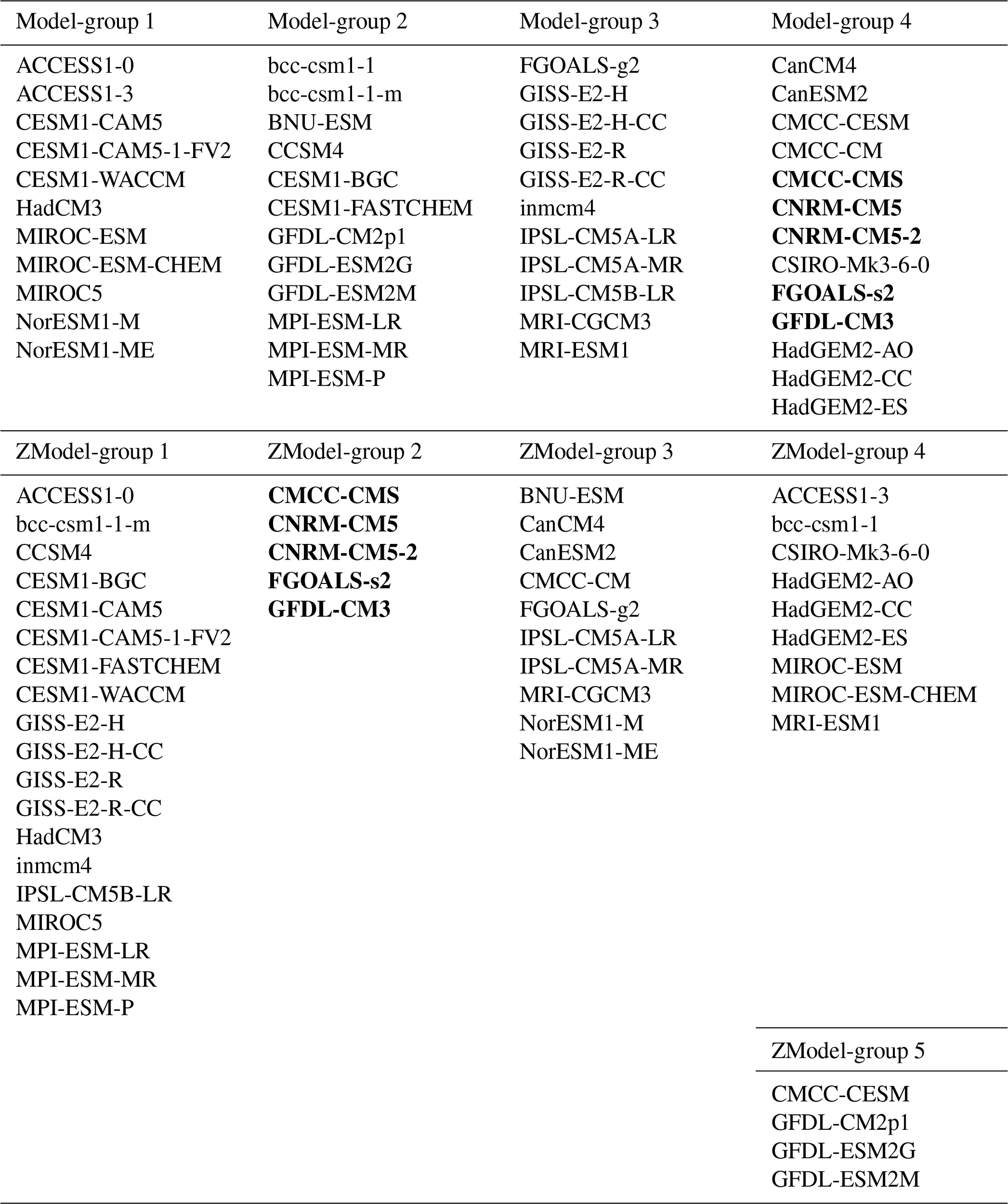
Table A1Composition of the different model groups identified in the main text. In bold, we show the CMIP5 models which belong to Model-group 4 and ZModel-group 2. We note that all the models belonging to Zmodel-group 2 also belong to Model-group 4.
The model output used for this study is freely available on the ESGF database, for example following this url: https://esgf-node.ipsl.upmc.fr/search/cmip5-ipsl/ (Taylor et al., 2012). The SST data were provided by the NOAA/OAR/ESRL PSL, Boulder, Colorado, USA, from their website at https://psl.noaa.gov/ (Smith the al., 2008) and the wind data here: https://podaac.jpl.nasa.gov (Praveen Kumar et al., 2011). The code developed for the core computations of this study can be found under https://doi.org/10.5281/zenodo.3476724 (Mejia and Sorror, 2019). This code allows reproduction of Figs. 2, 3, 6, 7 and 8.
JM initially proposed the idea, ST and MC translated it in terms of methodology and coordinated the method development, CS and CM developed the code and produced the figures, and CS, CM, MC, and ST all contributed to the statistical analysis. AS provided the initial definition of the upwelling index and performed the analysis under climate change that is presented in Sect. 6. JM, MC and ST prepared the manuscript with contributions from all the authors.
NOAA_ERSST_V3b data are provided by the NOAA/OAR/ESRL PSD, Boulder, Colorado, USA, from their website at https://www.esrl.noaa.gov/psd/ (last access: 16 June 2020). The authors are grateful to Matthew Menary for a careful reading of the manuscript.
The research leading to these results has received funding from the NERC/DFID Future Climate for Africa program under the SCUS-2050 project, emanating from the AMMA-2050 project, grant no. NE/M019969/1. The authors are also grateful for support from the Laboratoire Mixte International ECLAIRS2, supported by the French Institut de Recherche pour le Développement. Juliette Mignot was also supported by the H2020-EUCP project under grant agreement 776613. To analyze the CMIP5 data, this study benefited from the IPSL Prodiguer-Ciclad facility which is supported by CNRS, UPMC, Labex L-IPSL which is funded by the ANR (grant no. ANR-10-LABX-0018) and part of the “Investissements d'avenir” program with the reference ANR-11-IDEX-0004-17-EURE-0006 and the European FP7 IS-ENES2 project (grant no. 312979).
This paper was edited by Paul Halloran and reviewed by two anonymous referees.
Borodina, A., Fischer, E. M., and Knutti, R.: Potential to constrain projections of hot temperature extremes, J. Climate, 30, 9949–9964, https://doi.org/10.1175/JCLI-D-16-0848.1, 2017.
Capet, X., Estrade, P., Machu, E., Ndoye, S., Grelet, J., Lazar, A., Marié, L., Dausse, D., Brehmer, P., Capet, X., Estrade, P., Machu, E., Ndoye, S., Grelet, J., Lazar, A., Marié, L., Dausse, D., and Brehmer, P.: On the Dynamics of the Southern Senegal Upwelling Center: Observed Variability from Synoptic to Superinertial Scales, J. Phys. Oceanogr., 47, 155–180, https://doi.org/10.1175/JPO-D-15-0247.1, 2017.
Collins, M., Knutti, R., Dufresne, J.-L., Fichefet, T., Friedlingstein, P., Gao, X., Gutowski, W. J., Johns, T., Krinner, G., Shongwe, M., Tebaldi, C., Weaver, A. J., and Wehner, M.: Long-term Climate Change: Projections, Commitments and Irreversibility, in Climate Change 2013: The Physical Science Basis. Contribution of Working Group I to the Fifth Assessment Report of the Intergovernmental Panel on Climate Change, edited by: Stocker, T. F., Qin, G.-K. D., Plattner, M., Tignor, S. K., Allen, J., Boschung, A., Nauels, Y., Xia, Y., Bex, P. M., and Midgley, V., Cambridge University Press, Cambridge, United Kingdom and New York, NY, USA, 2014.
Cox, P. M., Pearson, D., Booth, B. B., Friedlingstein, P., Huntingford, C., Jones, C. D., and Luke, C. M.: Sensitivity of tropical carbon to climate change constrained by carbon dioxide variability, Nature, 494, 341–344, https://doi.org/10.1038/nature11882, 2013.
Cropper, T. E., Hanna, E., and Bigg, G. R.: Spatial and temporal seasonal trends in coastal upwelling off Northwest Africa, 1981-2012, Deep. Res. Pt. I, 86, 94–111, https://doi.org/10.1016/j.dsr.2014.01.007, 2014.
Deangelis, A. M., Qu, X., Zelinka, M. D., and Hall, A.: An observational radiative constraint on hydrologic cycle intensification, Nature, 528, 249–253, https://doi.org/10.1038/nature15770, 2015.
Demarcq, H. and Faure, V.: Coastal upwelling and associated retention indices derived from satellite SST. Application to Octopus vulgaris recruitment, Oceanol. Acta, 23, 391–408, https://doi.org/10.1016/S0399-1784(00)01113-0, 2000.
Farikou, O., Sawadogo, S., Niang, A., Diouf, D., Brajard, J., Mejia, C., Dandonneau, Y., Gasc, G., Crepon, M., and Thiria, S.: Inferring the seasonal evolution of phytoplankton groups in the Senegalo-Mauritanian upwelling region from satellite ocean-color spectral measurements, J. Geophys. Res.-Oceans., 120, 6581–6601, https://doi.org/10.1002/2015JC010738, 2015.
Fasullo, J. T. and Trenberth, K. E.: A less cloudy future: The role of subtropical subsidence in climate sensitivity, Science, 338, 792–794, https://doi.org/10.1126/science.1227465, 2012.
Faye, S., Lazar, A., Sow, B. A., and Gaye, A. T.: A model study of the seasonality of sea surface temperature and circulation in the Atlantic North-eastern Tropical Upwelling System, Front. Phys., 3, 1–20, https://doi.org/10.3389/fphy.2015.00076, 2015.
Gao, Y., Lu, J. and Leung, L. R.: Uncertainties in projecting future changes in atmospheric rivers and their impacts on heavy precipitation over Europe, J. Climate, 29, 6711–6726, https://doi.org/10.1175/JCLI-D-16-0088.1, 2016.
Gordon, N. D., Jonko, A. K., Forster, P. M., and Shell, K. M.: An observationally based constraint on the water-vapor feedback, J. Geophys. Res.-Atmos., 118, 12435–12443, https://doi.org/10.1002/2013JD020184, 2013.
Hewitson, B. C. and Crane, R. G.: Self-organizing maps: Applications to synoptic climatology, Clim. Res., 22, 13–26, https://doi.org/10.3354/cr022013, 2002.
Huber, M. and Knutti, R.: Anthropogenic and natural warming inferred from changes in Earth's energy balance, Nat. Geosci., 5, 31–36, https://doi.org/10.1038/ngeo1327, 2012.
Jacox, M. G., Edwards, C. A., Hazen, E. L., and Bograd, S. J.: Coastal Upwelling Revisited: Ekman, Bakun, and Improved Upwelling Indices for the U.S. West Coast, J. Geophys. Res.-Oceans., 123, 7332–7350, https://doi.org/10.1029/2018JC014187, 2018.
Jain, A. K. and Dubes, R. C.: Algorithms for clustering data, Prentice Hall, Inc., Englewood Cliffs, 1988.
Jouini, M., Lévy, M., Crépon, M., and Thiria, S.: Reconstruction of satellite chlorophyll images under heavy cloud coverage using a neural classification method, Remote Sens. Environ., 131, 232–246, https://doi.org/10.1016/j.rse.2012.11.025, 2013.
Jouini, M., Béranger, K., Arsouze, T., Beuvier, J., Thiria, S., Crépon, M. and Taupier-Letage, I.: The Sicily Channel surface circulation revisited using a neural clustering analysis of a high-resolution simulation, J. Geophys. Res. Ocean., 121(7), 4545–4567, https://doi.org/10.1002/2015JC011472, 2016.
Knutti, R., Meehl, G. A., Allen, M. R., and Stainforth, D. A.: Constraining climate sensitivity from the seasonal cycle in surface temperature, J. Climate, 19, 4224–4233, https://doi.org/10.1175/JCLI3865.1, 2006.
Knutti, R., Furrer, R., Tebaldi, C., Cermak, J., Meehl, G. A., Knutti, R., Furrer, R., Tebaldi, C., Cermak, J., and Meehl, G. A.: Challenges in Combining Projections from Multiple Climate Models, J. Climate, 23, 2739–2758, https://doi.org/10.1175/2009JCLI3361.1, 2010.
Knutti, R., Sedláček, J., Sanderson, B. M., Lorenz, R., Fischer, E. M., and Eyring, V.: A climate model projection weighting scheme accounting for performance and interdependence, Geophys. Res. Lett., 44, 1909–1918, https://doi.org/10.1002/2016GL072012, 2017.
Kohonen, T.: Essentials of the self-organizing map, Neural Networks, 37, 52–65, https://doi.org/10.1016/j.neunet.2012.09.018, 2013.
Kounta, L., Capet, X., Jouanno, J., Kolodziejczyk, N., Sow, B., and Gaye, A. T.: A model perspective on the dynamics of the shadow zone of the eastern tropical North Atlantic – Part 1: the poleward slope currents along West Africa, Ocean Sci., 14, 971–997, https://doi.org/10.5194/os-14-971-2018, 2018.
Lambert, S. M. and Boer, G. J.: CMIP1 evaluation and intercomparison of coupled climate models, Clim. Dynam., 17, 83–106, https://doi.org/10.1007/pl00013736, 2001.
Liu, Y., Weisberg, R. H., and Mooers, C. N. K.: Performance evaluation of the self-organizing map for feature extraction, J. Geophys. Res.-Oceans., 111, C05018, https://doi.org/10.1029/2005JC003117, 2006.
Loeb, N. G., Wang, H., Cheng, A., Kato, S., Fasullo, J. T., Xu, K.-M., and Allan, R. P.: Observational constraints on atmospheric and oceanic cross-equatorial heat transports: revisiting the precipitation asymmetry problem in climate models, Clim. Dynam., 46, 3239–3257, https://doi.org/10.1007/s00382-015-2766-z, 2015.
Lutz, A. F., ter Maat, H. W., Biemans, H., Shrestha, A. B., Wester, P., and Immerzeel, W. W.: Selecting representative climate models for climate change impact studies: an advanced envelope-based selection approach, Int. J. Climatol., 36, 3988–4005, https://doi.org/10.1002/joc.4608, 2016.
Mejia, C. and Sorror, C.: ClimModEns v1.0, Zenodo, 10.5281/zenodo.3476724, 2019.
Monteleoni, C., Schmidt, G. A., Alexander, F., Niculescu-Mizil, A., Steinhaeuser, K., Tippett, M., Banerjee, A., Benno Blumenthal, M., Ganguly, A. R., Smerdon, J. E., and Tedesco, M.: Climate informatics, in: Computational Intelligent Data Analysis for Sustainable Development, NASA, 81–126, 2016.
Ndoye, S., Capet, X., Estrade, P., Sow, B. A., Dagorne, D., Lazar, A., Gaye, A. T., and Brehmer, P.: SST patterns and dynamics of the southern Senegal-Gambia upwelling center, J. Geophys. Res.-Oceans., 119, 8315–8335, https://doi.org/10.1002/2014JC010242, 2014.
Niang, A., Gross, L., Thiria, S., Badran, F., and Moulin, C.: Automatic neural classification of ocean colour reflectance spectra at the top of the atmosphere with introduction of expert knowledge, Remote Sens. Environ., 86, 257–271, https://doi.org/10.1016/S0034-4257(03)00113-5, 2003.
Niang, A., Badran, F., Moulin, C., Crépon, M., and Thiria, S.: Retrieval of aerosol type and optical thickness over the Mediterranean from SeaWiFS images using an automatic neural classification method, Remote Sens. Environ., 100, 82–94, https://doi.org/10.1016/j.rse.2005.10.005, 2006.
O'Gorman, P. A., Allan, R. P., Byrne, M. P., and Previdi, M.: Energetic Constraints on Precipitation Under Climate Change, Surv. Geophys., 33, 585–608, https://doi.org/10.1007/s10712-011-9159-6, 2012.
Phillips, T. J. and Gleckler, P. J.: Evaluation of continental precipitation in 20th century climate simulations: The utility of multimodel statistics, Water Resour. Res., 42, W03202, https://doi.org/10.1029/2005WR004313, 2006.
Praveen Kumar, B., Vialard, J., Lengaigne, M., Murty, V. S. N., and McPhaden, M. J.: TropFlux: air-sea fluxes for the global tropical oceans – description and evaluation, Clim. Dynam., 38, 1521–1543, https://doi.org/10.1007/s00382-011-1115-0, 2011.
Rayner, N. A.: Global analyses of sea surface temperature, sea ice, and night marine air temperature since the late nineteenth century, J. Geophys. Res., 108, 4407, https://doi.org/10.1029/2002JD002670, 2003.
Reichler, T. and Kim, J.: How well do coupled models simulate today's climate?, B. Am. Meteorol. Soc., 89, 303–311, https://doi.org/10.1175/BAMS-89-3-303, 2008.
Reifen, C. and Toumi, R.: Climate projections: Past performance no guarantee of future skill?, Geophys. Res. Lett., 36, 1–5, https://doi.org/10.1029/2009GL038082, 2009.
Reusch, D. B., Alley, R. B., and Hewitson, B. C.: North Atlantic climate variability from a self-organizing map perspective, J. Geophys. Res.-Atmos., 112, D02104, https://doi.org/10.1029/2006JD007460, 2007.
Richardson, A. J., Risi En, C., and Shillington, F. A.: Using self-organizing maps to identify patterns in satellite imagery, Prog. Oceanogr., 59, 223–239, https://doi.org/10.1016/j.pocean.2003.07.006, 2003.
Rykaczewski, R. R., Dunne, J. P., Sydeman, W. J., García-Reyes, M., Black, B. A., and Bograd, S. J.: Poleward displacement of coastal upwelling-favorable winds in the ocean's eastern boundary currents through the 21st century, Geophys. Res. Lett., 42, 6424–6431, https://doi.org/10.1002/2015GL064694, 2015.
Santer, B. D., Taylor, K. E., Gleckler, P. J., Bonfils, C., Barnett, T. P., Pierce, D. W., Wigley, T. M. L., Mears, C., Wentz, F. J., Bruggemann, W., Gillett, N. P., Klein, S. A., Solomon, S., Stott, P. A., and Wehner, M. F.: Incorporating model quality information in climate change detection and attribution studies, P. Natl. Acad. Sci. USA, 106, 14778–14783, https://doi.org/10.1073/pnas.0901736106, 2009.
Sawadogo, S., Brajard, J., Niang, A., Lathuiliere, C., Crépon, M., and Thiria, S.: Analysis of the Senegalo-Mauritanian upwelling by processing satellite remote sensing observations with topological maps, in: Proceedings of the International Joint Conference on Neural Networks, 2826–2832, 2009.
Sirven, J., Mignot, J., and Crépon, M.: Generation of Rossby waves off the Cape Verde Peninsula: the role of the coastline, Ocean Sci., 15, 1667–1690, https://doi.org/10.5194/os-15-1667-2019, 2019.
Smith, T. M., Reynolds, R. W., Peterson, T. C., and Lawrimore, J.: Improvements to NOAA's historical merged land-ocean surface temperature analysis (1880–2006), J. Climate, 21, 2283–2296, https://doi.org/10.1175/2007JCLI2100.1, 2008.
Son, S. W., Gerber, E. P., Perlwitz, J., Polvani, L. M., Gillett, N. P., Seo, K. H., Eyring, V., Shepherd, T. G., Waugh, D., Akiyoshi, H., Austin, J., Baumgaertner, A., Bekki, S., Braesicke, P., Brühl, C., Butchart, N., Chipperfield, M. P., Cugnet, D., Dameris, M., Dhomse, S., Frith, S., Garny, H., Garcia, R., Hardiman, S. C., Jöckel, P., Lamarque, J. F., Mancini, E., Marchand, M., Michou, M., Nakamura, T., Morgenstern, O., Pitari, G., Plummer, D. A., Pyle, J., Rozanov, E., Scinocca, J. F., Shibata, K., Smale, D., Teyssdre, H., Tian, W., and Yamashita, Y.: Impact of stratospheric ozone on Southern Hemisphere circulation change: A multimodel assessment, J. Geophys. Res.-Atmos., 115, D00M07, https://doi.org/10.1029/2010JD014271, 2010.
Stegehuis, A. I., Vautard, R., Ciais, P., Teuling, A. J., Jung, M., and Yiou, P.: Summer temperatures in Europe and land heat fluxes in observation-based data and regional climate model simulations, Clim. Dynam., 41, 455–477, https://doi.org/10.1007/s00382-012-1559-x, 2013.
Stocker, T. F., Qin, D., Plattner, G.-K., Tignor, M., Allen, S. K., Boschung, J., Nauels, A., Xia, Y., Bex, V., and Midgley, P. M. (Eds.): Climate Change 2013: The Physical Science Basis, Contribution of Working Group I to the Fifth Assessment Report of the Intergovernmental Panel on Climate Change, Cambridge University Press, United Kingdom and New York, NY, USA, 2013.
Sylla, A., Mignot, J., Capet, X., and Gaye, A. T.: Weakening of the Senegalo–Mauritanian upwelling system under climate change, Clim. Dynam., 53, 4447–4473, https://doi.org/10.1007/s00382-019-04797-y, 2019.
Tan, I., Storelvmo, T., and Zelinka, M. D.: Observational constraints on mixed-phase clouds imply higher climate sensitivity, Science, 352, 224–227, https://doi.org/10.1126/science.aad5300, 2016.
Taylor, K. E., Stouffer, R. J., Meehl, G. A., Taylor, K. E., Stouffer, R. J., and Meehl, G. A.: An Overview of CMIP5 and the Experiment Design, B. Am. Meteorol. Soc., 93, 485–498, https://doi.org/10.1175/BAMS-D-11-00094.1, 2012.
Tebaldi, C. and Knutti, R.: The use of the multi-model ensemble in probabilistic climate projections, Philos. T. R. Soc. A, 365, 2053–2075, https://doi.org/10.1098/rsta.2007.2076, 2007.
Wang, D., Gouhier, T. C., Menge, B. A., and Ganguly, A. R.: Intensification and spatial homogenization of coastal upwelling under climate change, Nature, 518, 390–394, https://doi.org/10.1038/nature14235, 2015.
Wenzel, S., Cox, P. M., Eyring, V., and Friedlingstein, P.: Emergent constraints on climate-carbon cycle feedbacks in the CMIP5 Earth system models, J. Geophys. Res.-Biogeo., 119, 794–807, https://doi.org/10.1002/2013JG002591, 2014.
Wenzel, S., Eyring, V., Gerber, E. P., and Karpechko, A. Y.: Constraining future summer austral jet stream positions in the CMIP5 ensemble by process-oriented multiple diagnostic regression, J. Climate, 29, 673–687, https://doi.org/10.1175/JCLI-D-15-0412.1, 2016.
- Abstract
- Introduction
- Climate models and region of interest
- Comparing observations and models: a methodological approach
- Qualitative analysis of the climate models
- Analysis of the climate models over a zoomed upwelling region
- Impact of climate change on the Senegalo-Mauritanian upwelling
- Discussion and conclusion
- Appendix A
- Code and data availability
- Author contributions
- Acknowledgements
- Financial support
- Review statement
- References