the Creative Commons Attribution 4.0 License.
the Creative Commons Attribution 4.0 License.
 | 26 May 2020
Ocean biogeochemistry in the Norwegian Earth System Model version 2 (NorESM2)
Jerry F. Tjiputra
Jörg Schwinger
Mats Bentsen
Anne L. Morée
Shuang Gao
Ingo Bethke
Christoph Heinze
Nadine Goris
Alok Gupta
Yan-Chun He
Dirk Olivié
Øyvind Seland
Michael Schulz
The ocean carbon cycle is a key player in the climate system through its role in regulating the atmospheric carbon dioxide concentration and other processes that alter the Earth's radiative balance. In the second version of the Norwegian Earth System Model (NorESM2), the oceanic carbon cycle component has gone through numerous updates that include, amongst others, improved process representations, increased interactions with the atmosphere, and additional new tracers. Oceanic dimethyl sulfide (DMS) is now prognostically simulated and its fluxes are directly coupled with the atmospheric component, leading to a direct feedback to the climate. Atmospheric nitrogen deposition and additional riverine inputs of other biogeochemical tracers have recently been included in the model. The implementation of new tracers such as “preformed” and “natural” tracers enables a separation of physical from biogeochemical drivers as well as of internal from external forcings and hence a better diagnostic of the simulated biogeochemical variability. Carbon isotope tracers have been implemented and will be relevant for studying long-term past climate changes. Here, we describe these new model implementations and present an evaluation of the model's performance in simulating the observed climatological states of water-column biogeochemistry and in simulating transient evolution over the historical period. Compared to its predecessor NorESM1, the new model's performance has improved considerably in many aspects. In the interior, the observed spatial patterns of nutrients, oxygen, and carbon chemistry are better reproduced, reducing the overall model biases. A new set of ecosystem parameters and improved mixed layer dynamics improve the representation of upper-ocean processes (biological production and air–sea CO2 fluxes) at seasonal timescale. Transient warming and air–sea CO2 fluxes over the historical period are also in good agreement with observation-based estimates. NorESM2 participates in the Coupled Model Intercomparison Project phase 6 (CMIP6) through DECK (Diagnostic, Evaluation and Characterization of Klima) and several endorsed MIP simulations.
- Article
(37255 KB) - Full-text XML
-
Supplement
(3042 KB) - BibTeX
- EndNote


Up to the early 1990s, climate models consisted only of physical atmospheric general circulation models (AGCMs) with prescribed ocean surface state variables or simplified ocean modules (swamp ocean, slab ocean). As the ocean is a huge reservoir and an absorber of heat and the greenhouse gas CO2 (carbon dioxide), an expansion of climate models to include ocean components and a representation of the carbon cycle became a necessity. Coupled atmosphere–ocean–land models (now referred to as Earth system models – ESMs) were eventually developed to account for further reservoirs and feedbacks, including biogeochemical cycles (Bretherton, 1985; Cubasch et al., 2013; Heinze et al., 2019). The inclusion of the ocean carbon cycle is a first-order requirement because on timescales beyond a few decades, the ocean becomes the sole major sink for atmospheric excess CO2 from anthropogenic emissions (Sarmiento and Gruber, 2006). ESM simulations can therefore be used to estimate historical carbon budgets and future partitioning of carbon fluxes into Earth system reservoirs under specified scenarios.
Today, modern ESMs are state-of-the-art tools utilized to study the complex interactions and feedbacks between various components in the Earth system in a comprehensive way (Flato et al., 2013). They are applied regularly to simulate climate evolutions across timescales and to study transient climate change, its drivers, and its impact on the environment (e.g. Bopp et al., 2013; Gehlen et al., 2014). By prescribing plausible scenarios of future emissions and land use, these models provide projections for possible future climate states. ESMs are typically upgraded every few years with new and improved process representations as well as adaptations to technical advancements (e.g. new hardware systems, higher resolution, etc.).
The ocean and its biogeochemistry play a crucial role in controlling the rate of anthropogenic climate change through a substantial negative feedback (Friedlingstein et al., 2006; Arora et al., 2013). However, the absorption rates of heat and carbon by the ocean are non-linear in space and time due to the complex interactions with the internal climate variability (e.g. Tjiputra et al., 2012; Schwinger et al., 2014). Once past the air–sea interface, the dissolved carbon dioxide reacts with seawater and is chemically transformed into different carbonate species. The ocean circulation and biological processes sequester parts of these into the deep ocean, where they stay isolated from the atmosphere for decades to millennia (Sarmiento and Gruber, 2006). In addition to carbon dioxide, the ocean biogeochemistry also influences the Earth's climate through other seawater chemical constituents, such as dimethyl sulfide emissions. This could result in a number of feedback mechanisms within the Earth system that can either amplify or dampen the rate of climate change (Rhein et al., 2013). ESM projections are therefore critical for narrowing uncertainties in the future global carbon budget and consequently its climate feedback.
ESMs have been increasingly used to estimate the evolution of marine ecosystem stressors, such as ocean acidification and deoxygenation, under anthropogenic climate change (e.g. Gehlen et al., 2014; Tjiputra et al., 2018). ESM applications to support climate policy-making, such as quantifying future compatible anthropogenic carbon emissions under a set of predefined scenarios and addressing emerging questions associated with the United Nations sustainable development goals, have become more regular. With its growing relevance, a more realistic representation of the observed contemporary ocean biogeochemistry in Earth system models is urgently necessary to increase the fidelity of future projections.
In this paper, we present improvements in the ocean biogeochemical component of the Norwegian Earth System Model (NorESM). This component is based on the Hamburg Oceanic Carbon Cycle model (HAMOCC5.1), which was originally developed by Maier-Reimer (1993) and has gone through several development iterations (e.g. Six and Maier-Reimer, 1996; Maier-Reimer et al., 2005). At the Bjerknes Centre for Climate Research in Norway, the model has been branched off, further developed (Assmann et al., 2010; Tjiputra et al., 2010, 2013; Schwinger et al., 2016), and coupled to the Bergen Layered (isopycnic coordinate) Ocean Model (BLOM-iHAMOCC). Within the CMIP5 experiments, we identified several shortcomings in the previous model version of NorESM (NorESM1-ME, hereafter referred to as NorESM1). Here, we discuss several developments relative to the NorESM1 version (described in Tjiputra et al., 2013) in the current model version (NorESM2, Seland et al., 2020a), which contributes to CMIP6.
NorESM1 does not include interactively coupled DMS emissions from the ocean, which is the largest natural source of atmospheric sulfur and contributes to aerosol and cloud formation. Instead, the atmospheric chemistry module of NorESM1 prescribed mean fixed climatology oceanic fluxes of DMS, and there is no feedback associated with climate-induced change in marine biological production. However, a model study has suggested that the inclusion of interactive DMS in future climate projections could potentially result in spatially varying changes in the warming rate and a non-negligible feedback on the climate system (Schwinger et al., 2017). This has prompted us to include a fully interactive DMS cycle (production, emissions, and radiative impact) into NorESM2.
In the past years, the concept of emergent constraints was employed to identify key biogeochemical processes that lead to uncertainties in ESMs projections (e.g. Wenzel et al., 2014; Kwiatkowski et al., 2017). For instance, biases in the seasonal cycles of biological production and surface ocean pCO2 have been identified as factors contributing to the uncertainty in projected carbon sinks and storage in the ESMs participating in CMIP5 (Kessler and Tjiputra, 2016; Goris et al., 2018). These studies motivate further improvement in the representation of biological processes, particularly focusing on high-latitude regions such as the Southern Ocean. The biological improvements in NorESM2 were mainly achieved through tuning of the poorly constrained parameters in the ecosystem module.
In NorESM1, as well as other ESMs participating in CMIP5, there is a large uncertainty in the simulated interior oxygen concentration when compared to observations. This is partly attributed to the short model spin-up and bias in the interior remineralization processes (Cabré et al., 2015; Séférian et al., 2016). To alleviate this, we have tested several parameterizations of particulate organic carbon (POC) sinking schemes in our model (Schwinger et al., 2016). Currently, there are three different sinking schemes that can be selected in NorESM2. Based on our earlier assessments, we have used the scheme with a sinking velocity that increases linearly with depth as the default parameterization in NorESM2.
Increasing atmospheric CO2 and associated climate change will alter both the natural and anthropogenic components of ocean inorganic carbon chemistry. Disentangling the future dynamical responses of these components separately is therefore necessary to identify which processes (e.g. biological and physical, among others) regulate the simulated changes in ocean carbon storage today and in the future. In NorESM1, only a single dissolved inorganic carbon (i.e. total DIC) tracer was implemented, and there is no suitably accurate method to separate between the driving mechanisms of its changes. In NorESM2, we have introduced a new “natural” DIC tracer, which simulates changes in the natural component of DIC (i.e. it only interacts with a fixed pre-industrial CO2 concentration during the air–sea gas exchange). Other key diagnostic tracers such as preformed phosphate, oxygen, and alkalinity have also been implemented, all of which allow us to better elucidate mechanisms driving the simulated ocean carbon chemistry changes (Bernardello et al., 2014). These tracers can also be used to infer interior ocean circulation-induced changes in biogeochemical tracers.
Nutrients are important constraints of ocean primary productivity and hence atmospheric carbon sinks. In NorESM1, the nutrient cycle was assumed to be an approximately closed system with a long-term loss due to sedimentation. The only external source is through atmospheric nitrogen fixation and aerial dust deposition, which is converted into dissolved iron. Implementation of the riverine input of nutrients in HAMOCC5.1 was initiated by Bernard et al. (2011), and a study by Gao et al. (2020) indicates that riverine nutrient inputs could improve the regional representation of marine biogeochemistry, with consequences for future projections; i.e. they increase coastal carbon sinks and alleviate nutrient limitations due to warming-induced stratification. In NorESM2, we have accounted for riverine inputs of nutrients and other biogeochemical constituents. Other processes representing external nitrogen sources such as atmospheric nitrogen deposition and nitrogen fixation have also been implemented and updated, respectively.
Since ESMs are used to project future climate change, questions have arisen as to whether or not these models are able to simulate past climate change. To this end, NorESM1 has been applied to study the sensitivity of climate states to different boundary conditions in the past, going back from the last glacial to as far back as the mid-Pliocene (Zhang et al., 2012; Guo et al., 2019). The model was also used to study the sensitivity of the ocean carbon cycle to different background climates, which could provide insight into the ocean's role in regulating past atmospheric CO2 variability (Kessler et al., 2018; Luo et al., 2018). There has also been a growing interest in determining if such complex models are able to reproduce climate states directly inferred from proxy records. These paleo-proxies, e.g. carbon isotopes (δ13C and δ14C), typically measured from foraminiferal samples collected from seafloor sediment, are natural archives that store water mass properties and are used to infer large-scale ocean circulation patterns as well as ventilation timescales during past climate changes (Peterson et al., 2014). In NorESM2, we have now implemented 13C and 14C tracers, which will be used as an additional ocean circulation and biogeochemistry constraint when simulating past climate variability.
Beyond the above-mentioned biogeochemical processes, other improvements in tracer initialization, iron chemistry, air–sea gas exchange parameterization, code readability, and documentations of the codes have been made. Moreover, there have been several updates within the physical ocean component of NorESM2, and a selection of these updates is discussed in this paper as they have direct impacts on the ocean biogeochemistry. In addition to describing the model improvements, we also evaluate the performance of the ocean biogeochemical component of NorESM2. Whenever possible, we compare and describe the performance of the NorESM2 model with the first-generation model, NorESM1.
The paper is organized as follows: advancements in the physics and more detailed descriptions of all improvements in biogeochemical processes are described in Sect. 2. Implementations of new tracers are presented in Sect. 3. The different model simulations performed and used in the paper are described in Sect. 4. In Sect. 5, we present results from our coupled ESM simulations and the ocean-only (pre-industrial) simulation to illustrate the performance of the simulated carbon isotope tracers. A summary and discussion are presented in Sect. 6.
2.1 General configuration changes
In NorESM2, the ocean–ice model adopts a tripolar grid instead of the bipolar grid of NorESM1. The tripolar grid was chosen because it is more isotropic at northern high latitudes and is therefore more efficient with respect to time integration (longer time step) (Guo et al., 2019). Compared to NorESM1, NorESM2 has enabled a higher-frequency ocean coupling to resolve the diurnal cycle in the flux and state exchange between the ocean and atmosphere (i.e. hourly instead of daily atmosphere–ocean coupling). We also applied a full leapfrog time stepping in both the physical and ocean biogeochemical models to improve the conservation of biogeochemical tracers (Schwinger et al., 2016).
There are several configuration options for NorESM2. For CMIP6, two configurations will mostly be used, differing only in the horizontal resolution of the atmospheric and land models with otherwise identical model components. They are named NorESM2-LM and NorESM2-MM and have an atmosphere–land resolution of approximately 2∘ and 1∘, respectively. In addition, both versions have a different parameter tuning in the atmospheric component, necessary to achieve a top-of-atmosphere radiative balance under pre-industrial conditions. Both NorESM2-LM and NorESM2-MM share the same ocean physical ocean model (BLOM) and the same biogeochemical component (iHAMOCC) with a horizontal resolution of approximately 1∘. The ocean model adopts 53 isopycnal layers with two non-isopycnic surface layers, which represent (1) the top 10 m of depth and (2) the rest of the surface mixed layer. A more detailed description of the ocean physical component is provided in Bentsen et al. (2020). The ocean biogeochemistry performs similarly in both model versions. Unless explicitly specified, our analysis refers to the results from NorESM2-MM (hereafter referred to as NorESM2).
2.2 Physical parameterizations
The simulated Atlantic Meridional Overturning Circulation (AMOC) strength in NorESM1 is on the strong side (30.8 Sv at 26.5∘ N; 1 Sv =106 m3 s−1) compared to observation-based estimates and other CMIP5 models (Bentsen et al., 2013). The vigorous AMOC leads to an Atlantic Ocean that is too warm and saline at depth. Lack of upper-ocean stratification at high latitudes is thought to contribute to this AMOC bias. Reformulating the eddy-induced transport (Gent and McWilliams, 1990) in order to make it more efficient in the upper-ocean non-isopycnic regime of the model and adjustments to the parameterized re-stratification by mesoscale eddies (Fox-Kemper et al., 2008) lead to improved high-latitude stratification and a more realistic mixed layer depth (MLD), particularly at high latitudes.
NorESM1 has a cold bias in the depth range 200–1000 m between 50∘ S and 50∘ N (Bentsen et al., 2013) that could be related to insufficient upper-ocean vertical mixing. Further, the new hourly atmosphere–ocean coupling and associated tuning of MLD parameterizations lead to a cold bias in the Pacific equatorial thermocline that also indicates too little vertical mixing.
To improve this, two different approaches have been used. First, we allow surface turbulent kinetic energy (TKE) originating from wind stirring to penetrate below the mixed layer and be added to the TKE reservoir of the k-ϵ turbulence model handling the shear instability mixing of the isopycnic interior. Secondly, with hourly atmosphere–ocean coupling, high-frequency winds are available to parameterize wind work on near-inertial motions. Inspired by the approach of Jochum et al. (2013), a fraction of this energy source is added to the mixed layer TKE reservoir, modifying the MLD estimation, while a fraction of the remaining energy is used to drive upper-ocean mixing through assumed excitation and breaking of internal waves. Combining these approaches, we were able to reduce the above-mentioned upper-ocean biases significantly. The mid-depth warm bias seen in NorESM1 is also reduced. More details on the physical improvements are described in Bentsen et al. (2020). As a result of these improvements, NorESM2 simulates a more reasonable AMOC strength of approximately 21 Sv, which is within the range of the observational estimates of 17.9±3.3 Sv (Srokosz et al., 2012).
2.3 Dimethyl sulfide
NorESM2 prognostically simulates the DMS concentration according to the formulation of Kloster et al. (2006), as follows:
where the first term on the right-hand side denotes the physical transport, the second term denotes DMS production, and the third, fourth, and fifth terms denote sinks due to bacterial activity, photolysis, and flux to the atmosphere. The production term is computed as a function of temperature, pH, and simulated detritus export production (opal and CaCO3, implicitly computed as a function of silicate concentration):
The last term in Eq. (2) describes a pH dependence of DMS production following Six et al. (2013), which is parameterized based on the deviation of actual pH from the climatological monthly mean surface pH (pHpi) calculated from the pre-industrial control. Due to uncertainties in the pH control on DMS production, we have omitted the pH dependency term by setting α to zero in the presented simulations. Parameters γo and γc represent scaling factors for sulfur (S:Si and S:C) and are set to 0.025 and 0.125, respectively, such that DMS production is more sensitive to CaCO3 production in the model. This assumption is due to the fact that haptophyte-class phytoplankton generally has a higher dimethylsulfoniopropionate-to-cell-carbon ratio than diatoms (Keller et al., 1989). Since the opal and CaCO3 portions of export production are implicitly computed as a function of silicate concentration, e.g. opal (CaCO3) production is high (low) when surface silicate is abundant and vice versa, the DMS production is also sensitive to the long-term trend in the silicate concentration.
The DMS sink due to bacteria consumption is estimated as a function of temperature (∘C), DMS concentration, consumption rate (γbac=0.0864 d−1 ∘C−1), and a half-saturation constant (kcb=10 nmol L−1), as follows:
The DMS photolysis term is defined as a function of photolysis rate (γuv=0.0011 m2 (W d)−1), incoming shortwave radiation attenuated by water and phytoplankton, Iz, and DMS concentration:
Lastly, in NorESM2, the atmospheric model receives the DMS emissions (Sgas) that are prognostically computed by the ocean biogeochemistry model (see Sect. 2.8).
2.4 Riverine input
The influx of carbon and nutrients from over 6000 rivers to the coastal oceans has been implemented based on previous work of Bernard et al. (2011) with modifications. Bernard et al. (2011) have implemented the riverine fluxes based on levels in the year 1995 provided by an early version of the Global-NEWS model (Seitzinger et al., 2005). In addition to the riverine DIC, dissolved organic carbon (DOC), inorganic nitrogen and phosphorus, particulate organic carbon (POC), particulate nitrogen and phosphorus, and dissolved silicate, we have also included riverine alkalinity (ALK) and iron (Fe). Except for DIC, ALK, and Fe, all data are provided by the more recent Global-NEWS2 model (Mayorga et al., 2010), which is a hybrid of empirical, statistical, and mechanistic model components that simulate steady-state annual riverine fluxes of carbon and nutrients. The DIC and ALK fluxes are taken from the work by Hartmann (2009). The riverine Fe flux is calculated as a proportion of global gross dissolved Fe input of 1.45 Tg yr−1 (Chester, 1990), weighted by the water runoff of each river. Only 1 % of the riverine dissolved Fe is added to the oceanic dissolved Fe, since approximately 80 % to 99 % of the fluvial gross dissolved Fe is removed during estuarine mixing (e.g. Sholkovitz et al., 1981; Shiller and Boyle, 1991; Bruland and Lohan, 2014). Instead of releasing the riverine fluxes to the nearest ocean grid cell (Bernard et al., 2011), we have interpolated all fluxes at river mouths in the same way as the freshwater runoff (distributed as a function of river mouth distance with an e-folding length scale of 1000 km and cutoff of 300 km) to the ocean grid. The fluxes are specified to be constant over time at contemporary levels (the year 2000). In our model, the organic form of dissolved carbon (DOC) is connected to nutrients through the Redfield ratio (), and therefore other forms of dissolved organic matter (e.g. DON and DOP) are not explicitly simulated. Since Global-NEWS provides estimates of dissolved organic matter in carbon, nitrogen, and phosphate forms (DOCriv, DONriv, and DOPriv, respectively) separately, only the minimum of the three riverine dissolved organic constituents is added to the DOC term in the model (i.e. DOC = DOC + min(DOCriv, ). Any excess or remaining organic matter of the three constituents is then added to the corresponding inorganic pools (DIC, NO3, or PO4). The same concept also applies to riverine inputs of particulate organic carbon (POC) (see also Bernard et al., 2011).
2.5 Atmospheric nitrogen deposition
We apply anthropogenic nitrogen deposition fluxes that potentially affect the simulated ocean carbon uptake (through an increase in the available nitrate for biological production) to the ocean biogeochemical model. The monthly input fields, spanning the years 1850–2014, are simulated by chemistry transport models and provided by CMIP6 (Jones et al., 2016). Conservative remapping is used to interpolate the input data from a regular latitude–longitude grid to the tripolar ocean model grid of NorESM2. Four species of wet or dry and oxidized or reduced nitrogen deposition rates are included in the input fields. All of them are added to the nitrate pool in the topmost ocean layer.
2.6 Particle export
In NorESM1, the export of particulate organic matter is parameterized with a constant sinking speed and a constant remineralization rate at depth when sufficient oxygen is available. This simplistic formulation has been shown to have difficulty in accurately representing the observed particle fluxes at depths (Kriest and Oschlies, 2008) and leads to biases in the interior distributions of biogeochemical tracers (e.g. as seen from remineralized phosphate concentrations). In NorESM2, we have developed two additional particle flux parameterizations that can be selected. They are referred to as the WLIN and AGG schemes. The WLIN scheme is similar to the standard scheme but the sinking speed is a linear function of depth: , wmax). Here, we use m d−1, m d−1, and m d−1 m−1. When wmin and wmax are set to zero and infinity, respectively, this scheme is equivalent to the widely used Martin curve formulation (Martin et al., 1987).
The AGG scheme implements a prognostic sinking speed calculated according to a size distribution of sinking particles. The total concentration of particulate matter, formulated as a function of phytoplankton and detritus, forms sinking aggregates with an explicitly computed size distribution that follows a power-law formula (Kriest and Evans, 1999; Kriest, 2002):
Here, d represents the particle diameter, and A and β represent parameters of the size distribution. The minimum particle diameter l is set to 0.002 cm. The sinking speed of aggregates is computed according to the diameter of each aggregate. More details of the implementation of the AGG formulation are described in Schwinger et al. (2016). Based on the performance of the different schemes, we have set WLIN to be the default scheme and it is used in all experiments presented here. More details on the differences in the simulated interior biogeochemistry using the different particle export schemes are available in Schwinger et al. (2016).
2.7 Nitrogen fixation
Nitrogen fixation by cyanobacteria is computed implicitly and directly converted into nitrate concentration. In NorESM1, nitrogen fixation is implemented such that it can occur anytime and anywhere in the surface ocean as long as the nitrate concentration is lower than phosphate (multiplied by the stoichiometric nitrate-to-phosphate ratio RN:P following Maier-Reimer et al., 2005). However, Breitbarth et al. (2007) provided some evidence that the large-scale distribution of Trichodesmium, a type of cyanobacteria, is well constrained by seawater temperature between 20 and 30 ∘C. Based on this, a temperature-dependent function f(T) according to Kriest and Oschlies (2015) has been added to the nitrogen fixation formulation in NorESM2. The rate of change of nitrate owing to nitrogen fixation is formulated as follows:
with
where μ is the maximum N2 fixation rate (0.005 d−1). In addition, for each mole of N fixed to nitrate, 1.25 mol of dissolved oxygen and 1 mol of alkalinity are consumed and lost in the surface layer. The corrected formula essentially limits the occurrence of N fixation to warm low latitudes.
2.8 Air–sea gas exchange
In NorESM2, the air–sea gas exchange of CO2, O2, N2, N2O, DMS, CFC-11, CFC-12, and SF6 is computed prognostically according to the updated formulation of Wanninkhof (2014). Here, the air–sea flux F of gas X is computed as a function of surface wind speed U, Schmidt number Sc, gas solubility Ko, and the partial pressure difference of gas X based on a bulk formulation:
The net fluxes are computed for the top layer of the ocean model (i.e. 10 m of depth). The updated formulation includes a refitted temperature-dependent Schmidt number that can be applied for a temperature range of −2 to 40 ∘C. The solubility of all gases is computed as a function of surface temperature and salinity following Weiss (1970) for O2 and N2, Weiss and Price (1980) for CO2 and N2O, Warner and Weiss (1985) for CFC-11 and CFC-12, and Bullister et al. (2002) for SF6. The flux of DMS is only unidirectional (outgassing; pDMSair=0).
In the historical simulation, we use the annual atmospheric concentrations of CFC-11, CFC-12, and SF6 divided into northern and southern hemispheric values according to Bullister (2014). For the atmospheric CO2 concentration, monthly global mean values from the CMIP6 dataset are used. In the pre-industrial simulation, a constant CO2 concentration of 284.32 ppm is used.
2.9 Dissolved iron parameterization
Adjustments in the iron parameterization have been made to ensure that NorESM2 simulates the observed iron-limited primary production in the Southern Ocean, equatorial Pacific, and North Pacific. In the model, the consumption and release of dissolved iron associated with biological activities are determined using a fixed stoichiometry ratio ( mol Fe mol P−1, previously mol Fe mol P−1). In the surface layer, a constant fraction ( kmol Fe kg−1 d−1, previously kmol Fe kg−1 d−1) of aerial dust deposition (Mahowald et al., 2005) is instantaneously converted into bioavailable iron. The updated global input of bioavailable iron from the atmosphere is 2.8 Gmol Fe yr−1, which is within the range of values used by other models (Tagliabue et al., 2016). Finally, throughout the water column, the complexation of iron by organic substances (ligands) is assumed:
where the strength of this complexation λFe is set to 0.05∕365 (previously 0.005∕365) d−1 and the threshold Feo has been reduced from 0.6 to 0.5 nmol Fe m−3. The latter is motivated by the fact that the observed iron concentration in the deep Southern Ocean is lower than 0.6 nmol Fe m−3 (Boyd and Ellwood, 2010). The higher complexation rate leads to a faster relaxation toward this value.
2.10 Ecosystem parameterization updates
The underlying marine ecosystem parameterization in NorESM2 remains the same as in NorESM1, but many of the parameters have been adjusted to reduce biases that are present in NorESM1. The main deficiencies of the spatial annual mean primary productivity pattern in NorESM1 are primary production (PP) that is too strong in the Southern Ocean, the eastern tropical Pacific, and to a lesser degree the North Atlantic, contrasted by very low PP in the subtropical gyres (most pronounced in the Pacific). The high productivity in the high latitudes is accompanied by an exaggerated annual cycle of PP, showing a spring bloom that is too strong and a decline of PP that is too fast afterwards. Tuning of the ecosystem parameterization during the development of NorESM2 was focused on improving these regional shortcomings. The changes in ecosystem parameters listed in Table 1 mainly serve two purposes: (i) to increase top-down limitation by zooplankton grazing during phytoplankton peak bloom (but not before and after) and (ii) to increase the fraction of nutrients that is routed through dissolved organic matter (DOM).
Table 1Parameter values of the ecosystem parameterizations that have been changed between NorESM1, NorESM-OC1.2, and NorESM2. NorESM-OC1.2 was an intermediate model version (Schwinger et al., 2016) and is included here for completeness and traceability. The naming of parameters follows Ilyina et al. (2013).
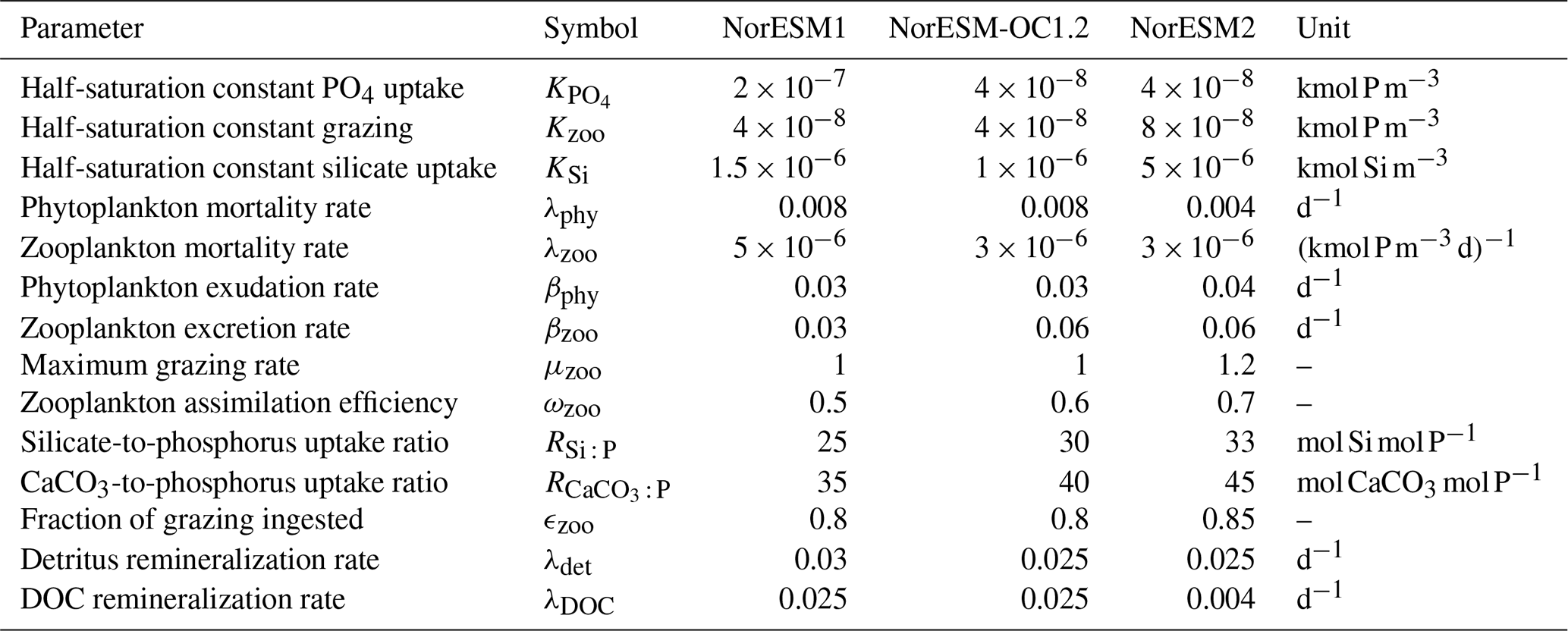
The first point is achieved through a reduction in zooplankton mortality and increases in the maximum grazing rate, assimilation efficiency, and half-saturation constant for zooplankton grazing. The latter point is mainly achieved by reducing the production of detritus by zooplankton (fecal pellets, 1-ϵzoo of grazing) and increasing exudation and excretion rates. This allows, in combination with a decrease in the DOM remineralization constant, more nutrients to be laterally transported out of regions where nutrient trapping occurs, i.e. the tropical Pacific.
Additionally, CaCO3-to-phosphate and silicate-to-phosphate ratios were tuned to remove the high alkalinity bias of NorESM1 (see Schwinger et al., 2016, for details). Note that some adjustments of the parameters given in Table 1 were also necessary because of the new sinking scheme (increasing sinking speed with depth; see Sect. 2.6) and the different physical circulation fields between NorESM1 and NorESM2. An updated schematic diagram of the marine ecosystem module in NorESM2 is presented in Fig. 1.
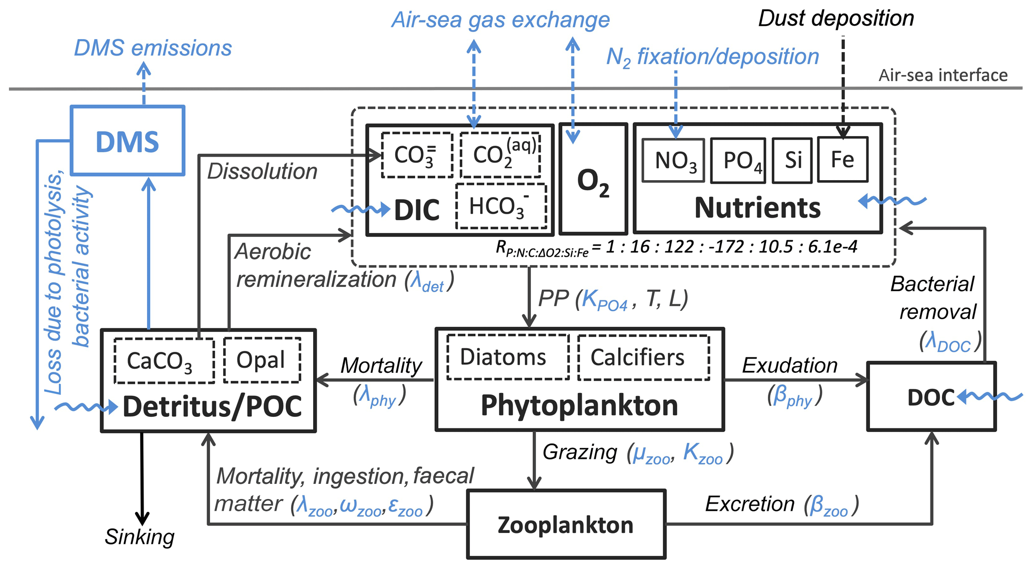
Figure 1Schematic diagram of the ecosystem module in the ocean biogeochemical component of the NorESM2 model. The diagram is an updated version of a similar diagram in Six and Maier-Reimer (2006). Blue depicts components, processes, and parameters that have been modified in NorESM2 relative to the previous model version NorESM1. Dashed arrows indicate air–sea interactions, while wavy arrows depict riverine inputs.
In NorESM1, biological productivity was computed only for the top 100 m of depth, which presumably represents the averaged euphotic layer. In an isopycnic model, there is no static interface separating this depth level. In cases in which the bulk MLD extends below 100 m, we virtually split this at 100 m, and the biological production is simulated only down to this interface. In NorESM2, we have omitted this virtual layer splitting, and the biological production is allowed to occur below 100 m as long as it is within the bulk mixed layer depth and has sufficient light (attenuated with depth and chlorophyll concentration) for phytoplankton growth.
3.1 Preformed tracers
Four new preformed tracers have been implemented in NorESM2, namely preformed dissolved oxygen (), phosphate (), alkalinity (ALKpre), and dissolved inorganic carbon (DICpre). They are initialized to zero at the beginning of the spin-up. During the model integration, in the bulk mixed layer of the model (i.e. the top two levels), the preformed tracers are set to the respective total, non-preformed values at each time step. Below the mixed layer, the preformed tracers are advected as passive tracers by the physical processes and are hence a measure of transport-induced (e.g. circulation, ventilation, etc.) changes. The preformed tracers are included for diagnostic purposes, such as identifying the sources of model–data misfits (Duteil et al., 2012). The preformed oxygen can be used to quantify the total and apparent oxygen utilization (TOU and AOU) as well as O2 disequilibrium (ΔO2) in the interior ocean (Eqs. 10–11; Ito et al., 2004):
and
Here, saturated oxygen () is determined as a function of temperature and salinity (Garcia and Gordon, 1992). Due to its closed coupling with ocean circulation, the preformed oxygen can be used to separate biologically from physically induced biases in the simulated interior biogeochemical tracers.
Following Bernardello et al. (2014), is used to quantify the organic biologically mediated carbon pump (soft tissue, DICsoft), whereas both and ALKpre are used to quantify the inorganic (carbonate, DICcarb) biologically mediated carbon pump (Eqs. 12–14). We use a stoichiometry ratio of in the model such that DICsoft represents remineralized particulate and dissolved organic materials, and DICcarb represents the dissolution of particulate calcium carbonate in the water column:
and
Equation (14) is slightly different from that of Bernardello et al. (2014); i.e. it uses the term instead of rN:P because, in our updated code, we do not neglect the contribution of phosphate to alkalinity changes during biological production and remineralization. For instance, both nitrate and phosphate produced during organic remineralization increase the concentration of proton and therefore reduce the alkalinity (see also Sect. 3.1.3 of Paulmier et al., 2009).
The difference between total DIC and biologically altered DIC (DICsoft + DICcarb, or the biological carbon pump) therefore represents the physical carbon pump (DICpre), which comprises saturated and disequilibrium components (Eq. 15). Here, a tracer of saturated DIC (DICsat) has been implemented. It is computed at the surface layer as a function of atmospheric pCO2, total alkalinity, sea surface salinity (SSS), and sea surface temperature (SST). Below the first layer, DICsat is treated as a passive tracer advected by the circulation. Since the equilibration timescale of the air–sea CO2 fluxes is typically longer than the surface water mass residence time (e.g. in the deepwater formation regions), a disequilibrium term (DICdiss) is computed by subtracting the saturated from the preformed DIC components. The DIC disequilibrium component is used to diagnose the importance of ventilation variability in the physical solubility pump and in the overall DIC storage (Eggleston and Galbraith, 2018):
3.2 Natural inorganic carbon tracers
In order to comply with the Ocean Model Intercomparison Project (OMIP) of CMIP6 (Orr et al., 2017), we have implemented a natural tracer of DIC (DICnat), which is formulated in the same manner as DICtot, except that the air–sea gas exchange is computed with a fixed pre-industrial atmospheric CO2 concentration of 284.32 ppm. In a transient simulation with increasing atmospheric CO2 concentrations, the difference between DICtot and DICnat represents anthropogenic DIC (DICant):
The inclusion of a DICnat tracer also requires the implementation of respective “natural” components for both the alkalinity and the particulate inorganic carbon (CaCO3) tracers. This is because the anthropogenic CO2 uptake alters the carbonate system and therefore the dissolution of CaCO3. We note that anthropogenic carbon does not influence the biological production (e.g. nutrient concentrations and phytoplankton growth rate) in our model. Similarly, a natural air–sea CO2 flux has been added to the model output. These natural tracers are only activated in simulations with atmospheric CO2 that departs from the pre-industrial value. Here, DICnat, TALKnat, and are initialized in the same manner as DIC, TALK, and CaCO3, respectively. In transient historical and future scenario simulations, these tracers provide insight into the natural carbon evolution under anthropogenic climate change.
In addition, DICnat also provides a more precise estimate of DICant entering the ocean since the pre-industrial period than simply taking the difference between DICtot at a specific time and its pre-industrial mean value. Alternatively, these natural tracers could be computed with a parallel transient simulation but with fixed pre-industrial atmospheric CO2 as the ocean carbon cycle boundary condition. The inclusion of natural tracers saves substantial computational time, especially for high-resolution simulations. We note that the DICnat tracer has not been implemented in the sediment module. Hence, in very long-timescale transient simulations in which the sediment changes become substantial, the DICnat tracer may include some uncertainties.
3.3 Carbon isotopes
The 13C and 14C carbon isotope tracers have now been implemented in NorESM2. Naturally occurring stable carbon isotopes (12C, 13C, and 14C) and their relative abundances provide valuable information about both past and present climate. Changes in the 13C:12C ratio are used e.g. to (i) study glacial–interglacial atmospheric CO2 changes from ice core air samples (Broecker and McGee, 2013; Bauska et al., 2016), (ii) reconstruct bottom water oxygen concentrations (Hoogakker et al., 2015), (iii) reconstruct paleo-deepwater circulation (Toggweiler, 1999; Curry and Oppo, 2005; Crucifix, 2005), (iv) investigate oceanic anthropogenic CO2 uptake involving the Suess effect (Gruber and Keeling, 2001; Quay et al., 2003; Holden et al., 2013), and (v) evaluate model sensitivity and performance (Braconnot et al., 2012; Schmittner et al., 2013). The 14C:12C ratio is used as a circulation and age tracer (e.g. Skinner et al., 2017). Globally, the isotope ratio is about . In order to allow for comparison between different carbon isotope studies, the 13C:12C ratio is standardized and expressed in per mille as δ13C (Eq. 24) (Zeebe and Wolf-Gladrow, 2001). Our implementation of 13C follows the OMIP guidelines (Orr et al., 2017). The 14C is standardized as Δ14C (see Sect. 3.3.3). Variations in δ13C are due to isotopic fractionation processes during air–sea gas exchange, photosynthesis, and CaCO3 formation, but the latter is neglected in our implementation (see also Sect. 3.3.2). For 14C, each fractionation factor is the quadratic of the respective 13C value (i.e. κ14C=κ13C2). Lastly, 14C is radioactive and decays with a half-life of 5730 years to 14N following
where
X represents any 14C state variable. In the model, all 14C tracers are normalized to prevent numerical errors from carrying values close to the precision of the model.
The newly implemented marine carbon isotope code parallels the respective total DIC code, and in addition includes fractionation during photosynthesis and air–sea gas exchange (as well as decay for the 14C tracers). In addition to the dissolved inorganic tracers, the following 13C and 14C state variables have also been implemented: dissolved organic carbon, particulate organic carbon, calcium carbonate, phytoplankton, and zooplankton. Therefore, 12 new tracers are added (isotopic DOC, POC, CaCO3, zooplankton, and phytoplankton). Due to the long equilibration time, the isotopic tracers are only activated in the computationally efficient configurations, such as the ocean carbon cycle stand-alone configuration (NorESM2-OC) or the low-resolution version of the coupled model. Equilibrium times of the carbon isotopes are long due to the slow air–sea gas equilibration (Broecker and Peng, 1974) and long-term transient effects from the balance between sediment burial and weathering (Roth et al., 2014). Realistic equilibration times are therefore currently only obtained when bypassing the sediment module of the model when running the carbon isotopes, as well as omitting carbon isotope input from rivers. When bypassing the sediment, mass balance is maintained by redistributing POC fluxes to the sediment over the entire overlying water column and by dissolving inorganic carbon fluxes and opal fluxes at the bottom of the model immediately. Ongoing work will add the possibility for a fast sediment spin-up for use in future versions of the biogeochemical ocean model. Since Δ14C is governed mainly by radioactive decay and circulation, we focus on δ13C in our description of isotopic fractionation effects (Sect. 3.3.1 and 3.3.2).
3.3.1 Air–sea gas exchange fractionation
During air–sea gas exchange, the lighter 12C isotope preferentially escapes to the atmosphere. This fractionation process increases δ13C of surface ocean DIC, although the local net effect depends on the interplay between the local thermodynamic air–sea disequilibrium, the air–sea gas exchange rate, and the strength of the fractionation (Schmittner et al., 2013; Morée et al., 2018). The air–sea fractionation is a function of temperature (T – ∘C) and fraction (fCO3) such that fractionation increases with decreasing temperatures, resulting in higher δ13C in colder than in warmer surface water (Zhang et al., 1995). Fractionation during air–sea gas exchange, which varies between ∼8 and 10.5 ‰, is due to the combined effects of (1) the fractionation between CO2 and the different carbon species, , (2) kinetic fractionation, αk, and (3) fractionation during gas dissolution, . The net air–sea 13CO2 flux is formulated as follows:
Any fractionation αi in Eq. (19) can be expressed as ‰, where
and
In Eq. (19), kw represents the gas transfer velocity for CO2 according to Wanninkhof (2014), and T is in degrees Celsius.
3.3.2 Biological fractionation
Phytoplankton prefers the lighter (12C) isotope during photosynthesis, thereby increasing δ13C of DIC in the surface ocean and producing low-δ13C POC. In the interior ocean, the low-δ13C POC is released back into the water column during remineralization and respiration, though without fractionation (Laws et al., 1995; Sonnerup and Quay, 2012). The “biological isotope pump” thus creates a gradient of higher surface water δ13C and lower deepwater δ13C. The average fractionation during photosynthesis is approximately 19 ‰ (Lynch-Stieglitz et al., 1995; Tagliabue and Bopp, 2008). Even though many relationships for biogenic isotope fractionation have been proposed (e.g. Rau et al., 1996; Keller and Morel, 1999; Popp et al., 1998), modelled δ13C distributions are not very sensitive to the different parameterizations, especially not in the surface ocean (Schmittner et al., 2013; Jahn et al., 2015). In addition, some relationships may be unsuitable for global-scale modelling applications due to the dependency on unknown parameters (e.g. specific species, cell size, and cell membrane permeability).
A parameterization by Laws et al. (1997) is chosen in NorESM2, wherein the biological fractionation ϵbio depends on the ratio between phytoplankton growth rate μ (d−1) at every model time step and the aqueous concentration (µmol kg−1):
The growth rate μ is the gross growth rate, uncorrected for losses such as mortality and exudation. ϵbio increases with increasing and decreasing μ. Fractionation values are kept within a realistic range of 5 ‰–26 ‰ to correct for the influence of extremes (similarly as done by Tagliabue and Bopp, 2008). This non-linear parameterization of Laws et al. (1997) as described in Eq. (23) is preferable over the linear formulation by Laws et al. (1995) because the linear formulation could result in unrealistic fractionation at high growth rates. Isotope equilibrium fractionation during CaCO3 formation increases δ13C of CaCO3 and therefore depletes seawater of 13C (thereby lowering seawater δ13C). Nevertheless, the fractionation effect during CaCO3 formation is relatively small (i.e. of the order of −2 ‰ to +3 ‰, depending on species and environmental conditions; Grossman and Ku, 1986; Ziveri et al., 2003; Zeebe and Wolf-Gladrow, 2001) compared to the effects of air–sea gas exchange and photosynthesis. Therefore, fractionation during CaCO3 formation is commonly omitted in modelling studies (e.g. Lynch-Stieglitz et al., 1995; Schmittner et al., 2013). There are additional uncertainties related to temperature and species dependencies (Grossman and Ku, 1986; Zeebe and Wolf-Gladrow, 2001). Taking this into consideration, we have chosen not to implement fractionation during CaCO3 formation in NorESM2.
3.3.3 Diagnostic and initialization
In order to evaluate the carbon isotopes against observations, we compute the diagnostic variables δ13C and δ14C according to their standard formulations, as follows:
and
where (13C∕12C)PDB is the established Pee Dee Belemnite standard ratio of 0.0112372, and NBSstd is (Orr et al., 2017). The DI12C is computed as the difference between total DIC and DI13C.
In the model, the initialization of the carbon isotope tracers is done as follows: first, the model is spun up with pre-industrial boundary conditions until the non-isotope carbon chemistry reaches a quasi-equilibrium state. Next, we compute DI13C initial values by solving Eq. (24) for 13C using the simulated AOU and DIC together with the δ13C:AOU relationship reported by Eide et al. (2017), i.e. . The DI14C is initialized by first calculating δ14C by solving Eq. (26) using pre-industrial δ13C from Eide et al. (2017) (with the missing upper 200 m copied from the 200 m depth values) and the observationally based estimate of pre-industrial Δ14C (Key et al., 2004). This δ14C is then converted to absolute model DI14C using Eq. (25). The remaining isotope tracers are initialized as , with C as the total carbon counterpart of the respective isotope tracer, R as the DI13C∕DI12C or DI14C∕DI12C ratio, and ζ=0.98, a typical value for biological fractionation (applied to organic carbon components only).
Here, the prognostic atmospheric pCO2 was initialized at 278 ppm from the start of the simulation. At initialization of the carbon isotopes, atmospheric δ13C and Δ14C are set to −6.5 ‰ and 0 ‰, respectively. Lastly, the results are presented as calibrated Δ14C to account for long-term drift. That is, DI14C is multiplied with a factor F before standardization to DI14C corresponding to an atmospheric Δ14C of 0 ‰ (14Catmzero).
where 14Catm in our simulation is found from the pre-calibrated Δ14Catm of approximately 36 ‰, and 14Catmzero is likewise determined by solving Eqs. (25) and (26) for Δ14C=0 ‰, in both cases using model δ13Catm (−7.5 ‰) and atmospheric pCO2 (294 ppm). This leads to %.
Due to the long timescale of the large-scale ocean thermohaline circulation (flushing time is of the order of 1000–1500 years), a sufficiently long model integration of the order of at least 1000 years is required to achieve a quasi-equilibrium biogeochemical state in the interior ocean (Séférian et al., 2016). Prior to running any transient simulations, we have spun the model up for 1200 model years in a fully coupled configuration so that the ocean biogeochemistry reaches a quasi-equilibrium state. In the spin-up simulation, all boundary conditions are fixed to constant pre-industrial values, following the CMIP6 protocols (Eyring et al., 2016a). Due to the oceanic DMS fluxes, there is an internal feedback between the ocean biogeochemistry and the atmospheric radiative forcing during the spin-up. The end of the model spin-up is used as a starting point for (1) the pre-industrial control simulation (piControl, years 1850–2349), (2) transient historical simulation (years 1850–2014), and (3) esm-piControl-spinup simulation (100 model years). The end of simulation (3) is furthermore used as a starting point for (3a) an esm-piControl simulation (for 250 years) and (3b) a transient esm-hist (years 1850–2014) simulation. The use of the prefix esm- (i.e. in experiments 3, 3a, and 3b) follows the CMIP6 naming convention (Eyring et al., 2016a), which indicates emission-driven simulation in which the atmospheric CO2 is prognostically computed from ocean–atmosphere and land–atmosphere CO2 fluxes, as well as from prescribed anthropogenic emissions (for esm-hist). Here, the atmospheric CO2 is transported by the atmospheric circulation model. In the esm-piControl-spinup the atmospheric CO2 concentration is relatively stable, with a small drift of −0.002 ppm yr−1 and a long-term mean of 280.6±0.4 ppm.
Except for the carbon isotopes (see next paragraph), all analyses shown in this paper were extracted from the two transient historical simulations (prescribed CO2-historical and prognostic CO2-esm-hist). Since both simulations produce nearly identical climatology states, we only present results from the prescribed CO2-historical simulation.
For the newly implemented carbon isotopes, a considerably longer spin-up is required. Therefore, the carbon isotope tracers were not activated in our fully coupled simulations. Instead, simulations with carbon isotopes switched on have been performed using the ocean carbon cycle stand-alone configuration of NorESM2. Additionally, a lower-resolution ocean grid (using a similar tripolar grid as described above but with a nominally 2∘ resolution) has been used. This configuration avoids the high computational cost of running a long spin-up in a fully coupled configuration. The atmospheric forcing of the spin-up is the CORE normal-year forcing (Large and Yeager, 2004), which represents a climatological mean year with a smooth transition between the end and start of the year. Atmospheric CO2, 13CO2, and 14CO2 concentrations are kept track of with a box atmosphere (i.e. assuming 100 % instant mixing), which is updated each time step according to the modelled air–sea CO2 fluxes using a conversion factor of 2.13 ppm Pg C−1. These simplified prognostic atmospheric fields are simulated from the start of the spin-up (and the subsequent start of the carbon isotope simulation). As mentioned above, we have not implemented the carbon isotopes in the sediment compartment of the model. Therefore, the sediment module of iHAMOCC was switched off for the carbon isotope simulations presented here. Otherwise, the setup of the ocean carbon cycle stand-alone configuration is as described in Schwinger et al. (2016). The model spin-up was run for 5000 years, the first 1000 years of which were run without carbon isotopes. At year 1000 (4000), after the largest transient changes in biogeochemical tracers have flattened out, we initialized the 13C (14C) tracers as described above. At the end of year 5000, the model reaches a quasi-equilibrium state, which approximately corresponds to the pre-industrial state. Here, we evaluate the simulated carbon isotope simulations against the pre-industrial estimates of the respective tracers.
Here, we evaluate the model performance in simulating the mean climatological state of key biogeochemical tracers and the evolution of air–sea CO2 fluxes from the transient historical and esm-hist simulations. The carbon isotope results are from a stand-alone ocean simulation.
5.1 Statistical performance summary
We assess, relative to the observational estimates and the earlier version NorESM1, the simulated long-term annual mean of global hydrography and biogeochemical tracer distributions. Where relevant, the mean seasonal cycles are also evaluated for the surface values. The list of parameters, the averaging periods, and the respective observational data used to assess the model performance are given in Table 2. We use spatial correlation and normalized RMSE (root mean squared error) metrics to measure the model–data difference and determine whether or not the current model version has improved and performed better than the earlier version. The normalization was done by dividing the RMSE with the standard deviation of the respective observations.
(Locarnini et al., 2013)(Zweng et al., 2013)de Boyer Montégut et al. (2004)(Garcia et al., 2013a)(Garcia et al., 2013b)(Garcia et al., 2013b)(Garcia et al., 2013b)(GLODAPv2; Lauvset et al., 2016)(GLODAPv2; Lauvset et al., 2016)Landschützer et al. (2015)Landschützer et al. (2015)(Behrenfeld and Falkowski, 1997; Westberry et al., 2008)Lana et al. (2011)Key et al. (2004)Eide et al. (2017)Key et al. (2004)Table 2List of the simulated variables and the respective historical simulation periods over which their climatological values have been averaged. The last column indicates the observational reference used to validate the model output.
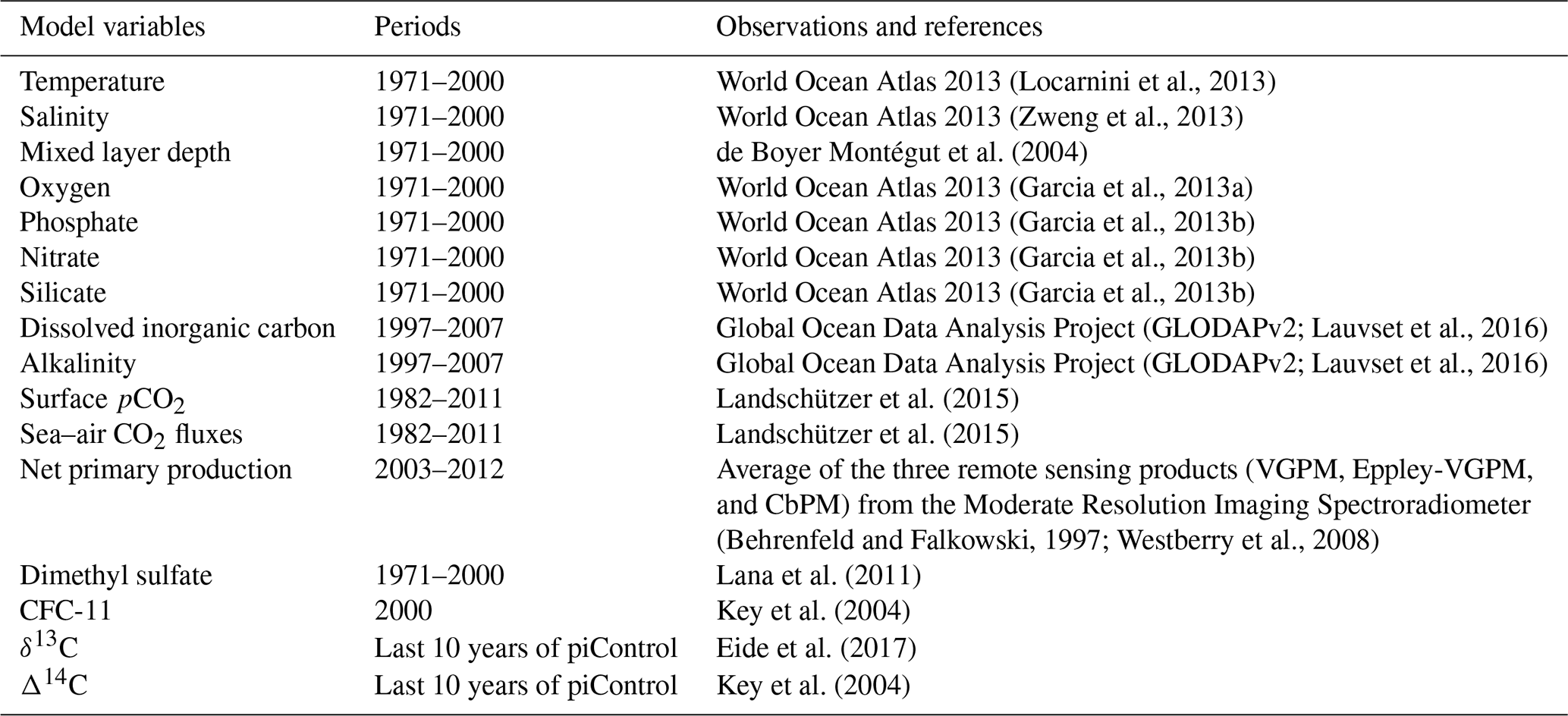
Figure 2b shows that, except for the surface layer, the NRMSE of most of the NorESM2 variables' mean climatology is either noticeably improved or relatively similar to that of NorESM1. At 500 m of depth, all variables but salinity have lower RMSE values. For many of the biogeochemical tracers (phosphate, nitrate, oxygen, and DIC), NorESM2 shows better agreement with data throughout the water column. Similarly, the respective spatial correlations with the observations are considerably improved for most variables, especially for nitrate, DIC, and alkalinity (Fig. 2a). For surface seasonality, NorESM2 performs fairly comparable to NorESM1, with improvements in all seasonal metrics (NRMSE and spatial pattern) for surface salinity and net primary production. NorESM2 simulates slightly larger NRMSE in its surface nutrients (phosphate, nitrate, and silicate) for both their annual and seasonal average values relative to NorESM1. This is attributed to the anomalously high concentration in the Arctic Ocean and parts of the Southern Ocean (just north of the Antarctic Circumpolar Current). More details on the performance of each specific variable are discussed in the following subsections.
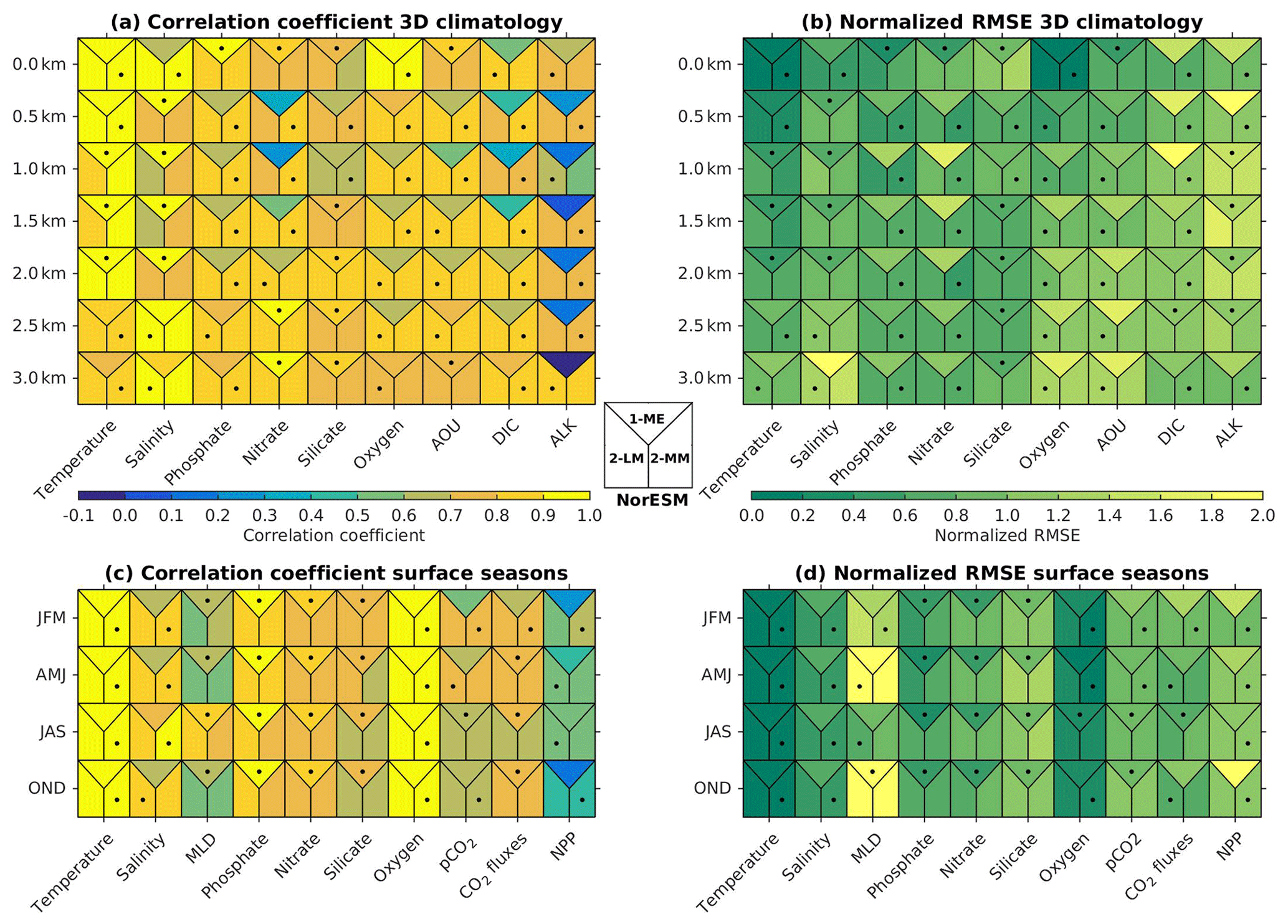
Figure 2Summary of (a, c) spatial correlation coefficients and (b, d) normalized RMSE between the observations and models (NorESM1-ME, NorESM2-LM, and NorESM2-MM). In all (a, b) 3D fields, the metric values are computed over a 2D horizontal global domain ranging from the surface to 3 km of depth, while for (c, d) seasonal metrics, only surface values are evaluated. Each square contains three metric scores, i.e. for NorESM1-ME (top), NorESM2-LM (bottom-left), and NorESM2-MM (bottom right). Black dots indicate which model performs the best.
5.2 Temperature
NorESM2 simulates a warm bias for both pre-industrial conditions and the contemporary surface ocean (Fig. 3d), where a warm bias as high as 5 ∘C is simulated in some regions of the Southern Ocean. Cold biases are simulated in parts of the north and equatorial Pacific, North Atlantic subpolar gyre, and the Arctic Ocean. The climatological mean temperatures are broadly similar between the two NorESM versions, with NorESM2 having fewer spatial correlations at 1 and 1.5 km depths (Fig. 2a, b). At depths below 2 km, with the exception of the North Pacific, NorESM2 simulates fewer biases (Fig. 3e, f, h, i). This improvement is related to the more accurately simulated Antarctic Bottom Water (AABW; see also Supplement Fig. S1) in both the Pacific and Atlantic basins, as also depicted in Fig. 3. While NorESM1 simulates an AMOC strength that is too strong (roughly 31 Sv at 26∘ N), NorESM2 has a more reasonable strength of approximately 21 Sv. Nevertheless, the warm bias of 1–2 ∘C in the North Atlantic Deep Water (NADW) remains when compared to observations. The cold bias seen previously in the intermediate water mass in the Southern Ocean and North Pacific has been improved in the new version. In the Atlantic sector just south of 30∘ N at 1 km of depth, there is a warm bias of up to 5 ∘C (Fig. 3e), which could be related to the anomalously strong overflow water mass from the Mediterranean Sea. Nevertheless, the cold bias in the Atlantic and Pacific tropical–subtropical thermocline simulated in NorESM1 is now improved in NorESM2. Temperature values from NorESM2-LM are shown in Supplement Fig. S2.
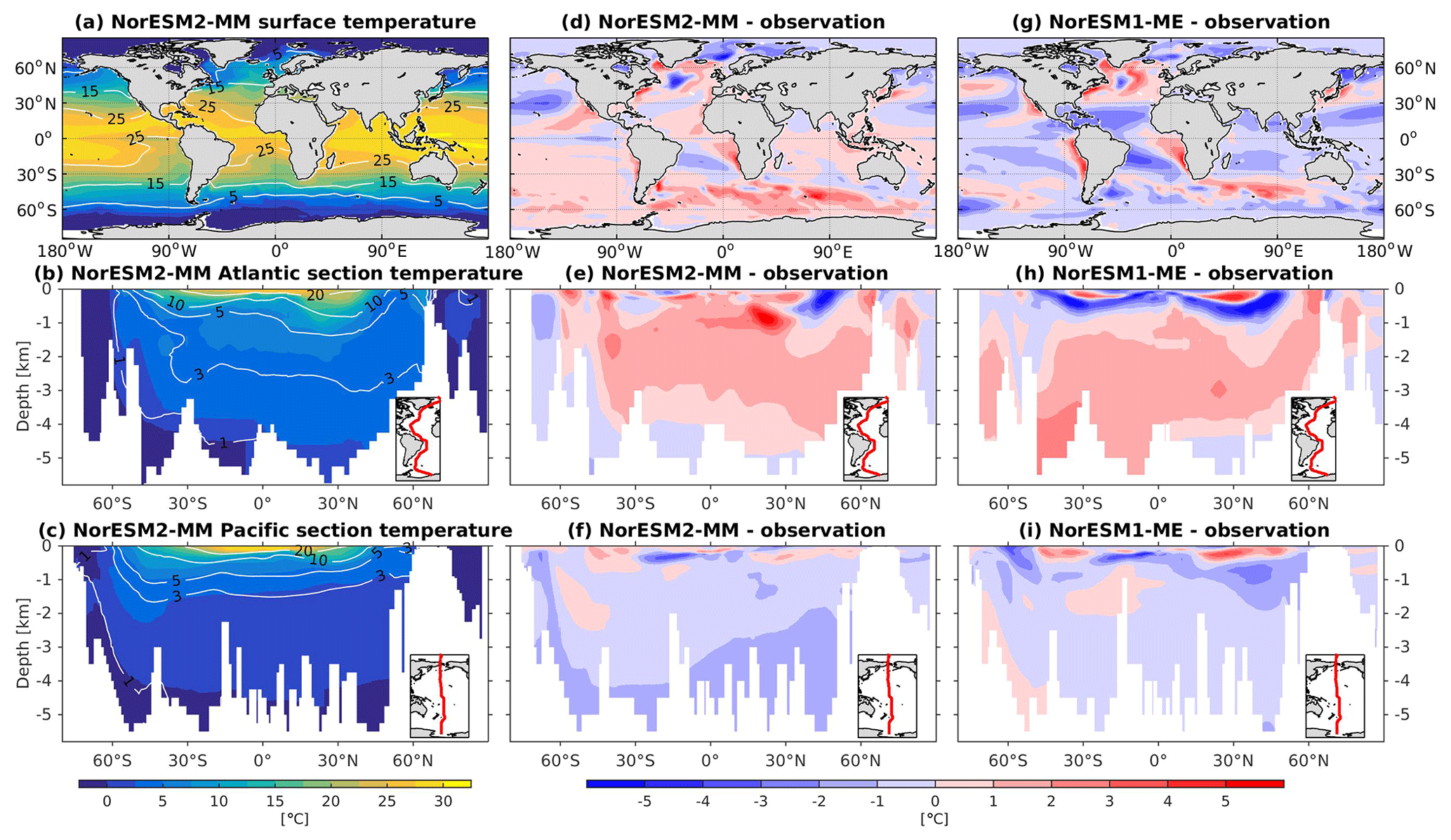
Figure 3Climatological temperature values at the (a) surface and across the vertical sections of (b) the Atlantic and (c) Pacific in NorESM2-MM (colour shadings) and from observations (contour lines). Differences between NorESM2-MM (or NorESM1-ME) and observations are shown in panels (d)–(i).
5.3 Salinity
The RMSE in surface salinity is reduced in NorESM2, mostly owing to improvements in the Arctic, where the previous model version simulates water that is too saline (Fig. 4d, g). Also at the surface, NorESM2 simulates biases that are anomalously too fresh and too saline in the Pacific and the Atlantic basins, respectively. In the subtropical South Pacific, the negative bias is as high as −2 psu and is consistent with a precipitation rate that is too strong in this region simulated by the atmospheric component (not shown). Positive biases are simulated in the northern Indian Ocean and along the Benguela current extension. In the interior, the salinity bias in the Pacific and the Atlantic is of the order of ±0.11 and +0.4 psu, respectively (Fig. 4e, f). In the NADW, NorESM2 displays a positive bias, which is, however, smaller than that of NorESM1 (Fig. 4h; bias greater than 0.5 psu). Similar to temperature bias, NorESM2 produces too much saline water around 30∘ N at 1 km of depth in the Atlantic (Fig. 4e) due to overflow of high-salinity Mediterranean water masses. In the interior Pacific and Southern Ocean, both models' performances are generally comparable (Fig. 4e, f, h, i). Except for the surface salinity, the simulation with lower atmospheric resolution (NorESM2-LM) depicts a similar salinity pattern throughout the water column (Supplement Fig. S3).
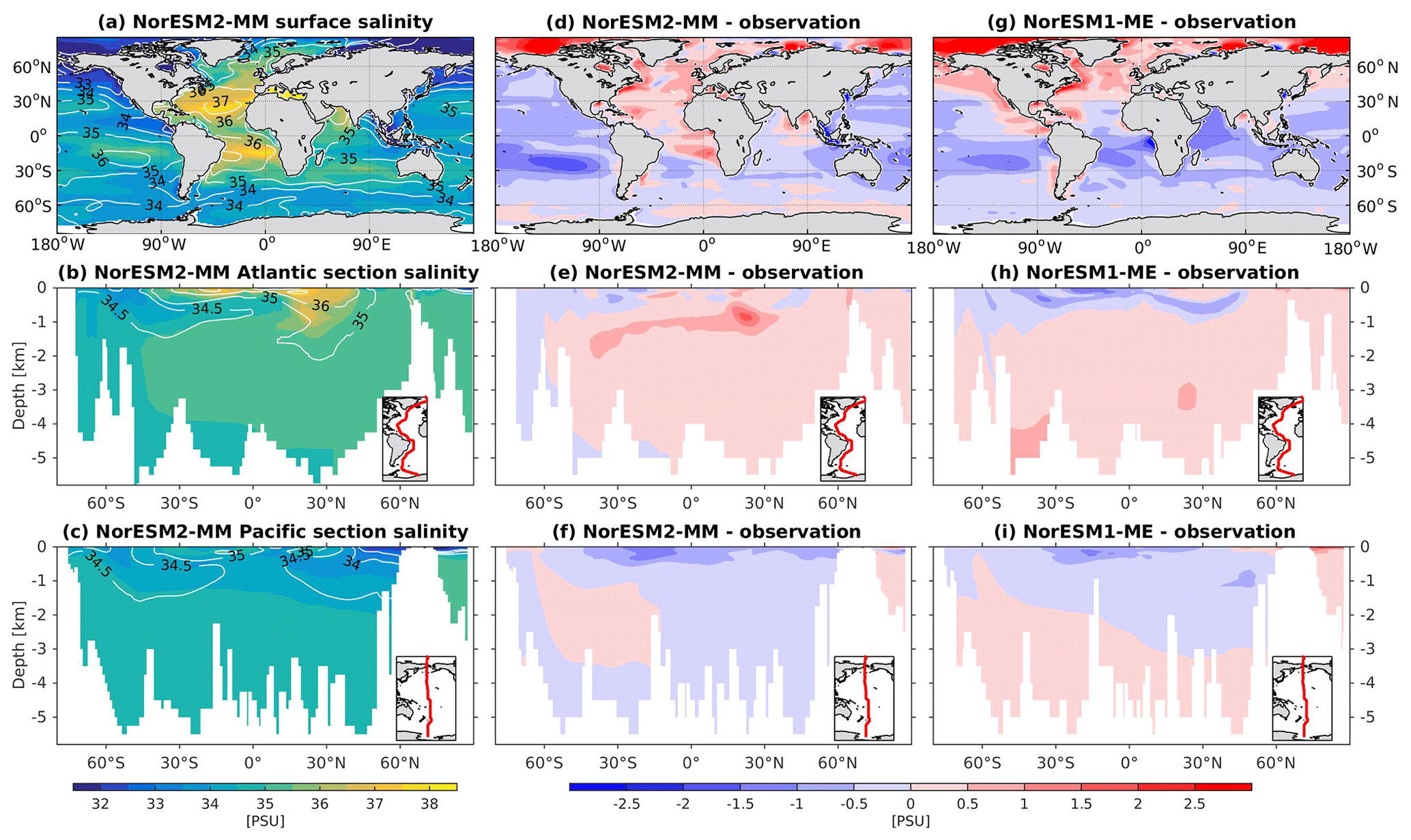
Figure 4Climatological salinity values at the (a) surface and across the vertical sections of (b) the Atlantic and (c) Pacific in NorESM2-MM (colour shadings) and from observations (contour lines). Differences between NorESM2-MM (or NorESM1-ME) and observations are shown in panels (d)–(i).
5.4 Mixed layer depth
Seasonally averaged mixed layer depths (MLDs) from NorESM2 and observations are shown in Fig. 5. To be consistent with the observational estimates (de Boyer Montégut et al., 2004), we have computed our MLD using the σT (density) criteria, which is the first depth at which the change from surface σT of 0.03 has occurred. In NorESM1, the MLD is generally too deep throughout most ocean regions. The new improvements in the MLD parameterization in NorESM2 reduce this bias considerably, especially in the low and middle latitudes as well as the North Pacific regions. In the subpolar North Atlantic and parts of the Southern Ocean, the simulated MLD is still deeper than the observation-based estimates. In the Weddell Sea, NorESM2 also persistently simulates a deep MLD throughout the year, a feature not seen in the observations. There is no significant difference between MLD simulated in NorESM2-MM and NorESM2-LM (Supplement Fig. S4).

Figure 5Climatological seasonal mixed layer depth as (left column) simulated in NorESM2-MM and (right column) estimated from observations.
5.5 Ocean ventilation
To assess the simulated ventilation, we compare the passive chlorofluorocarbon (CFC-11) tracer distribution in the interior Atlantic and Pacific Ocean as simulated by NorESM2 with that from observations, as shown in Fig. 6. We compare the simulated CFC-11 from calendar year 2000 with climatological estimates of Key et al. (2004). Similar to the observations, high values of CFC-11 are generally simulated in the upper 1 km in both the Atlantic and the Pacific, with the exception of the North Atlantic, where up to 0.5 nmol CFC-11 m−3 penetrates down to 5 km of depth. In the mid-latitude North Atlantic (i.e. 30∘ N), the model is unable to simulate the observed high values at around 1 km of depth. This is likely due to the discrepancy in the water mass origin between the model and observations. Here, the water mass in the model is too old, as also seen in the overly high apparent oxygen utilization and dissolved inorganic carbon (see the subsections below on oxygen and DIC). The model simulates deepwater ventilation that is too strong in both the Atlantic and Pacific sectors of the Southern Ocean as well as in the high latitudes of the North Atlantic. Similar ventilation patterns are also produced by NorESM2-LM (Supplement Fig. S5), with slightly less ventilated North Atlantic.

Figure 6Concentration of CFC-11 across the vertical sections of (a) the Atlantic and (b) Pacific from NorESM2-MM (colour shadings) and observations (contour lines). Differences between NorESM2-MM and observations are shown in panels (c)–(d).
5.6 Nutrients
In general, the climatological nutrient distributions (phosphate, nitrate, and silicate) in NorESM2 are either comparable or improved compared to those of NorESM1 in both spatial correlation and normalized RMSE (Fig. 2a, b). At depth, these improvements are due to the new particulate organic carbon sinking scheme, whereby the sinking velocity increases linearly with depth. In NorESM1, the sinking speed is constant with depth, leading to more organic material being remineralized in the upper 1.5 km. The sinking scheme in NorESM1 produces anomalously high regenerated phosphate at intermediate depth (approximately between 100 and 1500 m of depth; Fig. 7h, i). A consequence of this is an oxygen minimum zone that is too strong (OMZ; see also the next subsection) and denitrification in the low latitudes, where the nitrate concentration becomes overly depleted. On the other hand, at depths greater than 1500 m, NorESM1 exhibits concentrations of all nutrients that are too low relative to the observations (panels h and i in Figs. 7–9).

Figure 7Climatological phosphate values at the (a) surface and across the vertical sections of (b) the Atlantic and (c) Pacific in NorESM2-MM (colour shadings) and from observations (contour lines). Differences between NorESM2-MM (or NorESM1-ME) and observations are shown in panels (d)–(i).
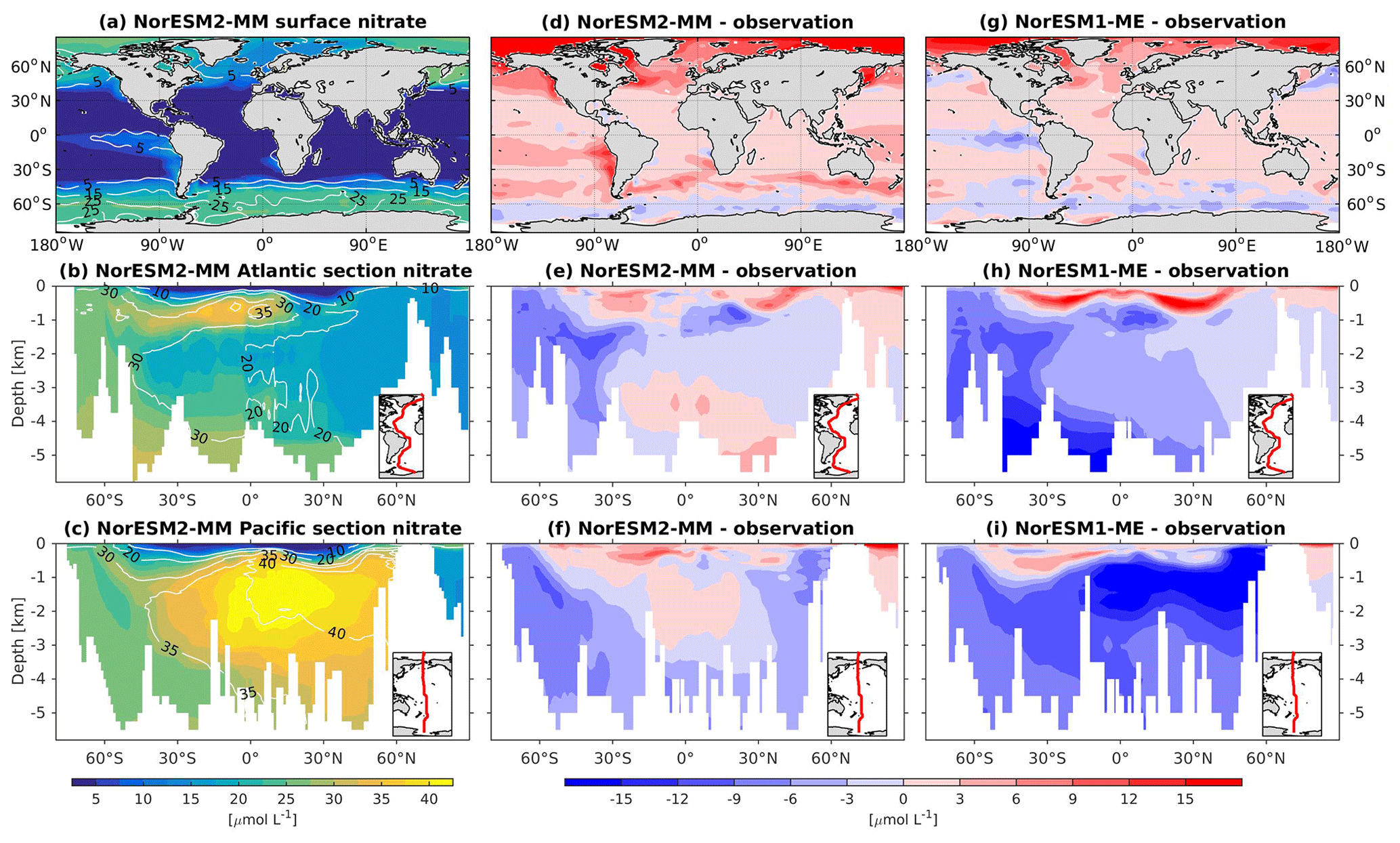
Figure 8Climatological nitrate values at the (a) surface and across the vertical sections of (b) the Atlantic and (c) Pacific in NorESM2-MM (colour shadings) and from observations (contour lines). Differences between NorESM2-MM (or NorESM1-ME) and observations are shown in panels (d)–(i).
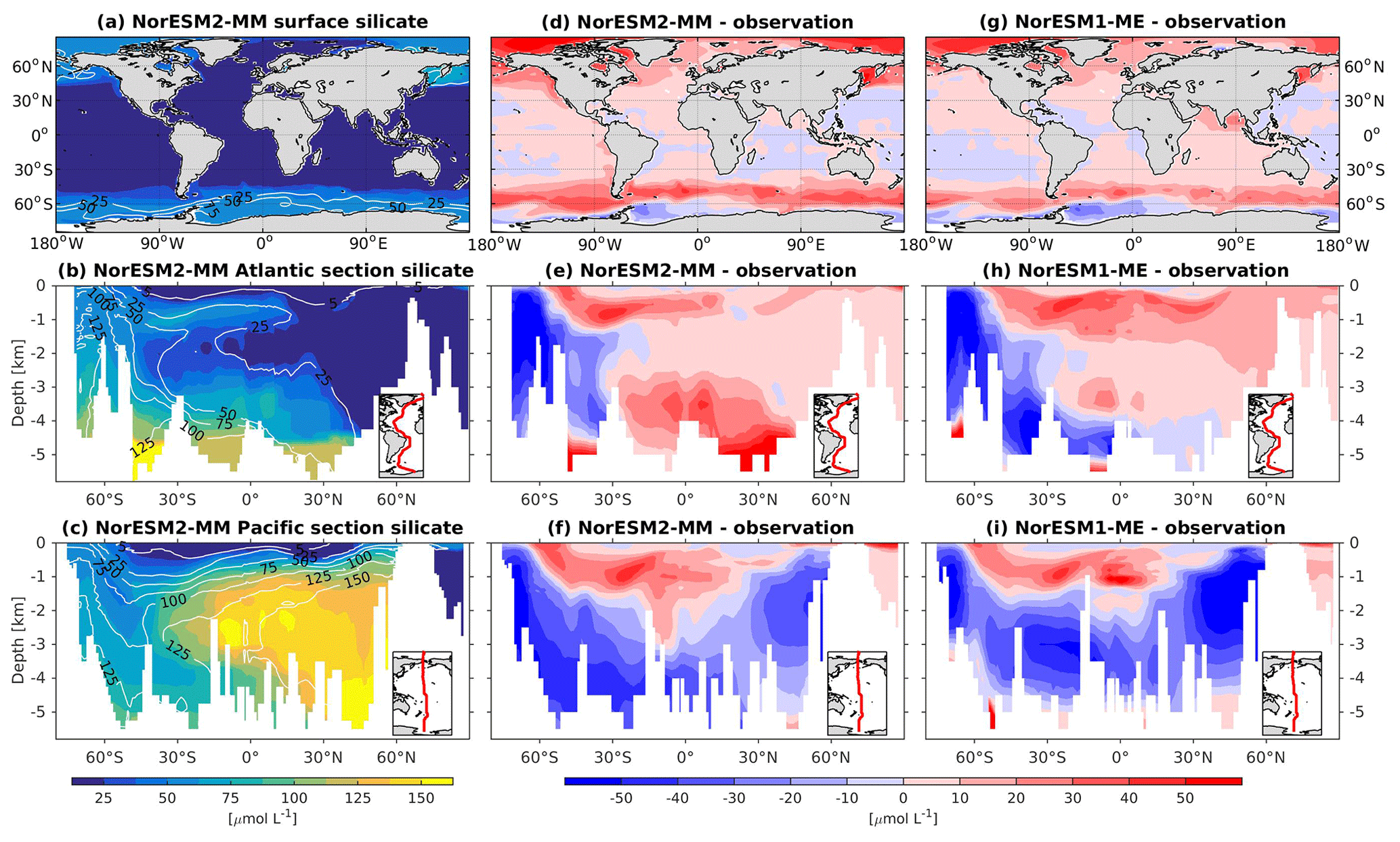
Figure 9Climatological silicate values at the (a) surface and across the vertical sections of (b) the Atlantic and (c) Pacific in NorESM2-MM (colour shadings) and from observations (contour lines). Differences between NorESM2-MM (or NorESM1-ME) and observations are shown in panels (d)–(i).
With the new sinking scheme, more organic material reaches the deep ocean and gets remineralized there. As a result, model–data biases in phosphate and nitrate in the interior are noticeably improved (Figs. 2b, 7e, f, 8e, f). In the Pacific OMZ, reduced export production in NorESM2 also contributes to the reduced nutrient bias. In the interior North Atlantic, despite strong positive spatial correlation with the observations, NorESM2 shows a positive bias at depth below 3000 m and north of 30∘ S (Figs. 7e, 8e, 9e). Through analysing the quasi-conservative “PO” tracer (Broecker, 1974), we are able to attribute this to the bias in the simulated water mass (Supplement Fig. S1). In NorESM2, this region is dominated by Antarctic Bottom Water, whilst the observations indicate NADW as the main water mass. As with NorESM1, the current model still simulates nutrient concentrations that are too low in the North Pacific Intermediate Water mass (Figs. 7f, 8f, 9f). This is likely associated with the excessively low surface primary production simulated in this region (see also Sect. 5.8), leading to limited organic matter available for remineralization at depth. We note that the circulation bias in this region could also contribute to the nutrient bias. In the Southern Ocean, overly strong ventilation potentially leads to negative nutrient biases in both the Atlantic and Pacific sectors.
In NorESM2, less export production and deeper distribution of POC through the changed sinking scheme lead to a reduced rate of denitrification in the Pacific oxygen minimum zone and a greatly improved nitrate distribution (Fig. 8f). In NorESM1, far too much nitrate was consumed for denitrification (Fig. 8i). The silicate spatial distribution in NorESM2 closely resembles the phosphate distribution (Figs. 9a–c and 7a–c), with similar biases across the vertical sections of the Atlantic and Pacific (Figs. 9e, f and 7e, f). At high latitudes, NorESM2 overestimates the surface silicate concentration (Fig. 9d), which could be attributed to the reduced opal export sinking speed relative to our earlier model version (30 instead of 60 m d−1 previously).
In NorESM, the bulk phytoplankton growth rate is limited by multiple nutrients (i.e. phosphate, nitrate, and dissolved iron), in addition to temperature and light (see also Sect. 2.3.2 of Schwinger et al., 2016). The model does not explicitly simulate diatom and calcifier classes. The inclusion of iron is critical to simulate the observed HNLC (high-nutrient low-chlorophyll) regions in the world ocean where year-long elevated concentrations of both nitrate and phosphate are not exhausted by phytoplankton (de Baar et al., 1995; Martin and Fitzwater, 1988). The three major HNLC regions are the subarctic North Pacific, the eastern and central equatorial Pacific, and the Southern Ocean. Here, low levels of bioavailable iron concentrations limit phytoplankton growth. In NorESM1, only the subarctic North Pacific is simulated to be iron-limited, with the other two HNLC regions being mostly limited by nitrate, as shown in Fig. 10. Iron limitation is also incorrectly simulated in parts of the subtropical North Pacific, South Pacific, and most parts of the western Pacific. Following improvements in the iron parameterization, the three HNLC regions are now shown to be iron-limited in NorESM2. Nevertheless, the iron limitation bias in the western equatorial Pacific remains.
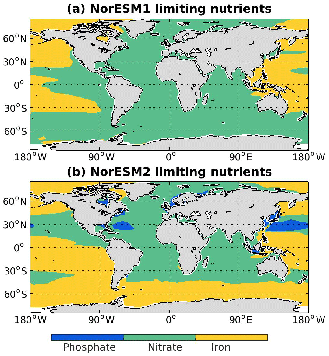
Figure 10Maps of limiting nutrients for biological productivity as simulated in (a) NorESM1 and (b) NorESM2. The limiting nutrient is determined as the minimum between PO4, , and .
5.7 Dissolved oxygen
At the surface level, dissolved oxygen is mostly constrained by solubility and hence sea surface temperature. Both NorESM1 and NorESM2 perform similarly for dissolved oxygen at the surface, with subtle improvements in the seasonal spatial correlation coefficient of NorESM2 (Fig. 2a, c). As with nutrients, the climatological distributions of interior oxygen improved considerably when compared to NorESM1 (Fig. 11), which is one of the CMIP5 ESMs with an overly strong OMZ (Cabré et al., 2015). In NorESM2, the OMZ volume is reduced considerably in both the equatorial Atlantic and Pacific, and the absolute dissolved oxygen values are also much improved (Fig. 11e, f). Here the remaining bias is related to the nutrient trapping issue (Six and Maier-Reimer, 1996), as can also be seen from excessively high apparent oxygen utilization (AOU; Fig. 12d). In the interior Pacific and Atlantic roughly at 2 km and deeper, NorESM2 simulates a considerably higher oxygen concentration than the observations by as much as 50 % (North Pacific Deep Water; Fig. 11f). In the North Pacific Deep Water, this is primarily due to too little organic matter flux reaching below the mesopelagic zone, leading to apparent oxygen utilization that is too low (Fig. 12d). The uncertainty in the dissolved organic carbon (not shown), which is currently not well constrained due to lack of observational data, could also play a role in this. In addition to biological constraints, the remaining interior oxygen bias can be attributed to the overly strong Antarctic Bottom Water (AABW) ventilation, which carries a colder (Fig. 3e, f) and higher oxygen-saturated water mass into both the Atlantic and Pacific bottom waters (Fig. 11e, f).
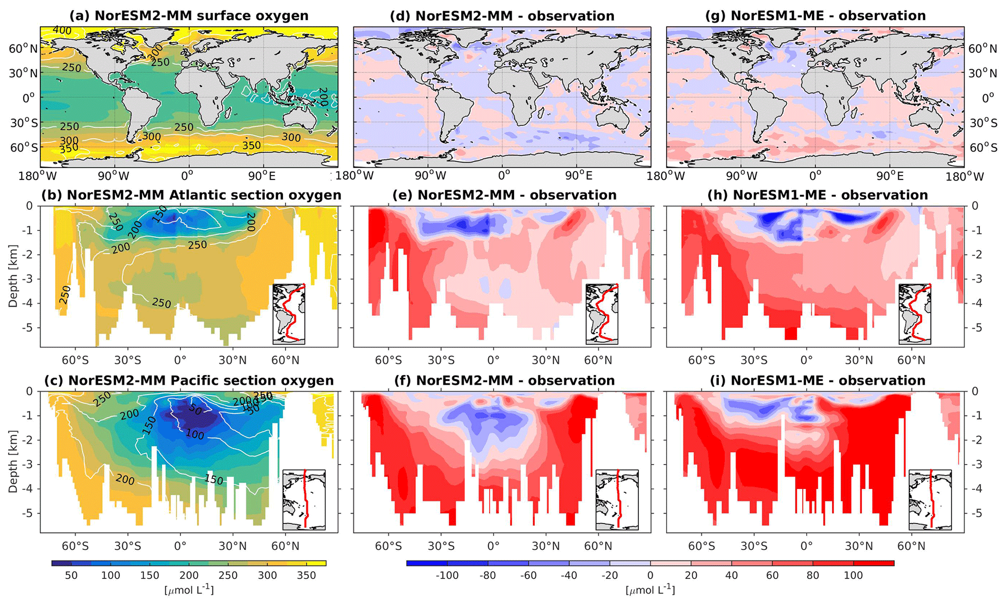
Figure 11Climatological dissolved oxygen values at the (a) surface and across the vertical sections of (b) the Atlantic and (c) Pacific in NorESM2-MM (colour shadings) and from observations (contour lines). Differences between NorESM2-MM (or NorESM1-ME) and observations are shown in panels (d)–(i).
5.8 Biological production
In NorESM1, the primary production is generally too strong in the equatorial Pacific and during the summer months at high latitudes. In the subtropical oceans, the simulated production is too low relative to the observational estimates. With the newly tuned ecosystem parameters of NorESM2, the spatial productivity patterns are improved considerably, with an average absolute bias in the open ocean of less than 5 mol C m−2 yr−1 (Fig. 13a). In NorESM1 these biases reach more than 10 mol C m−2 yr−1, especially in the equatorial Pacific, the South Atlantic, and the Southern Ocean. Seasonally, the spatial patterns are also improved when compared to the observations, with a correlation of approximately r=0.5 (Figs. 2c, 13c). The NRMSE has also been reduced considerably, particularly in the October–November–December months when NorESM1 simulates a spring bloom that is much too strong in parts of the Southern Ocean, which is overestimated by as much as a factor of 8 (e.g. Figs. 13e, 14e and Nevison et al., 2015). Similarly, the spring blooms in the North Atlantic and North Pacific are overestimated in NorESM1 (Figs. 13e, 14a). The improved spring bloom characteristics at high latitudes, however, come at the cost of annual mean productivity that is too low in the North Atlantic and North Pacific.

Figure 12Climatology of apparent oxygen utilization (AOU) values across the vertical sections of (a) the Atlantic and (b) Pacific in NorESM2 (colour shadings) and from observations (contour lines). Differences between NorESM2-MM (or NorESM1-ME) and observations are shown in panels (c)–(f).
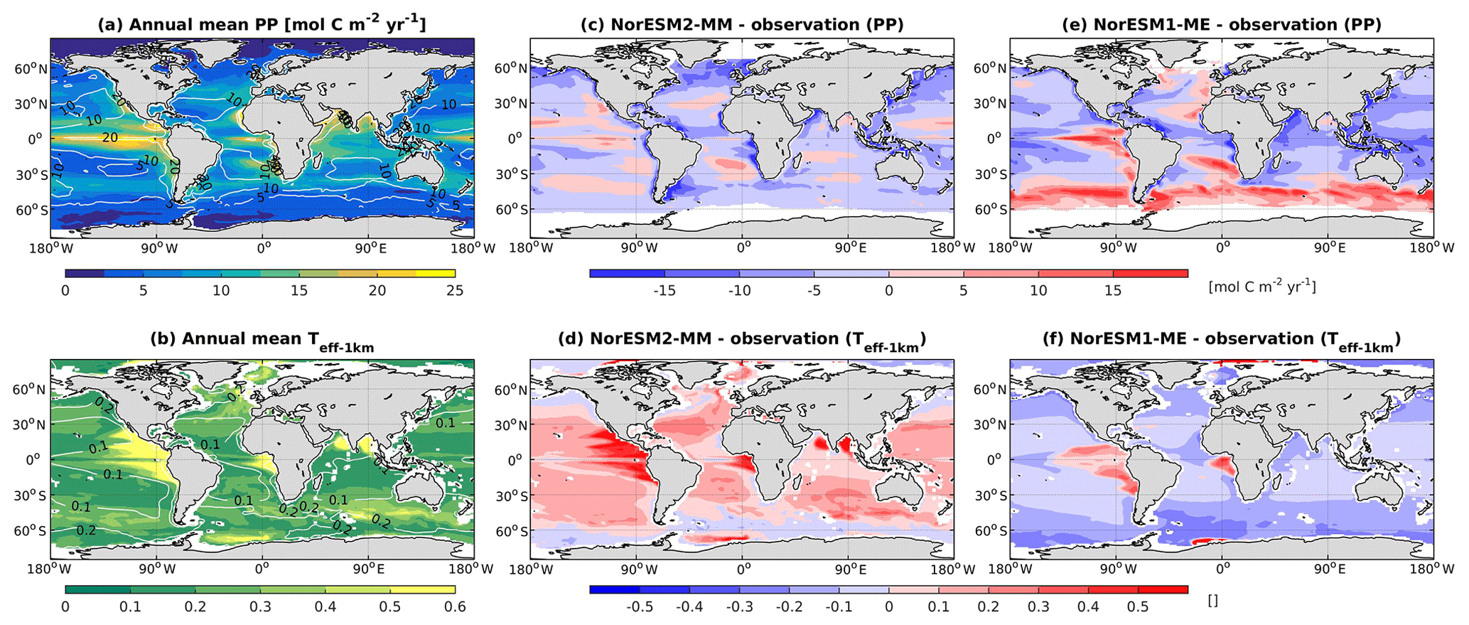
Figure 13Annual mean (a) vertically integrated contemporary primary production and (b) transfer efficiency (Teff-1 km) as simulated in NorESM2 (colour shadings) and from observations (contour lines). Respective difference between NorESM2-MM (NorESM1-ME) and observations are shown as colour shadings (contour lines) in panels (c)–(d).
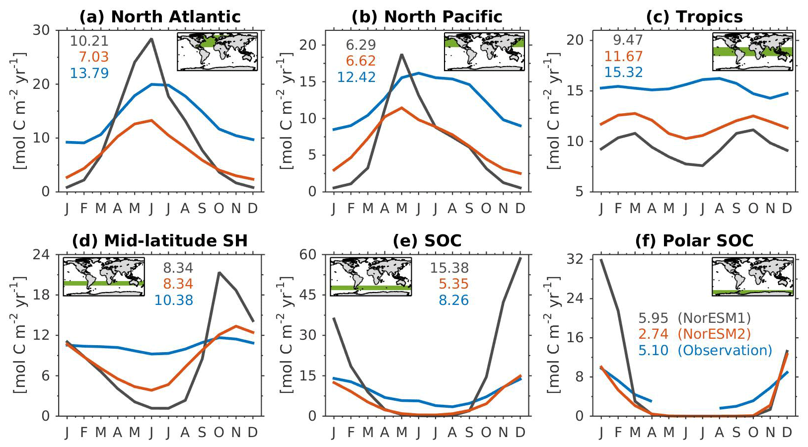
Figure 14Mean seasonal cycle of vertically integrated contemporary primary production in the (a) North Atlantic (north of 20∘ N), (b) North Pacific (north of 20∘ N), (c) tropics (20∘ S–20∘ N), (d) mid-latitude Southern Hemisphere (20∘ S–40∘ S), (e) Southern Ocean (40∘ S–60∘ S), and (f) polar Southern Ocean (south of 60∘ S). Shown are values from NorESM1-ME (black), NorESM2-MM (red), and observational estimates (blue). Numbers within each panel depict the regional mean values averaged over all months.
Due to unresolved physical dynamics, the model is still unable to reproduce the observed high productivity in coastal regions. Globally, the contemporary total primary production in NorESM2 (NorESM1) is 35.3 (39.9) Pg C yr−1. These estimates are lower than the observational (MODIS, excluding coastal areas) estimates of 46.1 Pg C yr−1 but within the broad range of CMIP5 models (Bopp et al., 2013). In our model, export production is estimated as the flux of particulate organic carbon exiting the base of the euphotic zone (here assumed to be 100 m of depth) as a function of zooplankton and phytoplankton mortalities and zooplankton faecal materials. Table 3 shows that the export production in NorESM2 is 5.39 Pg C yr−1 compared to 7.90 Pg C yr−1 simulated by NorESM1. Current estimates of the global export production remain highly uncertain, from 5 to > 12 Pg C yr−1, with a more recent satellite-based approach that accounts for food-web processes revealing values of 6±1.2 Pg C yr−1 (Siegel et al., 2014).
Table 3Annual mean biology-related metrics simulated by NorESM1-ME, NorESM2-LM, and NorESM2-MM.
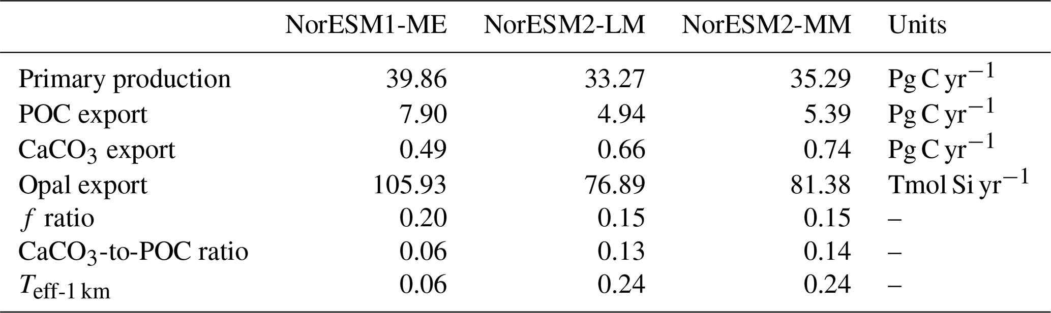
Table 3 also summarizes other export production metrics from both model versions. As a consequence of the new particle sinking scheme, there is more POC exported into the deep ocean. This is especially reflected by the values of transfer efficiency (Teff-1 km), which is calculated as a ratio between POC fluxes at a depth of 1000 and 100 m. The Teff-1 km in NorESM2 (0.24) is increased by a factor of 4 relative to that in NorESM1 (0.06). Compared to a recent estimate of transfer efficiency reconstructed from observed interior biogeochemistry (Fig. 13b; Weber et al., 2016), NorESM2 still simulates transfer efficiencies of >50 % that are too high in the eastern equatorial Pacific (Fig. 13d). On the other hand, the transfer efficiency in the Southern Ocean and northern high latitudes is comparable with observations. This represents a significant improvement when compared to NorESM1 (Fig. 13d, f), which simulates nearly uniform Teff-1 km values of less than 0.1 in all ocean regions with the exception of the eastern equatorial Pacific and equatorial Atlantic.
Figure 14 shows the seasonal cycle of biological production rates as simulated by NorESM1 and NorESM2 averaged over different ocean regions together with observation-based estimates. The regional mean values in NorESM2 are generally lower than those in NorESM1, except in the North Pacific and the tropics (Fig. 14b, c). Nevertheless, Fig. 2d shows that NorESM2 simulates a lower normalized RMSE than NorESM1 in all seasons. As stated above, this bias could be reduced even more if we excluded the continental shelf regions. Nevertheless, Fig. 14 shows that the seasonal phase and amplitude of biological production rates in NorESM2 in the North Atlantic, North Pacific, and the Southern Hemisphere regions are closer to the observations when compared to NorESM1. In the Southern Hemisphere (south of 20∘ S), NorESM2 no longer produces the large summer bias seen in NorESM1.
5.9 DMS production and fluxes
In NorESM2, DMS production is tuned towards the climatological observations from Lana et al. (2011). Figure 15 shows the simulated surface DMS concentration for each season together with the observation-based estimates. To first order, the DMS distribution follows the spatial pattern of the simulated primary production, with higher concentrations during spring–summer periods in high-latitude regions. In the equatorial Pacific and Atlantic upwelling regions, the model overestimates DMS concentrations. Similarly, in the North Pacific, where the model underestimates productivity during the boreal spring bloom (see also Fig. 14b), the DMS concentration is lower than observed (Fig. 15b, f).
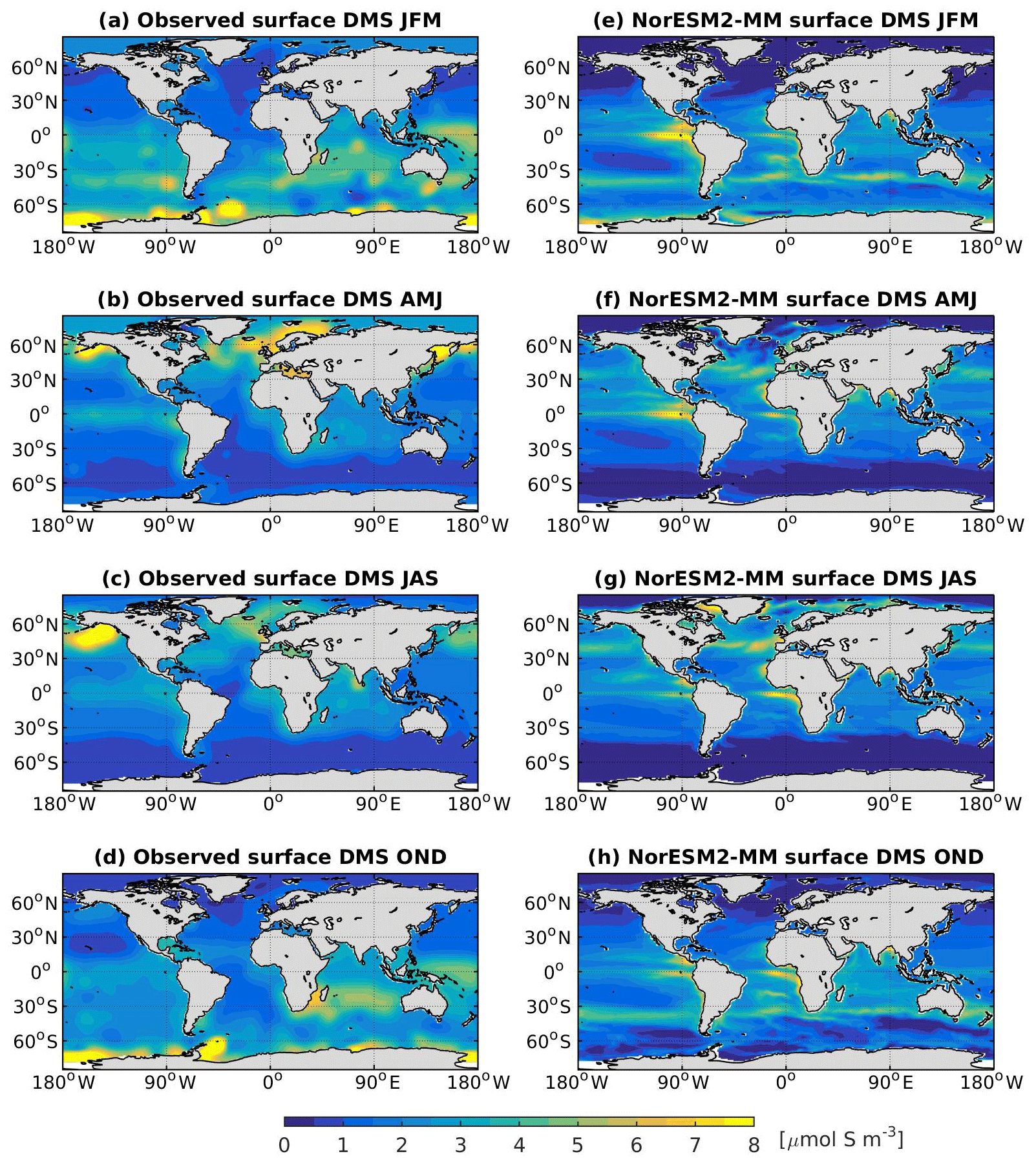
Figure 15Seasonally averaged surface concentration of DMS from observations (a–d) and as simulated in NorESM2-MM (e–h).
The simulated DMS concentration in the North Atlantic is comparable with observations. In the Southern Ocean, the model produces the observed high concentrations during summer months (JFM) along the 40–45∘ S latitude band well (Fig. 15e). In winter periods, the DMS concentration approaches zero in the model owing to the excessively low productivity, whilst the observations still indicate values of approximately 1 µmol S m−3. For the present-day period (1971–2000), the simulated global DMS flux is 19.76±0.19 Tg S yr−1, which is at the lower end of observation-based estimates (17.6–34.4 Tg S yr−1).
5.10 Dissolved inorganic carbon and alkalinity
Except for the polar Southern Ocean, the surface alkalinity concentrations in NorESM1 are approximately 100 µmol L−1 higher than the observational estimate. And since the spin-up was forced with constant pre-industrial atmospheric CO2 concentrations, the surface DIC concentration is adjusted (also anomalously high bias; Figs. 16g and 17g) to yield the “correct” surface pCO2. Consequently, biases in surface DIC and alkalinity compensate for one another to yield the approximately correct carbonate ion concentration (i.e. alkalinity minus DIC), seawater CO2 buffer capacity, and air–sea CO2 fluxes.
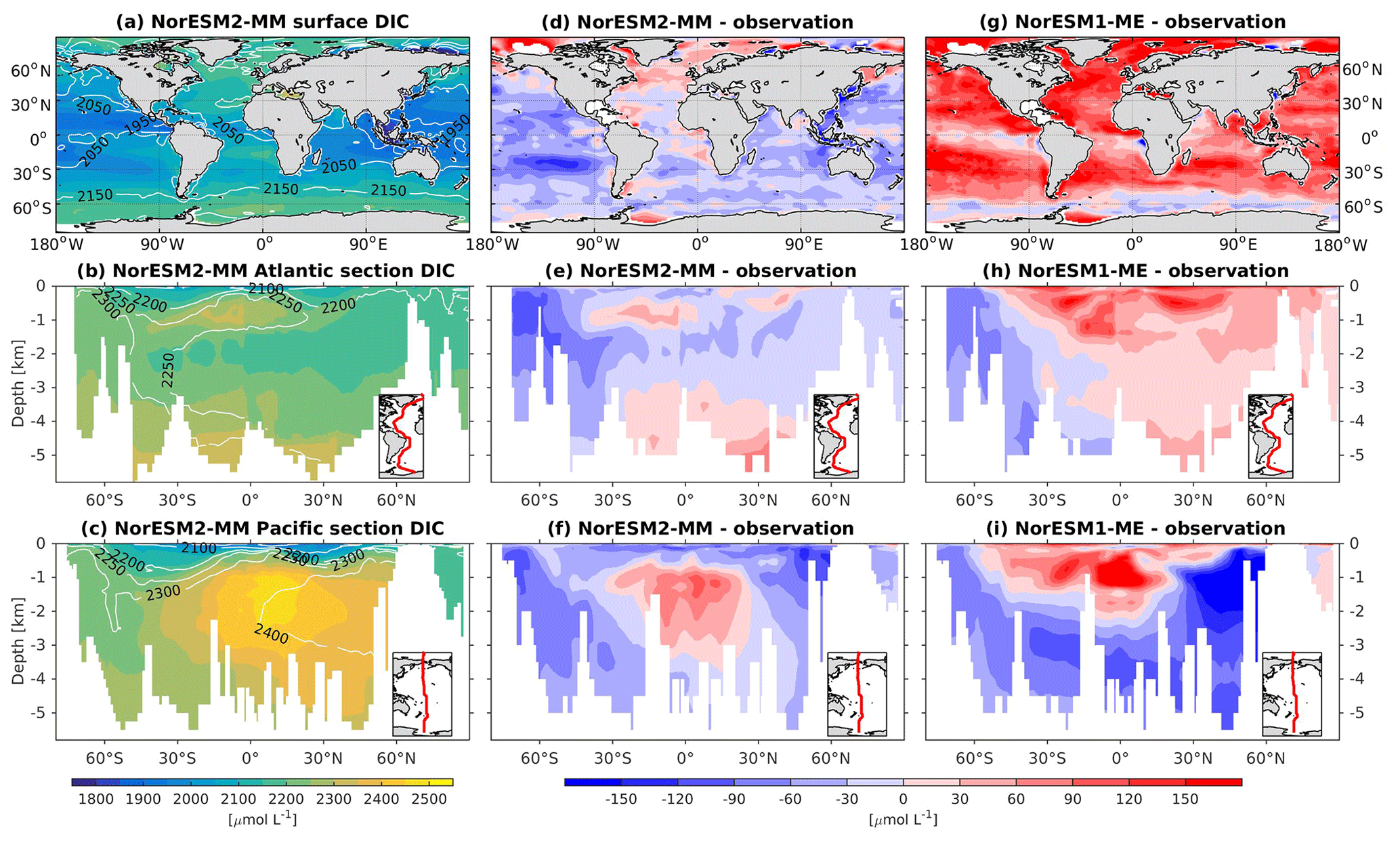
Figure 16Climatological dissolved inorganic carbon (DIC) values at the (a) surface and across the vertical sections of (b) the Atlantic and (c) Pacific in NorESM2-MM (colour shadings) and from observations (contour lines). Differences between NorESM2-MM (or NorESM1-ME) and observations are shown in panels (d)–(i).
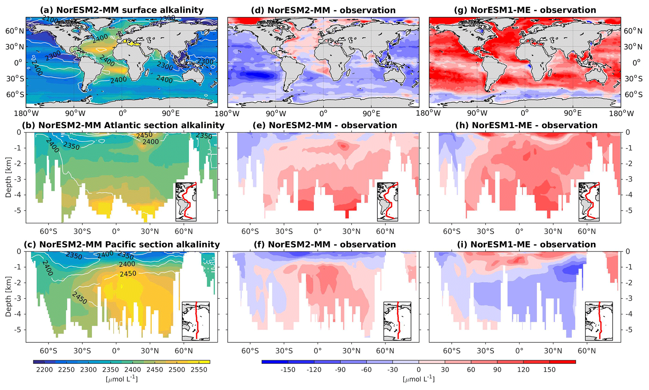
Figure 17Climatological alkalinity values at the (a) surface and across the vertical sections of (b) the Atlantic and (c) Pacific in NorESM2-MM (colour shadings) and from observations (contour lines). Differences between NorESM2-MM (or NorESM1-ME) and observations are shown in panels (d)–(i).
In NorESM2, we alleviate the surface alkalinity bias by increasing the surface sink associated with calcium carbonate production. This is done by increasing the CaCO3-to-phosphate uptake ratio ( in Table 1). As a result, the export of particulate CaCO3 increases from 0.49 Pg C yr−1 in NorESM1 to 0.66 Pg C yr−1, with both estimates still within the range of the observation-based synthesis of 0.52±0.15 Pg C yr−1 (Dunne et al., 2007). This modification increases the PIC:POC export ratio to 0.13 (0.06 in NorESM1; see also Table 3) and considerably improves the surface DIC and alkalinity concentrations in NorESM2 (Figs. 16a, d and 17a, d). At the same time, the spatial correlations with observations are also improved, as is the normalized RMSE (see Fig. 2a, b). We note that in a few regions, e.g. the subtropical South Pacific, the model still underestimates the observed DIC and alkalinity concentrations. We note that the PIC:POC ratio is still within the large range of other studies (0.03 to 0.25; Koeve, 2002; Sarmiento et al., 2002)
As at the surface, the spatial distributions and normalized bias of interior DIC and alkalinity in the NorESM2 improve considerably throughout the water column relative to NorESM1 (Fig. 2a, b). In both the interior Atlantic and Pacific basins, the spatial distribution and magnitude of DIC biases closely resemble that seen in the nutrients (e.g. phosphate; Figs. 16e, f, 7e, f) when multiplied by the constant stoichiometry in the model (). This suggests that the mechanisms driving the nutrient bias are also responsible for the bias in interior DIC. For instance, the positive anomaly in the equatorial Pacific between 1 and 3 km depths originates from too much biological remineralization in the model.
The simulated interior alkalinity concentrations in NorESM2 between 1 and 3 km depths are anomalously high, which can be partially attributed to excessively low interior remineralization in the Atlantic (see also AOU values Fig. 12c) or overly high CaCO3 export production (Table 3).
5.11 Surface pCO2 and sea–air CO2 fluxes
The NorESM2 pCO2 spatial correlation relative to the observations is improved in almost all seasons when compared to NorESM1, while the NRMSE is reduced for JFM and AMJ months (Fig. 2c, d). Within these months, improvements are mostly seen in the Southern Ocean, where surface mixing that is too strong in NorESM1 leads to anomalously high pCO2. The climatological mean of contemporary surface pCO2 in NorESM2 compares well with the observational compilations, as seen in Fig. 18a and e. Similar improvements are also seen in the CO2 fluxes, for which NorESM2 simulates the broad spatial patterns relatively well (Fig. 18c, g). NorESM2 also produces a moderately weaker annual mean carbon flux in the northern middle to high latitudes than NorESM1. Figure 18f and h show the zonally averaged monthly surface pCO2 and CO2 fluxes in NorESM2. Here, the model also agrees well with the observation-based estimates (Fig. 18b, d) in terms of amplitude and temporal variability, with a distinct seasonal cycle between 20 and 45∘ south–north. In the extratropical oceans (between 45 and 65∘ N and south of 60∘ S), the simulated winter (January–March and July–September in the Northern and Southern Hemisphere, respectively) pCO2 is considerably lower than that seen in the observations. Consequently, the simulated carbon fluxes in these regions are in the opposite direction of those seen in the observations (Fig. 18d, h).
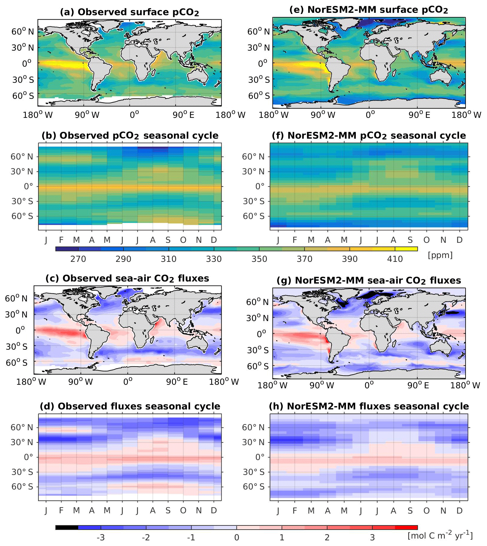
Figure 18Observed surface climatology maps of (a) the partial pressure of CO2 and (c) sea–air CO2 fluxes together with Hovmöller plots of the zonally averaged seasonal cycle of (b) surface pCO2 and (d) sea–air CO2 fluxes. Corresponding values from the NorESM2-MM simulation are shown in panels (e–g).
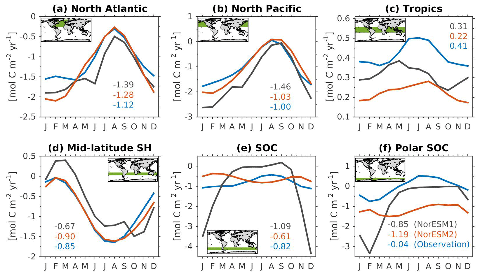
Figure 19Mean seasonal cycle of vertically integrated contemporary sea-to-air CO2 fluxes in the (a) North Atlantic (north of 20∘ N), (b) North Pacific (north of 20∘ N), (c) tropics (20∘ S–20∘ N), (d) mid-latitude Southern Hemisphere (20–40∘ S), (e) Southern Ocean (40–60∘ S), and (f) polar Southern Ocean (south of 60∘ S). Shown are values from NorESM1-ME (black), NorESM2-MM (red), and observational estimates (blue). Numbers within each panel depict the regional mean values averaged over all months.
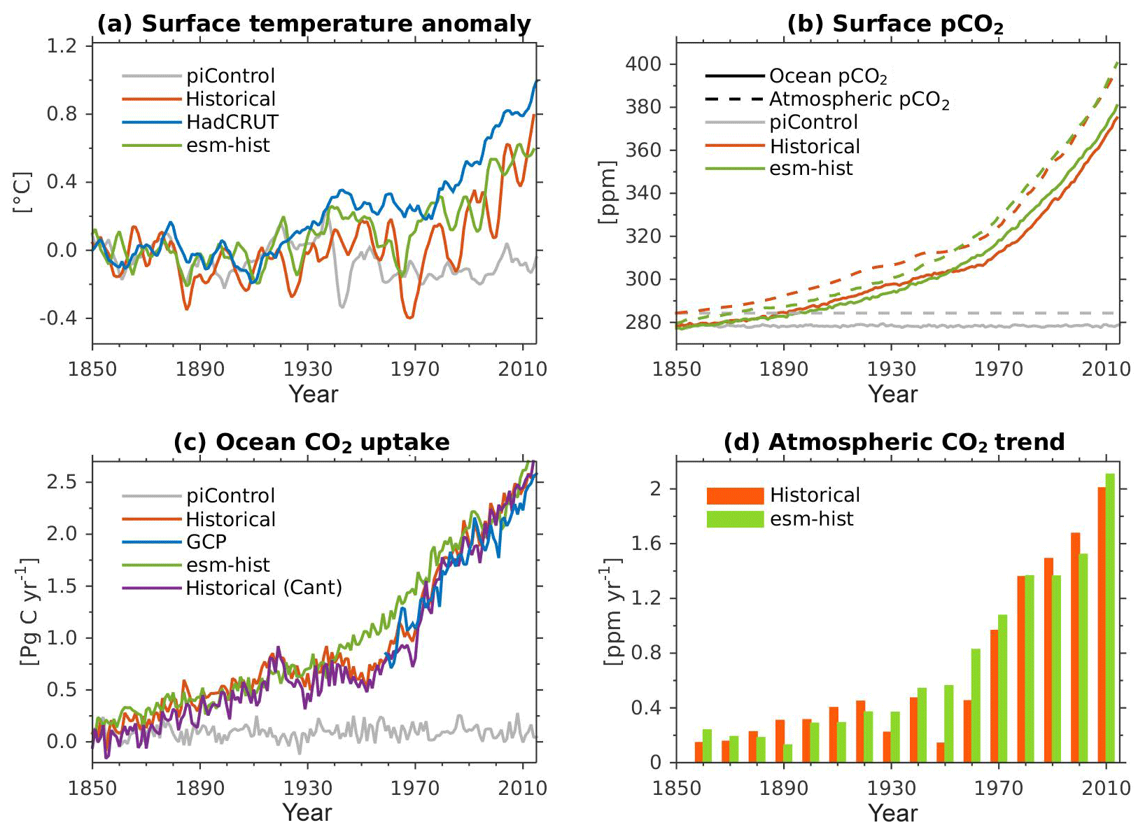
Figure 20Time series of global mean annual (a) surface air temperature anomalies relative to the 1850–1879 period, (b) surface ocean and atmospheric pCO2, (c) ocean CO2 uptake, and (d) atmospheric CO2 growth rate. Shown are values from the NorESM2-MM (grey) pre-industrial control and (orange) historical simulations. Green depicts results from the emissions-prescribed historical simulation with NorESM2-LM. The purple line in panel (c) represents the anthropogenic carbon uptake estimated by subtracting the natural carbon uptake from the total uptake (see also Sect. 3.2). Data for temperature and ocean carbon sinks (in blue) are estimates from HadCRUT4 and the Global Carbon Project (Morice et al., 2012; Le Quéré et al., 2018), respectively.
Figure 19 depicts the mean seasonal cycle of sea–air CO2 fluxes from NorESM models and observations, averaged over different regions. In the North Atlantic, North Pacific, and the mid-latitude Southern Hemisphere (between 20 and 40∘ S), the seasonal phase and mean integrated annual CO2 fluxes in NorESM2 compare better with the observations than those in NorESM1 (Fig. 19a, b, d). Nevertheless, NorESM2 simulates a stronger than observed carbon sink in the Labrador Sea and along the Kuroshio current extension during boreal winter months. We note that the Landschützer et al. (2014) data estimate higher surface pCO2 (hence a weaker carbon sink) in these regions than the observational estimates from Takahashi et al. (2009). Despite the warm SST bias in most of the tropics, NorESM2 simulates a moderately weaker than observed CO2 outgassing throughout the year (red line compared to blue line in Fig. 19c). A potential explanation for this is the weaker upwelling rates of DIC-rich deepwater masses in the model. In the Southern Ocean (south of 40∘ S), the strong bias in the seasonal amplitude in NorESM1 is considerably reduced (Fig. 19e, f) due to the improvements in the biological production in this region. Nevertheless, here the seasonal phase in NorESM2 is approximately reversed compared to observations: the strongest sink is simulated in the austral winter months, whereas observational estimates indicate summer months.
5.12 Transient changes
In this subsection, we describe the global mean surface air temperature and oceanic carbon uptake over the historical period (1850–2014) as simulated by NorESM2. For this, we discuss the two transient simulations: (i) historical and (ii) esm-hist. Similar to SST (see Fig. 3), there is a warm bias in the simulated surface air temperature. For the period of 1850–1859, the NorESM2 global mean surface air temperature is 14.5 ∘C compared to 13.7 ∘C from the HadCRUT4 dataset (Morice et al., 2012). Nevertheless, the simulated warming between 2005–2014 and 1850–1859 is 0.7 ∘C, comparable to that from observations of 0.8 ∘C (Fig. 20a). The warming in esm-hist is lower at 0.6 ∘C. Figure 20a also shows that NorESM2 (orange and green lines) simulates warming rates that are comparable to observations (blue line) between 1970 and 2010, but it shows a stronger cooling between 1950 and 1970 (historical and esm-hist).
In both simulations, the global mean surface ocean pCO2 follows the respective atmospheric CO2 trend over the simulation periods. Towards the end of the historical period, the oceanic pCO2 (solid green and orange lines) diverges from, i.e. is lower than, the atmospheric counterpart (dashed green and orange lines) by approximately 20 ppm (Fig. 20b). Consistent with the lower surface ocean (than the atmosphere) pCO2, the ocean carbon uptake continues to increase over most of the transient period in both simulations (Fig. 20c). In the historical simulation, the carbon sink stabilizes at roughly 0.7 Pg C yr−1 between 1910 and 1960. This flattening of the uptake strength is associated with the slowdown in the atmospheric CO2 growth rate. Figure 20d confirms that the atmospheric growth rate weakens during this time window (orange bars in Fig. 20d). In contrast, the carbon sink in esm-hist steadily increases during the same period, also consistent with the steady increase in the simulated prognostic atmospheric CO2 (green bars in Fig. 20d).
From 1960 onward, the atmospheric CO2 growth rates in both simulations increase almost linearly in time from 0.8 to more than 2.0 ppm yr−1. Consequently, the ocean carbon uptake strengths increase as well, from approximately 1 Pg C yr−1 in the 1960s up to roughly 2.5 Pg C yr−1 in 2014 (in both historical and esm-hist). Rapid strengthening of ocean carbon uptake is also evident in estimates from the Global Carbon Project (GCP, blue line in Fig. 20; Le Quéré et al., 2018). For the 1980s and 1990s, the simulated carbon uptake is also well within the IPCC (Intergovernmental Panel for Climate Change, Denman et al., 2007) estimates (Table 4). In NorESM2, a new tracer, DICnat, has been implemented (see also Sect. 3.2), and it enables us to more accurately estimate the anthropogenic carbon uptake and storage in the ocean. Using this tracer, we can also estimate the net flux of anthropogenic carbon into the ocean during the historical period, as depicted by the purple line in Fig. 20c. The strong resemblance between the orange and purple lines suggests that the long-term trend in oceanic carbon sinks is associated with the increasing atmospheric CO2 rather than changes in climate states (as expected for the historical runs in which the change in the climate state is relatively small). We note that, in the pre-industrial control simulation, the ocean is a weak net carbon sink of approximately 0.1 Pg C yr−1. Table 4 also shows that the cumulative carbon uptake by the ocean for 1850–1994 and 1994–2011 is well within the observation-based estimates. The cumulative carbon uptake in NorESM2 is lower than that of NorESM1 and compares better with observations.
(Denman et al., 2007)(Denman et al., 2007)(Gruber et al., 2019)(Gruber et al., 2019)Table 4Annual and accumulated ocean carbon uptakes simulated by NorESM1 and NorESM2 as well as from observation-based estimates.
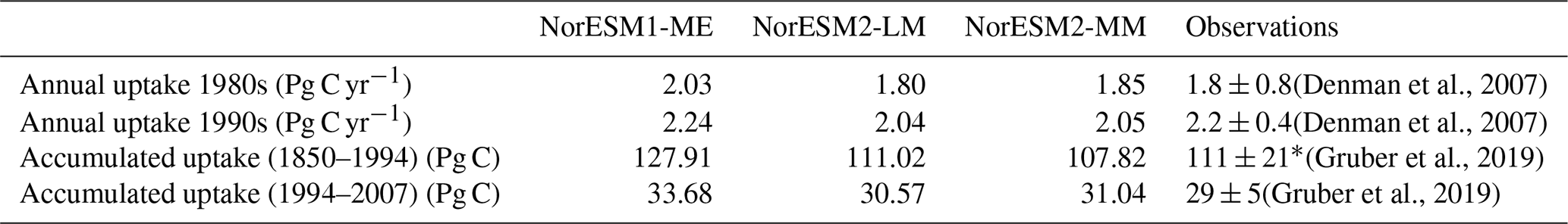
* 1800–1994.
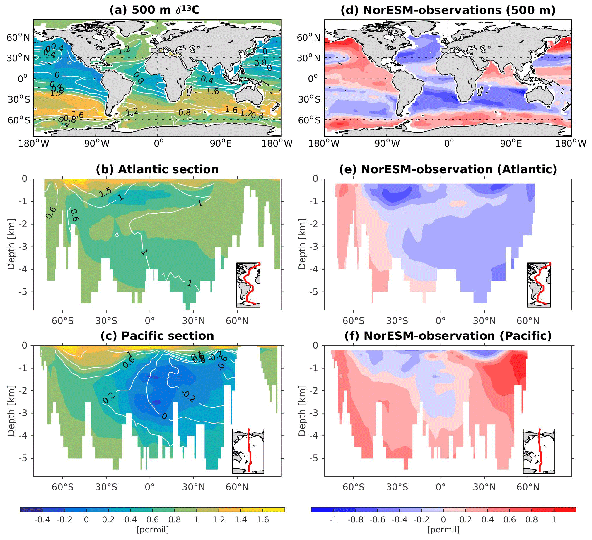
Figure 21Climatological δ13C values at (a) 500 m of depth and across the vertical sections of (b) the Atlantic and (c) Pacific from NorESM2-OC (colour shadings) and observations (contour lines). Differences between NorESM2-OC and observations are shown as colour shadings in panels (d)–(f).
5.13 Distribution of δ13C and Δ14C
As stated above, the carbon isotope tracers are not included in the coupled ESM configuration and only simulated in a pre-industrial stand-alone ocean configuration. We also note that although the stand-alone ocean simulation is not a direct representative of the coupled ESM simulation, its equilibrium ocean state is very comparable. For instance, the interior distributions of phosphate and DIC concentration in the stand-alone ocean simulation (Supplement Figs. S6, S7) share very similar characteristics with that produced in the coupled configuration (Figs. 7a–c, 16a–c). At the end of pre-industrial spin-up, Fig. 21a–c show that the spatial pattern of δ13C is in fair agreement with the gridded pre-industrial observational estimate of Eide et al. (2017). Nevertheless, the ocean component of NorESM2 simulates weaker variability than observed; i.e. it is unable to reproduce very low (negative) and high (positive) values. Therefore, the simulated δ13C concentrations in the relatively younger water masses, such as the North Atlantic Deep Water (NADW) and the Antarctic Intermediate Water (AAIW), have a negative bias relative to the observations (Fig. 21e). In contrast, positive biases are depicted in the older Antarctic Bottom Water (AABW) and in the deep North Pacific (Fig. 21e, f). The δ13C can be decomposed into biological and residual (air–sea gas exchange and circulation) components (Broecker and Maier-Reimer, 1992; Eide et al., 2017):
where δ13CBIO can be estimated as a function of phosphate and DIC distribution and their global mean values:
Applying this decomposition, we can attribute the majority of the differences between model and observational estimates of δ13C to biases in the biological component (Fig. 22). The δ13CBIO reveals that in the Southern Ocean (south of ∼55∘ S), as well as in its exported deep waters, NorESM2-OC simulates δ13C that is too high due to the excessively small regenerated signal in these waters. The negative δ13C anomaly in the North Atlantic of about −0.5 ‰ is the combination of a δ13CBIO signature that is too low in NADW (Fig. 22e) and an overly negative influence from air–sea gas exchange and circulation compared to observational estimates (the residual term δ13CAS). In the Pacific the positive anomaly from the Southern Ocean persists throughout most of the basin due to excessively weak remineralization, except at intermediate depths at which remineralization is high (see also AOU; Fig. 12).
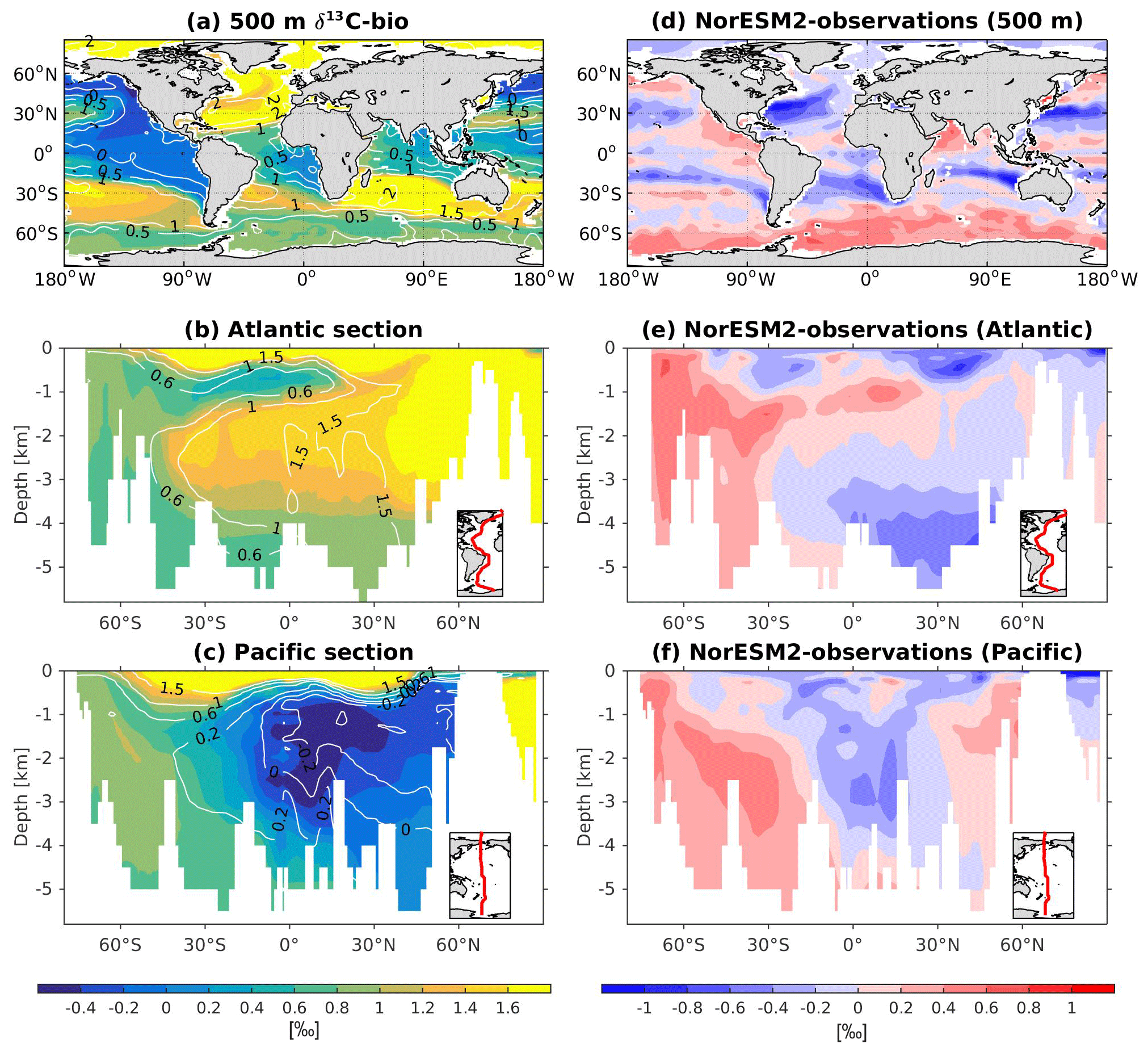
Figure 22Climatological fields of the biological component of δ13C (i.e. δ13CBIO) at (a) 500 m of depth and across the vertical sections of (b) the Atlantic and (c) Pacific from NorESM2-OC (colour shadings) and observations (contour lines). Differences between NorESM2-OC and observations are shown as colour shadings in panels (d)–(f).
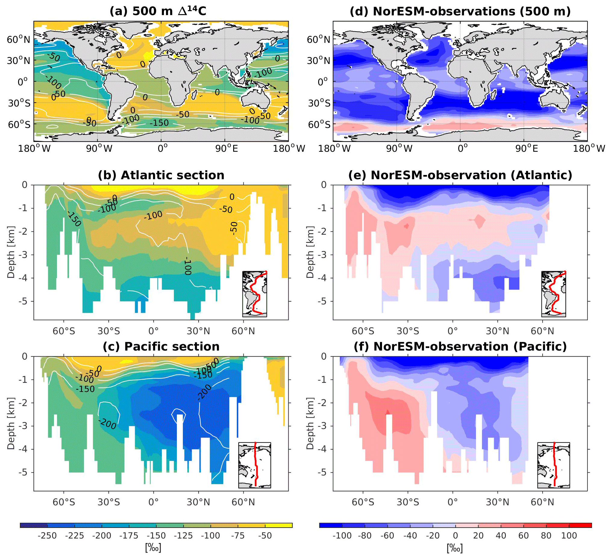
Figure 23Climatology Δ14C values at (a) 500 m of depth and across the vertical sections of (b) the Atlantic and (c) Pacific from NorESM2-OC (colour shadings) and observations (contour lines). Differences between NorESM2-OC and observations are shown as colour shadings in panels (d)–(f).
The simulated Δ14C distribution is in general agreement with the pre-industrial observational estimate by Key et al. (2004). Nevertheless, interior model–observation biases are in the range of ±50 ‰. Waters south of 60∘ S are positively biased compared to observations (Fig. 23), indicating waters in this region that are too young and well ventilated. This positive bias of 20 ‰–50 ‰ is carried into the Atlantic and Pacific basins (Fig. 23e–f) and is equivalent to an underestimation of radiocarbon age by 200–400 years. North of the Equator, a negative bias of similar magnitude indicates water masses that are too old in the Atlantic basin below 3 km of depth as well as throughout the water column in the northern half of the Pacific basin. The top 800 m of the water column has a negative bias of 100 ‰, which we attribute to the overly negative atmospheric p14CO2 before calibration (−36 ‰) and biases in air–sea equilibration and fractionation. Calibrated Δ14Catm is by definition 0 ‰, δ13Catm equilibrates at −7.5 ‰, and atmospheric pCO2 is 294 ppm at the end of the simulation.
The ocean biogeochemical component of the Norwegian Earth System Model (NorESM) has been updated from version 1 (as used in CMIP5) to version 2 (NorESM2). These developments focus on alleviating known biases in the mean states and seasonal cycles of key variables when compared to the observations. This paper describes new and improved processes, introduces newly implemented diagnostic and carbon isotope tracers, and highlights the model improvements relative to the earlier model version.
On the biogeochemistry side, we have introduced a revision to the particulate organic carbon vertical sinking scheme, an improved tuning of ecosystem parameters, riverine inputs of nutrients and other biogeochemical constituents, an updated air–sea gas exchange parameterization, and atmospheric deposition of nitrogen. In NorESM2, the ocean biogeochemistry also simulates (i) fully interactive oceanic DMS fluxes coupled to the atmospheric model, (ii) newly implemented preformed tracers, which enable us to perform a more detailed diagnosis of physical and biogeochemical sources and sinks in future studies, and (iii) carbon isotopes that can be used e.g. in extended paleo-timescale simulations.
On the physical side, the simulated Atlantic Meridional Overturning Circulation strength is considerably improved. An hourly coupling (previously daily) across the ocean–atmosphere–ice interfaces has been implemented. Intensive fully coupled testing prompted further attempts to optimize mixed layer physics parameters, which slightly reduce the bias in MLD when compared to our earlier model version.
In connection to our contribution to the CMIP6 simulations, two model configurations have been prepared, NorESM2-LM and NorESM2-MM, and the latter adopts a higher atmospheric resolution. In both versions, the ocean components are identical. Following the CMIP6 protocols (Eyring et al., 2016a), we have performed pre-industrial control (piControl, years 1850–2349) and transient climate (historical, years 1850–2014) simulations. Here, we analysed the simulations performed using both model versions.
As a result of the above developments, the overall performance of NorESM2 in simulating the climatological state of interior ocean biogeochemistry has improved considerably. Some of the key improvements include (i) better representation of the equatorial Pacific OMZ, (ii) improved interior nutrient distributions, and (iii) representation of iron limitation in the Southern Ocean, the equatorial Pacific, and North Pacific.
With respect to transient ocean carbon sinks, previous studies have indicated the importance of the background biogeochemical state, such as alkalinity, dissolved inorganic carbon, and buffer capacity, in order to adequately simulate the long-term trends (Hauck and Völker, 2015; Fassbender et al., 2018; Lebehot et al., 2019). NorESM1 exhibits a considerable bias for the background biogeochemical state, especially in surface alkalinity concentrations. These biases have been substantially reduced in NorESM2, resulting in a more adequate representation of the background buffer factor and improved model fidelity in simulating the temporal evolution of the ocean carbon sink.
The seasonality of upper-ocean biogeochemistry has been identified as critical for quantifying a model's uncertainty in its long-term projections of oceanic carbon uptake (Fassbender et al., 2018). Further, with ongoing anthropogenic CO2 emissions, the seasonal variability of regional sea–air CO2 fluxes is expected to amplify. This amplification, which is linear for the thermal component and non-linear for the biophysical component of oceanic pCO2 (Fassbender et al., 2018), can also impact the long-term evolution of sea–air CO2 fluxes. In this aspect, NorESM1 simulates a considerable bias in the seasonal cycle of biological production and air–sea CO2 fluxes, particularly in the Southern Ocean. The updated set of ecosystem parameters in NorESM2 is able to mitigate these biases to some extent. In the North Atlantic, North Pacific, and most parts of the Southern Ocean, the seasonal cycle (both in phase and amplitude) of primary production and CO2 fluxes in NorESM2 reflects observational estimates and their driving mechanisms more accurately (Landschützer et al., 2018). We note, however, that there is a mismatch between the CO2 flux seasonal cycle in observations and NorESM2 in the Southern Ocean between 40 and 60∘ N. Closer attention to the associated physical (e.g. solubility) and biogeochemical (e.g. biological productivity) drivers in this region is needed when considering future scenarios. However, general seasonal characteristics are improved, and we are confident that NorESM2 will provide a better estimate of future changes.
Despite numerous model improvements, several biases remain in the updated model. A long-standing issue of nutrient trapping in the intermediate depth of the equatorial Pacific persists. Here, the simulated phosphate concentration is still higher than observed, but the bias is less severe than that of NorESM1. Consistently, dissolved inorganic carbon is still anomalously high and oxygen too low in the same region. The simulated Southern Ocean still has ventilation that is too strong, leading to biases in the newly formed bottom water mass. Other physical biases, such as the Antarctic Bottom Water penetrating too far north, also contribute to the simulated model–data differences in the interior North Atlantic.
Currently, evaluations of ocean biogeochemical components in ESMs have been largely focused on assessing the model ability to simulate the mean climatological state. However, further options exist (Eyring et al., 2016b; Heinze et al., 2019). The ocean biogeochemical observing community has put a lot of effort into sustaining key monitoring networks, such as the Surface CO2 Atlas (SOCAT; Bakker et al., 2014) and the Global Ocean Data Analysis Project (GLODAP; Olsen et al., 2016). This critical observational network has provided additional valuable constraints for ESMs, such as by confronting model ability to simulate the seasonality of surface ocean pCO2 and long-term trends in surface ocean pCO2 (Tjiputra et al., 2014), ocean acidification (Lauvset et al., 2016), and deoxygenation (Tjiputra et al., 2018). As ESMs simulate emerging climate change signals in the coming decades (Henson et al., 2017), sustaining these observations into the future is becoming more important than ever.
In order to tackle the challenges associated with climate change, ocean modules in Earth system models could be further upgraded to include interactive methane (CH4), nitrous oxide (N2O), and biogenic volatile organic compound (BVOC) cycles for enabling model projections in respective emission-driven frameworks. Moreover, NorESM2 still has a relatively simple marine biology that would benefit from more key functional groups and their sensitivity to climatic stressors. In preparation for the anticipated increasing spatial resolution in the physical components of the model, different data assimilation methods (combined with state parameter estimation on the basis of observations) are currently being explored to enable us to perform optimizations of the current ecosystem parameterization more efficiently (Tjiputra et al., 2007; Gharamti et al., 2017).
Further NorESM internal improvements may consider online-estimated or prognostic particulate organic carbon emissions from the ocean biogeochemistry to the atmosphere. Currently, we use fixed particulate organic carbon emissions from the ocean linked to an upper-ocean chlorophyll a climatology. The spatial distribution and temporal characteristics of DMS emissions may have an impact on the strength of the feedback involving DMS and aerosol–cloud interactions. Dust and iron or phosphate contained therein as well as nitrogen deposition will be computed in the future version of the atmospheric NorESM module; this may provide more realistic nutrient input and thus lead to feedbacks in a coupled ESM. The biogeochemical exchange processes are also dependent on sea ice cover and require better knowledge of air–sea interaction processes in polar and subpolar regions. Mineralization processes in land regions may change under climate change conditions, leading to important changes in nutrient fluxes into the ocean biogeochemical systems. Biogenic volatile organic compounds (BVOCs) and halocarbons emitted from the ocean have been suspected to influence atmospheric chemistry e.g. in the stratosphere. It will certainly be the ambition of further developments to investigate the sensitivity of these processes to climate change to increase complexity where needed.
Beyond their current applications, future ESMs should be developed further to provide societally relevant information for policy decisions on climate mitigation and adaptation measures. This includes potential climate hazards to societies (such as marine heatwaves, sudden pH drops, and spreading low-oxygen zones in the oceans) and the risks emerging from the combination of hazards, vulnerabilities, and exposures (Oppenheimer et al., 2014). The future inclusion of socio-economic dynamics in ESMs and their feedback to climate through societally transformative action remains a big challenge (Giupponi et al., 2013), while a new ocean-related socio-economic scenario framework (OSPs) has been developed mirroring the established Shared Socioeconomic Pathways or SSPs (Maury et al., 2017). On the other hand, refining process complexity and increasing resolution may not be the only alternatives for further model development as the results of more complex model simulations become more difficult to interpret (Bony et al., 2011). Therefore, simplified models and ESMs of intermediate complexity, including the respective simplified ocean biogeochemistry modules, will need to be developed and used in parallel (for instance, Steinacher et al., 2013).
The NorESM2 codes, including the Bergen Layered Ocean Model and the isopycnic-based Hamburg Oceanic Carbon Cycle (BLOM-iHAMOCC), can be downloaded from https://doi.org/10.5281/zenodo.3760870 (Seland et al., 2020b).
The NorESM CMIP5 and CMIP6 model outputs can be accessed through the Earth System Grid Federation (ESGF) decentralized database (https://esgf-node.llnl.gov, last access: 9 December 2019, Bentsen et al., 2019).
All observational data used in this paper are publicly available, including the following: World Ocean Atlas (https://www.nodc.noaa.gov/OC5/woa13/, last access: 29 March 2019, Locarnini et al., 2013; Zweng et al., 2013; Garcia et al., 2013a, b), Global Ocean Data Analysis Project version 2 (https://www.glodap.info/, last access: 1 November 2019, Lauvset et al., 2016), surface mixed layer depth (http://www.ifremer.fr/cerweb/deboyer/mld/home.php, last access: 29 March 2019, de Boyer Montégut et al., 2004), surface pCO2 and air–sea CO2 fluxes (https://www.nodc.noaa.gov/ocads/oceans/SP_CO2_1982_2011_ETH_SOM_FFN.html, last access: 28 March 2019, Landschützer et al., 2015), ocean primary production (https://www.science.oregonstate.edu/ocean.productivity/, last access: 29 March 2019, Behrenfeld and Falkowski, 1997; Westberry et al., 2008), dimethyl sulfide (https://www.bodc.ac.uk/solas_integration/implementation_products/group1/dms/, last access: 1 September 2019, Lana et al., 2011), δ14C and CFC-11 (https://www.nodc.noaa.gov/ocads/oceans/glodap/, last access: 2 May 2019, Key et al., 2004), and δ13C (https://www.bcdc.no/data-products.html, last access: 1 November 2019, Eide et al., 2017).
The supplement related to this article is available online at: https://doi.org/10.5194/gmd-13-2393-2020-supplement.
JFT, JS, ALM, MB, CH, IB, and SG contributed to developing and implementing the iHAMOCC model code changes. JFT, JS, MB, ALM, AG, DO, and ØS designed, tested, and performed the experiments described in the paper. JFT, JS, ALM, and YH analysed the model simulations. All authors contributed to the writing of the paper.
The authors declare that they have no conflict of interest.
This article reflects only the authors' views – the funding agencies and their executive agencies are not responsible for any use that may be made of the information that the article contains.
The authors thank Joachim Segschneider and Julien Palmieri for their valuable and constructive feedback on the paper. We acknowledge support from the Bjerknes Centre for Climate Research. Ingo Bethke acknowledges support from the Trond Mohn Foundation (BFS2018TMT01). Anne L. Morée acknowledges PhD funding through the Faculty for Mathematics and Natural Sciences of the University of Bergen. High-performance computing and storage resources were provided by the Norwegian infrastructure for computational science (through projects nn2345k, nn2980k, nn1002k, nn9560k, ns2345k, ns2980k, ns1002k, and ns9560k). We also acknowledge Johan Liakka for providing technical assistance, Marco van Hulten for his help in licence development, and Jöran Maerz for the Teff-1 km data.
This research has been supported by the Norges Forskningsråd (grant nos. 229771, 270061, 295340, 275268, 295046) and the European Commission, Horizon 2020 Framework Programme (CRESCENDO, grant no. 641816).
This paper was edited by Paul Halloran and reviewed by Joachim Segschneider and Julien Palmieri.
Arora Vivek K., Boer, G. J., Friedlingstein, P., Eby, M., Jones, C., Christian, J., Bonan, G., Bopp, L., Brovkin, V., Cadule, P., Hajima, T., Ilyina, T., Lindsay, K., Tjiputra, J., and Wu., T.: Carbon Concentration and Carbon–Climate Feedbacks in CMIP5 Earth System Models, J. Climate, 26, 5289–5314, 2013. a
Assmann, K. M., Bentsen, M., Segschneider, J., and Heinze, C.: An isopycnic ocean carbon cycle model, Geosci. Model Dev., 3, 143–167, https://doi.org/10.5194/gmd-3-143-2010, 2010. a
Bakker, D. C. E., Pfeil, B., Smith, K., Hankin, S., Olsen, A., Alin, S. R., Cosca, C., Harasawa, S., Kozyr, A., Nojiri, Y., O'Brien, K. M., Schuster, U., Telszewski, M., Tilbrook, B., Wada, C., Akl, J., Barbero, L., Bates, N. R., Boutin, J., Bozec, Y., Cai, W.-J., Castle, R. D., Chavez, F. P., Chen, L., Chierici, M., Currie, K., de Baar, H. J. W., Evans, W., Feely, R. A., Fransson, A., Gao, Z., Hales, B., Hardman-Mountford, N. J., Hoppema, M., Huang, W.-J., Hunt, C. W., Huss, B., Ichikawa, T., Johannessen, T., Jones, E. M., Jones, S. D., Jutterström, S., Kitidis, V., Körtzinger, A., Landschützer, P., Lauvset, S. K., Lefèvre, N., Manke, A. B., Mathis, J. T., Merlivat, L., Metzl, N., Murata, A., Newberger, T., Omar, A. M., Ono, T., Park, G.-H., Paterson, K., Pierrot, D., Ríos, A. F., Sabine, C. L., Saito, S., Salisbury, J., Sarma, V. V. S. S., Schlitzer, R., Sieger, R., Skjelvan, I., Steinhoff, T., Sullivan, K. F., Sun, H., Sutton, A. J., Suzuki, T., Sweeney, C., Takahashi, T., Tjiputra, J., Tsurushima, N., van Heuven, S. M. A. C., Vandemark, D., Vlahos, P., Wallace, D. W. R., Wanninkhof, R., and Watson, A. J.: An update to the Surface Ocean CO2 Atlas (SOCAT version 2), Earth Syst. Sci. Data, 6, 69–90, https://doi.org/10.5194/essd-6-69-2014, 2014. a
Bauska, T. K., Baggenstos, D., Brook, E. J., Mix, A. C., Marcott, S. A., Petrenko, V. V., Schaefer, H., Severinghaus, J. P., and Lee, J. E.: Carbon isotopes characterize rapid changes in atmospheric carbon dioxide during the last deglaciation, P. Natl. Acad. Sci. USA, 113, 3465–3470, https://doi.org/10.1073/pnas.1513868113, 2016. a
Behrenfeld, M. and Falkowski, P.: Photosynthetic rates derived from satellite-based chlorophyll concentration, Limnol. Oceanogr., 42, 1–20, 1997. a, b
Bentsen, M., Bethke, I., Debernard, J. B., Iversen, T., Kirkevåg, A., Seland, Ø., Drange, H., Roelandt, C., Seierstad, I. A., Hoose, C., and Kristjánsson, J. E.: The Norwegian Earth System Model, NorESM1-M – Part 1: Description and basic evaluation of the physical climate, Geosci. Model Dev., 6, 687–720, https://doi.org/10.5194/gmd-6-687-2013, 2013. a, b
Bentsen, M., Oliviè, D. J. L., Seland, Ø., Toniazzo, T., Gjermundsen, A., Graff, L. S., Debernard, J. B., Gupta, A. K., He, Y., Kirkevåg, A., Schwinger, J., Tjiputra, J., Aas, K. S., Bethke, I., Fan, Y., Griesfeller, J., Grini, A., Guo, C., Ilicak, M., Karset, I. H. H., Landgren, O. A., Liakka, J., Moseid, K. O., Nummelin, A., Spensberger, C., Tang, H., Zhang, Z., Heinze, C., Iversen, T., and Schulz, M.: NCC NorESM2-MM model output prepared for CMIP6 CMIP historical, Earth System Grid Federation, https://doi.org/10.22033/ESGF/CMIP6.8040, 2019. a
Bentsen, M., Ilıcak, M., Nummelin, A., Guo, C., and Debernard, J. B.: Bergen Layered Ocean Model (BLOM): Description and evaluation of global ocean–sea-ice experiments, in preparation, 2020. a, b
Bernard, C. Y., Dürr, H. H., Heinze, C., Segschneider, J., and Maier-Reimer, E.: Contribution of riverine nutrients to the silicon biogeochemistry of the global ocean – a model study, Biogeosciences, 8, 551–564, https://doi.org/10.5194/bg-8-551-2011, 2011. a, b, c, d, e
Bernardello, R., Marinov, I., Palter, J. B., Sarmiento, J. L., Galbraith, E. D., and Slater, R. D.: Response of the ocean natural carbon storage to projected twenty-first-century climate change, J. Climate, 27, 2033–2053, https://doi.org/10.1175/JCLI-D-13-00343.1, 2014. a, b, c
Bony, S., Stevens, B., Held, I., Mitchell, J., Dufresne, J. L., Emanuel, K., Friedlingstein, P., Griffies, S., and Senior, S.: Carbon Dioxide and Climate: Perspectives on a Scientific Assessment, Position paper prepared for the WCRP Open Science Conference, Denver, USA, 24–28 October, 21 pp., 2011. a
Bopp, L., Resplandy, L., Orr, J. C., Doney, S. C., Dunne, J. P., Gehlen, M., Halloran, P., Heinze, C., Ilyina, T., Séférian, R., Tjiputra, J., and Vichi, M.: Multiple stressors of ocean ecosystems in the 21st century: projections with CMIP5 models, Biogeosciences, 10, 6225–6245, https://doi.org/10.5194/bg-10-6225-2013, 2013. a, b
Boyd, P. W. and Ellwood, M. J.: The biogeochemical cycle of iron in the ocean, Nat. Geosci., 3, 675–682, 2010. a
Braconnot, P., Harrison, S. P., Kageyama, M., Bartlein, P. J., Masson-Delmotte, V., Abe-Ouchi, A., Otto-Bliesner, B., and Zhao, Y.: Evaluation of climate models using paleoclimatic data, Nat. Clim. Change, 2, 417–424, https://doi.org/10.1038/nclimate1456, 2012. a
Breitbarth, E., Oschlies, A., and LaRoche, J.: Physiological constraints on the global distribution of Trichodesmium – effect of temperature on diazotrophy, Biogeosciences, 4, 53–61, https://doi.org/10.5194/bg-4-53-2007, 2007. a
Bretherton, F. P.: Earth System Science and Remote-Sensing, P. IEEE, 73, 1118–1133, https://doi.org/10.1109/Proc.1985.13242, 1985. a
Broecker, W. S.: “NO” a conservative water-mass tracer, Earth Planet. Sc. Lett., 23, 100–107, https://doi.org/10.1016/0012-821X(74)90036-3, 1974. a
Broecker W, S. and Peng, T. H.: Gas exchange rates between air and sea, Tellus, 26, 21–35, https://doi.org/10.1111/j.2153-3490.1974.tb01948.x, 1974. a
Broecker, W. S., and Maier-Reimer E.: The influence of air and sea exchange on the carbon isotope distribution in the sea, Global Biogeochem. Cy., 6, 315–320, https://doi.org/10.1029/92GB01672, 1992. a
Broecker, W. S. and McGee, D.: The 13C record for atmospheric CO2: What is it trying to tell us?, Earth Planet. Sc. Lett., 368, 175–182, https://doi.org/10.1016/j.epsl.2013.02.029, 2013. a
Bruland, K. W., Middag, R., and Lohan, M. C.: 8.2 – Controls of Trace Metals in Seawater, in: Treatise on Geochemistry (Second Edition), edited by: Holland, H. D. and Turekian, K. K., Elsevier, Oxford, 19–51, 2014. a
Bullister, J.: Updated (2014) Atmospheric CFC-11, CFC-12, CFC-113, CCl4 and SF6 Histories, available at: http://cdiac.ornl.gov/ftp/oceans/CFC_ATM_Hist/CFC_ATM_Hist_2014, last access: 5 December 2014. a
Bullister, J. L., Wisegarver, D. P., and Menzia, F. A.: The solubility of sulfur hexafluoride in water and seawater, Deep-Sea Res. Pt. I, 49, 175–187, 2002. a
Cabré, A., Marinov, I., Bernardello, R., and Bianchi, D.: Oxygen minimum zones in the tropical Pacific across CMIP5 models: mean state differences and climate change trends, Biogeosciences, 12, 5429–5454, https://doi.org/10.5194/bg-12-5429-2015, 2015. a, b
Chester, R.: Marine Geochemistry, 1st Edn., 702 pp., Springer, Netherlands, 1990. a
Crucifix, M.: Distribution of carbon isotopes in the glacial ocean: A model study, Paleoceanography, 20, PA4020, https://doi.org/10.1029/2005PA001131, 2005. a
Cubasch, U., Wuebbles, D., Chen, D., Facchini, M. C., Frame, D., Mahowald, N., and Winther, J.-G.: Introduction, in: Climate Change 2013: The Physical Science Basis, Contribution of Working Group I to the Fifth Assessment Report of the Intergovernmental Panel on Climate Change, edited by: Stocker, T. F., Qin, D., Plattner, G.-K., Tignor, M., Allen, S. K., Boschung, J., Nauels, A., Xia, Y., Bex, V. and Midgley, P. M., Cambridge University Press, Cambridge, United Kingdom and New York, NY, USA, 2013. a
Curry, W. B. and Oppo, D. W.: Glacial water mass geometry and the distribution of δ13C of ΣCO2 in the western Atlantic Ocean, Paleoceanography, 20, PA1017, https://doi.org/10.1029/2004PA001021, 2005. a
de Baar, H. J. W., de Jong, J. T. M., Bakker, D. C. E., Löscher, B. M., Veth, C., Bathmann, U., and Smetacek, V.: Importance of iron for phytoplankton spring blooms and CO2 drawdown in the Southern Ocean, Nature, 373, 412–415, 1995. a
de Boyer Montégut, C., Madec, G., Fischer, A. S., Lazar, A., and Iudicone, D.: Mixed layer depth over the global ocean: an examination of profile data and a profile-based climatology, J. Geophys. Res., 109, 12003, https://doi.org/10.1029/2004JC002378, 2004. a, b, c
Denman, K. L., Brasseur, G., Chidthaisong, A., Ciais, P., Cox, P. M., Dickinson, R. E., Hauglustaine, D., Heinze, C., Holland, E., Jacob, D., Lohmann, U., Ramachandran, S., da Silva Dias, P. L., Wofsy, S. C., and Zhang, X.: Couplings Between Changes in the Climate System and Biogeochemistry, in: Climate Change 2007: The Physical Science Basis, Contribution of Working Group I to the Fourth Assessment Report of the Intergovernmental Panel on Climate Change, edited by: Solomon, S., Qin, D., Manning, M., Chen, Z., Marquis, M., Averyt, K. B., Tignor, M., and Miller, H. L., Cambridge University Press, Cambridge, United Kingdom and New York, NY, USA, 2007. a, b, c
Dunne, J. P., Sarmiento, J. L., and Gnanadesikan, A.: A synthesis of global particle export from the surface ocean and cycling through the ocean interior and on the seafloor, Global Biogeochem. Cy., 21, GB4006, https://doi.org/10.1029/2006GB002907, 2007. a
Duteil, O., Koeve, W., Oschlies, A., Aumont, O., Bianchi, D., Bopp, L., Galbraith, E., Matear, R., Moore, J. K., Sarmiento, J. L., and Segschneider, J.: Preformed and regenerated phosphate in ocean general circulation models: can right total concentrations be wrong?, Biogeosciences, 9, 1797–1807, https://doi.org/10.5194/bg-9-1797-2012, 2012. a
Eide, M., Olsen, A., Ninnemann, U. S., and Johannessen, T.: A global ocean climatology of preindustrial and modern ocean δ13C, Global Biogeochem. Cy., 31, 515–534, https://doi.org/10.1002/2016GB005473, 2017. a, b, c, d, e, f
Eggleston, S. and Galbraith, E. D.: The devil's in the disequilibrium: multi-component analysis of dissolved carbon and oxygen changes under a broad range of forcings in a general circulation model, Biogeosciences, 15, 3761–3777, https://doi.org/10.5194/bg-15-3761-2018, 2018. a
Eyring, V., Bony, S., Meehl, G. A., Senior, C. A., Stevens, B., Stouffer, R. J., and Taylor, K. E.: Overview of the Coupled Model Intercomparison Project Phase 6 (CMIP6) experimental design and organization, Geosci. Model Dev., 9, 1937–1958, https://doi.org/10.5194/gmd-9-1937-2016, 2016a. a, b, c
Eyring, V., Gleckler, P. J., Heinze, C., Stouffer, R. J., Taylor, K. E., Balaji, V., Guilyardi, E., Joussaume, S., Kindermann, S., Lawrence, B. N., Meehl, G. A., Righi, M., and Williams, D. N.: Towards improved and more routine Earth system model evaluation in CMIP, Earth Syst. Dynam., 7, 813–830, https://doi.org/10.5194/esd-7-813-2016, 2016b. a
Fassbender, A. J., Rodgers, K. B., Palevsky, H. I., and Sabine, C. L.: Seasonal asymmetry in the evolution of surface ocean pCO2 and pH thermodynamic drivers and the influence on sea-air CO2 flux, Global Biogeochem. Cy., 32, 1476–1497, https://doi.org/10.1029/2017GB005855, 2018. a, b, c
Flato, G., Marotzke, J., Abiodun, B., Braconnot, P., Chou, S. C., Collins, W., Cox, P., Driouech, F., Emori, S., Eyring, V., Forest, C., Gleckler, P., Guilyardi, E., Jakob, C., Kattsov, V., Reason, C. and Rummukainen, M.: Evaluation of climate models, in: Climate Change 2013: The Physical Science Basis, Contribution of Working Group I to the IPCC AR5, Cambridge Univ. Press, Cambridge, UK, and New York, 741–882, 2013. a
Fox-Kemper, B., Ferrari, R., and Hallberg, R.: Parameterization of Mixed Layer Eddies. Part I: Theory and Diagnosis, J. Phys. Oceanogr., 38, 1145–1165, 2008. a
Friedlingstein, P., Cox, P., Betts, R., Bopp, L., et al.: Climate-carbon cycle feedback analysis: Results from the C4MIP model intercomparison, J. Climate, 19, 3337–3353, 2006. a
Gao, S., Schwinger, J., Bethke, I., Tjiputra, J., Hartmann, J., Mayorga, E., and Heinze, C.: Impact of riverine nutrients and carbon on future projections of marine biogeochemistry, in preparation, 2020. a
Garcia, H. E. and Gordon, L. I.: Oxygen solubility in seawater: Better fitting equations, Limnol. Oceanogr., 37, 1307–1312, 1992. a
Garcia H. E., Boyer, T. P., Locarnini, R. A., Mishonov, A. V., Antonov, J. I., Baranova, O. K., Zweng, M. M., Reagan, J. R., and Johnson, D. R.: World Ocean Atlas 2013, Volume 3: Dissolve Oxygen, Apparent Oxygen Utilization, and Oxygen Saturation, edited by: Levitus, S. and Mishonov, A., NOAA Atlas NESDIS 75, 29 pp., 2013a. a, b
Garcia H. E., Boyer, T. P., Locarnini, R. A., Mishonov, A. V:, Antonov, J. I., Baranova, O. K., Zweng, M. M., Reagan, J. R., and Johnson, D. R.: World Ocean Atlas 2013, Volume 4: Dissolved Inorganic Nutrients (phosphate, nitrate, silicate), edited by: Levitus, S. and Mishonov, A., NOAA Atlas NESDIS 76, 2013b. a, b, c, d
Gehlen, M., Séférian, R., Jones, D. O. B., Roy, T., Roth, R., Barry, J., Bopp, L., Doney, S. C., Dunne, J. P., Heinze, C., Joos, F., Orr, J. C., Resplandy, L., Segschneider, J., and Tjiputra, J.: Projected pH reductions by 2100 might put deep North Atlantic biodiversity at risk, Biogeosciences, 11, 6955–6967, https://doi.org/10.5194/bg-11-6955-2014, 2014. a, b
Gent, P. R. and McWilliams, J. C.: Isopycnal mixing in ocean circulation models, J. Phys. Oceanogr., 20, 150–155, 1990. a
Gharamti, M. E., Tjiputra, J., Bethke, I., Samuelsen, A., Skjelvan, I., Bentsen, M., and Bertino, L.: Ensemble data assimilation for ocean biogeochemical state and parameter estimation at different sites, Ocean Model., 112, 65–89, https://doi.org/10.1016/j.ocemod.2017.02.006, 2017. a
Giupponi, C., Borsuk, M. E:, de Vries, B. J. M., and Hasselmann, K.: Innovative approaches to integrated global change modelling, Environ. Modell. Softw., 44, 1–9, https://doi.org/10.1016/j.envsoft.2013.01.013, 2013. a
Goris, N., Tjiputra, J. F., Olsen, A., Schwinger, J., Lauvset, S. K., and Jeansson, E.: Constraining Projection-Based Estimates of the Future North Atlantic Carbon Uptake, J. Climate, 31, 3959–3978, https://doi.org/10.1175/JCLI-D-17-0564.1, 2018. a
Grossman, E. L. and Ku, T.-L.: Oxygen and carbon isotope fractionation in biogenic aragonite: temperature effects, Chem. Geol., 59, 59–74, 1986. a, b
Gruber, N. and Keeling, C. D.: An improved estimate of the isotopic air-sea disequilibrium of CO2: Implications for the oceanic uptake of anthropogenic CO2, Geophys. Res. Lett., 28, 555–558, https://doi.org/10.1029/2000GL011853, 2001. a
Gruber, N., Clement, D., Carter, B. R., Feely, R. A., van Heuven, S., Hoppema, M., Ishii, M., Key, R. M., Kozyr, A., Lauvset, S. K., Lo Monaco, C., Mathis, J. T., Murata, A., Olsen, A., Perez, F. F., Sabine, C. L., Tanhua, T., and Wanninkhof, R.: The oceanic sink for anthropogenic CO2 from 1994 to 2007, Science, 363, 1193–1199, https://doi.org/10.1126/science.aau5153, 2019. a, b
Guo, C., Bentsen, M., Bethke, I., Ilicak, M., Tjiputra, J., Toniazzo, T., Schwinger, J., and Otterå, O. H.: Description and evaluation of NorESM1-F: a fast version of the Norwegian Earth System Model (NorESM), Geosci. Model Dev., 12, 343–362, https://doi.org/10.5194/gmd-12-343-2019, 2019. a, b
Hartmann, J.: Bicarbonate-fluxes and CO2-consumption by chemical weathering on the Japanese Archipelago – Application of a multi-lithological model framework, Chem. Geol., 265, 237–271, 2009. a
Hauck, J. and Völker, C.: Rising atmospheric CO2 leads to large impact of biology on Southern Ocean CO2 uptake via changes of the Revelle factor, Geophys. Res. Lett., 42, 1459–1464, https://doi.org/10.1002/2015GL063070, 2015. a
Henson, S. A., Beaulieu, C., Ilyina, T., John, J. G., Long, M., Séférian, R., Tjiputra, J., and Sarmiento, J. L.: Rapid emergence of climate change in environmental drivers of marine ecosystem, Nat. Commun., 8, 14682, https://doi.org/10.1038/ncomms14682, 2017. a
Heinze, C., Eyring, V., Friedlingstein, P., Jones, C., Balkanski, Y., Collins, W., Fichefet, T., Gao, S., Hall, A., Ivanova, D., Knorr, W., Knutti, R., Löw, A., Ponater, M., Schultz, M. G., Schulz, M., Siebesma, P., Teixeira, J., Tselioudis, G., and Vancoppenolle, M.: ESD Reviews: Climate feedbacks in the Earth system and prospects for their evaluation, Earth Syst. Dynam., 10, 379–452, https://doi.org/10.5194/esd-10-379-2019, 2019. a, b
Holden, P. B., Edwards, N. R., Müller, S. A., Oliver, K. I. C., Death, R. M., and Ridgwell, A.: Controls on the spatial distribution of oceanic δ13CDIC, Biogeosciences, 10, 1815–1833, https://doi.org/10.5194/bg-10-1815-2013, 2013. a
Hoogakker, B. A. A., Elderfield, H., Schmiedl, G., McCave, I. N., and Rickaby, R. E. M.: Glacial-interglacial changes in bottom-water oxygen content on the Portuguese margin, Nat. Geosci., 8, 40–43, https://doi.org/10.1038/ngeo2317, 2015. a
Ilyina, T., Six, K. D., Segschneider, J., Maier-Reimer, E., Li, H., and Núñez Riboni, I.: Global ocean biogeochemistry model HAMOCC: model architecture and performance as component of the MPI-Earth System Model in different CMIP5 experimental realizations, J. Adv. Model. Earth Sy., 5, 287–315, https://doi.org/10.1029/2012MS000178, 2013. a
Ito, T., Follows, M. J., and Boyle, E. A.: Is AOU a good measure of respiration in the oceans?, Geophys. Res. Lett., 31, L17305, https://doi.org/10.1029/2004GL020900, 2004. a
Jahn, A., Lindsay, K., Giraud, X., Gruber, N., Otto-Bliesner, B. L., Liu, Z., and Brady, E. C.: Carbon isotopes in the ocean model of the Community Earth System Model (CESM1), Geosci. Model Dev., 8, 2419–2434, https://doi.org/10.5194/gmd-8-2419-2015, 2015. a
Jochum, M., Briegleb, B. P., Danabasoglu, G., Large, W. G., Norton, N. J., Jayne, S. R., Alford, M. H., and Bryan, F. O.: The Impact of Oceanic Near-Inertial Waves on Climate, J. Climate, 26, 2833–2844, https://doi.org/10.1175/JCLI-D-12-00181.1, 2013. a
Jones, C. D., Arora, V., Friedlingstein, P., Bopp, L., Brovkin, V., Dunne, J., Graven, H., Hoffman, F., Ilyina, T., John, J. G., Jung, M., Kawamiya, M., Koven, C., Pongratz, J., Raddatz, T., Randerson, J. T., and Zaehle, S.: C4MIP – The Coupled Climate–Carbon Cycle Model Intercomparison Project: experimental protocol for CMIP6, Geosci. Model Dev., 9, 2853–2880, https://doi.org/10.5194/gmd-9-2853-2016, 2016. a
Keller, K. and Morel, F. M. M.: A model of carbon isotopic fractionation and active carbon uptake in phytoplankton, Mar. Ecol. Prog. Ser., 182, 295–298, https://doi.org/10.3354/meps182295, 1999. a
Keller, M., Bellows, W., and Guillard, R.: Dimethyl sulfide production in marine phytoplankton, in: Biogenic sulfur in the environment, edited by: Saltzman, E. and Cooper, W., ACS-Symposium series, New Orleans, Louisiana, American Chemical Society, 167–181, 1989. a
Kessler, A. and Tjiputra, J.: The Southern Ocean as a constraint to reduce uncertainty in future ocean carbon sinks, Earth Syst. Dynam., 7, 295–312, https://doi.org/10.5194/esd-7-295-2016, 2016. a
Kessler, A., Galaasen, E. V., Ninnemann, U. S., and Tjiputra, J.: Ocean carbon inventory under warmer climate conditions – the case of the Last Interglacial, Clim. Past, 14, 1961–1976, https://doi.org/10.5194/cp-14-1961-2018, 2018. a
Key, R. M., Kozyr, A., Sabine, C. L., Lee, K., Wanninkhof, R., Bullister, J. L., Feely, R. A., Millero, F. J., Mordy, C., and Peng, T. H.: A global ocean carbon climatology: Results from Global Data Analysis Project (GLODAP), Global Biogeochem. Cy., 18, GB4031, https://doi.org/10.1029/2004GB002247, 2004. a, b, c, d, e, f
Kloster, S., Feichter, J., Maier-Reimer, E., Six, K. D., Stier, P., and Wetzel, P.: DMS cycle in the marine ocean-atmosphere system – a global model study, Biogeosciences, 3, 29–51, https://doi.org/10.5194/bg-3-29-2006, 2006. a
Koeve, W.: Upper ocean carbon fluxes in the Atlantic Ocean: The importance of the POC:PIC ratio, Global Biogeochem. Cy., 1, 1056, https://doi.org/10.1029/2001GB001836, 2002. a
Kriest, I.: Different parameterizations of marine snow in a 1-D model and their influence on representation of marine snow, nitrogen budget and sedimentation, Deep-Sea Res. Pt. I, 49, 2133–2162, 2002. a
Kriest, I. and Evans, G.: Representing phytoplankton aggregates in biogeochemical models, Deep-Sea Res. Pt. I, 46, 1841–1859, 1999. a
Kriest, I. and Oschlies, A.: On the treatment of particulate organic matter sinking in large-scale models of marine biogeochemical cycles, Biogeosciences, 5, 55–72, https://doi.org/10.5194/bg-5-55-2008, 2008. a
Kriest, I. and Oschlies, A.: MOPS-1.0: towards a model for the regulation of the global oceanic nitrogen budget by marine biogeochemical processes, Geosci. Model Dev., 8, 2929–2957, https://doi.org/10.5194/gmd-8-2929-2015, 2015. a
Kwiatkowski, L., Bopp, L., Aumont, O., Ciais, P., Cox, P. M., Laufkötter, C., Li, Y., and Séférian, R.: Emergent constraints on projections of declining primary production in the tropical oceans, Nat. Clim. Change, 7, 355–359, https://doi.org/10.1038/NCLIMATE3265, 2017. a
Lana, A., Bell, T. G., Simó, R., Vallina, S. M., Ballabrera-Poy, J., Kettle, A. J., Dachs, J., Bopp, L., Saltzman, E. S., Stefels, J., Johnson, J. E., and Liss, P. S.: An updated climatology of surface dimethlysulfide concentrations and emission fluxes in the global ocean, Global Biogeochem. Cy., 25, GB1004, https://doi.org/10.1029/2010GB003850, 2011. a, b, c
Landschützer, P., Gruber, N., Bakker, D., and Schuster, U.: Recent variability of the global ocean carbon sink, Global Biogeochem. Cy., 28, 927–949, https://doi.org/10.1002/2014GB004853, 2014. a
Landschützer, P., Gruber, N., and Bakker, D. C. E.: A 30 years observation-based global monthly gridded sea surface pCO2 product from 1982 through 2011 (NCEI Accession 0160558), Version 2.2. NOAA National Centers for Environmental Information, Dataset, https://doi.org/10.3334/cdiac/otg.spco2_1982_2011_eth_somffn, 2015. a, b, c
Landschützer, P., Gruber, N., Bakker, D. C. E., Stemmler, I., and Six, K. D.: Strengthening seasonal marine CO2 variations due to increasing atmospheric CO2, Nat. Clim. Change, 8, 146–150, https://doi.org/10.1038/s41558-017-0057-x, 2018. a
Large, W. and Yeager, S.: Diurnal to Decadal Global Forcing for Ocean and Sea-Ice Models: The Data Sets and Flux Climatologies, Tech. Note NCAR/TN-460+STR, National Center of Atmospheric Research, Boulder, Colorado, USA, 2004. a
Lauvset, S. K., Key, R. M., Olsen, A., van Heuven, S., Velo, A., Lin, X., Schirnick, C., Kozyr, A., Tanhua, T., Hoppema, M., Jutterström, S., Steinfeldt, R., Jeansson, E., Ishii, M., Perez, F. F., Suzuki, T., and Watelet, S.: A new global interior ocean mapped climatology: the 1° × 1° GLODAP version 2, Earth Syst. Sci. Data, 8, 325–340, https://doi.org/10.5194/essd-8-325-2016, 2016. a, b, c, d
Laws, E. A., Popp, B. N., Bidigare, R. R., Kennicutt, M. C., and Macko, S. A.: Dependence of phytoplankton carbon isotopic composition on growth rate and [CO2]aq: Theoretical considerations and experimental results, Geochim. Cosmochim. Ac., 59, 1131–1138, https://doi.org/10.1016/0016-7037(95)00030-4, 1995. a, b
Laws, E. A., Bidigare, R., and Popp, B. N.: Effects of growth rate and CO2 concentration on carbon isotopic fractionation by the marine diatom Phaeodactylum tricornutum, Limnol. Oceanogr., 42, 1552–1560, 1997. a, b
Lebehot, A. D., Halloran, P. R., Watson, A. J., McNeall, D., Ford, D. A., Landschützer, P., Lauvset, S. K., and Schuster, U.: Reconciling Observation and Model Trends in North Atlantic Surface CO2, Global Biogeochem. Cy., 33, 1204–1222, https://doi.org/10.1029/2019GB006186, 2019. a
Le Quéré, C., Andrew, R. M., Friedlingstein, P., Sitch, S., Hauck, J., Pongratz, J., Pickers, P. A., Korsbakken, J. I., Peters, G. P., Canadell, J. G., Arneth, A., Arora, V. K., Barbero, L., Bastos, A., Bopp, L., Chevallier, F., Chini, L. P., Ciais, P., Doney, S. C., Gkritzalis, T., Goll, D. S., Harris, I., Haverd, V., Hoffman, F. M., Hoppema, M., Houghton, R. A., Hurtt, G., Ilyina, T., Jain, A. K., Johannessen, T., Jones, C. D., Kato, E., Keeling, R. F., Goldewijk, K. K., Landschützer, P., Lefèvre, N., Lienert, S., Liu, Z., Lombardozzi, D., Metzl, N., Munro, D. R., Nabel, J. E. M. S., Nakaoka, S., Neill, C., Olsen, A., Ono, T., Patra, P., Peregon, A., Peters, W., Peylin, P., Pfeil, B., Pierrot, D., Poulter, B., Rehder, G., Resplandy, L., Robertson, E., Rocher, M., Rödenbeck, C., Schuster, U., Schwinger, J., Séférian, R., Skjelvan, I., Steinhoff, T., Sutton, A., Tans, P. P., Tian, H., Tilbrook, B., Tubiello, F. N., van der Laan-Luijkx, I. T., van der Werf, G. R., Viovy, N., Walker, A. P., Wiltshire, A. J., Wright, R., Zaehle, S., and Zheng, B.: Global Carbon Budget 2018, Earth Syst. Sci. Data, 10, 2141–2194, https://doi.org/10.5194/essd-10-2141-2018, 2018. a, b
Locarnini, R. A., Mishonov, A. F., Antonov, J. I., Boyer, T. P., Garcia, H. E:, Baranova, O. K., Zweng, M. M., Paver, C. R., Reagan, J. R., Johnson, D. R., Hamilton, M., and Seidov, D.: World Ocean Atlas 2013, Volume 1: Temperature, edited by: Levitus, S. and Mishonov, A., NOAA Atlas NESDIS 73, 2013. a, b
Luo, Y., Tjiputra, J. F., Guo, C., Zhang, Z., and Lippold, J.: Atlantic deep water circulation during the last interglacial, Sci. Rep.-UK, 8, 4401, https://doi.org/10.1038/s41598-018-22534-z, 2018. a
Lynch-Stieglitz, J., Stocker, T. F., Broecker, W. S., and Fairbanks, R. G.: The influence of air-sea exchange on the isotopic composition of oceanic carbon: Observations and modeling, Global Biogeochem. Cy., 9, 653–665, https://doi.org/10.1029/95GB02574, 1995. a, b
Mahowald, N., Baker, A., Bergametti, G., Brooks, N., Duce, R., Jickells, T., Kubilay, N., Prospero, J., and Tegen, I.: Atmospheric global dust cycle and iron inputs to the ocean, Global Biogeochem. Cy., 19, 4025, https://doi.org/10.1029/2004GB002402, 2005. a
Maier-Reimer, E.: Geochemical cycles in an ocean general circulation model. Preindustrial tracer distribution, Global Biogeochem. Cy., 7, 645–677, 1993. a
Maier-Reimer, E., Kriest, I., Segschneider, J., and Wetzel, P.: The HAMburg Ocean Carbon Cycle Model HAMOCC5.1 – Technical Description Release 1.1, Berichte zur Erdsystemforschung 14, ISSN 1614-1199, Max Planck Institute for Meteorology, Hamburg, Germany, 50 pp., 2005. a, b
Martin, J., Knauer, G., Karl, D., and Broenkow, W.: VERTEX: Carbon cycling in the Northeast Pacific, Deep-Sea Res., 34, 267–285, 1987. a
Martin, J. H. and Fitzwater, S. E.: Iron deficiency limits phytoplankton growth in the northeast Pacific subarctic, Nature, 331, 341–343, 1988. a
Mayorga, E., Seitzinger, S. P., Harrison, J. A., Dumont, E., Beusen, A. H. W., Bouwman, A. F., Fekete, B. M., Kroeze, C., and Van Drecht, G.: Global Nutrient Export from WaterSheds 2 (NEWS 2): Model development and implementation, Environ. Modell. Softw., 25, 837–853, 2010. a
Maury, O., Campling, L., Arrizabalaga, H., Aumont, O., Bopp, L., Merino, G., Squires, D., Cheung, W., Goujon, M., Guivarch, C., Lefort, S., Marsac, F., Monteagudo, P., Murtugudde, R., Osterblom, H., Pulvenis, J. F., Ye, Y., and van Ruijven, B. J.: From shared socio-economic pathways (SSPs) to oceanic system pathways (OSPs): Building policy-relevant scenarios for global oceanic ecosystems and fisheries, Global Environ. Chang., 45, 203–216, https://10.1016/j.gloenvcha.2017.06.007, 2017. a
Morée, A. L., Schwinger, J., and Heinze, C.: Southern Ocean controls of the vertical marine δ13C gradient – a modelling study, Biogeosciences, 15, 7205–7223, https://doi.org/10.5194/bg-15-7205-2018, 2018. a
Morice, C. P., Kennedy, J. J., Rayner, N. A., and Jones, P. D.: Quantifying uncertainties in global and regional temperature change using an ensemble of observational estimates: the HadCRUT4 dataset, J. Geophys. Res., 117, D08101, https://doi.org/10.1029/2011JD017187, 2012. a, b
Nevison, C. D., Manizza, M., Keeling, R. F., Kahru, M., Bopp, L., Dunne, J., Tiputra, J., Ilyina, T., and Mitchell, B. G.: Evaluating the ocean biogeochemical components of Earth system models using atmospheric potential oxygen and ocean color data, Biogeosciences, 12, 193–208, https://doi.org/10.5194/bg-12-193-2015, 2015. a
Olsen, A., Key, R. M., van Heuven, S., Lauvset, S. K., Velo, A., Lin, X., Schirnick, C., Kozyr, A., Tanhua, T., Hoppema, M., Jutterström, S., Steinfeldt, R., Jeansson, E., Ishii, M., Pérez, F. F., and Suzuki, T.: The Global Ocean Data Analysis Project version 2 (GLODAPv2) – an internally consistent data product for the world ocean, Earth Syst. Sci. Data, 8, 297–323, https://doi.org/10.5194/essd-8-297-2016, 2016. a
Oppenheimer, M., Campos, M., Warren, R., Birkmann, J., Luber, G., O'Neill, B., and Takahashi, K.: Emergent risks and key vulnerabilities, in: Climate Change 2014: Impacts, Adaptation, and Vulnerability, Part A: Global and Sectoral Aspects, Contribution of Working Group II to the Fifth Assessment Report of the Intergovernmental Panel on Climate Change, edited by: Field, C. B., Barros, V. R., Dokken, D. J., Mach, K. J., Mastrandrea, M. D., Bilir, T. E., Chatterjee, M., Ebi, K. L., Estrada, Y. O., Genova, R. C., Girma, B., Kissel, E. S., Levy, A. N., MacCracken, S., Mastrandrea, P. R., and White L. L., Cambridge University Press, Cambridge, United Kingdom and New York, NY, USA, 1039–1099, 2014. a
Orr, J. C., Najjar, R. G., Aumont, O., Bopp, L., Bullister, J. L., Danabasoglu, G., Doney, S. C., Dunne, J. P., Dutay, J.-C., Graven, H., Griffies, S. M., John, J. G., Joos, F., Levin, I., Lindsay, K., Matear, R. J., McKinley, G. A., Mouchet, A., Oschlies, A., Romanou, A., Schlitzer, R., Tagliabue, A., Tanhua, T., and Yool, A.: Biogeochemical protocols and diagnostics for the CMIP6 Ocean Model Intercomparison Project (OMIP), Geosci. Model Dev., 10, 2169–2199, https://doi.org/10.5194/gmd-10-2169-2017, 2017. a, b, c
Paulmier, A., Kriest, I., and Oschlies, A.: Stoichiometries of remineralisation and denitrification in global biogeochemical ocean models, Biogeosciences, 6, 923–935, https://doi.org/10.5194/bg-6-923-2009, 2009. a
Peterson, C. D., Lisiecki, L. E., and Stern, J. V.: Deglacial whole-ocean δ13C change estimated from 480 benthic foraminiferal records, Paleoceanography, 29, 549–563, https://doi.org/10.1002/2013PA002552, 2014. a
Popp, B. N., Laws, E. A., Bidigare, R. R., Dore, J. E., Hanson, K. L., and Wakeham, S. G.: Effect of phytoplankton cell geometry on carbon isotopic fractionation, Geochim. Cosmochim. Ac., 62, 69–77, https://doi.org/10.1016/S0016-7037(97)00333-5, 1998 a
Quay, P., Sonnerup, R., Westby, T., Stutsman, J., and McNichol, A.: Changes in the 13C/12C of dissolved inorganic carbon in the ocean as a tracer of anthropogenic CO2 uptake, Global Biogeochem. Cy., 17, 1004, https://doi.org/10.1029/2001GB001817, 2003. a
Rau, G. H., Riebesell, U., and Wolf-Gladrow, D.: A Model Of Photosynthetic 13C Fractionation By Marine Phytoplankton Based On Diffusive Molecular CO2 Uptake, Mar. Ecol. Prog. Ser., 133, 275–285, 1996. a
Rhein, M., Rintoul, S. R., Aoki, S., Campos, E., Chambers, D., Feely, R. A., Gulev, S., Johnson, G. C., Josey, S. AS. A:, Kostianoy, A., Mauritzen, C., Roemmich, D., Talley, L. D., and Wang, F.: Observations: Ocean, in: Climate Change 2013: The Physical Science Basis. Contribution of Working Group I to the Fifth Assessment Report of the Intergovernmental Panel on Climate Change, edited by: Stocker, T. F., Qin, D., Plattner, G.-K., Tignor, M., Allen, S. K., Boschung, J., Nauels, A., Xia, Y., Bex, V., and Midgley, P. M., Cambridge University Press, Cambridge, United Kingdom and New York, NY, USA, 2013. a
Roth, R., Ritz, S. P., and Joos, F.: Burial-nutrient feedbacks amplify the sensitivity of atmospheric carbon dioxide to changes in organic matter remineralisation, Earth Syst. Dynam., 5, 321–343, https://doi.org/10.5194/esd-5-321-2014, 2014. a
Sarmiento, J. L. and Gruber, N.: Ocean Biogeochemical Dynamics, Princeton University Press, Princeton, 2006. a, b
Sarmiento, J. L., Dunne, J., Gnanadesikan, A., Key, R. M., Matsumoto, K., and Slater, R.: A new estimate of the CaCO3 to organic carbon export ratio, Global Biogeochem. Cy., 16, 1107, https://doi.org/10.1029/2002GB001919, 2002. a
Schmittner, A., Gruber, N., Mix, A. C., Key, R. M., Tagliabue, A., and Westberry, T. K.: Biology and air–sea gas exchange controls on the distribution of carbon isotope ratios (δ13C) in the ocean, Biogeosciences, 10, 5793–5816, https://doi.org/10.5194/bg-10-5793-2013, 2013. a, b, c, d
Schwinger, J., Tjiputra, J. F., Heinze, C., Bopp, L., Christian, J. R., Gehlen, M., Ilyina, T., Jones, C. D., Salas-Mélia, D., Segschneider, J., Séférian, R., and Totterdell, I.: Nonlinearity of ocean carbon cycle feedbacks in CMIP5 Earth System Models, J. Climate, 27, 3869–3888, https://doi.org/10.1175/JCLI-D-13-00452.1, 2014 a
Schwinger, J., Goris, N., Tjiputra, J. F., Kriest, I., Bentsen, M., Bethke, I., Ilicak, M., Assmann, K. M., and Heinze, C.: Evaluation of NorESM-OC (versions 1 and 1.2), the ocean carbon-cycle stand-alone configuration of the Norwegian Earth System Model (NorESM1), Geosci. Model Dev., 9, 2589–2622, https://doi.org/10.5194/gmd-9-2589-2016, 2016. a, b, c, d, e, f, g, h, i
Schwinger, J., Tjiputra, J., Goris, N., Six, K. D., Kirkevåg, A., Seland, Ø., Heinze, C., and Ilyina, T.: Amplification of global warming through pH dependence of DMS production simulated with a fully coupled Earth system model, Biogeosciences, 14, 3633–3648, https://doi.org/10.5194/bg-14-3633-2017, 2017. a
Séférian, R., Gehlen, M., Bopp, L., Resplandy, L., Orr, J. C., Marti, O., Dunne, J. P., Christian, J. R., Doney, S. C., Ilyina, T., Lindsay, K., Halloran, P. R., Heinze, C., Segschneider, J., Tjiputra, J., Aumont, O., and Romanou, A.: Inconsistent strategies to spin up models in CMIP5: implications for ocean biogeochemical model performance assessment, Geosci. Model Dev., 9, 1827–1851, https://doi.org/10.5194/gmd-9-1827-2016, 2016. a, b
Seitzinger, S. P., Harrison, J. A., Dumont, E., Beusen, A. H. W., and Bouwman, A. F.: Sources and delivery of carbon, nitrogen, and phosphorus to the coastal zone: An overview of Global Nutrient Export from Watersheds (NEWS) models and their application, Global Biogeochem. Cy., 19, GB4S01, https://doi.org/10.1029/2005GB002606, 2005. a
Seland, Ø., Bentsen, M., Seland Graff, L., Olivié, D., Toniazzo, T., Gjermundsen, A., Debernard, J. B., Gupta, A. K., He, Y., Kirkevåg, A., Schwinger, J., Tjiputra, J., Schancke Aas, K., Bethke, I., Fan, Y., Griesfeller, J., Grini, A., Guo, C., Ilicak, M., Hafsahl Karset, I. H., Landgren, O., Liakka, J., Onsum Moseid, K., Nummelin, A., Spensberger, C., Tang, H., Zhang, Z., Heinze, C., Iverson, T., and Schulz, M.: The Norwegian Earth System Model, NorESM2 – Evaluation of theCMIP6 DECK and historical simulations, Geosci. Model Dev. Discuss., https://doi.org/10.5194/gmd-2019-378, in review, 2020a. a
Seland, Ø., Bentsen, M., Olivié, D., Toniazzo, T., Gjermundsen, A., Graff, L. S., Debernard, J. B., Gupta, A. K., He, Y., Kirkevåg, A., Schwinger, J., Tjiputra, J., Aas, K. S., Bethke, I., Fan, Y., Gao, S., Griesfeller, J., Grini, A., Guo, C., Ilicak, M., Karset, I. H. H., Landgren, O., Liakka, J., Moree, A., Moseid, K. O., Nummelin, A., Spensberger, C., Tang, H., Zhang, Z., Heinze, C., Iversen, T., and, Schulz, M.: NorESM2 source code as used for CMIP6 simulations (Version 2.0.1), Zenodo, https://doi.org/10.5281/zenodo.3760870, 2020b. a
Shiller, A. M. and Boyle, E. A.: Trace elements in the Mississippi River Delta outflow region: Behavior at high discharge, Geochim. Cosmochim. Ac., 55, 3241–3251, 1991. a
Sholkovitz, E. R. and Copland, D.: The coagulation, solubility and adsorption properties of Fe, Mn, Cu, Ni, Cd, Co and humic acids in a river water, Geochim. Cosmochim. Ac., 45, 181–189, 1981. a
Siegel, D. A., Buesseler, K. O., Doney, S: C., Salley, S. F., Behrenfeld, M. J., and Boyd, P. W.: Global assessment of ocean carbon export by combining satellite observations and food-web models, Global Biogeochem. Cy., 28, 181–196, https://doi.org/10.1002/2013GB004743, 2014. a
Six, K. D. and Maier-Reimer, E.: Effects of plankton dynamics on seasonal carbon fluxes in an ocean general circulation model, Global Biogeochem. Cy., 10, 559–583, 1996. a, b
Six, K. D. and Maier-Reimer, E.: What controls the oceanic dimethylsulfide (DMS) cycle? A modeling approach, Global Biogeochem. Cy., 20, GB4011, https://doi.org/10.1029/2005GB002674, 2006. a
Six, K. D., Kloster, S., Ilyina, T., Archer, S. D., Zhang, K., and Maier-Reimer, E.: Global warming amplified by reduced sulphur fluxes as a result of ocean acidification, Nat. Clim. Change, 3, 975–978, https://doi.org/10.1038/NCLIMATE1981, 2013. a
Skinner, L. C., Primeau, F., Freeman, E., de la Fuente, M., Goodwin, P. A., Gottschalk, J., Huang, E., McCave, I. N., Noble, T. L., and Scrivner, A. E.: Radiocarbon constraints on the glacial ocean circulation and its impact on atmospheric CO2, Nat. Commun., 8, 16010, https://doi.org/10.1038/ncomms16010, 2017. a
Sonnerup, R. E. and Quay, P. D.: 13C constraints on ocean carbon cycle models, Global Biogeochem. Cy., 26, GB2014, https://doi.org/10.1029/2010GB003980, 2012. a
Srokosz, M., Baringer, M., Bryden, H., Cunningham, S., Delworth, T., Lozier, S., Marotzke, J., and Sutton, R.: Past, present, and future changes in the Atlantic meridional overturning circulation, B. Am. Meteoro. Soc., 93, 1663–1676, https://doi.org/10.1175/BAMS-D-11-00151.1, 2012. a
Steinacher, M., Joos, F., and Stocker, T. F.: Allowable carbon emissions lowered by multiple climate targets, Nature, 499, 197–201, https://doi.org/10.1038/nature12269, 2013. a
Tagliabue, A. and Bopp, L.: Towards understanding global variability in ocean carbon-13, Global Biogeochem. Cy., 22, GB1025, https://doi.org/10.1029/2007GB003037, 2008. a, b
Tagliabue, A., Aumont, O., DeAth, R., Dunne, J. P., Dutkiewicz, S., Galbraith, E., Misumi, K., Moore, J. K., Ridgwell, A., Sherman, E., Stock, C., Vichi, M., Völker, C., and Yool, A.: How well do global ocean biogeochemistry models simulate dissolved iron distributions?, Global Biogeochem. Cy., 30, 149–174, https://doi.org/10.1002/2015GB005289, 2016. a
Takahashi, T., Sutherland, S., Wanninkhof, W., Sweeney, C., Feely, R. A., Chipman, D. W., Hales, B., Friederich, G., Chavez, F., Sabine, C., Watson, A., Bakker, D. C. E., Schuster, U., Metzl, N., Yoshikawa-Inoue, H., Ishii, M., Midorikawa, T., Nojiri, Y., Körtzinger, A., Steinhoff, T., Hoppema, M., Olafsson, J., Arnarson, T. S., Tilbrook, B., Johannessen, T., Olsen, A., Bellerby, R., Wong, C. S., Delille, B., Bates, N. R., and de Baar, H. J. W.: Climatological mean and decadal change in surface ocean pCO2, and net sea-air CO2 flux over the global oceans, Deep-Sea Res. Pt. II, 56, 554–577, https://doi.org/10.1016/j.dsr2.2008.12.009, 2009. a
Tjiputra, J. F., Polzin, D., and Winguth, A. M. E.: Assimilation of seasonal chlorophyll and nutrient data into an adjoint three-dimensional ocean carbon cycle model: Sensitivity analysis and ecosystem parameter optimization, Global Biogeochem. Cy., 21, GB1001, https://doi.org/10.1029/2006GB002745, 2007. a
Tjiputra, J. F., Assmann, K., Bentsen, M., Bethke, I., Otterå, O. H., Sturm, C., and Heinze, C.: Bergen Earth system model (BCM-C): model description and regional climate-carbon cycle feedbacks assessment, Geosci. Model Dev., 3, 123–141, https://doi.org/10.5194/gmd-3-123-2010, 2010. a
Tjiputra, J. F., Olsen, A., Assmann, K., Pfeil, B., and Heinze, C.: A model study of the seasonal and long–term North Atlantic surface pCO2 variability, Biogeosciences, 9, 907–923, https://doi.org/10.5194/bg-9-907-2012, 2012. a
Tjiputra, J. F., Roelandt, C., Bentsen, M., Lawrence, D. M., Lorentzen, T., Schwinger, J., Seland, Ø., and Heinze, C.: Evaluation of the carbon cycle components in the Norwegian Earth System Model (NorESM), Geosci. Model Dev., 6, 301–325, https://doi.org/10.5194/gmd-6-301-2013, 2013. a, b
Tjiputra, J. F., Olsen, A., Bopp, L., Lenton, A., Pfeil, B., Roy, T.,Segschneider, J., Totterdell, I., and Heinze, C.: Long-term surface pCO2 trends from observations and models, Tellus B, 66, 1, https://doi.org/10.3402/tellusb.v66.23083, 2014. a
Tjiputra, J. F., Goris, N., Lauvset, S. K., Heinze, C., Olsen, A.,Schwinger, J., and Steinfeldt, R.: Mechanisms and Early Detections of Multidecadal Oxygen Changes in the Interior Subpolar North Atlantic, Geophys. Res. Lett., 45, 4218–4229, https://doi.org/10.1029/2018GL077096, 2018. a, b
Toggweiler, J. R.: Variation of atmospheric CO2 by ventilation of the ocean's deepest water, Paleoceanography, 14, 571–588, https://doi.org/10.1029/1999PA900033, 1999. a
Wanninkhof, R.: Relationship between wind speed and gas exchange over the ocean revisited, Limnol. Oceanogr.-Meth., 12, 351–362, https://doi.org/10.4319/lom.2014.12.351, 2014. a, b
Warner, M. and Weiss, R.: Solubilities of chlorofluorocarbons 11 and 12 in water and seawater, Deep-Sea Res. Pt. I, 32, 1485–1497, 1985. a
Weber, T., Cram, J. A., Leung, S. W., DeVries, T., and Deutsch, C.: Deep ocean nutrients imply large latitudinal variation in particle transfer efficiency, P. Natl. Acad. Sci. USA, 113, 8606–8611, https://doi.org/10.1073/pnas.1604414113, 2016 a
Weiss, R.: Solubility of nitrogen, oxygen and argon in water and seawater, Deep-Sea Res., 17, 721–735, https://doi.org/10.1016/0011-7471(70)90037-9, 1970. a
Weiss, R. and Price, B.: Nitrous oxide solubility in water and seawater, Mar. Chem., 8, 374–359, 1980. a
Wenzel, S., Cox, P. M., Eyring, V., and Friedlingstein, P.: Emergent constraints on climate-carbon cycle feedbacks in the CMIP5 Earth system models, J. Geophys. Res.-Biogeo., 119, 794–807, https://doi.org/10.1002/2013JG002591, 2014. a
Westberry, T., Behrenfeld, M. J., Siegel, D. A., and Boss, E.: Carbon-based primary productivity modeling with vertically resolved photoacclimation, Global Biogeochem. Cy., 22, GB2024, https://doi.org/10.1029/2007GB003078, 2008. a, b
Zeebe, R. and Wolf-Gladrow, D.: CO2 in Seawater: Equilibrium, Kinetics, Isotopes, Elsevier Oceanography Series, edited by: Halpern, D., Elsevier Science B.V., Amsterdam, The Netherlands, 346 pp., 2001. a, b, c
Zhang, J., Quay, P. D., and Wilbur, D. O.: Carbon isotope fractionation during gas-water exchange and dissolution of CO2, Geochim. Cosmochim. Ac., 59, 107–114, https://doi.org/10.1016/0016-7037(95)91550-D, 1995. a
Zhang, Z. S., Nisancioglu, K., Bentsen, M., Tjiputra, J., Bethke, I., Yan, Q., Risebrobakken, B., Andersson, C., and Jansen, E.: Pre-industrial and mid-Pliocene simulations with NorESM-L, Geosci. Model Dev., 5, 523–533, https://doi.org/10.5194/gmd-5-523-2012, 2012. a
Ziveri, P., Stoll, H., Probert, I., Klaas, C., Geisen, M., Ganssen, G., and Young, J.: Stable isotope “vital effects” in coccolith calcite, Earth Planet. Sc. Lett., 210, 137–149, https://doi.org/10.1016/S0012-821X(03)00101-8, 2003. a
Zweng, M. M, Reagan, J. R., Antonov, J. I., Locarnini, R. A., Mishonov, A. V., Boyer, T. P., Garcia, H. E., Baranova, O. K., Paver, C. R., Johnson, D. R., Seidov, D., and Biddle, M.: World Ocean Atlas 2013, Volume 2: Salinity, edited by: Levitus, S. and Mishonov, A., NOAA Atlas NESDIS 74, 2013. a, b