the Creative Commons Attribution 4.0 License.
the Creative Commons Attribution 4.0 License.
 | 13 May 2020
A full Stokes subgrid scheme in two dimensions for simulation of grounding line migration in ice sheets using Elmer/ICE (v8.3)
Per Lötstedt
Lina von Sydow
The flow of large ice sheets and glaciers can be simulated by solving the full Stokes equations using a finite element method. The simulation is particularly sensitive to the discretization of the grounding line, which separates ice resting on bedrock and ice floating on water, and is moving with time. The boundary conditions at the ice base are enforced by Nitsche's method and a subgrid treatment of the grounding line element. Simulations with the method in two dimensions for an advancing and a retreating grounding line illustrate the performance of the method. The computed grounding line position is compared to previously published data with a fine mesh, showing that similar accuracy is obtained using subgrid modeling with more than 20-times-coarser meshes. This subgrid scheme is implemented in the two-dimensional version of the open-source code Elmer/ICE.
- Article
(1883 KB) - Full-text XML
- BibTeX
- EndNote


1.1 Ice sheet dynamics, sea-level rise, and grounding line migration
Numerical simulation of ice sheet flow is necessary to assess the future sea-level rise (SLR) due to melting of continental ice sheets and glaciers (Hanna et al., 2013) and to reconstruct the ice sheets of the past (Stokes et al., 2015; DeConto and Pollard, 2016) for comparison with measurements and validation of the models. Ice sheet model predictions are particularly sensitive to the numerical treatment of the grounding line (GL) (Durand and Pattyn, 2015; Konrad et al., 2018), the line where the ice sheet leaves the solid bedrock and becomes an ice shelf floating on water driven by buoyancy.
The distance that the GL moves may be long over paleo-timescales. In Kingslake et al. (2018) it is shown that the GL retreated several hundred kilometers in West Antarctica during the last 11 500 years and then advanced again after the isostatic rebound of the bed. The sensitivity, long time intervals, and long distances of the GL migration require a careful treatment of the GL and its neighborhood in the numerical method used to discretize the equations modeling the ice sheet dynamics. In this paper, we develop an accurate and efficient method for such problems.
1.2 Model equations
When the ice rests on the ground and is affected by large frictional forces on the bed, the ice flow is dominated by vertical shear stresses. On the other hand, when the ice is floating on water, it is the longitudinal stress gradient that controls the flow of the ice. The GL is in the transition zone between these two types of flow with a gradual change of the stress field (Schoof, 2011).
The most accurate ice model in theory is based on the full Stokes (FS) equations. A simplification of the FS equations by integrating the depth of the ice is the shallow shelf (or shelfy stream) approximation (SSA) (MacAyeal, 1989), which is often used for simulation of the coupling between a grounded ice sheet and a marine ice shelf. In the zone between the grounded ice and the floating ice, it is necessary to use the FS equations (Wilchinsky and Chugunov, 2000; Schoof and Hindmarsh, 2010; Docquier et al., 2011; Schoof, 2011) unless the ice is moving rapidly on the ground with low basal friction, when the SSA equations are accurate both upstream and downstream of the GL.
The evolution of the GL in simulations is sensitive to the model equations and the basal friction law. In the Marine Ice Sheet Model Intercomparison Project (MISMIP) (Pattyn et al., 2012, 2013), different ice models and implementations solve the same ice flow problems, and the predicted GL steady state and transient GL motion are compared. The results show that the position of the GL depends on the model equations (Pattyn et al., 2013). Predictions of the GL position and SLR are different for different ice models such as FS and SSA (Pattyn and Durand, 2013). Including equations with vertical shear stress at the GL such as the FS equations is crucial to accurately resolve GL dynamics in a wide range of circumstances.
The friction laws at the ice base depend on the effective pressure, the basal velocity, and the distance to the GL in different combinations in Leguy et al. (2014), Gagliardini et al. (2015), Brondex et al. (2017), and Gladstone et al. (2017). The GL position and SLR vary considerably depending on the choice of friction law. Given the friction law, the results are sensitive to its model parameters too (Gong et al., 2017).
1.3 Numerical methods
Parameters in the numerical methods used to simulate ice sheet flow influence the GL migration. Durand et al. (2009b) find that the mesh resolution along the ice bed has to be fine to obtain reliable solutions with FS in GL simulations. The GL is then located in a node of the fixed or static mesh. A mesh size below 1 km is necessary in Larour et al. (2019) to resolve the features at the GL. Adaptive meshes for a finite volume discretization of an approximation of the FS equations are employed in Cornford et al. (2013) to study the GL retreat and loss of ice in West Antarctica. The FS solutions of benchmark problems in Pattyn et al. (2013) computed by an implementation of the finite element method (FEM) in Elmer/ICE (Gagliardini et al., 2013) and FELIX-S (Leng et al., 2012) are compared in Zhang et al. (2017). The differences between these implementations are attributed to different treatment of a friction parameter at the GL and different assignment of grounded and floating nodes and element faces.
A subgrid scheme introduces an inner structure in the discretization element or mesh volume where the GL is located. Such schemes have been developed for simplifications of the FS equations. A subgrid model for the GL is tested in Gladstone et al. (2010b) for the one-dimensional (1D) SSA equation where the flotation condition for the ice defines the position of the GL. The GL migration is determined by the two-dimensional (2D) SSA equations discretized by the FEM in Seroussi et al. (2014). Subgrid models at the GL are compared to a model without an internal structure in the element. The conclusion is that sub-element parameterization is necessary to obtain accurate results at reasonable computational expense. A shallow approximation to FS with a subgrid scheme on coarse meshes is compared to FS in Feldmann et al. (2014) with similar results for the GL migration. Subgrid modeling and adaptivity are compared in Cornford et al. (2016) for a vertically integrated model. The thickness of the ice above flotation determines if the ice is grounded or floating. A fine mesh resolution is necessary for converged GL positions with FS in Durand et al. (2009a, b). A dynamic mesh refinement and coarsening of the mesh following the GL would solve the problem in paleo-simulations when the GL moves long distances. An alternative is to introduce a subgrid scheme in the mesh elements where the GL is located in a static mesh and keep the mesh size coarser everywhere else in the ice sheet.
1.4 Proposed method and outline of the paper
From the above we conclude that it seems crucial that the ice model include equations with vertical shear stress in the neighborhood of the GL, and one way to avoid the fine meshes that are otherwise needed close to the GL is to introduce a subgrid scheme in the discretization element where the GL is located. In this study, we develop such a numerical method for the FS equations in two dimensions, introducing a subgrid scheme in the mesh element where the GL is located. Since the subgrid scheme is restricted to one element in a 2D vertical ice, this is computationally inexpensive. In an extension to 3D, the subgrid scheme would be applied along a line of elements in 3D. The results with numerical modeling will always depend on the mesh resolution but can be more or less sensitive to the mesh spacing and time steps. It depends on the equation, the mesh size, the mesh quality, and the finite element spaces in the approximation.
We solve the FS equations in a 2D vertical ice with the Galerkin method implemented in Elmer/ICE (Gagliardini et al., 2013). A subgrid discretization is proposed and tested for the element where the GL is located. The boundary conditions are imposed by Nitsche's method at the ice base in the weak formulation of the equations (Nitsche, 1971; Urquiza et al., 2014; Reusken et al., 2017). The linear Stokes equations are solved in Chouly et al. (2017a) with Nitsche's treatment of the boundary conditions. They solve the equations for the displacement, but here we solve for the velocity using similar numerical techniques to weakly impose the Dirichlet boundary conditions on the normal velocity at the base. The frictional force in the tangential direction is applied on part of the element with the GL. The position of the GL within the element is determined in agreement with theory developed for the linearized FS in Schoof (2011).
The paper is organized as follows. Section 2 is devoted to the presentation of the mathematical model of the ice sheet dynamics. In Sect. 3, the numerical discretization with FEM is given, while the subgrid scheme around the GL is found in Sect. 4. The numerical results for a MISMIP problem are presented in Sect. 5. The extension to three dimensions (3D) is discussed in Sect. 6, and finally some conclusions are drawn in Sect. 7.
2.1 The full Stokes (FS) equations
To simulate flow in a 2D vertical cross section of an ice sheet, we use the FS equations with coordinates (Hutter, 1983). The nonlinear partial differential equations (PDEs) in the interior of the ice domain Ω are given by
where the stress tensor is and the deviatoric stress tensor is . The strain rate tensor is defined by
I is the identity matrix, and the viscosity is defined by Glen's flow law:
Here is the vector of velocities, ρ is the density of the ice, p denotes the pressure, and the gravitational vector is denoted by g. The viscosity η is a function of the rate factor 𝒜(T′), where T′ is the ice temperature. For isothermal flow assumed here, the rate factor 𝒜 is constant. Finally, n is usually taken to be 3.
2.2 Boundary conditions
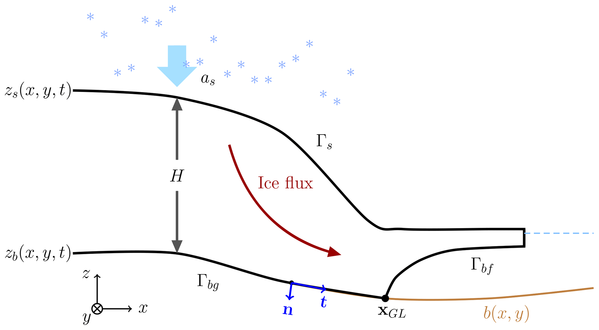
At the boundary Γ of the ice domain Ω we define the normal outgoing vector n and tangential vector t (see Fig. 1). In the 2D vertical case considered here, the ice sheet geometry is constant in y. The ice surface is denoted by Γs and the ice base is . At Γs, and Γbf, the floating part of Γb, we have
respectively. The ice is stress free at Γs, fs=0, and at the ice–ocean interface Γbf, where pw is the water pressure. Let
where σnn and σnt are the normal and tangential components of the stress and ut is the tangential component of the ice velocity at the ice base. Then for the slip boundary Γbg, the grounded part of Γb where the ice rests on the bedrock, we have a friction law for the sliding ice
where un is the normal component of the ice velocity. The type of friction law is determined by the friction coefficient β (≥0). At Γbf, there is a balance between σnn and pw, and the contact is friction free, β=0. Then
At the GL, the boundary condition switches from β>0 and un=0 on Γbg to β=0 and a free un on Γbf. In a 2D vertical cross section of ice, the GL is the point (xGL,zGL) shared between Γbg and Γbf.
The ocean surface is at z=0, and . The density of sea water is denoted by ρw, zb is the z coordinate of Γb, and g is the vertical component of the gravitational force.
2.3 The free-surface equations
The boundaries Γs and Γb are time dependent and move according to two free-surface equations. The boundary Γbg follows the fixed bedrock with coordinates (x,b(x)).
The z coordinate of the ice surface position zs(x,t) at Γs (see Fig. 1) is the solution of an advection equation
where as denotes the surface mass balance and the velocity at the ice surface in contact with the atmosphere. Similarly, the z coordinate for the ice base zb of the floating ice at Γbf satisfies
where ab is the basal mass balance and the velocity of the ice at Γbf. On Γbg, zb=b(x); on Γbf, zb>b(x).
The thickness of the ice is denoted by and depends on x and t.
2.4 A first-order solution close to the grounding line
The 2D vertical solution of the FS equations in Eq. (1) with a constant viscosity, n=1 in Eq. (3), is expanded in small parameters in Schoof (2011). The solutions in different regions around the GL are connected by matched asymptotics. Upstream of the GL at the grounded part, x<xGL, the leading terms in the expansion satisfy a simple relation in scaled variables close to the GL. Across the GL, the ice velocity u, the flux of ice uH, and the depth-integrated normal or longitudinal stress τ11 in Eq. (2) are continuous. By including higher-order terms in the expansion in small parameters, it is shown in Schoof (2011, Sect. 4.7) that the ice surface slope is continuous and Archimedes' flotation condition
is not satisfied immediately downstream of the GL. A rapid variation in the vertical velocity w in a short-distance interval at the GL causes oscillations in the ice surface in the analysis as also observed in FS simulations in Durand et al. (2009a). The flotation condition in Eq. (9) determines where the GL is in SSA in Docquier et al. (2011) and Drouet et al. (2013).
In Schoof (2011, Sect. 4.3), the solution to the FS in a 2D vertical cross section of ice is expanded in two parameters, ν and ϵ. The aspect ratio of the ice ν is the quotient between a typical scale of the thickness of the ice ℋ and a horizontal length scale ℒ, , and ϵ is ν times the quotient between the longitudinal and the shear stresses τ11 and τ12 in Eq. (2). If , then in a boundary layer close to the GL and x<xGL it follows from the equations that the leading terms in the solution in scaled variables satisfy
On floating ice and the hydrostatic flotation criterion Eq. (9) is fulfilled. This is a first-order approximation of the second relation in Eq. (6). On the grounded ice domain, we have .
Introducing the notation
and letting be the thickness of the ice below the sea level yields
If x<xGL, then χa<0 in the neighborhood of xGL on Γbg; if x>xGL then χa=0 and Eq. (9) holds true on Γbf. Suppose that zs and zb are linear in x. Then χa is also linear in x. In numerical experiments with the linear FS (n=1) in Nowicki and Wingham (2008), χa(x,zb) varies linearly in x for x<xGL.
In Sect. 4, we take this same approach but use an indicator χ(x) or derived from the solutions of the nonlinear FS equations to estimate the GL position. These indicators are approximated by χa(x,zb).
In this section we state the weak form of Eq. (1), introduce the spatial FEM discretization used for Eq. (1), and give the time discretization of Eqs. (7) and (8).
3.1 The weak form of the FS equations
We start by defining the mixed weak form of the FS equations. Introduce , with n from Glen's flow law and the spaces
see, for example, Jouvet and Rappaz (2011, Eq. 3.7), Chen et al. (2013, Sect. 3.1), and Martin and Monnier (2014, Eq. 21). The weak solution (u,p) of Eq. (1) is obtained as follows. Find such that for all the equation
is satisfied, where
The last term in B𝒩 is added in the weak form in Nitsche's method (Nitsche, 1971) to impose the Dirichlet condition un=0 weakly on Γbg. It can be considered as a penalty term. Since , the contribution of the tangential force can also be written βu⋅v when un=0. The value of the positive parameter γ0 depends on the physical problem, and h is a measure of the mesh size on Γb. The sensitivity of the GL positions for different values of γ0 is shown in Sect. 5. The first term in B𝒩 symmetrizes the boundary term BΓ+B𝒩 on Γbg and vanishes when un=0. The boundary term FΓ(v) is from the buoyancy force at the ice–ocean interface in EQ. (6) where pw depends on zb on Γbf.
3.2 The discretized FS equations
We employ linear Lagrange elements with Galerkin least-square (GLS) stabilization (Franca and Frey, 1992; Helanow and Ahlkrona, 2018) to avoid spurious oscillations in the pressure using the standard MISMIP setting in Elmer/ICE (Durand et al., 2009a; Gagliardini et al., 2013) approximating solutions in the spaces Vk and in Eq. (13).
The mesh is constructed from a footprint mesh on the ice base and then extruded with the same number of layers equidistantly in the vertical direction according to the thickness of the ice sheet. To simplify the implementation in 2D, the footprint mesh on the ice base consists of N+1 nodes at with x coordinates xi and a constant mesh size .
In general, the GL is somewhere in the interior of an interval , and it crosses the interval boundaries as it moves forward in the advance phase and backward in the retreat phase of the ice. The advantage with Nitsche's method of formulating the boundary conditions is that if then the boundary integral over the interval can be split into two parts in Eq. (14) such that when , and if then . In the GL element, we have
with the integration element ds following Γb. There is a change of the boundary condition in the middle of the FEM element where the GL is located. With a strong formulation of the boundary condition un=0, the basis functions in Vk share this property, and the condition changes from the grounded node xi−1 where the basis function satisfies un=0 to the floating node at xi with a free un without taking the position of the GL inside into account. With the weak formulation in Nitsche's method, the standard basis functions we use do not satisfy un=0 strictly. The boundary condition is imposed on the solution by the additional penalty term multiplied by γ0 in B𝒩 in Eq. (14). A large γ0 will force un to be small. The penalty term may change inside an element as in Eq. (15), where it is not equal to zero only in the grounded part.
The resulting system of nonlinear equations forms a nonlinear complementarity problem (Christensen et al., 1998). The distance d between the base of the ice and the bedrock at time t and at x is
If d>0 on Γbf, then the ice is not in contact with the bedrock and ; if on Γbg, then the ice and the bedrock are in contact and d=0. Hence, the complementarity relation in the vertical direction is
The contact friction law is such that β>0 when x<xGL and β=0 when x>xGL. The complementarity relation along the ice base at x is then the non-negativity of d and
on Γb. In particular, these relations are valid at the nodes x=xj, .
The complementarity condition also holds for un and σnn such that
without any sign constraint on un except for the retreat phase when the ice leaves the ground and un<0.
Similar implementations for contact problems using Nitsche's method are found in Chouly et al. (2017a, b), where the unknowns in the PDEs are the displacement fields instead of the velocity in Eq. (1). Analysis in Chouly et al. (2017a) suggests that Nitsche's method for the contact problem can provide a stable numerical solution with an optimal convergence rate.
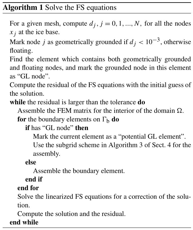
The nonlinear equation Eq. (14), for the nodal values of u and p are solved by Picard iterations. The system of linear equations in every Picard iteration is solved directly by using the MUMPS linear solver in Elmer/ICE. The condition on dj=d(xj) is used to decide if the node xj is geometrically grounded or floating. It is computed at each time step and is not changed during the nonlinear iterations (Picard). The procedure for solution of the nonlinear FS equations is outlined in Algorithm 1. In two dimensions, the GL will be located in one element.
3.3 Discretization of the advection equations
The advection equations for the moving ice boundary in Eqs. (7) and (8) are discretized in time by a finite difference method and in space by FEM with linear Lagrange elements for zs and zb. An artificial diffusion stabilization term is added, making the spatial discretization behave like an upwind scheme in the direction of the velocity as implemented in Elmer/ICE.
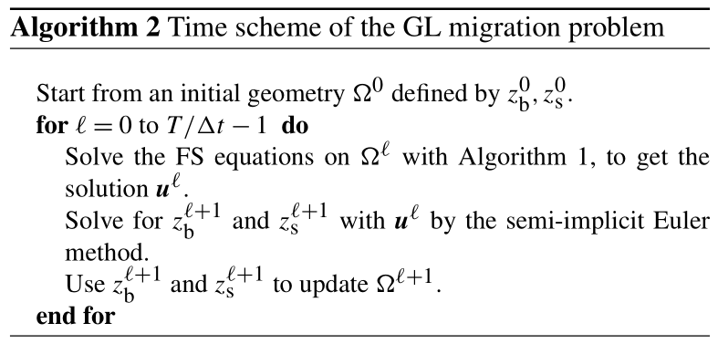
The advection equations Eqs. (7) and (8) are integrated in time by a semi-implicit method of first-order accuracy. Let c=s or b. Then the solution is advanced from time tℓ to with the time step Δt by
The spatial derivative of zc is approximated by FEM as described above. A system of linear equations is solved at tℓ+1 for . This time discretization and its properties are
discussed in Cheng et al. (2017) and summarized in Algorithm 2.
A numerical stability problem in zb is encountered in the boundary condition at Γbf when the FS equations are solved in Durand et al. (2009a). It is resolved by expressing zb in pw at Γbf with a damping term. An alternative interpretation of the idea in Durand et al. (2009a) and an explanation follow below.
The relation between un and ut at Γbf and is
where zbx denotes . Inserting ub and wb from Eq. (21) into Eq. (8) yields
Instead of discretizing Eq. (22) explicitly at tℓ+1 with to determine , the base coordinate is updated implicitly,
in the evaluation of pw in FΓ(v) in Eq. (14).
Assuming that zbx is small, the time step restriction in Eq. (23) is estimated by considering a 2D slab of the floating ice of width Δx and thickness H. Newton's law of motion yields
where is the mass of the slab. Dividing by M, integrating in time for un(tm), letting or ℓ, and approximating the integral by the trapezoidal rule for the quadrature yields
with the parameters
Then insert into Eq. (23). All terms in from time steps i<m are collected in the sum ΔtFm−1. Then Eq. (23) can be written
For small changes in zb in Eq. (24), the explicit method with m=ℓ is stable when Δt is so small that
When H=100 m on the ice shelf, Δt<6.1 s, which is far smaller than the stable steps for Eq. (20). Choosing the implicit scheme with , the bound on Δt is
i.e. there is no bound on positive Δt for stability, but accuracy will restrict Δt.
Much longer stable time steps are possible at the surface and the base of the ice with a semi-implicit method (Eq. 20) and a fully implicit method (Eq. 23) compared to an explicit method. For example, the time step for the problem in Eq. (20) with 1 km mesh size can be up to a couple of months. Therefore, we use the scheme in Eq. (20) for Eqs. (7) and (8) and the scheme in Eq. (23) for Eq. (22) and pw as in Durand et al. (2009a). The difference between the approximations of zb in Eqs. (20) and (23) is 𝒪(Δt2).
The basic idea of the subgrid scheme for the FS equations in this paper follows the GL parameterization (SEP3) for SSA in Seroussi et al. (2014) and the analysis of FS in Schoof (2011). The GL is located at the position where the ice is on the ground and the flotation criterion is perfectly satisfied such that . In the FS equations, the hydrostatic assumption Eq. (9) may not be valid close to the GL. Therefore, the GL position can not be determined by simply checking the total thickness of the ice H against the depth below sea level Hbw. Instead, the flotation criterion is computed by comparing the water pressure with the numerical normal stress component orthogonal to the boundary inspired by the first-order analysis in Sect. 2.4.
The numerical solutions (e.g., Gagliardini et al., 2016; Gladstone et al., 2017) converge to the analytical solution of the FS PDE as the mesh size decreases. The analytical solution satisfies with the boundary conditions in Eq. (6) at the base of the floating ice; where the ice is in contact with the bedrock , the boundary conditions are given by Eq. (5). Examples of the analytical solution are demonstrated by the thin light blue lines in Figs. 2 and 3 with a black “*” at the analytical GL position xGL. The two figures share the same analytical solution. However, as illustrated in Figs. 2 and 3, the basal boundary of the ice zb(x,t) does not conform with the mesh from the spatial discretization. In particular, the GL position xGL of the analytical solution does not coincide with any of the nodes, but it usually stays on the bedrock b(x) between the last grounded (xi−1) and the first floating (xi) nodes; see Figs. 2 and 3. The linear element boundary between any xj−1 and xj is denoted by ℰj. The sequence of , approximates Γb. The grounding line element containing the GL is ℰi.
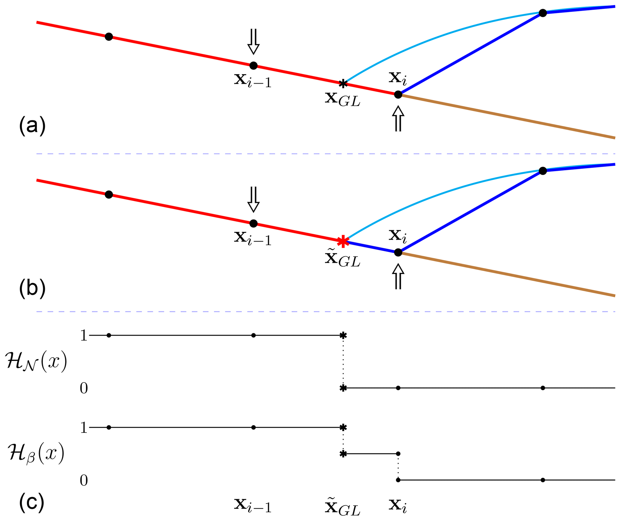
Figure 2Schematic figure of the GL in case i, with the arrows indicating the direction of the net forces in the vertical direction. The light blue line is the analytical solution of the ice sheet with the analytical GL position xGL. The red line is the grounded boundary Γbg, the dark blue line is the floating boundary Γbf, and the brown line is the bedrock topography b(x). (a) The last grounded and first floating nodes as defined in Elmer/ICE. (b) Linear interpolation to approximate the numerical GL position . (c) The step functions ℋ𝒩(x) and ℋβ(x) indicate the area for Nitsche's penalty and slip boundary conditions.
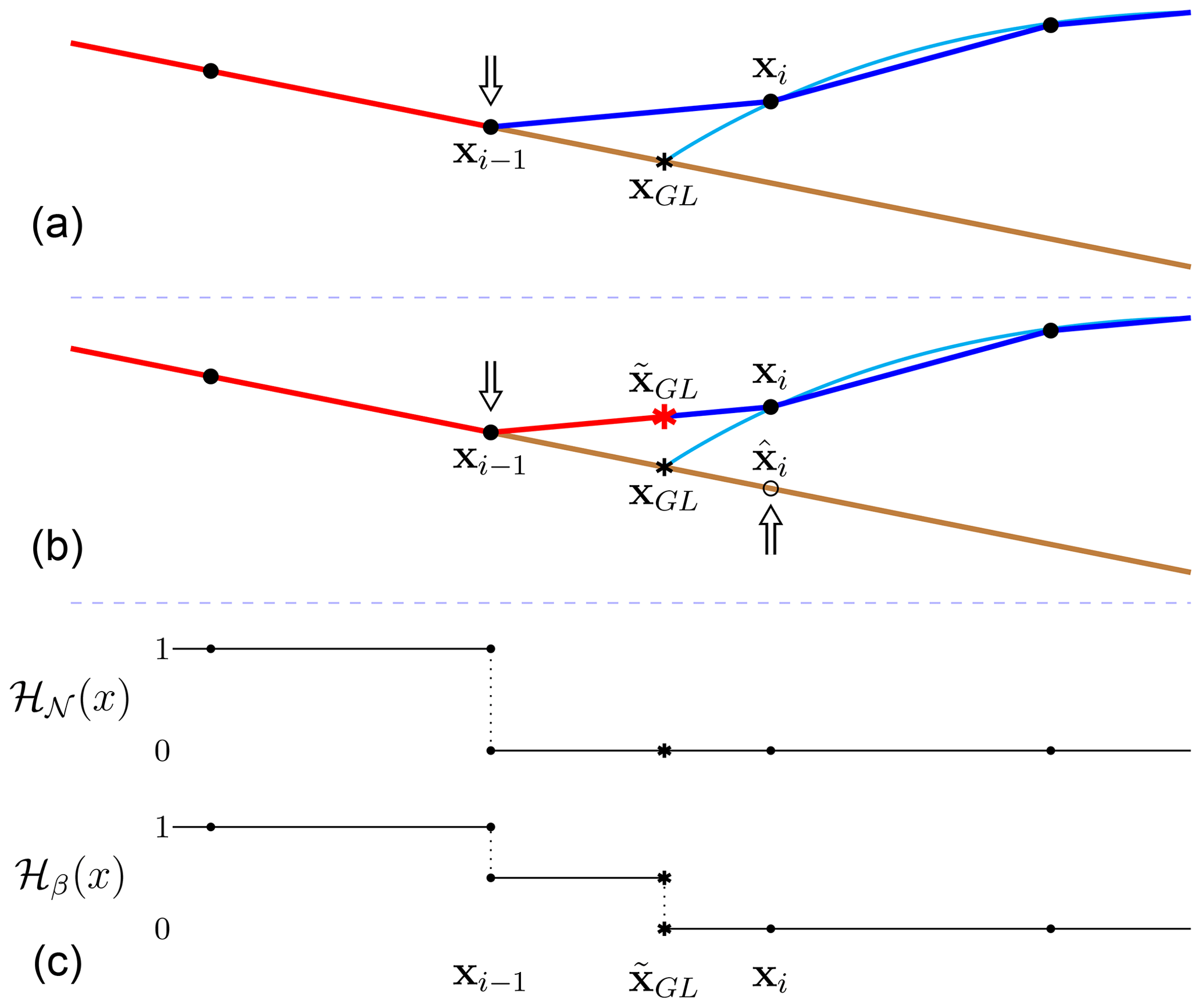
Figure 3Schematic figure of the GL in case ii, with the arrows indicating the direction of the net forces in the vertical direction. The colors of the lines follow those in Fig. 2. (a) The last grounded and first floating nodes as defined in Elmer/ICE. The node xi is fully geometrically floating, and the net force is 0. (b) Linear interpolation to approximate the numerical GL position . The point on the bedrock has the same x coordinate as xi. (c) The step functions ℋ𝒩(x) and ℋβ(x) indicate the area for Nitsche's penalty and slip boundary conditions.
Depending on how the mesh is created from the initial geometry and updated during the simulation, the first floating node at xi, as well as the GL element, can be either on the bedrock (as in Fig. 2) or at the ice base above the bedrock (as in Fig. 3), even though the corresponding analytical solutions are identical. Denote the situation in Fig. 2 as case i and the one in Fig. 3 as case ii. The physical boundary conditions of the two cases are different only at the GL element. More precisely, in case i the net force in the vertical direction on the node xi is pointing inward, namely , whereas in case ii the floating condition is satisfied in the node xi. The directions of the vertical net force at the nodes xi−1 and xi are shown by the arrows in Figs. 2a and 3a. Consequently, the external forces and boundary conditions imposed on the GL element are different in the two cases. For instance, in case i the GL element is considered as geometrically grounded (defined as in Algorithm 1), shown with in red in Fig. 2a. In case ii, the GL element is treated as geometrically floating and colored in blue in Fig. 3a.
These two cases are similar to the LG and FF cases in Gagliardini et al. (2016), implying that the numerical solutions in the two cases are different, especially on a coarse mesh (mesh size of about 100 m or larger). Thus, we propose a subgrid scheme to reduce these differences in the spatial discretization and to capture the GL migration without using a fine mesh resolution (<100 m). The schematic drawing of the subgrid scheme for the two cases is shown in the panels b of Figs. 2 and 3. The GL element is divided into the grounded (red) and floating (blue) parts by the estimated GL position on ℰi, which is the numerical approximation of the analytical GL position xGL.
The GL moves toward the ocean in the advance phase and away from the ocean in the retreat phase. First, we consider case i in the advance phase and define the indicator as
which vanishes on the floating ice and is negative and approximately equal to in Eq. (11) on the ground since the slope of the bedrock is small and . Because of the poor spatial resolution of the coarse mesh, χ(xi) is positive.
To determine the position , we solve by linear interpolation between χ(xi−1) and χ(xi) such that
The water pressure pw(x) is a linear function of x on the GL element, and the numerical solution of σnn(x) is also piecewise linear on every element with the standard Lagrange elements in Elmer/ICE (Gagliardini et al., 2013). Hence, it makes sense to approximate the analytical GL position xGL by by linear interpolation in the current framework. This approach fits well with case i since the indicator χ(x) has opposite signs at xi−1 and xi; see Fig. 2b, where is marked with a red “*”. It guarantees the existence and uniqueness of on the GL element.
Another situation in the advance phase is case ii, shown in Fig. 3. As the elements on both sides of the node xi are geometrically floating, the boundary condition imposed on xi becomes . However, the implicit treatment of the ice base moves the z coordinate of the node xi towards the bedrock with un>0 in Eq. (23) as discussed in Sect. 3.3. The result is that pw defined by the implicit zb in Eq. (23) satisfies in Eq. (27) and χ(xi)>0.
The implicit treatment of the ice base has the consequence that only case ii occurs in the retreat phase. When the FS equations are solved, the implicit update of the ice base with un<0 in Eq. (23) implies that the last grounded node in the previous time step is leaving the bedrock when the ice is retreating and the GL moves back to the adjacent element. Case i will not appear in that situation since zb(xi)>b(xi). In this circumstance, χ(xi)=0 in the floating node and a correction of χ(x) is introduced into case ii by in
Here is the water pressure on the bedrock corresponding to linear extrapolation of the pressure for x>xGL along the element on the bedrock. Furthermore, . Notice that , where is a point on the bedrock with the same x coordinate of xi, as illustrated in Fig. 3b. Both χ(x) in Eq. (27) and in Eq. (29) are nonlinear in x, but the numerical approximation of them will vary linearly in x. A solution is found by linear interpolation of between the nodes xi−1 and xi as in Eq. (28). It follows from Eq. (28) that is located on the element boundary; see Figs. 2 and 3. If we compare with case i, this correction can be considered as using to approximate σnn(xGL) on a virtual element between xi−1 and ; see Fig. 3. The position is a numerical approximation of the analytical GL position, although it is not geometrically in contact with the bedrock.
Since we have pb(x)=pw(x) and at the GL element in case i, we can simply use to find for the two cases by replacing χ in Eq. (28) by .
The domains Γbg and Γbf are separated at as in Eq. (15), and the integrals on the GL element are calculated with a high-order integration scheme as in Seroussi et al. (2014). We introduce two step functions, ℋ𝒩(x) and ℋβ(x), to include and exclude quadrature points in the integration of Nitsche's term and the slip boundary condition, respectively. They are defined for case i in Fig. 2 and for case ii in Fig. 3. To achieve a reasonable numerical accuracy within the GL element, as suggested in Seroussi et al. (2014), at least 10th-order Gaussian quadrature is used.
The penalty term in Nitsche's method restricts the motion of the element in the normal direction. It is only imposed on an element which is fully geometrically on the ground in case i. In contrast, in case ii the GL element ℰi is not in contact with the bedrock; see Fig. 3. The normal velocity on the element should not be forced to zero, and only the floating boundary condition is then used on the GL element. Nitsche's penalty term should be imposed on all the fully geometrically grounded elements and partially on the GL element in the advance phase as in case i. The step function ℋ𝒩(x) indicates how Nitsche's method is implemented on the basal elements; see Figs. 2c and 3c for the two cases. The penalty term contributes to the integration only when ℋ𝒩(x)=1.
The slip coefficient β is treated similarly with the step function ℋβ(x), where ℋβ(x)=1 is on the fully geometrically grounded elements and ℋβ(x)=0 on the floating elements. To further smooth the transition of β at the GL, the step function is set to be 1∕2 in parts of the GL element before integrating using the high-order scheme. The convergence of the nonlinear iterations is improved in this way. In case i, full friction is applied at the grounded part between xi−1 and of the GL element since this part is also geometrically grounded in the analytical solution of the FS as in Fig. 2. Then, the friction is lower in the remaining part of ℰi. For the floating part between and xi in case ii, there is no friction, ℋβ(x)=0, we have reduced friction between xi−1 and ; see Fig. 3c. The boundary integral Eq. (15) on ℰi is now rewritten with the two step functions as
A summary of the numerical treatment of the GL is as follows:
-
advance phase ⇒ indicator χ in Eq. (27), case i or case ii;
-
retreat phase ⇒ indicator in Eq. (29), case ii.
The case is determined by the geometry of the GL element and the sign of the indicator χ.
The algorithm for the GL element is as follows:
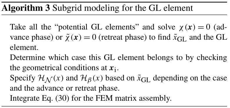
Equations (1), (7), and (8) form a system of coupled nonlinear equations. They are solved by Elmer/ICE v.8.3 in the same manner as Durand et al. (2009b) and Gagliardini et al. (2013, 2016). The detailed procedure is explained in Algorithms 1, 2, and 3. The solution to the nonlinear FS system is computed with Picard iterations to a 10−5 relative error with a limit of maximal 25 nonlinear iterations. The position is determined dynamically during each fixed-point iteration by solving Eq. (28) with χ or and the solution σnn(x) from the previous nonlinear iteration, and the step functions ℋ𝒩 and ℋβ are adjusted accordingly. The water pressure pb is fixed since the ice geometry is not changed during the nonlinear iterations.
The numerical experiments follow the MISMIP benchmark (Pattyn et al., 2012), and a comparison is made with the results in Gagliardini et al. (2016). Using the experiment MISMIP 3a, the setups are exactly the same as in the advancing and retreating simulations in Gagliardini et al. (2016). The experiments are run with spatial resolutions of Δx=4, 2, 1, and 0.5 km. The mesh at the base is extruded vertically in 20 layers with equidistantly placed nodes in each vertical column. The time step is Δt=0.125 year for all four resolutions to eliminate time discretization errors when comparing different spatial resolutions.
The dependence on γ0 in Eq. (30) for the retreating ice is shown in Fig. 4 with γ0 between 104 and 109. The estimated GL positions do not vary with different choices of γ0 from 105 to 108, which suggests a suitable range of γ0. If γ0 is too small (γ0≪104), oscillations appear in the estimated GL positions. If γ0 is too large (γ0≫108), then more nonlinear iterations in Algorithm 1 are needed in each time step. The same dependency of γ0 is observed for the advancing experiments and for different mesh resolutions as well. The results are not very sensitive to γ0 and for the remaining experiments we choose γ0=106.
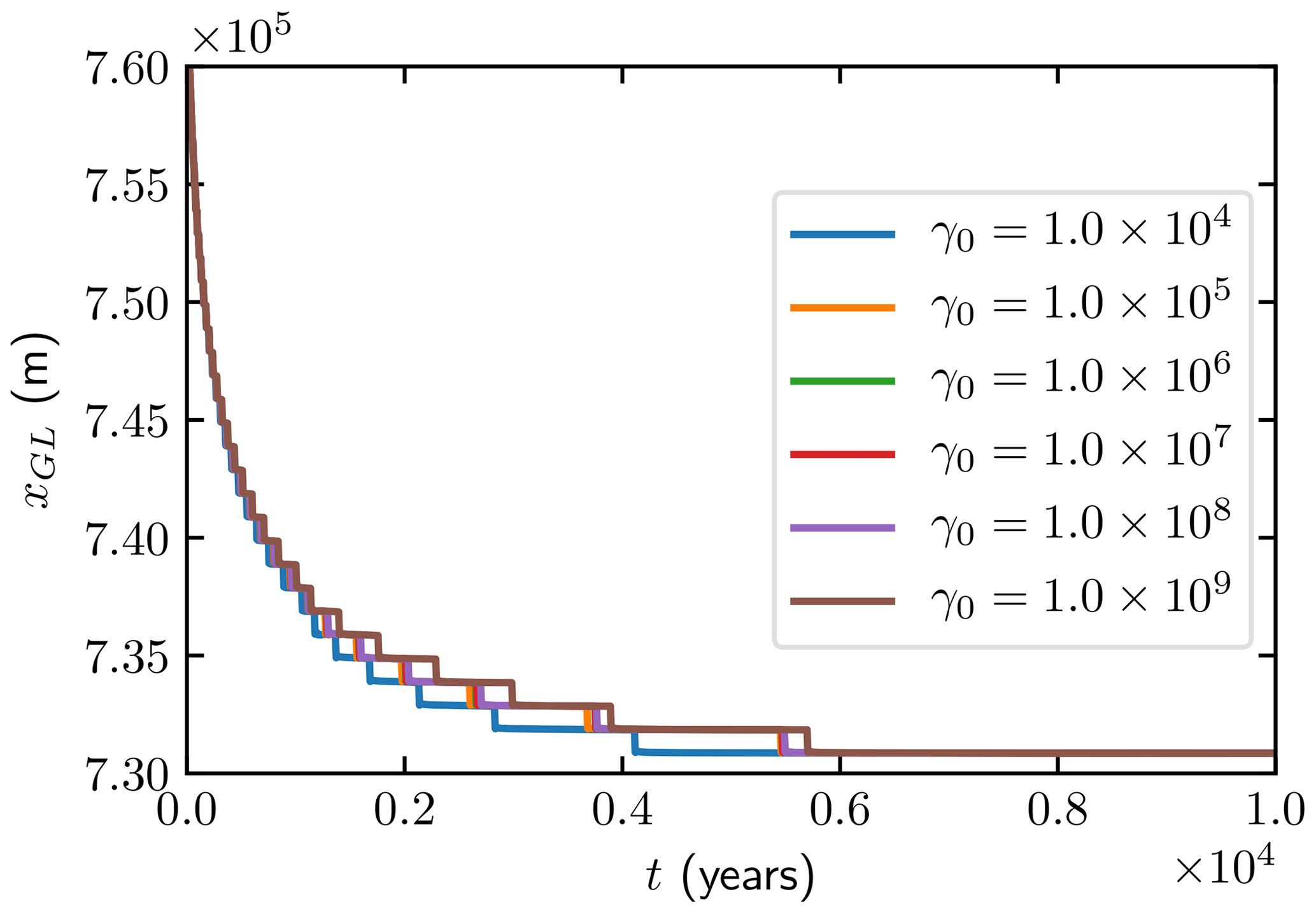
Figure 4The MISMIP 3a retreat experiment with Δx=1 km for different choices of γ0 in the time interval [0,10 000] years.
The GL position during the transient simulations in the advance and retreat phases is displayed in Fig. 5, and the steady-state results (at t=10 000) are shown in Fig. 6 for different mesh resolutions. The range of the steady-state solutions from Gagliardini et al. (2016) with mesh resolution from 25 to 200 m are shown as background shaded regions in red. We achieve similar GL migration results for both the advance and retreat experiments with at least 20-times-larger mesh resolutions. The GL position is insensitive to the variation in mesh size between 0.5 and 4 km.
The distance between the steady-state GL positions of the retreat and the advance phases is shown in Fig. 6b. The maximal distance is about 6 km at Δx=1 km with the subgrid model, whereas in Gagliardini et al. (2016) the resolution has to be below 50 m to achieve a similar result.

Figure 5The MISMIP 3a experiments for the GL position when with Δx=4, 2, 1, and 0.5 km for the advance (solid) and retreat (dashed) phases.
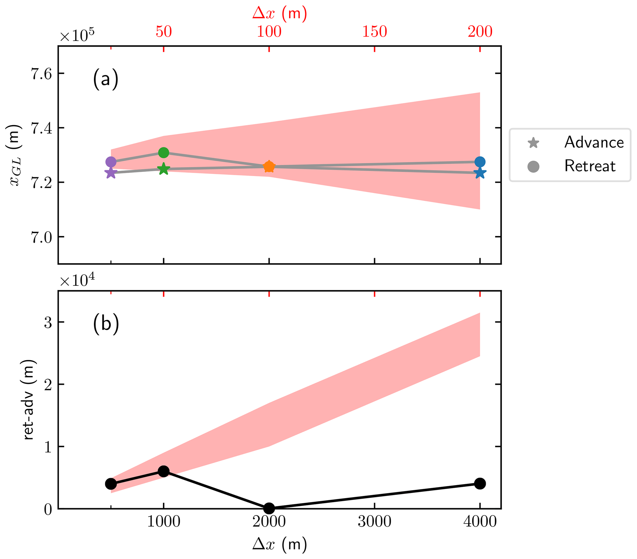
Figure 6The MISMIP 3a experiments at the final time t=10 000 with the resolutions at Δx=4, 2, 1, and 0.5 km. (a) The GL positions in the advance (★) and retreat (•) phases. (b) The distance between the retreat and the advance xGL at the steady states. The shaded regions indicate the range of the results in Gagliardini et al. (2016) with 20-times-smaller mesh resolutions from 25 to 200 m, with the axis scale shown in red at the top of the plot.
We observe oscillations at the ice surface near the GL in all the experiments as expected from Durand et al. (2009a) and Schoof (2011). A zoomed-in plot of the surface elevation computed with four different mesh sizes (Δx=0.5, 1, 2, and 4 km) after an advance simulation to t=10 000 years is found in Fig. 7a. The abscissa is the distance from the steady-state GL position for each mesh size. In general, the estimated GL position does not coincide with any nodes even at the steady state, but it may be close to a node.

Figure 7Details of the solutions for the advance experiment with km after 10 000 years. The solid dots represent the nodes of the elements, and the vertical, dashed red lines indicate the GL position. (a) The oscillations in zs at the ice surface near GL. (b) The flotation criterion is evaluated by Hbw∕H. The ratio ρ∕ρw is drawn in a horizontal, dash-dotted purple line.
The ratio between the thickness below sea level Hbw and the ice thickness H is shown in Fig. 7b. As in Fig. 7a, the ratio is plotted versus the distance from the GL achieved with the particular mesh size. The horizontal, dash-dotted purple line represents the ratio of ρ∕ρw. The solutions vary smoothly over the mesh with Δx=0.5 km, which appears to be a sufficient resolution in both panels of Fig. 7. Moreover, the solutions converge regularly toward the solution with Δx=0.5 km when the mesh size decreases.
The result for Δx=0.5 km in panel b confirms that the hydrostatic assumption Hρ=Hbwρw in Eq. (9) is not valid in the FS equations for x>xGL close to the GL and at the GL position (cf. Durand et al., 2009a; Schoof, 2011). For x<xGL we have since Hbw decreases and H increases. The conclusion from numerical experiments in van Dongen et al. (2018) is that the hydrostatic assumption and the SSA equations approximate the FS equations well for the floating ice beginning at a short distance away from the GL.
The surface and the base velocity solutions from the advance experiment are displayed in Fig. 8 with Δx=0.5, 1, 2, and 4 km after 10 000 years. The horizontal velocities on the two surfaces are on top of each other for all Δx with negligibly small differences on the floating ice as expected. The vertical velocities w on the surface (dotted curves) and the base (solid curves) at the GL are almost discontinuous as analyzed in Schoof (2011). With the subgrid model, the rapid variation is captured with Δx=0.5 km. The convergence for decreasing mesh size behaves smoothly.
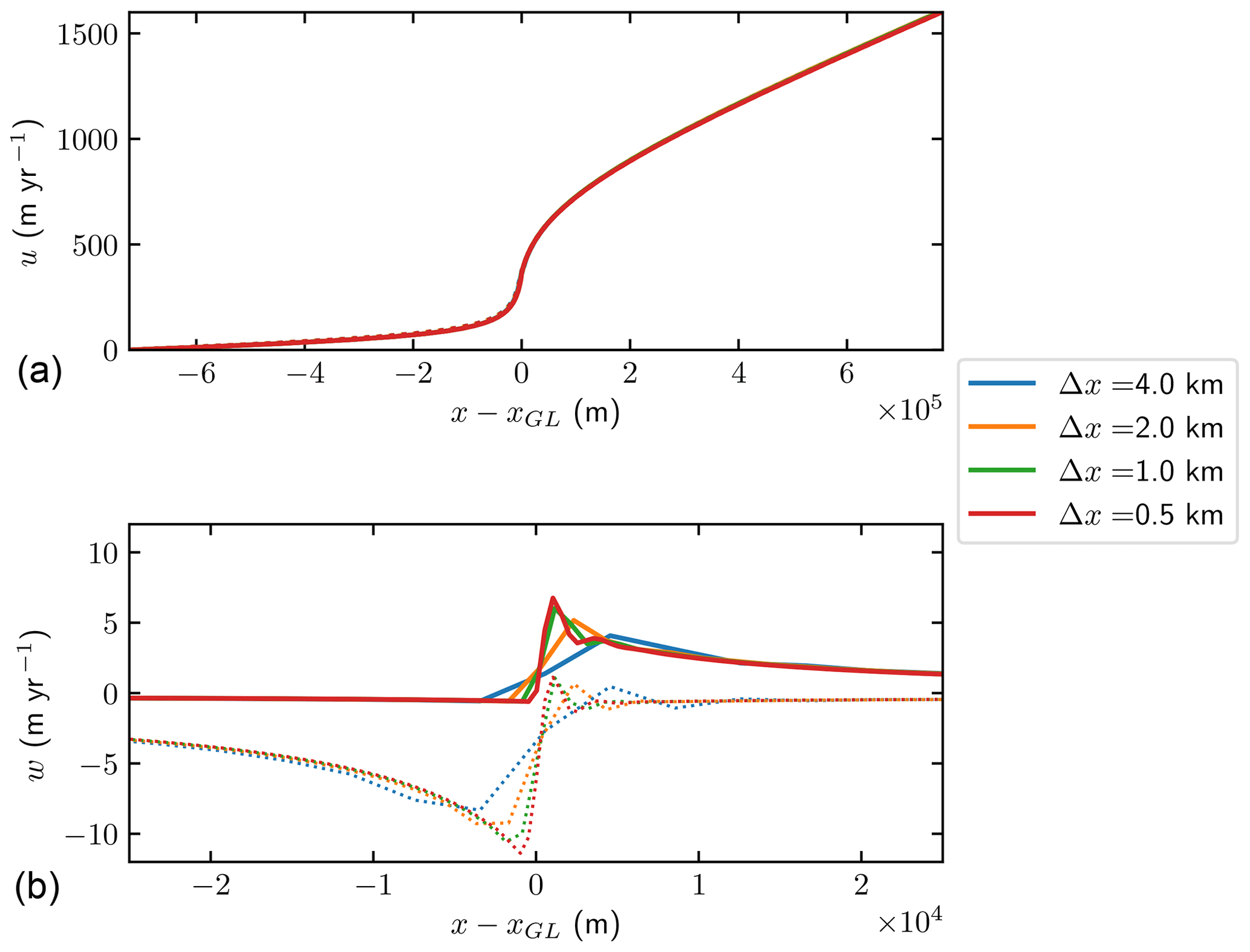
Figure 8The velocities u (a) and w (b) of the ice in the advance experiment with Δx=0.5, 1, 2, and 4 km after 10 000 years. The solutions at the upper surface are the solid curves, and the solutions at the lower surface are the dotted curves. The vertical velocity w is zoomed in close to the GL, with the distance to the mesh-dependent GL on the x axis.
Seroussi et al. (2014) describe four different subgrid models (NSEP, SEP1, SEP2, and SEP3) for the friction in SSA and evaluate them in a FEM discretization on a triangulated, planar domain. The flotation criterion is applied at the nodes of the triangles. In the NSEP, an element is floating or not depending on how many of the nodes of that element are floating. In the other three methods, an inner structure in the triangular element is introduced. One part of a triangle is floating and one part is grounded. The amount of friction in a triangle with the GL is determined by the flotation criterion. The friction coefficient is reduced, the integration in the element only includes the grounded part, or a higher-order polynomial integration (SEP3) is applied. Faster convergence as the mesh is refined is observed for the latter methods compared to the first method. The discretization of the friction in Sect. 4 is similar to the SEP3 method, but the FS equations also require a subgrid treatment of the normal velocity condition. In the method for the FS equations in Gagliardini et al. (2016), the GL position is in a node, and the friction coefficient is approximated in three different ways. The coefficient is discontinuous at the node in one case (DI in Gagliardini et al., 2016). Our coefficient is also discontinuous but at the estimated location of the GL between the nodes.
The convergence of the steady-state GL position toward the reference solutions in Gagliardini et al. (2016) is observed in the simulations in Figs. 5 and 6. However, as the meshes we used are at least 20 times larger than the 25 m finest resolution in Gagliardini et al. (2016), it has probably not reached the convergence asymptote. At the current resolutions, the discretization introduces a strong mesh effect such as the two different geometrical interpretations in the two cases mentioned in Sect. 4. The subgrid scheme is able to provide a more accurate representation of the GL position and the boundary conditions, but the numerical solution of the velocity field, pressure, and two free surfaces are still computed on the coarse mesh, which are the main sources of the numerical errors. Additional uncertainty at the GL is introduced by the approximation of the bedrock geometry, the friction at the GL, and the modeling of the ice–ocean interaction. It is shown in Cheng and Lötstedt (2020) that the solution at the GL is particularly sensitive to variation in the geometry and friction at the ice base.
Our method can be extended to a triangular mesh covering Γb in the following way (considering linear Lagrange functions). The condition on χ in Eq. (27) or in Eq. (29) is applied on the edges of each triangle 𝒯 in the mesh. If χ<0 in all three nodes, then 𝒯 is grounded. If χ≥0 in all nodes, then 𝒯 is floating. The GL passes inside 𝒯 if χ has a different sign in one of the nodes. Then the GL crosses the two edges where χ<0 in one node and χ≥0 in the other node. In this way, a continuous reconstruction of a piecewise linear GL is possible on Γb. The same tests are applied to . The FEM approximation is modified in the same manner as in Sect. 4 using step functions in Nitsche's method.
An alternative to a subgrid scheme is to introduce static or dynamic adaptation of the mesh on Γb with a refinement at the GL as in, for example, Gladstone et al. (2010a), Cornford et al. (2013), and Drouet et al. (2013). In general, a fine mesh is needed at the GL and in an area surrounding it. Since the GL moves long distances in simulations of paleo-ice sheets, the adaptation should be dynamic, permit refinement and coarsening of the mesh varying in time, and be based on some estimate of the numerical error of the method. In shorter time intervals, a static adaptation may be sufficient since the GL will move a shorter distance. Furthermore, shorter time steps are necessary for numerical stability in static and dynamic mesh adaptation schemes. A static adaptation is determined once before the simulation starts. Introducing a time-dependent, dynamic mesh with adaptivity into an existing code requires a substantial coding effort and will increase the computational work considerably compared to a static mesh. Subgrid modeling is easier to implement, and the increase in computing time is small. A combination of dynamic mesh adaptation and subgrid discretization may be the ultimate solution. Then the mesh at the GL would be adapted to resolve the variation in the interior of the ice at the GL, while the subgrid modeling would handle the discontinuity at the basal boundary.
A subgrid scheme at the GL was developed and tested in the SSA model for 2D vertical ice flow in Gladstone et al. (2010b) and in Seroussi et al. (2014), for the friction in the vertically integrated model BISICLES (Cornford et al., 2013) for 2D flow in Cornford et al. (2016), and for the PISM model mixing SIA with SSA in 3D in Feldmann et al. (2014). Here we propose a subgrid scheme for the FS equations for a 2D vertical cross section of ice, implemented in Elmer/ICE, that can be extended to 3D. The mesh is static, and the moving GL position within one element is determined by linear interpolation with an auxiliary function χ(x) or . Only in that element is the FEM discretization modified to accommodate the discontinuities in the boundary conditions. The numerical scheme is applied to the simulation of a 2D vertical ice sheet with an advancing GL and one with a retreating GL. The model setups for the tests are the same as in one of the MISMIP examples (Pattyn et al., 2012) and in Gagliardini et al. (2016). The solution converges smoothly in the neighborhood of the GL when the mesh size is reduced. Comparable results to Gagliardini et al. (2016) are obtained using the subgrid scheme with more than 20-times-larger mesh sizes. A larger mesh size also allows a longer time step for the time integration.
The FS subgrid model is implemented based on Elmer/ICE (Gagliardini et al., 2013) Version 8.3 (SHA-1: f6bfdc9) which is available for download under GitHub (https://github.com/ElmerCSC/elmerfem, last access: 11 May 2020).The revision used in this work can be downloaded from https://github.com/enigne/elmerfem/archive/v1.0.0.zip (last access: 6 September 2019) and https://github.com/enigne/elmerfem/archive/v1.0.1.zip (last access: 6 September 2019).
GC developed the model code and performed the simulations. GC and PL contributed to the theory of the paper. GC, PL, and LvS contributed to the development of the method and the writing of the paper.
The authors declare that they have no conflict of interest.
We are grateful to Thomas Zwinger for advice and help in the implementation of the subgrid scheme in Elmer/ICE. The computations were performed on resources provided by the Swedish National Infrastructure for Computing (SNIC) at the PDC Center for High Performance Computing, KTH Royal Institute of Technology. We also thank the anonymous referees for their helpful comments.
This research has been supported by the Svenska Forskningsråadet Formas (grant no. 2017-00665) to Nina Kirchner and the Swedish strategic research program eSSENCE.
This paper was edited by Alexander Robel and reviewed by three anonymous referees.
Brondex, J., Gagliardini, O., Gillet-Chaulet, F., and Durand, G.: Sensitivity of grounding line dynamics to the choice of the friction law, J. Glaciol., 63, 854–866, 2017. a
Chen, Q., Gunzburger, M., and Perego, M.: Well-posedness results for a nonlinear Stokes problem arising in glaciology, SIAM J. Math. Anal., 45, 2710–2733, 2013. a
Cheng, G. and Lötstedt, P.: Parameter sensitivity analysis of dynamic ice sheet models – numerical computations, The Cryosphere, 14, 673–691, https://doi.org/10.5194/tc-14-673-2020, 2020. a
Cheng, G., Lötstedt, P., and von Sydow, L.: Accurate and stable time stepping in ice sheet modeling, J. Comput. Phys., 329, 29–47, 2017. a
Chouly, F., Fabre, M., Hild, P., Mlika, R., Pousin, J., and Renard, Y.: An overview of recent results on Nitsche’s method for contact problems, in: Geometrically unfitted finite element methods and applications, Springer, 93–141, 2017a. a, b, c
Chouly, F., Hild, P., Lleras, V., and Renard, Y.: Nitsche-based finite element method for contact with Coulomb friction, in: European Conference on Numerical Mathematics and Advanced Applications, Springer, 839–847, 2017b. a
Christensen, P. W., Klarbring, A., Pang, J. S., and Strömberg, N.: Formulation and comparison of algorithms for frictional contact problems, Int. J. Num. Meth. Eng., 42, 145–173, 1998. a
Cornford, S., Martin, D., Lee, V., Payne, A., and Ng, E.: Adaptive mesh refinement versus subgrid friction interpolation in simulations of Antarctic ice dynamics, Ann. Glaciol., 57, 1–9, 2016. a, b
Cornford, S. L., Martin, D. F., Graves, D. T., Ranken, D. F., Brocq, A. M. L., Gladstone, R. M., Payne, A. J., Ng, E. G., and Lipscomb, W. H.: Adaptive mesh, finite volume modeling of marine ice sheets, J. Comput. Phys., 232, 529–549, 2013. a, b, c
DeConto, R. M. and Pollard, D.: Contribution of Antarctica to past and future sea-level rise, Nature, 531, 591–597, 2016. a
Docquier, D., Perichon, L., and Pattyn, F.: Representing grounding line dynamics in numerical ice sheet models: Recent advances and outlook, Surv. Geophys., 32, 417–435, 2011. a, b
Drouet, A. S., Docquier, D., Durand, G., Hindmarsh, R., Pattyn, F., Gagliardini, O., and Zwinger, T.: Grounding line transient response in marine ice sheet models, The Cryosphere, 7, 395–406, https://doi.org/10.5194/tc-7-395-2013, 2013. a, b
Durand, G. and Pattyn, F.: Reducing uncertainties in projections of Antarctic ice mass loss, The Cryosphere, 9, 2043–2055, https://doi.org/10.5194/tc-9-2043-2015, 2015. a
Durand, G., Gagliardini, O., de Fleurian, B., Zwinger, T., and Le Meur, E.: Marine ice sheet dynamics: Hysteresis and neutral equilibrium, J. Geophys. Res.-Earth, 114, F03009, https://doi.org/10.1029/2008JF001170, 2009a. a, b, c, d, e, f, g, h
Durand, G., Gagliardini, O., Zwinger, T., Le Meur, E., and Hindmarsh, R. C. A.: Full Stokes modeling of marine ice sheets: influence of the grid size, Ann. Glaciol., 50, 109–114, 2009b. a, b, c
Feldmann, J., Albrecht, T., Khroulev, C., Pattyn, F., and Levermann, A.: Resolution-dependent performance of grounding line motion in a shallow model compared with a full-Stokes model according to the MISMIP3d intercomparison, J. Glaciol., 60, 353–360, 2014. a, b
Franca, L. P. and Frey, S. L.: Stabilized finite element methods: II. The incompressible Navier-Stokes equations, Comput. Meth. Appl. Mech. Eng., 99, 209–233, 1992. a
Gagliardini, O., Zwinger, T., Gillet-Chaulet, F., Durand, G., Favier, L., de Fleurian, B., Greve, R., Malinen, M., Martín, C., Råback, P., Ruokolainen, J., Sacchettini, M., Schäfer, M., Seddik, H., and Thies, J.: Capabilities and performance of Elmer/Ice, a new-generation ice sheet model, Geosci. Model Dev., 6, 1299–1318, https://doi.org/10.5194/gmd-6-1299-2013, 2013 (data available at: https://github.com/ElmerCSC/elmerfem, last access: 11 May 2020). a, b, c, d, e, f
Gagliardini, O., Brondex, J., Gillet-Chaulet, F., Tavard, L., Peyaud, V., and Durand, G.: On the substantial influence of thetreatment of friction at the grounding line, The Cryosphere Discuss., 9, 3475–3501, 2015. a
Gagliardini, O., Brondex, J., Gillet-Chaulet, F., Tavard, L., Peyaud, V., and Durand, G.: Brief communication: Impact of mesh resolution for MISMIP and MISMIP3d experiments using Elmer/Ice, The Cryosphere, 10, 307–312, https://doi.org/10.5194/tc-10-307-2016, 2016. a, b, c, d, e, f, g, h, i, j, k, l, m, n
Gladstone, R. M., Lee, V., Vieli, A., and Payne, A. J.: Grounding line migration in an adaptive mesh ice sheet model, J. Geophys. Res., 115, F04014, https://doi.org/10.1029/2009JF001615, 2010a. a
Gladstone, R. M., Payne, A. J., and Cornford, S. L.: Parameterising the grounding line in flow-line ice sheet models, The Cryosphere, 4, 605–619, https://doi.org/10.5194/tc-4-605-2010, 2010b. a, b
Gladstone, R. M., Warner, R. C., Galton-Fenzi, B. K., Gagliardini, O., Zwinger, T., and Greve, R.: Marine ice sheet model performance depends on basal sliding physics and sub-shelf melting, The Cryosphere, 11, 319–329, https://doi.org/10.5194/tc-11-319-2017, 2017. a, b
Gong, Y., Zwinger, T., Cornford, S., Gladstone, R., Schäfer, M., and Moore, J. C.: Importance of basal boundary conditions in transient simulations: case study of a surging marine-terminating glacier on Austfonna, Svalbard, J. Glaciol., 63, 106–117, 2017. a
Hanna, E., Navarro, F. J., Pattyn, F., Domingues, C. M., Fettweis, X., Ivins, E. R., Nicholls, R. J., Ritz, C., Smith, B., Tulaczyk, S., Whitehouse, P. L., and Zwally, H. J.: Ice-sheet mass balance and climate change, Nature, 498, 51–59, 2013. a
Helanow, C. and Ahlkrona, J.: Stabilized equal low-order finite elements in ice sheet modeling–accuracy and robustness, Comput. Geosci., 22, 951–974, 2018. a
Hutter, K.: Theoretical Glaciology, D. Reidel Publishing Company, Terra Scientific Publishing Company, Dordrecht, 1983. a
Jouvet, G. and Rappaz, J.: Analysis and finite element approximation of a nonlinear stationary Stokes problem arising in glaciology, Adv. Numer. Anal., 2011, 164581, https://doi.org/10.1155/2011/164581, 2011. a
Kingslake, J., Scherer, R. P., Albrecht, T., Coenen, J., Powell, R. D., Reese, R., Stansell, N. D., Tulaczyk, S., Wearing, M. G., and Whitehouse, P. L.: Extensive retreat and re-advance of the West Antarctic ice sheet during the Holocene, Nature, 558, 430–434, 2018. a
Konrad, H., Shepherd, A., Gilbert, L., Hogg, A. E., McMillan, M., Muir, A., and Slater, T.: Net retreat of Antarctic glacier grounding line, Nat. Geosci., 11, 258–262, 2018. a
Larour, E., Seroussi, H., Adhikari, S., Ivins, E., Caron, L., Morlighem, M., and Schlegel, N.: Slowdown in Antarctic mass loss from solid Earth and sea-level feedbacks, Science, 364, eaav7908, https://doi.org/10.1126/science.aav7908, 2019. a
Leguy, G. R., Asay-Davis, X. S., and Lipscomb, W. H.: Parameterization of basal friction near grounding lines in a one-dimensional ice sheet model, The Cryosphere, 8, 1239–1259, https://doi.org/10.5194/tc-8-1239-2014, 2014. a
Leng, W., Ju, L., Gunzburger, M., Price, S., and Ringler, T.: A parallel high-order accurate finite element nonlinear Stokes ice sheet model and benchmark experiments, J. Geophys. Res.-Earth, 117, 2156–2202, 2012. a
MacAyeal, D. R.: Large-scale ice flow over a viscous basal sediment: Theory and application to Ice Stream B, Antarctica., J. Geophys. Res., 94, 4071–4078, 1989. a
Martin, N. and Monnier, J.: Four-field finite element solver and sensitivities for quasi-Newtonian flows, SIAM J. Sci. Compu., 36, S132–S165, 2014. a
Nitsche, J.: Über ein Variationsprinzip zur Lösung von Dirichlet-Problemen bei Verwendung von Teilräumen, die keinen Randbedingungen unterworfen sind, Abh. Math. Semin., University of Hamburg, Germany, 36, 9–15, 1971. a, b
Nowicki, S. M. J. and Wingham, D. J.: Conditions for a steady ice sheet–ice shelf junction, Earth Planet. Sc. Lett., 265, 246–255, 2008. a
Pattyn, F. and Durand, G.: Why marine ice sheet model predictions may diverge in estimating future sea level rise, Geophys. Res. Lett., 40, 4316–4320, 2013. a
Pattyn, F., Schoof, C., Perichon, L., Hindmarsh, R. C. A., Bueler, E., de Fleurian, B., Durand, G., Gagliardini, O., Gladstone, R., Goldberg, D., Gudmundsson, G. H., Huybrechts, P., Lee, V., Nick, F. M., Payne, A. J., Pollard, D., Rybak, O., Saito, F., and Vieli, A.: Results of the Marine Ice Sheet Model Intercomparison Project, MISMIP, The Cryosphere, 6, 573–588, https://doi.org/10.5194/tc-6-573-2012, 2012. a, b, c
Pattyn, F., Perichon, L., Durand, G., Favier, L., Gagliardini, O., Hindmarsh, R. C. A., Zwinger, T., Albrecht, T., Cornford, S., Docquier, D., Fürst, J. J., Goldberg, D., Gudmundsson, G. H., Humbert, A., Hütten, M., Jouvet, G., Kleiner, T., Larour, E., Martin, D., Morlighem, M., Payne, A. J., Pollard, D., Rückamp, M., Rybak, O., Seroussi, H., Thoma, M., and Wilkens, N.: Grounding-line migration in plan-view marine ice-sheet models: results of the ice2sea MISMIP3d intercomparison, J. Glaciol., 59, 410–422, 2013. a, b, c
Reusken, A., Xu, X., and Zhang, L.: Finite element methods for a class of continuum models for immiscible flows with moving contact lines, Int. J. Numer. Meth. Fl., 84, 268–291, 2017. a
Schoof, C.: Marine ice sheet dynamics. Part 2. A Stokes flow contact problem, J. Fluid Mech., 679, 122–155, 2011. a, b, c, d, e, f, g, h, i, j
Schoof, C. and Hindmarsh, R.: Thin-Film Flows with Wall Slip: An Asymptotic Analysis of Higher Order Glacier Flow Models, Q. J. Mech. Appl. Math., 63, 73–114, 2010. a
Seroussi, H., Morlighem, M., Larour, E., Rignot, E., and Khazendar, A.: Hydrostatic grounding line parameterization in ice sheet models, The Cryosphere, 8, 2075–2087, https://doi.org/10.5194/tc-8-2075-2014, 2014. a, b, c, d, e, f
Stokes, C. R., Tarasov, L., Blomdin, R., Cronin, T. M., Fisher, T. G., Gyllencreutz, R., Hättestrand, C., Heyman, J., Hindmarsh, R. C. A., Hughes, A. L. C., Jakobsson, M., Kirchner, N., Livingstone, S. J., Margold, M., Murton, J. B., Noormets, R., Peltier, W. R., Peteet, D. M., Piper, D. J. W., Preusser, F., Renssen, H., Roberts, D. H., Roche, D. M., Saint-Ange, F., and Stroeven, A. P.: On the reconstruction of palaeo-ice sheets: Recent advances and future challenges, Quaternary Sci. Rev., 125, 15–49, 2015. a
Urquiza, J. M., Garon, A., and Farinas, M.-I.: Weak imposition of the slip boundary condition on curved boundaries for Stokes flow, J. Comput. Phys., 256, 748–767, 2014. a
van Dongen, E. C. H., Kirchner, N., van Gijzen, M. B., van de Wal, R. S. W., Zwinger, T., Cheng, G., Lötstedt, P., and von Sydow, L.: Dynamically coupling full Stokes and shallow shelf approximation for marine ice sheet flow using Elmer/Ice (v8.3), Geosci. Model Dev., 11, 4563–4576, https://doi.org/10.5194/gmd-11-4563-2018, 2018. a
Wilchinsky, A. V. and Chugunov, V. A.: Ice-stream–ice-shelf transition: theoretical analysis of two-dimensional flow, Ann. Glaciol., 30, 153–162, 2000. a
Zhang, T., Price, S., Ju, L., Leng, W., Brondex, J., Durand, G., and Gagliardini, O.: A comparison of two Stokes ice sheet models applied to the Marine Ice Sheet Model Intercomparison Project for plan view models (MISMIP3d), The Cryosphere, 11, 179–190, https://doi.org/10.5194/tc-11-179-2017, 2017. a