the Creative Commons Attribution 4.0 License.
the Creative Commons Attribution 4.0 License.
 | 07 May 2020
Evaluating a fire smoke simulation algorithm in the National Air Quality Forecast Capability (NAQFC) by using multiple observation data sets during the Southeast Nexus (SENEX) field campaign
HyunCheol Kim
Pius Lee
Rick Saylor
YouHua Tang
Daniel Tong
Barry Baker
Shobha Kondragunta
Chuanyu Xu
Mark G. Ruminski
Weiwei Chen
Jeff Mcqueen
Ivanka Stajner
Multiple observation data sets – Interagency Monitoring of Protected Visual Environments (IMPROVE) network data, the Automated Smoke Detection and Tracking Algorithm (ASDTA), Hazard Mapping System (HMS) smoke plume shapefiles and aircraft acetonitrile (CH3CN) measurements from the NOAA Southeast Nexus (SENEX) field campaign – are used to evaluate the HMS–BlueSky–SMOKE (Sparse Matrix Operator Kernel Emission)–CMAQ (Community Multi-scale Air Quality Model) fire emissions and smoke plume prediction system. A similar configuration is used in the US National Air Quality Forecasting Capability (NAQFC). The system was found to capture most of the observed fire signals. Usage of HMS-detected fire hotspots and smoke plume information was valuable for deriving both fire emissions and forecast evaluation. This study also identified that the operational NAQFC did not include fire contributions through lateral boundary conditions, resulting in significant simulation uncertainties. In this study we focused both on system evaluation and evaluation methods. We discussed how to use observational data correctly to retrieve fire signals and synergistically use multiple data sets. We also addressed the limitations of each of the observation data sets and evaluation methods.
- Article
(16514 KB) - Full-text XML
- BibTeX
- EndNote


Wildfires and agricultural/prescribed burns are common in North America all year round but predominantly occur during the spring and summer months (Wiedinmyer et al., 2006). These fires pose a significant risk to air quality and human health (Delfino et al., 2009; Rappold et al., 2011; Dreessen et al., 2016; Wotawa and Trainer, 2000; Sapkota et al., 2005; Jaffe et al., 2013; Johnston et al., 2012). Since January 2015, smoke emissions from fires have been included in the National Air Quality Forecasting Capability (NAQFC) daily PM2.5 operational forecast (Lee et al., 2017). The NAQFC fire simulation consists of the NOAA National Environmental and Satellite Data and Information Service (NESDIS) Hazard Mapping System (HMS) fire detection algorithm, the US Forest Service (USFS) BlueSky fire emissions estimation algorithm, the US EPA Sparse Matrix Operator Kernel Emission (SMOKE) applied for fire plume rise calculations, the NOAA National Weather Service (NWS) North American Multi-scale Model (NAM) for meteorological prediction and the US EPA Community Multi-scale Air Quality Model (CMAQ) for chemical transport and transformation. In contrast to most anthropogenic emissions, smoke emissions from fires are largely uncontrolled, transient and unpredictable. Consequently, it is a challenge for air quality forecasting systems such as NAQFC to describe fire emissions and their impact on air quality (Pavlovic et al., 2016; Lee et al., 2017; J. Huang et al., 2017).
Southeast Nexus (SENEX) was a NOAA field study conducted in the southeastern USA in June and July 2013 (Warneke et al., 2016). This field experiment investigated the interactions between natural and anthropogenic emissions and their impact on air quality and climate change (Xu et al., 2016; Neuman et al., 2016). In this work, the SENEX data set was used to evaluate the HMS–BlueSky–SMOKE–CMAQ fire simulations during the campaign period.
Two simulations were performed: one with and one without smoke emissions from fires during the SENEX field campaign. Due to the large uncertainties in the estimates of fire emissions and smoke simulations (Baker et al., 2016; Davis et al., 2015; Drury et al., 2014), the first step of the evaluation focused on the fire signal capturing capability of the system. Differences between the two simulations represented the impact of the smoke emissions from fires on the CMAQ model results. Observations from various sources were utilized in this analysis: (i) ground observations (Interagency Monitoring of Protected Visual Environments (IMPROVE)), (ii) satellite retrievals (Automated Smoke Detection and Tracking Algorithm (ASDTA) and HMS smoke plume shape) and (iii) aircraft measurements (SENEX campaign). Fire signals predicted by the modeling system were directly compared to these observations. Several criteria have been used to rank efficacy of the observation systems for fire-induced pollution plumes.
In this section the NAQFC fire modeling system used in the study was introduced. Uncertainties and limitations in the various modeling components of the system are discussed. Figure 1 illustrates the schematics of the system. There are four processing steps.
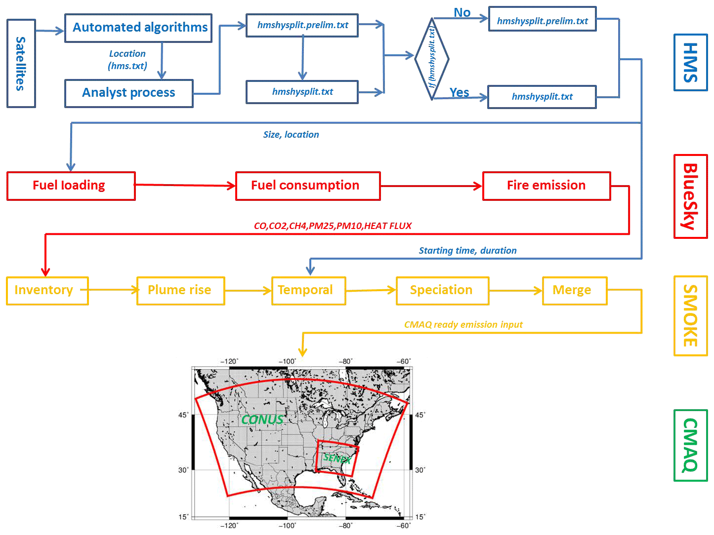
Figure 1Schematics of fire emission and smoke plume simulation system used: data feed and/or modeling of physical and chemical processes were handled largely sequentially from top to bottom and from left to right. The right-hand four vertical boxes depict the submodel names: NESDIS Hazard Mapping System (HMS) for wildfire hotspot detection; the US Forest Service's BlueSky for fuel type and loading parameterization; the US EPA's Sparse Matrix Operator Kernel (SMOKE) for handling emission characterization; and lastly the Community Multiple-scale Air Quality model (CMAQ) for simulating the transformation, transport and depositions of the atmospheric constituents. The “SENEX” inset framed by bold red lines was the domain for this study.
2.1 HMS (Hazard Mapping System)
The NOAA NESDIS HMS is a fire smoke detection system based on satellite retrievals. At the time of this study, the satellite constellation used consists of two versions of the Geostationary Operational Environmental Satellite (GOES-10 and GOES-12) and five polar-orbiting satellites: MODIS (Moderate-resolution Imaging Spectroradiometer) instruments on NASA Earth Orbiting Sysmte (EOS) Terra and Aqua satellites, and AVHRR (Advanced Very High Resolution Radiometer) instruments on NOAA 15, 17 and 18 satellites. HMS detects wildland fire locations and analyzes their sizes, starting times and durations (Ruminski et al., 2008; Schroeder et al., 2008; Ruminski and Kondragunta, 2006).
HMS first processes satellite data by using automated algorithms for each of the satellite platforms to detect fire locations (Justice et al., 2002; Giglio et al., 2003; Prins and Menzel, 1992; Li et al., 2000), which is then manually analyzed by analysts to eliminate false detections and/or add missed fire hotspots. The size of the fire is represented by the number of detecting pixels corresponding to the nominal resolution of MODIS or AVHRR data. Fire starting times and durations are estimated from close inspection of the visible-band satellite imagery. A bookkeeping file is generated at the end of this detection step, named “hms.txt” (Fig. 1). It includes all the thermal signal hotspots detected by the aforementioned seven satellites. During the analyst quality control step, detected potential fire hotspots lacking visible smoke in the retrieval's HMS (RGB real-color) imagery are removed, resulting in a reduced fire hotspot file called either “hmshysplit.prelim.txt” or “hmshysplit.txt” to be input into the BlueSky processing step.
In general, hmshysplit.prelim.txt and hmshysplit.txt are very similar, and hmshysplit.txt is created later than hmshysplit.prelim.txt (Fig. 1). But the differences between hmx.txt and hmshysplit.txt (hmshysplit.prelim.txt) can be rather substantial. The reasons for the differences are that (1) many detected fires do not produce detectable smoke; (2) some fires/hotspots are detected only at night, when smoke detection is not possible; and (3) smoke emission HMS imagery is obscured by clouds and thus not detected by the analyst. Therefore, smoke emission occurrence provided by the HMS is a conservative estimate of fire emissions.
Through use of multiple satellites, the likelihood of detecting fires in HMS is robust. However, when the fire's geographical size is small, the HMS detection accuracy dramatically decreases (Zhang et al., 2011; Hu et al., 2016). Other limitations of the HMS fire detections include ineffective retrievals at nighttime and under cloud cover.
2.2 BlueSky
BlueSky, developed by the USFS, is a modeling framework for simulating smoke impacts on regional air quality (Larkin et al., 2009; Strand et al., 2012). In this study, BlueSky acted as a fire emission model to provide input for SMOKE (Herron-Thorpe et al., 2014; Baker et al., 2016). BlueSky calculates fire emission based on HMS-derived locations (Fig. 1).
Fire's geographical extent is reflected by the number of nearby fire pixels detected by satellites in a 12 km CMAQ model grid. Fire pixels are converted to fire burning areas in BlueSky based on the assumption that each fire pixel has a size of 1 km2 and 10 % of its area can be considered as burn-active (Rolph et al., 2009). All fire pixels in a 12 km grid square are aggregated. BlueSky uses the following to estimate biomass availability: a fuel loading map from the US National Fire Danger Rating System (NFDRS) for the conterminous USA (CONUS) with the exception of the western USA, where the Hardy set is used (Hardy and Hardy, 2007). BlueSky uses the Emissions Production Model (EPM) (Sandberg and Peterson, 1984), a simple version of the CONSUME model (version 3.0, https://www.fs.fed.us/pnw/fera/research/smoke/consume/index.shtml, last access: 6 May 2020), to calculate fuel actually burned – the so-called consumption sums. Finally, EPM is also used in BlueSky to calculate the fire emission hourly rate per grid cell. BlueSky outputs CO, CO2, CH4, non-methane hydrocarbons (NMHC), total particulate matter (PM), PM2.5, PM10 and heat flux (Fig. 1).
BlueSky does not iteratively recalculate fire duration according to the modeled diminishing fuel loading or the modeled fire behavior. In the aggregation process, when there is more than one HMS point in a grid cell which have different durations, all points in that grid cell are assigned the largest duration in all points. For example, if there were three HMS points that had durations of 10, 10 and 24 h, the aggregation would include three points (representing 3 km2) assigned with 24 h duration to all of the three HMS points.
HMS has no information about fuel loading. BlueSky uses a default fuel loading climatology over the eastern USA. BlueSky uses an idealized diurnal profile for fire emissions. Uncertainties in fire sizes, fuel loading and fire emission rates lead to large uncertainties in wildland smoke emissions (Knorr et al., 2012; Drury et al., 2014; Davis et al., 2015).
2.3 SMOKE
In SMOKE (Sparse Matrix Operator Kernel Emission), the BlueSky fire emissions data in a longitude–latitude map projection are converted to CMAQ-ready gridded emission files (Fig. 1). Fire smoke plume rise is calculated using formulas by Briggs (1975). The heat flux from BlueSky and NAM meteorological state variables are used as input (Erbrink, 1994). The Briggs algorithm calculates plume top and plume bottom; between plume top and bottom the emission fraction is calculated layer by layer assuming a linear distribution of flux strength in atmospheric pressure. For model layers below the plume bottom the emission fraction is assumed to be entirely in the smoldering condition as a function of the fire burning area.
A speciation cross-reference map was adopted to match BlueSky chemical species to those in CMAQ using the US EPA Source Classification Codes (SCCs) for forest wildfires (https://ofmpub.epa.gov/sccsearch/docs/SCC-IntroToSCCs.pdf, last access: 30 April 2020). The life span of fire is based on the HMS-detected fire starting time and duration. During fire burning hours a constant emission rate is assumed. This constant burn rate has been shown to be a crude estimate (Saide et al., 2015; Alvarado et al., 2015). Other uncertainties include plume rise (Sofiev et al., 2012; Urbanski et al., 2014; Achtemeier et al., 2011) and fire weather (fire influencing local weather).
2.4 CMAQ
The CMAQ version 4.7.1 was used. The CB05 gas phase chemical mechanism (Yarwood et al., 2005) and the AERO5 aerosol module (Carlton et al., 2010) were chosen. Anthropogenic emissions were based on the US EPA 2005 National Emission Inventory (NEI) projected to 2013 (Pan et al., 2014); biogenic emissions (BEIS 3.14) were calculated in-line inside CMAQ.
2.5 Simulations
The NAM provided meteorology fields to drive CMAQ (Chai et al., 2013). NAM meteorology is evaluated daily and results (bias, root mean square error etc.) are posted at https://www.emc.ncep.noaa.gov/mmb/nammeteograms (last access: 30 April 2020). The simulation domain is shown in Fig. 1. It includes two domains: (i) a 12 km domain covering the CONUS and (ii) a 4 km domain covering the southeastern USA, where the majority of SENEX measurements occurred. Lateral boundary conditions (LBCs) used in the smaller SENEX domain simulation were extracted from that from the CONUS simulations. Four scenarios were simulated: CONUS with fire emissions, CONUS without fire emissions, SENEX with fire emissions and SENEX without fire emissions.
There were several differences in system configuration between the NAQFC fire smoke forecasting and the “with-fire” simulation in this study. For models, the BlueSky versions used in NAQFC and in this study are v3.5.1 and v2.5, respectively; CMAQ versions used in NAQFC and in this study are v5.0.2 and v4.7.1, respectively. For simulations, current fire smoke forecasting in the NAQFC includes two runs: the analysis and the forecast (H. C. Huang et al., 2017). The analytical run is a 24 h retrospective simulation using yesterday's meteorology and fire emissions to provide initial conditions for today's forecast. The forecasting run is a 48 h predictive simulation using yesterday's fire emissions, assuming fires with duration of more than 24 h are projected as continued fires. The with-fire simulation in this study is exactly identical to the analysis run in NAQFC.
2.6 Evaluations
Carbon monoxide (CO) has a relatively long lifetime in the air and is emitted by biomass burning. CO was used as a fire tracer in the prediction. The CO difference (ΔCO) between CMAQ simulations with and without fire emissions was used as the indicator of fire influence. Additional observations included potassium (K) collected at the IMPROVE sites within the SENEX domain, acetonitrile (CH3CN) measured from the SENEX campaign flights and fire plume shape detected by the HMS analysis as real fire signals. The enhancement in ΔCO concentration due to fire was directly compared with those signals. At the same time, ΔAOD (aerosol optical depth) from CMAQ (concentration simulated with fire minus that without fire) was also used as a fire indicator when compared with smoke masks given by the ASDTA.
It is almost impossible to assess the uncertainty of each specific physical process of smoke. In each modeling step in HMS, BlueSky, SMOKE and CMAQ, the modeling system accrues uncertainties. Such uncertainties were likely cumulative and might lead to larger error in succeeding components (Wiedinmyer et al., 2011). For example, heat flux from BlueSky influenced plume rise height in SMOKE and consequently influenced plume transport in CMAQ. It is also noteworthy that when modeled ΔCO was against measured K or CH3CN the objective was to search for enhancement signals resulting from fires but not to account for proportional concentration changes in the tracers in the event of a fire. Attempting to account for CMAQ simulation uncertainties in surface ozone and particulate matter as a function of smoke emissions from fires was difficult, but that was not the objective of this study. Rather, the purpose of this study is to focus on analyzing the capability of the HMS–BlueSky–SMOKE–CMAQ modeling system to capture fire signals.
The SENEX campaign occurred in June and July, and our model simulations were from 10 June to 20 July 2013. Throughout the campaign all available observation data sets were used, including ground-, air- and satellite-based acquired data. Each data set had its unique characteristics, and linking them together gave an overall evaluation. At the same time, in each data set our evaluations included as many observed fire cases as possible. Both well-predicted and poorly predicted cases are presented to illustrate potential reasons for the modeling system's behavior.
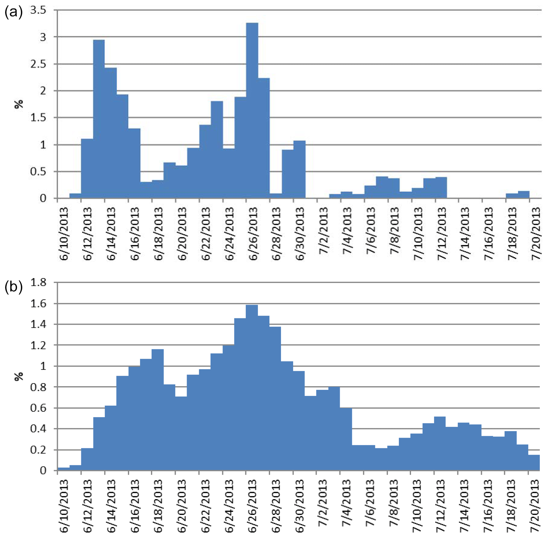
Figure 2In the 4 km SENEX domain, (a) the contribution (%) of CO emission from fires that occurred inside the SENEX domain and (b) the contribution (%) of CO flux flowing into the SENEX domain from its boundary caused by fires burning outside the SENEX domain but inside the CONUS domain.
3.1 Observed CO versus modeled CO in SENEX
Table 1 lists observed and modeled CO vertical profiles for the with-fire and without-fire cases during the SENEX campaign. Observed CO concentrations between the surface and 7 km a.g.l. (above ground level) in the SENEX domain area remained greater than 100 ppb during all 40 d of the campaign. The highest CO concentrations were measured closer to the surface. The maximum measured CO concentration of 1277 ppb was observed during a flight on 3 July at 974 m a.s.l. (above sea level). During this flight strong fire signals were observed, but the fire simulation system missed those signals as discussed below.
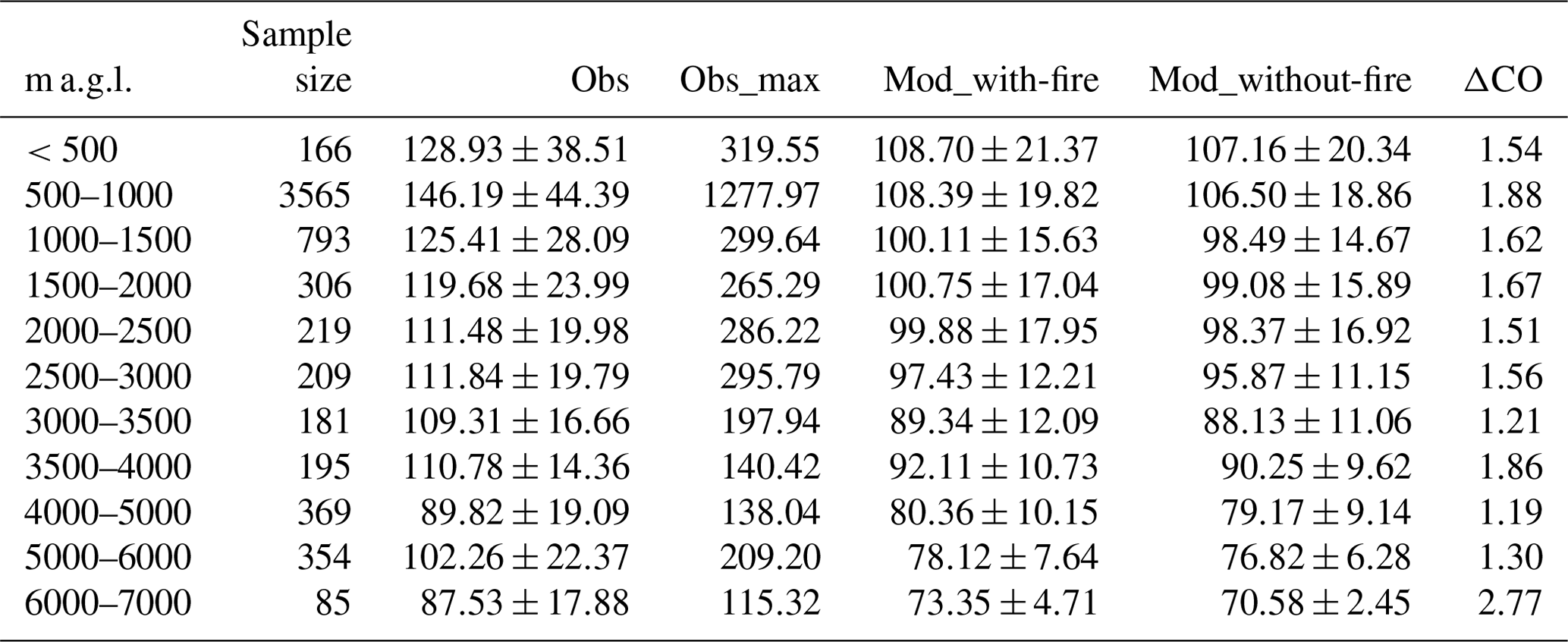
Table 2Identified fire signals from IMPROVE measurements during SENEX.

Notes: (ratios for EC, OC and K>1.2) ∩ (ratio for soil<1.0) ∩ (ratios for and < 1.5).
CO concentrations were underestimated by the model in almost all cases even when the model captured CO contribution from fire emissions spatiotemporally. Mean ΔCO in each height interval was usually above 1.5 ppb but less than 2.0 ppb. Figure 2a shows the contribution of total CO emissions from fires which occurred inside the SENEX domain over the simulation period. The maximum CO emissions contribution from fires was about 3 % during the campaign. On most of those days fire emission contributions in SENEX were less than 1 %. The average contribution during those 40 d was 0.7 %. Figure 2b shows the contribution of CO flowing into the SENEX domain from its boundary caused by fire outside the SENEX domain but inside the CONUS domain (Fig. 1). The average fire contribution to CO from outside the SENEX domain was 0.67 %. CO influenced by fire emission in June is greater than that in July.
During the field experiment the general lack of large fires made evaluation of modeled fire signature difficult since it was easier to capture large fire signals than the smaller fires. We postulated that a clear fire signal simulated in the HMS–BlueSky–SMOKE–CMAQ system could be indicated by ΔCO significantly larger than its temporal averages resulting from fires that originated inside and/or outside the SENEX domain. For example, a clear fire signal between 500 and 1000 m a.g.l. was indicated by the ΔCO concentration that was above 2.0 ppb. It was based on the contributions of fire outside the SENEX domain and inside the SENEX domain to CO and the average CO concentration at these altitudes during SENEX of about 150 ppb ().
Figure 3 displays the simulated ΔCO extracted along the SENEX flight path during the SENEX campaign. The modeled concentration showed that the fire impacts on SENEX were not negligible despite a lack of larger fire events as shown in Fig. 2a and b during the SENEX campaign period. That confirmed the importance of evaluating the fire simulation system in an air quality model. Unless a model is able to predict fire signals correctly, it is useless for modelers to discuss fire effects on chemical composition of the atmosphere. Details on how the model caught, missed or falsely predicted fire signals during the SENEX campaign and a comparison of ΔCO versus CH3CN will be discussed in the following discussion.
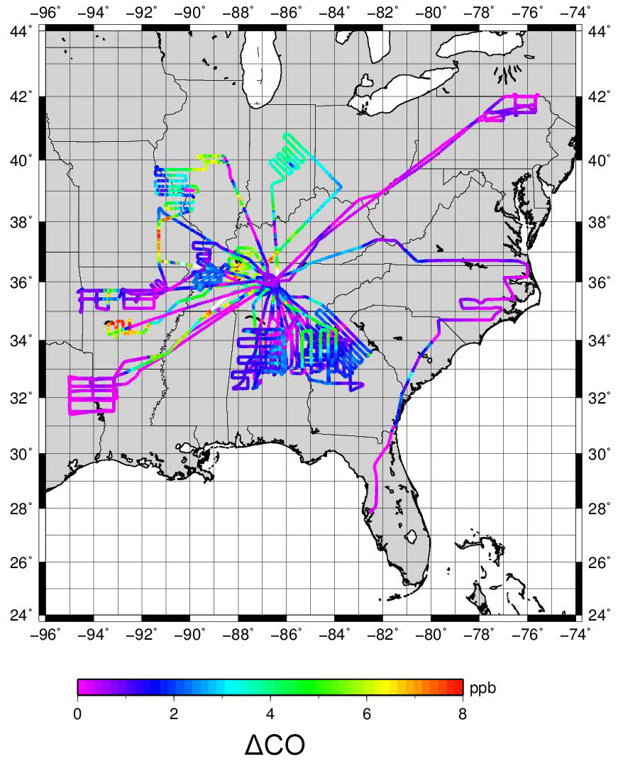
Figure 3CMAQ-simulated ΔCO (ppb), i.e., the CO concentration difference between CMAQ simulation with and without fire emissions, extracted along the overall SENEX flight paths during the SENEX campaign between 10 June and 20 July 2013.
3.2 IMPROVE
The Interagency Monitoring of Protected Visual Environments (IMPROVE) is a long-term air visibility monitoring program initiated in 1985 (http://vista.cira.colostate.edu/Improve/data-page, last access: 30 April 2020). It provides 24 h integrated PM speciation measurements every third day (Malm et al., 2004; Eatough et al., 1996). The IMPROVE data set was chosen for this analysis because it included K (potassium), OC (organic carbon) and EC (elemental carbon), important fire tracers. IMPROVE monitors are ground observation sites likely influenced by nearby fire sources.
There were 14 IMPROVE sites in the SENEX domain (Fig. 4). Potential fire signals were identified using CMAQ-modeled ΔCO and IMPROVE-observed K. However, in addition to fires K has multiple sources such as soil, sea salt and industry. Coincidentally fires should also produce enhanced EC and OC concentrations; a fire signal should reflect above-average values for EC, OC and K. EC, OC and K observations that were 20 % above their temporal averages during the SENEX campaign were used as a predictor for fire event identification. Meanwhile, co-measured (nitrate) and (sulfate) concentrations are less than 1.5 times their respective temporal averages for screening out data with industrial influences. Lastly, a third predictor was employed so that concentrations of other soil components besides K should be below their temporal average to eliminate conditions of spikes in K concentration due to dust. With these three criteria the IMPROVE data were screened for fire events (see Table 2).
Five fire events were observed at four IMPROVE sites. Table 2 lists measured EC, OC, , K, soil and concentrations (µg m−3) and their ratios to averages. BC / OC and K / BC ratios were also calculated and are listed in Table 2 to illustrate the application of our criteria. It was found that, except for monitor BRIS (Breton Island), all other sites (COHU – Cohutta, GA; MACA – Mammoth Cave NP, KY; GRSM – Great Smoky Mountains NP, TN) had BC / OC and K / BC ratios comparable to the ratios of the same quantities due to biomass burning reported by other researchers (Reid et al., 2005; DeBell et al., 2004). BRIS is a coastal site likely influenced by sea salt (Fig. 4).
For the four identified fire cases, ΔCO as a modeled fire tracer around the IMPROVE site was plotted. Fire signals on 21 June at COHU and GRSM and on 24 June at MACA were reproduced in the with-fire model simulation. The 24 June MACA case was used as an example (see Fig. 4). On 24 June 2013, detected fire spots were outside the SENEX domain, but SSW (south-southwest) wind blew smoke plumes into the SENEX domain and affected modeled CO at MACA. Modeled ΔCO at MACA was 5 ppb.
Another IMPROVE site located upwind of MACA, CADI, was also potentially under the influence of that fire event; however, data from CADI on 24 June did not indicate a fire influence, possibly due to the frequency of IMPROVE sampling that eluded measurement or because the smoke plume was transported above the surface in disagreement with what was modeled. Within the four fire cases identified by the IMPROVE data during SENEX (Table 2), the model successfully captured three out of four events. The model missed the fire signal on 3 July at MACA. The following section is dedicated to the 3 July SENEX flight.
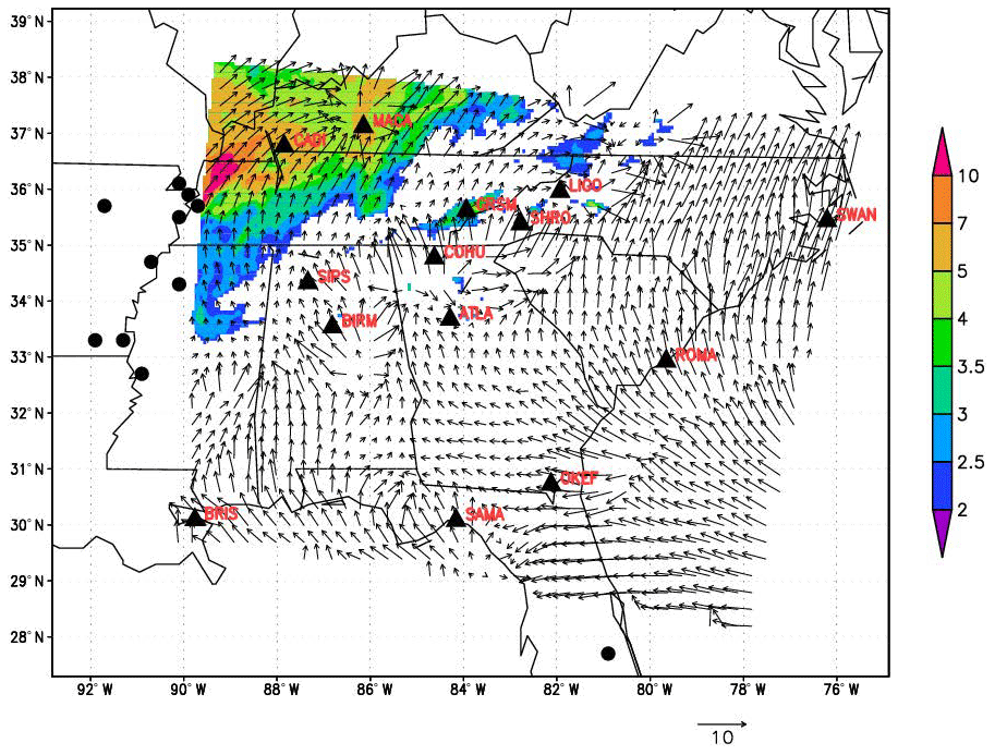
Figure 4Simulated ΔCO (>2.0 ppb) in the SENEX domain on 24 June 2013 at 20:00 UTC overlaid with 2 m wind arrows with a 10 m s−1 reference arrow shown in the bottom right. The solid black circle is detected fire hotspots by HMS. The solid triangles labeled with station code represent IMPROVE sites used in model verification calculations.
3.3 Plume spatial coverage
HMS determines fire hotspot locations associated with smoke and upon incorporating the smoke plume shape information from visible satellite images. HMS provides smoke plume shapefiles over much of North America, which is a two-dimensional smoke plume spatial depiction collapsing all plume stratifications to a satellite's view seen from high above. For modeled plumes, we integrated modeled ΔCO by multiplying the layer values with the corresponding CMAQ model layer thicknesses and air density to derive a simulated smoke plume shape. HMS-derived smoke plume shape versus CMAQ-predicted smoke plume shape was then used to evaluate the fire simulation.
Figure of merits in space (FMS) (Rolph et al., 2009) is a statistic for spatial analysis and was calculated as follows:
where Area_hms represent the area of grid cells influenced by fire emission over CONUS detected by HMS and Area_cmaq represent the area of grid cells over CONUS identified by model prediction. In general, a higher FMS value indicates a better agreement between the observed and modeled plume shape (Rolph et al., 2009).
Figure 5 summarizes FMS during the SENEX campaign. Average FMS was 22 % with its maximum at 56 % on 6 July and minimum at 1.2 % on 17 June 2013. Figure 6a exhibits the HMS-detected smoke plume and CMAQ-calculated smoke plume over CONUS on 6 July. The FMS score was 56 %, meaning that the modeled plume shape was consistent with that of HMS. However, HMS–BlueSky–SMOKE–CMAQ emissions system might have underestimated the intensive fire influence areas along the border of California and Nevada. Subsequently, the model also underpredicted its associated influence in North Dakota, South Dakota, Minnesota, Iowa and Wisconsin.
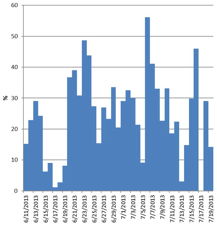
Figure 5FMS (figure of merits in space) (%) from 11 June to 19 July in 2013 during the SENEX campaign.
Figure 6b exhibits the worst case on 17 June 2013 with a FMS score of 1.2 %. There are two reasons for this: (i) CMAQ missed the fire emissions from Canada. Those fire sources were located outside the CONUS modeling domain, and our simulation system used a climatologically based static LBC. Secondly on 17 June, there were a lot of fire hotspots in the southeastern USA, i.e., in Louisiana, Arkansas and Mississippi along the Mississippi River. Hotspots were detected, but they lacked associated smoke in the corresponding HMS imagery (Fig. 6c). This could be due to cloud blockage or to small agricultural debris clearing, burns in underbrush or prescribed burns. These conditions prevented the HMS from identifying fires, and hence emissions were not modeled for those sources.
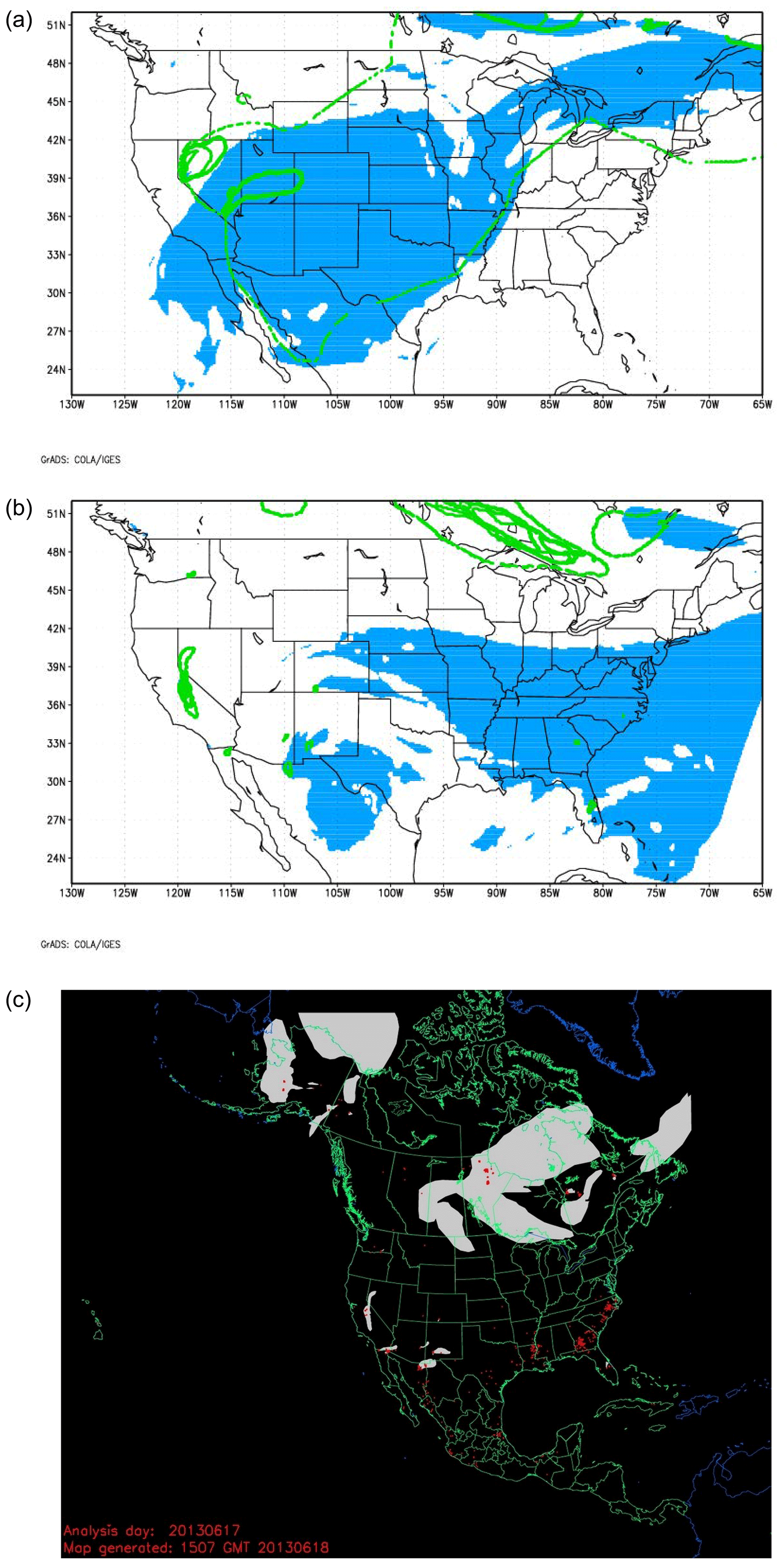
Figure 6Daily HMS-observed plume shape versus CMAQ-predicted daily averaged plume shape on (a) 6 July 2013 and (b) 17 June 2013. The light blue shading represents modeled plume shape (defined as total column ΔCO), and the thin dashed line and bold green lines encircle areas representing HMS-derived lightly and strongly influenced plume shape, respectively. (c) HMS-observed fire hotspots (red) and plume shapes (white) (http://ready.arl.noaa.gov/data/archives/fires/national/arcweb, last access: 30 April 2020) on 17 June 2013.
It is noteworthy that the FMS evaluation contained uncertainties contributed from both modeled and observed values. The calculated campaign duration and SENEX-wide average FMS was 22 %. It is significantly higher than that achieved by similar analyses done by HYSPLIT (Hybrid Single Particle Lagrangian Integrated Trajectory) smoke forecasting for the fire season of 2007 (6.1 to 11.6 %) (Rolph et al., 2009). The primary reason is that due to retrieval latency and cycle-queuing problems in HMS, HMS fire information is delayed by 1 d, which means that today's HMS list can only reflect yesterday's fire information, so HYSPLIT smoke forecasting can only use yesterday's fire information. However, our model simulation in this study was from a retrospective module using current-day fire information. Such discrepancies have been discussed by Huang et al. (2020). The secondary reason is plume rise: although the HYSPLIT and CMAQ fire plume rise were both estimated by the Briggs equation, the HYSPLIT plume rise was limited to 75 % of the mixed layer height (MLH) during daytime and 2 times MLH at nighttime, whereas the CMAQ fire plume rise did not have these limitations.
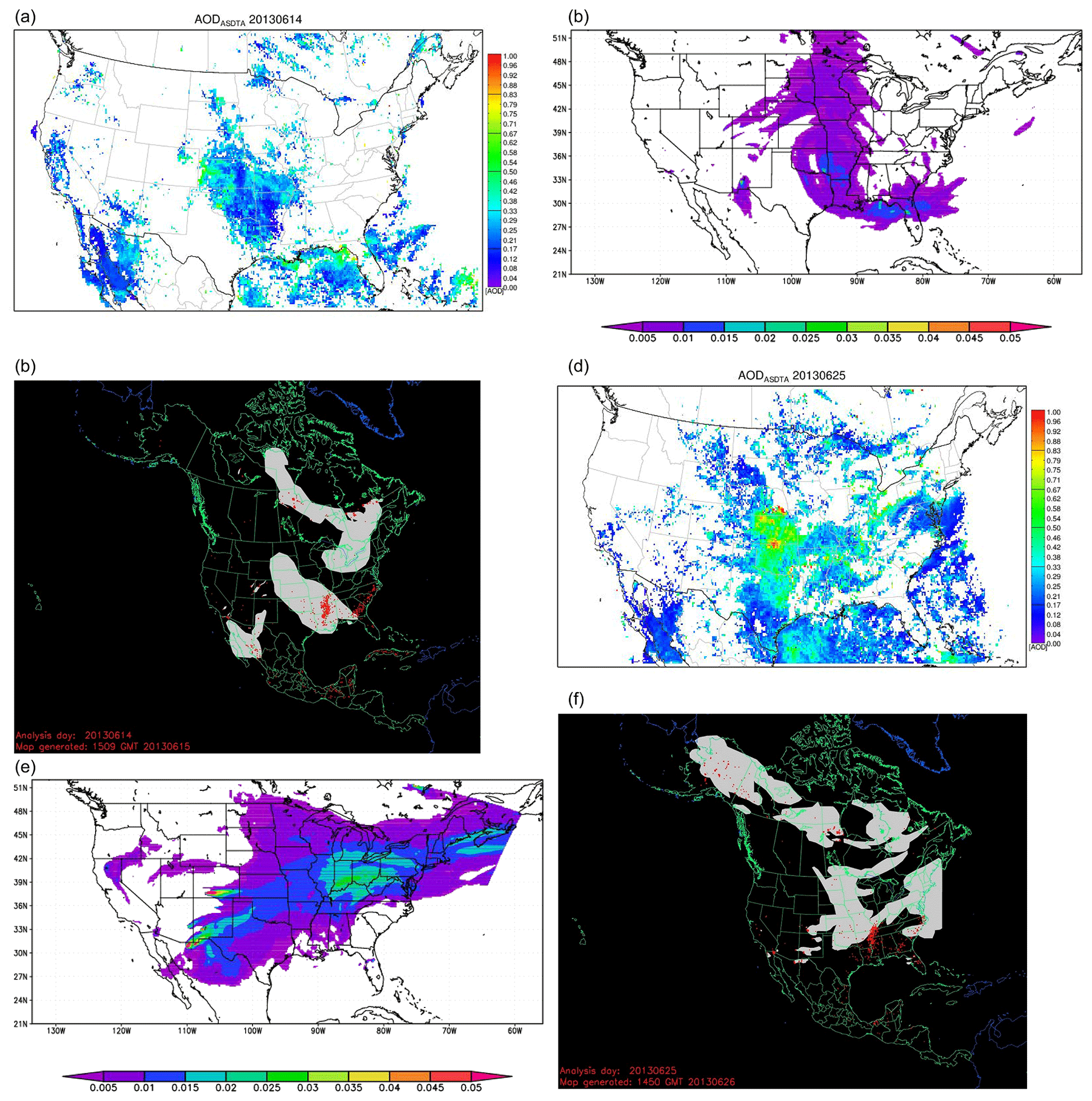
Figure 7GOES-detected AOD influenced by fires using the ASDTA diagnostic method (summed over 10:00 to 14:00 local time). Color-shaded region represents the fire-smoke-influenced areas, and the color denotes the magnitude of the retrieved AOD on (a) 14 June 2013 and (d) 25 June 2013; simulated ΔAOD (with-fire − without-fire) calculated by CMAQ on (b) 14 June 2013 and (e) 25 June 2013; and HMS-observed fire hotspots (red) and plume shapes (white) on (c) 14 June 2013 and (f) 25 June 2013.
3.4 ASDTA
The Automated Smoke Detection and Tracking Algorithm (ASDTA) is a combination of two data sets: (1) the NOAA geostationary satellite (GOES-13), which retrieves thermally enhanced aerosol optical depth due to fires using visible channels and produces a product called GOES Aerosol/Smoke Product (GASP) (Prados et al., 2007), and (2) NOAA NESDIS HMS fire smoke detection. First, the observation of the increase in AOD near the fire is attributed to the specific HMS fire; AOD values not associated with fires are dropped. Second, a pattern recognition scheme uses 30 min geostationary satellite AOD images to track the transport of this smoke plume away from the source. ASDTA provides the capability to determine whether the GASP is influenced by one or multiple smoke plumes over a location at a certain time.
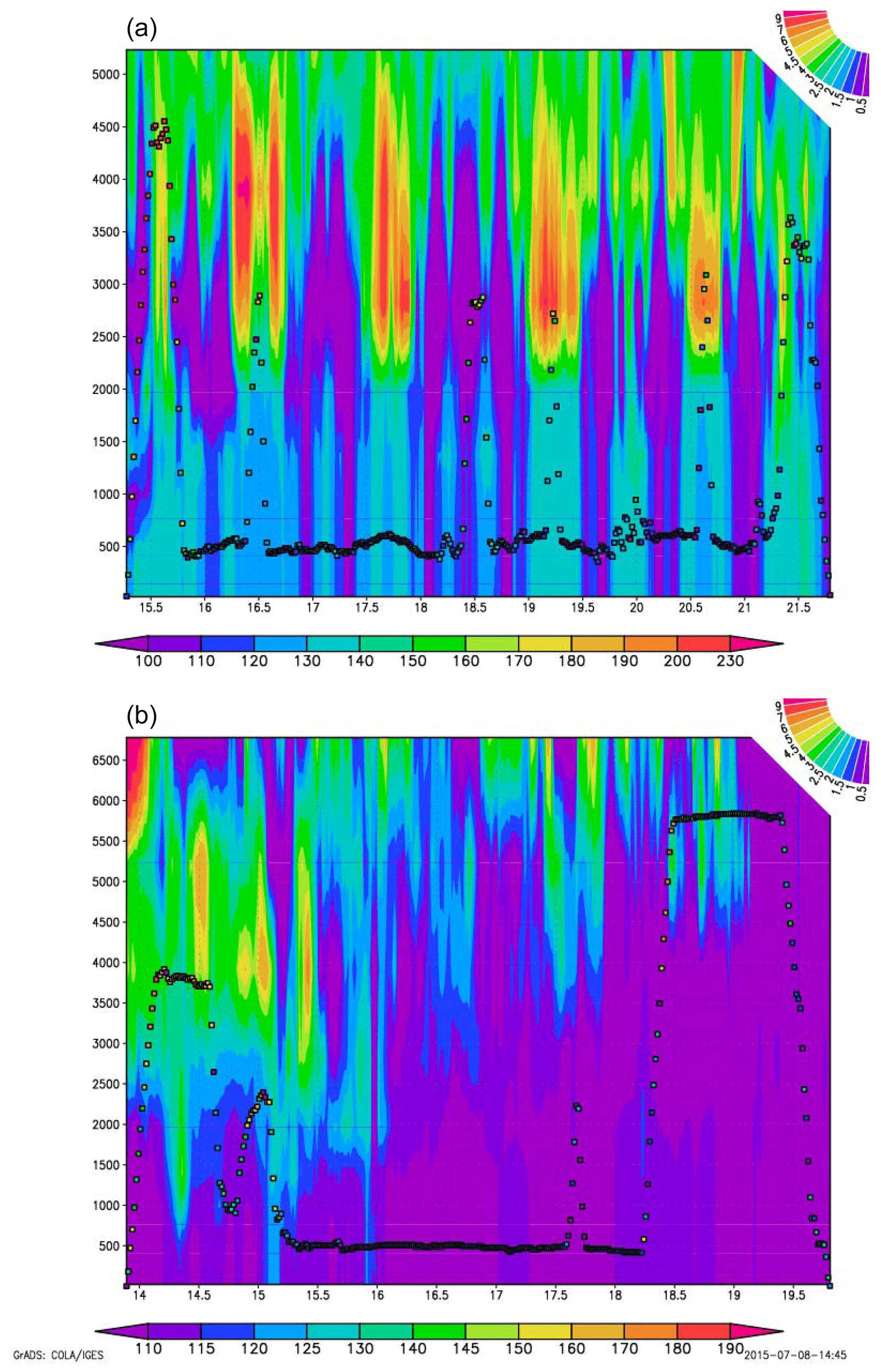
Figure 8Vertical distributions of CMAQ-simulated ΔCO (ppb) shown along a flight transect on (a) 16 June 2013 and (b) 10 July 2013; the x-axis label is UTC (hour) and y-axis label is meters a.g.l. Two color bars represent observed CH3CN concentration (filled square dots and rectangle bar in ppt) and simulated ΔCO concentration (backdrop color shading and fan bar in ppb), respectively.
ASDTA, originally generated to provide operational support for verification of the NOAA HYSPLIT dispersion model, predicts smoke plume direction and extension (Draxler and Hess, 1998). These data are also suitable for model performance evaluation in this study. For each simulation, modeled AOD was calculated for each sensitivity test (with fire or without fire), and ΔAOD is defined as the difference obtained by subtracting AOD_without-fire from AOD_with-fire.
Figure 7a illustrates a GOES-retrieved AOD (summed over 10:00 to 14:00 local time) contour plot that reflects influences by smoke plumes over the CONUS domain on 14 June 2013. Figure 7b presents similar results but for simulated ΔAOD (with-fire − without-fire). For further evaluation of the HMS-detected smoke plume shape, Fig. 7c can be compared with Fig. 7a and b. Figure 7a shows several regions under the influence of fires in California, northwestern Mexico, Kansas, Missouri, Oklahoma, Arkansas, Texas and part of the Gulf of Mexico. In the northeastern USA, fire plumes occurred occasionally. Those regions agreed relatively well with the shaded contours between Fig. 7a and c. However, due to the lack of fire treatments in the CMAQ LBC, the simulation (Fig. 7b) missed smoke influence on the northeast region of the CONUS domain. CMAQ also failed to simulate the fire influences in the southwest region of the domain.
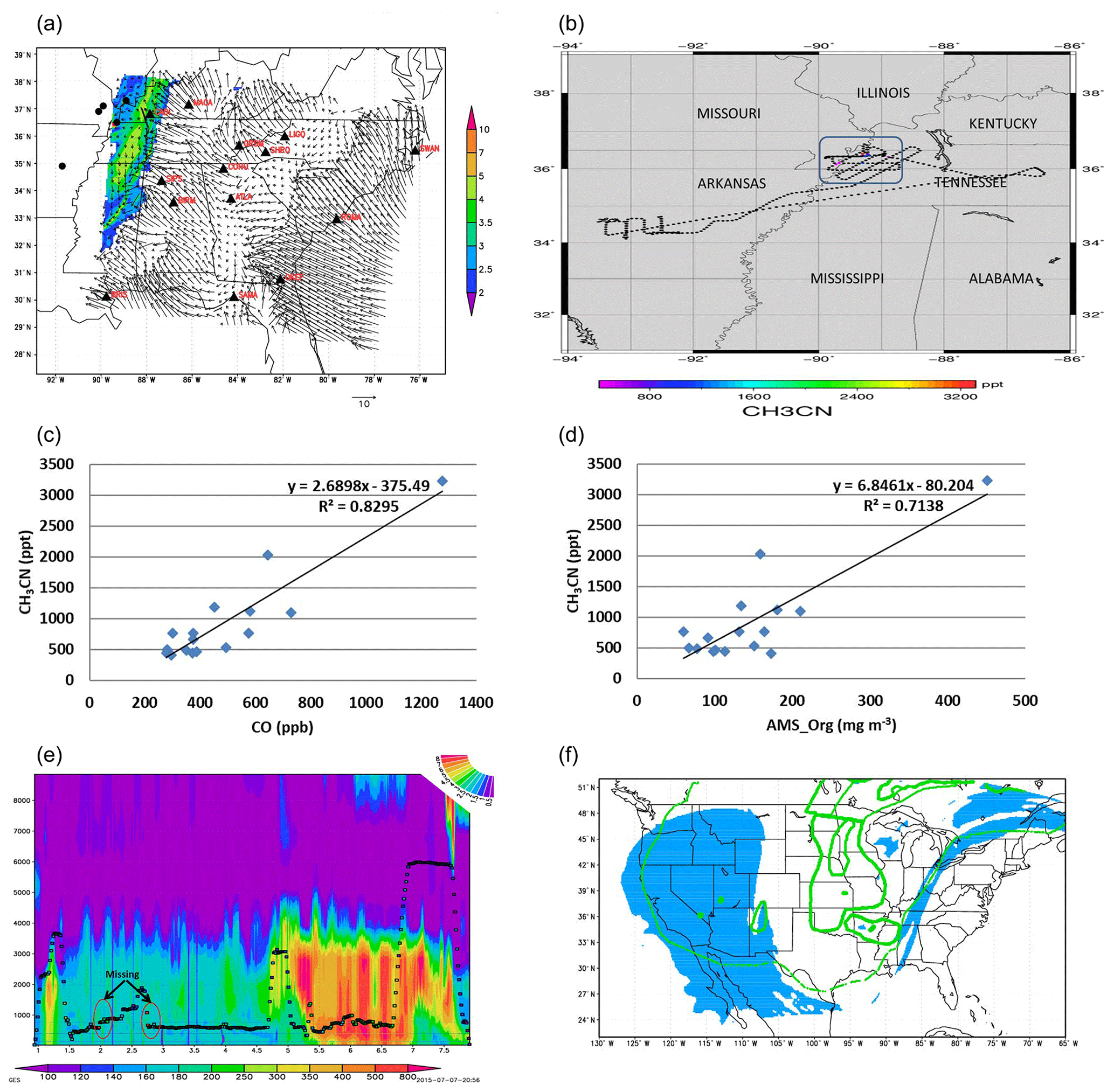
Figure 9Plots for the 3 July 2013 case: (a) IMPROVE, (b) the flight path of SENEX #0703 colored by measured CH3CN concentration (ppt), (c) CH3CN (ppt) vs. CO (ppb), (d) CH3CN (ppt) vs. AMS_Org (mg m−3), (e) CMAQ-simulated ΔCO vertical distributions along a flight transect and (f) HMS-observed plume shape versus CMAQ prediction.
Similar plots for 25 June are shown in Fig. 7d, e and f for ASDTA, CMAQ and HMS, respectively. The ASDTA (Fig. 7d) diagnosed an overestimation in fire influences in the South, including Texas and the Gulf of Mexico, and an underestimation in the northeastern USA. On the other hand, the model predicted two strong fire signals clearly: near the border between Arizona and Mexico, and in Colorado (See Fig. 7e). All the fire-influenced areas in Fig. 7e were seen in the observations by HMS in Fig. 7f.
Comparing ASDTA plots and CMAQ ΔAOD plots (Fig. 7a vs. b; Fig. 7d vs. e), both similarities and differences were found. Similarities were attributable to similar fire accounting and meteorology. Differences were attributable to a number of reasons: HMS contains more fire hotspots than those used by CMAQ due to domain size; only fires inside the CONUS were included in the CMAQ fire simulation, and LBCs did not vary to reproduce impacts of wildfires from outside of the domain.
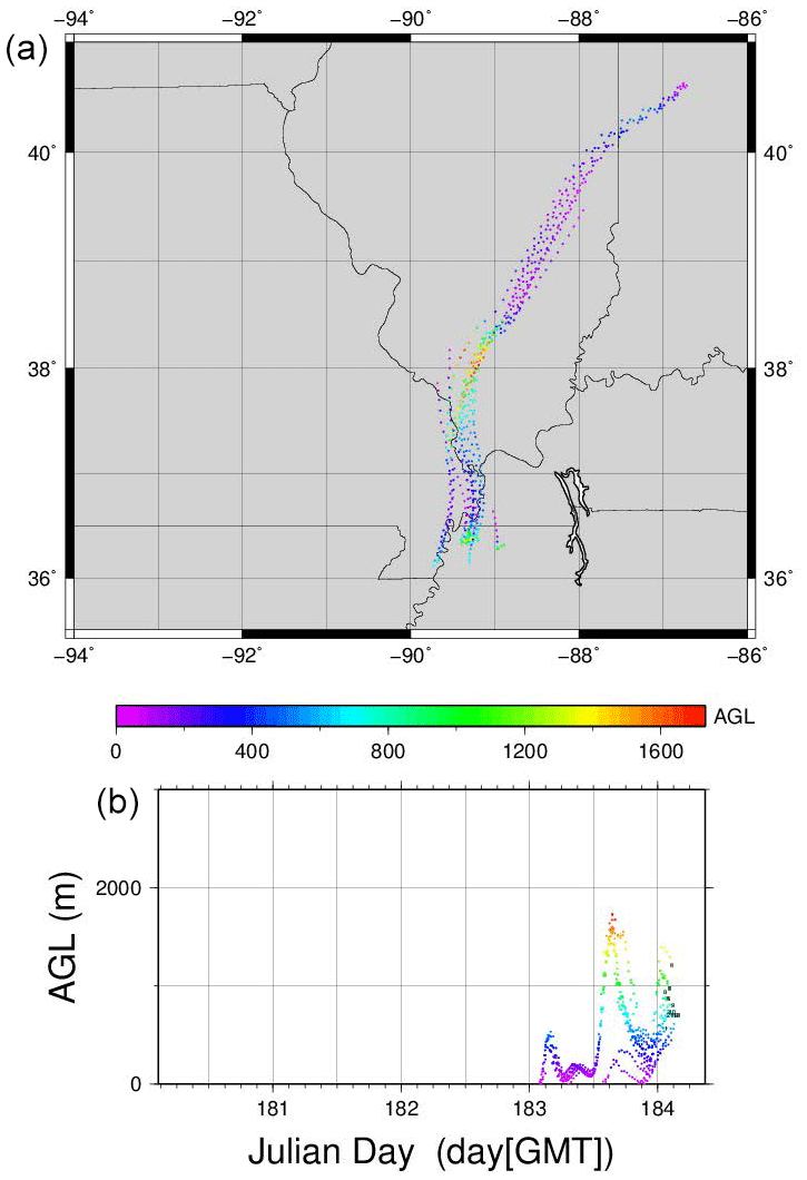
Figure 10A backward-trajectory analysis for CH3CN concentration greater than 400 ppt measured along a SENEX flight on 3 July in (a) aerial and (b) time–vertical cross sections.

Figure 11Detected fire hotspots on 3 July 2013 as daily composite: (a) hmxhysplit.txt and (b) hmx.txt.
3.5 SENEX
SENEX (Southeast Nexus) was a field campaign conducted by NOAA in cooperation with the US EPA and the National Science Foundation in June and July 2013. Although SENEX was not specifically designed for fire studies, its airborne measurements included PM2.5 OC and EC, CO and acetonitrile (CH3CN). CH3CN was chosen as a fire tracer since it is predominantly emitted from biomass burning (Holzinger et al., 1999; Singh et al., 2012).
CH3CN has a residence time in the atmosphere of around 6 months (Hamm and Warneck, 1990), and the reported CH3CN background concentration is around 100–200 ppt (Singh et al., 2003). Measured CH3CN concentrations tend to increase with altitude (Singh et al., 2003; de Gouw et al., 2003), since biomass burning plumes tend to ascend during long-range transport. During SENEX, measured CH3CN showed a similar pattern. Fire signals were identified through airborne measurements of CH3CN when its concentration exceeded the background, e.g., on 3 July 2013, or when its concentration peak appeared at high altitude, e.g., on 16 June 2013 and 10 July 2013.
CH3CN airborne measurements were used to identify fire plumes at certain locations and heights during SENEX. For model evaluation, fire locations and accurate meteorological wind fields are crucial to interpret 2-D measurements such as IMPROVE, HMS and ASDTA. To verify a 3-D fire field, it is critical to capture plume rise. However, it was extremely difficult to figure out plume rise from the airborne measurements. An additional uncertainty arose due to the difference in temporal resolutions of the data: IMPROVE, HMS shapefiles and ASDTA were daily or hourly data, whereas airborne CH3CN data were measured at 1 min intervals.
Figure 8a shows a CMAQ-simulated ΔCO vertical distribution along a flight transect on 16 June 2013. This flight occurred during the weekend over and around power plants around Atlanta, GA. The color along the flight path represents observed CH3CN concentration in ppt. In Fig. 8a, the concentration of ΔCO increased from the surface to 5000 m, especially above 2000 m. Six CH3CN concentration peaks were observed above 2500 m a.g.l.
For CMAQ-simulated ΔCO, five out of six fire signals detected by measured CH3CN spikes were captured where ΔCO concentrations were all above 3 ppb. Only one fire signal was missed by the model at 18:30 UTC on 16 June 2013. The model simulation showed that long-range transport (LRT) of smoke plumes influenced airborne concentrations. Fire signals from the free troposphere subsided and influenced flight measurements. High EC, OC or CO did not concur with the high-CH3CN observation probably due to species lifetime differences. The HMS smoke plume did not show any hotspots or smoke plumes around Atlanta, suggesting that the sources of those observed fire signals were not from its vicinity.
A similar phenomenon was seen on SENEX flight #0710, which occurred during flight transects from Tennessee to Tampa, FL. Figure 8b is a similar graph to Fig. 8a. Based on ΔCO concentrations, CMAQ captured the 10 July case as fire signals were observed. Nonetheless, ΔCO may be overpredicted at around 19:00 UTC. The model exhibited a fire signal with ΔCO concentration of about 3 ppb near 6000 m around 19:00 UTC, whereas measured CH3CN was 120 ppt.
3.6 SENEX flight on 3 July
Observations from IMPROVE, HMS and SENEX identified fire signals on 3 July 2013. ASDTA retrievals were not available. Those signals were missed by the model. In this section, all of the evaluation methods addressed above were used to study potential causes of failure of the model to reproduce the fire signals.
At the MACA IMPROVE site on 3 July 2013, the wind direction at the surface was southeasterly, with no fire hotspots (solid black circle) located upwind of MACA (Fig. 9a). Without any identified hotspots upwind, the model missed fire signals observed at MACA on 3 July 2013.
Flight #0703 was a night mission targeting power plants in Missouri and Arkansas. The flight path is shown in Fig. 9b and is colored by measured CH3CN concentrations. In order to highlight CH3CH concentrations above 400 ppt in the measurements, CH3CN concentrations below 400 ppt were represented by black dots. During the flight, 16 measurements of acetonitrile concentration above 400 ppt were observed, and the maximum was 3227.9 ppt. These observations were located over northwestern Tennessee and close to the borders of Kentucky, Illinois, Missouri and Arkansas. Except for one observation, the flight altitude was between 500 and 1000 m a.s.l.
Enhancements of CO and OC were also measured concurrently with CH3CN. Figure 9c and d show scatter plots for CH3CN versus CO and OC, respectively. Measured CH3CN was highly correlated to both measured CO and OC, with linear correlation coefficients (R2) of 0.83 and 0.71, respectively. The ΔCH3CN / ΔCO ratio is around 2.7 (ppt ppb−1), which is consistent with findings of other measurements over California in 2002 when a strong forest fire signal was intercepted by aircraft (de Gouw et al., 2003). The ΔCH3CN∕ΔOC ratio was around 6.85 (ppt/(mg m−3)), which is also in the range of biomass burning analyses in MILAGRO (Megacity Initiative: Local and Global Research Observations) (Aiken et al., 2010).
Figure 9e shows model-simulated ΔCO with peaks below 3000 m a.g.l. Fire signals have a substantial influences on aircraft measurement at around 05:00 UTC. However, clear fire signals between 02:00 and 03:00 UTC were observed based on prior CH3CN analysis. The model either predicted insufficient fire emission influences or missed it. The FMS score on 3 July was 30 %. Figure 9f shows that CMAQ did not predict plumes where the HMS plume analysis exhibited several dense smoke plumes. As the NOAA Smoke Text Product (http://www.ssd.noaa.gov/PS/FIRE/DATA/SMOKE, last access: 30 April 2020) described in its 3 July 05:01 UTC report, a smaller very dense patch of remnant smoke, analyzed earlier the same day over southern Missouri, drifted southward into Arkansas.
The reasons the model missed these fire observations are not clear. Figures 10, 11a and 11b suggest a few clues. Figure 10 is a backward-trajectory analysis plot for the observations obtained during the SENEX flight on 3 July with observed CH3CN concentrations above 400 ppt. Both transect and passing altitude of the air parcels clearly showed those measurements were most likely influenced by the nearby pollution sources. Figure 11a illustrates the locations of fire used in the CMAQ simulation. It is noted that hmshysplit.txt is input into BlueSky after HMS quality control (Fig. 1). There were several hotspots around the region where the IMPROVE site MACA was located and where the SENEX flight overpassed. Our fire simulation system might have underestimated smoke emissions from those fires. Another explanation can be seen from Fig. 11b, which illustrated hotspots in hmx.txt. In hmx.txt, all fire spots detected by HMS before quality control are shown. Comparing Fig. 11a with b, there are clusters of fire spots in the central USA, especially in western Tennessee. However, those spots were removed during the HMS quality control process because there were no associated smoke plumes visible. In most cases, those fires were believed to be small-sized fires such as from agriculture fires or prescribed burns. For this particular case, there seem to have been thin clouds overhead and thicker clouds in the vicinity (http://inventory.ssec.wisc.edu/inventory/assets/php/image.php?sat=GOES-13&date=2013-7-3&time=16:2&type=Imager&band=1&thefilename=goes13.2013.184.160147.INDX&coverage=CONUS&count=1&offsettz=0, last access: 2 May 2020), so it would be hard to differentiate smoke from clouds by satellite observations.
In support of the NOAA SENEX field experiment in June–July 2013, simulations were conducted including smoke emissions from fires. In this study, a system accounting for fire emissions in a chemical transport model is described, including a satellite fire-detecting system (HMS), a fire emission calculation model (BlueSky), a pre-processing of fire emissions (SMOKE) and simulation over the SENEX domain by CMAQ. The focus of this work is to evaluate the system's capability to capture fire signals identified by multiple observation data sets. These data sets included IMPROVE ground station observations, satellite observations (HMS plume shapefile and ASDTA) and airborne measurements from the SENEX campaign.
For the IMPROVE data, potential fire signals were identified by measured potassium concentrations in PM2.5. Fire identifications in CMAQ rely on predicted ΔCO, the difference between simulations with and without fire emissions. Three out of four observed fire signals were captured by the CMAQ simulations. For HMS smoke plume shapefiles that were manually plotted by analysts to represent the regions impacted by smoke, we used FMS to calculate the percentage of its overlap with CMAQ-predicted smoke plumes. FMS averaged 22 % over 40 days of the SENEX campaign. In terms of fire smoke impacts on ΔAOD, both ASDTA and CMAQ showed patterns that were compared to HMS plume shapefile. In terms of measured CH3CN, a biomass burning plume tracer, both SENEX aircraft in-flight measurements and CMAQ simulations captured signatures of long-range transport of fire emissions from elsewhere in the CONUS domain.
Generally, using HMS-detected fire hotspots and smoke data was useful for predictions of fire impacts and their evaluation. The HMS–BlueSky–SMOKE–CMAQ fire simulation system, which is also used in NAQFC, was able to capture most of the fire signals detected by multiple observations. However, the system failed to identify fire cases on 17 June and 3 July 2013 – thereby demonstrating two problems with the simulation system. One identified problem was the lack of a dynamical fire LBC bounding the CONUS domain to represent the inflow of strong fire signals originating outside the simulation domain. Secondly, the HMS quality control procedure eliminated fire hotspots that were not associated with visible smoke plumes, leading to an underestimation.
We were keen on understanding and quantifying the various uncertainties and observational constraints of this study; therefore the following rules of thumb were observed: (1) a holistic evaluation approach was adopted so that the fire smoke algorithm was interpreted as a single entity to avoid deadlock due to over-interpretation of uncertainty of the single component in the system. (2) An analysis conclusion applicable to the entire simulation period was drawn so that the episodic characteristics of the cases embedded in the simulation were averaged and generalized. This new methodology may benefit NAQFC. (3) We took advantage of the multiple perspectives of the observation systems that offered a wide spectrum of temporal and spatial variabilities intrinsic to the systems; (4) We were intentionally conservative in discarding data so that we maximized the sampling pool for statistical analysis and avoided unwittingly discarding poorly simulated cases, good outliers and weak but accurate signals.
Quantitative evaluation of fire emissions and their subsequent influences on ozone and particulate matter in this fire and smoke prediction system is challenging. Future work includes applying these findings to the NAQFC and improving the NAQFC system's capabilities to simulate fires accurately.
The source code used in this study is available online at https://github.com/NOAA-EMC/EMC_aqfs (last access: 4 May 2020; NOAA-EMC, 2020).
LP, HCK, PL, YHT, DT, BB and JM developed NAQFC fire smoke simulation system. RS, DT, SK, CYX and MGR provided simulation input and observation data. LP, HCK and WWC carried out model simulation and analyzed the result. LP, PL, RS and IS wrote the paper.
The authors declare that they have no conflict of interest.
The authors are thankful to Joost De Gouw and Martin G. Graus of the Earth System Research Laboratory, NOAA, for sharing the SENEX campaign data used in this study. Although this work has been reviewed by the Air Resources Laboratory, NOAA, and approved for publication, it does not necessarily reflect their policies or views.
This research has been supported by the AQAST (grant no. NNH14AX881).
This paper was edited by Fiona O'Connor and reviewed by two anonymous referees.
Achtemeier, G. L., Goodrick, S. A., Liu, Y. Q., Garcia-Menendez, F., Hu, Y. T., and Odman, M. T.: Modeling Smoke Plume-Rise and Dispersion from Southern United States Prescribed Burns with Daysmoke, Atmosphere, 2, 358–388, https://doi.org/10.3390/atmos2030358, 2011.
Aiken, A. C., de Foy, B., Wiedinmyer, C., DeCarlo, P. F., Ulbrich, I. M., Wehrli, M. N., Szidat, S., Prevot, A. S. H., Noda, J., Wacker, L., Volkamer, R., Fortner, E., Wang, J., Laskin, A., Shutthanandan, V., Zheng, J., Zhang, R., Paredes-Miranda, G., Arnott, W. P., Molina, L. T., Sosa, G., Querol, X., and Jimenez, J. L.: Mexico city aerosol analysis during MILAGRO using high resolution aerosol mass spectrometry at the urban supersite (T0) – Part 2: Analysis of the biomass burning contribution and the non-fossil carbon fraction, Atmos. Chem. Phys., 10, 5315–5341, https://doi.org/10.5194/acp-10-5315-2010, 2010.
Alvarado, M. J., Lonsdale, C. R., Yokelson, R. J., Akagi, S. K., Coe, H., Craven, J. S., Fischer, E. V., McMeeking, G. R., Seinfeld, J. H., Soni, T., Taylor, J. W., Weise, D. R., and Wold, C. E.: Investigating the links between ozone and organic aerosol chemistry in a biomass burning plume from a prescribed fire in California chaparral, Atmos. Chem. Phys., 15, 6667–6688, https://doi.org/10.5194/acp-15-6667-2015, 2015.
Baker, K. R., Woody, M. C., Tonnesen, G. S., Hutzell, W., Pye, H. O. T., Beaver, M. R., Pouliot, G., and Pierce, T.: Contribution of regional-scale fire events to ozone and PM2.5 air quality estimated by photochemical modeling approaches, Atmos. Environ., 140, 539–554, https://doi.org/10.1016/j.atmosenv.2016.06.032, 2016.
Briggs, G. A.: Plume rise predictions, in: Lectures on air pollution and environmental impact analyses, Boston, 59–111, 1975.
Carlton, A. G., Bhave, P. V., Napelenok, S. L., Edney, E. D., Sarwar, G., Pinder,R. W., Pouliot, G. A., and Houyoux, M.: Model Representation of Secondary Organic Aerosol in CMAQv4.7, Environ. Sci. Technol., 44, 8553–8560, https://doi.org/10.1021/es100636q, 2010.
Chai, T., Kim, H.-C., Lee, P., Tong, D., Pan, L., Tang, Y., Huang, J., McQueen, J., Tsidulko, M., and Stajner, I.: Evaluation of the United States National Air Quality Forecast Capability experimental real-time predictions in 2010 using Air Quality System ozone and NO2 measurements, Geosci. Model Dev., 6, 1831–1850, https://doi.org/10.5194/gmd-6-1831-2013, 2013.
Davis, A. Y., Ottmar, R., Liu, Y. Q., Goodrick, S., Achtemeier, G., Gullett, B., Aurell, J., Stevens, W., Greenwald, R., Hu, Y. T., Russell, A., Hiers, J. K., and Odman, M. T.: Fire emission uncertainties and their effect on smoke dispersion predictions: a case study at Eglin Air Force Base, Florida, USA, Int. J. Wildl. Fire, 24, 276–285, https://doi.org/10.1071/wf13071, 2015.
DeBell, L. J., Talbot, R. W., Dibb, J. E., Munger, J. W., Fischer, E. V., and Frolking, S. E.: A major regional air pollution event in the northeastern United States caused by extensive forest fires in Quebec, Canada, J. Geophys. Res.-Atmos., 109, D19, https://doi.org/10.1029/2004jd004840, 2004.
de Gouw, J. A., Warneke, C., Parrish, D. D., Holloway, J. S., Trainer, M., and Fehsenfeld, F. C.: Emission sources and ocean uptake of acetonitrile (CH3CN) in the atmosphere, J. Geophys. Res.-Atmos., 108, D11, https://doi.org/10.1029/2002jd002897, 2003.
Delfino, R. J., Brummel, S., Wu, J., Stern, H., Ostro, B., Lipsett, M., Winer, A., Street, D. H., Zhang, L., Tjoa, T., and Gillen, D. L.; The relationship of respiratory and cardiovascular hospital admissions to the southern California wildfires of 2003, Occup. Environm. Med., 66, 189–197, https://doi.org/10.1136/oem.2008.041376, 2009.
Draxler, R. R. and Hess, G. D.: An overview of the HYSPLIT_4 modelling system for trajectories, dispersion and deposition, Aust. Meteorol. Mag., 47, 295–308, 1998.
Dreessen, J., Sullivan, J., and Delgado, R.: Observations and impacts of transported Canadian wildfire smoke on ozone and aerosol air quality in the Maryland region on June 9–12, 2015, J. Air Waste Manage. Assoc., 66, 842–862, https://doi.org/10.1080/10962247.2016.1161674, 2016.
Drury, S. A., Larkin, N., Strand, T. T., Huang, S. M., Strenfel, S. J., Banwell, E. M., O'Brien, T. E., and Raffuse, S. M.: Intercomparison of fire size, fuel loading, fuel consumption, and smoke emissions estimates on the 2006 Tripod Fire, Washington, USA, Fire Ecol., 10, 56–83, https://doi.org/10.4996/fireecology.1001056, 2014.
Eatough, D. J., Eatough, D. A., Lewis, L., and Lewis, E. A.: Fine particulate chemical composition and light extinction at Canyonlands National Park using organic particulate material concentrations obtained with a multisystem, multichannel diffusion denuder sampler, J. Geophys. Res.-Atmos., 101, 19515–19531, https://doi.org/10.1029/95jd01385, 1996.
Erbrink, H. J.: Plume rise in different atmospheres – a practical scheme and some comparisons with lidar measurements, Atmos. Environ., 28, 3625–36336, https://doi.org/10.1016/1352-2310(94)00197-s, 1994.
Giglio, L., Descloitres, J., Justice, C. O., and Kaufman, Y. J.: An enhanced contextual fire detection algorithm for MODIS, Remote Sens. Environ., 87, 273–282, https://doi.org/10.1016/s0034-4257(03)00184-6, 2003.
Hamm, S. and Warneck, P.: The interhemispheric distribution and the budget of acetonitrile in the troposphere, J. Geophys. Res.-Atmos., 95, 20593–20606, https://doi.org/10.1029/JD095iD12p20593, 1990.
Hardy, C. C. and Hardy, C. E.: Fire danger rating in the United States of America: an evolution since 1916, Int. J. Wildl. Fire, 16, 217–231, https://doi.org/10.1071/wf06076, 2007.
Herron-Thorpe, F. L., Mount, G. H., Emmons, L. K., Lamb, B. K., Jaffe, D. A., Wigder, N. L., Chung, S. H., Zhang, R., Woelfle, M. D., and Vaughan, J. K.: Air quality simulations of wildfires in the Pacific Northwest evaluated with surface and satellite observations during the summers of 2007 and 2008, Atmos. Chem. Phys., 14, 12533–12551, https://doi.org/10.5194/acp-14-12533-2014, 2014
Holzinger, R., Warneke, C., Hansel, A., Jordan, A., Lindinger, W., Scharffe, D. H., Schade, G., and Crutzen, P. J.: Biomass burning as a source of formaldehyde, acetaldehyde, methanol, acetone, acetonitrile, and hydrogen cyanide, Geophys. Res. Lett., 26, 1161–1164. https://doi.org/10.1029/1999gl900156, 1999.
Hu, X. F., Yu, C., Tian, D., Ruminski, M., Robertson, K., Waller, L. A., and Liu, Y.: Comparison of the Hazard Mapping System (HMS) fire product to ground-based fire records in Georgia, USA, J. Geophys. Res.-Atmos., 121, 2901–2910, https://doi.org/10.1002/2015jd024448, 2016.
Huang, J., McQueen, J., Wilczak, J., Djalalova, I., Stajner, I., Shafran, P., Allured, D., Lee, P., Pan, L., Tong, D., Huang, H., DiMego, G., Upadhayay, S., and Monache, L.: Improving NOAA NAQFC PM2.5 predictions with a bias correction approach, Weather Forecast., 32, 407–421, https://doi.org/10.1175/WAF-D-16-0118.1, 2017.
Huang, H. C., Pan, L., McQueen, J., Lee, P., ONeill, S. M., Ruminski, M., Shafran, P., Huang, J., Stajner, I., Upadhayay, S., and Larkin, N. K.: The Simulations of Wildland Fire Smoke PM25 in the NWS Air Quality Forecasting Systems, in: AGU Fall Meeting Abstracts, 2017.
Jaffe, D. A., Wigder, N., Downey, N., Pfister, G., Boynard, A., and Reid, S. B.: Impact of Wildfires on Ozone Exceptional Events in the Western US, Environ. Sci. Technol., 47, 11065–11072, https://doi.org/10.1021/es402164f, 2013.
Johnston, F. H., Henderson, S. B., Chen, Y., Randerson, J. T., Marlier, M., DeFries, R. S., Kinney, P., Bowman, D., and Brauer, M.: Estimated Global Mortality Attributable to Smoke from Landscape Fires, Environ. Health Perspect., 120, 695–701, https://doi.org/10.1289/ehp.1104422, 2012.
Justice, C. O., Giglio, L., Korontzi, S., Owens, J., Morisette, J. T., Roy, D., Descloitres, J., Alleaume, S., Petitcolin, F., and Kaufman, Y.: The MODIS fire products, Remote Sens. Environ., 83, 244–262, https://doi.org/10.1016/s0034-4257(02)00076-7, 2002.
Knorr, W., Lehsten, V., and Arneth, A.: Determinants and predictability of global wildfire emissions, Atmos. Chem. Phys., 12, 6845–6861, https://doi.org/10.5194/acp-12-6845-2012, 2012.
Larkin, N. K., O'Neill, S. M., Solomon, R., Raffuse, S., Strand, T., Sullivan, D. C., Krull, C., Rorig, M., Peterson, J. T., and Ferguson, S. A.: The BlueSky smoke modeling framework, Int. J. Wildl. Fire, 18, 906–920, https://doi.org/10.1071/wf07086, 2009.
Li, Z., Nadon, S., and Cihlar, J.: Satellite-based detection of Canadian boreal forest fires: development and application of the algorithm, Int. J. Remote Sens., 21, 3057–3069, https://doi.org/10.1080/01431160050144956, 2000.
Malm, W. C., Schichtel, B. A., Pitchford, M. L., Ashbaugh, L. L., and Eldred, R. A.: Spatial and monthly trends in speciated fine particle concentration in the United States, J. Geophys. Res.-Atmos., 109, D3, https://doi.org/10.1029/2003jd003739, 2004.
Neuman, J. A., Trainer, M., Brown, S. S., Min, K. E., Nowak, J. B., Parrish, D. D., Peischl, J., Pollack, I. B., Roberts, J. M., Ryerson, T. B., and Veres, P. R.: HONO emission and production determined from airborne measurements over the Southeast US, J. Geophys. Res.-Atmos., 121, 9237–9250, https://doi.org/10.1002/2016jd025197, 2016.
NOAA-EMC: EMC-aqfs, GitHub, available at: https://github.com/NOAA-EMC/EMC_aqfs, last access: 4 May 2020.
Pan, L., Tong, D., Lee, P., Kim, H. C., and Chai, T. F.: Assessment of NOx and O3 forecasting performances in the US National Air Quality Forecasting Capability before and after the 2012 major emissions updates, Atmos. Environ., 95, 610–619, https://doi.org/10.1016/j.atmosenv.2014.06.020, 2014.
Pavlovic, R., Chen, J., Anderson, K., Moran, M. D., Beaulieu, P. A., Davignon, D., and Cousineau, S.: The FireWork air quality forecast system with near-real-time biomass burning emissions: Recent developments and evaluation of performance for the 2015 North American wildfire season, J. Air Waste Manage. Assoc., 66, 819–841, https://doi.org/10.1080/10962247.2016.1158214, 2016.
Pius, L., McQueen, J., Stajner, I., Huang, J., Pan, L., Tong, D., Kim, H., Tang, Y., Kondragunta, S., and Ruminski, M.: NAQFC developmental forecast guidance for fine particulate matter (PM2.5), Weather Forecast., 32, 343–360, https://doi.org/10.1175/waf-d-15-0163.1, 2017.
Prados, A. I., Kondragunta, S., Ciren, P., and Knapp, K. P.: GOES Aerosol/Smoke product (GASP) over North America: Comparisons to AERONET and MODIS observations, J. Geophys. Res.-Atmos., 112, D15, https://doi.org/10.1029/2006jd007968, 2007.
Prins, E. M. and Menzel, W. P.: Geostationary satellite detection of biomass burning in South America, Int. J. Remote Sens., 13, 2783–2799, 1992.
Rappold, A. G., Stone, S. L., Cascio, W. E., Neas, L. M., Kilaru, V. J., Carraway, M. S., Szykman, J. J., Ising, A., Cleve, W. E., Meredith, J. T., Vaughan-Batten, H., Deyneka, L., and Devlin, R. B.: Peat Bog Wildfire Smoke Exposure in Rural North Carolina Is Associated with Cardiopulmonary Emergency Department Visits Assessed through Syndromic Surveillance, Environ. Health Perspect., 119, 1415–1420, https://doi.org/10.1289/ehp.1003206, 2011.
Reid, J. S., Koppmann, R., Eck, T. F., and Eleuterio, D. P.: A review of biomass burning emissions part II: intensive physical properties of biomass burning particles, Atmos. Chem. Phys., 5, 799–825, https://doi.org/10.5194/acp-5-799-2005, 2005.
Rolph, G. D., Draxler, R. R., Stein, A. F., Taylor, A., Ruminski, M. G., Kondragunta, S., Zeng, J., Huang, H. C., Manikin, G., McQueen, J. T., and Davidson, P. M.: Description and Verification of the NOAA Smoke Forecasting System: The 2007 Fire Season, Weather Forecast., 24, 361–378. https://doi.org/10.1175/2008waf2222165.1, 2009.
Ruminski, M. and Kondragunta, S.: Monitoring fire and smoke emissions with the hazard mapping system – art. no. 64120B. in: Disaster Forewarning Diagnostic Methods and Management, edited by: Kogan, F., Habib, S., Hegde, V. S., and Matsuoka, M., 2006.
Ruminski, M., Simko, J., Kibler, J., Kondragunta, S., Draxler, R., Davidson, P., and Li, P.: Use of multiple satellite sensors in NOAA's operational near real-time fire and smoke detection and characterization program, in: Remote Sensing of Fire: Science and Application, edited by: Hao, W. M., 2008.
Saide, P. E., Peterson, D. A., da Silva, A., Anderson, B., Ziemba, L. D., Diskin, G., Sachse, G., Hair, J., Butler, C., Fenn, M., Jimenez, J. L., Campuzano-Jost, P., Perring, A. E., Schwarz, J. P., Markovic, M. Z., Russell, P., Redemann, J., Shinozuka, Y., Streets, D. G., Yan, F., Dibb, J., Yokelson, R., Toon, O. B., Hyer, E., and Carmichael, G. R.: Revealing important nocturnal and day-to-day variations in fire smoke emissions through a multiplatform inversion, Geophys. Res. Lett., 42, 3609–3018, https://doi.org/10.1002/2015gl063737, 2015.
Sandberg, D. V. and Peterson, J.: A source strength model for prescribed fires in coniferous logging slash, 1984 annual meeting, Air Pollution Control Association, Northwest Section, 14 p., 1984.
Sapkota, A., Symons, J. M., Kleissl, J., Wang, L., Parlange, M. B., Ondov, J., Breysse, P. N., Diette, G. B., Eggleston, P. A., and Buckley, T. J.: Impact of the 2002 Canadian forest fires on particulate matter air quality in Baltimore City, Environ. Sci. Technol., 39, 24–32, https://doi.org/10.1021/es035311z, 2005.
Schroeder, W., Ruminski, M., Csiszar, I., Giglio, L., Prins, E., Schmidt, C., and Morisette, J.: Validation analyses of an operational fire monitoring product: The Hazard Mapping System, Int. J. Remote Sens., 29, 6059–6066, https://doi.org/10.1080/01431160802235845, 2008.
Singh, H. B., Salas, L., Herlth, D., Kolyer, R., Czech, E., Viezee, W., Li, Q., Jacob, D. J., Blake, D., Sachse, G., Harward, C. N., Fuelberg, H., Kiley, C. M., Zhao, Y., and Kondo, Y.: In situ measurements of HCN and CH3CN over the Pacific Ocean: Sources, sinks, and budgets, J. Geophys. Res.-Atmos., 108, D20, https://doi.org/10.1029/2002jd003006, 2003.
Singh, H. B., Cai, C., Kaduwela, A., Weinheimer, A., and Wisthaler, A.: Interactions of fire emissions and urban pollution over California: Ozone formation and air quality simulations, Atmos. Environ., 56, 45–51, https://doi.org/10.1016/j.atmosenv.2012.03.046, 2012.
Sofiev, M., Ermakova, T., and Vankevich, R.: Evaluation of the smoke-injection height from wild-land fires using remote-sensing data, Atmos. Chem. Phys., 12, 1995–2006, https://doi.org/10.5194/acp-12-1995-2012, 2012.
Strand, T. M., Larkin, N., Craig, K. J., Raffuse, S., Sullivan, D., Solomon, R., Rorig, M., Wheeler, N., and Pryden, D.: Analyses of BlueSky Gateway PM2.5 predictions during the 2007 southern and 2008 northern California fires, J. Geophys. Res.-Atmos., 117, D17, https://doi.org/10.1029/2012jd017627, 2012.
Urbanski, S., Kovalev, V., Petkov, A., Scalise, A., Wold, C., and Hao, W. M.: Validation of smoke plume rise models using ground-based lidar, in: Remote Sensing for Agriculture, Ecosystems, and Hydrology Xvi, edited by: Neale, C. M. U. and Maltese, A., 2014.
Warneke, C., Trainer, M., de Gouw, J. A., Parrish, D. D., Fahey, D. W., Ravishankara, A. R., Middlebrook, A. M., Brock, C. A., Roberts, J. M., Brown, S. S., Neuman, J. A., Lerner, B. M., Lack, D., Law, D., Hübler, G., Pollack, I., Sjostedt, S., Ryerson, T. B., Gilman, J. B., Liao, J., Holloway, J., Peischl, J., Nowak, J. B., Aikin, K. C., Min, K.-E., Washenfelder, R. A., Graus, M. G., Richardson, M., Markovic, M. Z., Wagner, N. L., Welti, A., Veres, P. R., Edwards, P., Schwarz, J. P., Gordon, T., Dube, W. P., McKeen, S. A., Brioude, J., Ahmadov, R., Bougiatioti, A., Lin, J. J., Nenes, A., Wolfe, G. M., Hanisco, T. F., Lee, B. H., Lopez-Hilfiker, F. D., Thornton, J. A., Keutsch, F. N., Kaiser, J., Mao, J., and Hatch, C. D.: Instrumentation and measurement strategy for the NOAA SENEX aircraft campaign as part of the Southeast Atmosphere Study 2013, Atmos. Meas. Tech., 9, 3063–3093, https://doi.org/10.5194/amt-9-3063-2016, 2016.
Wiedinmyer, C., Quayle, B., Geron, C., Belote, A., McKenzie, D., Zhang, X. Y., O'Neill, S., and Wynne, K. K.: Estimating emissions from fires in North America for air quality modeling, Atmos. Environ., 40, 3419–3432, https://doi.org/10.1016/j.atmosenv.2006.02.010, 2006.
Wiedinmyer, C., Akagi, S. K., Yokelson, R. J., Emmons, L. K., Al-Saadi, J. A., Orlando, J. J., and Soja, A. J.: The Fire INventory from NCAR (FINN): a high resolution global model to estimate the emissions from open burning, Geosci. Model Dev., 4, 625–641, https://doi.org/10.5194/gmd-4-625-2011, 2011.
Wotawa, G. and Trainer, M.: The influence of Canadian forest fires on pollutant concentrations in the United States, Science, 288, 324–328, https://doi.org/10.1126/science.288.5464.324, 2000.
Xu, L., Middlebrook, A. M., Liao, J., de Gouw, J. A., Guo, H. Y., Weber, R. J., Nenes, A., Lopez-Hilfiker, F. D., Lee, B. H., Thornton, J. A., Brock, C. A., Neuman, J. A., Nowak, J. B., Pollack, I. B., Welti, A., Graus, M., Warneke, C., and Ng, N. L.: Enhanced formation of isoprene-derived organic aerosol in sulfur-rich power plant plumes during Southeast Nexus, J. Geophys. Res.-Atmos., 121, 11137–11153, https://doi.org/10.1002/2016jd025156, 2016.
Yarwood, G., Rao, S., Yocke, M., and Whitten, G.: Updates to the Carbon Bond Chemical Mechanism: CB05, Technical Report RT-0400675 ENVIRON International Corporation Novato, CA, USA, 2005.
Zhang, X. Y., Kondragunta, S., and Quayle, B.: Estimation of Biomass Burned Areas Using Multiple-Satellite-Observed Active Fires, IEEE Trans. Geosci. Remote Sens., 49, 4469–4482, https://doi.org/10.1109/tgrs.2011.2149535, 2011.