the Creative Commons Attribution 4.0 License.
the Creative Commons Attribution 4.0 License.
 | 22 Apr 2020
Tracking water masses using passive-tracer transport in NEMO v3.4 with NEMOTAM: application to North Atlantic Deep Water and North Atlantic Subtropical Mode Water
Dafydd Stephenson
Simon A. Müller
Florian Sévellec
Water mass ventilation provides an important link between the atmosphere and the global ocean circulation. In this study, we present a newly developed, probabilistic tool for offline water mass tracking. In particular, NEMOTAM, the tangent-linear and adjoint counterpart to the NEMO ocean general circulation model, is modified to allow passive-tracer transport. By terminating dynamic feedbacks in NEMOTAM, tagged water can be tracked forward and backward in time as a passive dye, producing a probability distribution of pathways and origins, respectively. To represent surface (re-)ventilation, we optionally decrease the tracer concentration in the surface layer and track this concentration removal to produce a ventilation record.
Two test cases are detailed, examining the creation and fate of North Atlantic Subtropical Mode Water (NASMW) and North Atlantic Deep Water (NADW) in a 2∘ configuration of NEMO run with repeated annual forcing for up to 400 years. Model NASMW is shown to have an expected age of 4.5 years and is predominantly eradicated by internal processes. A bed of more persistent NASMW is detected below the mixed layer with an expected age of 8.7 years. It is shown that while model NADW has two distinct outcrops (in the Arctic and North Atlantic), its formation primarily takes place in the subpolar Labrador and Irminger seas. Its expected age is 112 years.
- Article
(14211 KB) - Full-text XML
- BibTeX
- EndNote


The intricate process by which the atmosphere and ocean exchange properties has decisive effects on oceanic and atmospheric circulation, biochemistry, and climate. Tracing the pathways of newly ventilated ocean water masses is a multidisciplinary pursuit, for which an entire toolbox of methods has been developed.
Thermocline ventilation and water mass formation is an area with a long history of inquiry. From charts of hydrographic sections, Iselin (1939) inferred communication between isopycnals at depth and their outcrops. This idea was developed theoretically over the following decades in analytical models (Welander, 1959, 1971; Luyten et al., 1983). In this vertically discretised, laminar framework, potential vorticity (PV) conservation facilitates a bijective relationship between the origin and destination of a water parcel. In reality, however, turbulent mixing means that surface-to-deep pathways have a pronounced probabilistic character.
Observational studies have been able to capture snapshots of this turbulent behaviour locally in passive-tracer dye-release experiments (e.g. Schuert, 1970). However, the effect of turbulence on water mass pathways has only been observed on a large scale since the widespread adoption of cost-effective Lagrangian profiling floats, which have been observed to follow chaotic trajectories (e.g. Fischer and Schott, 2002; Fratantoni et al., 2013; Bower et al., 2019). Despite their number (typically several tens of floats for dedicated pathway tracking studies), these trajectories remain undersampled.
Simulations of larger numbers of Lagrangian particles in sophisticated eddy-resolving ocean general circulation models (OGCMs; e.g. Blanke and Raynaud, 1997; Gary et al., 2014) are reworking long-held assumptions about the routes taken by newly formed water masses. Despite these new developments, such studies are limited by the large computational expense of eddy-resolving models and the fact that sub-grid-scale dispersion of Lagrangian particles is typically not parameterised in laminar models. An alternative approach is to use a simulated passive tracer (e.g. England and Maier-Reimer, 2001). Such tracers are spatial distributions of dye concentrations which undergo diffusion. Lagrangian particles, conversely, are indivisible nodules which may only be advected by the immediate flow. The Eulerian perspective of the passive tracer method makes it inherently probabilistic – the continuous field (tracer concentration) propagated by the model corresponds to a continuous probability distribution. Lagrangian particle trajectories can be seen as discrete samples from this distribution, and so a very large (theoretically infinite) number of them is required to adequately reconstruct it.
This study presents a method for tracking water masses by means of passive-tracer deployment in the tangent-linear and adjoint model (TAM) developed for the NEMO OGCM (Madec, 2012; Vidard et al., 2015). TAMs are typically used for sensitivity studies and data assimilation (Errico, 1997). However, they offer two distinct advantages over online passive-tracer tracking in a nonlinear OGCM. Firstly, as with many Lagrangian methods, the TAM propagates tracer fields offline, meaning only one (more computationally demanding) simulation in the nonlinear model is required to conduct many experiments under similar conditions. Secondly, the TAM propagates probabilities both backward and forward in time (detailed further in Sect. 2.1).
The model's adjoint and tangent-linear components can respectively track the origins and fate of passive-tracer-tagged water in this manner.
TAM construction is typically a laborious process (e.g. Giering and Kaminski, 1998). The Jacobian of a highly involved nonlinear model (often with millions of degrees of freedom) must be computed with respect to the ocean state. This provides a linear function mapping small perturbations to the ocean state to their future outcome (the tangent linear). The adjoint of this linear operator provides the sensitivity of the ocean state to earlier perturbations.
Several studies have bypassed such complications by computing approximations to the true adjoint of tracer transport in an OGCM. An early application of an adjoint approximation to the tracking of water masses was developed in Fukumori et al. (2004), which tracked eastern equatorial Pacific water with the Massachusetts Institute of Technology GCM. Their approximation capitalises on the comparatively simple nature of passive-tracer transport in isolation. For passive tracers, advection and diffusion are respectively skew symmetric and self-adjoint. They were thus able to map possible past locations of the water mass by reversing the velocity field without changing the diffusion tensor, similarly to a true passive tracer adjoint. The method is further used by Qu et al. (2009) and Gao et al. (2011, 2012) to track Pacific waters and Qu et al. (2013) to track the salinity maximum of the North Atlantic subtropical gyre.
Another pseudo-adjoint passive tracer approach is presented by Khatiwala et al. (2005). Rather than deriving the Jacobian of an OGCM, the method arrives at a tangent-linear approximation empirically. The procedure constructs a “transport matrix” row by row by repeatedly perturbing the nonlinear model along basis vectors of the ocean state. The responses following a single time step can be synthesised to derive the elements of the matrix. While more approximate than the Fukumori et al. (2004) approach, it is also more computationally efficient by design. This allows the transport matrix method to be used for long-term passive-tracer experiments, for example simulations of long-half-life radioisotopes.
The work presented herein is of a similar nature to the above studies but repurposes an existing TAM for passive-tracer-tracking. In this sense its adjoint is the true adjoint of the nonlinear model, rather than a bespoke approximation.
We demonstrate the efficacy of the development through case studies of two climatically important water masses of the North Atlantic, whose formation regions are closely aligned with major components of the Atlantic Meridional Overturning Circulation (AMOC). These are North Atlantic Subtropical Mode Water (NASMW) or Eighteen Degree Water, formed in the vicinity of the Gulf Stream and North Atlantic Deep Water (NADW), formed in the subpolar North Atlantic.
NASMW is the name given to a homogeneous body of water found in the upper region of the western subtropical gyre (STG). It was first identified as early as the Challenger expedition, where repeat soundings revealed its unusual uniformity (Thomson, 1877, their plate XI). It was later named Eighteen Degree Water for its characteristic temperature in the study of Worthington (1959), which provided a first formal definition of the water mass.
NASMW formation has historically been attributed to surface heat loss during winter (e.g. Worthington, 1972; Speer and Tziperman, 1992) although mechanical forcing has been proposed to have an effect on formation by destroying PV (e.g. Thomas, 2005). Formation rate estimates by varying methods have produced substantially different results (addressed by Marshall et al., 2009), and it has recently been suggested that the nature of formation is location dependent (Joyce, 2011).
Newly ventilated NASMW follows the subtropical gyre circulation, travelling north with the Gulf Stream (Klein and Hogg, 1996). Data from profiling floats (Kwon and Riser, 2005; Fratantoni et al., 2013) and Lagrangian particle modelling (Gary et al., 2014) suggest that a minority of this water should then be exported to the subpolar gyre.
Multiple studies have sought to quantify or describe the fate of NASMW. Forget et al. (2011) estimated that atmospheric exchange is roughly twice as effective at destroying existing NASMW as ocean internal mixing. Davis et al. (2013) discerned between NASMW removal by air–sea exchange and internal mixing as respectively fast and slow processes, which occur at different stages of its seasonal cycle. The study made an argument for the existence of a persistent reservoir of NASMW below the mixed layer that is shielded from destruction by a layer of high PV. Gary et al. (2014) used a Lagrangian modelling approach to analyse the final stages of the NASMW life cycle and showed that the nature of NASMW destruction depends on how the water mass is defined – the lack of a universally accepted definition of NASMW commonly leads to such conflicts between studies (Joyce, 2011).
A quite different water mass in nature, NADW is one of the two primary high-density water masses formed in polar waters which act as preconditioners of the thermohaline component of the AMOC (Sévellec and Fedorov, 2011). NADW formation involves a range of processes and source water types. The dominant contributors are Labrador Sea Water (LSW; e.g. Talley and McCartney, 1982) and denser Overflow Waters (OW; e.g. Swift et al., 1980; Hansen et al., 2001), which respectively contribute to lower and upper NADW. LSW is created by cooling and convection of mode waters (McCartney and Talley, 1982) in the Labrador and Irminger seas (Pickart et al., 2003a, b; Jong and Steur, 2016) during sufficiently severe winters (Clarke and Gascard, 1983). Meanwhile, OW forms as warm North Atlantic water crosses the Greenland–Scotland Ridge, cools, and sinks (Quadfasel and Käse, 2007). Resulting pressure gradients drive OW back over the ridge into the Atlantic at depth (Hansen and Østerhus, 2000).
Both source waters are exported southward following formation. The classical view from in situ current measurements (e.g. Leaman and Harris, 1990; Molinari et al., 1992) is that the main southward pathway is the Deep Western Boundary Current (DWBC). However, new data from floats and modelled Lagrangian drifters (Bower et al., 2009, 2011) suggest that this is not the complete story. Gary et al. (2011) investigated alternative export pathways in a hierarchy of model resolutions and found a second, slower pathway driven by a series of deep, eddy-driven anticyclonic gyres. These facilitate the southward transport of water parcels which have become detached from the DWBC but are only found in models which are of eddy-resolving resolution. At lower resolution, Lagrangian particles tend to follow the DWBC (Straneo et al., 2003).
Beyond the Equator, NADW mixes laterally and vertically with ambient water masses, eventually entering the Indian and Pacific basins via the Antarctic Circumpolar Current (Reid and Lynn, 1971). In these basins, it retains a thickness of several hundred metres (Johnson, 2008) and reaches an estimated age of several centuries (e.g. Broecker, 1979; Hirst, 1999).
Here, we present a new tool which allows us to track water masses to and from their point of formation and apply it to NASMW and NADW. We demonstrate the use of this development by considering the life cycles of the above water masses in a new framework. The paper is set out as follows. In Sect. 2, we summarise the mathematical theory of the TAM approach. We then describe the model, our modifications to it, and how these may be applied to water mass tracking. The application of this development to NASMW is discussed in Sect. 3 with similar considerations for NADW in Sect. 4. We conclude in Sect. 5 with a summary of our method and findings, highlighting any recommendations for future work.
2.1 Mathematical background
The tangent-linear method describes the evolution of perturbations to the ocean state in a linear framework. Perturbations are described by vectors following the structure of the ocean state vector, containing values for all prognostic variables at all locations. The linear evolution of an initial perturbation |u0〉 to the ocean state vector is described by the equation
where |u(t)〉 provides the condition of the perturbation at time t; Ψ(t,t0) is known as the propagator matrix, and we have used the “bra–ket” notation of Dirac (1939) in which row and column vectors are respectively written as bras (〈a|) and kets (|b〉) such that closed bra–ket terms become scalar (through the scalar product .
The adjoint approach considers the sensitivity of properties of interest to earlier perturbations. For a “cost function” J (mapping the state vector to such a property), which is scalar valued and linear, that is (for some F), the sensitivity is given by
where is the adjoint of the propagator matrix, correspondent to its transpose in a Euclidean inner product space. These relationships are derived in full in Errico (1997), where a thorough treatment of the linear method and its limitations may be found, beyond the simplified, inherently linear use case of the present study. Finally, we have
following the definition of the adjoint as a linear operator.
2.2 Passive tracer implementation and model description
Perturbations |u0〉 such as those in Eq. (1) typically induce an active or dynamic response (Marotzke et al., 1999). For temperature or salinity perturbations, this corresponds to a modified density field evoking changes in streamlines by modifying pressure gradients. This occurs in tandem with the passive advection and diffusion of the perturbed tracer. We may represent this by splitting the propagator into active (A) and purely passive (P) components . Note that we use the term “purely passive” for ΨP because the active component ΨA encompasses all dynamic interaction between the unperturbed ocean state and the perturbed field. This itself includes a partially passive element (for example passive transport of dynamically modified tracers). The purely passive component ΨP(t,t0), on the other hand, involves no such interactions.
In the case of propagating a passive tracer, ΨA(t,t0) vanishes. Our perturbation is now merely an initial injection of dye of a specified concentration, |c0〉, and so Eq. (1) collapses to
This dye is unable to feed back on the ocean state and so as a perturbation is trivial. We will hence refer to initial perturbations as “injections” and evolved perturbations as dye concentrations, as is more appropriate for the passive tracer case. The common term “cost function”, which relates to optimisation problems, is also a misnomer in the more simple context of propagating passive tracers. In our analysis, 〈F| acts on the concentration vector |c(t)〉 to produce a tracer budget. As such we will more suitably refer to cost functions as budget co-vectors, 〈B|.
Hence, in summary, the tangent-linear model ΨP describes the time evolution of dye concentrations |c(t)〉 in response to initial dye injections |c0〉. Accordingly, the adjoint model describes the sensitivity of tracer budget co-vectors 〈B| to earlier dye injections |c0〉.
The model used herein is the NEMO 3.4 OGCM (Madec, 2012) with the tangent-linear and adjoint package NEMOTAM (Vidard et al., 2015). In particular, the former (nonlinear model) provides the unperturbed, nonlinear model trajectory. Meanwhile the latter (linear model) provides a model implementation of the propagator and its adjoint. Both models are used in the ORCA2-LIM configuration. This consists of a 2∘ grid, with refinement of the equatorial and Mediterranean regions (Madec and Imbard, 1996). There are 31 vertical levels, whose height follows a hyperbolic tangent function of depth, ranging from 10 m at the surface to 1000 m. There are two ice layers (Fichefet and Maqueda, 1997) in the background state. The ice model is not linearised or coupled to NEMOTAM, although in the context of this study, ice dynamics are inherently unaffected (as a tracer which is passive cannot affect ice). The model is forced using the single, repeating normal year of the CORE forcing package (Large and Yeager, 2004). We therefore consider our results in a climatological, as opposed to historical, context. In this configuration, model NASMW (see Sect. 3 for more details on the definition and properties of NASMW in the nonlinear model) most persistently outcrops in the neighbourhood of the time-mean North Atlantic barotropic stream function maximum, which is 38.8 Sv (1 Sv m3 s−1) (Fig. 1, red shading and grey contours). Below the surface, it occupies a narrow latitudinal band at depths of up to 310 m (Fig. 2, red shading). Conversely, model NADW (as defined and described in Sect. 4) most often surfaces in the region close to the barotropic stream function minimum of −25.3 Sv (Fig. 1, blue shading and grey contours). At most latitudes, NADW occupies depths below the local time-mean meridional stream function maximum (Fig. 2, blue shading and grey contours). The overall time-mean North Atlantic meridional stream function maximum is 16.1 Sv, occurring at 42∘ N at a depth of 870 m.
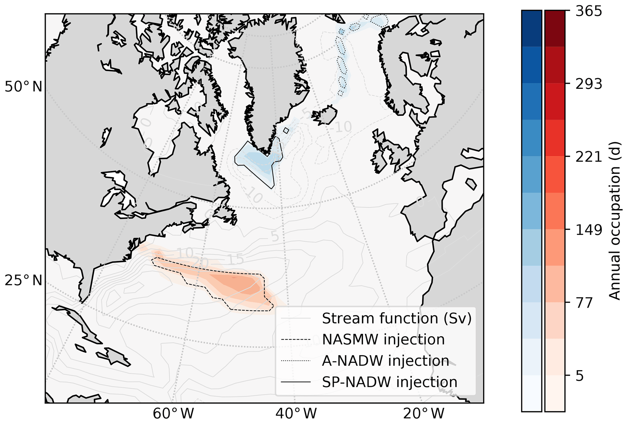
Figure 1Outcrop locations of NASMW (red) and NADW (blue) from a 60-year climatology of the nonlinear model, following their respective definitions in Sects. 3 and 4. Shading indicates the number of days of the year when the water mass is found at a given latitude and longitude. Light grey contours show the time-mean barotropic stream function for the North Atlantic. The dashed (solid or dotted) contour shows the distribution of the dye injection which initialises the tangent-linear run for NASMW (SP-NADW or A-NADW) at the annual maximum – see Sects. 3.2 (4.2.1 or 4.2.2)
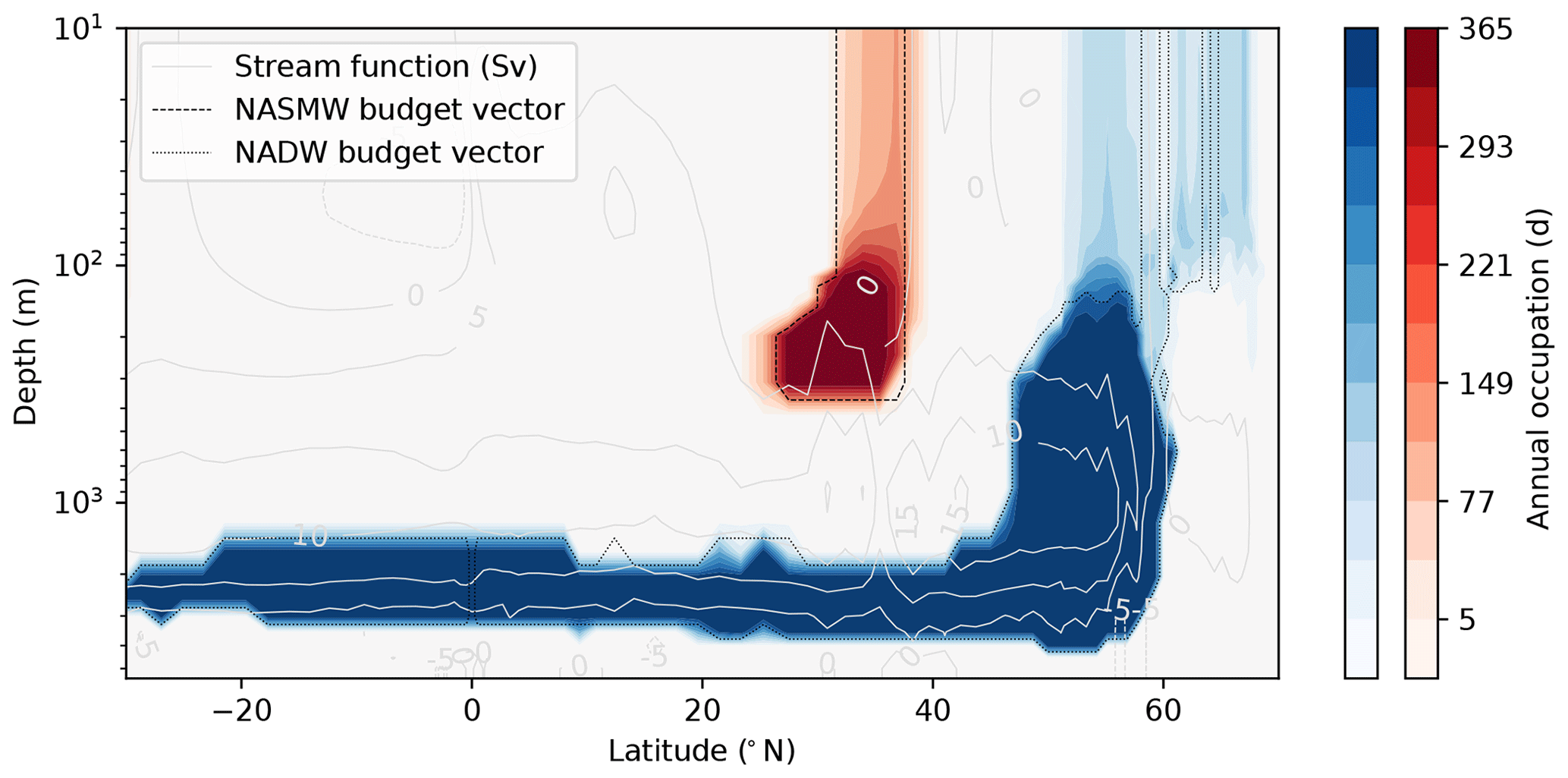
Figure 2Zonally averaged distribution of NASMW (red) and NADW (blue) in a 60-year climatology of the nonlinear model, following their respective definitions in Sects. 3 and 4. Shading indicates the number of days of the year when the water mass is found at a given latitude and depth. Light grey contours show the meridional stream function of the Atlantic. Dashed contours show the distribution at the point of the year when the adjoint run is started.
To isolate the purely passive response detailed in Eq. (4), we set velocity and sea surface height (SSH) modifications to zero in the NEMOTAM time stepping procedure (Fig. 3). Further feedbacks involving parameterisations such as vertical and eddy-induced mixing are already absent in NEMOTAM due to approximations in linearisation (Vidard et al., 2015) and so did not require further modification. Additionally, eddy-induced advective velocities are computed online by the nonlinear model and not stored explicitly in the trajectory. They may be recomputed from other trajectory variables, but this is not the default behaviour of NEMOTAM. As such, they were not included for the passive-tracer experiments in this study. They have been since been enabled in the passive-tracer source code as an optional online calculation. A preliminary comparative test suggests that errors are minor for our case studies (positive and negative concentration differences tend to cancel out, but even summing absolute differences, we do not exceed ∼ 6 % relative to the injection volume). We expect the difference to be greater in steep isopycnal regions such as the Southern Ocean.
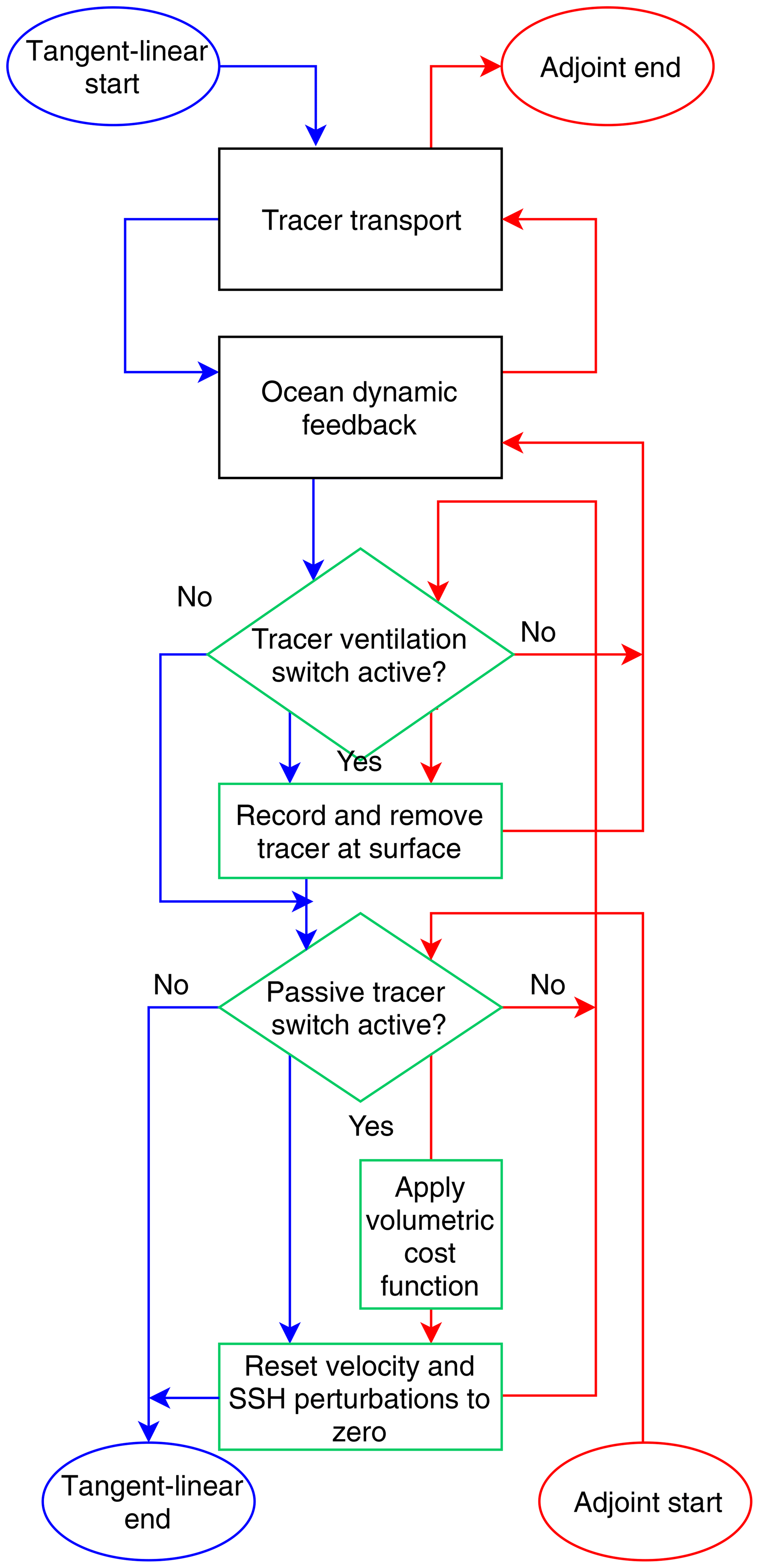
Figure 3Adaptation of NEMOTAM time-stepping procedure for the tangent-linear (blue) and adjoint (red) cases. Steps outlined in green are new additions to the scheme.
Our water mass tracking procedure is as follows. We begin by defining the water which we intend to track, for example using a temperature–salinity (TS) range. To track the evolution of newly formed water of this type, we identify all surface locations where T and S properties meet our definition in the nonlinear model trajectory. We then inject into the tangent-linear model a dye concentration of 1 in these locations and run the model forward. To identify the origins of existing water using the adjoint model, the procedure is similar. We begin by identifying model grid cells in the nonlinear trajectory (at all depths) which satisfy our TS definition. The budget vector is populated using the volume of these grid cells, with zero values elsewhere. This budget vector is then propagated back in time using the adjoint model to produce a sensitivity of the budget to earlier concentrations. In both cases, we remove any tracer which reaches the surface using the surface temperature-restoring scheme of the model. This scheme restores concentrations towards zero with a timescale of 60 days for a 50 m mixed layer (Madec, 2012). In the adjoint case, a record of this restoring leads to a spatio-temporal probability distribution of the surface origins of the tracer.
2.3 Advection schemes
The default advection scheme of the nonlinear model, used to compute the background state around which the model is linearised, is a total variation diminishing (TVD) scheme. This is a flux-corrected transport scheme (FCT; Lévy et al., 2001), which balances an upstream scheme with a centred scheme using a nonlinear weighting parameter described by Zalesak (1979). This scheme is preferable to others available in the model for non-eddying configurations (Lévy et al., 2001), but its nonlinearity means that it is not suitable for a TAM. As such, the standard advection scheme of NEMOTAM is a linearised counterpart in the form of a second-order forward-time–central-space (FTCS) finite difference scheme. A caveat of such schemes is the presence of an negative artificial diffusion coefficient, which can lead to negative quantities of positive-definite tracers (Owen, 1984). This encourages down-gradient diffusion of otherwise zero concentrations, acting as a source of further negative tracer when combined with the surface restoring scheme. This is particularly problematic in the case of passive-tracer advection as, unlike in the fully active TAM, negative quantities are unphysical.
An alternate scheme which is first-order linear (thus compatible with tangent-linear models and added to NEMOTAM for this study) is the trajectory-upstream scheme. This is an approximation to the classical upstream scheme, whereby the upstream direction is inferred from the trajectory velocity field (avoiding nonlinear sign functions). As the velocity field cannot be modified in the passive tracer case, however, the method is everywhere equivalent to the classical scheme. The scheme is forward in both time and space and offers the advantage of not producing negative tracer values. Nevertheless, this scheme also possesses an artificial (positive-valued) diffusion term, leading to a disproportionate spread of tracer, particularly in the vertical direction.
To strike a balance between the relative merits and caveats of the linear schemes described above, an approximation to the weighted-mean scheme of Fiadeiro and Veronis (1977) was coded into NEMOTAM. Like the TVD scheme, the true weighted-mean scheme is a linear combination of the classical upstream and FTCS methods. As before, we approximate the classical upstream method by using the trajectory-upstream scheme. The weighting parameter is determined dynamically from the trajectory. Strongly advective regions lean towards upstream advection, while strongly diffusive regions favour the centred formulation. Despite inheriting issues from both FTCS and the trajectory-upstream schemes, it is preferable to either of these individually. Its negative tracer concentrations are less persistent than those of the TVD and FTCS schemes, and its anomalous vertical spread was found to be less than half that of the upstream scheme (Fig. 4). Some issues have been raised with multivariate and time-dependent extrapolations of the weighted-mean scheme (e.g. Gresho and Lee, 1981). However, nonlinear flux-corrected transport schemes are required in order to improve on the weighted-mean scheme (Gerdes et al., 1991), and these are not compatible with the linear model. We thus proceed using our approximation to the weighted-mean scheme (in both the horizontal and vertical directions) for the water mass case studies detailed in this paper. We remark that it is entirely possible to incorporate a nonlinear advection scheme into NEMOTAM but that the resulting quasi-linear model would not have a true adjoint, which we require for our study.
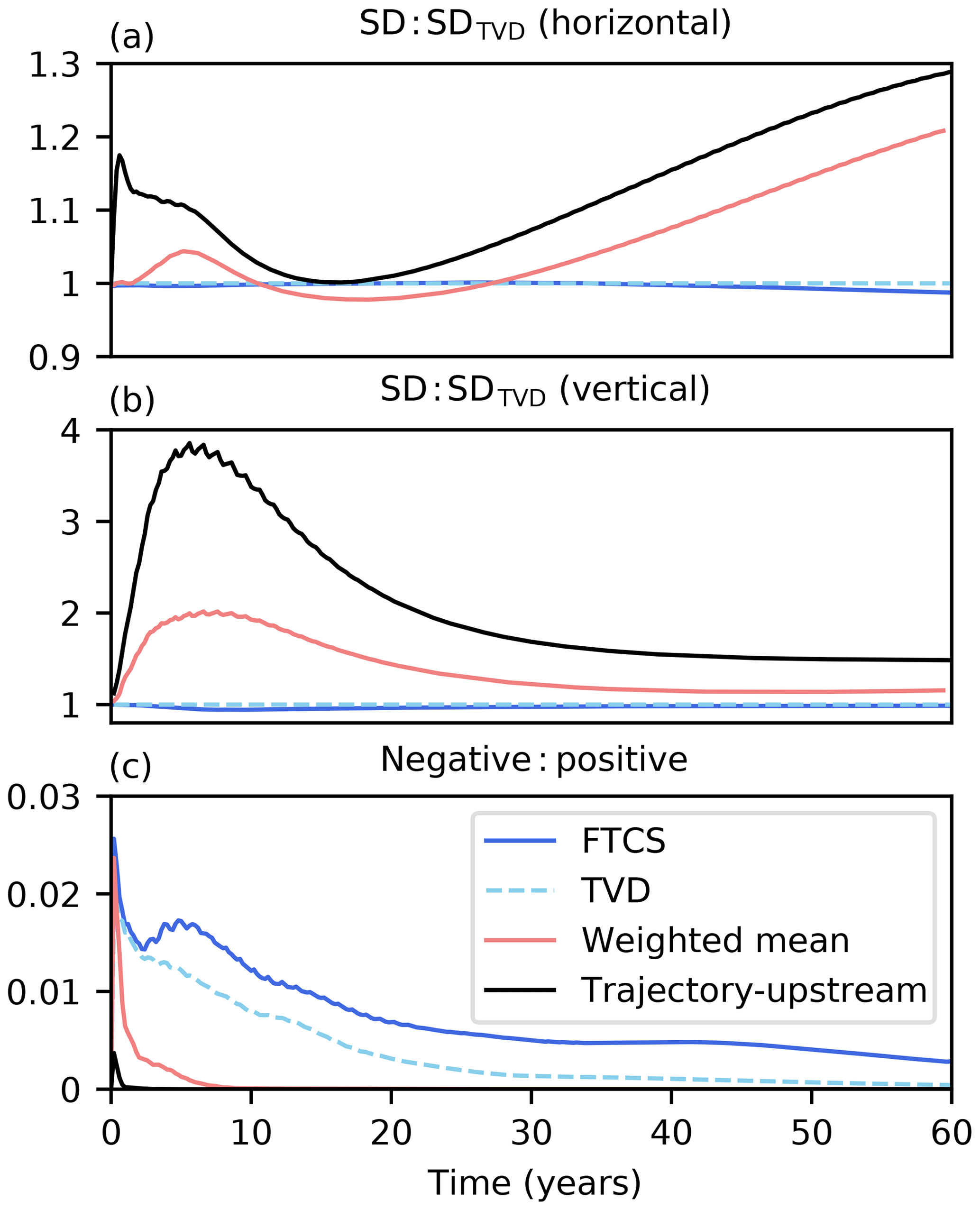
Figure 4Comparison of advection schemes in NEMOTAM. To assess the schemes, one of the runs of this study (the tangent-linear run of Sect. 3.2) was repeated with four different schemes, and the tracer distributions were compared. (a) Horizontal spread (spatial standard deviation around mean tracer position) as a ratio to the corresponding spread in the nonlinear TVD scheme. (b) Vertical spread (as above). (c) Ratio of volumes occupied by negative and positive tracer concentrations, respectively.
2.4 Performance
In order to test performance, the model was run for 100 d at 2∘ resolution (the ORCA2 configuration used in our case studies) and 5 d at 0.25∘ resolution (the ORCA025 configuration, Madec, 2012). Each configuration was run in four different modes (nonlinear, nonlinear with TAM trajectory production, tangent linear with passive tracer, and adjoint with passive tracer). Trajectory files were written once per day, and the linear advection scheme was the weighted-mean scheme described in Sect. 2.3. Each test was conducted with a range of parallelisation arrangements (16, 32, 64, 128, 256, and 512 CPU cores) and repeated 10 times to account for system variability (Table 1). The tests were conducted on a local HPC system, with 72 compute nodes, each offering two eight-core 2.6 GHz processors (Intel Xeon E5-2650 v2) and 64 GiB, connected by an InfiniBand QDR network.
Table 1Results of performance tests for two model configurations (ORCA2, upper section, and ORCA025, lower section). Top rows: trajectory storage requirements per output. Lower rows: runtime per model day for four model modes, including nonlinear with trajectory output (NLT), nonlinear without trajectory output (NL), tangent linear (TL), and adjoint (AD). The standard deviation of 10 runs is given as a ± uncertainty. Dashes indicate tests which failed due to insufficient memory.
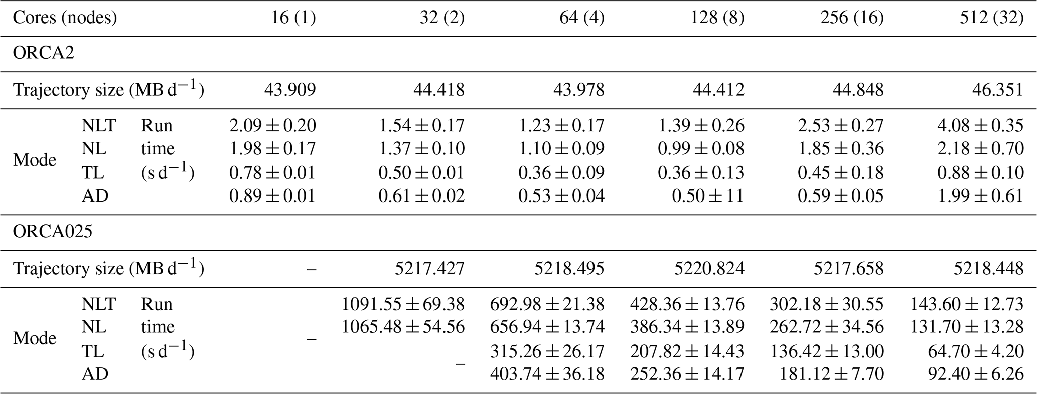
The general order of time efficiency is consistent across all tests; the linear forward model is between 2.5 (16 cores) and 3.1 (64 cores) times as fast as the nonlinear model without trajectory output in ORCA2 and from 1.9 (64 cores) to 2.0 (512 cores) times as fast in ORCA025. The adjoint is slightly less efficient. The nonlinear runs which produce trajectory output are the slowest across the board, due to the high level of output. Memory use appears higher in the linear model than the nonlinear, such that the linear model could not be run on two 64GiB compute nodes alone in ORCA025 (Table 1, column two).
The model shows good scaling in the ORCA025 configuration at all CPU arrangements tested here but begins to worsen in ORCA2 beyond 128 CPU cores. Further, the added time required for trajectory output in nonlinear ORCA2 runs on 128 CPU cores can be considerable. This is possibly due to the generation of a very large number of files during the model run, as the number of files generated is proportional to the number of CPU cores, the trajectory write frequency, and the run length. The required storage size remains relatively constant for runs with a larger number of CPU cores, despite the greater number of files (Table 1, row one).
An additional limitation which we discovered during our longest experiments comes from system file-number limits, which can readily be reached for typical systems for very long runs using many cores.
3.1 NASMW definition and properties
We now apply the developments of Sect. 2 to the problem of tracking the origins and fate of NASMW in the ORCA2-LIM simulation. There is no universally accepted definition of NASMW, with differing definitions leading to conflicting results between studies (Joyce, 2011). While the method allows us to define water masses in terms of any model variable, we choose for simplicity to utilise the common approach of a temperature–salinity range. In particular, we define model NASMW as water lying in the temperature band [17,19] ∘C, as in the original definition of Worthington (1959), with salinity in the range of [36.4,36.6] psu. As in some other studies (e.g. Kwon and Riser, 2004; Gary et al., 2014), we impose a third criterion, in our case that NASMW has a thickness of at least 125 m. This condition ensures homogeneity and isolates the water mass from the adjacent Madeira Mode Water (MMW) to its east (Siedler et al., 1987).
Model NASMW has a consistent outcrop in a single area (Fig. 1) and does not extend far south of its outcrop region below the surface (Fig. 2). The outcrop area of NASMW in the model peaks at the beginning of April at 1.3×10⁶ km2 (Fig. 5), coinciding with peaks in volume (4.2×10⁵ km3) and thickness (310 m) of the water mass. These maxima occur a month before the annual maximum local mixed layer depth (MLD) of 430 m. Following this, rapid stratification due to summer warming shoals the mixed layer. The outcrop area concurrently diminishes until the water mass is completely sheltered from air–sea exchange. This period of submergence extends from early June to early December, as the upper surface of the water mass progressively deepens to a maximum of 101 m. The volume also decreases, towards 1.3×10⁵ km3 at the annual minimum.
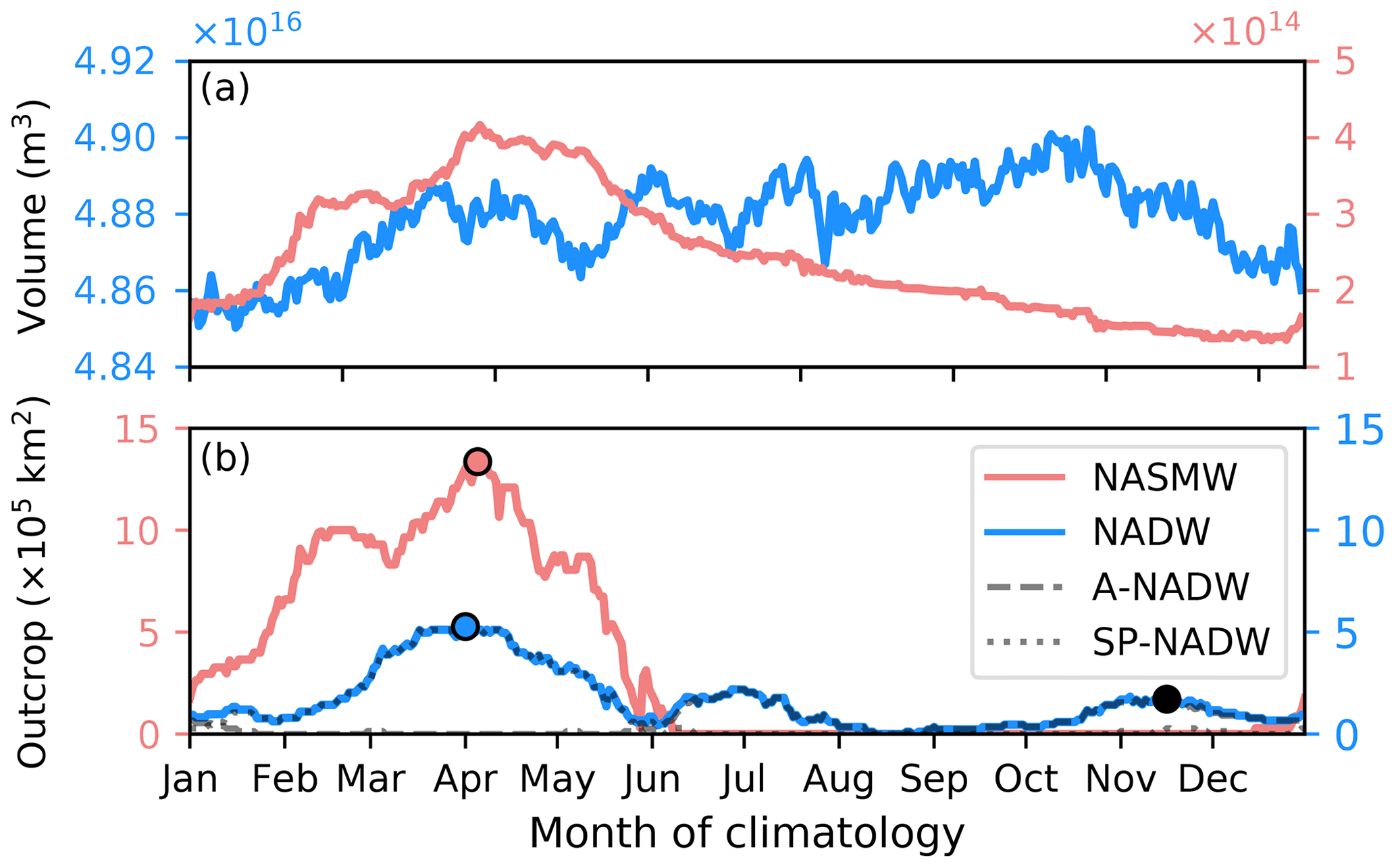
Figure 5Mean-year time series of NADW (blue) and NASMW (red) (a) volume and (b) outcrop surface area including those of the Arctic (dashed line) and subpolar (dotted line) NADW outcrops from the nonlinear trajectory. Circles indicate the injection time of NASMW (red), NADW (blue), and A-NADW (black) in the forward simulations (see Sects. 3.2 and 4.2).
3.2 Tangent-linear run
As outlined in Sect. 2.2, we begin by identifying all water matching our NASMW definition in the surface layer of the nonlinear model at a given time. We choose this to be the time when the outcrop is maximal (Fig. 5). We then inject a concentration of 1 into the tangent-linear model at these locations and propagate it for 60 years. Newly ventilated model NASMW initially resides close to the surface (Fig. 6). Here, its behaviour is governed by surface currents, which fractionate the water mass. At the point of application, 37 % of the tracer lies in the Gulf Stream. Most of this water follows the recirculation of the subtropical gyre, while a minority is exported to the subpolar region (2.5 % over 4 years). Our quantification of subpolar export is on the same order of that found under similar conditions by Burkholder and Lozier (2011), where inter-gyre exchange was studied in a purpose-built Lagrangian study.
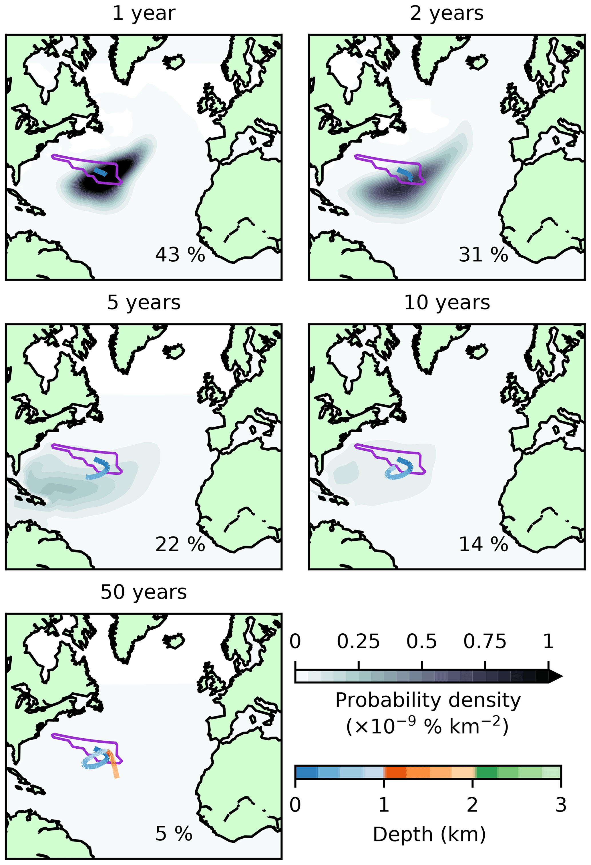
Figure 6Evolution of NASMW-tagged tracer in the tangent-linear model. Black and white shading indicates depth-integrated probability density (corresponding to the likelihood that NASMW is found in that region) at 1, 2, 5, 10, and 50 years. Inset percentages show the global integral of this field, i.e. the total proportion of tracer not yet re-ventilated at the surface. The coloured line tracks the centre of mass of the tracer from initialisation to its current position, with colours indicating the mean depth of the tracer. The purple contour shows the distribution of the original tracer injection.
Our NASMW is short lived. Persistent proximity to the surface leads to the re-ventilation of 95 % of the initialised tracer over the 60-year run. Of that which remains in the ocean, 90 % is transformed and no longer fits our definition of NASMW (Fig. 7). As time progresses, because of vertical mixing together with near-surface tracer removal by the restoring scheme, remaining tracer tends to reach deeper, colder, and fresher waters. Using the passive tracer approach, it is not possible to establish a full, qualitative description of the fate of NASMW. However, it can be observed that only around 5 % of all model NASMW re-ventilation occurs within its surface outcrop. The rest is mixed out of the TS class, either remaining in the system for the remainder of the 60-year simulation or (more commonly) resurfacing elsewhere.
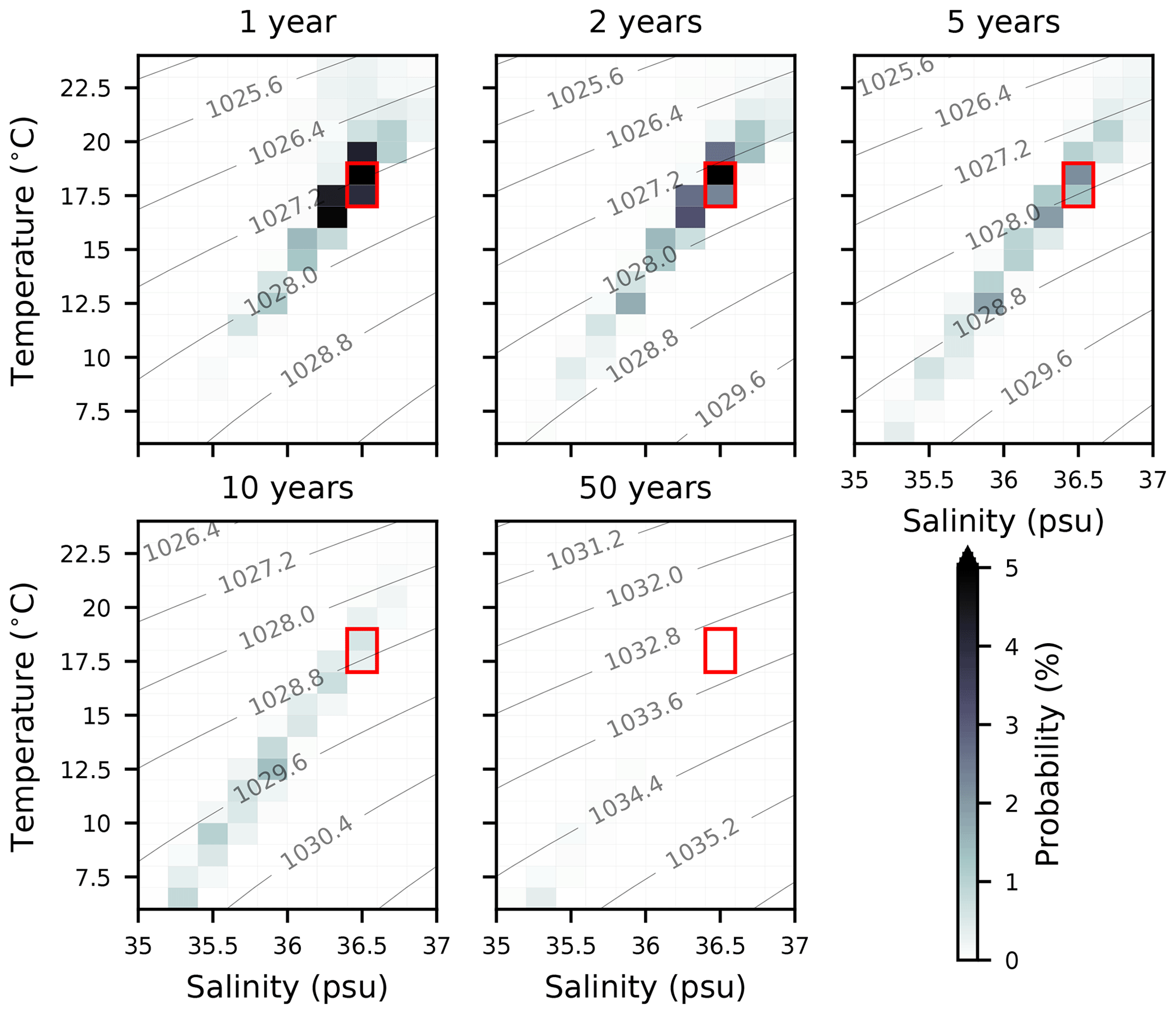
Figure 7Evolution of model NASMW in TS space. Shading indicates likelihood that the water mass found in a particular TS class after 1, 2, 5, 10, and 50 years. The red box marks the TS range used to define the water mass in this study. Contours show the density at the average depth level of the tracer.
Due to rapid re-exposure, the e-folding time of our NASMW is just 60 days. This is shorter than the estimations of Gary et al. (2014) (1 year) and Kwon et al. (2015) (3 years), but this is likely due to inherent differences in formulation. In the above studies, Lagrangian particles released in NASMW are not removed upon contact with the surface, so as to account for re-ventilation. Accounting for re-exposure, Fratantoni et al. (2013) suggest around 75 days, more closely aligned with our own findings.
3.3 Adjoint runs
To track existing model NASMW back to its source locations, we again follow the procedure outlined in Sect. 2.2. This consists of taking a budget of NASMW in the final year of a nonlinear simulation and propagating this budget backward using the adjoint model. We begin the adjoint run at the same point in the annual cycle as the tangent-linear run, when model NASMW volume is at its maximum (Fig. 5). We bisect the mode water budget co-vector 〈BMW| into tracer above the mixed layer depth () and tracer below ( and propagate each part separately. This allows us to explore the potential for a resilient layer of older NASMW below the MLD (Davis et al., 2013). By linearity, the union of the propagated budget vectors is equivalent to the propagated budget vector of NASMW as a whole, as follows:
Most NASMW propagated with the adjoint model reaches the surface quickly; 70 % of the tracer-tagged water mass is under 5 years old. During this early stage, ventilation occurs predominantly within the subtropical gyre recirculation, in the neighbourhood of the initial NASMW outcrop (Fig. 8). The 60-year mean formation location is also within this region, at 32∘ N, 58∘ W. This is almost coincident with the core of NASMW formation determined by Warren (1972) and agrees with the air–sea exchange-based estimate of Worthington (1959).
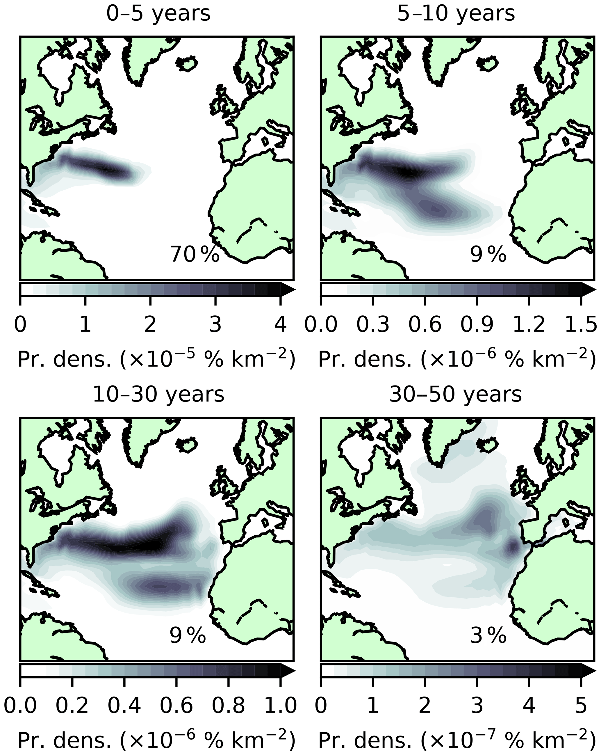
Figure 8Surface origins of model NASMW as determined by the backtracking budget analysis (adjoint model simulation). Shading indicates probability density. This corresponds to the likelihood that model NASMW is formed in a given region during the time periods [0,5], (5,10], (10,30], and (30,50] years. Inset percentages show the global integral (that is, the total proportion of the budget which is formed during each time period). Note that, contrary to Fig. 6, which displays instantaneous fields, here time-integrated fields are displayed. Due to the large variability in its extent over the integration window, the outcrop region is not shown.
For water over 5 years old, current patterns begin to have a distinct influence on formation. There is a clear signature of the Gulf Stream on the youngest model NASMW. This evolves backward as the adjoint propagates, eventually leaving an imprint of the entire subtropical gyre (Fig. 8). Simultaneously, newly formed mode water in the eastern North Atlantic (MMW) begins to cross into NASMW within 10 years. The signature of the Mediterranean outflow is particularly strong on the very oldest model NASMW, which also contains contributions from the subpolar region. The culmination of all of these water types throughout the 60-year evolution is evident when the sources of NASMW in the model are viewed in TS space (Fig. 9). Also apparent is that the primary source of NASMW has a warmer signature, which reflects the advection of warmer waters from the south, which cool and subduct to form the water mass. While the surface distribution suggests that a relatively small neighbourhood dominates the formation of model NASMW (Fig. 8), it should be borne in mind that the seasonal variability in surface properties (particularly the outcrop area) reflects strongly on the thermohaline properties of NASMW at formation (Fig. 9). This suggests that the NASMW surface outcrop is not, in fact, the dominant origin of NASMW in the model, contrary to the intuition provided by laminar models of the ventilated thermocline (e.g. Luyten et al., 1983). The implication is that mode water formation is not a passive process and that ocean dynamics must play a fundamental role.
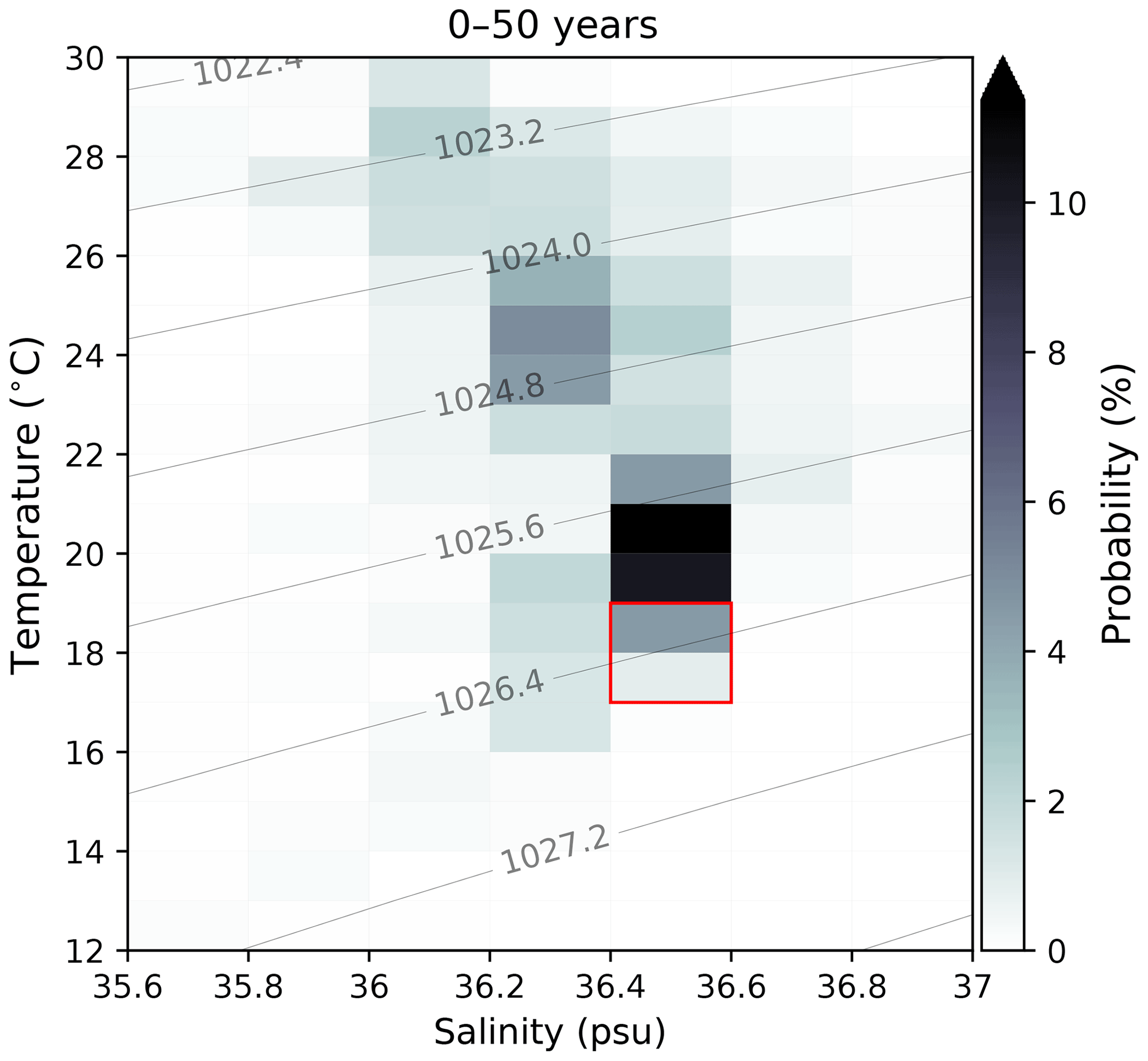
Figure 9Surface origins of model NASMW as determined by the backtracking budget analysis (adjoint model simulation) in TS space. Shading indicates the proportion of the budget originating from a particular TS class at the surface within 50 years. The red box marks the TS definition of NASMW used in this study. Contours show surface density.
We also consider the timescales involved with NASMW formation in the model. By recording the time at which tracer is removed from the budget by the surface restoring scheme, we may construct a probability distribution function (PDF) of water mass age (Fig. 10). There is a visibly lower skewness for NASMW lying below the MLD (Fig. 10, blue bars). Also clear is the seasonal cycle of shielding brought on by summer stratification, with less NASMW reaching the surface during these periods. Due to the simulation beginning at the annual maximum in NASMW production, peak NASMW formation occurs almost instantly. For tracer below the mixed layer (3.78 % of the total) the peak does not occur until the outcrop maximum of the third year. From the PDFs, the expected age of the model NASMW constituents above and below the MLD are, respectively, 4.70 and 8.79 years. It is evident that NASMW located below the MLD is shielded from renewal, with nearly double the expected age of model NASMW as a whole.
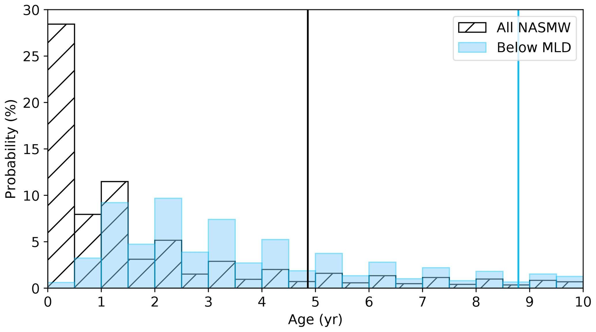
Figure 10Probability distribution of model NASMW age (hatched bars) and age of NASMW restricted to be found below the mixed layer depth (blue bars). The percentage of the NASMW budget formed in a given 0.5-year bin is indicated by its associated bar. The expected value of the distribution is marked by a solid line.
We finally address the asymptotic tail of the PDF, which represents the oldest waters found within NASMW. Our findings suggest a high-latitude source makes up a large fraction of this water, having followed a pathway from outside of our defined thermohaline range from the surface to eventually contribute to the makeup of NASMW (Fig. 8). Indeed, we find that for the period from 30 to 50 years, 68.3 % of NASMW originates at latitudes of 45∘ or higher. The idea of a distant source of the oldest NASMW is concurrent with the few studies which have considered it. Douglass et al. (2013) used an ideal-age tracer to construct a histogram similar to our own, acknowledging a remote source of the very oldest NASMW. Kwon et al. (2015) found that at least 20 % of NASMW stems from other regions and highlighted the potential importance of subpolar latitudes.
4.1 NADW definition and properties
As in Sect. 3.1, we now consider the properties and behaviour of NADW in the ORCA2-LIM simulation. We define NADW to fall within a temperature–salinity band of [2,4] ∘C and [34.9,35.0] psu, in close alignment with the definition of Worthington and Wright (1970). Analysis of the nonlinear model trajectory (about which the model is linearised) shows that there are two distinct latitudes at which water of this TS signature persistently outcrops in the simulation (Fig. 2, blue shading). These correspond to the (subpolar) Labrador–Irminger seas region, southwest of the Greenland–Scotland Ridge, and the (Arctic) Greenland Sea region, northeast of the ridge (Fig. 1, blue shading). The outcrop oscillates between the two regions with the seasonal cycle. While observed NADW is known to form only in extreme winters and has a strong interannual signature (Avsic et al., 2006), our use of repeated forcing implies that formation has little year-to-year variation. The Labrador–Irminger outcrop peaks at the end of March, around a month after the annual local mixed layer depth maximum of ∼ 1 km. At this peak, water in our NADW TS class occupies 5.3×10⁵ km2 at the surface (Fig. 5), before the area diminishes with the shoaling mixed layer. The Greenland Sea NADW outcrop in the model peaks in November, with a maximal extent of 2.3×10⁵ km2. At this time, surface NADW is exclusively found northeast of the Greenland–Scotland Ridge, and the water mass is shielded from ventilation elsewhere. On average, 66 % of the total annual outcrop area is southwest of the ridge, and 34 % is to its northeast.
Model NADW volume is almost constant year round at 4.9×10⁷ km3 (18.7 % of the model North Atlantic), deviating by less than 0.5 % annually.
4.2 Tangent-linear runs
As with NASMW, the dye injection |c0〉 coincides with the time step corresponding to the annual maximum outcrop extent, which here falls in April. It should be noted that all of the locations corresponding to this maximum are southwest of the Greenland–Scotland Ridge, in the subpolar Labrador–Irminger region. To investigate the nature of the Arctic outcrop, we follow a second injection of dye, in November, when its own outcrop extent is maximal. At this point, the water mass exclusively surfaces within the Arctic circle. We thus refer to these distinct surface waters as SP-NADW (for the southwestern, subpolar outcrop) and A-NADW (for the northeastern, Arctic outcrop). The tangent-linear model was run for 400 years with the SP-NADW dye injection and 60 years with the A-NADW dye injection. The run lengths were determined by the rate of surface tracer re-ventilation in each case.
4.2.1 SP-NADW
SP-NADW rapidly sinks, with tracer reaching an average depth of 1235 m after 0.2 years. It initially moves quickly westward, departing the surface region around Cape Farewell. It then spreads throughout the Labrador basin at depth and extends into the Irminger Sea (Fig. 11) at a temperature of 3.5 ∘C (Fig. 12). This initial behaviour is in broad agreement with temperature data from hydrographic sections (e.g. McCartney and Talley, 1982) and spatial distributions captured by chlorofluorocarbon (CFC) measurements (e.g. Rhein et al., 2002), floats (e.g. Bower et al., 2009) and models (e.g. Bower et al., 2011; Gary et al., 2011).
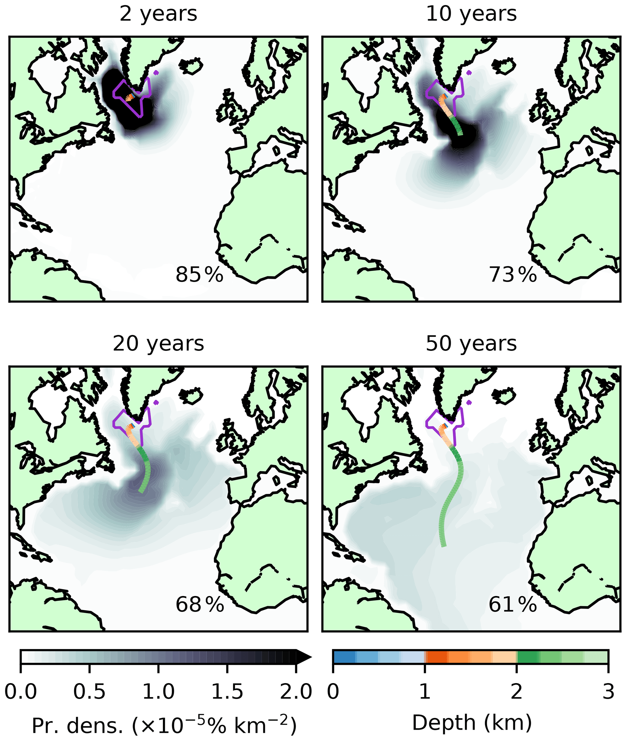
Figure 11As in Fig. 6 but for subpolar-outcropping model NADW and times of 2, 10, 20, and 50 years.
The tracer patch then moves southward, steadily deepening. Its deepest average point, 2466 m, is reached after some 22 years. Its mean position is at first closely tied to the DWBC. However, beyond the Flemish Cap, it takes a more central course through the basin interior. While interior southward routes generated by deep eddies have been found parallel to the DWBC in recent profiling float data (Lavender et al., 2000; Bower et al., 2009), our model configuration is non-eddying. As such, these pathways are represented by parameterised turbulent diffusion of the tracer, in a manner which would not be captured by Lagrangian drifters in our model (Gary et al., 2011).
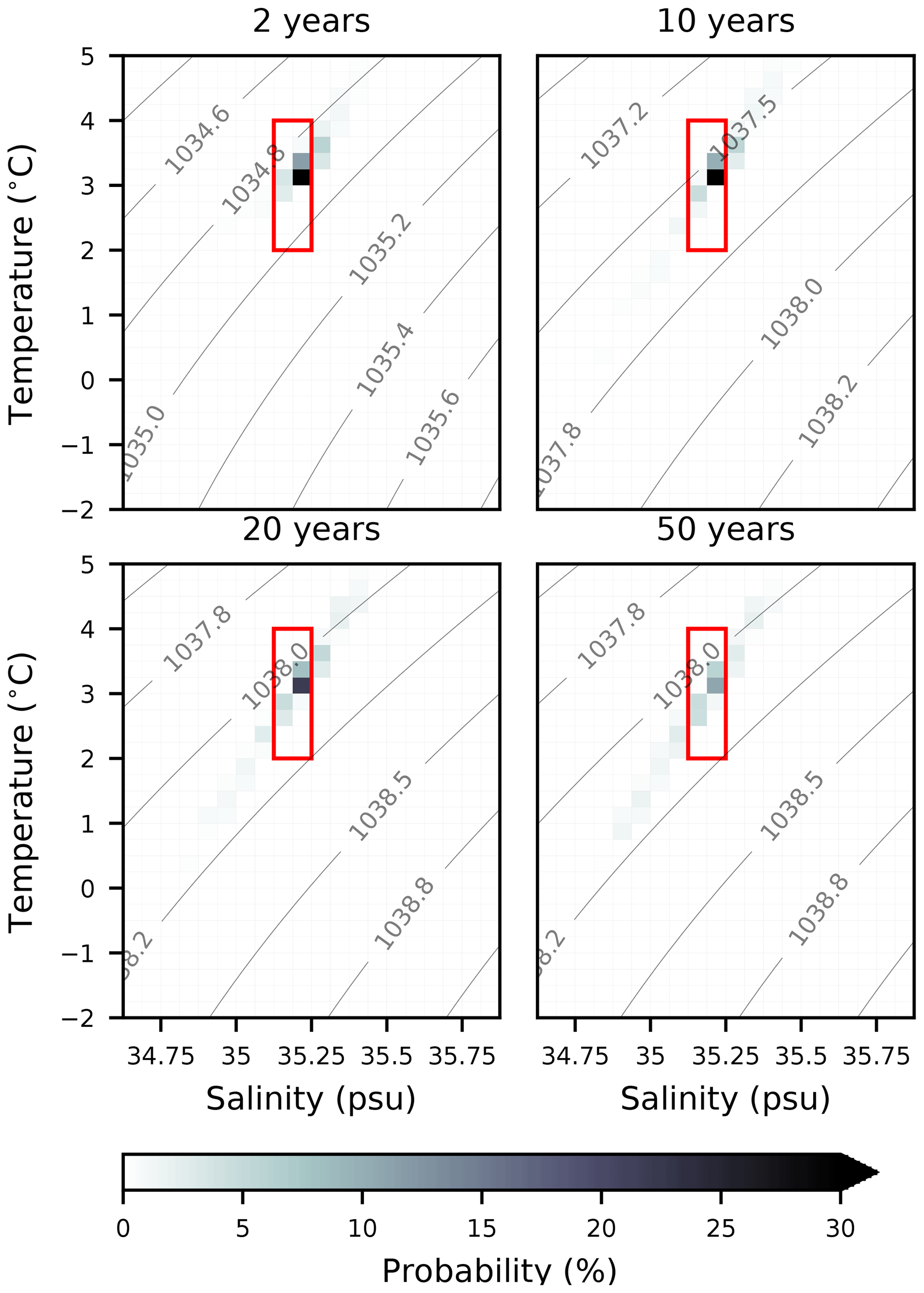
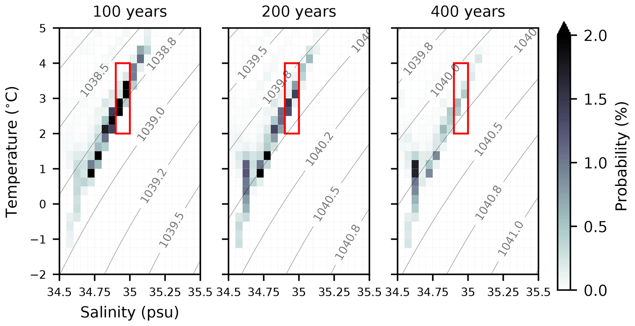
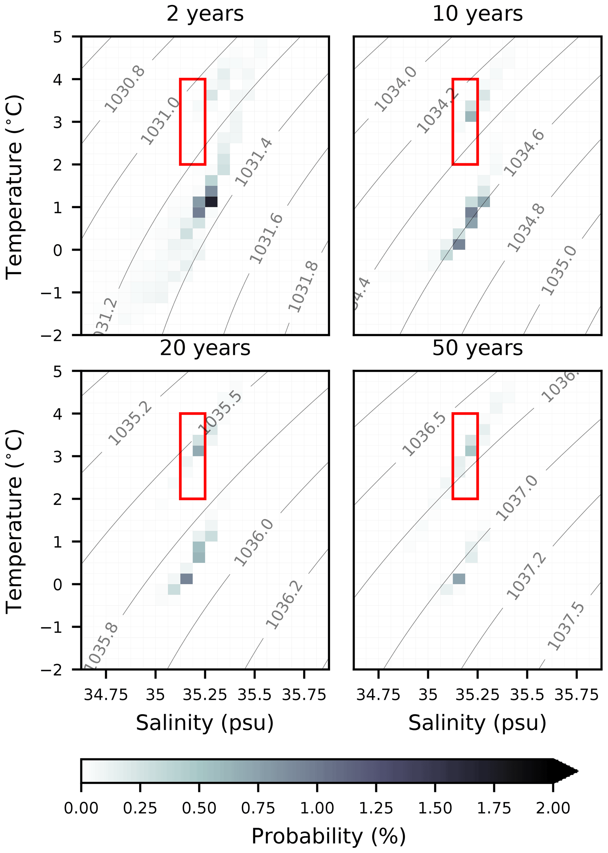
The tracer initialised in the model is quickly sequestered and is thus not vulnerable to re-exposure. Indeed, while 27 % of the initial volume of SP-NADW is re-ventilated within the first decade, only a further 24 % is removed during the rest of the century (Fig. 13). The homogeneity of the tracer is also preserved, with limited mixing into neighbouring TS classes on decadal timescales (48 % remains in the original TS class after 20 years, Fig. 12). There is a tendency over hundreds of years for the remaining water to cool and freshen to temperatures lower than 1.25 ∘C and salinities below 34.65 psu (Fig. 14). This follows the well-described behaviour of NADW following intrusion into the Southern Ocean. Observed NADW is known to mix into Circumpolar Deep Water, eventually transforming into bottom water with similar thermohaline characteristics to these (e.g. Orsi et al., 1999).
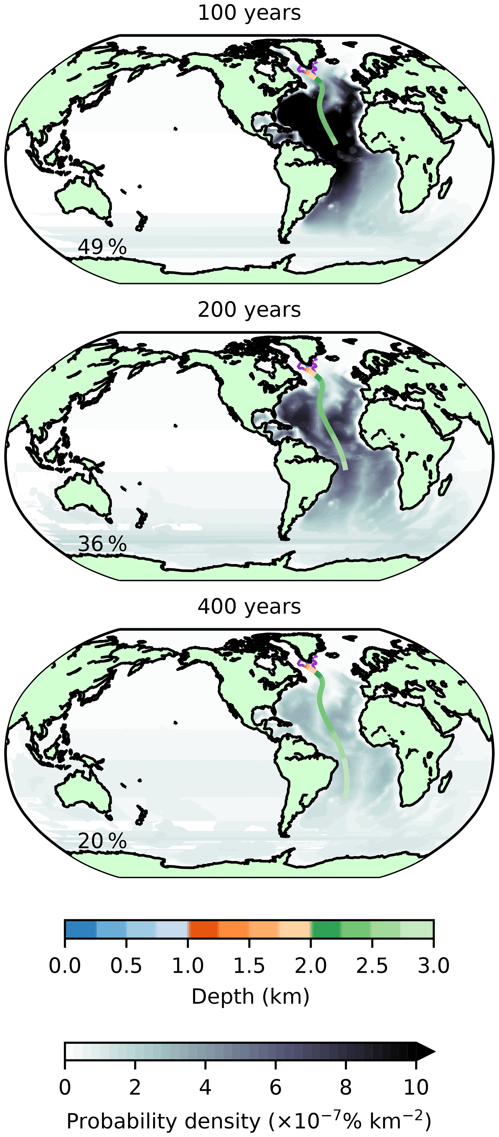
Figure 13As in Fig. 6 but for subpolar-outcropping model NADW and times of 100, 200, and 400 years.
4.2.2 A-NADW
The forward evolution of A-NADW (Fig. 15) is altogether different to SP-NADW, categorised by rapid diffusion and depletion. Unlike SP-NADW, which reaches great depths quickly following formation, A-NADW remains close to the surface on the Greenland and Barents shelves, with an average depth of only 502 m after 1 year. Due to this surface proximity throughout the run, the majority of tracer is re-exposed to the atmosphere. It is accordingly removed by the surface restoring scheme in the model, with 95 % of the initial volume removed after 20 years. That which remains either spreads throughout the Arctic ocean or spills over the shelf to join its SP-NADW counterpart in the Labrador Sea.
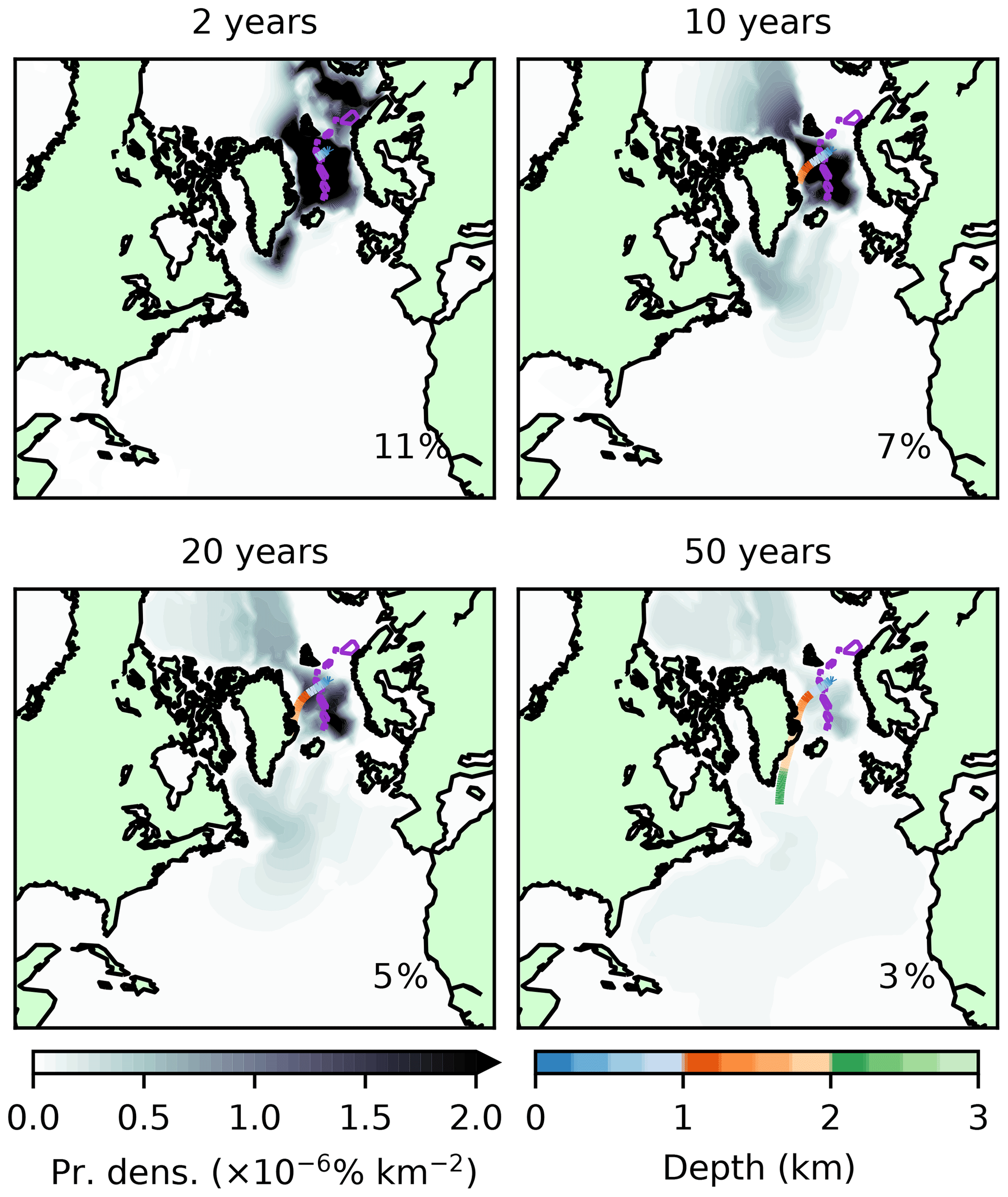
Figure 15As in Fig. 11 but for Arctic-outcropping model NADW.
Of all of the initialised A-NADW, that which ultimately reaches the Atlantic basin represents just 3.8 %. We may use the velocity fields of the nonlinear model to estimate transport pathways of this passive tracer into the basin. Consider an idealised case with two openings into the basin (here taken to represent the Denmark Strait and west of the Reykjanes Ridge), at points y1 and y2. The total volume flux into the basin between two times t0 and t1 will be approximately
where ci is the concentration of tracer at opening i, Δyi is the width of the opening, Δzi is the depth, ui is the velocity normal to ΔyiΔzi, t0 is the injection time, and t1 is 50 years later. As all of the above quantities are present in the model output, we may scale this approach up to the model grid and estimate each contribution. In this manner, we find that the vast majority of A-NADW destined for the North Atlantic (88 %) enters through the Denmark Strait.
Passive tracer injected at the A-NADW outcrop rapidly moves through TS space (Fig. 16). A colder, fresher water type splinters away from the surface-borne model NADW, and as a result, the tracer occupies two distinct regions in TS space for the remainder of the run. The warmer of these two water types shares most of its TS properties with those of the model NADW at the surface. On the other hand, the colder water type, at ∘C, bears a similar temperature signature to observed OW (LeBel et al., 2008).
Our simulation shows that surface-borne A-NADW does not proceed to form a substantial part of subsurface NADW in the simulation. Within 0.6 years, 78 % of the tracer has been re-exposed to the atmosphere. Of that which remains, some 98 % has left the NADW TS class. The little tracer which stays in our defined NADW class is persistent, eventually following a similar trajectory to SP-NADW through TS space.
The two tangent-linear experiments (following water from each of the two distinct NADW outcrop regions) suggest that the more northeasterly outcrop contributes quantitatively little to the NADW bulk. Hence, any surface origins of NADW in the Arctic of the model are likely found outside of the NADW TS class.
4.3 Adjoint run
As before, we take a water mass budget at the end of the nonlinear model simulation (in this case for NADW after 400 model years) and provide it to the adjoint model. Using this approach, 86 % of the NADW budget in model can be traced to its creation within 400 years (Fig. 17), with the rest remaining in the ocean interior.
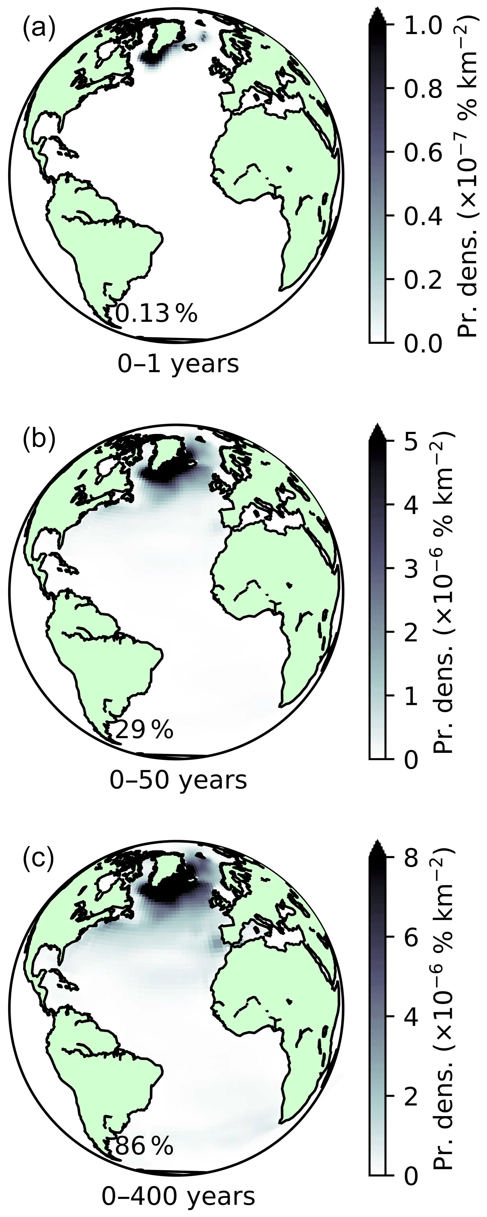
Figure 17As in Fig. 8 but for NADW and time periods (a) [0,1] years, (b) [0,50] years, and (c) [0,400] years.
During the first year, only 0.13 % of the total volume of model NADW is tracked back to the surface. The strong presence of shallower NADW during this period leads to a clean signature of the two outcrops (Fig. 17a). On multidecadal timescales, tracer from NADW can be traced back to locations spanning most of the northern North Atlantic (Fig. 17b), dominated still by the region surrounding its subpolar outcrop. Of particular interest on these timescales is the signature of the Mediterranean Outflow. It has been proposed from hydrographic data that the northward penetration of Mediterranean Water can intermittently reach the subpolar gyre, influencing LSW (Lozier and Stewart, 2008). However, we may only speculate as to whether this mechanism is present in our simulation.
Modelled NADW spanning the entire 400-year run (Fig. 17c) has sources throughout the Atlantic basin, with a notable contribution from the eastern boundary of the South Atlantic, local to the Benguela Current. The Labrador–Irminger sector remains the primary source of NADW at all considered timescales, however.
The propagated budget vector can be separated into different source regions and signatures. For instance, 31 % of the ventilated NADW can be traced back to the Irminger Sea, versus just 14 % to the Labrador Sea in the model. We may also construct a volumetric census of model NADW source waters in thermohaline space (Fig. 18a). This may further be partitioned into waters originating from the two climatic regions (i.e. subpolar and Arctic) associated with the distinct outcrops of NADW (Fig. 18b and c, respectively). Overall, 45 % of the total NADW formed during the 400-year run may be attributed to the subpolar region. The dominant TS class associated with NADW formation in the model matches that of our definition ([2,4] ∘C and [34.9,35.0] psu), though there are contributions from a cluster of subpolar water types in the range [2,10] ∘C and [34.5,35.5] psu. Despite the substantial seasonal surface exposure of NADW in the Arctic (34 % of the annual outcrop area; see Sect. 4.1), this region ultimately accounts for only 17 % of modelled NADW formation in 400 years. This agrees with our findings in the tangent-linear model (Sect. 4.2) that surface-borne NADW in the Arctic is subject to rapid re-ventilation and does not contribute to the NADW bulk. It further suggests that there is no other narrowly defined TS band which outcrops in the Arctic from which modelled Arctic NADW originates. As such, NADW from this region generally derives from a broad range of waters colder and fresher than we define NADW to be.
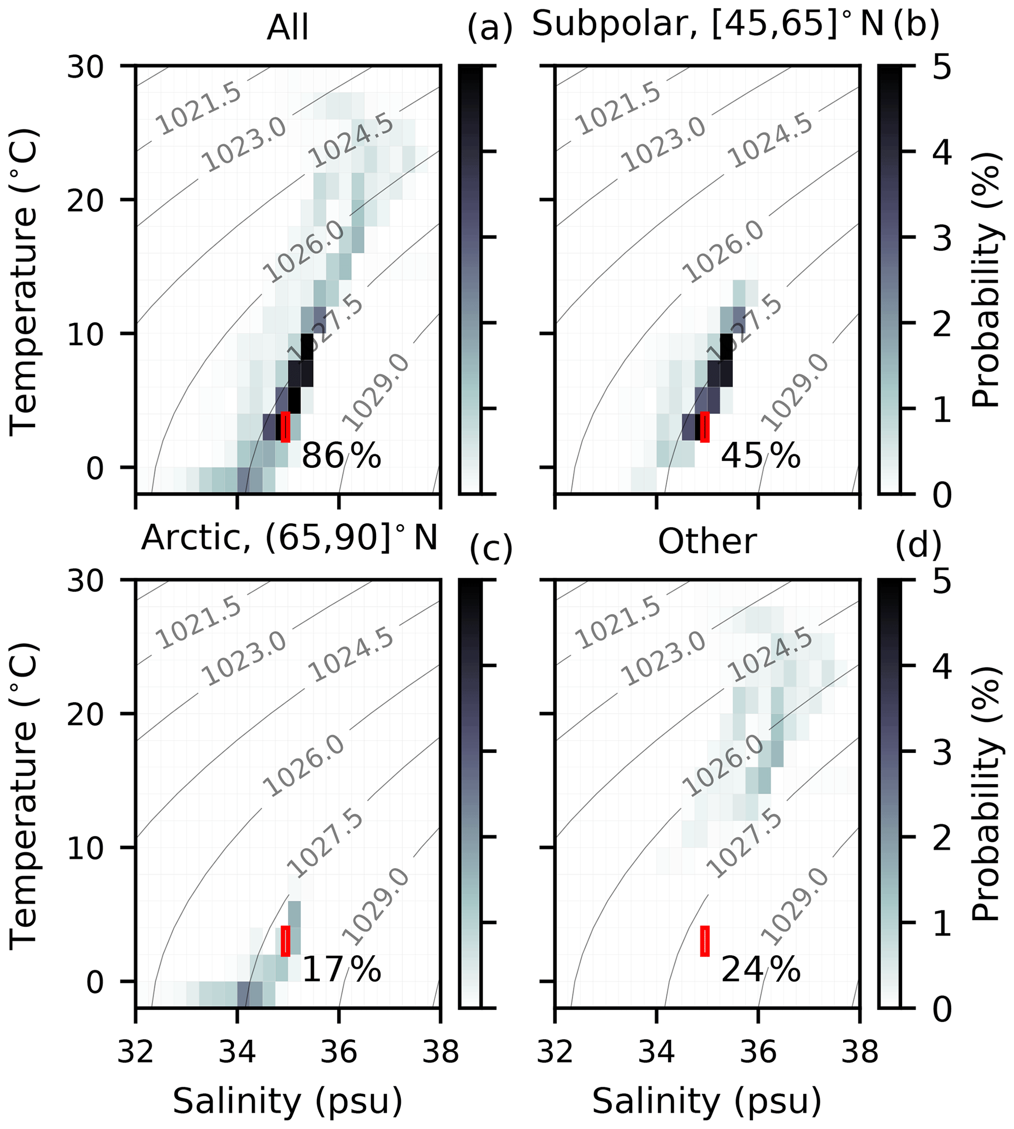
Figure 18As in Fig. 9 but for NADW and a time period of [0,400] years. (a) NADW total volume. (b) NADW volume traced to the subpolar North Atlantic. (c) NADW volume traced to the Arctic. (d) Volume of NADW originating elsewhere.
NADW that does not originate from either of these two regions of the North Atlantic makes up a substantial proportion (24 %; Fig. 18d) of the budget. Of this, 4 % is formed at high latitudes in the Southern hemisphere. Overall, 5 % of the total originates from outside the Atlantic.
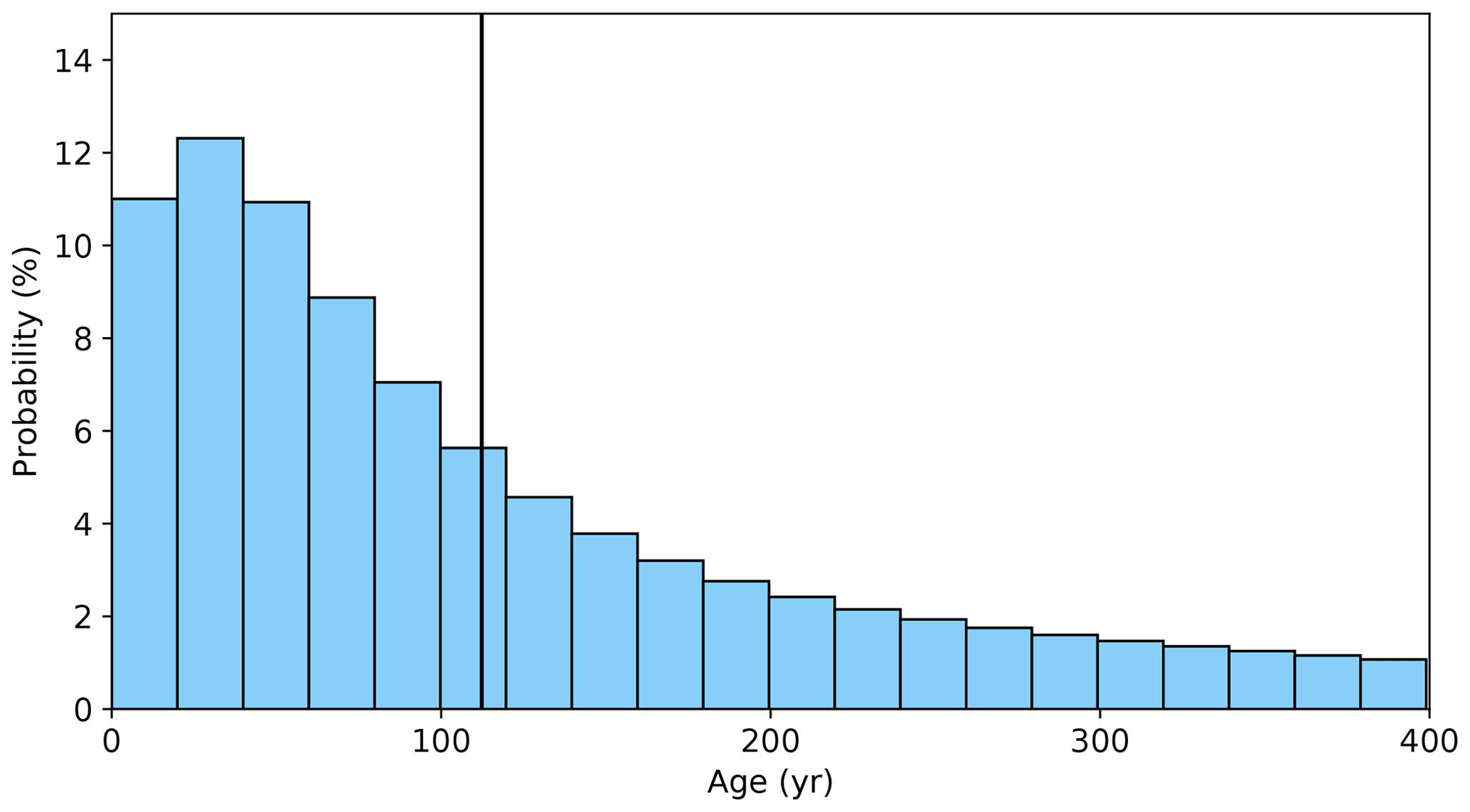
As in Sect. 3, we may also consider the temporal distribution of simulated NADW formation (Fig. 19). Age peaks in the 13th year, during which 0.6 % of the total budget can be traced back to the surface. The expected age is 112 years. It should be noted that the mean age of model NADW is likely slightly higher. As with any water mass studied in this manner, a proportion will always remain in the ocean (closing the overall budget). Due to this, surface ventilation does not quite account for 100 % of the total budget during our 400-year run. We limit our runs to this length due to technical constraints. In Sect. 3.3, we remarked on the unusual formation regions associated with the very oldest North Atlantic Subtropical Mode Water. This was associated with its much shorter life cycle. As such, the corresponding tail of the PDF of NADW age holds fewer surprises. Much like the youngest NADW considered here, the oldest NADW originates predominantly from winter convection in the Labrador and Irminger seas of the model.
We have presented a newly developed addition to the NEMOTAM tangent-linear and adjoint modelling framework for the NEMO OGCM. This package allows tangent-linear and adjoint tracking of passive-tracer transport. Our framework is rooted in concentrations and probabilities, comparable to the statistical properties of a high-resolution Lagrangian approach with a large (theoretically infinite) number of particles. The development was achieved by deactivating dynamic feedbacks in the time-stepping routine of NEMOTAM and embedding an alternative advection scheme suitable for passive-tracer transport. This advection scheme, proposed by Fiadeiro and Veronis (1977), is constructed as a linear combination of the upstream and centred schemes, so as to reduce spurious numerical diffusion. Performance tests show good scaling up to 128 cores at 2∘ resolution and up to at least 512 cores at 0.25∘ resolution, with much shorter run times (but higher memory demand) in the linear model with passive-tracer transport when compared with the fully active nonlinear model.
We have exhibited the use of this tool in two case studies concerning the tracking of North Atlantic-borne water masses, North Atlantic Subtropical Mode Water, and North Atlantic Deep Water. The versatility of the method has been demonstrated through the calculation of several quantities pertaining to these water masses. If a sufficiently long trajectory is used, a near-complete statistical distribution of surface formation can be constructed. This allows diagnosis of expected age and expected origin location, as well as the rate of eradication and re-ventilation of newly ventilated waters.
The linearity of the method ensures that the water being tracked can be partitioned into several components. When these components are propagated separately, the tracking of the whole is equivalent to the tracking of their union.
The results of our case studies show good agreement between the model configuration and common aspects of prior observational and computational studies. We have shown, for example, that, in our simulation, on average, the expected surface origin of tracer initialised within NASMW is 32∘ N, 58∘ W (in line with Worthington, 1959; Warren, 1972), that its decay time is around 2 months (as in Fratantoni et al., 2013), and that a small minority (2.5 % in 4 years) is exported to the subpolar gyre (concurrent with Burkholder and Lozier, 2011). We have estimated the average age of model NASMW as 4.5 years, also close to observations (e.g. Kwon and Riser, 2004), and shown that a more persistent NASMW subset (with an expected age of over 8.5 years) underlies the bulk of the water mass (as suggested by Davis et al., 2013).
For simulated NADW, we have shown (in the tangent-linear model) that an Arctic outcrop of water with its signature to the northeast of the Greenland–Scotland Ridge contributes little to its final form. However, we have found (by backtracking) that Arctic surface waters still make a contribution to simulated NADW formation (17 % here) but from a broad range in thermohaline space. It is understood that OW is produced by the cooling and freshening of North Atlantic inflow to the Greenland Sea (e.g. Quadfasel and Käse, 2007; Dickson et al., 2002). The finer details of this transformation and subsequent resupply of the transformed water into the North Atlantic are not well described by the method. The relative importance of pathways into the Atlantic for shelf water are still poorly known (Macrander et al., 2005), but we find using a broad transport estimate that the Denmark Strait is dominant in the model. For NADW formed in the subpolar outcrop of the Labrador Sea in the model, our tracer spread reflects well that observed using CFCs (e.g. Rhein et al., 2002). The diffusive behaviour of the passive tracer also means that, despite the non-eddying nature of our model, eddy-driven southward export pathways are better represented than they would be by Lagrangian drifters (e.g. Gary et al., 2011).
Nevertheless, there are several more intricate details of North Atlantic water mass formation and transport which are the subject of ongoing investigation and as such deserve a dedicated study at higher resolution. For example, the importance of fine-scale bathymetry for an accurate description of on-shelf NADW formation is well described (Hansen et al., 2001; LeBel et al., 2008; Smethie Jr. and Fine, 2001; Dickson et al., 2002). From a selection of models, Chang et al. (2009) found that the contribution of overflow waters to NADW is misrepresented by models coarser than in their study. In such models, the Faroe Bank Channel is typically unresolved, and the Denmark Strait Overflow resultantly dominates, as is the case here. Furthermore, although our tracer qualitatively reproduces southward export of LSW more effectively than a Lagrangian approach would in a laminar model, diffusion is still parameterised. It is unknown how well this parameterisation represents sub-grid-scale mixing for such processes.
Despite good broad agreement between the passive-tracer pathways and those noted in previous studies of these water masses, there is an interesting disparity between the forward and backward modes within the TAM itself. This originates from using a TS-based description to inform the initial tracer distribution. For example, the backtracking method suggests that NASMW predominantly originates in slightly warmer surface waters than those of the outcrop used to inform the forward model. Meanwhile, A-NADW, while occupying over a third of the simulated NADW annual outcrop, ultimately contributes almost nothing to the subsurface water mass. These deviations highlight the approximation used by many water-mass-tracking model studies – thermohaline characteristics are not a purely passive tracer. Water parcels experience changes in their thermohaline properties, and so water in a particular TS class at depth is not exclusively related to the same TS class at the surface through a passive advection pathway.
TAM use at high resolution is typically limited, due to baroclinic instability. However, this is not detrimental for passive tracer tracking, due to lack of dynamic feedbacks. As such, our tool may be used in conjunction with higher-resolution configurations of NEMO (e.g. ORCA12, Treguier et al., 2017). The main barrier to higher resolution for users of our development is the necessity of frequent output and storage of trajectory snapshots from the nonlinear model, which are required for NEMOTAM operation (Vidard et al., 2015). Future versions of our tool will allow regional trajectory storage to overcome this barrier.
Although we have presented the development in the context of water mass tracking, there are many potential further applications. Ocean heat uptake pathways and carbon sequestration have been studied by means of modelled passive tracers (e.g. Banks and Gregory, 2006; Xie and Vallis, 2012) and adjoint models (e.g. Hill et al., 2004). A slight modification to ignore vertical velocities read from the trajectory would force positive buoyancy on the tracer. This could allow buoyant anthropogenic pollutants to be tracked, with potential application to ocean plastic tracking and oil spill drift prediction. Water mass tracking may itself be complemented by considering continuous (rather than instantaneous) inputs of tracer at the surface. It is hoped that an off-the-shelf tool, bolted onto an existing OGCM will stimulate further research in these areas.
Despite TAM use for sensitivity analysis being traceable to the 1940s (Park and Xu, 2013), its application to ocean science is still in its infancy. The TAM approach is highly versatile, and its application to state-of-the-art OGCMs permits a great many new insights into ocean dynamics. Our development demonstrates the ability of a tangent-linear and adjoint model among the suite of existing water mass tracking methods. It is hoped that this novel tool will encourage new users to realise the potential of this powerful branch of ocean modelling.
NEMO v3.4 is available from https://forge.ipsl.jussieu.fr/nemo/svn/NEMO/releases/release-3.4 (last access: 16 April 2020) under the CeCILL licence. The configuration presented here is archived on Zenodo for general use (Stephenson, 2019a). The forcing files used in the simulations detailed here are also archived on Zenodo (NEMO Consortium, 2013), as are exact scripts and input files to reproduce our experiments and diagnostics (Stephenson, 2019b).
DS co-developed the source code, ran simulations, and wrote this paper. The development of the source code was overseen by SM, who provided further suggestions and additional technical assistance. FS proposed and supervised the project and assisted with experiment design. All authors discussed and contributed to the final paper.
The authors declare that they have no conflict of interest.
This research was supported by the Natural and Environmental Research Council UK (SMURPHS, grant no. NE/N005767/1, and MESO-CLIP, grant no. NE/K005928/1, and the SPITFIRE DTP) and the DECLIC and Meso-Var-Clim projects funded through the French CNRS–INSU LEFE programme.
This paper was edited by Qiang Wang and reviewed by Erik van Sebille and one anonymous referee.
Avsic, T., Karstensen, J., Send, U., and Fischer, J.: Interannual variability of newly formed Labrador Sea Water from 1994 to 2005, Geophys. Res. Lett., 33, L21S02, https://doi.org/10.1029/2006GL026913, 2006. a
Banks, H. T. and Gregory, J. M.: Mechanisms of ocean heat uptake in a coupled climate model and the implications for tracer based predictions of ocean heat uptake, Geophys. Res. Lett., 33, L07608, https://doi.org/10.1029/2005GL0253522006. a
Blanke, B. and Raynaud, S.: Kinematics of the Pacific equatorial undercurrent: An Eulerian and Lagrangian approach from GCM results, J. Phys. Oceanogr., 27, 1038–1053, 1997. a
Bower, A., Lozier, S., and Gary, S.: Export of Labrador Sea water from the subpolar North Atlantic: a Lagrangian perspective, Deep-Sea Res. Pt. II, 58, 1798–1818, 2011. a, b
Bower, A., Lozier, S., Biastoch, A., Drouin, K., Foukal, N., Furey, H., Lankhorst, M., Rühs, S., and Zou, S.: Lagrangian Views of the Pathways of the Atlantic Meridional Overturning Circulation, J. Geophys. Res.-Oceans, 124, 5313–5335, https://doi.org/10.1029/2019JC015014, 2019. a
Bower, A. S., Lozier, M. S., Gary, S. F., and Böning, C. W.: Interior pathways of the North Atlantic meridional overturning circulation, Nature, 459, 243–247, 2009. a, b, c
Broecker, W. S.: A revised estimate for the radiocarbon age of North Atlantic Deep Water, J. Geophys. Res.-Oceans, 84, 3218–3226, 1979. a
Burkholder, K. C. and Lozier, M. S.: Subtropical to subpolar pathways in the North Atlantic: Deductions from Lagrangian trajectories, J. Geophys. Res.-Oceans, 116, C07017, https://doi.org/10.1029/2010JC006697, 2011. a, b
Chang, Y. S., Garraffo, Z. D., Peters, H., and Özgökmen, T. M.: Pathways of Nordic Overflows from climate model scale and eddy resolving simulations, Ocean Model., 29, 66–84, 2009. a
Clarke, R. A. and Gascard, J.-C.: The formation of Labrador Sea water – Part I: Large-scale processes, J. Phys. Oceanogr., 13, 1764–1778, 1983. a
Davis, X. J., Straneo, F., Kwon, Y. O., Kelly, K. A., and Toole, J. M.: Evolution and formation of North Atlantic Eighteen Degree Water in the Sargasso Sea from moored data, Deep-Sea Res. Pt. II, 91, 11–24, https://doi.org/10.1016/j.dsr2.2013.02.024, 2013. a, b, c
Dickson, B., Yashayaev, I., Meincke, J., Turrell, B., Dye, S., and Holfort, J.: Rapid freshening of the deep North Atlantic Ocean over the past four decades, Nature, 416, 832–837, 2002. a, b
Dirac, P. A. M.: A new notation for quantum mechanics, in: Mathematical Proceedings of the Cambridge Philosophical Society, vol. 35, 416–418, Cambridge Univ. Press, 1939. a
Douglass, E. M., Kwon, Y.-O., and Jayne, S. R.: A comparison of North Pacific and North Atlantic subtropical mode waters in a climatologically-forced model, Deep-Sea Res. Pt. II, 91, 139–151, 2013. a
England, M. H. and Maier-Reimer, E.: Using chemical tracers to assess ocean models, Rev. Geophys., 39, 29–70, 2001. a
Errico, R. M.: What Is an Adjoint Model?, B. Am. Meteorol. Soc., 78, 2577–2591, https://doi.org/10.1175/1520-0477(1997)078<2577:WIAAM>2.0.CO;2, 1997. a, b
Fiadeiro, M. E. and Veronis, G.: On weighted-mean schemes for the finite-difference approximation to the advection-diffusion equation, Tellus, 29, 512–522, 1977. a, b
Fichefet, T. and Maqueda, M. A. M.: Sensitivity of a global sea ice model to the treatment of ice thermodynamics and dynamics, J. Geophys. Res., 102, 12609–12646, https://doi.org/10.1029/97JC00480, 1997. a
Fischer, J. and Schott, F. A.: Labrador Sea Water tracked by profiling floats—From the boundary current into the open North Atlantic, J. Phys. Oceanogr., 32, 573–584, 2002. a
Forget, G., Maze, G., Buckley, M., and Marshall, J.: Estimated Seasonal Cycle of North Atlantic Eighteen Degree Water Volume, J. Phys. Oceanogr., 41, 269–286, https://doi.org/10.1175/2010JPO4257.1, 2011. a
Fratantoni, D. M., Kwon, Y.-O., and Hodges, B. A.: Direct observation of subtropical mode water circulation in the western North Atlantic Ocean, Deep-Sea Res. Pt. II, 91, 35–56, https://doi.org/10.1016/j.dsr2.2013.02.027, 2013. a, b, c, d
Fukumori, I., Lee, T., Cheng, B., and Menemenlis, D.: The origin, pathway, and destination of Niño-3 water estimated by a simulated passive tracer and its adjoint, J. Phys. Oceanogr., 34, 582–604, 2004. a, b
Gao, S., Qu, T., and Fukumori, I.: Effects of mixing on the subduction of South Pacific waters identified by a simulated passive tracer and its adjoint, Dynam. Atmos. Ocean., 51, 45–54, 2011. a
Gao, S., Qu, T., and Hu, D.: Origin and pathway of the Luzon Undercurrent identified by a simulated adjoint tracer, J. Geophys. Res.-Oceans, 117, C05011, https://doi.org/10.1029/2011JC007748, 2012. a
Gary, S. F., Lozier, M. S., Böning, C. W., and Biastoch, A.: Deciphering the pathways for the deep limb of the Meridional Overturning Circulation, Deep-Sea Res. Pt. II, 58, 1781–1797, 2011. a, b, c, d
Gary, S. F., Lozier, M. S., Kwon, Y.-O., and Park, J. J.: The fate of North Atlantic subtropical mode water in the FLAME model, J. Phys. Oceanogr., 44, 1354–1371, 2014. a, b, c, d, e
Gerdes, R., Köberle, C., and Willebrand, J.: The influence of numerical advection schemes on the results of ocean general circulation models, Clim. Dynam., 5, 211–226, 1991. a
Giering, R. and Kaminski, T.: Recipes for adjoint code construction, ACM T. Math. Software., 24, 437–474, 1998. a
Gresho, P. M. and Lee, R. L.: Don't suppress the wiggles—they're telling you something!, Comput. Fluid., 9, 223–253, 1981. a
Hansen, B. and Østerhus, S.: North Atlantic–Nordic seas exchanges, Prog. Oceanogr., 45, 109–208, 2000. a
Hansen, B., Turrell, W. R., and Osterhus, S.: Decreasing overflow from the Nordic seas into the Atlantic Ocean through the Faroe Bank channel since 1950, Nature, 411, 927–930, 2001. a, b
Hill, C., Bugnion, V., Follows, M., and Marshall, J.: Evaluating carbon sequestration efficiency in an ocean circulation model by adjoint sensitivity analysis, J. Geophys. Res.-Oceans, 109, C11005, https://doi.org/10.1029/2002JC001598, 2004. a
Hirst, A. C.: Determination of water component age in ocean models: Application to the fate of North Atlantic Deep Water, Ocean Model., 1, 81–94, 1999. a
Iselin, C. O.: The influence of vertical and lateral turbulence on the characteristics of the waters at mid-depths, Eos T. Am. Geophys. Un., 20, 414–417, 1939. a
Johnson, G. C.: Quantifying Antarctic bottom water and North Atlantic deep water volumes, J. Geophys. Res.-Oceans, 113, C05027, https://doi.org/10.1029/2007JC004477, 2008. a
Jong, M. F. and Steur, L.: Strong winter cooling over the Irminger Sea in winter 2014–2015, exceptional deep convection, and the emergence of anomalously low SST, Geophys. Res. Lett., 43, 7106–7113, 2016. a
Joyce, T. M.: New perspectives on eighteen-degree water formation in the North Atlantic, J. Oceanogr., 68, 45–52, https://doi.org/10.1007/s10872-011-0029-0, 2011. a, b, c
Khatiwala, S., Visbeck, M., and Cane, M. A.: Accelerated simulation of passive tracers in ocean circulation models, Ocean Model., 9, 51–69, 2005. a
Klein, B. and Hogg, N.: On the variability of 18 degree water formation as observed from moored instruments at 55∘ W, Deep-Sea Res. Pt. I, 43, 1777–1806, 1996. a
Kwon, Y. O. and Riser, S. C.: North Atlantic subtropical mode water: A history of ocean-atmosphere interaction 1961-2000, Geophys. Res. Lett., 31, L19307, https://doi.org/10.1029/2004GL021116, 2004. a, b
Kwon, Y. O. and Riser, S. C.: General circulation of the western subtropical North Atlantic observed using profiling floats, J. Geophys. Res.-Oceans, 110, 1–22, https://doi.org/10.1029/2005JC002909, 2005. a
Kwon, Y.-O., Park, J.-J., Gary, S. F., and Lozier, M. S.: Year-to-year reoutcropping of eighteen degree water in an eddy-resolving ocean simulation, J. Phys. Oceanogr., 45, 1189–1204, 2015. a, b
Large, W. G. and Yeager, S. G.: Diurnal to decadal global forcing for ocean and sea-ice models: the data sets and flux climatologies, NCAR Technical Note, NCAR/TN-460+STR, 2004. a
Lavender, K. L., Davis, R. E., and Owens, W. B.: Mid-depth recirculation observed in the interior Labrador and Irminger seas by direct velocity measurements, Nature, 407, 66–69, 2000. a
Leaman, K. D. and Harris, J. E.: On the average absolute transport of the deep western boundary currents east of Abaco Island, the Bahamas, J. Phys. Oceanogr., 20, 467–475, 1990. a
LeBel, D. A., Smethie Jr., W. M., Rhein, M., Kieke, D., Fine, R. A., Bullister, J. L., Min, D. H., Roether, W., Weiss, R. F., Andrié, C., and Smythe-Wright, D.: The formation rate of North Atlantic Deep Water and Eighteen Degree Water calculated from CFC-11 inventories observed during WOCE, Deep-Sea Res. Pt. I, 55, 891–910, 2008. a, b
Lévy, M., Estublier, A., and Madec, G.: Choice of an advection scheme for biogeochemical models, Geophys. Res. Lett., 28, 3725–3728, 2001. a, b
Lozier, M. S. and Stewart, N. M.: On the temporally varying northward penetration of Mediterranean Overflow Water and eastward penetration of Labrador Sea Water, J. Phys. Oceanogr., 38, 2097–2103, 2008. a
Luyten, J. R., Pedlosky, J., and Stommel, H.: The Ventilated Thermocline, J. Phys. Oceanogr., 13, 292–309, https://doi.org/10.1175/1520-0485(1983)013<0292:TVT>2.0.CO;2, 1983. a, b
Macrander, A., Send, U., Valdimarsson, H., Jónsson, S., and Käse, R. H.: Interannual changes in the overflow from the Nordic Seas into the Atlantic Ocean through Denmark Strait, Geophys. Res. Lett., 32, L06606, https://doi.org/10.1029/2004GL021463, 2005. a
Madec, G.: the NEMO team: Nemo ocean engine–Version 3.4, Note du Pôle de modélisation, Institut Pierre-Simon Laplace (IPSL), France, 2012. a, b, c, d
Madec, G. and Imbard, M.: A global ocean mesh to overcome the North Pole singularity, Climate Dynamics, 12, 381–388, https://doi.org/10.1007/BF00211684, 1996. a
Marotzke, J., Giering, R., Zhang, K. Q., Stammer, D., Hill, C., and Lee, T.: Construction of the adjoint MIT ocean general circulation model and application to Atlantic heat transport sensitivity, J. Geophys. Res.-Oceans, 104, 29529–29547, 1999. a
Marshall, J., Ferrari, R., Forget, G., Maze, G., Andersson, A., Bates, N., Dewar, W., Doney, S., Fratantoni, D., Joyce, T., and Straneo, F.: The CLIMODE field campaign: Observing the cycle of convection and restratification over the Gulf Stream, B. Am. Meteorol. Soc., 90, 1337–1350, 2009. a
McCartney, M. S. and Talley, L. D.: The subpolar mode water of the North Atlantic Ocean, J. Phys. Oceanogr., 12, 1169–1188, 1982. a, b
Molinari, R. L., Fine, R. A., and Johns, E.: The deep western boundary current in the tropical North Atlantic Ocean, Deep-Sea Res. Pt. I, 39, 1967–1984, 1992. a
NEMO Consortium: NEMO Reference configurations inputs, https://doi.org/10.5281/zenodo.1471702, 2013. a
Orsi, A., Johnson, G., and Bullister, J.: Circulation, mixing, and production of Antarctic Bottom Water, Prog. Oceanogr., 43, 55–109, 1999. a
Owen, A.: Artificial diffusion in the numerical modelling of the advective transport of salinity, Appl. Math. Model., 8, 116–120, 1984. a
Park, S. K. and Xu, L.: Data assimilation for atmospheric, oceanic and hydrologic applications, vol. 2, Springer Science & Business Media, 2013. a
Pickart, R. S., Spall, M. A., Ribergaard, M. H., Moore, G., and Milliff, R. F.: Deep convection in the Irminger Sea forced by the Greenland tip jet, Nature, 424, 152–156, 2003a. a
Pickart, R. S., Straneo, F., and Moore, G.: Is Labrador Sea water formed in the Irminger basin?, Deep-Sea Res. Pt. I, 50, 23–52, 2003b. a
Qu, T., Gao, S., Fukumori, I., Fine, R. A., and Lindstrom, E. J.: Origin and pathway of equatorial 13∘C water in the Pacific identified by a simulated passive tracer and its adjoint, J. Phys. Oceanogr., 39, 1836–1853, 2009. a
Qu, T., Gao, S., and Fukumori, I.: Formation of salinity maximum water and its contribution to the overturning circulation in the North Atlantic as revealed by a global general circulation model, J. Geophys. Res.-Oceans, 118, 1982–1994, 2013. a
Quadfasel, D. and Käse, R. H.: Present-day manifestation of the Nordic Seas overflows, in: Natural Gas Hydrates-Occurence, Distribution and Detection, edited by: Paull, C. K. and Dillon, W. P., Amerikan Geophysical Union, vol. 173, 75–89, American Geophysical Union, 2007. a, b
Reid, J. L. and Lynn, R. J.: On the influence of the Norwegian-Greenland and Weddell seas upon the bottom waters of the Indian and Pacific oceans, Deep-Sea Res., 18, 1063–1088, 1971. a
Rhein, M., Fischer, J., Smethie, W., Smythe-Wright, D., Weiss, R., Mertens, C., Min, D.-H., Fleischmann, U., and Putzka, A.: Labrador Sea Water: Pathways, CFC inventory, and formation rates, J. Phys. Oceanogr., 32, 648–665, 2002. a, b
Schuert, E. A.: Turbulent diffusion in the intermediate waters of the North Pacific Ocean, J. Geophys. Res., 75, 673–682, 1970. a
Sévellec, F. and Fedorov, A. V.: Stability of the Atlantic meridional overturning circulation and stratification in a zonally averaged ocean model: Effects of freshwater flux, Southern Ocean winds, and diapycnal diffusion, Deep-Sea Res. Pt. II, 58, 1927–1943, 2011. a
Siedler, G., Kuhl, A., and Zenk, W.: The Madeira mode water, J. Phys. Oceanogr., 17, 1561–1570, 1987. a
Smethie Jr., W. M. and Fine, R. A.: Rates of North Atlantic Deep Water formation calculated from chlorofluorocarbon inventories, Deep-Sea Res. Pt. I, 48, 189–215, 2001. a
Speer, K. and Tziperman, E.: Rates of water mass formation in the North Atlantic Ocean, J. Phys. Oceanogr., 22, 93–104, 1992. a
Stephenson, D.: ds4g15/PT_TAM_ORCA2 v1.0.3, https://doi.org/10.5281/zenodo.3635919, 2019a. a
Stephenson, D.: ds4g15/passive_experiments v1.0.1, https://doi.org/10.5281/zenodo.3471041, 2019b. a
Straneo, F., Pickart, R. S., and Lavender, K.: Spreading of Labrador sea water: an advective-diffusive study based on Lagrangian data, Deep-Sea Res. Pt. I, 50, 701–719, 2003. a
Swift, J. H., Aagaard, K., and Malmberg, S.-A.: The contribution of the Denmark Strait overflow to the deep North Atlantic, Deep-Sea Res. Pt. I, 27, 29–42, 1980. a
Talley, L. and McCartney, M.: Distribution and circulation of Labrador Sea water, J. Phys. Oceanogr., 12, 1189–1205, 1982. a
Thomas, L. N.: Destruction of potential vorticity by winds, J. Phys. Oceanogr., 35, 2457–2466, 2005. a
Thomson, C. W.: The Voyage of the “Challenger”: The Atlantic; a Preliminary Account of the General Results of the Exploring Voyage of HMS “Challenger” During the Year 1873 and the Early Part of the Year 1876, vol. 1, Macmillan and Company, 1877. a
Treguier, A. M., Barnier, B., Albert, A., Deshayes, J., leSommer, J., Lique, C., Molines, J.-M., Penduff, T., and Talandier, C.: ORCA12, a global ocean-ice model at : successes, shortcomings and their impact on ocean forecasting, in: EGU General Assembly Conference Abstracts, vol. 19, p. 17950, 2017. a
Vidard, A., Bouttier, P.-A., and Vigilant, F.: NEMOTAM: tangent and adjoint models for the ocean modelling platform NEMO, Geosci. Model Dev., 8, 1245–1257, https://doi.org/10.5194/gmd-8-1245-2015, 2015. a, b, c, d
Warren, B. A.: Insensitivity of subtropical mode water characteristics to meteorological fluctuations, Deep-Sea Res., 19, 1–19, 1972. a, b
Welander, P.: An advective model of the ocean thermocline, Tellus A, 11, 309–318, 1959. a
Welander, P.: The thermocline problem, Philos. T. R. Soc. A, 270, 415–421, 1971. a
Worthington, L. and Wright, W. R.: North Atlantic Ocean atlas of potential temperature and salinity in the deep water including temperature, salinity and oxygen profiles from the Erika Dan Cruise of 1962, Tech. rep., Woods Hole Oceanographic Institution, 1970. a
Worthington, L. V.: The 18∘ water in the Sargasso Sea, Deep-Sea Res., 5, 297–305, 1959. a, b, c, d
Worthington, L. V.: Negative oceanic heat flux as a cause of water-mass formation, J. Phys. Oceanogr., 2, 205–211, 1972. a
Xie, P. and Vallis, G. K.: The passive and active nature of ocean heat uptake in idealized climate change experiments, Clim. Dynam., 38, 667–684, 2012. a
Zalesak, S. T.: Fully multidimensional flux-corrected transport algorithms for fluids, J. Comput. Phys., 31, 335–362, 1979. a