the Creative Commons Attribution 4.0 License.
the Creative Commons Attribution 4.0 License.
 | 10 Mar 2020
EXPLUME v1.0: a model for personal exposure to ambient O3 and PM2.5
Myrto Valari
Konstandinos Markakis
Emilie Powaga
Bernard Collignan
Olivier Perrussel
This paper presents the first version of the regional-scale personal exposure model EXPLUME (EXposure to atmospheric PolLUtion ModEling). The model uses simulated gridded data of outdoor O3 and PM2.5 concentrations and several population and building-related datasets to simulate (1) space–time activity event sequences, (2) the infiltration of atmospheric contaminants indoors, and (3) daily aggregated personal exposure. The model is applied over the greater Paris region at 2 km×2 km resolution for the entire year of 2017. Annual averaged population exposure is discussed. We show that population mobility within the region, disregarding pollutant concentrations indoors, has only a small effect on average daily exposure. By contrast, considering the infiltration of PM2.5 in buildings decreases annual average exposure by 11 % (population average). Moreover, accounting for PM2.5 exposure during transportation (in vehicle, while waiting on subway platforms, and while crossing on-road tunnels) increases average population exposure by 5 %. We show that the spatial distribution of PM2.5 and O3 exposure is similar to the concentration maps over the region, but the exposure scale is very different when accounting for indoor exposure. We model large intra-population variability in PM2.5 exposure as a function of the transportation mode, especially for the upper percentiles of the distribution. Overall, 20 % of the population using bicycles or motorcycles is exposed to annual average PM2.5 concentrations above the EU target value (25 µg m−3), compared to 0 % for people travelling by car. Finally, we develop a 2050 horizon projection of the building stock to study how changes in the buildings' characteristics to comply with the thermal regulations will affect personal exposure. We show that exposure to ozone will decrease by as much as 14 % as a result of this projection, whereas there is no significant impact on exposure to PM2.5.
- Article
(3337 KB) - Full-text XML
-
Supplement
(1245 KB) - BibTeX
- EndNote


Air pollution is the first environmental health risk with significant effects on morbidity and mortality (Lim et al., 2012; WHO, 2013). Despite significant improvement in European air quality over the past decades, in 2017, approximately 77 % of the urban population was still exposed to PM2.5 concentrations exceeding the WHO air quality guidelines for health (14 % for O3) (EEA, 2019). More than half of the mortality burden attributed to exposure to suspended particles of an aerodynamic diameter less than 2.5 µg m−3 (PM2.5) in France occurs in cities of more than 100 000 inhabitants (Pascal et al., 2016). Several epidemiological studies have shown the adverse health effects of exposure to PM2.5. For instance, in France, in 2004–2006, about 3000 deaths per year were attributed to levels of PM2.5 exceeding the WHO guideline value in nine French urban areas participating in the Aphekom project (Pascal et al., 2013). Previous studies have shown that ozone exposure correlates with both morbidity and mortality (Sun et al., 2018; Di et al., 2017).
In the majority of these studies, the exposure surrogate associated with morbidity or mortality metrics is a spatially aggregated pollutant concentration from measurements at different sites over the urban agglomeration (Anderson et al., 2004; Bell et al., 2005). The underlying hypothesis here is that exposure is homogenous over the population. For this assumption to be valid, these studies are limited to small geographical zones where population density and pollutant concentrations are also homogenous (Sarnat et al., 2007). Several shortcomings of this approach have been raised in previous studies. On one hand, pollutant concentrations are spatially heterogeneous, especially within cities where different emission sources coexist and the presence of buildings imposes barriers to the dispersion of pollutants. For example, a Health Effects Institute report states that the zones most impacted by traffic-related pollution are up to 300–500 m from highways and other major roads, and when calculated for large cities in North America, that affects 30 %–45 % of the population (HEI, 2010). Intra-urban variability in pollutant concentration is a principal source of exposure misclassification in environmental epidemiology models, leading to errors in the evaluation of the health risk (Blair et al., 2007; Edwards and Keil, 2017). Furthermore, large variability in population exposure arises from human activity, population mobility, transport usage, and building characteristics (Georgopoulos et al., 2005). Therefore, to study the health risk on specific population groups – such as children, elderly people, asthma patients, or pregnant women (Olsson et al., 2014), or the health effects of co-pollutants (Olstrup et al., 2019b, a; Valari et al., 2011), or the risk associated with living or working near busy roads (Lipfert and Wyzga, 2008; Miranda et al., 2013) – one has to account for pollutant concentration at district level, population dynamics, and exposure indoors and during transport (Franklin et al., 2012; Hodas et al., 2012).
To answer this emerging demand, several methods for estimating personal exposure have been developed. Land-use regression models have been largely used to relate concentrations measured at monitor sites with concentration estimates at different locations across the city (Beelen et al., 2013; Cattani et al., 2017; Ryan and LeMasters, 2007). Then, space–time activity data are coupled to concentration data to provide exposure estimates (Vizcaino and Lavalle, 2018; Xu et al., 2019a). Land-use regression models provide spatial maps where urban features such as roads, buildings, and parks may be distinguished from background concentration levels. But concentration gradients resulting from the regression do not account for the dynamical or chemical processes taking place at these scales. Portable instruments, based on mass filters or high-accuracy optical methods (reference sensors), have also been used during specific field campaigns to measure exposure in cars, in subway trains, and on subway platforms, and in residences or other indoor microenvironmental locations (Hwang and Lee, 2018; Lim et al., 2012; Morales Betancourt et al., 2019; Williams and Knibbs, 2016; Xu et al., 2019b). These methods are accurate but restricted to limited periods and spatial contexts. The availability of low-cost personal monitors (microsensors) is a new opportunity in the atmospheric exposure field. They provide access to almost real-time, high-resolution concentration measurements (Xie et al., 2017). However, the accuracy of these instruments, their calibration, as well as their high sensitivity to environmental conditions (e.g. humidity) and human manipulation are yet to be addressed before their true potential is to be realized (Berchet et al., 2017).
Pollutant concentration fields simulated with atmospheric dispersion models are another possible input source for exposure models. The advantage of this approach is that simulation data may cover long time periods to support climate studies or policy applications adjusting for meteorological variability, emissions regulations, and land-use classification. Gaussian dispersion models have often been coupled with population space–time activity data for use in exposure studies (Dias and Tchepel, 2018; Korek et al., 2015; Batterman et al., 2014; Willers et al., 2013). These models, coupled with regional-scale chemistry–transport models, account simultaneously for long-range transport, regional background concentrations, and local features such as traffic emissions over the road network (Soares et al., 2014).
Regional-scale chemistry–transport models (CTMs) such as CHIMERE (Mailler et al., 2017) or the Community Multi-scale Air Quality model (CMAQ; Appel et al., 2014) have achieved resolution of 1 km×1 km with sufficient accuracy to be considered for use in such fine-scale applications (Beevers et al., 2013). Statistical, dynamical, or hybrid downscaling techniques such as kriging (Beauchamp et al., 2015) or subgrid-scale parameterizations (Valari and Menut, 2010) can be applied or coupled to these models to provide concentrations at district level. The use of CTMs instead of high-resolution Gaussian or Lagrangian models in an exposure context has several advantages. The study domain may be large enough to cover an entire region, whereas typical Gaussian or Lagrangian applications cover, at best, the urban agglomeration. However, a large part of the population moves in and out of the agglomeration within the day and on a systematic basis. Furthermore, the enhanced chemical mechanisms of CTMs compared to the simplified chemistry (the Chapman cycle) in Gaussian or Lagrangian models gives access to refined information on the chemical speciation and size distribution of particulate matter (PM). This information is particularly relevant in the context of health impact assessment, since the health impact of PM strongly depends on these properties (Atkinson et al., 2015; Cassee et al., 2013).
This paper presents the first version of a regional-scale model for personal exposure to O3 and PM2.5. The originality of the model lies in the development of (i) individual activity sequences that are defined geographically in space and time and (ii) the modelling of seasonal distributions of indoor ∕ outdoor ratios by building type and age. This latter feature is unique in personal exposure modelling since, typically, indoor pollutant concentrations rely on measurements for a few locations that may not represent the area's buildings. The model is developed as a post-processing tool for the CHIMERE regional-scale CTM and aims to facilitate health impact assessment. Outdoor pollutant concentrations are simulated with CHIMERE at 2 km×2 km resolution. The model selects sample populations that reproduce essential demographics at relevant geographical units (communes), namely age, gender, occupation, communes of residence and work, principal modes of transportation, and construction dates of residence and workplace. Activity event sequences for each member of the sample are developed by matching the distributions in the simulated population with distributions in the Enquête Globale de Transport (EGT, 2010) study. Infiltration of outdoor air pollution indoors in dwellings, offices, and schools is modelled with the Simulation of air RENewal (SIREN) model (Collignan et al., 2012), developed at the Centre Scientifique et Technique du Bâtiment (CSTB). SIREN is used to develop seasonal distributions of indoor ∕ outdoor ratios for each type of building. For other indoor locations (cars, buses, subway, and regional trains and trams), we apply indoor ∕ outdoor ratios found in the literature from previous measurement campaigns conducted in the region. Adjustments are also applied for specific activities such as cycling, walking on busy roads, and waiting on the subway platforms, as well as for car journeys that intersect tunnels or the Boulevard Periphèrique (ring road). Space–time activity sequences define the geographical coordinates of each member of the population at each minute of the simulation. Daily averaged personal exposure is calculated from the products of time spent by a person in different microenvironments and the time-averaged pollutant concentrations occurring in those locations (Klepeis, 2006). Personal exposure is simulated for the entire year of 2017 over the Île-de-France region (greater Paris).
The most accurate exposure assessment would rely on real-time personal monitoring devices affixed to people as they move within all the locations that are part of their daily routines (Klepeis, 2006). In practice, such equipment is too expensive to affix to large cohorts. Also questions such as the calibration of the monitors and the assessment of the uncertainties still need to be tackled before such studies could be carried out at regional scale. In a modelling framework, discrete locations (termed “microenvironments”) are considered rather than fully continuous space. In this case, the exposure trajectory of the receptor is followed explicitly. This approach has been adapted in cohort studies such as McBride et al. (2007). As in Klepeis (2006), in the exposure model developed here, receptors are simulated through individuals. Further discretizing in time, we calculate exposure as the sum of the product of time spent by a person in different microenvironments and the time-averaged pollutant concentrations occurring in those locations:
Here, Tij is the time spent in microenvironment j by person i with units in minutes, Cij is the air-pollutant concentration person i experiences in microenvironment j in units of µg m−3, Ei is the integrated exposure for person i (µg m−3 min), and m the number of different microenvironments. In this formulation, concentration Cij is averaged over the corresponding time period Tij .
The general structure of the model with the necessary input datasets for the exposure calculation is illustrated in Fig. 1. Outdoor pollutant concentrations are simulated with a regional-scale chemistry–transport model. We use hourly averaged data over a horizontal grid with 2 km spacing in both the west–east and the south–north directions (Sect. 3.1). Indoors pollutant concentrations (in buildings and during transportation) are deduced from outdoor concentrations by applying indoor ∕ outdoor ratios. The model does not account for indoor sources so far. For buildings, indoor ∕ outdoor ratios are calculated through a ventilation model (Sect. 3.2.1). For other indoor microenvironments, indoor ∕ outdoor ratios are either taken from previous studies in the Île-de-France region or calculated from existing indoor and outdoor concentration data, as is the case for subway platforms (Sect. 3.2.2).

Figure 1Overview of the EXposure to atmospheric PolLUtion ModEling (EXPLUME) model structure from the input data to the exposure calculation.
To obtain activity event sequences that determine the location of each member of the simulated population in time, we draw on the 2010 survey “Enquête globale de transport” (EGT, 2010) conducted by the Direction Régional et Interdépartemental de l'Equipement et de l'Aménagement d'Île-de-France. This survey questioned 43 000 individuals and identified 143 000 journeys. Each journey is characterized by the origin and destination points, the motive for travelling, the duration, and the means of transportation used. The mobility of the sample population is simulated with a Monte Carlo model that matches the simulated data with the EGT (2010) data (Sect. 4).
3.1 Outdoor O3 and PM2.5 concentration predictions
Pollutant concentrations are modelled with the CHIMERE model (Mailler et al., 2017) at a horizontal resolution of 2 km×2 km. Four-level one-way nesting is used for the CHIMERE simulation with grids of 60, 20, 7, and 2 km spacing between cells at both west–east and south–north directions. Overall, 15 vertical layers are used from 998 up to 300 hPa, with layers becoming thicker with distance from the surface level. Meteorological conditions are modelled with the Weather Research and Forecasting model (WRF; Skamarock et al., 2008) offline at the same four-level nesting grids as for the CHIMERE simulation but with a two-way nesting configuration. Global HTAP (Hemispheric Transport of Atmospheric Pollutants) anthropogenic emissions are used outside the European continent, European Monitoring and Evaluation Programme (EMEP) emissions for Europe outside the Île-de-France region, and finally a 1 km×1 km resolution bottom-up emission inventory developed by the AIRPARIF agency for anthropogenic emissions over the Île-de-France region.
Table 1Common metrics of statistical performance of the CHIMERE model, namely Pearson correlation, mean bias, and root mean square error, aggregated over the whole year of 2017, and for summer and winter seasons. Comparisons with traffic background and rural stations are conducted separately.
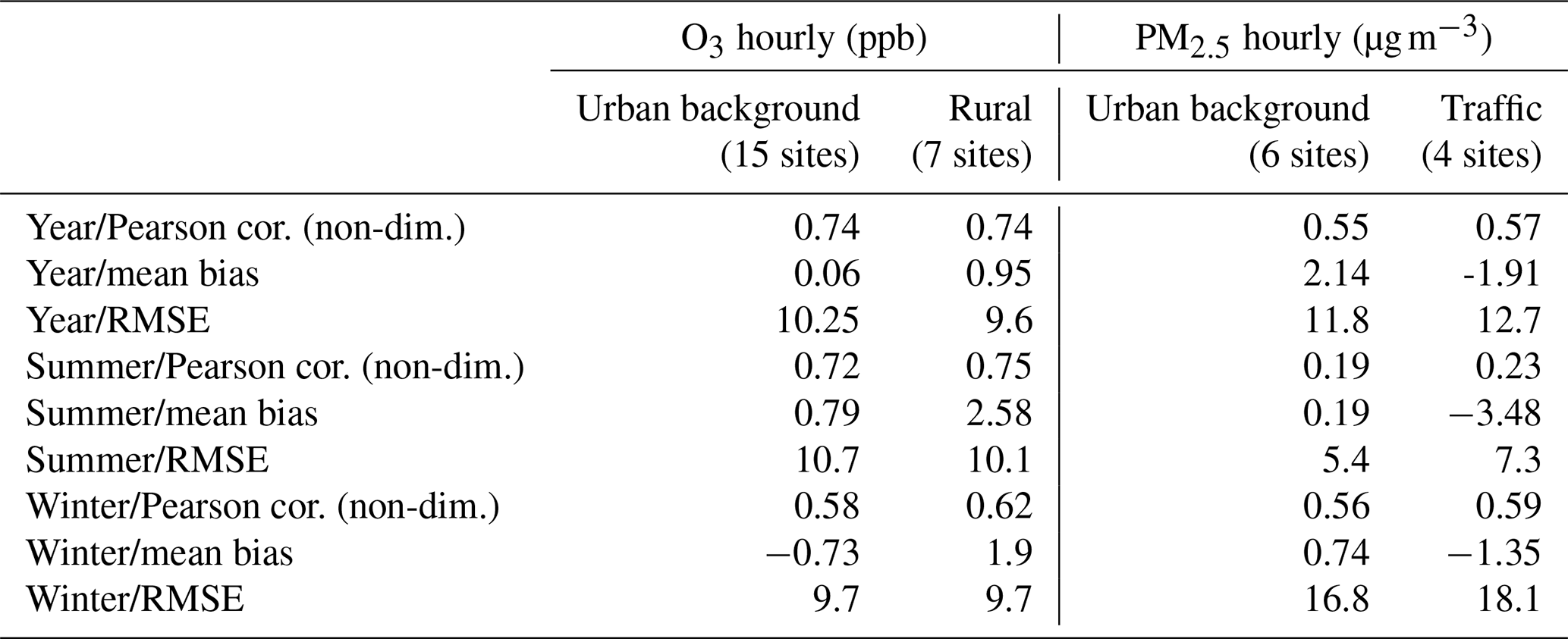
Table 1 summarizes the comparison between the 2017 simulation against measurements at all the available monitor sites of the AIRPARIF air-quality network. Urban monitoring sites are divided into two groups: traffic sites are located on the road network and have a relatively small spatial representativeness, whereas urban background stations are located away from the road network and their spatial representativeness spans over larger areas. Rural monitor sites are located outside the city and have the largest spatial representativeness. A good temporal correlation on an hourly basis is observed for ozone, especially for summer periods on both urban background and rural locations. The correlation is lower for the winter period. Afternoon ozone concentrations are underestimated over urban background stations, as also shown in Fig. 2. This is due to the model's horizontal resolution that is too coarse to spatially resolve the fast NO titration near high-emission sources. On the contrary, daytime ozone is slightly overestimated over rural locations; see Fig. S1 in the Supplement. In both urban background and rural locations, nighttime ozone is largely overestimated. The model keeps bringing ozone at the surface layer from the stratosphere, and ozone accumulates in the surface layer in the absence of local NO emissions and dry deposition that remove it during daytime.
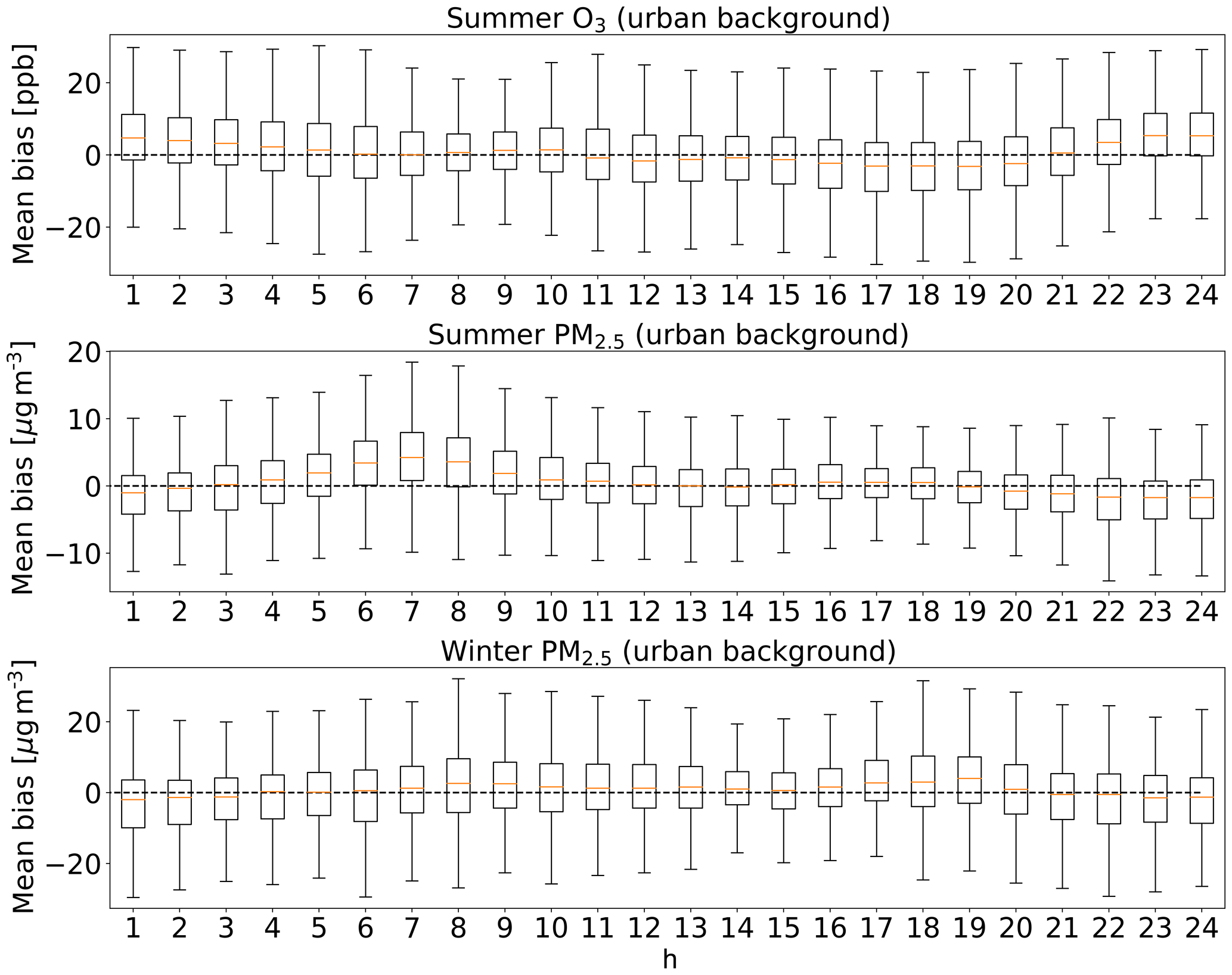
Figure 2Hourly mean bias of simulated surface O3 (summer) and PM2.5 (summer and winter) concentrations calculated during the year 2017 over 15 and 6 urban background monitor sites, respectively.
Temporal correlation, on an hourly basis, between simulated and observed PM2.5 concentrations is much better for winter than for summer. Pearson correlation over urban background sites drops from 0.56 for the winter period to 0.19 for summer. The CHIMERE model overestimates PM2.5 concentrations over urban sites and underestimates them over traffic stations (Table 1 and Fig. S2). Road transport is a major source of fine particles in urban areas. The 2 km×2 km horizontal resolution is insufficient to reproduce the high PM2.5 concentrations near these sources. Another possible reason for the model's underestimation of PM2.5 concentrations over traffic stations is a poor representation of secondary organic aerosol formation near traffic emissions. The distribution of the above statistics across sites is shown in Fig. S2 in the Supplement. As shown there, the underestimation of PM2.5 concentrations over traffic sites may be particularly high.
Globally, we assume that the CHIMERE model at 2 km×2 km resolution provides reliable O3 and PM2.5 background concentrations, being able to spatially differentiate the urban agglomeration from peri-urban and remote rural locations for PM2.5 (Fig. 3). The formation of well-structured ozone plumes over the rural area is also well represented, as shown in Fig. 3a, where a specific date/hour surface ozone concentration map is shown. The model is also capable of reproducing the diurnal cycle of ozone and PM2.5. Pollutant episodes induced by favourable meteorological conditions are also well-captured by the model, even though a trend to underestimate ozone peaks and overestimate PM2.5 peaks is observed. Based on this analysis, for the personal exposure calculation, we use simulated background O3 and PM2.5 concentrations from the CHIMERE model grid cell where the activity takes place. Over the road network, where we know that the 2 km×2 km CHIMERE model resolution is insufficient to reproduce the high PM2.5 concentration levels, we apply correction coefficients to increase modelled concentrations. This happens in two cases: the Boulevard Periphérique (road ring) and inside road tunnels (see Sect. 3.2.2). Therefore, no stochastic selection operates for the estimation of outdoor pollutant concentrations.

Figure 3Surface O3 (a, c) and PM2.5 (b, d) concentrations modelled with the CHIMERE chemistry–transport model. Maps on top show example of hourly averaged O3 concentration (a, c) and daily averaged PM2.5 concentration (b, d) for a specific hour/date. Maps on the bottom are annual averaged concentrations.
3.2 Infiltration of outdoor O3 and PM2.5 indoors
3.2.1 Dwellings, offices, and schools
Indoor pollutant concentration levels depend on indoor sources and on outdoor pollutants entering the building through natural or mechanical ventilation. As air flows through the envelope of the building, pollutants react with the surfaces over which they flow. Therefore, the actual flow indoors depends on the specific path that the air flow takes: permeability of the building shell, natural air entry, or ducts (Walker and Sherman, 2013). Other sinks of pollutants indoor are deposition on the indoor surfaces and chemical reactions with other indoor species. The relationship between these sources and sinks is expressed in Eq. (2) as in Walker et al. (2009):
Here,
-
CX,in and CX,out are the concentrations of pollutant X indoors and outdoors, respectively (µg m−3);
-
PX,I is the dimensionless penetration factor for the pollutant X through leak path i, i.e. the fraction of the pollutant in the infiltration air that passes through the building shell or air entrance;
-
Qin,i, Qout, and Qh are, respectively, the volume-normalized air flow rates into the building through path i, out of the building, and through the heating, ventilating, and air-conditioning equipment expressed in air changes per hour units (h−1);
-
η is the removal efficiency on the heating, ventilating, and air-conditioning equipment;
-
kd is the indoor deposition loss rate coefficient (h−1);
-
chemj is the concentration of the jth chemical species reacting with the X pollutant (µg m−3);
-
kj is the second-order rate constant for the j reaction (h−1);
-
SX is the time-varying indoor production rate (µg h−1); and
-
V is the volume (m3).
Several studies have measured indoor ∕ outdoor ratios for different building types and meteorological conditions in cities around the world for ozone (Collignan et al., 2012; Weschler, 2000) and airborne particles (Cyrys et al., 2004; Matson, 2005; Monn, 2001). Results show a strong dependence on the building usage (residence or office/school), the air tightness of the building, the ventilation system, and the proximity to atmospheric pollution sources. Ozone indoor ∕ outdoor (I ∕ O) ratios generally vary between 0.2 and 0.7 (Weschler, 2000), while for PM2.5, in the absence of indoor sources, they vary between 0.5 and 1 (Morawska and He, 2003).
To account for the variability in I ∕ O ratios due to these factors, we modelled ozone and fine airborne particles (PM2.5) I ∕ O ratios with the building ventilation model developed at the CSTB, called SIREN (Collignan et al., 2012). The differential equation (Eq. 2) is reformulated based on three assumptions: (i) no indoor sources for O3 and PM2.5; (ii) no chemical reactions with other atmospheric contaminants indoors; and (iii) initial concentration indoors is null. We conducted simulations for a typical dwelling and office/school.
To account for the variability of I ∕ O ratios due to air tightness and ventilation systems, we applied a classification of the building stock based on the construction date. This information integrates air tightness and ventilation system evolution based on the national thermal and ventilation regulations (ADEME, 2013), the evolution of the building stock as described in (INSEE, 2014), and the use of ventilation systems in French buildings (OQAI, 2006). Table 2 shows the applied parameterizations for the different usages and construction dates. The values of air tightness range from 2.5 m3 h−1 m−2 (representative of old leaky buildings) to 0.6 m3 h−1 m−2 (corresponding to new air-tight constructions). A sensitivity analysis with the SIREN model showed that the I ∕ O ratio for O3 decreases from 0.3 for the leaky building to 0.2 for the air-tight building and from 1 (air-tight building) to 0.8 (leaky building) for PM2.5. Based on the INSEE (2014) data, the percentages of dwellings constructed before 1974 in the non-thermally rehabilitated and thermally rehabilitated classes are 25 % and 75 %, respectively. No thermal rehabilitation is applied in offices and schools constructed before 1974. The air tightness and ventilation systems for offices and schools built after 2012 do not change but the proportion of buildings in this category increases with time.
Table 2Parameterization of the SIREN ventilation model depending on the construction date and the type of building, referring to the buildings' air tightness and the ventilation system.
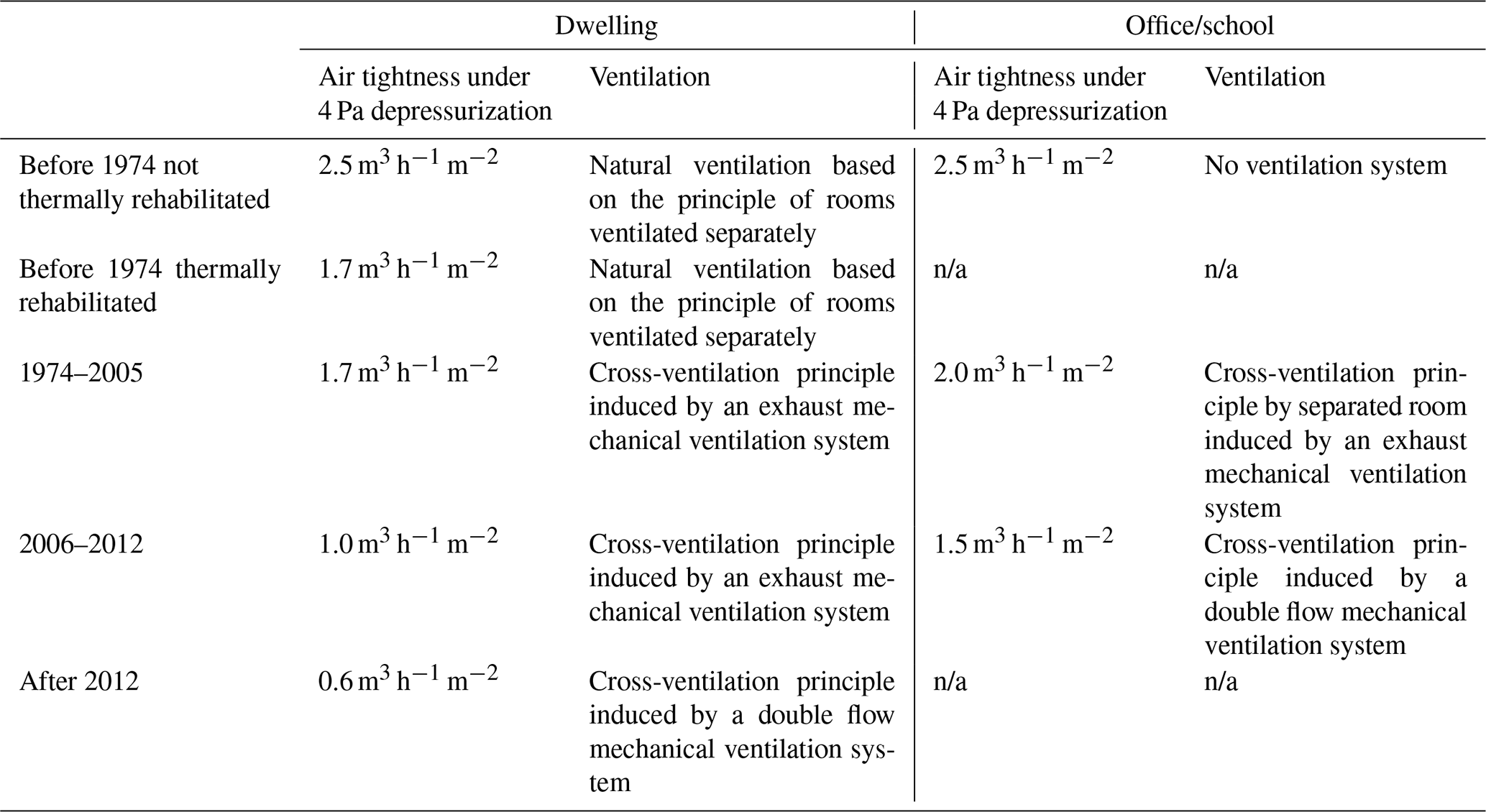
n/a – not applicable
Climatological conditions, temperature, pressure, and outdoor pollutant concentrations are simulated with atmospheric models (WRF for meteorology and CHIMERE for ozone and PM2.5 concentrations) at a 4×4 km2 horizontal resolution for a 10-year period from 1991 to 2000. Atmospheric fields are spatially averaged over the eight departments of the region. So, the atmospheric conditions database input for the SIREN model consists of 10-year period hourly data for the eight departments of the Île-de-France region.
For each Île-de-France department, eight SIREN simulations are conducted (five for dwellings and three for offices/schools) at a 3 min time step. The penetration factor is fixed to 0.8 through the building shell and 1 through air inlet based on the state of the art (Chen and Zhao, 2011; Monn, 2001; Stephens et al., 2012; Thatcher et al., 2003). Confronting numerical simulations with SIREN and I ∕ O ratio measurements, the deposition rate was fixed to 0.1 h−1. The SIREN model output consists of a decade-long database of I ∕ O ratios for ozone and PM2.5 at 3 min resolution for each of the eight Île-de-France departments, for five construction date classes for dwellings and three construction date classes for offices and schools. This database is further processed to provide seasonal I ∕ O ratios for each pollutant, building type, construction date, and geographical zone as shown in Fig. 4. Indoor ∕ outdoor ratios for the personal exposure calculation are drawn randomly from the corresponding seasonal distribution depending on the personal profile and month.
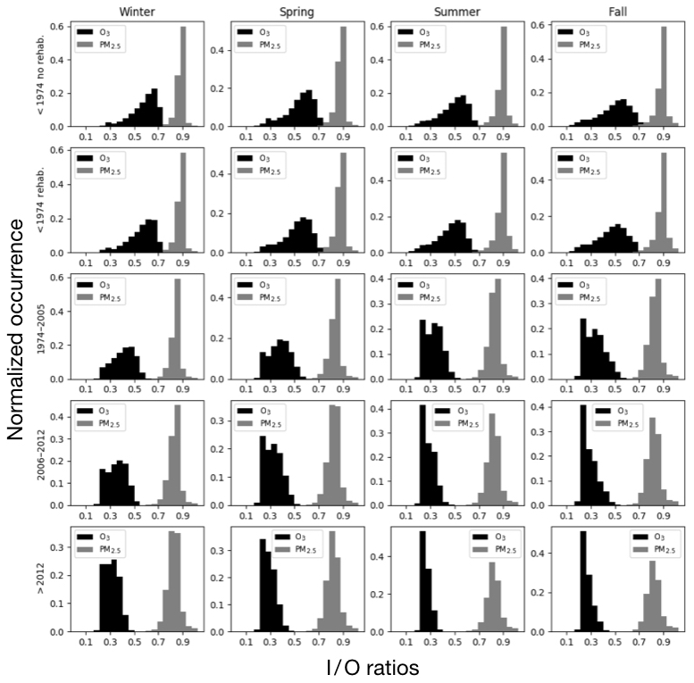
Figure 4O3 and PM2.5 indoor ∕ outdoor ratios modelled with the SIREN model for dwellings (unitless). The number of occurrences of the histogram is normalized over the size of the dataset.
3.2.2 Transportation
Ambient concentrations inside the principal transportation modes are deduced from outdoor concentrations by adjusting for indoor ∕ outdoor coefficients taken from a study dedicated to evaluating the pollutant levels to which the Île-de-France citizens are exposed while commuting to work and back during morning and evening rush hours (Delaunayet al., 2012). A significant number of contrasting situations is retained; 20 routes are chosen implementing the main modes of transport: car, bus, subway, tramway, cycling, and walking. Each route has been reproduced 30 times (15 round trips). The measurement campaign took place during the winter period of 2007 and 2008.
To define the indoor ∕ outdoor ratio for each journey in the model, we chose a random number within a uniform distribution between the minimum and maximum values obtained by the study of Delaunayet al. (2012). The extreme values of these distributions are shown in Table 3. For public transport, we distinguish between waiting on the platform and the journey. For the suburban train (RER), we distinguish between journeys inside the subway network in the Paris agglomeration and the rest of the network. For journeys in cars, we distinguish between the road network in the Paris agglomeration, the Boulevard Periphèrique (road ring), and the rest of the network (rural).
Table 3O3 and PM2.5 indoor ∕ outdoor ratios for the principal means of transportation.
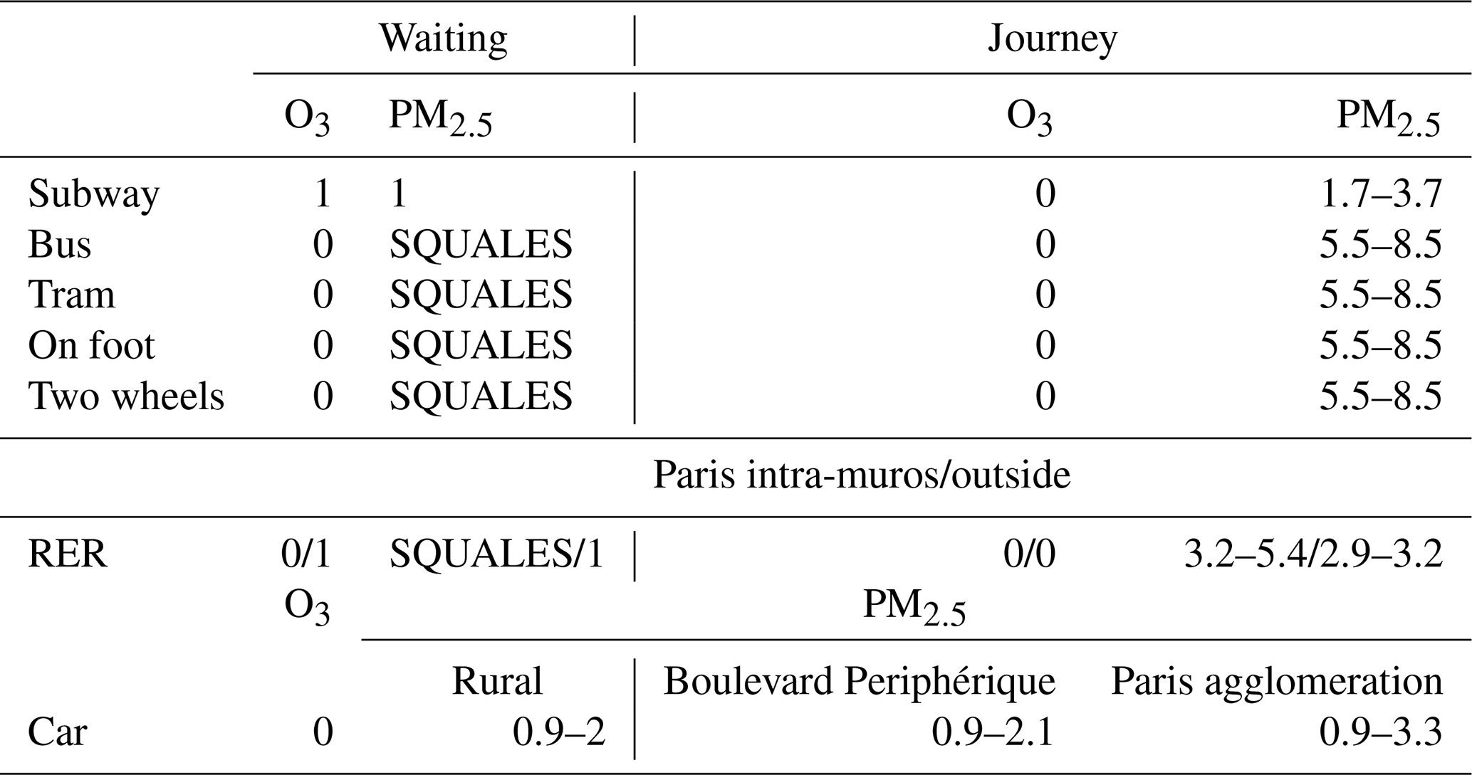
Several studies have shown that pollutant concentrations measured inside tunnels are several times higher than concentrations over the road but outside the tunnel. Orru et al. (2015) conducted a study to evaluate the health impact of the exposure to traffic exhaust inside road tunnels. Here, we apply a special adjustment for car journeys that cross tunnels. We assume that if the itinerary of an individual intersects a grid cell (2 km×2 km) containing a tunnel, there is a 20 % probability that the driver will pass through the tunnel. Due to lack of actual data, this number is assigned here in an arbitrary manner. Further investigation on traffic data could provide a more accurate estimate of this probability. Based on the measurement campaign described in AIRPARIF (2009), we assume that the PM2.5 concentration inside road tunnels is 2 times higher than the outdoor concentration (see also Sect. 2).
PM2.5 concentrations in the subway train tunnels are particularly high, especially for lines with rubber-tired railway vehicles. To keep a record of the air quality in the subway platforms, the RATP (Régie Autonome des Transports Parisiens) operates measurements on a 24 h basis at two metro stations and one RER platform (SQUALES). We used hourly on-platform measurements of the SQUALES network and outdoor concentration measurements from the AIRPARIF network for the entire year of 2013 to establish a diurnal cycle of the indoor ∕ outdoor ratio inside the subway platforms (Fig. 5). For the personal exposure calculation, we draw a random value from the hourly distributions of indoor ∕ outdoor ratios.
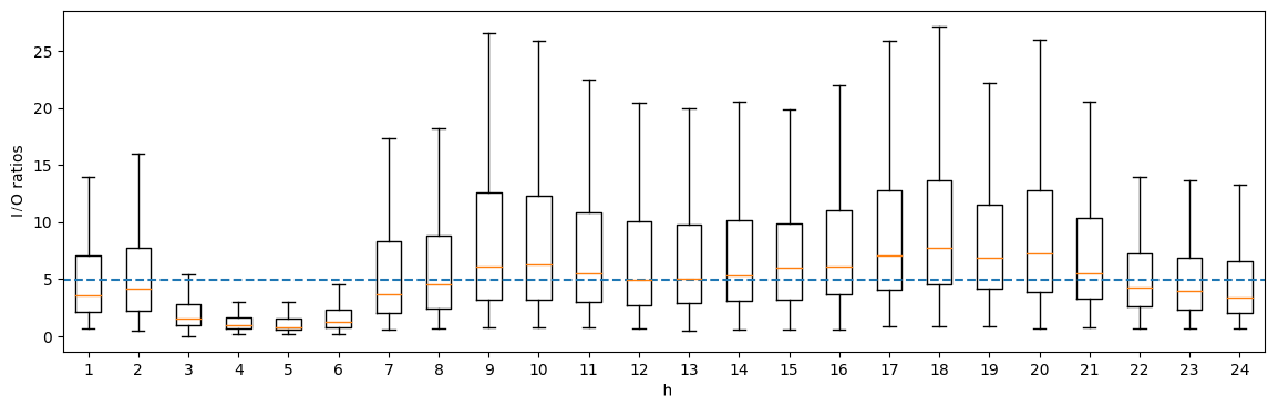
Figure 5Hourly distributions of indoor ∕ outdoor PM2.5 ratios for subway platforms issued from in-platform measurements of the SQUALES network and outdoor measurements of the AIRPARIF network. The blue line is the median I ∕ O ratio.
3.2.3 Other indoors
The SIREN model provides indoor ∕ outdoor ratios for dwellings, offices, and schools (Sect. 3.2.1). For other activities taking place indoors, such as entertainment and shopping, we use the same indoor ∕ outdoor ratios that SIREN predicts for offices and schools. For the personal exposure calculation, we draw random values for indoor ∕ outdoor ratios from the seasonal distributions. To decide whether shopping takes place indoors or outdoors, we used statistics from the IAURIF (2006) study, following which 14 % of the shopping activity in the Île-de-France region takes place outdoors. Entertainment other than exercise is assumed to always take place indoors. For exercise activities, we first chose the type of exercise activity (IAURIF, 2006) and then whether it takes place indoors or outdoors depending on the specific activity.
The methodological steps to obtain activity event sequences for the sample population are listed here:
-
select the population sample size that statistically reproduces essential demographics such as population of each administrative unit;
-
assign attributes to the members of the population such as age, gender, principal occupation, etc.; and
-
simulate the mobility of the population by matching the journeys of EGT (2010).
The Monte Carlo sampling method is used to randomly generate a dataset of simulated individuals based on these steps.
4.1 Generation of the sample population
The population data implemented in the model are public census data published by the INSEE (Institut Nationale de la Statistique et des Études Économiques). The current version of the model implements datasets for the year 2009. The administrative unit chosen for the current study is the commune. The Île-de-France region has 1300 communes and a population of 11 726 743. The most densely populated communes are located at the outer rings of the Paris agglomeration, followed by a second circle of high population density in the suburbs directly attached to the agglomeration. A third highly urbanized ring is distinguished before reaching the rural areas at the outskirts of the Île-de-France region (Fig. 6).
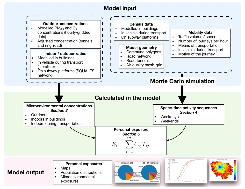
Figure 6Population density at the commune level in the Île-de-France region (left). Distribution of exposure factors in the sample population (right). Data source: census 2009 (INSEE).
The size of the sample population is fixed at 250 000 individuals (≈2 % of the actual population). A sensitivity analysis showed that further increasing this number does not significantly affect the results of the simulation (not shown). The first module of the model sequence assigns several demographic attributes to each member of the sample population. These attributes, referred to as exposure factors hereafter, remain unchanged throughout the simulation. The procedure consists of randomly selecting values from a distribution that matches the distribution of each attribute in the actual population of each commune. By repeating this process for each member of the sample population, we are sure to reproduce the distribution of the exposure factors in the simulated population.
The population is divided in four age groups. Five occupation classes are defined, and two possible contract types (full time or part time), corresponding to 9 or 5 h working days. Data on the construction date of the building of residence and work are also implemented to account for the infiltration of outdoor pollution indoors. The 10 exposure factors implemented in the model are listed below. The different possible values for each model parameter are shown.
-
Home commune: 1 out of 1300.
-
Gender: male, female.
-
Age group: <4, 4–24, 25–64, >64.
-
Occupation: day care, pupils/students, active employed, active unemployed, not active (retired, at home, other).
-
Contract: no contract, full time, part time.
-
Work area: same commune as residence, different commune in the same department, different commune in different Île-de-France department, outside Île-de-France or abroad.
-
Work commune: 1 out of 1300.
-
Means of transportation: no transportation, on foot, two wheels, car, public transport.
-
Construction date of residence: <1974 not rehabilitated, <1974 rehabilitated, 1974–2004, >2005.
-
Construction date of work place: <1974, 1974–2004, >2005.
A certain dependency exists between the exposure factors. For example, the professional occupation strongly depends on gender and age. To preserve the subpopulation variability in the sample population, the random sampling of the exposure factors operates on stratified data, where exposure factors are supposed to be homogeneous. First, we assigned the commune of residence and then the other attributes in the following order: gender, age group, principal occupation, and finally the kind of contract. Once these primary attributes were assigned, we then proceeded to the selection of the other, secondary characteristics. Working area is a function of the occupation and the commune of residence; the construction date of the buildings of residence depends on the commune, the gender, and the age group. For offices, general statistics are provided by Agence de l'Environnement et de la Maîtrise de l'Énergie (ADEME) for each Île-de-France department dividing offices in three age classes.
4.2 Modelling the activity sequences
The second module of the model compiles 24 h activity event sequences for each member of the sample population. Two diaries are compiled for each individual: one for weekdays and one for weekends. At each moment in time, people are either at home, engaged in an activity, or in transport. Eligible activities are the six motives for transport in the EGT (2010), namely work, professional affairs, school, market, recreation, or personal affairs. From this study, we deduce the number of journeys to take place at each hour in the region for each of the six aforementioned motives. Whenever an activity ends, or once every hour if the person is at home, the model checks whether the individual is about to move. Some restrictions are implemented, because not all individuals are eligible for all activities. For example, only certain age groups are eligible to go to day care or school, only employed people are bound to go to work, etc. Once these restrictions are implemented, people will move in order to match the proportions of journeys per motive at each hour. If the person is bound to move, a number of choices are made in the following order: (i) transportation mode; (ii) destination commune; (iii) travel distance; (iv) travel time; (v) activity duration (see also Fig. 7). For journeys to work and back, the INSEE provides a detailed dataset with the principal modes of transport. This information is part of the exposure factors assigned in the previous module (Sect. 4.1). The only stochastic choice here is for the two-wheel case, which has a 40 % and 60 % share between bicycles and motorcycles, respectively (EGT, 2010). For the rest of the journeys, we match the proportions of the transportation modes per motive and hour from the EGT (2010).
In some cases, the destination commune is known (the person goes to work, to study, or back home). For other cases, we only know whether the destination commune lies in the same department as the residence or in a different department. In this case, we first define the destination department based on data on the interdepartmental flows. Then we combine two pieces of information to assign the destination commune:
-
We use the data on the average distance travelled per means of transportation. We assume a straight line connecting the centroids of the communes. Several possible destination communes are selected based on the distance criterion.
-
We use the information on the destination commune for the journeys in EGT (2010) to assign a degree of attractiveness to the communes of the Île-de-France region for each motive.
To assign the distance of the journey, we distinguish between two cases. If the destination lies in a different commune, then the journey distance is assumed to be equal to the distance over a straight line connecting the centroids of the two communes. If the destination lies within the commune of the current location, then a stochastic choice is made for the travelled distance. We use statistics for the mean distance travelled per transportation means from the residents of the different departments. Depending on the transport mode, we assign a certain range around this average value and scale the limits to the commune size (radius of a circle with an area equal to the commune's area) and randomly choose a travel distance within this range.

To estimate the duration of the travel, we use two pieces of information at subcommunal scale. The first is the population density at 1×1 km2 resolution. Individuals are distributed over the 1×1 km2 resolution grid based on the population density. The second piece of information is the average speed and flow over the road segments of the traffic network. We assume a straight line linking the centres of the origin and destination cells of the 1×1 km2 grid and search for all grid cells that intersect this trajectory. The speed at which the grid cell is passed through is assigned stochastically based on the distribution of speeds over the road segments within the grid cell. We note here that it would be more accurate to base our selection on the flows over each road segment rather than the speed distribution, but the geometry of the problem would become too complex. Given the high resolution of the application, our insight is that this simplification is not bound to introduce significant errors to the transport model. The duration of the travel is then deduced from the distance and speed.
The final step is to define the duration of the activity. For children younger than 3 years old, we use statistics on the time spent at day care. In all other cases, we use statistics at department scale on the time spent by the population per activity.
A further distinction is whether the activity or transportation takes place indoors or outdoors. Certain activities may occur indoors or outdoors based on existing statistics (e.g. market and recreation). Possible means of transportation are on foot, two wheels (bicycle or motorcycle), car, bus, subway (metro), train (RER), and tramway. For public transportation, we distinguish between waiting time and travel time. For tramway, bus, and RER outside Paris, waiting takes place outdoors.
Figure 8 shows the results of the transport model. The diurnal patterns of the mobility of the population per motive are well reproduced. The model fails to reach the rush hour peaks, especially the morning peaks for work and school motives. It systematically underestimates the lunch hour peak. This is because the model does not implement secondary journeys, i.e. people leaving the workplace to go for lunch and then back to work. These remarks become clear when looking at the total number of journeys (bottom left of Fig. 8), where we also see that the model underestimates the number of journeys at all hours. However, the general picture of the simulation results is that the EGT (2010) data have been globally well implemented in the transport module.
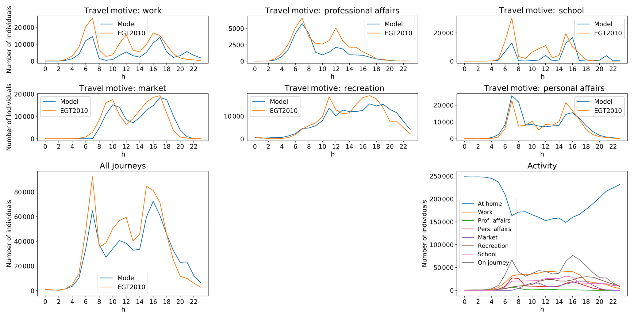
Figure 8Number of journeys per motive (first and second rows) and total number of journeys with all motives included (bottom left) at each hour. The number of individuals engaged in each activity at each hour of the day.
The transport module simulates the mobility of the population. When individuals reach their destination, they engage in the activity corresponding to the journey's motive. For activities other than travel, we assign a mean duration. Activity event sequences are simulated at 1 min temporal resolution. The ambient concentration at which people are exposed during the activity is the corresponding hour-averaged concentration modelled with the CHIMERE model at the grid cell where the activity takes place. In the case of travelling, the model simulates the trajectory of the journey. For car journeys, we use the mean hourly traffic flows on each segment of the road network to assign probabilities to each road and assign the route trajectories. The trajectory of the journey may intersect several CHIMERE grid cells. The corresponding outdoor concentrations are weighted by the time spent in each grid cell to estimate the aggregated exposure. Figure 8 (bottom right) shows the number of people engaged in each of the implemented activities at each hour of the simulation. Here, time activity is modelled based on available data for the region based on questionnaires. Modelling mobility patterns using smartphones with built-in GPS is an emerging trend in personal exposure assessment (Yu et al., 2019). Combining GPS-derived data on the trajectories of large number of individuals with information from questionnaires on the locations and activities of the population could help overcome a large part of the uncertainties relating to the time activity module developed in this study.
In this section, we highlight different possible applications of the exposure model. Each section looks at a different aspect of the model output as examples of its use in applications. The spatial distribution of exposure over the Île-de-France region is discussed in Sect. 5.1, the relative contribution of each microenvironment in the daily aggregated exposure is quantified in Sect. 5.2, the variability in exposure patterns across subpopulations is studied in Sect. 5.3, and the impact of considering (1) the infiltration of pollutants indoors and (2) the mobility of the population is illustrated in Sect. 5.4. Finally, in Sect. 5.5, we develop a 2050 horizon projection in the building stock of the Île-de-France region and quantify its impact in exposure to PM2.5 and ozone.
5.1 Exposure maps
Personal exposure may be spatially averaged over the communes to provide population exposure maps (Fig. 9). The annual averaged exposure to ozone is 3 times higher for the residents of the remote rural areas compared to the exposure of the Parisians. NO emitted by cars over the dense road network in the city of Paris reacts fast with O3 to form NO2. This explains the absence of O3 over the urban agglomeration. NO2 emitted in large amounts over Paris under the influence of sunshine and in the presence of volatile organic compounds forms O3 downwind, over the rural area (see also Fig. 3). We also note that the exposure to ozone is much lower than outdoor ozone concentration (30 and 15 ppb for the rural and urban areas, respectively; compare to maps in Fig. 3). This difference is due to the high amount of time people spent indoors, where ozone concentrations are close to zero (see also I ∕ O ratios for O3 Fig. 4).

Figure 9Annual averaged O3 and PM2.5 exposure maps. Personal exposure is spatially averaged among the residents of each commune.
The traffic network is a large source of PM2.5, which explains why exposure to PM2.5 is much higher in the Paris agglomeration than in the rural areas. Exposure to PM2.5 is much closer to concentration levels because I ∕ O ratios in buildings for PM2.5 are closer to 1 than those for O3. Annual mean PM2.5 concentrations are however lower than annual mean PM2.5 exposure (compare with concentration maps in Fig. 9). Even if indoor PM2.5 sources in buildings are not yet implemented in the model, and therefore concentrations in buildings are always lower than outdoor concentrations, PM2.5 concentrations in cars, subway trains, or on subway platforms are several times higher than outdoor concentrations (see Table 3). Even if the time spent in transport is relatively lower than the time spent inside buildings, concentrations there are so high that the daily aggregated exposure is higher than outdoor concentrations. The construction date of buildings also plays an important role, with older buildings (higher I ∕ O ratios) contributing to exposure at higher pollutant levels. Buildings in the Paris agglomeration are in general older than buildings outside of the city centre, and therefore indoor exposure to PM2.5 is higher for the residents of Paris.
5.2 Exposure in different microenvironments
The relative contribution of exposure in different microenvironments in the aggregated daily exposure depends on outdoor concentrations, the indoor ∕ outdoor coefficients if the activity takes place indoors, and the time spent in the microenvironment. For the active population (between 4 and 65 years old), residential exposure accounts for about 75 % of daily exposure to PM2.5 and almost 80 % of the aggregated exposure to O3 (Fig. 10), reflecting the large amount of time spent at home (see also bottom right panel in Fig. 8). Exposure at school represents the second largest part of total daily exposure to both pollutants (more than 10 %). Exposure outdoors represents a larger part of the total exposure for people between 24 and 65 years old (working population) than for children going to school (4–23 years old). For PM2.5 exposure in public, transportation and cars also have significant contributions.
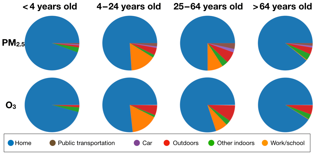
Figure 10Relative contribution of the different microenvironments in the aggregated daily exposure depending on the age group.
5.3 Exposure of subpopulation groups
Here, we study the impact of several exposure factors on personal exposure. Figure 11 shows the cumulative distribution of exposure over specific subpopulations. We identify the two factors that have the largest impact on personal exposure, namely the mode of transportation and the construction date of the building of residence. Both factors seem to strongly affect exposure to PM2.5 and ozone. People travelling by motorcycle or bicycle are exposed to the highest PM2.5 levels, while exposure in cars is the lowest. Overall, 10 % of the population using two wheels as a transportation mode is exposed to PM2.5 levels higher than the 25 µg m−3 EU target value related to human health. The percentage of the population exposed to PM2.5 levels above the EU target value drops to 5 % for people travelling by foot, 3 % for public transport, and 1 % for people travelling by car. The construction date of the home building also plays an important role in personal exposure. For both pollutants, exposure is higher for buildings constructed before 1974. A total of 100 % of the population living in buildings constructed after 2005 are exposed to PM2.5 levels below the EU target value, while 5 % of the population living in constructions before 1974 is exposed to levels above the EU target value.

Figure 11Cumulative distributions of exposure to PM2.5 (a, b) and O3 (c, d) for subpopulations distinguished by the transportation mode (a, c) and construction date of the building where they live (b, d).
5.4 Model sensitivity to population mobility and exposure indoors
Often, epidemiological methods estimate exposure metrics by modelling pollution concentrations at individual addresses. However, these models do not take into account exposure indoors nor population mobility. To provide insight into the exposure misclassification error due to this omission, we conducted several sensitivity studies. We calculated personal exposure to PM2.5 with and without accounting for the mobility of the population and exposure indoors as follows:
-
REF: the population stays at home and indoor concentrations are the same as outdoors.
-
+MOBILITY: the population moves but concentrations indoors are the same as outdoors.
-
+INDOORS BUILDINGS: the population stays at home and indoor ∕ outdoor coefficients for buildings are applied.
-
+INDOORS BUILDINGS & TRANSPORT: the population moves and indoor ∕ outdoor coefficients for both buildings and transportation are applied.
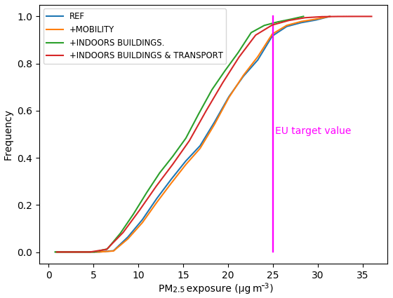
Figure 12Cumulative distributions of exposure to PM2.5 resulting for simulations integrating increasing levels of complexity in the input data.
Comparing the REF simulation with +MOBILITY shows that the mobility of the population within the region alone has a small negative impact on personal exposure (−1.5 % on the median). This may be explained by the fact that people spend most of their time indoors. We note here that Shekarrizfard et al. (2016) found an increase in personal exposure to NO2 that may be as high as +10 % in the Montreal metropolitan area when population mobility was accounted for compared to the simpler set-up where exposure at individual address was considered. This is explained by the difference in the air-quality models used in each study: a Gaussian dispersion model around each segment of the road network for the Shekarrizfard et al. (2016) study compared to a regional-scale CTM in our case. Accounting for residential exposure in the +INDOORS BUILDINGS simulation strongly affects personal exposure (−11 % difference with the REF in the median exposure). Accounting also for indoors exposure during transportation +INDOORS BUILDINGS & TRANSPORT leads to a 4.6 % increase in the median exposure compared to only accounting for residential exposure (+INDOORS BUILDINGS). PM2.5 concentrations during transportation are higher than outdoors, whereas concentrations in buildings are always lower than outdoors (no indoor sources in buildings). These results are comparable to the findings of Smith et al. (2016), who also estimated a decrease in personal exposure to PM2.5 in the London metropolitan area when population mobility and indoor exposure are accounted for. In the REF simulation, 5 % of the population is exposed to concentrations above the EU target value of 25 µg m−3, while in the complete implementation of indoor exposure only 2 % of the population is exposed to PM2.5 above this threshold (Fig. 12).

Figure 13Exposure to O3 (µg m−3) considering the actual building stock (a) and the 2050 horizon projection of the building stock (b).
5.5 2050 horizon projection of the building stock
Based on data on the evolution of the French building stock (INSEE, 2014) and the national thermal building regulation found in the 2013 report of the ADEME (ADEME, 2013), the CSTB developed a projection for the evolution of the building stock that is applied here for the 2050 horizon. To comply with thermal legislations and energy demand, buildings will tend to be more air tight and ventilation systems more efficient. This evolution in the building stock will also affect air quality in buildings and therefore human exposure to atmospheric contaminants.
Following this projection, in 2050 dwellings, offices and schools will still fall in the same categories presented in Table 2 but the proportions of buildings falling in each category will change due to demolition, new construction, and thermal rehabilitation. The projection developed here models the annual rate of change in the building stock as follows:
For dwellings (Eq. 3),
-
buildings belonging to the fifth class (construction date >2012) will increase;
-
buildings belonging to the first class (<1974 not rehabilitated) will decrease due to demolition and thermal rehabilitation; and
-
buildings belonging to the second class (<1974 rehabilitated) will increase due to thermal rehabilitation of buildings in the first class.
For offices and schools (Eq. 4),
-
buildings belonging to the third class (2006–2012) will increase; and
-
buildings belonging to the first class (<1974 not rehabilitated) will decrease due to demolition.
The projection is applied to the Île-de-France building stock, and we simulate personal exposure to quantify its impact. Due to new buildings being more air tight with a better control of air renewal using more efficient ventilation systems, even less ozone penetrates the building shell. The resulting reduction in annual average exposure to O3 is up to 14 % (Fig. 13). The change in annual averaged PM2.5 exposure is very small (not shown).
We developed a regional-scale model for personal exposure to PM2.5 and O3. The model uses simulated outdoor pollutant concentrations and models the infiltration of outdoor contaminants indoors in buildings with a ventilation mass-balance model. Three building types are considered: dwellings, schools, and offices. It also models population mobility inside the region considering the different possible transportation modes and adjusts for pollutant concentrations inside cars, buses, trams, subway trains, and regional trains. A special treatment for concentrations in subway platforms is applied considering online measurements on the platform and outdoors. An adjustment for ambient concentrations inside road tunnels is also applied from data from the literature. The model also uses data from the road traffic network to estimate the most probable trajectory for travel, as well as mean travel speed and duration.
We show that considering the population daily movement inside the region without accounting for the penetration of outdoor pollution indoors or indoor concentration during transportation has a small negative impact on annual averaged personal exposure. This is in contrast with the previous study of Shekarrizfard et al. (2016), who found an increase in exposure to NO2 in the Montreal metropolitan area when population mobility is accounted for. However, the two models are not directly comparable since they look at different pollutants at different timescales and use different air-quality models.
We show that accounting for the penetration of outdoor pollution indoors in buildings without considering population movement decreases annual averaged personal exposure by 11 % for PM2.5. This decrease stems only from the buildings' envelope acting as barrier to pollution infiltration indoors. When accounting also for population movement, annual averaged population exposure increases by 5 %, showing the importance of exposure during transportation. Even if travelling represents only a small portion of time, exposure to PM2.5 is too high and increases the daily burden of exposure. These results are in alignment with the previous study of Smith et al. (2016), who also found that personal exposure decreases in London when population mobility and exposure indoors are taken into account. The discrepancy in the magnitude of the decrease (−37 % in their case vs. −7 % in ours) may be due to the relatively coarse resolution of the outdoor concentration fields simulated with CHIMERE (2 km×2 km). However, if this resolution is not enough to solve concentration gradients at the proximity of local sources such as roads, it is capable to distinguish between urban, suburban, and rural concentrations. Most of the daily movement in the region crosses these boundaries (e.g. people living in the suburbs work in Paris,k and vice versa).
We conclude that both infiltration of pollutant indoors and population movement need to be considered to estimate the aggregated daily exposure. We note here that, so far, the model does not implement indoor sources of PM2.5 in buildings. We are aware that PM2.5 indoors may be several times higher than outdoor concentrations (as is the case during transport). However, in this version of the model, we were more interested to see how different building types and characteristics affect personal exposure independent of human activity that would drive indoor sources. The CSTB is working actively to develop parameterizations accounting for indoor emission sources of PM2.5 as well as their resuspension due to human activity.
Several applications of the model are presented. We first show the maps of exposure to O3 and PM2.5 over the region. The spatial distribution of the exposure field is very similar to the concentration one, showing the strong correlation of the aggregated exposure to outdoor concentration. However, we show that if we focus on specific subpopulation groups, such as people using bicycles or motorcycles systematically in their daily journeys, or people living in houses built before 1974, the upper percentiles of exposure are much higher than the general population. To study the impact of buildings' characteristics on personal exposure, we implemented a 2050 horizon projection of the building stock in the Île-de-France region. Following this projection, older buildings will be demolished or rehabilitated to comply with the thermal regulation and newer constructions will have modernized characteristics. The share of people living in the different building categories is modified to match this projection and personal exposure is simulated. The 2050 horizon personal exposure to O3 is decreased by as much as 14 % according to this projection.
This first version of the model is parameterized for data available for greater Paris. However, the input data required for the simulation are also available in other regions: census data, construction dates of buildings, and mobility data. We can therefore imagine that with small adjustments in the format, the model could be applied to other regions. In all applications presented here, outdoor concentration data are simulated with the CHIMERE model, and therefore the horizontal resolution is limited to the order of 1 km×1 km. However, this resolution limit is not inherent for the exposure model. If outdoor concentration fields at higher horizontal resolution were available from another dispersion model (e.g. Gaussian or Lagrangian), the exposure calculation would have run without any modification being necessary.
The source code of the EXPLUME v1.0 model as well as all necessary input data for the Île-de-France region (open source; see the acknowledgements) are available under https://doi.org/10.5281/zenodo.3352713 (Valari and Markakis, 2019).
The supplement related to this article is available online at: https://doi.org/10.5194/gmd-13-1075-2020-supplement.
MV coordinated the model development, ran the CHIMERE and EXPLUME simulations, and wrote the paper. KM did the major work of EXPLUME model development. EP and BC developed and ran the SIREN ventilation model for indoor/outdoor pollutant concentrations. OP provided data and expertise on anthropogenic emission fluxes over the Paris area.
The authors declare that they have no conflict of interest.
The authors acknowledge AIRPARIF for developing and providing the bottom-up anthropogenic emissions inventory used in this study. We also acknowledge RATP for maintaining the SQUALES network and publishing the data, as well as STIF, OMNIL, and DRIEA for rendering public the EGT2010 dataset. Finally, we acknowledge Raphael Lachieze Rey for his valuable help in the statistical modelling.
This work has received funding from the European Union's Horizon 2020 research and innovation programme under grant agreement no. 727816, as well as from ANSES, ADEME, BelSPO, UBA, and the Swedish EPA under the ERA-ENVHEALTH network grant agreement no. 219337. This work was performed using HPC resources from GENCI TGCC under grant no. A0050110274.
This paper was edited by Christoph Knote and reviewed by two anonymous referees.
ADEME: Les chiffres clés du bâtiment: énergie-environnement, Tech. Rep. Chiffes clés, Agence de l'Environnement et de la Maitrise de l'Energie, 2013. a, b
AIRPARIF: Quelle qualité de l'air en voiture pendant les trajets quotidiens domicile-travail, Tech. rep., AIRPARIF, available at: https://www.airparif.asso.fr/_pdf/publications/synthese_expovoituredomtra.pdf (last access: 29 July 2019), 2009. a
Anderson, H. R., Atkinson, R. W., Peacock, J., Marston, L., and Konstantinou, K.: Meta-analysis of time-series studies and panel studies of particulate matter (PM) and ozone (O3): report of a WHO task group, available at: https://apps.who.int/iris/handle/10665/107557 (last access: 28 July 2019), 2004. a
Appel, K. W., Gilliam, R. C., Pleim, J. E., Pouliot, G. A., Wong, D. C., Hogrefe, C., Roselle, S. J., and Mathur, R.: Improvements to the WRF-CMAQ modeling system for fine-scale air quality simulations, EM: Air And Waste Management Association's Magazine For Environmental Managers, 16–21, available at: https://cfpub.epa.gov/si/si_public_record_report.cfm?Lab=NERL&dirEntryId=288280 (last access: 28 July 2019), 2014. a
Atkinson, R. W., Mills, I. C., Walton, H. A., and Anderson, H. R.: Fine particle components and health – a systematic review and meta-analysis of epidemiological time series studies of daily mortality and hospital admissions, J. Expo. Sci. Env. Epid., 25, 208–214, https://doi.org/10.1038/jes.2014.63, 2015. a
Batterman, S., Ganguly, R., Isakov, V., Burke, J., Arunachalam, S., Snyder, M., Robins, T., and Lewis, T.: Dispersion Modeling of Traffic-Related Air Pollutant Exposures and Health Effects Among Children with Asthma in Detroit, Michigan, Transp. Res. Record, 2452, 105–112, https://doi.org/10.3141/2452-13, 2014. a
Beauchamp, M., Malherbe, L., and de Fouquet, C.: A pragmatic approach to estimate the number of days in exceedance of PM10 limit value, Atmos. Environ., 111, 79–93, https://doi.org/10.1016/j.atmosenv.2015.03.062, 2015. a
Beelen, R., Hoek, G., Vienneau, D., Eeftens, M., Dimakopoulou, K., Pedeli, X., Tsai, M.-Y., Künzli, N., Schikowski, T., Marcon, A., Eriksen, K. T., Raaschou-Nielsen, O., Stephanou, E., Patelarou, E., Lanki, T., Yli-Tuomi, T., Declercq, C., Falq, G., Stempfelet, M., Birk, M., Cyrys, J., von Klot, S., Nádor, G., Varró, M. J., Dėdelė, A., Gražulevičienė, R., Mölter, A., Lindley, S., Madsen, C., Cesaroni, G., Ranzi, A., Badaloni, C., Hoffmann, B., Nonnemacher, M., Krämer, U., Kuhlbusch, T., Cirach, M., de Nazelle, A., Nieuwenhuijsen, M., Bellander, T., Korek, M., Olsson, D., Strömgren, M., Dons, E., Jerrett, M., Fischer, P., Wang, M., Brunekreef, B., and de Hoogh, K.: Development of NO2 and NOx land use regression models for estimating air pollution exposure in 36 study areas in Europe – The ESCAPE project, Atmos. Environ., 72, 10–23, https://doi.org/10.1016/j.atmosenv.2013.02.037, 2013. a
Beevers, S. D., Kitwiroon, N., Williams, M. L., Kelly, F. J., Ross Anderson, H., and Carslaw, D. C.: Air pollution dispersion models for human exposure predictions in London, J. Expo. Sci. Env. Epid., 23, 647–653, https://doi.org/10.1038/jes.2013.6, 2013. a
Bell, M. L., Dominici, F., and Samet, J. M.: A meta-analysis of time-series studies of ozone and mortality with comparison to the national morbidity, mortality, and air pollution study, Epidemiology, 16, 436–445, 2005. a
Berchet, A., Zink, K., Muller, C., Oettl, D., Brunner, J., Emmenegger, L., and Brunner, D.: A cost-effective method for simulating city-wide air flow and pollutant dispersion at building resolving scale, Atmos. Environ., 158, 181–196, https://doi.org/10.1016/j.atmosenv.2017.03.030, 2017. a
Blair, A., Stewart, P., Lubin, J. H., and Forastiere, F.: Methodological issues regarding confounding and exposure misclassification in epidemiological studies of occupational exposures, Am. J. Ind. Med., 50, 199–207, https://doi.org/10.1002/ajim.20281, 2007. a
Cassee, F. R., Héroux, M.-E., Gerlofs-Nijland, M. E., and Kelly, F. J.: Particulate matter beyond mass: recent health evidence on the role of fractions, chemical constituents and sources of emission, Inhal. Toxicol., 25, 802–812, https://doi.org/10.3109/08958378.2013.850127, 013. a
Cattani, G., Gaeta, A., Di Menno di Bucchianico, A., De Santis, A., Gaddi, R., Cusano, M., Ancona, C., Badaloni, C., Forastiere, F., Gariazzo, C., Sozzi, R., Inglessis, M., Silibello, C., Salvatori, E., Manes, F., and Cesaroni, G.: Development of land-use regression models for exposure assessment to ultrafine particles in Rome, Italy, Atmos. Environ., 156, 52–60, https://doi.org/10.1016/j.atmosenv.2017.02.028, 2017. a
Chen, C. and Zhao, B.: Review of relationship between indoor and outdoor particles: I/O ratio, infiltration factor and penetration factor, Atmos. Environ., 45, 275–288, https://doi.org/10.1016/j.atmosenv.2010.09.048, 2011. a
Collignan, B., Lorkowski, C., and Améon, R.: Development of a methodology to characterize radon entry in dwellings, Build. Environ., 57, 176–183, https://doi.org/10.1016/j.buildenv.2012.05.002, 2012. a, b, c
Cyrys, J., Pitz, M., Bischof, W., Wichmann, H.-E., and Heinrich, J.: Relationship between indoor and outdoor levels of fine particle mass, particle number concentrations and black smoke under different ventilation conditions, J. Expo. Sci. Env. Epid., 14, 275–283, https://doi.org/10.1038/sj.jea.7500317, 2004. a
Delaunay, C., Goupil, G., Ravelomanantsoa, H., Person, A., Mazoue, S., and Morawski, F.: City dwellers exposure to atmospheric pollutants when commuting in Paris urban area, Pollution Atmospherique no. 215, 2012. a, b
Di, Q., Wang, Y., Zanobetti, A., Wang, Y., Koutrakis, P., Choirat, C., Dominici, F., and Schwartz, J. D.: Air Pollution and Mortality in the Medicare Population, New Engl. J. Med., 376, 2513–2522, https://doi.org/10.1056/NEJMoa1702747, 2017. a
Dias, D. and Tchepel, O.: Spatial and Temporal Dynamics in Air Pollution Exposure Assessment, Int. J. Env. Res. Pub. He., 15, 558, https://doi.org/10.3390/ijerph15030558, 2018. a
Edwards, J. K. and Keil, A. P.: Measurement Error and Environmental Epidemiology: A Policy Perspective, Current environmental health reports, 4, 79–88, https://doi.org/10.1007/s40572-017-0125-4, 2017. a
EEA: Air quality in Europe – 2019, Tech. Rep. 10/2019, available at: https://www.eea.europa.eu//publications/air-quality-in-europe-2019, last access: 4 November 2019. a
EGT: Enquête Globale Transport 2010-STIF-OMNIL-DRIEA, Tech. rep., 2010. a, b, c, d, e, f, g, h, i
Franklin, M., Vora, H., Avol, E., McConnell, R., Lurmann, F., Liu, F., Penfold, B., Berhane, K., Gilliland, F., and Gauderman, W. J.: Predictors of intra-community variation in air quality, J. Expo. Sci. Env. Epid., 22, 135–147, https://doi.org/10.1038/jes.2011.45, 2012. a
Georgopoulos, P. G., Wang, S.-W., Vyas, V. M., Sun, Q., Burke, J., Vedantham, R., McCurdy, T., and Ozkaynak, H.: A source-to-dose assessment of population exposures to fine PM and ozone in Philadelphia, PA, during a summer 1999 episode, J. Expo. Anal. Env. Epid., 15, 439–457, https://doi.org/10.1038/sj.jea.7500422, 2005. a
HEI: Traffic-Related Air Pollution: A Critical Review of the Literature on Emissions, Exposure, and Health Effects, Tech. Rep. Special Report 17, Health Effects Institute, Boston, MA, available at: https://www.healtheffects.org/publication/traffic-related-air-pollution-critical-review-literature-emissions-exposure-and-health ()last access: 28 July 2019, 2010. a
Hodas, N., Meng, Q., Lunden, M. M., Rich, D. Q., Özkaynak, H., Baxter, L. K., Zhang, Q., and Turpin, B. J.: Variability in the fraction of ambient fine particulate matter found indoors and observed heterogeneity in health effect estimates, J. Expo. Sci. Env. Epid., 22, 448–454, https://doi.org/10.1038/jes.2012.34, 2012. a
Hwang, Y. and Lee, K.: Contribution of microenvironments to personal exposures to PM10 and PM2.5 in summer and winter, Atmos. Environ., 175, 192–198, https://doi.org/10.1016/j.atmosenv.2017.12.009, 2018. a
IAURIF: Les déplacements pour achats, Analyse des comportements des franciliens en matière de déplacements pour achats, Tech. Rep., edited by: Delaporte, C. and Courel, J., Les cahiers de l'Enquête Globale de Transport. No 7, 2006. a, b
INSEE: Tableaux de l'économie francaise, Tech. rep., Institut Nationale de la statistique et des études économiques, Editions INSEE, 2014. a, b, c
Klepeis, N. E.: Modeling Human Exposure to Air Pollution, Human Exposure Analysis, CRC Press, Stanford, CA, 1–18, 2006. a, b, c
Korek, M. J., Bellander, T. D., Lind, T., Bottai, M., Eneroth, K. M., Caracciolo, B., Faire, U. H. d., Fratiglioni, L., Hilding, A., Leander, K., Magnusson, P. K. E., Pedersen, N. L., Östenson, C.-G., Pershagen, G., and Penell, J. C.: Traffic-related air pollution exposure and incidence of stroke in four cohorts from Stockholm, J. Expo. Sci. Env. Epid., 25, 517–523, https://doi.org/10.1038/jes.2015.22, 2015. a
Morawska, L. and He, C.: Relationship between indoor/outdoor concentrations of particles: a critical review, in: Proceedings of the 7th International Conference Healthy Buildings, National University of Singapore, Singapore, 7–11, 2003. a
Lim, S., Kim, J., Kim, T., Lee, K., Yang, W., Jun, S., and Yu, S.: Personal exposures to PM2.5 and their relationships with microenvironmental concentrations, Atmos. Environ., 47, 407–412, https://doi.org/10.1016/j.atmosenv.2011.10.043, 2012. a, b
Lipfert, F. W. and Wyzga, R. E.: On exposure and response relationships for health effects associated with exposure to vehicular traffic, J. Expo. Sci. Env. Epid., 18, 588–599, https://doi.org/10.1038/jes.2008.4, 2008. a
Mailler, S., Menut, L., Khvorostyanov, D., Valari, M., Couvidat, F., Siour, G., Turquety, S., Briant, R., Tuccella, P., Bessagnet, B., Colette, A., Létinois, L., Markakis, K., and Meleux, F.: CHIMERE-2017: from urban to hemispheric chemistry-transport modeling, Geosci. Model Dev., 10, 2397–2423, https://doi.org/10.5194/gmd-10-2397-2017, 2017. a, b
Matson, U.: Indoor and outdoor concentrations of ultrafine particles in some Scandinavian rural and urban areas, Sci. Total Environ., 343, 169–176, https://doi.org/10.1016/j.scitotenv.2004.10.002, 2005. a
McBride, S. J., Williams, R. W., and Creason, J.: Bayesian hierarchical modeling of personal exposure to particulate matter, Atmos. Environ., 41, 6143–6155, https://doi.org/10.1016/j.atmosenv.2007.04.005, 2007. a
Miranda, M. L., Edwards, S. E., Chang, H. H., and Auten, R. L.: Proximity to roadways and pregnancy outcomes, J. Expo. Sci. Env. Epid., 23, 32–38, https://doi.org/10.1038/jes.2012.78, 2013. a
Monn, C.: Exposure assessment of air pollutants: a review on spatial heterogeneity and indoor/outdoor/personal exposure to suspended particulate matter, nitrogen dioxide and ozone, Atmos. Environ., 35, 1–32, https://doi.org/10.1016/S1352-2310(00)00330-7, 2001. a, b
Morales Betancourt, R., Galvis, B., Rincón-Riveros, J. M., Rincón-Caro, M. A., Rodriguez-Valencia, A., and Sarmiento, O. L.: Personal exposure to air pollutants in a Bus Rapid Transit System: Impact of fleet age and emission standard, Atmos. Environ., 202, 117–127, https://doi.org/10.1016/j.atmosenv.2019.01.026, 2019. a
Olsson, D., Bråbäck, L., and Forsberg, B.: Air pollution exposure during pregnancy and infancy and childhood asthma, Eur. Respir. J., 44, p. 4237, 2014. a
Olstrup, H., Johansson, C., Forsberg, B., Tornevi, A., Ekebom, A., and Meister, K.: A Multi-Pollutant Air Quality Health Index (AQHI) Based on Short-Term Respiratory Effects in Stockholm, Sweden, Int. J. Env. Res. Pub. He., 16, 105, https://doi.org/10.3390/ijerph16010105, 2019a. a
Olstrup, H., Johansson, C., Forsberg, B., and Åström, C.: Association between Mortality and Short-Term Exposure to Particles, Ozone and Nitrogen Dioxide in Stockholm, Sweden, Int. J. Env. Res. Pub. He., 16, 1028, https://doi.org/10.3390/ijerph16061028, 2019b. a
OQAI: Campagne nationale Logements Etat de la qualité de l'air dans les gogements francais Rapport final, Tech. Rep. DDD/SB – 2006-57, Observatoire de la qualité de l'air interieur, edited by: Kirchner, S., Arenes, J.-F., Cochet, C., Derbez, M., Duboudin, C., Elias, P., Gregoire, A., Jédor, B., Lucas, J.-P., Pasquier, N., Pigneret, M., and Ramalho, O., 2006. a
Orru, H., Lövenheim, B., Johansson, C., and Forsberg, B.: Potential health impacts of changes in air pollution exposure associated with moving traffic into a road tunnel, J. Expo. Sci. Environ. Epidemiol., 25, 524–531, https://doi.org/10.1038/jes.2015.24, 2015. a
Pascal, M., Corso, M., Chanel, O., Declercq, C., Badaloni, C., Cesaroni, G., Henschel, S., Meister, K., Haluza, D., Martin-Olmedo, P., and Medina, S.: Assessing the public health impacts of urban air pollution in 25 European cities: Results of the Aphekom project, Sci. Total Environ., 449, 390–400, https://doi.org/10.1016/j.scitotenv.2013.01.077, 2013. a
Pascal, M., de Crouy Chanel, P., Wagner, V., Corso, M., Tillier, C., Bentayeb, M., Blanchard, M., Cochet, A., Pascal, L., Host, S., Goria, S., Le Tertre, A., Chatignoux, E., Ung, A., Beaudeau, P., and Medina, S.: The mortality impacts of fine particles in France, Sci. Total Environ., 571, 416–425, https://doi.org/10.1016/j.scitotenv.2016.06.213, 2016. a
Ryan, P. H. and LeMasters, G. K.: A review of land-use regression models for characterizing intraurban air pollution exposure, Inhal. Toxicol., 19, 127–133, https://doi.org/10.1080/08958370701495998, 2007. a
Sarnat, J. A., Wilson, W. E., Strand, M., Brook, J., Wyzga, R., and Lumley, T.: Panel discussion review: session 1–exposure assessment and related errors in air pollution epidemiologic studies, J. Expo. Sci. Env. Epid., 17, S75–82, https://doi.org/10.1038/sj.jes.7500621, 2007. a
Shekarrizfard, M., Faghih-Imani, A., and Hatzopoulou, M.: An examination of population exposure to traffic related air pollution: Comparing spatially and temporally resolved estimates against long-term average exposures at the home location, Environ. Res., 147, 435–444, https://doi.org/10.1016/j.envres.2016.02.039, 2016. a, b, c
Skamarock, C., Klemp, B., Dudhia, J., Gill, O., Barker, D., Duda, G., Huang, X.-y., Wang, W., and Powers, G.: A Description of the Advanced Research WRF Version 3, https://doi.org/10.5065/D68S4MVH, 2008. a
Smith, J. D., Mitsakou, C., Kitwiroon, N., Barratt, B. M., Walton, H. A., Taylor, J. G., Anderson, H. R., Kelly, F. J., and Beevers, S. D.: London Hybrid Exposure Model: Improving Human Exposure Estimates to NO2 and PM2.5 in an Urban Setting, Environ. Sci. Technol., 50, 11760–11768, https://doi.org/10.1021/acs.est.6b01817, 2016. a, b
Soares, J., Kousa, A., Kukkonen, J., Matilainen, L., Kangas, L., Kauhaniemi, M., Riikonen, K., Jalkanen, J.-P., Rasila, T., Hänninen, O., Koskentalo, T., Aarnio, M., Hendriks, C., and Karppinen, A.: Refinement of a model for evaluating the population exposure in an urban area, Geosci. Model Dev., 7, 1855–1872, https://doi.org/10.5194/gmd-7-1855-2014, 2014. a
Stephens, B., Gall, E. T., and Siegel, J. A.: Measuring the penetration of ambient ozone into residential buildings, Environ. Sci. Technol., 46, 929–936, https://doi.org/10.1021/es2028795, 2012. a
Sun, Q., Wang, W., Chen, C., Ban, J., Xu, D., Zhu, P., He, M. Z., and Li, T.: Acute effect of multiple ozone metrics on mortality by season in 34 Chinese counties in 2013–2015, J. Intern. Med., 283, 481–488, https://doi.org/10.1111/joim.12724, 2018. a
Thatcher, T. L., Lunden, M. M., Revzan, K. L., Sextro, R. G., and Brown, N. J.: A Concentration Rebound Method for Measuring Particle Penetration and Deposition in the Indoor Environment, Aerosol Sci. Tech., 37, 847–864, https://doi.org/10.1080/02786820300940, 2003. a
Valari, M. and Menut, L.: Transferring the heterogeneity of surface emissions to variability in pollutant concentrations over urban areas through a chemistry-transport model, Atmos. Environ., 44, 3229–3238, https://doi.org/10.1016/j.atmosenv.2010.06.001, 2010. a
Valari, M. and Markakis, K.: mvalari/EXPLUME: First release of EXPLUME (Version v1.0.0), Zenodo, https://doi.org/10.5281/zenodo.3352714, 2019. a
Valari, M., Menut, L., and Chatignoux, E.: Using a chemistry transport model to account for the spatial variability of exposure concentrations in epidemiologic air pollution studies, J. Air Waste Manage., 61, 164–179, 2011. a
Vizcaino, P. and Lavalle, C.: Development of European NO2 Land Use Regression Model for present and future exposure assessment: Implications for policy analysis, Environ. Pollut., 240, 140–154, https://doi.org/10.1016/j.envpol.2018.03.075, 2018. a
Walker, I., Sherman, M., and Nazaroff, W.: Ozone Reductions Using Residential Building Envelopes, Tech. Rep. LBNL-1563E, Lawrence Berkeley National Laboratory, california Institute for Energy and Environment, 2009. a
Walker, I. S. and Sherman, M. H.: Effect of ventilation strategies on residential ozone levels, Build. Environ., 59, 456–465, https://doi.org/10.1016/j.buildenv.2012.09.013, 2013. a
Weschler, C. J.: Ozone in Indoor Environments: Concentration and Chemistry, Indoor Air, 10, 269–288, https://doi.org/10.1034/j.1600-0668.2000.010004269.x, 2000. a, b
WHO: Review of evidence on health aspects of air pollution – REVIHAAP project: final technical report, available at: http://www.euro.who.int/en/health-topics/environment-and-health/air-quality/publications/2013/review-of-evidence-on-health-aspects-of-air-pollution-revihaap-project-final-technical-report (last access: 28 February 2020), 2013. a
Willers, S. M., Eriksson, C., Gidhagen, L., Nilsson, M. E., Pershagen, G., and Bellander, T.: Fine and coarse particulate air pollution in relation to respiratory health in Sweden, Eur. Respir. J., 42, 924–934, https://doi.org/10.1183/09031936.00088212, 2013. a
Williams, R. D. and Knibbs, L. D.: Daily personal exposure to black carbon: A pilot study, Atmos. Environ., 132, 296–299, https://doi.org/10.1016/j.atmosenv.2016.03.023, 2016. a
Xie, X., Semanjski, I., Gautama, S., Tsiligianni, E., Deligiannis, N., Rajan, R. T., Pasveer, F., and Philips, W.: A Review of Urban Air Pollution Monitoring and Exposure Assessment Methods, ISPRS Int. Geo-Inf., 6, 389, https://doi.org/10.3390/ijgi6120389, 2017. a
Xu, H., Bechle, M. J., Wang, M., Szpiro, A. A., Vedal, S., Bai, Y., and Marshall, J. D.: National PM2.5 and NO2 exposure models for China based on land use regression, satellite measurements, and universal kriging, Sci. Total Environ., 655, 423–433, https://doi.org/10.1016/j.scitotenv.2018.11.125, 2019a. a
Xu, H., Léon, J.-F., Liousse, C., Guinot, B., Yoboué, V., Akpo, A. B., Adon, J., Ho, K. F., Ho, S. S. H., Li, L., Gardrat, E., Shen, Z., and Cao, J.: Personal exposure to PM2.5 emitted from typical anthropogenic sources in southern West Africa: chemical characteristics and associated health risks, Atmos. Chem. Phys., 19, 6637–6657, https://doi.org/10.5194/acp-19-6637-2019, 2019b. a
Yu, X., Stuart, A. L., Liu, Y., Ivey, C. E., Russell, A. G., Kan, H., Henneman, L. R. F., Sarnat, S. E., Hasan, S., Sadmani, A., Yang, X., and Yu, H.: On the accuracy and potential of Google Maps location history data to characterize individual mobility for air pollution health studies, Environ. Pollut., 252, 924–930, https://doi.org/10.1016/j.envpol.2019.05.081, 2019. a