Volcanic ash forecast using ensemble-based data assimilation: an ensemble transform Kalman filter coupled with the FALL3D-7.2 model (ETKF–FALL3D version 1.0)

Quantitative volcanic ash cloud forecasts are prone to uncertainties coming from the source term quantification (e.g., the eruption strength or vertical distribution of the emitted particles), with consequent implications for an operational ash impact assessment. We present an ensemble-based data assimilation and forecast system for volcanic ash dispersal and deposition aimed at reducing uncertainties related to eruption source parameters. The FALL3D atmospheric dispersal model is coupled with the ensemble transform Kalman filter (ETKF) data assimilation technique by combining ash mass loading observations with ash dispersal simulations in order to obtain a better joint estimation of the 3-D ash concentration and source parameters. The ETKF–FALL3D data assimilation system is evaluated by performing observing system simulation experiments (OSSEs) in which synthetic observations of fine ash mass loadings are assimilated. The evaluation of the ETKF–FALL3D system, considering reference states of steady and time-varying eruption source parameters, shows that the assimilation process gives both better estimations of ash concentration and time-dependent optimized values of eruption source parameters. The joint estimation of concentrations and source parameters leads to a better analysis and forecast of the 3-D ash concentrations. The results show the potential of the methodology to improve volcanic ash cloud forecasts in operational contexts.

1 Introduction

Volcanic ash dispersal forecasts are routinely used to prevent aircraft encounters with volcanic ash clouds and to define flight rerouted trajectories, avoiding potentially contaminated airspace areas. In the aftermath of the 2010 Eyjafjallajökull volcanic eruption in Iceland, safety-based quantitative criteria for air traffic disruption were introduced, originally based on ash concentration thresholds and, more recently, on engine-ingested dosage (Clarkson et al., 2016). These scenarios involve the implementation of quantitative ash concentration forecasts, which require better model input constraints, particularly on ash emission rates and/or on model initialization. A large amount of scientific research has been conducted in recent years to achieve the following: (i) better quantify the amount of ash emitted, its vertical distribution across the column, and the related uncertainties; (ii) obtain data on the 3-D structure of ash clouds, particularly using ground, aircraft, and space-based instrumentation; (iii) improve model representation of the physical processes occurring within ash plumes and clouds; and (iv) transfer scientific outcomes into operations. However, despite the substantial advances in model formulation and initialization, it is estimated that, in operational contexts, forecasted ash concentrations can still have an uncertainty as large as 1 order of magnitude (e.g., IVATF, 2011).

Epistemic uncertainties in ash dispersal forecasts may have different origins, including the following: (i) uncertainties in the source term (i.e., eruption column height, mass eruption rate, particle grain size distribution); (ii) uncertainties in the atmospheric model driving dispersal simulations (e.g., wind velocity and direction, small-scale turbulence intensity, atmospheric temperature, and humidity); and (iii) uncertainties in model parameterizations of the physical processes occurring both in the eruptive column and during subsequent passive transport (e.g., ash settling and removal processes, particle aggregation, interaction with meteorological clouds, etc.). In addition to these, aleatoric uncertainties always exist regarding the future evolution of the eruption source parameters (ESPs) when an eruption is ongoing at the time of running a forecast. Several studies (e.g., Zehner, 2010; Kristiansen et al., 2012) have concluded that the main source of epistemic uncertainty in ash dispersal forecasts comes from ESPs that very often are not well constrained in real time.

Inverse modeling and, in particular, data assimilation methods are techniques that can be used to estimate the state of dynamical systems based on partial and noisy observations. In a broad sense, these techniques build on continuous or quasi-continuous observations to produce model initial conditions (analyses) that can be used to better predict the future state, taking into account uncertainties in observations and model formulation. Data assimilation methods have been successfully applied to the estimation of the state of the ocean or the atmosphere (e.g., Kalnay, 2003; Carrassi et al., 2018) as well as for the optimization of uncertain model parameters (e.g., Ruiz et al., 2013). More recently, applications have been extended to atmospheric constituents (e.g., Bocquet et al., 2010; Hutchinson et al., 2017), including ash dispersion models with the purpose of estimating the 3-D distribution of ash concentrations to be used as initial conditions for forecasts. Surprisingly, examples of the application of data assimilation techniques to volcanic ash dispersion are scarce and still mainly limited to a research level. For example, Wilkins et al. (2015) implemented a data insertion methodology to improve the initial conditions of ash concentrations based on satellite estimations of ash mass loadings in a Lagrangian dispersion model. Fu et al. (2015, 2017a) applied an ensemble Kalman filter technique to the estimation of ash concentrations in an Eulerian dispersion model based on flight concentration measurements and satellite estimations using idealized experiments and real observations. Their results showed that both observational sets (flight measurements and satellite mass loads) reduced forecast errors, which in their particular case were attributed to a wrong model representation of ash sedimentation processes. One important issue when using satellite estimates of ash mass loadings is that observations only provide a 2-D distribution of ash mass, while models usually require the vertical profile of ash concentrations. Fu et al. (2017b) presented a modified approach for comparison between models and observations in the context of the ensemble Kalman filter that tries to deal with this limitation.

Uncertainties in the source parameters can be circumvented in part by using inverse modeling techniques for the optimization of these parameters. Eckhardt et al. (2008) implemented a source parameter optimization approach based on the definition of a cost function that measures the departure of ash concentrations from observed values and the departure of the estimated parameters from their a priori values. This allowed for the reconstruction of the full emission profile using data from different sensors. Stohl et al. (2011), Kristiansen et al. (2012), Denlinger et al. (2012), Pelley et al. (2015), and Steensen et al. (2017) discussed further developments and evaluations of the proposed approach. In particular, Pelley et al. (2015) describe the operational implementation of this algorithm at the London Volcanic Ash Advisory Centre (VAAC). In Chai et al. (2017), the optimal parameters are found using a quasi-Newtonian minimization approach of a similar cost function, and Lu et al. (2016) use a similar approach in the context of an Eulerian model. Finally, Zidikheri et al. (2017a, b) presented an optimization algorithm based on a systematic search of the optimal parameter values for both qualitative and quantitative ash forecasts and evaluated the performance of the technique for different cases, showing a positive impact on forecast quality. Wang et al. (2017) perform idealized experiments in which a particle filter and an expectation maximization algorithm are used for the estimation of ash source parameters, obtaining promising results.

The goal of this paper is to contribute to the development of data assimilation methods to improve quantitative ash dispersion forecasts. To this end, we propose an ensemble-based data assimilation system for volcanic ash combining an ensemble transform Kalman filter (ETKF) (Ott et al., 2004; Hunt et al., 2007) and the FALL3D ash dispersal model (Costa et al., 2006; Folch et al., 2009), named ETKF–FALL3D. This system produces a joint estimation of 3-D ash concentration and critical ESPs that can improve the performance of classical ash dispersion forecast strategies. This paper presents a first analysis of the ETKF–FALL3D system using different observing system simulation experiments (OSSEs) in which synthetic observations of ash column mass loadings are simulated and assimilated. The system is evaluated under constant and time-dependent ESPs, and the sensitivity of the system performance to parameter uncertainty, ensemble size, and observation uncertainty is explored and discussed. Additionally, some impacts of the Gaussian assumptions underlying the ensemble Kalman filter in the present case are discussed. A description of the methodology is presented in Sect. 2, the experimental setup of the sensitivity experiments is described in Sect. 3, the results are discussed in Sect. 4, and the final conclusions are outlined in Sect. 5.

2 Methodology

2.1 The FALL3D model

FALL3D is an Eulerian atmospheric dispersal model that solves the advection–diffusion–sedimentation equation for a set of particle classes (bins), each characterized by a particle size, density, and shape factor. Given an eruption source term and meteorological variables, FALL3D solves the 4-D ash concentration for each particle class, from which the total and the fine ash column mass loadings are diagnosed by performing a vertical integration. The meteorological fields must be furnished offline by a numerical weather prediction (NWP) model forecast or from a reanalysis dataset. The source term determines the amount of tephra injected to the atmosphere, its vertical distribution along the eruption column, and the fraction of mass associated with each particle bin. This term can be parameterized using different schemes available in the model for the mass eruption rate (MER) (e.g., Mastin et al., 2009; Degruyter and Bonadonna, 2012; Woodhouse et al., 2013) and the vertical mass distribution (e.g., Pfeiffer et al., 2005; Folch et al., 2016). For simplicity and without loss of generality, we will assume here a MER given by the Mastin et al. (2009) scheme, which depends on the fourth power of the top height of the eruptive column and does not account for wind effects, and a Suzuki vertical mass distribution (Pfeiffer et al., 2005) that is an empirical vertical ash mass eruption rate distribution that assumes no interactions with the surrounding atmosphere (e.g., the effects of wind shear or stratification upon the eruptive column); it is also assumed that the shape of the vertical flow rate is the same for all particle sizes and is given by

$$\begin{array}{}\text{(1)}& S\left(z\right)={\left(\mathrm{1}-{\displaystyle \frac{z}{h}}\exp \left[A\left({\displaystyle \frac{z}{h}}-\mathrm{1}\right)\right]\right)}^{\mathit{\lambda }},\end{array}$$

where S(z) is the mass eruption rate distribution function, z is the altitude above the vent, h is the top height of the eruptive column, and A and λ are two dimensionless parameters. Figure 1 shows the sensitivity of the vertical emission profile to different values of h and A. It is important to recall that h not only controls the maximum height of the eruptive column, but also the total mass emitted (Fig. 1a). Parameter A does not modify the total amount of mass being emitted but significantly affects the level at which the maximum emission takes place (Fig. 1b), which can significantly affect the posterior evolution of the ash plume, particularly for cases in which there is strong vertical wind shear. The parameter λ is a measure of how concentrated the emission is around the maximum (not shown). A previous sensitivity test (Osores, 2018) has shown that the two FALL3D model parameters that most affect the model results are the eruption column height h and the parameter A in the Suzuki distribution. For this reason, these two parameters will be used in the following sections to define the ETKF–FALL3D system experiments. The sensitivity of the FALL3D model to these parameters in terms of the deposit has been documented by, e.g., Scollo et al. (2008).

Figure 1 Vertical mass distribution for different (a) eruptive column top heights and (b) A Suzuki parameters.

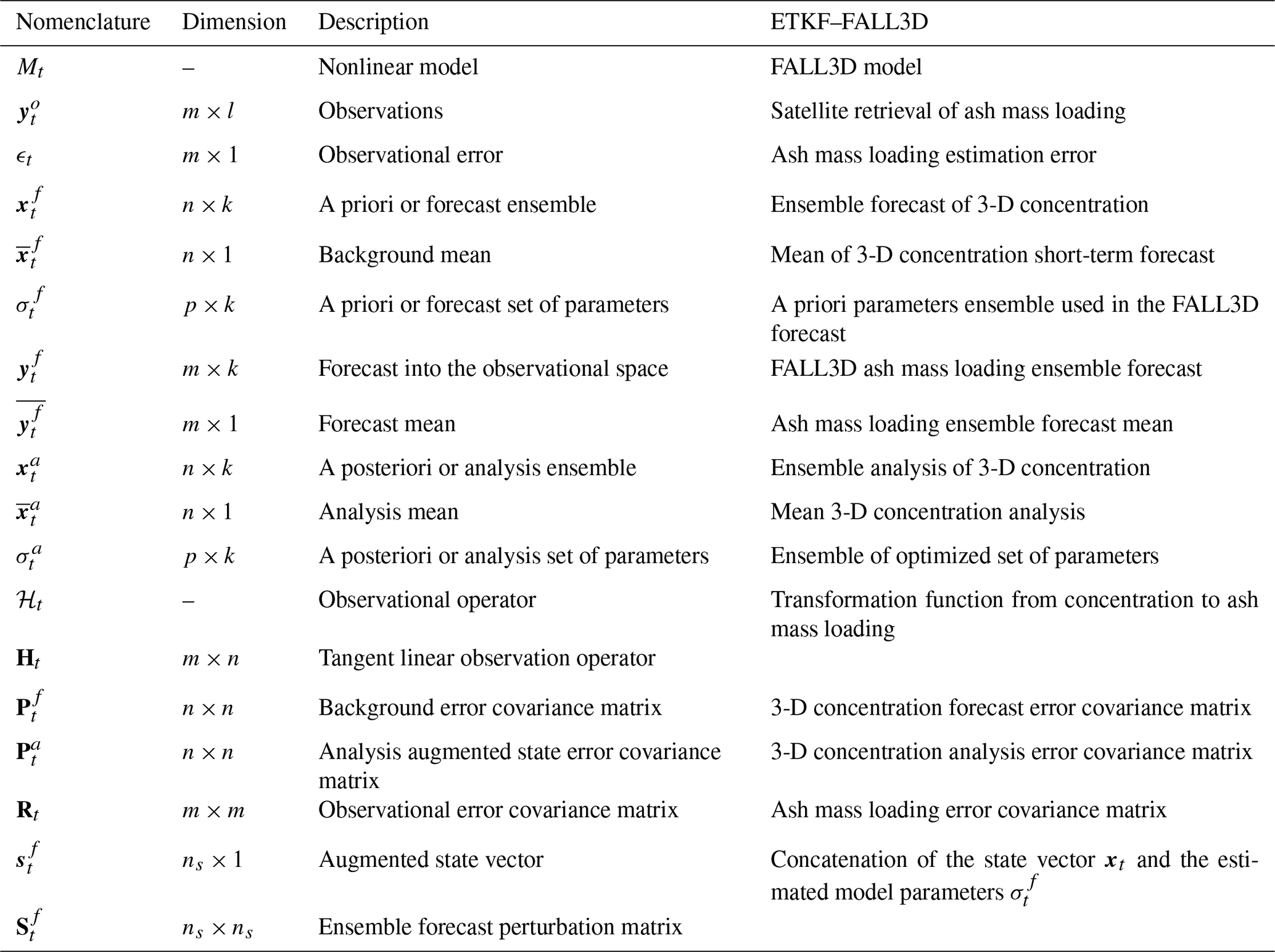
Table 1 Summary of the notation used in the paper, with the nomenclature for the ETKF method and its correspondence to the experiments discussed in this work. Here, n is the total number of grid points times the number of particle classes in the FALL3D model, m is the number of observations at time t, p is the number of parameters, and k is the number of ensemble members.

2.2 The ETKF–FALL3D system

In operational applications, data assimilation is implemented sequentially to provide an estimation of the state of the system at a series of times in the so-called “data assimilation cycle”. Each data assimilation cycle consists of two steps: a first step in which the numerical model is used to provide an a priori estimation or forecast of the state of the system and its uncertainty, followed by a second step in which the prior estimation is combined with observations (which are also considered uncertain) to obtain a posterior estimation or analysis. These two steps are repeated sequentially in order to propagate forward in time information from past observations.

Let us assume that the state of a system at time t is represented by a state vector x_t that, in our particular case, consists of the values of ash concentration at each model grid point and for each particle class. In other words, x_t is a column vector with n elements, n being the total number of state variables in the FALL3D model (i.e., the total number of grid points times the number of particle bins). For parameter estimation, model parameters θ, e.g., those defining the characteristics of the source term, are also considered part of the state of the system and are thus assumed uncertain. For the sake of simplicity, we limit the FALL3D source term parameters to the eruption column height h and the A-Suzuki parameter, but the methodology that follows can easily be extended to any other set of model input parameters. The augmented state vector s_t at time t is defined as the concatenation of the state vector x_t and the (time-dependent) estimated model parameters θ; that is, ${\mathit{s}}_t=[x_t,{\mathit{\theta }}_t]$ is a column vector with $n_s=n+\mathrm{2}$ elements.

In the ensemble Kalman filter the time-dependent uncertainty in the state variables and parameters is estimated using a Monte Carlo approach through an ensemble of augmented states. Let us assume that we start at time t−1 with an ensemble of initial conditions and model parameters. Then, our forecast of the state of the system at time t is obtained by integrating in time the FALL3D model for each ensemble member:

$$\begin{array}{}\text{(2)}& {\mathit{s}}_t^{f\left(i\right)}=M_t\left({\mathit{x}}_{t-\mathrm{1}}^{a\left(i\right)},{\mathit{\theta }}_{t-\mathrm{1}}^{a\left(i\right)}\right),\end{array}$$

where M_t represents the FALL3D model operator, which integrates the model in time for the ith ensemble member starting from the ith initial conditions (analysis) ${\mathit{x}}_{t-\mathrm{1}}^a$ and fixes the model parameters to ${\mathit{\theta }}_{t-\mathrm{1}}^a$ during the time integration interval. Note that a persistence model is assumed for the model parameters (i.e., ${\mathit{\theta }}_t^f={\mathit{\theta }}_{t-\mathrm{1}}^a$) since no information about its variations is available yet during the forecast. Following the assumptions of the ensemble Kalman filter, the joint a priori probability distribution of the augmented state at time t is assumed Gaussian, with a mean and a covariance matrix estimated from the ensemble of forecasts:

$$\begin{array}{}\text{(3)}& \stackrel{\mathrm{‾}}{{\mathit{s}}_t^f}=k^{-\mathrm{1}}\sum _{i=\mathrm{1}}^k{\mathit{s}}_t^{f\left(i\right)},\end{array}$$

$$\begin{array}{}\text{(4)}& {\mathbf{P}}_t^f=(k-\mathrm{1}{)}^{-\mathrm{1}}{\mathbf{S}}_t^f{{\mathbf{S}}_t^f}^T,\end{array}$$

where $\stackrel{\mathrm{‾}}{{\mathit{s}}_t^f}$ is the ensemble forecast mean, ${\mathbf{P}}_t^f$ is the ensemble forecast covariance matrix (a square matrix of dimension n_s×n_s), and ${\mathbf{S}}_t^f$ is the ensemble forecast perturbation matrix whose ith column is computed as ${\mathbf{S}}_t^{f\left(i\right)}={\mathbf{s}}_t^{f\left(i\right)}-\stackrel{\mathrm{‾}}{{\mathbf{s}}_t^{f\left(i\right)}}$.

Figure 2 ETKF–FALL3D data assimilation system scheme for volcanic ash.

Note that the integration of the ensemble in time propagates the uncertainty on the initial conditions and parameters at time t−1 into the future in order to provide a time-dependent estimation of the forecast uncertainty. This is a key feature that makes these methods particularly appealing for the estimation of uncertain model parameters (e.g., Aksoy et al., 2006; Ruiz et al., 2013) and for an accurate quantification of concentration. At the analysis step a set of observations is available that is related to the true state of the system by the following expression:

$$\begin{array}{}\text{(5)}& {\mathit{y}}_t=\mathcal{H}\left({\mathit{x}}_t^{\text{true}}\right)+{\mathit{ϵ}}_t,\end{array}$$

where y_t is an m-sized column vector containing the value of the m observations at time t, and x^true is the true model state (assumed to be unknown). ℋ is a (usually nonlinear) transformation that maps the state variables (i.e., ash concentrations for different particle sizes) into the observed quantities (e.g., cloud column mass load), and the vector ϵ represents the error in the observations. This error is typically assumed to be a zero-mean Gaussian random variable with covariance matrix R (dimensions of m×m). The errors in the observations are assumed to be uncorrelated in time and independent of the state of the system. Under these assumptions, the information provided by the forecast and the observations can be combined to obtain an estimation of the augmented state that minimizes the root mean square error (RMSE) with respect to the unknown truth (e.g., Kalnay, 2003; Carrassi et al., 2018):

$$\begin{array}{}\text{(6)}& \stackrel{\mathrm{‾}}{{\mathit{s}}_t^a}=\stackrel{\mathrm{‾}}{{\mathit{s}}_t^f}+{\mathbf{P}}_t^f{\mathbf{H}}_t^T({\mathbf{H}}_t{\mathbf{P}}_t^f{\mathbf{H}}_t^T+\mathbf{R}{)}^{-\mathrm{1}}\left({\mathit{y}}_t^f-\mathcal{H}\left({\mathit{x}}_t^f\right)\right),\end{array}$$

where $\stackrel{\mathrm{‾}}{{\mathit{s}}_t^a}$ is the a posteriori estimation of the augmented state (i.e., the analysis), and H_t is the tangent linear of the observation operator. The factor ${\mathbf{P}}_t^f{\mathbf{H}}_t^T({\mathbf{H}}_t{\mathbf{P}}_t^f{\mathbf{H}}_t^T+\mathbf{R}{)}^{-\mathrm{1}}$ is usually referred to as the Kalman gain. The Kalman filter equations also provide a way to estimate the uncertainty of the analysis. After the assimilation of the observations, the augmented state covariance matrix is updated to

$$\begin{array}{}\text{(7)}& {\mathbf{P}}_t^a=(\mathbf{I}-{\mathbf{KH}}_t){\mathbf{P}}_t^f,\end{array}$$

where ${\mathbf{P}}_t^a$ is the posterior or analysis-augmented state covariance matrix. Note that Eqs. (6) and (7) can be used to obtain an ensemble of analyses for the state variables, and the parameters whose ensemble mean is equal to $\stackrel{\mathrm{‾}}{{\mathit{s}}_t^f}$ and the perturbations are sampled from a Gaussian distribution with zero mean and covariance matrix equal to ${\mathbf{P}}_t^a$. These equations can be difficult to solve explicitly for high-dimensional systems due to the large size of P_t and R_t, but several methods have been proposed to address this issue and to implement the ensemble Kalman filter in high-dimensional systems. In the present work, we use the ETKF approach, which solves the ensemble Kalman filter equations in a subspace defined by the ensemble members. Details about the equation that arises from this particular implementation can be found in Hunt et al. (2007), but a summary is given in Appendix A. Table 1 also presents a summary of the notation and dimensions associated with the different quantities previously discussed. One of the main advantages of this approach is that finding the analysis ensemble mean requires inverting a k×k matrix, which is significantly cheaper than inverting the n×n matrix for the case in which k≪n (which is usually the case for high-dimensional applications of the filter).

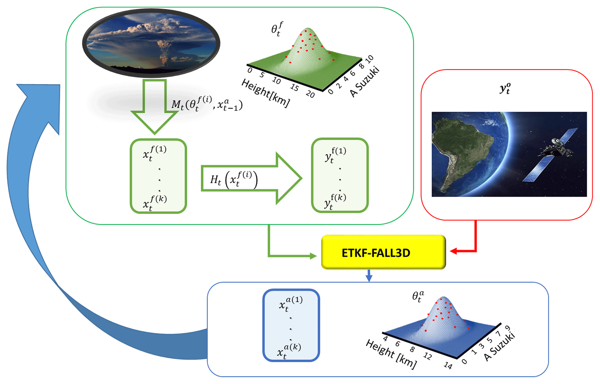
The process is schematically shown in Fig. 2. The cycle starts with an estimation of the mean parameters; assuming they have a Gaussian distribution, k random samples are taken. Each parameter sample is used in one of the ensemble members integrated with the dispersion model. When an observation is available, it is combined with the ensemble forecasts using the ETKF equations. From this combination an ensemble of analysis is obtained with a set of optimized parameters that also has a Gaussian distribution. Then the next cycle starts from the ensemble of analysis and the set of optimized parameters to produce a new ensemble forecast. When a new observation is available, the assimilation method is applied, and the cycle continues.

3 ETKF–FALL3D experimental setup

To explore the capability of the ETKF–FALL3D system we use an OSSE approach, in which a long model integration is performed and regarded as the true evolution of the ash cloud. This model integration will be referred to as the nature run. Observations are simulated from the nature run and then assimilated with the ETKF–FALL3D system. The June 2011 Puyehue-Cordón Caulle eruption (Osores et al., 2012; Collini et al., 2013) has been selected for the generation of the nature run.

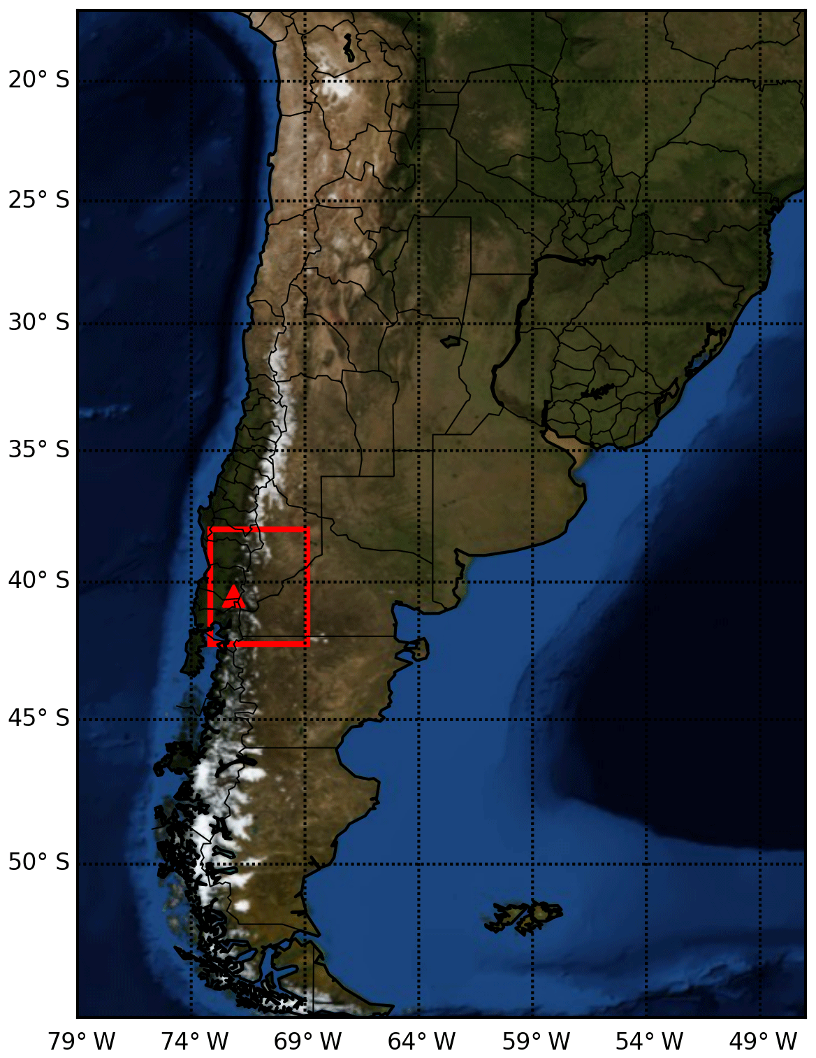
Figure 3 Domain used in the ETKF–FALL3D sensitivity tests (red square).

3.1 Ash mass loading observation simulations

The nature run and observation simulation begin at 18:00 UTC on 4 June 2011 and last for 10 d up to 00:00 UTC on 15 June, covering the domain shown in Fig. 3 with a model horizontal resolution of 0.23^∘ and a vertical resolution of 200 m. The model top is located at 20 km above the ground. The volcanic vent is located at 40.52^∘ S–72.15^∘ W at an altitude of 1420 m a.s.l.

The particle total grain size distribution (GSD) is represented by 12 classes with diameters between 2 mm (−1ϕ) and 1 µm (10ϕ) and densities ranging from 400 for the larger particles to 2100 kg m⁻³ for the smaller ones (Bonadonna et al., 2015). The vertical distribution of the source is parameterized using the Suzuki scheme considering λ=5, the settling velocity model is that of Ganser (Ganser, 1993), and the vertical and horizontal turbulent diffusion are parameterized by the similarity (Ulke, 2000) and Community Multiscale Air Quality (CMAQ) (Byun and Schere, 2006) schemes, respectively. The meteorological fields are obtained from the Global Forecasting System (GFS) analysis with a horizontal resolution of 0.5^∘, a temporal resolution of 6 h, and 27 constant pressure vertical levels.

The simulated observations represent ash mass column load (vertically integrated ash mass per unit area) estimates retrieved from satellite radiances (e.g., Prata and Prata, 2012; Francis et al., 2012; Pavolonis et al., 2013). Simulations of satellite retrievals are chosen since these observations are available almost globally and have a high spatial and temporal resolution, making them particularly appealing for the implementation of operational data assimilation systems. To represent some of the limitations of current satellite-based ash mass load retrievals, the simulated observations are available only where the true load values are between 0.2 and 10 g m⁻². The lower bound approximately corresponds to the minimum mass load that can be retrieved by state-of-the-art algorithms. Retrievals usually cannot estimate mass loads over the upper bound because the optical thickness of the corresponding ash plume is too high (e.g., Wen and Rose, 1994; Prata and Prata, 2012; Pavolonis et al., 2013). The observational error is assumed to have a random Gaussian distribution, with a standard deviation of 0.15 of the ash mass load.

For the sake of simplicity, observations are assumed to be colocated with the model grid points; we also assume that observation errors are uncorrelated (i.e., R is diagonal) and that observations are unbiased. All observations are generated assuming a clear-sky condition both above and below the ash cloud. Two nature runs were generated to evaluate the ETKF–FALL3D system: one with constant emission profiles and another with time-varying emission profiles.

3.1.1 Constant emission profile

This nature run simulation considers a source term that remains constant during the entire simulated period, with an eruption column height of 8.5 km above the vent and an A Suzuki parameter of 5.5 (Fig. 4). Figure 5a and c show the ash mass loading from the nature run and the observation simulation on 7 June at 12:00 UTC for illustrative purposes. The addition of observational error to the nature run does not significantly affect the spatial distribution or the location and intensity of the maximum concentration. The number of available observations (which depends on the thresholds described in the previous section) is time-dependent (ranging from 27 to 52 grid point observations) and, in this particular case, is primarily affected by the atmospheric circulation, which produces variations in the 3-D ash concentration within the model domain.

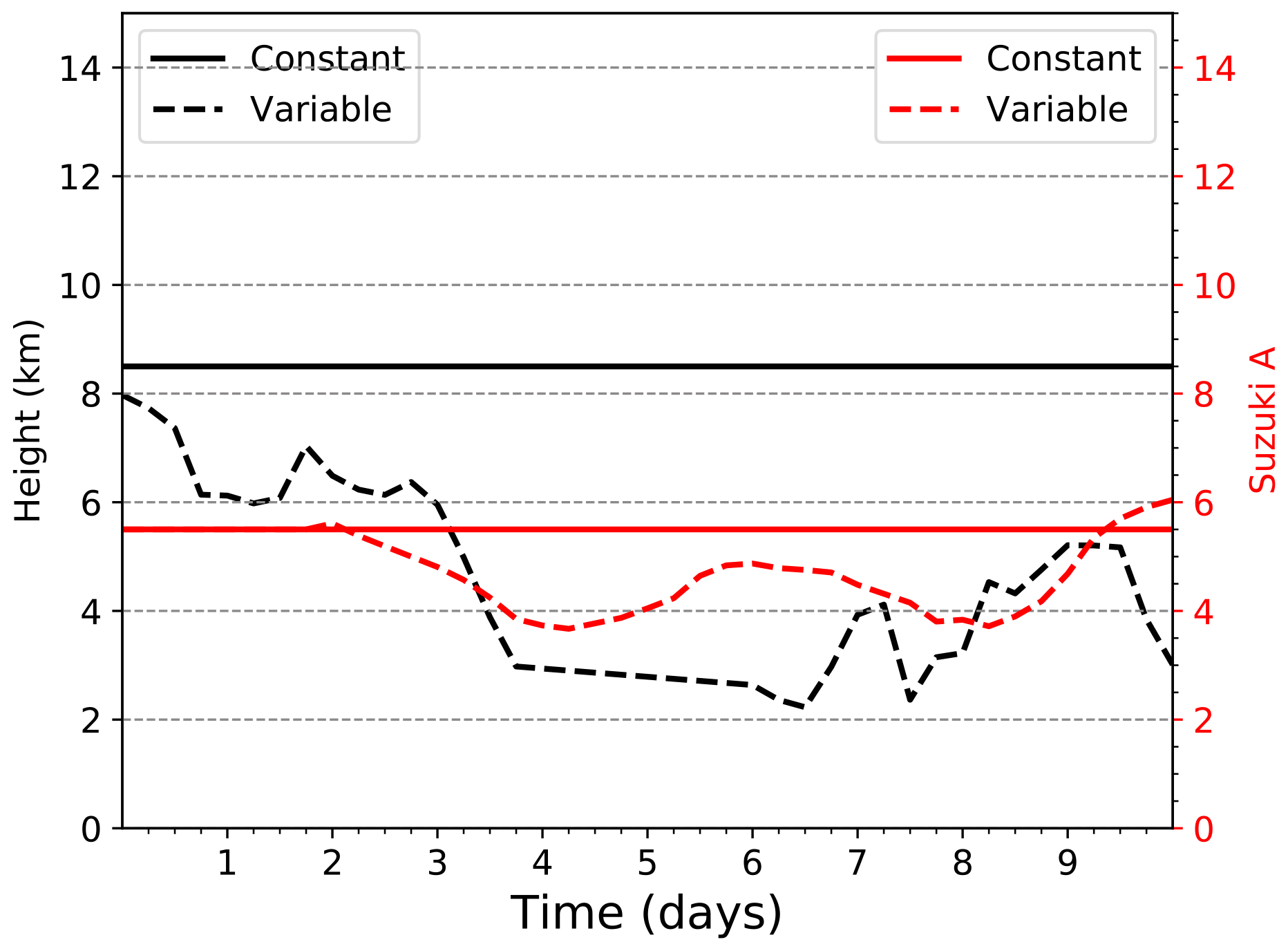
Figure 4 Nature run parameter time series for the constant (solid lines) and variable emission profiles (dashed lines) for h (black lines) and A Suzuki (red lines).

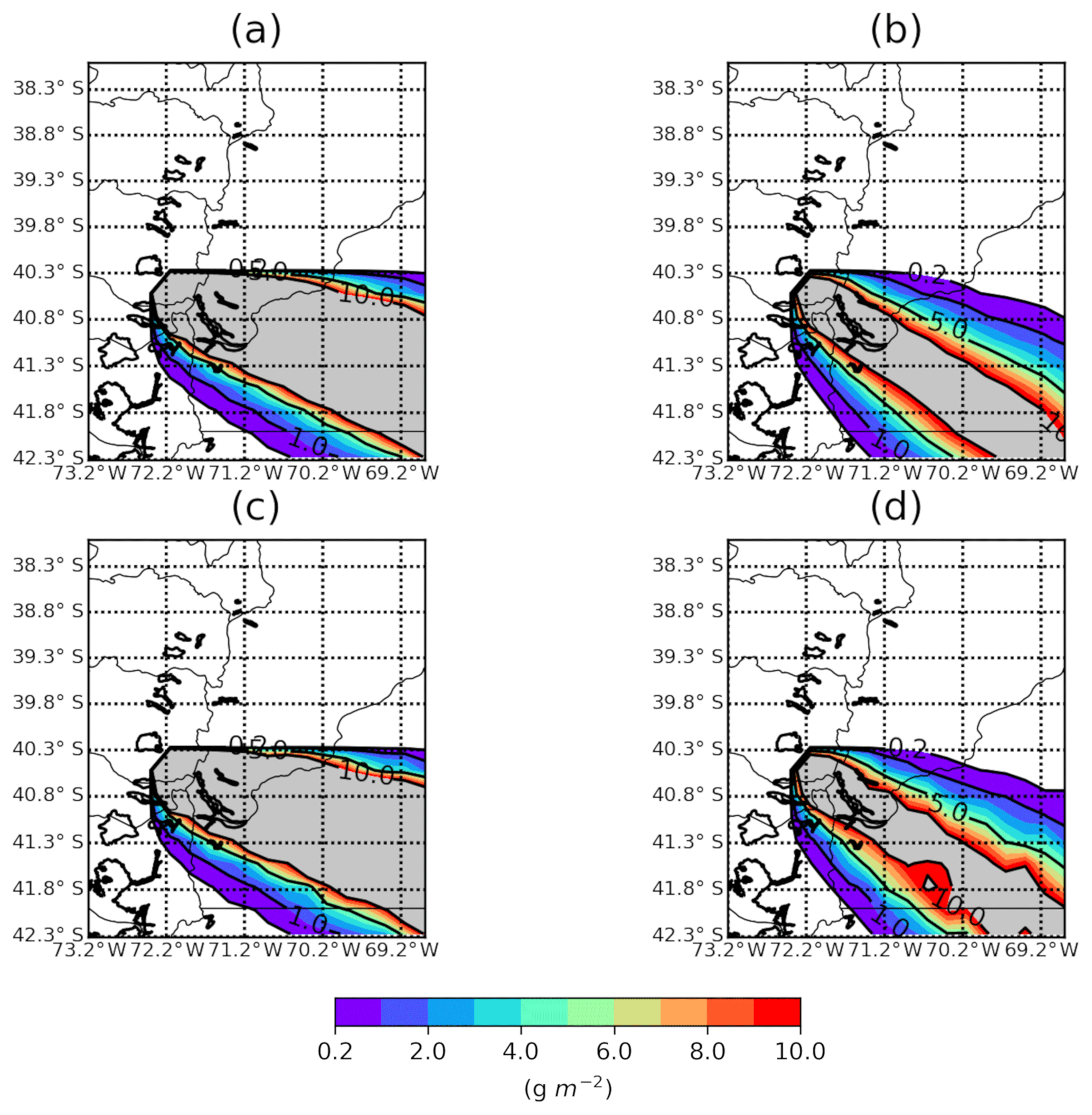
Figure 5 Ash mass loading on 7 June at 12:00 UTC for (a) the nature run with constant parameters, (c) the run with observational error and constant parameters, the (b) nature run with time-dependent parameters, and (d) the run with observational error and time-dependent parameters. Ash mass loading values outside the 0.2–10.0 g m⁻² interval are in grey.

3.1.2 Variable emission profile

In this experiment, h and A Suzuki are time-dependent (Fig. 4). In order to represent a realistic variability of the source parameters, the h evolution corresponds to the estimated heights during the 2011 Puyehue-Cordón Caulle eruption (Osores et al., 2014). Since the A Suzuki parameter cannot be directly estimated, the evolution of this parameter is simulated using an auto-regressive model (Fig. 4).

In Fig. 5b and d, the ash mass loading fields for 7 June at 12:00 UTC from the nature run and the observation simulation are shown. As has been shown for the constant parameter case, the observational error does not significantly affect the spatial distribution of the plume. In this experiment, the number of observations assimilated depends on the emission profile as well as the wind field, and it can range from 15 (on 11 June at 06:00 UTC) to 86 (on 11 June at 18:00 UTC).

3.2 Data assimilation experimental setup

In the data assimilation experiments performed in this work, the simulated observations are assimilated every 6 h. The number of ensemble members in the experiments is set to 32 (unless stated otherwise). In most experiments source parameters are assumed to be unknown and estimated within the data assimilation cycle. The model grid, boundary conditions, and all other model parameters and configuration options are set as in the nature run. The ensemble at the first assimilation cycle is initialized using zero ash concentrations for all members and a set of parameters that are sampled randomly from a Gaussian distribution whose mean and variance for each experiment are detailed below. The relaxation to prior spread (RTPS; Whitaker and Hamill, 2012) inflation approach, with a parameter of α=0.5, is applied to the state variables to reduce the impact of sampling error. For the parameters, the ensemble spread is inflated back to its original value after assimilating the observations (similar to the conditional inflation approach of Aksoy et al., 2006). This is equivalent to assuming that the parameter uncertainty is time-independent, thus preventing the parameter ensemble spread from collapsing. Covariance localization is usually required to reduce the impact of spurious correlation that results from the use of small ensemble sizes. The estimation of small correlations (e.g., between locations that are far apart from each other) is usually strongly affected by sampling noise; this is why estimated covariances are usually forced to decay with distance. Since the domain used in the data assimilation experiments is small, the impact of spurious correlations between distant grid points is less significant. For this reason, no covariance localization is used in the estimation of the state variables or the parameters. However, is important to keep in mind that if the system is extended to larger domains, using covariance localization will highly improve its performance.

Given that in the ensemble Kalman filter the distribution of ash concentration and parameters is assumed to be Gaussian, a negative ash concentration or nonphysical parameter values can result from the assimilation of observations. These nonphysical solutions must be corrected before using the analysis ensemble as initial conditions for the next ensemble forecast cycle. For ash concentration, negative values are turned into zero concentrations. In the case of eruption source parameters, nonphysical values are checked individually for each ensemble member and replaced with a random realization from a Gaussian distribution with the same mean and standard deviation as the analysis ensemble. If the randomly generated value is outside the physically meaningful range for the parameter, the process is repeated until the randomly generated value is within the physically meaningful range. The physically meaningful range for model parameters is set to 0–20 km and 0–15 for h and A Suzuki, respectively. The number of grid points and ensemble members with estimated concentrations below $-\mathrm{1.0}\times {\mathrm{10}}^{-\mathrm{4}}$ g m⁻³ is usually below 15 % of the grid points and ensemble members for which the concentration has been updated. This proportion decreased with increasing ash concentration as well as with ensemble spread. Estimated parameters for individual ensemble members fall outside the physical meaningful range less than 10 % of the times, also depending on how close to the boundaries the true parameters are and how large the parameter ensemble spread is.

One of the main hypotheses of the Kalman filter is that state variables and parameters are approximately linearly correlated with the observations. This is not true for the h parameter since in the Mastin et al. (2009) emission scheme the source strength is proportional to the fourth power of h. For this reason, instead of estimating h, we estimate h⁴ so that the estimated parameter is more linearly correlated with the observations.

In this work, several experiments are performed to study the convergence of the filter and its sensitivity to some key parameters. Two experiments are performed using the constant parameter nature run to assess filter convergence. The first experiment starts with source parameters that are higher than the true value and will be referred to as CONSTANT-UPPER; the second starts with an underestimation of the source parameters and will be referred to as CONSTANT-LOWER. The initial parameter spread for h and A Suzuki is 500 and 0.5 m, respectively, and is the same for both experiments. These experiments are compared against an experiment in which parameters remain constant at their initial value (CONSTANT-NOEST) and against an experiment in which the parameters are constant and their ensemble mean is equal to the true value (CONSTANT-TRUE).

The second set of experiments is based on the nature run with time-dependent parameters. An estimation experiment that uses the same parameter ensemble spread as in the previous experiments is performed and will be referred to as the CONTROL experiment. To evaluate the impact of performing parameter estimation in the time-dependent parameter context, an experiment in which the parameters are kept constant at the time average of the true parameters is also presented (CONTROL-NOEST).

To quantify the sensitivity of the ETKF–FALL3D system to the parameter ensemble spread, two additional experiments are performed: one in which the ensemble spread is larger than in the CONTROL experiment (HI-SPREAD), for which the spread in h and A Suzuki is 2000 and 4 m, respectively, and another experiment in which the ensemble spread is lower than in the CONTROL run (LOW-SPREAD), for which the spread in h and A Suzuki is 100 and 0.1 m, respectively. All the other configuration settings are as in the CONTROL experiment.

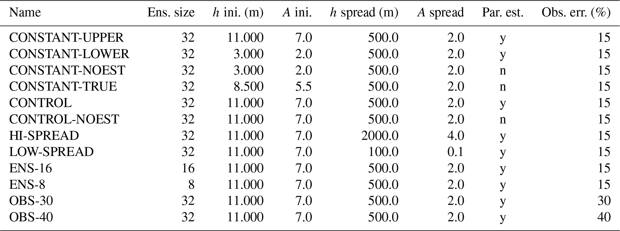
To explore the impact of modifying the ensemble size, an experiment with ensemble sizes of 8 (ENS-8) and 16 (ENS-16) is presented for which all other configuration settings are equal to the CONTROL run experiment. Finally, the impact of observation error is assessed in two experiments with observation errors that are 30 (OBS-30) and 40 % (OBS-40) of the true total mass concentration. All presented data assimilation and parameter estimation experiments are summarized in Table 2, including the statistical properties of the initial parameter ensemble. Finally, a set of simulation experiments is carried out using a larger domain to evaluate the impact of the optimized parameters upon the simulation of the ash cloud farther from the vent.

Table 2 Summary of the main parameters that distinguish the different experiments described in the text.

3.3 Performance metrics

The evaluation of the FALL3D-ETKF system is achieved by comparing the 3-D ash concentration forecast (and analysis) against the nature run and also by measuring the consistency between the estimated and the actual forecast uncertainties. The comparison is based on the RMSE, error bias, and the ensemble spread of either the forecast or the analysis, which are given by the following expressions:

$$\begin{array}{}\text{(8)}& {\displaystyle }& {\displaystyle }\text{RMSE}=\sqrt{N^{-\mathrm{1}}\sum _{i=\mathrm{1}}^N{\left({\stackrel{\mathrm{‾}}{\mathit{x}}}_{f,i}-{\mathit{x}}_{\mathit{t}\mathbf{,}\mathit{i}}\right)}^{\mathrm{2}}},\text{(9)}& {\displaystyle }& {\displaystyle }\text{BIAS}=N^{-\mathrm{1}}\sum _{i=\mathrm{1}}^N\left({\stackrel{\mathrm{‾}}{\mathit{x}}}_{f,i}-{\mathit{x}}_{\mathit{t}\mathbf{,}\mathit{i}}\right),\text{(10)}& {\displaystyle }& {\displaystyle }\text{SPREAD}=\sqrt{N^{-\mathrm{1}}\sum _{i=\mathrm{1}}^N\left(k^{-\mathrm{1}}\sum _{j=\mathrm{1}}^k{\left({\mathit{x}}_{\mathit{f}\mathbf{,}\mathit{i}}^{\mathbf{\left(}\mathit{j}\mathbf{\right)}}-{\stackrel{\mathrm{‾}}{\mathit{x}}}_{f,i}\right)}^{\mathrm{2}}\right)},\end{array}$$

where ${\stackrel{\mathrm{‾}}{\mathit{x}}}_{f,i}$ is either the forecast or analysis ensemble mean ash concentration at time and location i and ${\mathit{x}}_{f,i}^{\left(j\right)}$, and x_t,i represents their corresponding values for the jth ensemble member and the nature run, respectively. Spatial or temporal averages are obtain by summing over i.

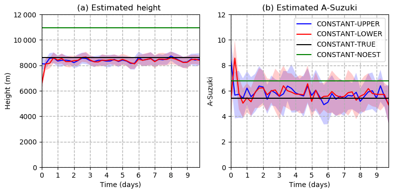
Figure 6 Optimized parameters as a function of time in the CONSTANT-UPPER (blue line), CONSTANT-LOWER (red line), CONSTANT-TRUE (black line), and CONSTANT-NOEST (green line) experiments. The shading surrounding the CONSTANT-UPPER and CONSTANT-LOWER estimated values represents ± 1 standard deviation; (a) h parameter and (b) A Suzuki parameter.

4 Results

4.1 Constant emission profile experiments

In these experiments, we explore the impact of data assimilation and parameter estimation in the steady parameter scenario. Figure 6 shows the ensemble mean and the spread of h and A Suzuki. After the first assimilation cycle, both parameters start to converge rapidly to values close to the true ones, with mean errors below 500 and 1 m, respectively. The convergence of h is faster, likely due to the strongest sensitivity of forecasted ash concentrations to column height in the surroundings of the source. The two experiments considering different initial parameter values (CONSTANT-UPPER and CONSTANT-LOWER) converge to values close to the true parameter, indicating that the parameter estimation technique is robust in finding the correct values of parameters regardless of ensemble initialization. As observed in Fig. 6, both parameter estimation experiments tend to sub-estimate the values of h and to slightly overestimate the values of A Suzuki. Figure 6 also shows the parameter ensemble spread. In these experiments, the ensemble almost always contains the true parameter value, meaning that the parameter uncertainty is well captured by the ensemble. However, it should be noted that, in these experiments, the ensemble spread of the model parameters is prescribed a priori to a value that may not be the optimal one under different conditions (e.g., if the optimal parameters are time-dependent or if other sources of uncertainty, like errors in the atmospheric circulation, are present). Sensitivity experiments to the parameter ensemble spread will be discussed in the following sections.

Figure 7a shows the time evolution of the domain-averaged RMSE for the 3-D total ash concentration forecasts. The RMSE of the parameter estimation experiments is compared against an experiment in which parameters are not estimated and are fixed at the initial value of the CONSTANT-UPPER experiment (CONSTANT-NOEST) and against an experiment in which the parameter ensemble is centered at the true value of the source parameters (CONSTANT-TRUE). Parameter estimation experiments show similar results in terms of the 6 h forecast errors, indicating the robustness of the convergence to the optimal parameter values. Moreover, both parameter estimation experiments show ash concentration errors that are similar to the one obtained in the CONSTANT-TRUE experiment and are much lower than the errors obtained in the CONSTANT-NOEST experiment, clearly showing the advantage of performing data-assimilation-based source parameter estimation. Figure 7b shows the spatially averaged ash concentration ensemble spread. One way to assess if the current parameter ensemble spread is well tuned is to compare the ash concentration forecast error and spread. If these are similar then we can assume that our uncertainty is well represented in the ensemble. In this case, the uncertainty in the ash concentration is mainly associated with the uncertainty in the source parameters. As observed, the spread values are close to the RMSE values in Fig. 7a, which indicates that after convergence of the parameters, the ensemble spread closely represents the magnitude of the errors.

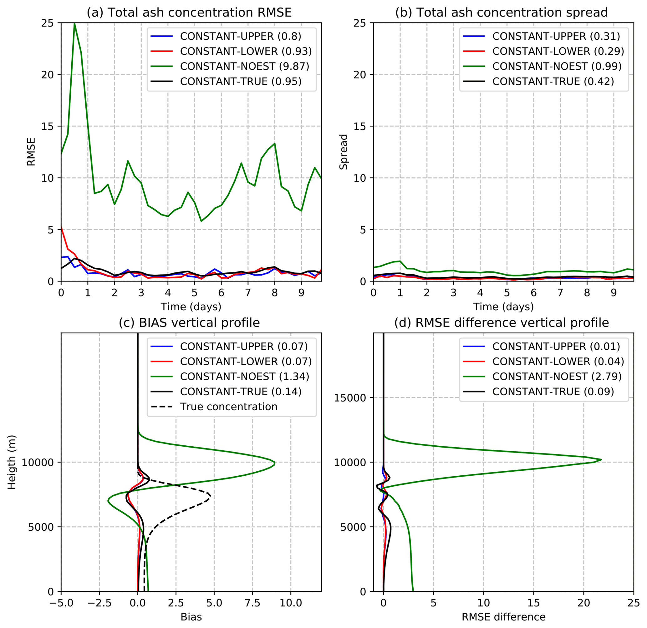
Figure 7 (a) Spatially averaged forecasted total ash concentration RMSE, (b) spatially averaged forecasted total ash concentration ensemble spread, (c) spatially averaged forecasted total ash concentration bias, and (d) the difference between the 6 h forecast and analysis total ash concentration RMSE for the CONSTANT-UPPER (blue line), CONSTANT-LOWER (red line), CONSTANT-TRUE (black line), and CONSTANT-NOEST (green line) experiments. Panels (a), (b), and (c) are computed from the 6 h ensemble forecast (all values: 10⁻³ g m⁻³).

Figure 7c shows the horizontal and time-averaged error bias for the total ash concentration as a function of height. The first 2 d have been excluded because they are considered part of the spin-up time of the filter. This figure shows that biases associated with the estimation experiments are much lower than for the CONSTANT-NOEST experiment, showing once again the advantage of optimizing the source parameters. The CONSTANT-UPPER, CONSTANT-LOWER, and CONSTANT-TRUE experiments show a small systematic underestimation of the maximum concentrations and an overestimation above and below the location of the maximum. Note that the bias is slightly lower in the parameter estimation experiments with respect to the CONSTANT-TRUE experiment.

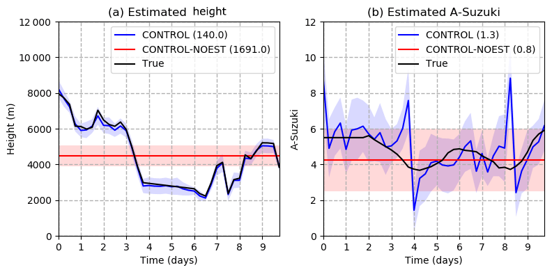
Figure 8 Optimized parameters as a function of time in the CONTROL (blue line) and CONTROL-NOEST (red line) experiments. The shading surrounding the estimated values represents ± 1 standard deviation; (a) h parameter and (b) A Suzuki parameter. The black line indicates the value of the parameters in the true run.

The fact that a biased parameter ensemble (i.e., the underestimation of h observed in Fig. 6a) produces a less biased estimation of ash concentrations (Fig. 7c) may be related to the nonlinear relationship between h and the total mass emission at the source. Since the emitted mass depends on h⁴, positive perturbations in h are associated with a much larger emission rate and are thus farther from the observations than ensemble members with negative perturbations in h. This creates a bias in the estimation of the concentrations because, even if the ensemble is centered at the true h value, positive perturbations are farther from observations than the negative ones, and therefore the ensemble mean tends to overestimate concentrations. ETKF tries to compensate for this effect by converging to a slightly biased parameter set, which reduces the error bias and the RMSE.

As observed in Fig. 7d, the analysis error in ash concentration is below the forecast error. This indicates that the ETKF method is efficient in reducing the error in the 3-D concentration field based on the information provided by a 2-D observation. This is a remarkable result in a context in which most observations are 2-D, whereas operational requirements are 3-D. This finding will be the basis for using the analysis as a better diagnostic of the state of the plume to improve the forecasts. The reason behind this lies in the structure of the forecast error covariance matrix, which is estimated from the ensemble of forecasts. This matrix contains information about the covariances between mass loading (which is the observable quantity) and the concentration at different heights from which the mass loading is obtained and which are not directly observed. In this work, reliable covariances between 3-D ash concentrations and mass loadings are obtained by taking into account the uncertainties associated with the source parameters.

4.2 Time-dependent emission experiments

These experiments use the observations simulated from the nature run with time-varying parameters (Fig. 4). The parameter ensemble is initialized with a mean h of 11 km, a mean A Suzuki of 7, and standard deviations of 0.5 and 2.0 km, respectively. Figure 8 shows the evolution in time of the optimized parameter ensemble as well as their corresponding true values, showing a good agreement. The estimation of h seems to be particularly accurate and can detect rapid variations in the eruptive column height, with RMSE values lower than 200 m throughout the experiment. For the A Suzuki parameter, the time evolution is not reproduced so accurately. There are also two sudden jumps in the estimation of A Suzuki, indicating a less well-constrained parameter value. These differences in the behavior of the estimated h and A Suzuki may be due to the higher sensitivity of the ash distribution to the eruptive column height in comparison with the A Suzuki parameter. The jumps in the estimated A Suzuki occur during periods of fast changes in h, suggesting that when h is not well estimated, A Suzuki may be modified in an attempt to compensate for errors in h.

Figure 9 As in Fig. 7 but for the experiments CONTROL (blue line) and CONTROL-NOEST (red line; all values: 10⁻³ g m⁻³).

Figure 9 shows the RMSE of the forecast for the 3-D total ash concentration. Errors in this case vary strongly with time, with larger errors corresponding to the instants in which h is larger, leading to stronger ash mass emission at the vent and consequently larger ash concentrations in the surroundings of the vent. The ensemble spread (Fig. 9b), although smaller than the error (indicating an under-dispersive ensemble), changes accordingly with more spread during the periods in which the emission is higher. These changes in the ensemble spread are a consequence of the relationship between h and mass emission at the vent. Since h deviations from the ensemble mean are almost time-independent, the associated departures in mass emission are larger during the periods of higher h, leading to a larger spread in the concentration field.

Figure 9d shows the spatially averaged reduction in the RMSE for the total ash concentration between the forecast and the analysis. The RMSE is reduced between the forecast and the analysis at almost all vertical levels, indicating that the vertical covariance structure between mass loadings and ash concentrations at different levels is well estimated, leading to accurate 3-D ash concentration estimations.

In order to assess the impact of treating the parameters as a time-dependent variable, this experiment is compared with an experiment in which data assimilation is performed but only the ash concentration field is updated. In this case, source parameters are kept constant in time at a value equal to the time average of the true parameters (CONTROL-NOEST, Fig. 8). This value is chosen to obtain a solution that is as close as possible to the one obtained with the time-dependent parameters. Figure 9 shows that the forecast RMSE and bias in the 3-D ash concentration are almost always larger in the CONTROL-NOEST experiment with respect to the CONTROL experiment. The error in the CONTROL and CONTROL-NOEST experiments becomes similar around day 3 and after day 8 because at those times instants the source parameters are close to each other (Fig. 8). Moreover, the ensemble spread for the CONTROL-NOEST experiment is almost constant in time and, because of that, changes in the forecast uncertainty are not captured (Fig. 9b). This is because time variations in the ensemble spread are mainly associated with changes in the mean values of parameters. These experiments suggest that performing data assimilation for the estimation of 3-D ash concentrations is not sufficient to properly constrain 3-D ash concentration values and that source parameters also have to be taken into account, particularly close to the source where these parameters rapidly impact concentrations.

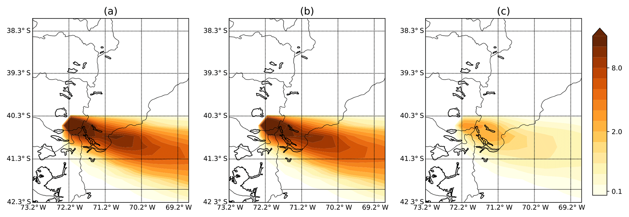
Figure 10 (a) Nature run ash concentration at flight level 200 (shaded, 10⁻³ g m⁻³); (b) as in (a) but for the 6 h forecast of ash concentration initialized from the CONTROL analysis experiment; (c) as in (b) but for the CONTROL-NOEST experiment, corresponding to the 12th assimilation cycle.

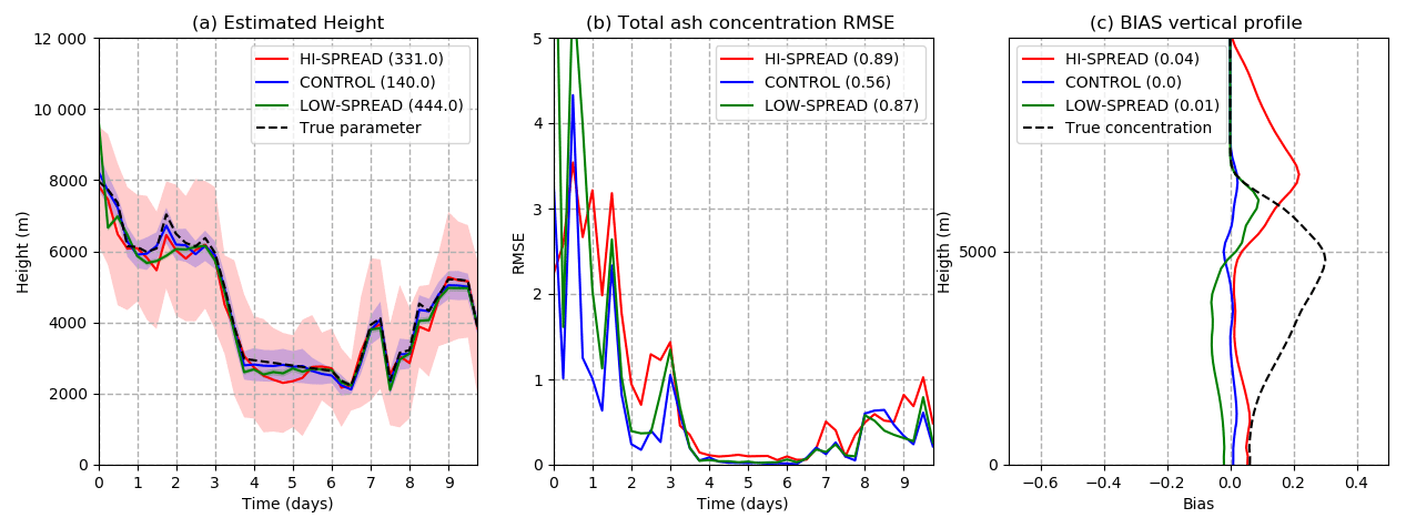
Figure 11 (a) Estimated h as a function of time for the HI-SPREAD (red line), CONTROL (blue line), and LOW-SPREAD (green line). The shading surrounding the estimated values represents ± 1 standard deviation, and the black dashed line indicates the true parameter value. (b) Spatially averaged total ash concentration 6 h forecast RMSE as a function of time (10⁻³ g m⁻³). Line color code as in (a). (c) Temporally averaged 6 h forecast bias as a function of height (10⁻³ g m⁻³). Line color code as in (a).

As an example, Fig. 10 shows the ensemble forecast mean for the CONTROL and CONTROL-NOEST experiments and the nature run at FL200 at the 12th assimilation cycle. The ash concentration pattern at this particular level is well represented by the simulation that estimates the source parameters, whereas in the CONTROL-NOEST experiment, there is a significant underestimation of the concentrations due to the underestimation of the column height at this particular time. Note that data assimilation is being performed to correct the 3-D ash concentrations in both experiments.

4.3 Sensitivity experiments

This section discusses the sensitivity of the analysis and the forecast to the parameter ensemble spread, the ensemble size, and the observation uncertainty. The purpose is to identify the potentially more important tuning parameters for the optimization of the system and how robust the system is with respect to errors in observations, which are known to exist in satellite-based ash mass loading estimations.

Figure 12 As in Fig. 11 but for the experiments CONTROL, ENS-16, and ENS-8.

To explore the sensitivity to the parameter ensemble spread, the experiments CONTROL, HI-SPREAD, and LOW-SPREAD with different parameter spreads (Table 2) are compared. Figure 11 shows the estimated h obtained in these experiments as well as the total ash concentration RMSE and bias. As observed, the CONTROL experiment gives a more accurate estimation of h and the minimum RMSE and bias. When the parameter ensemble spread is larger than in the CONTROL experiment, parameter values are systematically underestimated. As previously discussed, this can be explained by the nonlinear dependence between h and the total emitted mass. However, what is relevant from this experiment is that increasing the ensemble spread degrades the quality of the estimation and increases the impact of nonlinearities. Higher dispersion in h increases the magnitude of positive h perturbations, leading to a larger error bias, particularly above and below the maximum concentration (Fig. 11c). In the case of the LOW-SPREAD experiment, results are closer to the CONTROL experiment. However, this experiment shows a slower convergence with larger h estimation errors during the first days of the experiment. Slower convergence or a lack of convergence is expected when the parameter uncertainty is underestimated. In this case, the ETKF does not allow for large corrections in the parameter values based on the observations, basically because the error in the parameters is assumed to be small. These experiments show that the system is particularly sensitive to the parameter ensemble spread that has to be specified a priori. Moreover, in these idealized experiments, the optimal parameter ensemble spread is determined by the uncertainty in the observations and with no information regarding the changes in the true parameters in time.

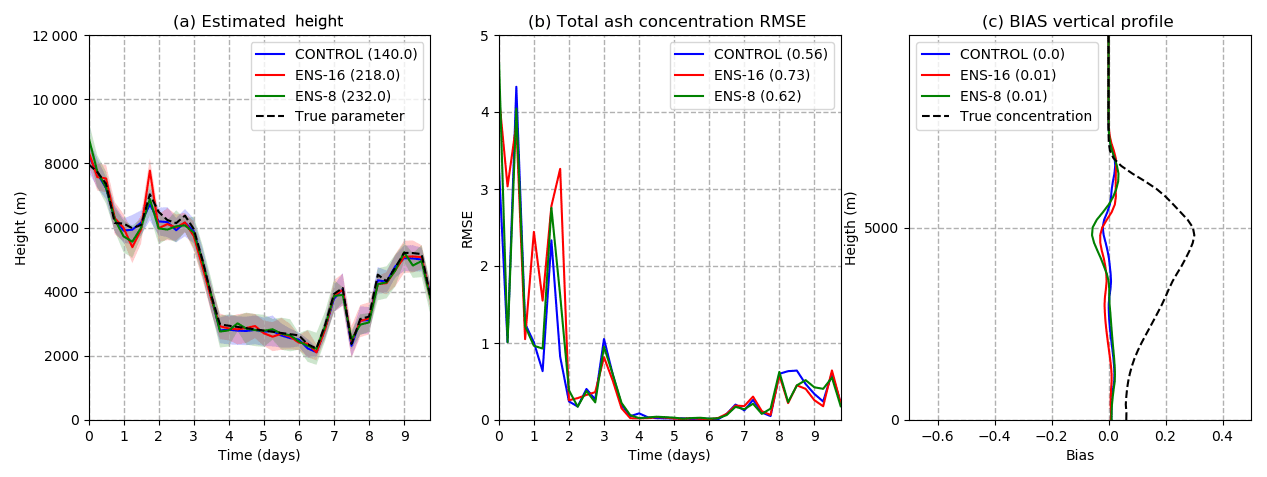
As discussed in Sect. 4.1, parameters are estimated based on their covariance with the observed quantities. In the ensemble-based data assimilation methods, these covariances are estimated directly from the ensemble, so they can be affected by sampling errors. To assess the impact of these sampling errors on the analysis, quality assimilation experiments with different ensemble sizes have been performed. Three experiments with 8, 16, and 32 ensemble members are presented (ENS-8, ENS-16, and CONTROL, respectively). Figure 12 shows the results in terms of h estimation and total ash concentration RMSE and bias. The CONTROL experiment shows a more accurate h estimation and consistently lower RMSE and bias values. However, the results are not very sensitive to the size of the ensemble. The lack of sensitivity to the ensemble size might be surprising, particularly considering that no spatial localization is being used in order to reduce the impact of sampling errors. However, note that in this case, the only source of uncertainty in the system comes from the uncertain parameters. Based on this, uncertainties have to be constrained in two dimensions. This is confirmed by the strong covariances that exist between the parameters and ash concentration within the domain (not shown). This effective low dimensionality is reinforced by the fact that the domain is small and close to the source, and, because of that, the ash concentration at most grid points is strongly correlated with the value of the uncertain source parameters.

Figure 13 As in Fig. 11 but for the experiments CONTROL, OBS-30, and OBS-40.

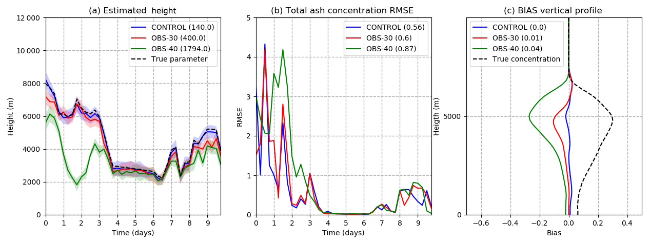
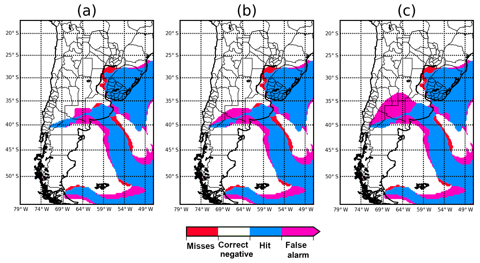
Figure 14 Ash mass loading above 0.2 g m⁻² comparison between the ensemble mean optimized parameter run, the 12 h forecast, and the 24 h forecast against the nature run over a larger domain, verifying on 8 June at 00:00 UTC (see the text for details).

The last sensitivity experiment looks into the issue of observation errors in satellite retrievals of mass loadings. In the experiments presented so far, the standard deviation of the observation errors has been assumed to be 15 % of the mass loading in the nature run. However, in real cases, uncertainties associated with mass loading estimations can be larger than that. Two additional experiments are performed to explore the impact of the magnitude of the observation errors on the estimation of source parameters and total ash concentrations with an observation standard deviation of 30 % (OBS-30) and 40 % (OBS-40) of the true mass loading value. Results from these experiments are presented in Fig. 13. As expected, the best results are obtained with the lowest observation error. However, one interesting result is that as the observation error increases, estimated h values are lower, eventually leading to substantial underestimations such as the ones seen for OBS-40 during the first days of the experiment. Moreover, this systematic underestimation of h produces an underestimation of the total ash concentrations, as is visible in the bias profiles (Fig. 13c). Under the hypothesis of the ensemble Kalman filter, an increase in the observation error leads to an increase in the RMSE of the estimation. However, in this case, the systematic component of the error is also increased. This behavior is probably a consequence of the nonlinear effects arising from the nonlinear relationship between h and the ash emission rate that has been previously discussed.

4.4 Ash concentration simulations in an extended domain simulation

The experiments discussed so far have been performed in a relatively small domain surrounding the vent. In most applications, however, it is expected that forecasts over larger domains are required. In this section, we explore the adequacy of the parameter estimation approach to generate a good estimation of ash dispersion over larger domains in an idealized context in which the atmospheric flow is perfectly known. For this purpose, a nature simulation over a larger domain is performed. This nature run is forced with the same evolution as parameters of the time-dependent parameter nature run and spanning the same period.

To see if the estimated parameters can be used to reconstruct the ash cloud far from the source, the estimated parameters are used to produce a simulation of the ash cloud over a larger domain. At each time the source parameter values in this simulation are taken from the CONTROL run parameter ensemble mean. This simulation will be referred to as CONTROL-LD. Figure 14a shows the results of comparing the ash mass loading above 0.2 g m⁻² from the experiment forced with the estimated parameters against the nature run. The comparison of these categorical variables shows that hits (i.e., grid points in which mass loadings are over the selected threshold for both the simulation and the nature run) prevail, with a lower number of false alarms and misses (i.e., grid points in which the simulation is over the threshold and the nature is not or vice versa, respectively). We note that both ash clouds are very close to each other, even far from the source, indicating that the estimated parameters are sufficient for the reconstruction of the ash plume in this ideal case.

To see if the CONTROL-LD experiment can be used to initialize short-range ash concentration forecasts over the larger domain a forecast is initialized using the CONTROL-LD ash concentrations as initial conditions and the CONTROL parameter ensemble mean as source parameters. Note that in this case, parameters remain constant during the forecast. Figure 14a and b show the 12 and 24 h forecast lead times initialized on 7 June at 12:00 and 00:00 UTC, respectively. There is a good agreement between forecasts and the nature run. For larger lead times there are more false alarms and misses as expected. This suggests that initializing a forecast from a long run forced with the optimized parameters can be a cost-effective strategy to generate short-lead-time ash concentration forecasts over a relatively large domain.

Although these results are encouraging, it should be taken into account that in more realistic situations, other sources of uncertainty (e.g., uncertainty in the flow or model errors) can significantly affect the evolution of the ash plume far from the source. In this case, the forecast quality can suffer from the estimation of the 3-D ash concentration over the entire domain based on the assimilation of mass loading observations.

5 Summary and conclusions

The estimation of time-dependent source parameters has been successful within the OSSE context. The ensemble not only produces an estimation of the covariances between the observed variables and the parameters but also provides a time-dependent estimation of the forecast uncertainty that resembles the time evolution of the forecast errors. The strong time variability of the ensemble spread is mainly associated with the relationship between column height and emitted mass.

Sensitivity experiments have been conducted to investigate how the parameter ensemble spread, the ensemble size, and the observation errors affect the results. The parameter ensemble spread produces a significant impact on the quality of the estimated concentrations and parameters. Larger ensemble spreads lead to stronger biases, both in concentrations and parameters, whereas lower ensemble spreads produce an overconfident ensemble and slower converge rates that degrade the estimation results. It is important to note that the optimal parameter ensemble spread can depend on the time variability of the estimated parameters and other sources of uncertainty like errors present in the observations and the model. The sensitivity to the ensemble size revealed that, even for this low-dimensional estimation problem, ensemble sizes up to 32 members show some improvement with respect to ensembles of 16 and 8 members, although the impact of increasing the ensemble size is smaller than the impact associated with changes in the parameter ensemble spread.

The sensitivity to the observation errors shows a particular behavior, with an increase in systematic errors both in the parameters and in the concentrations with increasing observational errors. When observation errors reach 40 % of the true ash loadings, the estimated parameters fail to converge during the first days of the experiment, leading to significantly larger errors in the ash concentration forecasts.

The experiments presented in this work are limited to a small domain surrounding the vent. Experiments on a larger domain show that the optimized parameters can be used to force an ash dispersion simulation that can reproduce the ash cloud properties far from the vent as long as the atmospheric circulation is accurately known. These simulations can be used to initialize ash dispersion forecasts over a larger domain as a computationally cheaper alternative to running a data assimilation system with covariance localization over a large domain.

The experiments discussed in this work assume a perfect model and a perfect meteorological forcing. In real-life applications, imperfections in the model and the forcing have a significant impact on the quality of ash dispersion forecasts. Previous works have shown that parameter estimation can be successfully performed in the presence of multiple sources of model error (e.g., Ruiz and Pulido, 2015). Preliminary experiments introducing errors in the meteorological forcing suggest that the current system provides a robust estimation of the source parameters in the presence of wind uncertainty. However, this aspect should be further analyzed in future studies.

Several research directions are needed from this work, including the following: (a) the improvement of the ETKF–FALL3D system through the application of covariance localization, allowing for a more efficient and accurate estimation of the ash concentrations over larger domains; (b) the inclusion of more uncertainty sources in the design of the filter, with the uncertainty in the atmospheric flow and the model formulation among the most important; (c) the assessment of the skill of the system in more realistic scenarios using real observations; (d) a better representation of the uncertainty associated with observations, considering possible covariances among observations as well as systematic biases in the observations; (e) the development of techniques that can converge to the optimal parameter ensemble spread based on the information provided by the observations (e.g., Miyoshi, 2011); and (f) the implementation of nonlinear assimilation approaches (e.g., Bocquet et al., 2010) that can better handle non-Gaussian error distributions and nonlinear relationships between the model parameters and the observable quantities.

Appendix A: ETKF formulation

A brief description of the ensemble transform Kalman filter equations are provided here. See Hunt et al. (2007) for a derivation of the equations as well as for a detailed discussion of the method. The ETKF approach solves the Kalman filter equations in the subspace defined by the ensemble perturbations (i.e., the departures of individual members from the ensemble mean). Under this framework, the update in the ensemble mean can be expressed as a linear combination of the forecast perturbations as follows:

$$\begin{array}{}\text{(A1)}& \stackrel{\mathrm{‾}}{{\mathit{s}}_t^a}=\stackrel{\mathrm{‾}}{{\mathit{s}}_t^f}+{\mathbf{S}}_t^f\stackrel{\mathrm{‾}}{{\mathit{w}}_t^a},\end{array}$$

where $\stackrel{\mathrm{‾}}{{\mathit{w}}_t^a}$ is a vector of weights of dimension k computed as

$$\begin{array}{}\text{(A2)}& \stackrel{\mathrm{‾}}{{\mathit{w}}_t^a}=\stackrel{\mathrm{̃}}{{\mathbf{P}}_t^a}({\mathbf{Y}}_t^f{)}^T{\mathbf{R}}^{-\mathrm{1}}\left(y_t-\stackrel{\mathrm{‾}}{y_t^f}\right).\end{array}$$

Here, ${\mathbf{Y}}_t^f$ is the ensemble perturbation matrix in observation space, whose ith column is computed as ${\mathbf{Y}}_t^{f\left(i\right)}=\mathcal{H}\left({\mathit{x}}_t^{f\left(i\right)}\right)-\stackrel{\mathrm{‾}}{\mathcal{H}\left({\mathit{x}}_t^f\right)}$, and $\stackrel{\mathrm{̃}}{{\mathbf{P}}_t^a}$ is the analysis covariance matrix in the subspace spanned by the ensemble members and is computed as

$$\begin{array}{}\text{(A3)}& \stackrel{\mathrm{̃}}{{\mathbf{P}}_t^a}={\left[(k-\mathrm{1})\mathbf{I}+({\mathbf{Y}}_t^f{)}^T{\mathbf{R}}^{-\mathrm{1}}{\mathbf{Y}}_t^f\right]}^{-\mathrm{1}},\end{array}$$

with I being the identity matrix of size k×k. The analysis ensemble perturbations are obtained as an optimal linear combination of the background ensemble perturbations:

$$\begin{array}{}\text{(A4)}& {\mathbf{S}}_t^a={\mathbf{S}}_t^f{\mathbf{W}}_t^a,\end{array}$$

and the weight matrix ${\mathbf{W}}_t^a$ is computed as

$$\begin{array}{}\text{(A5)}& {\mathbf{W}}_t^a={\left[(k-\mathrm{1}){\stackrel{\mathrm{̃}}{\mathbf{P}}}_t^a\right]}^{\mathrm{1}/\mathrm{2}}.\end{array}$$

Finally, the analysis ensemble is obtained as the sum of the analysis ensemble mean and the analysis perturbations:

$$\begin{array}{}\text{(A6)}& {\mathit{s}}_t^{a\left(i\right)}=\stackrel{\mathrm{‾}}{{\mathit{s}}_t^a}+{\mathbf{S}}_t^{a\left(i\right)}.\end{array}$$

Note also that, in this implementation, the tangent linear observation operator H is not applied explicitly since ${\mathbf{H}}_t{\mathbf{P}}_t^f{\mathbf{H}}_t^T$ is approximated by ${\mathbf{Y}}_t^f({\mathbf{Y}}_t^f{)}^T$. Once the analysis ensemble for the augmented state is obtained, one can proceed to the next assimilation cycle.