the Creative Commons Attribution 4.0 License.
the Creative Commons Attribution 4.0 License.
 | 27 Feb 2019
Mechanistic representation of soil nitrogen emissions in the Community Multiscale Air Quality (CMAQ) model v 5.1
Jesse O. Bash
Daniel S. Cohan
Soils are important sources of emissions of nitrogen-containing (N-containing) gases such as nitric oxide (NO), nitrous acid (HONO), nitrous oxide (N2O), and ammonia (NH3). However, most contemporary air quality models lack a mechanistic representation of the biogeochemical processes that form these gases. They typically use heavily parameterized equations to simulate emissions of NO independently from NH3 and do not quantify emissions of HONO or N2O. This study introduces a mechanistic, process-oriented representation of soil emissions of N species (NO, HONO, N2O, and NH3) that we have recently implemented in the Community Multiscale Air Quality (CMAQ) model. The mechanistic scheme accounts for biogeochemical processes for soil N transformations such as mineralization, volatilization, nitrification, and denitrification. The rates of these processes are influenced by soil parameters, meteorology, land use, and mineral N availability. We account for spatial heterogeneity in soil conditions and biome types by using a global dataset for soil carbon (C) and N across terrestrial ecosystems to estimate daily mineral N availability in nonagricultural soils, which was not accounted for in earlier parameterizations for soil NO. Our mechanistic scheme also uses daily year-specific fertilizer use estimates from the Environmental Policy Integrated Climate (EPIC v0509) agricultural model. A soil map with sub-grid biome definitions was used to represent conditions over the continental United States. CMAQ modeling for May and July 2011 shows improvement in model performance in simulated NO2 columns compared to Ozone Monitoring Instrument (OMI) satellite retrievals for regions where soils are the dominant source of NO emissions. We also assess how the new scheme affects model performance for NOx (NO+NO2), fine nitrate (NO3) particulate matter, and ozone observed by various ground-based monitoring networks. Soil NO emissions in the new mechanistic scheme tend to fall between the magnitudes of the previous parametric schemes and display much more spatial heterogeneity. The new mechanistic scheme also accounts for soil HONO, which had been ignored by parametric schemes.
- Article
(15478 KB) - Full-text XML
-
Supplement
(1073 KB) - BibTeX
- EndNote


Global food production and fertilizer use are projected to double in this half-century in order to meet the demand from growing populations (Frink et al., 1999; Tilman et al., 2001). Increasing nitrogen (N) fertilization to meet food demand has been accompanied by increasing soil N emissions across the globe, including in the United States (Davidson et al., 2012). N fertilizer consumption globally increased from 0.9 to 7.4 g N per m−2 cropland yr−1 between 1961 and 2013, with the US still among the top five N fertilizer users in the world (Lu and Tian, 2017). US N fertilizer use increased from 0.28 to 9.54 g N m−2 yr−1 during 1940 to 2015. In the past century, hotspots of N fertilizer use have shifted from the southeastern and eastern US to the Midwest and the Great Plains comprising the Corn Belt region (Cao et al., 2017). Recent studies have pointed to soils as a significant source of NOx emissions, contributing ∼20 % to the total budget globally and larger fractions over heavily fertilized agricultural regions (Jaeglé et al., 2005; Vinken et al., 2014; Wang et al., 2017).
Despite the significance of NOx emissions generated by soil microbes, policies both globally and for the continental US (CONUS) have focused largely on limiting mobile and point fossil fuel sources of NOx (Li et al., 2016). Hence, it is incumbent to strategize for the reduction of non-point soil sources of NOx emissions, especially in agricultural areas. Recent studies have shown higher soil NOx, even in nonagricultural areas like forests, to significantly impact summertime ozone in CONUS (Hickman et al., 2010; Travis et al., 2016). Consequently, it is increasingly important to estimate both N-fertilizer-induced and nonagricultural NH3 and NOx emissions in air quality models.
Soil NO emissions tend to peak in the summertime, when they can contribute 15 %–40 % of the total tropospheric NO2 column in the continental CONUS (Williams et al., 1992; Hudman et al., 2012; Rasool et al., 2016). Summer is also the peak season for ozone concentrations (Cooper et al., 2014; Strode et al., 2015) and the time when photochemistry is most sensitive to NOx (Simon et al., 2014). N oxides (NOx = NO + NO2) worsen air quality and threaten human health directly and by contributing to the formation of other pollutants. NOx drives the formation of tropospheric ozone and contributes to a significant fraction of both inorganic and organic particulate matter (PM) (Seinfeld and Pandis, 2012; Wang et al., 2013). Global emissions of NOx are responsible for one in eight premature deaths worldwide as reported by the World Health Organization (Neira, 2014). The premature deaths are a result of the link of these pollutants to cardiovascular and chronically obstructive pulmonary (COPD) diseases, asthma, cancer, birth defects, and sudden infant death syndrome. These adverse health impacts have been shown to worsen with the rising rate of reactive N emissions from soil N cycling (Kampa and Castanas, 2008; Townsend et al., 2003). NOx indirectly impacts Earth's radiative balance by modulating concentrations of OH radicals, the dominant oxidant of certain greenhouse gases such as methane (IPCC, 2013; Steinkamp and Lawrence, 2011). Nitrous acid (HONO) upon photolysis releases OH radicals along with NO, driving tropospheric ozone and secondary aerosol formation (Pusede et al., 2012). Soils and agriculture are the leading emitters of N2O, a potent greenhouse gas (IPCC, 2013).
Ammonia (NH3) also contributes to a large fraction of airborne fine particulate matter (PM2.5) (Kwok et al., 2013). Elevated levels of PM2.5 are linked to various adverse cardiovascular ailments, such as irregular heartbeat and aggravated asthma, that cause premature death (Pope et al., 2009) and contribute to visibility impairment through haze (Wang et al., 2012). NH3 gaseous emissions also influence the nucleation of new particles (Holmes, 2007). Air quality models such as the Community Multiscale Air Quality (CMAQ) model and GEOS-Chem represent bidirectional NH3 exchange between the atmosphere and soil–vegetation, analyzed under varied soil, vegetative, and environmental conditions (Cooter et al., 2012; Bash et al., 2013; Zhu et al., 2015).
NOx, NH3, HONO, and N2O are produced from both microbial and physicochemical processes in soil N cycling, predominantly nitrification and denitrification (Medinets et al., 2015; Parton et al., 2001; Pilegaard, 2013; Su et al., 2011). Nitrification is the oxidation of to whereby intermediate species such as NO and HONO are emitted along with relatively small amounts of N2O as byproducts. Denitrification is the reduction of soil ; it produces some NO, but predominantly produces N2O and N2 (Firestone and Davidson, 1989; Gödde and Conrad, 2000; Laville et al., 2011; Medinets et al., 2015). The fraction of N emitted as NO and HONO relative to N2O throughout nitrification and denitrification depends on several factors: soil temperature; water filled pore space (WFPS), which in turn depends on soil texture and soil water content; gas diffusivity; and soil pH. HONO is produced during nitrification only and is a source of NO and OH after undergoing photolysis (Butterbach-Bahl et al., 2013; Conrad, 2002; Ludwig et al., 2001; Oswald et al., 2013; Parton et al., 2001; Venterea and Rolston, 2000).
Whether N2O or N2 becomes dominant during denitrification depends on the availability of soil relative to available carbon (C), WFPS, soil gas diffusivity, and bulk density (i.e., dry weight of soil divided by its volume, indicating soil compaction and/or aeration by O2). Denitrification rates are quite low even at high soil N concentrations if available soil C is absent. However, the presence of high NO3 concentrations with sufficient available C is the inhibiting factor for the conversion of N2O to N2, keeping N2O emissions dominant during denitrification (Weier et al., 1993; Del Grosso et al., 2000). Denitrification N2O emissions are also found to increase with a decrease in soil pH in the range of 4.0 to 8.0 generally (Liu et al., 2010). Fertilizer application and wet and dry deposition add to the soil NH4 and NO3 pools, which undergo transformation to emit soil N as intermediates of nitrification and denitrification (Kesik et al., 2006; Liu et al., 2006; Redding et al., 2016; Schindlbacher et al., 2004).
Soil moisture content is the strongest determinant of nitrification and denitrification rates and the relative proportions of various N gases emitted by each. Increasing soil water content due to wetting events such as irrigation and rainfall can stimulate nitrification and denitrification. Nitrification rates peak 2–3 days after wetting, when excess water has drained away and the rate of downward water movement has decreased. Denitrification rates substantially increase and nitrification rates become much slower in wetter soils. This is also influenced by soil texture; for instance, denitrification is favored in poorly drained clay soils and nitrification is favored in freely draining sandy soils (Barton et al., 1999; Parton et al., 2001).
WFPS is a metric that incorporates the above factors. The relative proportions of NO, HONO, and N2O emitted vary with WFPS. Dry aerobic conditions (WFPS ∼0 %–55 %) are optimal for nitrification, with soil NO dominating soil N gas emissions at WFPS ∼30 %–55 % (Davidson and Verchot, 2000; Parton et al., 2001). HONO emissions have been observed up to WFPS of 40 % and dominate N gas emissions under very dry and acidic soil conditions (Maljanen et al., 2013; Mamtimin et al., 2016; Oswald et al., 2013; Su et al., 2011). Nitrification influences N2O production within the range of 30 %–70 % WFPS, whereas denitrification dominates N2O production in wetter soils. Denitrification N2O is limited by lower WFPS in spite of sufficient available and C (Butterbach-Bahl et al., 2013; Del Grosso et al., 2000; Hu et al., 2015; Medinets et al., 2015; Weier et al., 1993). As a result, NO and HONO emissions tend to decrease with increasing water content, whereas N2O emissions increase subject to available and C (Parton et al., 2001; Oswald et al., 2013).
Extended dry periods also suppress soil NO emissions by limiting substrate diffusion while water-stressed nitrifying bacteria remain dormant, allowing N substrate ( or organic N) to accumulate (Davidson, 1992; Jaeglé et al., 2004; Hudman et al., 2010; Scholes et al., 1997). Rewetting of soil by rain reactivates these microbes, enabling them to metabolize accumulated N substrate (Homyak et al., 2016). The resulting NO pulses can be 10–100 times background emission rates and typically last for 1–2 days (Yienger and Levy, 1995; Hudman et al., 2012; Leitner et al., 2017).
Higher soil temperature is critical in increasing NO emission during nitrification under dry conditions. However, N2O generated in denitrification positively correlates with soil temperature only when WFPS and N substrate availability in soil are not the limiting factors (Machefert et al., 2002; Robertson and Groffman, 2007). Recently, a nearly 38 % increase in NO emitted was observed under dry conditions (∼25 %–35 % WFPS) in California agricultural soils when soil temperatures rose from 30–35 to 35–40 ∘C (Oikawa et al., 2015). Temperature-dependent soil NOx emissions may strongly contribute to the sensitivity of ozone to rising temperatures (Romer et al., 2018). Also, some soil NO is converted to NO2 and deposited to the plant canopy, reducing the amount of NOx entering the atmosphere (Ludwig et al., 2001).
Mechanistic models of soil N emissions already exist and are used in the Earth science and soil biogeochemical modeling community (Del Grosso et al., 2000; Manzoni and Porporato, 2009; Parton et al., 2001). However, photochemical models like CMAQ have been using a mechanistic approach only for NH3, while using simpler parametric approaches for NO (Bash et al., 2013; Rasool et al., 2016). Other N oxide emissions like HONO and N2O are absent from the parametric schemes used in CMAQ (Butterbach-Bahl et al., 2013; Heil et al., 2016; Su et al., 2011). Variability in soil physicochemical properties like pH, temperature, and moisture, along with nutrient availability, strongly control the spatial and temporal trends of soil N compounds (Medinets et al., 2015; Pilegaard, 2013).
The U.S. Environmental Protection Agency (EPA) Air Pollutant Emissions Trends Data show that anthropogenic sources of NOx (excluding fertilizers) fell by 60 % in the US since 1980, heightening the relative importance of soils. Area sources of NOx like soils, along with less than expected reduction in off-road anthropogenic sources, are believed to have contributed to a slowdown in US NOx reductions from 2011–2016 (Jiang et al., 2018). Hence, accurate and consistent representation of soil N is needed to address uncertainties in their estimates.
The parameterized schemes currently implemented in CMAQ for CONUS, like Yienger–Levy (YL) and the Berkeley–Dalhousie Soil NOx Parameterization (BDSNP), consider only NO expressed as a fraction of total soil N available, without differentiating the fraction of soil N that occurs as organic N, NH4, or NO3 (Hudman et al., 2012; Rasool et al., 2016; Yienger and Levy, 1995). Moreover, these parametric schemes classify soil NO emissions as constant factors for different nonagricultural biomes or ecosystems compiled from reported literature and field estimates worldwide (Davidson and Kingerlee, 1997; Steinkamp and Lawrence, 2011; Yienger and Levy, 1995). These emission factors account for the baseline biogenic NOx emissions in addition to sources from deposition (all biomes) and fertilizer (agricultural land cover only) in the latest BDSNP parameterization (Hudman et al., 2012; Rasool et al., 2016). Despite their limitations, parameterized schemes do distinguish which biomes exhibit low NO emissions (wetlands, tundra, and temperate or boreal forests) from those producing high soil NO (grasslands, tropical savanna or woodland, and agricultural fields) (Kottek et al., 2006; Rasool et al., 2016; Steinkamp and Lawrence, 2011).
The EPA recently coupled CMAQ with the U.S. Department of Agriculture (USDA) Environmental Policy Integrated Climate (EPIC) agroecosystem model. This integrated EPIC–CMAQ framework accounts for a process-based approach for NH3 by modeling its bidirectional exchange (Nemitz et al., 2001; Cooter et al., 2010; Pleim et al., 2013). The coupled model uses EPIC to simulate fertilizer application rate, timing, and composition. Then, CMAQ estimates the spatial and temporal trends of the soil ammonium () pool by tracking the ammonium mass balance throughout processes like fertilization, volatilization, deposition, and nitrification (Bash et al., 2013). Using the EPIC-derived soil N pool better represents the seasonal dynamics of fertilizer-induced N emissions across CONUS (Cooter et al., 2012). The coupling with EPIC reduces CMAQ's error and bias in simulating total NH3 + wet deposition flux and ammonium-related aerosol concentrations (Bash et al., 2013). The BDSNP parametric scheme implemented in CMAQ also uses the daily soil N pool from EPIC (Rasool et al., 2016).
Our work builds a new mechanistic approach for modeling soil N emissions in CMAQ based on the DayCENT (Daily version of CENTURY model) biogeochemical scheme (Del Grosso et al., 2000; Parton et al., 2001), integrating nitrification and denitrification mechanistic processes that generate NO, HONO, N2O, and N2 under different soil conditions and meteorology. We compare the NO and HONO emissions estimates and associated estimates of tropospheric NO2 column, ozone, and PM2.5 with those obtained from CMAQ using the YL and BDSNP parametric schemes. For agricultural biomes, our mechanistic scheme uses daily soil N pools from the same EPIC simulations as in Rasool et al. (2016). Unlike BDSNP, which uses a total weighted soil N, the new mechanistic model tracks different forms of soil N as NH4, NO3, and organic N for different soil layers and vegetation types so that nitrification and denitrification can be represented. For nonagricultural biomes, our new mechanistic scheme uses a global soil nutrient dataset in an updated C and N mineralization framework. This enables the model to track the conversion of organic soil N to NH4 and NO3 pools on a daily scale for nonagricultural soils.
2.1 Overview of soil N schemes
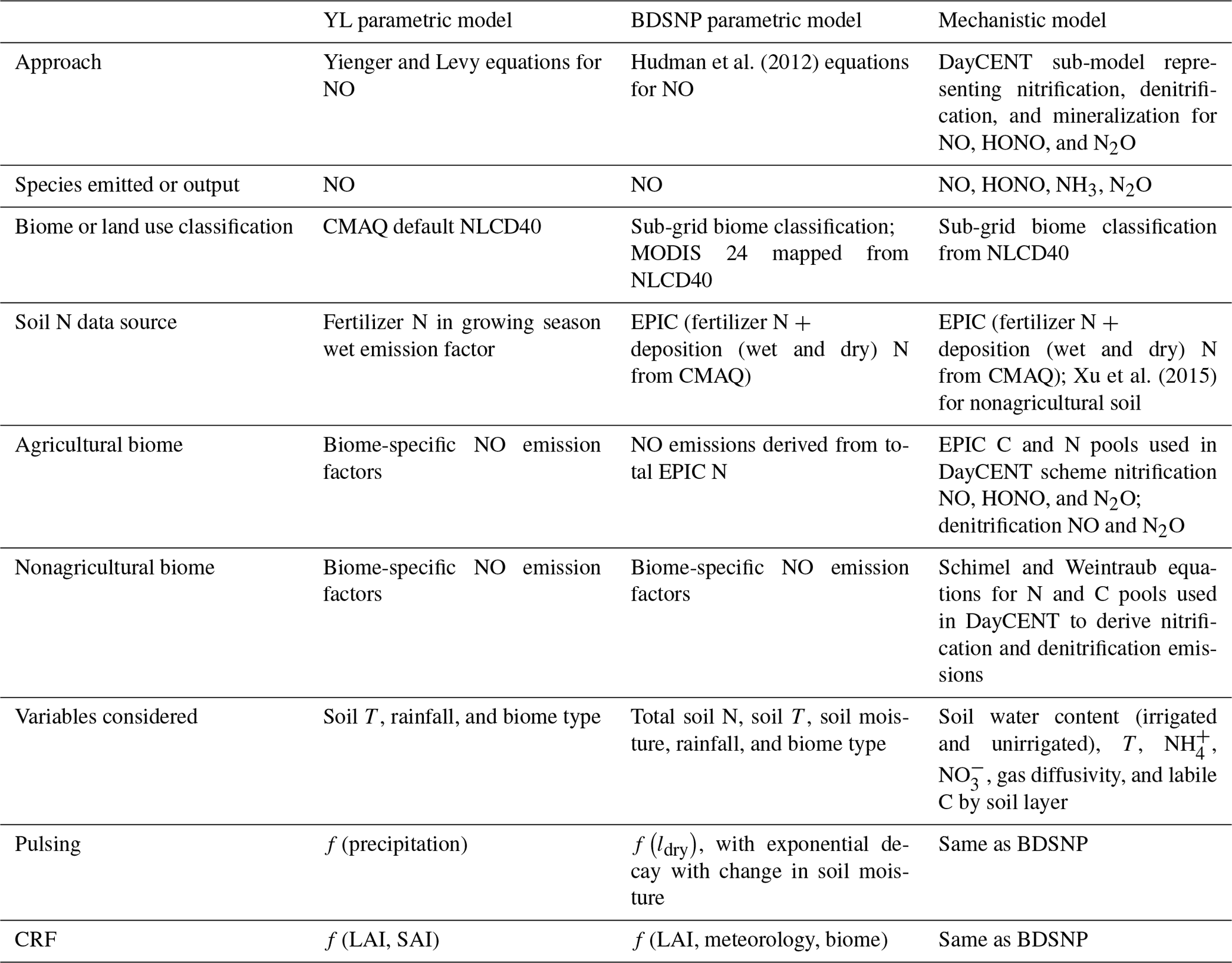
Key features of the YL and BDSNP parametric soil NO schemes and our new mechanistic scheme for soil NO, HONO, and N2O are illustrated in Fig. 1 and Table 1.
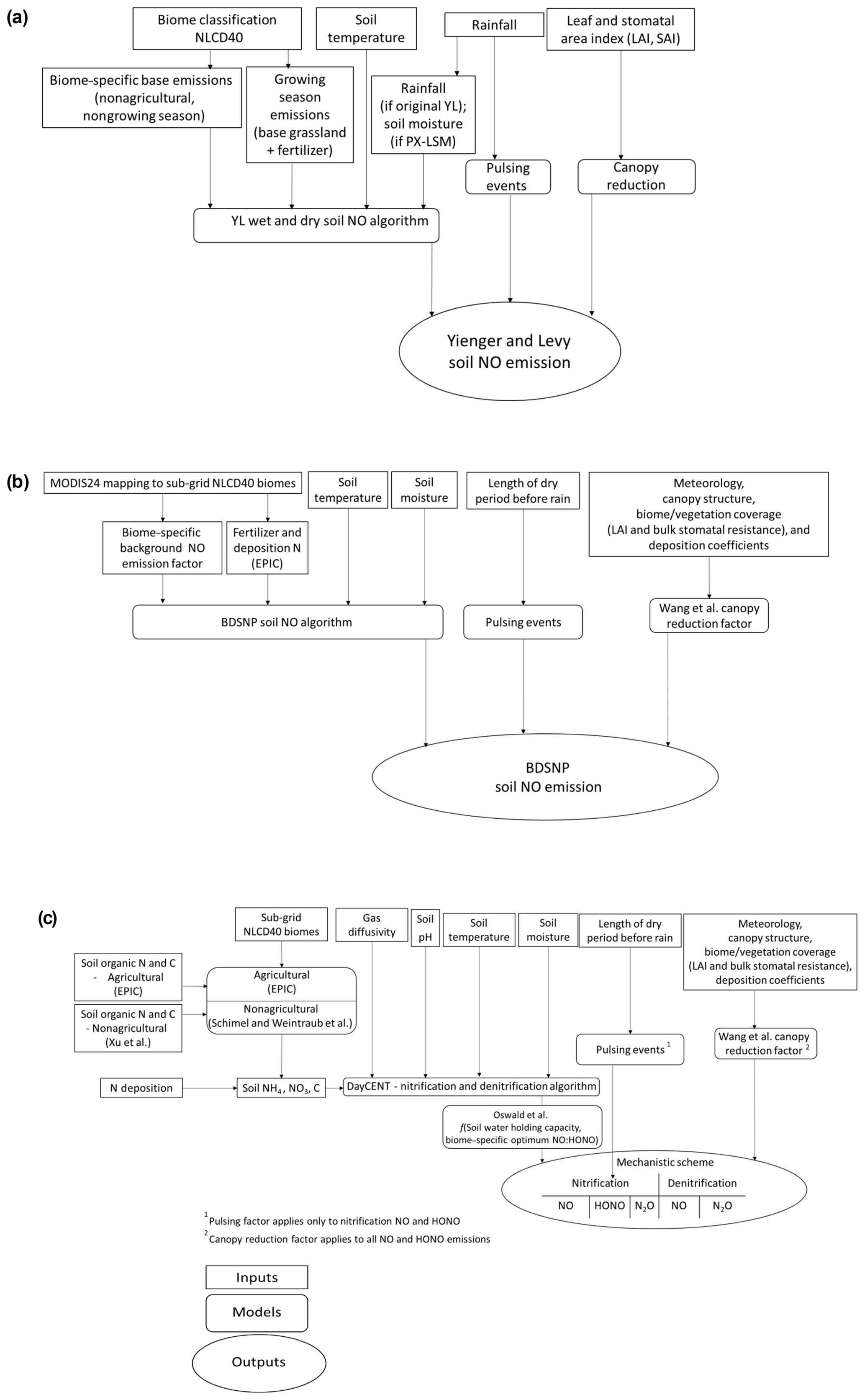
Figure 1Flowchart of the (a) Yienger and Levy (1995) (YL), (b) Berkley–Dalhousie Soil NOx Parameterization (BDSNP), and (c) mechanistic schemes for soil nitrogen (N) emissions as implemented in CMAQ.
Table 1Comparison of approaches of the parametric and mechanistic soil N emissions models.
The YL scheme, based on Yienger and Levy (1995), parameterizes soil NO emission (, in ng N m−2 s−1) in Eq. (1) as a function of biome-specific emission factors (Abiome) and soil temperature (Tsoil).
The emissions factor depends on whether the soil is wet (Abiome(w)) or dry (Abiome(d)), with the wet factor used when rainfall exceeds 1 cm in the prior 2 weeks. For dry soils, YL assumes NO emissions exhibit a small and linear response to increasing soil temperatures. For wet soils, soil NO is zero for frozen conditions, increases linearly from 0 to 10 ∘C, and increases exponentially from 10 to 30 ∘C, after which it is constant. In agricultural regions, YL assumes wet conditions throughout the growing season (May–September) and assumes 2.5 % of the fertilizer applied N is emitted as NO, in addition to a baseline NO emissions rate based on grasslands. The pulsing term (P(precipitation)) is applied if precipitation follows at least two dry weeks. The canopy reduction factor (CRF) is set as a function of leaf area index (LAI) and stomatal area index (SAI).
The Biogenic Emissions Inventory System (BEIS v3.61 used in current versions of CMAQ v5.0.2 or higher) estimates NO emissions from soils essentially using the same original YL algorithm as in Eq. (1), with slight updates accounting for soil moisture, crop canopy coverage, and fertilizer application. The YL soil NO algorithm in CMAQ distinguishes between agricultural and nonagricultural land use types (Pouliot and Pierce, 2009). Adjustments due to temperature, precipitation (pulsing), fertilizer application, and canopy uptake are limited to the growing season, assumed as 1 April to 31 October, and are restricted to agricultural areas as defined by the Biogenic Emissions Landuse Database (BELD). Unlike the original YL, the implementation of YL in CMAQ (CMAQ-YL) interpolates between wet and dry conditions based on soil moisture in the top layer (1 cm). In this study, we use the Pleim–Xiu Land Surface Model (PX-LSM) in CMAQ to compute soil temperature (Tsoil) and soil moisture (θsoil).
Agricultural soil NO emissions are based on the baseline grassland NO emission (Agrassland) plus an additional factor (fertilizer(t)) that starts at its peak value during the first month of the growing season and declines linearly to zero at the end of the growing season. The growing season is defined as April–October in CMAQ-YL, rather than being allowed to vary by latitude (original YL) or by a satellite-driven analysis of vegetation (original BDSNP). A summary of the modified YL algorithm is presented below for growing season agricultural emissions (Eq. 2).
For the nongrowing season or nonagricultural areas throughout the year, soil NO emissions are assumed to depend only on temperature and the base emissions for different biomes (Abiome) as provided in BEIS. CMAQ still uses the base emission for both agricultural and nonagricultural land types with adjustments based solely on air temperature (Tair, in K) as done in BEIS (Eq. 3). However, for the sake of simplicity we refer to “CMAQ-YL” merely as “YL”.
The original implementation of the BDSNP scheme in CMAQ v5.0.2 was described by Rasool et al. (2016). Here, we update that code for CMAQv5.1, but the formulation remains the same. Soil NO emissions, SNO, are computed in Eq. (4) as the product of biome-specific emission rates (Abiome(Navail)) and adjustment factors to represent the influence of ambient conditions. The biome-specific emission rates have background soil NO for 24 MODIS biome types from the literature (Stehfest and Bouwman, 2006; Steinkamp and Lawrence, 2011). Fertilizer and deposition emission rates based on an exponential decay after the input of fertilizer and deposition N are added to background soil NO emission rates for respective biomes. BDSNP accounts for total N from fertilizer and deposition obtained from EPIC. EPIC provides the N available from the crop-specific fertilizer soil N pool in different forms as NH4, NO3, and organic N. A final weighted total soil N pool is used by weighting the different N forms by the fraction of each crop type in each modeling grid. The soil temperature response f(Tsoil) is an exponential function of temperature (in K). Unlike YL that depends solely on rainfall, BDSNP has a Poisson function g(θ) based on soil moisture (θ) that increases smoothly first until a maximum and then decreases when soil becomes water-saturated. BDSNP also differentiates between wet and dry soil conditions and provides a more detailed representation than YL of pulsing following precipitation and of the CRF (described in Sect. 2.5).
Our new mechanistic scheme computes soil emissions of NO, HONO, and N2O by specifically representing both nitrification and denitrification. Equations (5)–(7) provide an overview of the mechanistic formulation. All functions are described in greater detail in Sect. 2.6.4. In the equations, the pulsing factor P(ldry) follows the formulation of Rasool et al. (2016). The canopy reduction factor is described in Sect. 2.5. Briefly, we note that nitrification rates (RN in Eq. 24, ) depend on the available NH4 pool, soil temperature (Tsoil), soil moisture (θsoil), gas diffusivity (Dr), and pH adjustment factors. Meanwhile, denitrification rates (RD in Eq. (25), kg N ha−1 s−1) depend on the available NO3 pool, relative availability of NO3 to C, soil temperature, gas diffusivity, and soil moisture adjustment factors.
In all our simulations, soil NH3 emission is calculated based on the bidirectional exchange scheme (Bash et al., 2013) in CMAQ.
2.2 Biome classification over CONUS
CMAQ uses the National Land Cover Database with 40 classifications (NLCD40; https://www.mrlc.gov/, last access: 22 February 2019) to represent land cover, which is used by the YL parametric scheme. However, Steinkamp and Lawrence (2011) provide soil NO emission factors ( for only 24 MODIS biomes in the BDSNP parametric scheme. Thus, the initial implementation of BDSNP in CMAQ by Rasool et al. (2016) introduced a mapping between the MODIS 24 and NLCD40 biomes to set an emission factor for each NLCD40 biome type (see Appendix Table A2). Factors were then adjusted using Köppen climate zone classifications (Kottek et al., 2006). Whereas the original implementation of BDSNP by Rasool et al. (2016) treated each grid cell based on its most prevalent biome type, our update of BDSNP for CMAQv5.1 and our mechanistic model use sub-grid biome classification, accounting for the fraction of each biome type in each cell.
The latest Biogenic Emissions Landcover Database version 4 (BELD4), generated using the BELD4 tool in the SA Raster Tools system, is used to represent land cover types consistently across both the Fertilizer Emission Scenario Tool for CMAQ (FEST-C v1.2; https://www.cmascenter.org/fest-c/, last access: 22 February 2019) and the Weather Research and Forecast (WRF) meteorological model (Skamarock et al., 2008) and CMAQ framework. BEIS v3.61 within CMAQ integrates BELD4 with other data sources generated at 1 km resolution to provide fractional crop and vegetation cover. US land use categories are based on the 2011 NLCD40 categories. FEST-C provides tree and crop percentage coverage for 194 tree classes and 42 crops (https://www.cmascenter.org/sa-tools/documentation/4.2/Raster_Users_Guide_4_2.pdf, last access: 22 February 2019). For determining fractional crop cover, the 2011 NLCD–MODIS data were used for Canada and the US in the BELD4 data generation tool of FEST-C. Tree species fractional coverage is based on 2011 Forest Inventory and Analysis (FIA) version 5.1. MODIS satellite products are used where detailed data are unavailable outside of the US.
2.3 N fertilizer
The YL scheme set fertilizer-driven soil NO emissions to be proportional to fertilizer application during a prescribed growing season: May–August for the Northern Hemisphere and November–February for the Southern Hemisphere (Yienger and Levy, 1995) or April–October for CMAQ-YL. Our implementations of both the BDSNP parameterization and mechanistic soil N schemes into CMAQ are designed to enable the use of year- and location-specific fertilizer data with daily resolution. We use FEST-C to incorporate EPIC fertilizer application data into our CMAQ runs. EPIC estimates daily fertilizer application based entirely on simulated idealized plant demand, with N stress and limitations in response to local soil and weather conditions, using linkages with WRF via FEST-C. The FEST-C interface also ensures that EPIC simulations are spatially consistent with CMAQ's CONUS domain and resolution through the Spatial Allocator (SA) Raster Tools system (http://www.cmascenter.org/sa-tools/, last access: 22 February 2019).
Because EPIC covers only the US, outside the US BDSNP uses fertilizer data regridded from Hudman et al. (2012), which scaled Potter et al. (2010) data for fertilizer N from 1994–2001 to global fertilizer levels in 2006. Our mechanistic scheme uses a more recently compiled and speciated soil N and C dataset for non-US agricultural regions, regridded from Xu et al. (2015).
2.4 N deposition
N deposition serves as a significant addition to the soil mineral N (inorganic and ) pool and hence influences soil N emissions. The YL scheme does not explicitly represent N deposition but instead sets soil emissions based on biome type. In our implementation of both the updated BDSNP and new mechanistic soil N schemes, hourly wet and dry deposition rates for both reduced and oxidized forms of N, computed within the CMAQ simulation, are added to the and soil pools.
2.5 Canopy reduction factor (CRF)
CRF is used to calculate above-canopy NO and HONO, assuming that some fraction of each is converted to NO2 and absorbed by leaves. Earlier global-scale GEOS-Chem simulations with BDSNP had a monthly averaged CRF that reduced total soil NOx by an average of 16 % (Hudman et al., 2012).
The original YL soil NO scheme (Yienger and Levy, 1995) and the in-line BEIS in CMAQ set CRF as a function of LAI and SAI. Recently, implementations of BDSNP in CMAQ and GEOS-Chem implemented CRF as a function of wind speed, turbulence, and canopy structure (Geddes et al., 2016; Rasool et al., 2016; Wang et al., 1998).
Here, we compute CRF using equations from Wang et al. (1998) for both the BDSNP and new mechanistic scheme using spatially and temporally variable land-surface parameters: surface (2 m) temperature, solar radiation (W m−2), surface pressure, snow cover, wind speed (vwind), cloud fraction, canopy structure, vegetation coverage (LAI and canopy resistances), gas diffusivity, and deposition coefficients. The final reduction factor (CRF(LAI, meteorology, biome)) for primary biogenic soil NO emissions is based on two main factors: bulk stomatal resistance (RBulk) and the land-use-specific ventilation velocity of NO (vvent,NO), calculated based on the parameters mentioned above (Eq. 8).
The ventilation velocity of NO (vvent,NO) is calculated by adjusting a normalized day- and night-specific velocity from Wang et al. (1998): 10−2 and m s−1, respectively. The adjustments are based on biome-specific LAI and canopy wind extinction coefficients (CBiome). Ctropical rainforest is the canopy wind extinction coefficient for tropical rainforests, the biome on which most canopy uptake studies for NOx are based (Eq. 9).
RBulk is a combination of various canopy resistances in series and parallel: internal stomatal resistance, cuticle resistance, and aerodynamic resistance, which have biome-specific normalized values for the MODIS 24 biomes also available in the dry deposition scheme of CMAQ. These normalized values of individual resistances are subsequently adjusted and dependent on multiple conditions for solar radiation, surface temperature, pressure, deposition coefficients, and the molecular diffusivity of NO2 in air. The calculation of RBulk based on Wang et al. (1998) has been documented and shared in the open-source BDSNP code repository (canopy_nox_mod.F) for the purpose of reproducibility (available at https://daac.ornl.gov/cgi-bin/dsviewer.pl?ds_id=_1351, last access: 22 February 2019).
2.6 Detailed description of the mechanistic soil N scheme
2.6.1 Overview
Our new mechanistic soil N model tracks the NH4, NO3, and organic C and N pools in soil separately, in contrast to the total N pool of BDSNP, and estimates NO, HONO, and N2O rather than just NO (Fig. 2). It uses DayCENT to represent both nitrification and denitrification. For agricultural biomes, we use speciated N and C pools from EPIC to drive DayCENT. For nonagricultural biomes, we use a C–N mineralization framework (Manzoni and Porporato, 2009) to estimate the inorganic N and C pools for DayCENT.
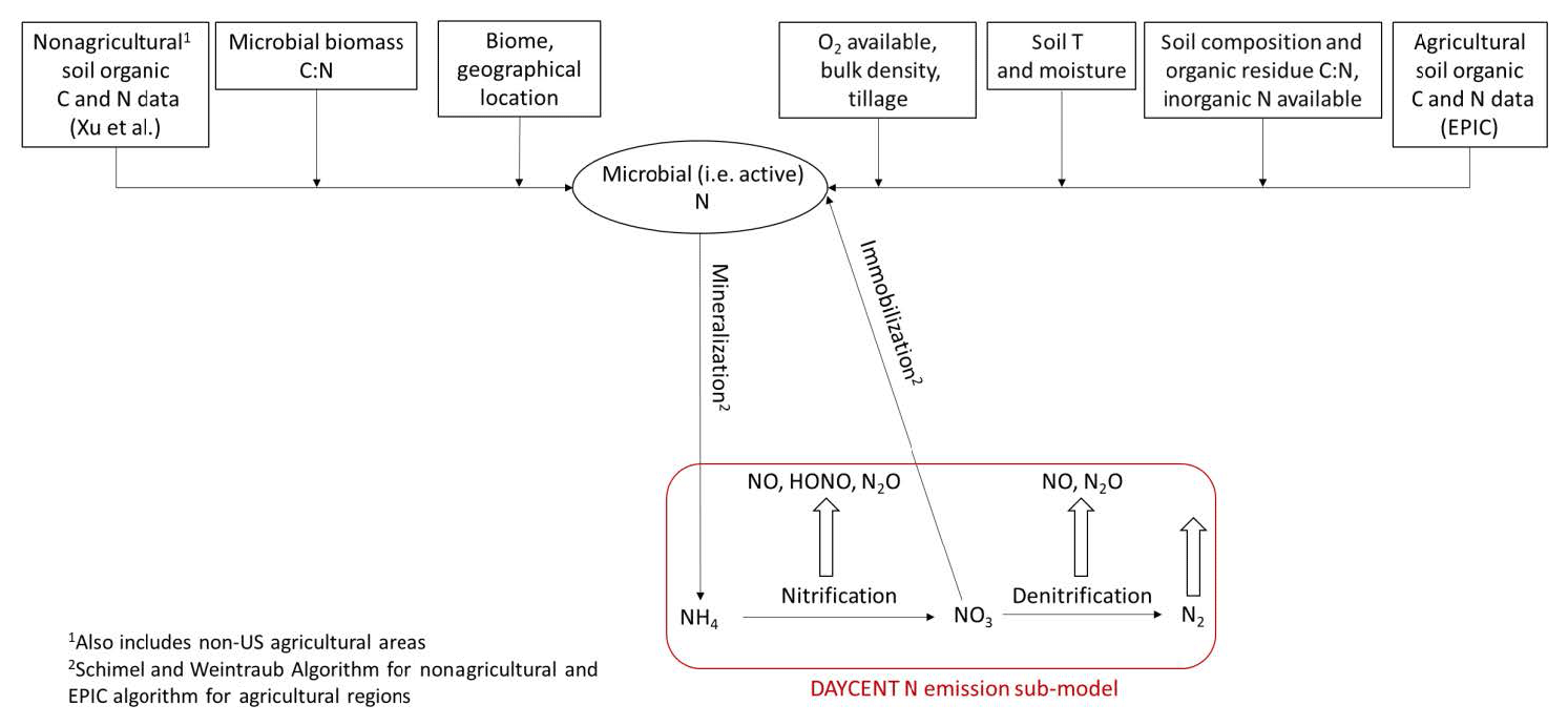
Figure 2Schematic for N transformation to estimate soil pools of ammonium (NH4) and nitrate (NO3) and the resultant nitrification and denitrification N emissions in the mechanistic model.
One of the advantages of using DayCENT is its ability to simulate all types of terrestrial ecosystems. DayCENT is one of the only biogeochemical models that not only provides a process-based representation of soil N emissions, but has also been calibrated and validated across an array of conditions for crop productivity, soil C, soil temperature and water content, N2O, and soil (Necpálová et al., 2015). Hence, mechanistic models like DayCENT yield more reliable results by applying validated controls of soil properties like soil temperature and moisture, which are the key process controls to nitrification and denitrification. More recent mechanistic models like DNDC, MicNit, ECOSYS, and COUPMODEL are quite similar to DayCENT in their representation of the nitrification and denitrification process. However, these models have not been as widely evaluated and impose greater computational costs (Butterbach-Bahl et al., 2013). DayCENT also enhances consistency in our mechanistic model by utilizing the same C–N mineralization scheme (taken from the CENTURY model; Parton et al., 2001) that is used in EPIC.
Most stand-alone applications of DayCENT and other mechanistic models have focused on the biogeochemical, climate, and agricultural impacts of soil emissions. Our linkage of DayCENT with CMAQ provides an opportunity for the first time to estimate emissions of multiple soil N species through a process-based approach and then assess their impact on atmospheric chemistry in a regional photochemical model.
2.6.2 Agricultural regions
In agricultural regions, we use EPIC to derive organic N, NH4, NO3, and C pools updated on a daily scale. EPIC follows the same approach used in the CENTURY model (Parton et al., 1994), but uses an updated crop growth model and better represents the effects of sorption on soil water content that affect leaching losses and the surface-to-subsurface flow of N. In contrast, CENTURY used monthly water leached below 30 cm of soil depth, annual precipitation, and the silt and clay content of soil (Izaurralde et al., 2006).
In EPIC, organic N residues added to the agricultural soil surface or belowground from plant or crop residues, roots, fertilizer, deposition, and manure are split into two broad compartments: microbial or active biomass and slow or passive humus. Slow or passive humus is essentially recalcitrant and nonliving in nature with very slow turnover rates ranging from centuries to even thousands of years and makes up most of the organic matter. N uptake by soil microbes from organic matter, also called “microbial biomass” or “microbial–active N”, is the living portion of the soil organic matter, excluding plant roots and soil animals larger than µm3. Although microbial biomass constitutes a small portion of organic matter (∼2 %), it is central in microbial activity: in other words, the conversion of organic N to inorganic N (Cameron et al., 2013; Manzoni and Porporato, 2009). The transformation rate of organic N to microbial N is controlled by the relative C and N content in microbial biomass, soil temperature and water content, soil silt and clay content, organic residue composition enhanced by tillage in agricultural soil, bulk density, oxygen content, and inorganic N availability. Microbial N has quicker turnover times ranging from days to weeks compared to hundreds of years for slow or passive organic matter (Izaurralde et al., 2006; Schimel and Weintraub, 2003). Hence, microbial biomass is the main clearinghouse and driver of C and N cycling in EPIC. Whether net mineralization of organic N to occurs or net immobilization of to microbial N depends strongly on the relative C and N contents in microbial biomass. Higher N content supports net mineralization, whereas higher C content supports net immobilization. C and N can also be leached or lost in gaseous forms (Izaurralde et al., 2012).
We then estimate gaseous N emissions by using the organic N, NH4, NO3, and C pools provided from EPIC/FEST-C along with relevant soil properties for agricultural biomes from the DayCENT nitrification and denitrification sub-model, as described in Sect. 2.6.4 and illustrated in Fig. 2.
2.6.3 Nonagricultural regions
We adapt the framework for linked C and N cycling from Schimel and Weintraub (2003) for nonagricultural regions, where EPIC is not applicable. This framework accounts for the mineralization of organic N by considering which element is limiting based on the relative C-to-N content in microbial biomass. If N is in excess, then the mineralization of organic N producing is favored. If C is in excess, it results in overflow metabolism that results in elevated C respiration rates not associated with microbial growth. The resultant inorganic N and C respiration rates are then applied on a temporal and spatial scale consistent with those for the EPIC agricultural pool.
To ensure mass balance, enzyme production (Eqs. 11–13) and recycling mechanisms (Eqs. 14–15) to replenish microbial biomass C are crucial. Similarly, net immobilization is assumed as was done in EPIC when we approach C-saturated conditions with time to replenish microbial N. Without such mechanisms, there is a danger to always incorrectly predict the N- or C-limited state for microbes. Also, some proportion of the microbial biomass is utilized for the maintenance of living cells (only C demand) (Eq. 14), while the rest accounts for decay and regrowth (both C and N demands) (Eqs. 16–17, 18–19) (Schimel and Weintraub, 2003; Manzoni and Porporato, 2009). Fractions of C and N in dying microbial biomass are recycled into the available microbial C and N pools. Schimel and Weintraub (2003) provide values for parameters that quantify these growth and decay processes: fraction of biome C to exoenzymes (Ke) =0.05; microbial maintenance rate (Km) =0.01 d−1; substrate use efficiency (SUE) =0.5; proportion of microbial biomass that dies per day (Kt) =0.012 d−1; proportion of microbial biomass (C or N) for microbial use (Kr) =0.85.
We represent spatial heterogeneity in soil C and N by using the Schimel and Weintraub (2003) algorithm with sub-grid land use fractions from NLCD40 to estimate the different parameters for specific nonagricultural biomes in Eqs. (10)–(20). That allows us to account for inter-biome variability in soil properties and organic and/or microbial biomass.
Mineralized N pools generated as in this framework are calculated eventually as a function of microbial biomass and the aforementioned parameters driving the net mineralization (Eqs. 18 and 21).
We map a global organic C and N pool dataset (Xu et al., 2015) onto our CONUS domain using biome-specific fractions from 12 different biome types for the conversion of these organic pools into microbial biomass pools (Xu et al., 2013). We map these 12 broader biome types to the 24 MODIS biome types with the mapping shown in Table A1. To ensure consistency with the sub-grid biome fractions for the 40 NLCD biome types (Sect. 2.2), we map the MODIS 24 biome-specific microbial ∕ organic C and N fractions to NLCD 40 (Cmicbiome and Nmicbiome; biome represents the 40 NLCD categories) with the mappings shown in Tables A2 and A3. We calculate area-weighted microbial C and N pools (SMC and SMN) using Cmicbiome and Nmicbiome that account for the inter-biome variability in the availability of soil microbial biomass. Also, spatial heterogeneity in terms of vertical stratification is crucial as emission losses from N cycling primarily happen in the top 30 cm layer. Hence, we incorporate the Xu et al. (2015) data for the top 30 cm for the organic nutrient pool and microbial C:N ratio (Cm:Nm) along with other soil properties such as soil pH, θsoil, and Tsoil. This framework (Fig. 2) enables us to estimate soil NH4, NO3, and C pools from area-weighted microbial biomass as consistently as possible with the pools that EPIC provides in agricultural regions.
2.6.4 DayCENT representation of soil N emissions
The final part of the mechanistic framework is formed by using a nitrification and denitrification N emissions sub-model adapted from DayCENT along with nitrification and denitrification rate calculations adapted from EPIC. Nitrification and denitrification rates are adapted from EPIC to maintain consistency with the NH3 bidirectional scheme in CMAQ, which uses the same. It should be noted that the coupled C–N decomposition module in the EPIC terrestrial ecosystem model is similar to that of DayCENT (Izaurralde et al., 2012, 2017; Gaillard et al., 2018). EPIC-simulated agricultural NH4 and NO3 soil pools are generated as described in Sect. 2.6.2, whereas the nonagricultural NH4 and NO3 soil pools are calculated by using the methods described in Sect. 2.6.3 (Eqs. 22–23). NH4 and NO3 soil pools drive nitrification and denitrification as shown in Eqs. (24)–(25). Variability in terms of the soil conditions influencing N emissions in nitrification and denitrification is introduced through the rates at which NH4 is nitrified (RN) and NO3 is denitrified (RD) (Eqs. 24–25).
The nitrification rate (KN) (Eq. 26) is estimated based on regulators from the soil water content, soil pH, and soil temperature (Tsoil), following the approach of Williams et al. (2008), consistent with the bidirectional NH3 scheme in CMAQ (Bash et al., 2013). The nitrification soil temperature regulator (fT) accounts for frozen soil with no evasive N fluxes (Eq. 27). The nitrification soil water content regulator (fSW) accounts for soil water content at the wilting point and field capacity (Eqs. 28–29). The regulator terms fT and fSW both get their dependent variables from land-surface outputs derived from the Meteorology–Chemistry Interface Processor (MCIP) (Otte and Pleim, 2010). However, the nitrification soil pH regulator (fpH) takes soil pH for agriculture soil from EPIC and for nonagricultural soil from a separate global dataset (Xu et al., 2015), available at both 0.01 and 1 m depths to maintain consistency with MCIP (Eq. 30). The denitrification rate (KD) (Eq. 31) is regulated by soil temperature (Eq. 34), with WFPS (Eq. 33) acting as a proxy for O2 availability and soil moisture (θsoil ) and the relative availability of NO3 and C (Eq. 32) determining N2O or N2 emissions during denitrification (Williams et al., 2008). Note that Eqs. (26) and (31) set upper limits for KN and KD, respectively.
DayCENT partitions N emissions as NOx and N2O based on relative gas diffusivity in soil compared to air (Dr) (Eq. 35). Dr is calculated based on the algorithm from Moldrup et al. (2004), which accounts for soil water content, soil air porosity, and soil type. Dr, and hence the ratio of NOx to N2O emissions () being a function of Dr, also accounts for soil texture by quantifying pore space, which is highest in coarse soil (Parton et al., 2001; Moldrup et al., 2004). DayCENT assumes 2 % of nitrified N (RN) is lost as N2O (Eq. 36). is the ratio of NOx (both NO and HONO, which photolyze rapidly to NO) to N2O, in which emissions are expressed on a g N h−1 basis. These emissions are susceptible to pulsing after rewetting of soil in arid or semiarid conditions (P(ldry)), as explained in Sect. 2.1 (Eq. 37). Denitrification NO is also calculated using the overall ratio (Eq. 38) but does not experience pulsing (Parton et al., 2001). Equation (35) does quantify as a function of Dr, but as a unitless ratio as expected.
N2O from denitrified NO3 (RD) is calculated using the partitioning function derived by Del Grosso et al. (2000) (Eq. 39). The ratio of N2 to N2O emitted as an intermediate during denitrification () is dependent on WFPS (Eq. 42) and the relative availability of NO3 substrate and C for heterotrophic respiration (Eqs. 40–41). The C available for heterotrophic respiration in the surface soil layer (labile C) (Eq. 41) is taken from EPIC for agricultural biomes and from Xu et al. (2015) for nonagricultural biomes. f(NO3:C) is controlled by variability in soil texture, accounted for by a factor k, which depends on soil diffusivity at field capacity as estimated in Del Grosso et al. (2000). Also, the NO3 pool is updated at each time step when denitrification happens (Eq. 43). Equations (40)–(42) also quantify as a unitless ratio, while still accounting for the variables influencing these ratios.
HONO is emitted as an intermediate during nitrification and has been reported in terms of a ratio relative to NO for each of 17 ecosystems by Oswald et al. (2013). In the mechanistic scheme, the proportions of HONO relative to total NOx for these 17 biomes were mapped to the closest 24 MODIS-type biome categories (Table A1) and then to the NLCD 40 types (HONOf) with the mappings in Tables A2 and A3. This allows for consistency with sub-grid land use fractions from NLCD40. HONO emissions are further adjusted to reflect their dependence on WFPS (Oswald et al., 2013). The adjustment factor fSWC reflects observations that HONO emissions rise linearly up to 10 % WFPS and then decrease until they are negligible around ∼40 % (Su et al., 2011; Oswald et al., 2013) (Eq. 45). Subsequently, total NO emission is a sum of nitrification NO emission, which is a difference of and SHONO, and denitrification NO (Eq. 46). Similarly, total N2O is a sum of (Eq. 36) and (Eq. 39). The canopy reduction factor (Sect. 2.1) is then applied to both SHONO and SNO (Eqs. 44 and 46). Finally, sub-grid-scale emission rates are aggregated for each grid cell.
2.7 Model configurations
We obtained from the U.S. EPA a base case WRFv3.7-CMAQv5.1 simulation for 2011 with the settings and CONUS modeling domain described by Appel et al. (2017), who thoroughly evaluated its performance against observations. Here, we simulate only May and July to test the sensitivity of air pollution to soil N emissions during the beginning and middle of the growing season. Each episode is preceded by a 10-day spin-up period.
Table 2 summarizes the WRF-CMAQ modeling configurations settings. The simulations use the Pleim–Xiu Land Surface Model (PX-LSM) (Pleim and Xiu, 2003) and the Asymmetric Convective Mixing v2 (ACM2) planetary boundary layer (PBL) model. The modeling domain for CMAQ v5.1 covers the entire CONUS including portions of northern Mexico and southern Canada with 12 km resolution and a Lambert conformal projection. Vertically, we use 35 vertical layers of increasing thickness extending up to 50 hPa. Boundary conditions are provided by a 2011 global GEOS-Chem simulation (Bey et al., 2001).
Table 2Modeling configuration used for the WRF-CMAQ simulations.
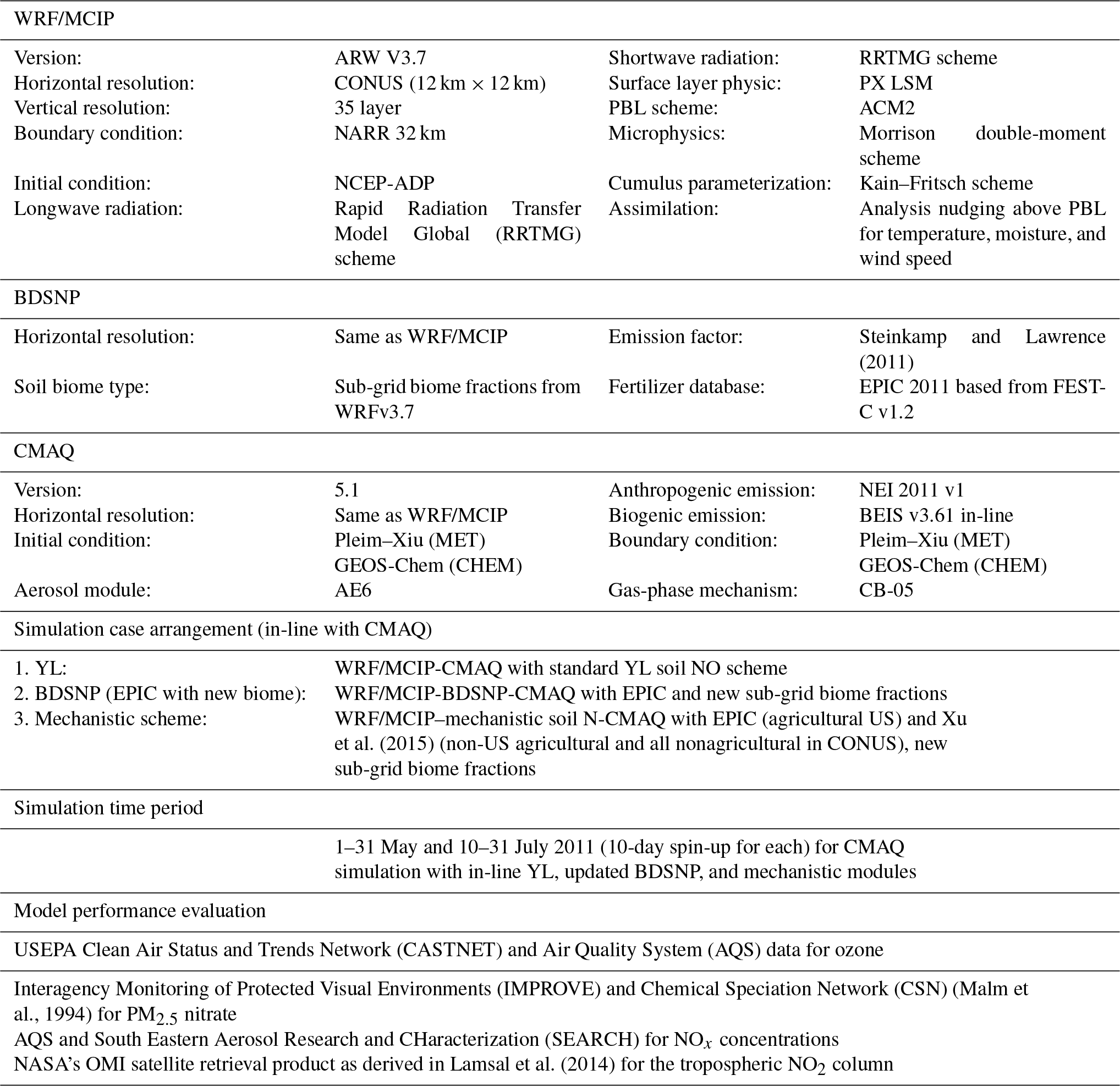
WRF simulations employed the same options as Appel et al. (2017) (summarized in Table 2). WRF outputs for meteorological conditions were converted to CMAQ inputs using MCIP version 4.2 (https://www.cmascenter.org, last access: 22 February 2019). Gridded speciated hourly model-ready emission inputs were generated using the Sparse Matrix Operator Kernel Emissions (SMOKE; https://www.cmascenter.org/smoke/, last access: 22 February 2019) version 3.5 program and the 2011 National Emissions Inventory v1. Biogenic emissions were processed in-line in CMAQ v5.1 using BEIS version 3.61 (Bash et al., 2016). All the simulations employed the bidirectional option for estimating the air–surface exchange of ammonia. We applied CMAQ with three sets of soil NO emissions: (a) standard YL soil NO scheme in BEIS; (b) updated BDSNP scheme for NO (Rasool et al., 2016) with new sub-grid biome classification; and (c) mechanistic soil N scheme for NO and HONO.
2.8 Observational data for model evaluation
To evaluate model performance for each of the three soil N cases, we employed regional and national networks: the EPA's Air Quality System (AQS; 2086 sites; https://www.epa.gov/aqs, last access: 22 February 2019) for hourly NOx and O3; the Interagency Monitoring of Protected Visual Environments (IMPROVE; 157 sites; http://vista.cira.colostate.edu/improve/, last access: 22 February 2019) and Chemical Speciation Network (CSN; 171 sites; https://www3.epa.gov/ttnamti1/speciepg.html, last access: 22 February 2019) for PM2.5 nitrate (measured every third or sixth day); the Clean Air Status and Trends Network (CASTNET; 82 sites; http://www.epa.gov/castnet/, last access: 22 February 2019) for hourly O3 and weekly aerosol PM species; and SEARCH network measurements (http://www.atmospheric-research.com/studies/SEARCH/index.html, last access: 22 February 2019) of NOx concentrations in remote areas. NO2 was also evaluated against tropospheric columns observed by the OMI aboard NASA's Aura satellite (Bucsela et al., 2013; Lamsal et al., 2014).
3.1 Spatial distribution of soil NO, HONO, and N2O emissions
Figure 3 compares the spatial distribution of soil N oxide emissions from the three schemes. The incorporation of EPIC fertilizer in BDSNP results in soil NO emission rates up to a factor of 1.5 higher than in YL, consistent with the findings of Rasool et al. (2016). Hudman et al. (2012) found nearly twice as large of a gap between BDSNP and YL in GEOS-Chem; the narrower gap here likely results from our use of sub-grid biome classification and EPIC fertilizer data (Rasool et al., 2016). The mechanistic scheme (Fig. 3c) generates emission estimates that are closer to the YL scheme but with greater spatial and temporal heterogeneity, reflecting its use of more dynamic soil N and C pools. The agricultural plains extending from Iowa to Texas with high fertilizer application rates have the highest biogenic NO and HONO emission rate, with obvious temporal variability between May and July (Fig. 3). In all of the schemes, soil N represents a substantial fraction of total NOx emissions over many rural regions, especially in the western half of the country (Fig. S1 in the Supplement). However, the aggregated budget of soil NO is much less than anthropogenic NOx from non-soil-related sources because fossil fuel use is concentrated in a limited number of urbanized and industrial locations. The percentage contribution of soil NO to total NOx aggregated across the CONUS domain varied for May–July from 15 %–20 % for YL, 20 %–33 % for updated BDSNP, and 10 %–13 % for the mechanistic scheme.
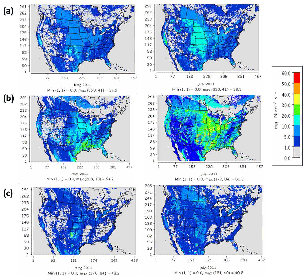
Figure 3Soil N oxide emissions on a monthly average basis for May (left) and July (right) 2011 for (a) the YL scheme (NO), (b) parameterized BDSNP scheme (NO), and (c) mechanistic scheme (NO + HONO).
Direct observations of soil emissions are sparse and most were reported decades ago. While the meteorological conditions will differ, these observations give us the best available indicator of the ranges of magnitudes of emission rates actually observed in the field. The sites encompass a variety of fertilized agricultural fields and fertilized and unfertilized grasslands (Bertram et al., 2005; Hutchinson and Brams, 1992; Parrish et al., 1987; Williams and Fehsenfeld, 1991, 1992; Martin et al., 1998). For fair comparison, the peak location or site was selected across a range of sites for a specific observation study and compared to the respective peak modeled value across sites or grids in the same spatial domain. Also, for comparison with natural unfertilized grassland observational studies based in Colorado, modeled estimates from nonagricultural grids only were selected. Overall, the YL scheme and the mechanistic scheme produce emissions estimates that are roughly consistent with the ranges of emission rates observed at each site (Table 3). By contrast, BDSNP tends to overestimate soil NO compared to these observations (Table 3).
Table 3NO emission rates (ng N m−2 s−1) observed in field studies in agricultural and grassland locations, modeled by CMAQ with the three soil N schemes for May and July 2011. Observed and modeled values are from peak location or site within a range of values across sites.

a Derived from SCIAMACHY NO2 columns. b Mechanistic scheme estimates are NO + HONO emission rates.
Table 3 also shows opposing trends for May and July soil NO estimates between YL or BDSNP and the mechanistic scheme for Iowa and South Dakota fertilized fields that make up a significant part of the Corn Belt in the US. For these regions, soil NO tends to be higher in July than in May in YL and BDSNP, but lower in July in the mechanistic scheme (Table 3). The US Corn Belt has the most synthetic N fertilizer application in April (Wade et al., 2015), which can explain the high soil NO emissions in May that decline in July. N2O emissions have been particularly observed to be highest during May–June after April N fertilizer application in the US Corn Belt, with a decline thereafter (Griffis et al., 2017). This is further confirmed in our estimates for soil N2O emissions from the mechanistic scheme, for which May estimates are higher than in July and the maximum emissions are observed in the Iowa Corn Belt (Fig. 4). However, unlike NOx emissions, for N2O no background conditions or emission inventories are in place in CMAQ's chemical transport model, so comparisons with ambient observations are not yet possible.
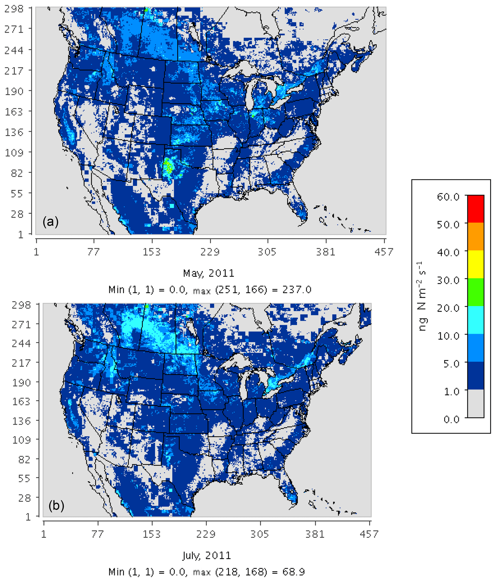
Figure 4Soil N2O emissions on a monthly average basis for May (a) and July (b) 2011 estimated from the mechanistic scheme.
3.2 Evaluation with PM2.5, ozone, and NOx observations
Model results with the three soil N schemes are compared with observational data from IMPROVE and CSN monitors for the PM2.5 NO3 component, AQS monitors for NOx and ozone, and CASTNET monitors for ozone. Both YL and the new mechanistic scheme exhibit similar ranges of bias for these pollutants (see Figs. S2, S3, S4, S5, and S6 in the Supplement). Use of the mechanistic scheme in place of YL changes soil N emissions by less than 25 ng N m−2 s−1 in most regions, corresponding to NOx concentration changes of less than 1 ppb (Fig. 5). CASTNET and IMPROVE monitors tend to be more remote than AQS and CSN monitors, many of which are located in urban regions.
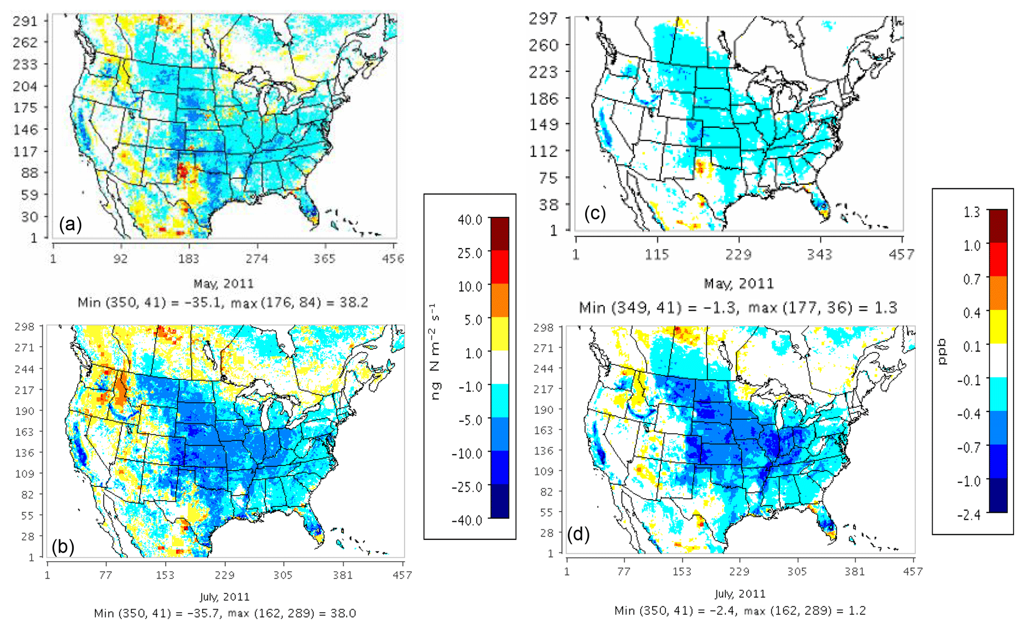
Figure 5Total NOx (NO + NO2) concentration sensitivity (right) to changes in soil NOx emissions (left) on a monthly average basis for May (a, c) and July (b, d) 2011 when switching from the YL scheme (NO) to the mechanistic scheme (NO + HONO).
At AQS monitors, switching between soil N schemes changes MB for O3 by up to ∼1.5 ppb (Fig. 6), whereas the absolute MB of models versus observations is up to ∼10 ppb (Fig. S2). For NOx, the maximum difference in MB between soil N schemes is ∼0.4 ppb (Fig. 7) compared to a maximum absolute MB of ∼10 ppb between model and observations (Fig. S3). For CASTNET monitors, the differences in MB for O3 between soil N schemes can reach a maximum of ∼1.5 ppb (Fig. 8) compared to the 6 ppb maximum absolute MB of models versus observations (Fig. S4). Similarly, for IMPROVE PM2.5 NO3, the maximum difference in MB between soil N schemes is ∼0.06 µg m3 (Fig. 9) compared to the maximum absolute MB of 0.4 µg m3 (Fig. S5). For CSN PM2.5 NO3, the maximum MB difference between soil N schemes is ∼0.1 µg m3 (Fig. 10) compared to the maximum absolute MB of ∼50 µg m3 (Fig. S6). Similar trends are observed for both May and July as illustrated in Figs. 6–10.
Overall, the mechanistic scheme tends to reduce CMAQ's positive biases for pollutants across the Midwest and eastern US, whereas BDSNP worsens overestimations in these regions for both May and July 2011 (Figs. 6–10). In addition, the negative bias in the difference means less bias compared to observations (Figs. 6–10). One reason for the differences is that the mechanistic scheme recognizes dry conditions in unirrigated fields in these regions, whereas the low WFPS threshold in BDSNP (θ=0.175 (m3 m−3)) treats most of these regions as wet and thus higher emitting.
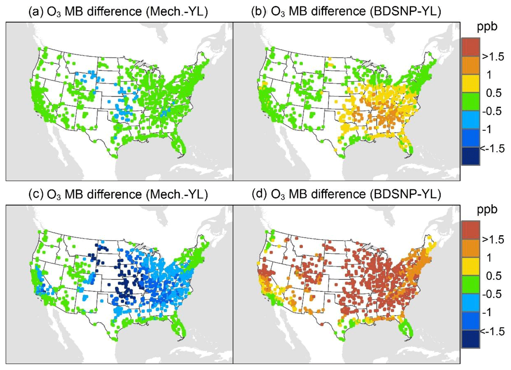
Figure 6Change in average monthly mean bias (MB) of the Community Multiscale Air Quality (CMAQ) model evaluated against the EPA Air Quality System (AQS) O3 observations for May (a, b) and July (c, d) 2011 when switching to the mechanistic (a, c) or BDSNP (b, d) scheme from YL.
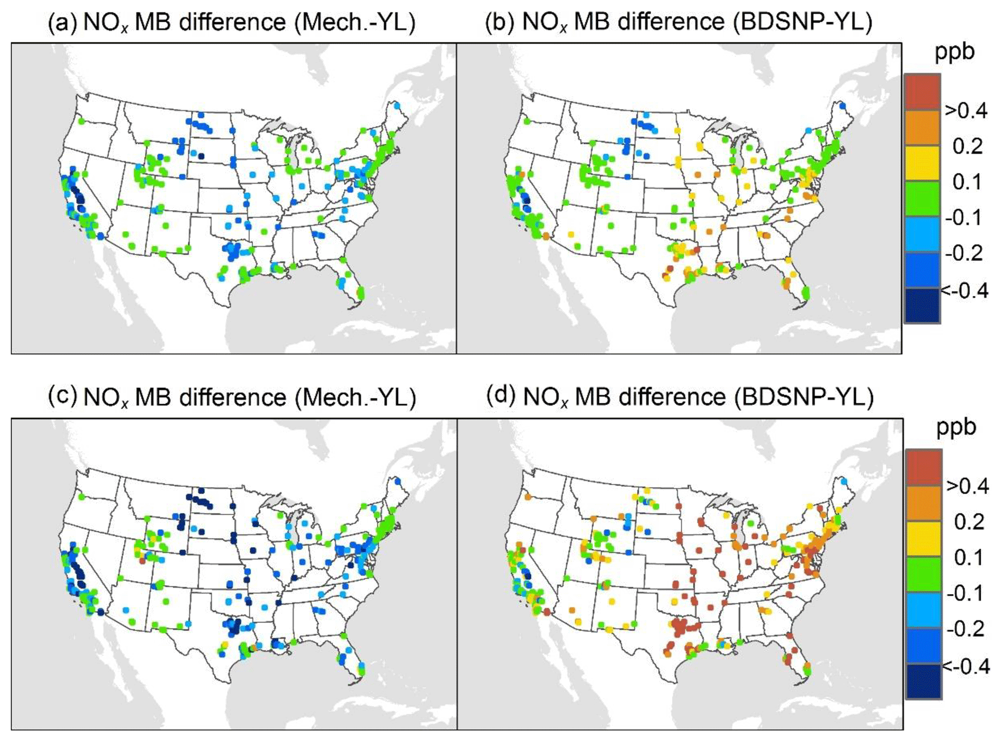
Figure 7Change in average monthly MB of CMAQ evaluated against EPA AQS NOx observations for May (a, b) and July (c, d) 2011 when switching to the mechanistic (a, c) or BDSNP (b, d) scheme from YL.
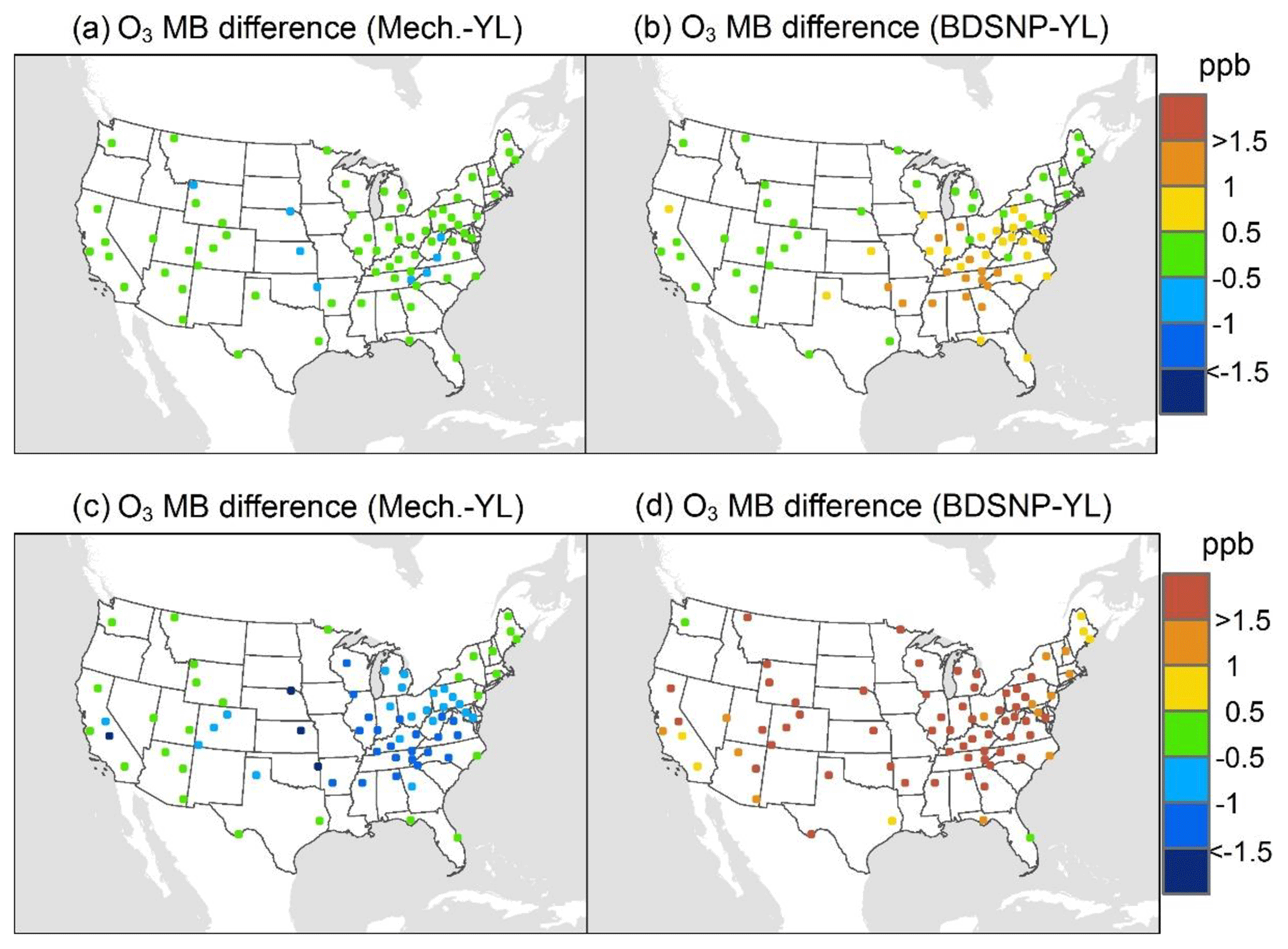
Figure 8Change in average monthly MB of CMAQ evaluated against the EPA Clean Air Status and Trends Network (CASTNET) O3 observations for May (a, b) and July (c, d) 2011 when switching to the mechanistic (a, c) or BDSNP (b, d) scheme from YL.
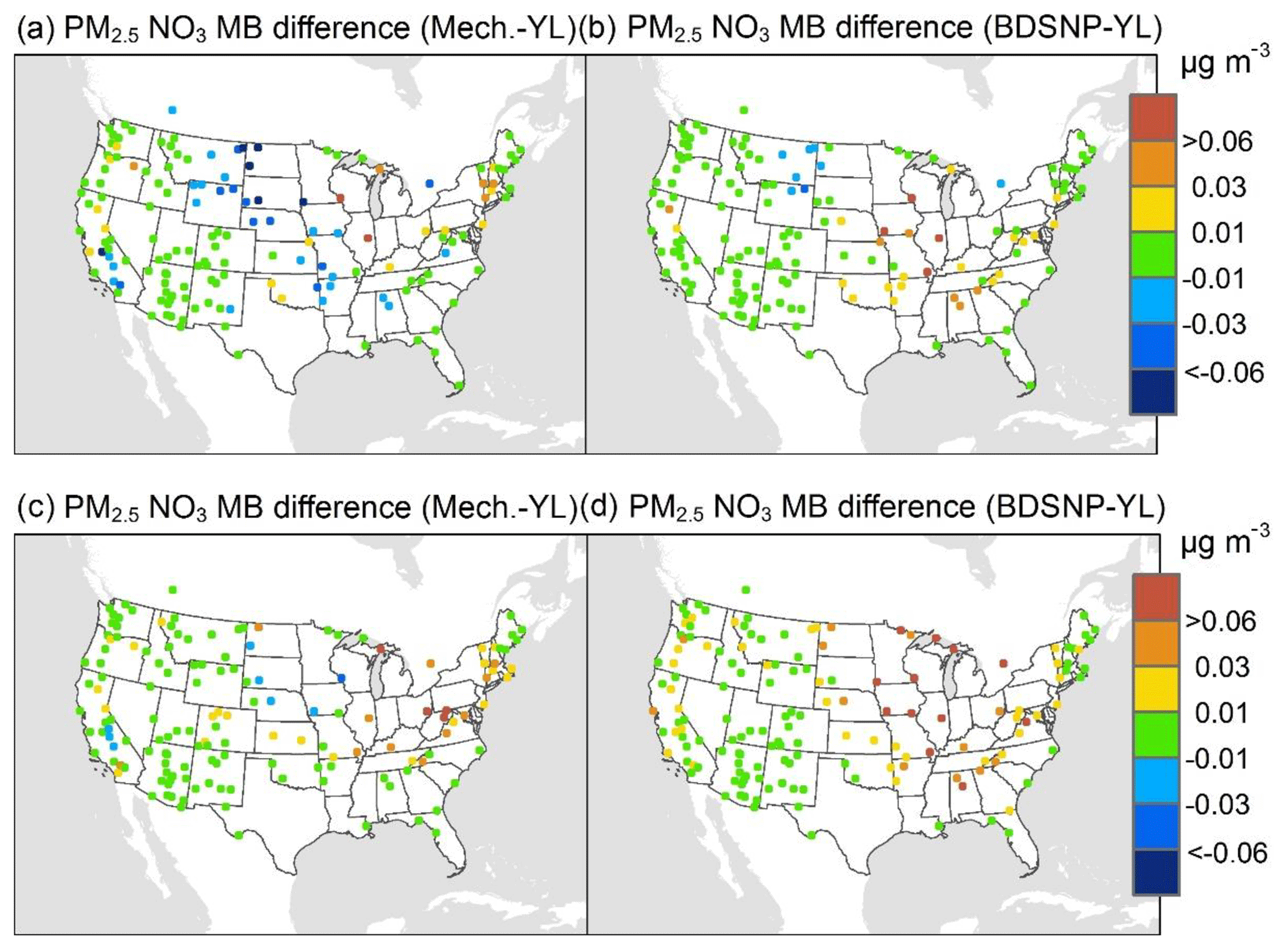
Figure 9Change in average monthly MB of CMAQ evaluated against Interagency Monitoring of Protected Visual Environments (IMPROVE) PM2.5 NO3 observations for May (a, b) and July (c, d) 2011 when switching to the mechanistic (a, c) or BDSNP (b, d) scheme from YL.
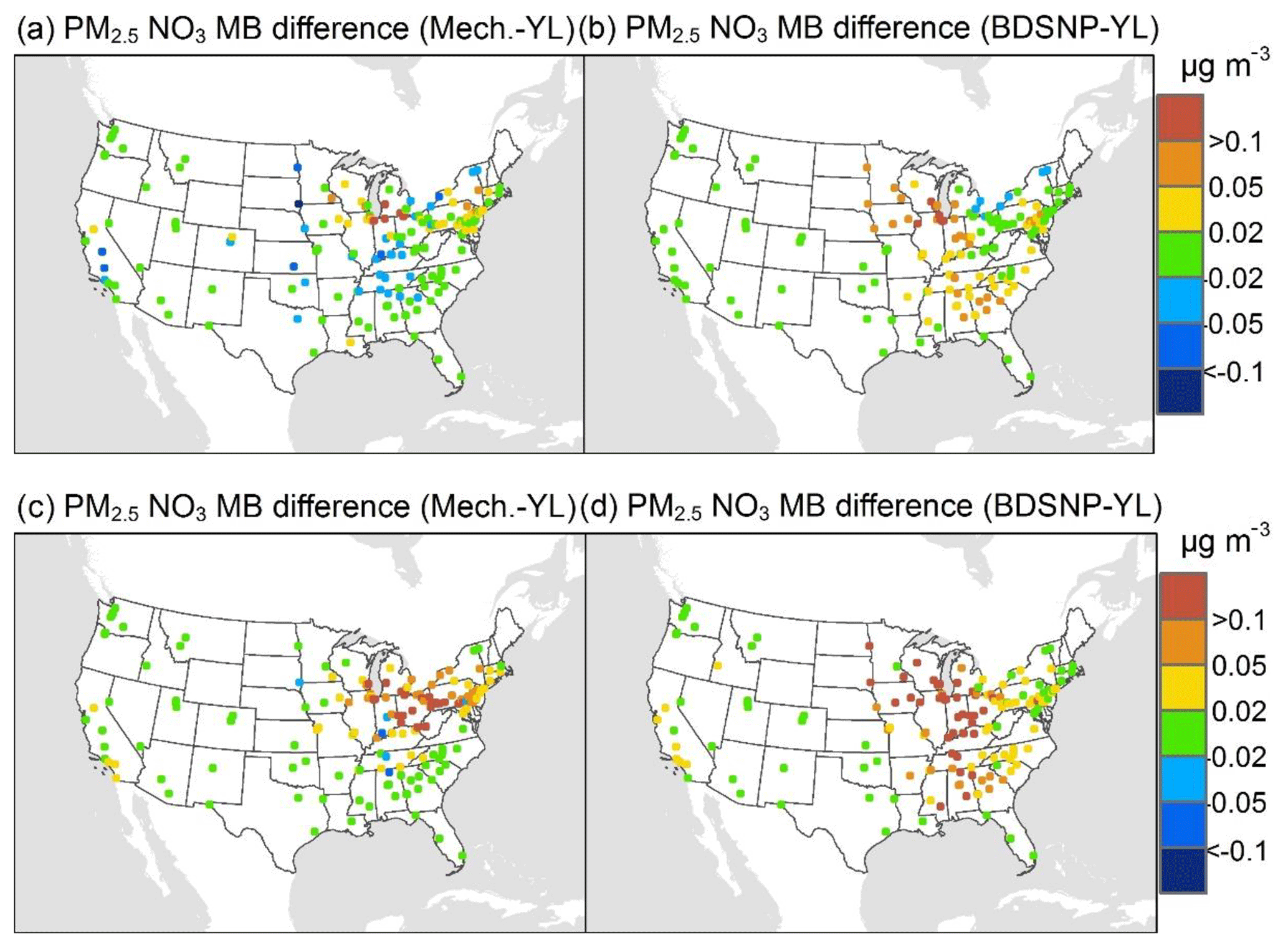
Figure 10Change in average monthly MB of CMAQ evaluated against Chemical Speciation Network (CSN) PM2.5 NO3 observations for May (a, b) and July (c, d) 2011 when switching to the mechanistic (a, c) or BDSNP (b, d) scheme from YL.
3.2.1 Evaluation with South Eastern Aerosol Research and CHaracterization (SEARCH) network NOx measurements
We analyzed how the choice of soil NO parameterization affects NOx concentrations in nonagricultural regions by using SEARCH network measurements (http://www.atmospheric-research.com/studies/SEARCH/index.html, last access: 22 February 2019). Six SEARCH sites located in the southeastern US are evaluated for May and July 2011: Gulfport, Mississippi (GFP), an urban coastal site ∼1.5 km from the shoreline; Pensacola, an outlying (aircraft) landing field (OLF) remote coastal site near the gulf ∼20 km inland; Atlanta, Georgia (Jefferson Street, JST), and North Birmingham, Alabama (BHM) – both urban inland sites; and Yorkville, Georgia (YRK), and Centreville, Alabama (CTR) – remote inland forest sites.
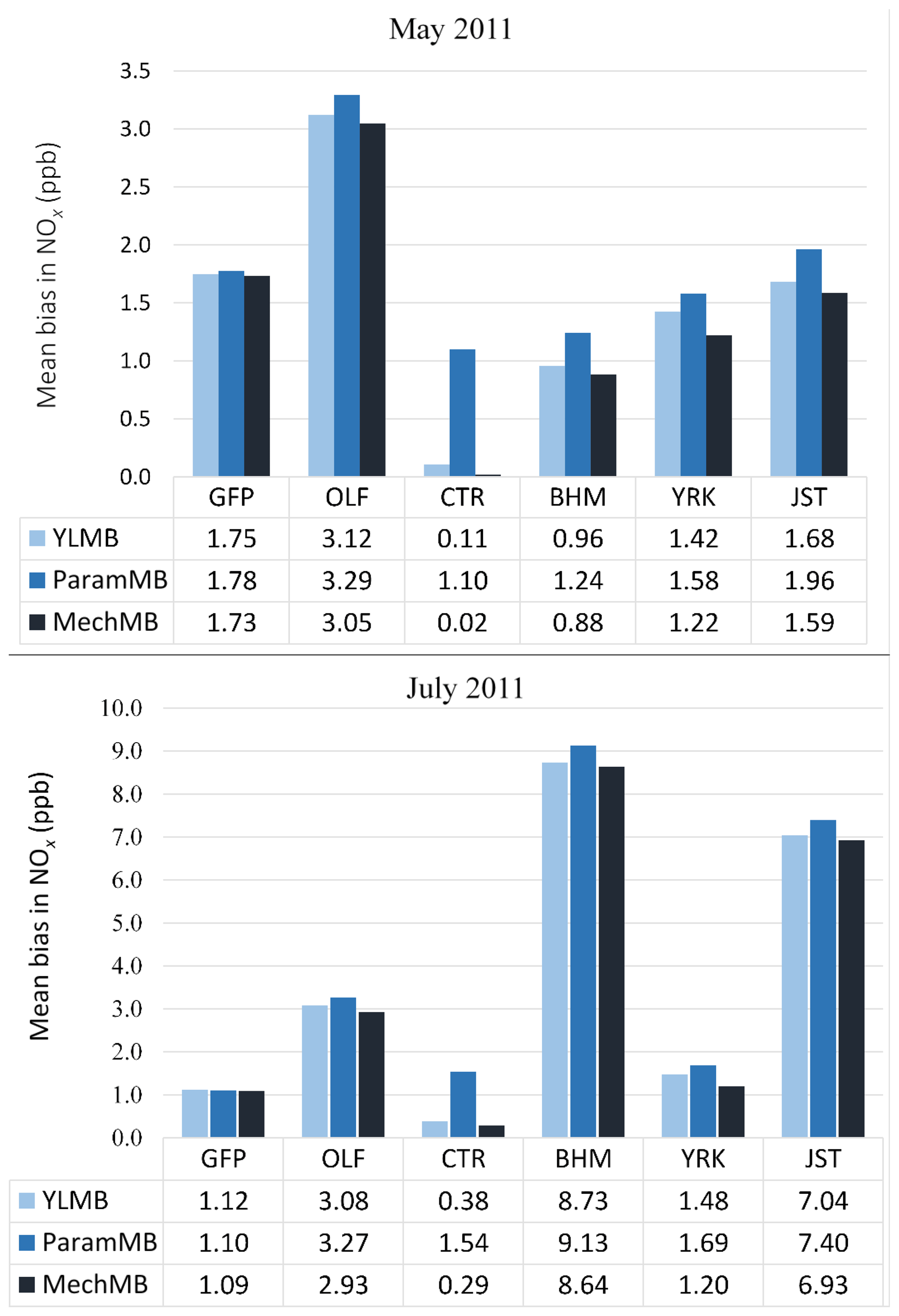
Figure 11Comparison of average monthly (May and July 2011) MB for CMAQ NOx with (a) YL, (b) BDSNP parameterized, and (c) mechanistic schemes compared to South Eastern Aerosol Research and CHaracterization (SEARCH) NOx observations in nonagricultural remote regions.
Across the southeastern US during these episodes, BDSNP estimated higher emissions than YL and the mechanistic scheme estimated lower emissions (Fig. 3). Also, CMAQ with each scheme overestimated NOx observed at each SEARCH site (Fig. 11). Thus, shifting from YL to BDSNP worsens mean bias (MB) for NOx, while the mechanistic scheme reduces MB. The impacts are most pronounced at the rural Centreville site (Fig. 11).
3.3 Evaluation with OMI satellite NO2 column observations
Tropospheric NO2 columns observed by OMI and available publicly at the NASA archive (http://disc.sci.gsfc.nasa.gov/Aura/data-holdings/OMI/omno2_v003.shtml, last access: 22 February 2019; Bucsela et al., 2013; Lamsal et al., 2014) are used to evaluate the performance of CMAQ under the three soil NOx schemes. To enable a fair comparison, the quality-assured and quality-checked (QA ∕ QC) clear-sky (cloud radiance fraction <0.5) OMI NO2 data are gridded and projected to our CONUS domain using ArcGIS 10.3.1. CMAQ NO2 column densities in molecules per cm2 are generated from CMAQ through vertical integration using the variable layer heights and air mass densities in these tropospheric layers. These NO2 column densities are then extracted for 13:00–14:00 local time across the CONUS domain to match the time of OMI overpass measurements.
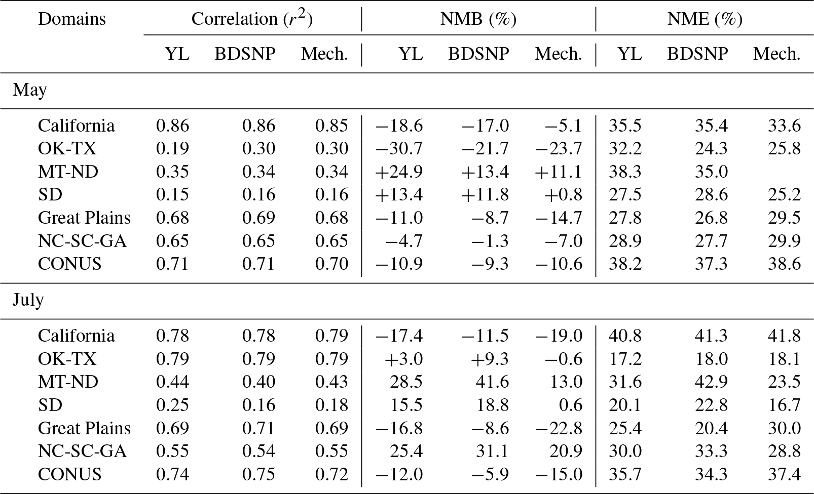
We compared CMAQ-simulated tropospheric NO2 columns with OMI data for four broad regions that showed the highest sensitivity to the soil N schemes. For May 2011, the mechanistic scheme produces higher estimates of NO2 than YL in the western US and Texas, with lower estimates in the rest of the agricultural Great Plains. In July, however, the mechanistic scheme produces lower estimates than YL in each of these regions, but the differences are narrower than in May (Fig. 12). Switching from YL to our updated mechanistic scheme improved agreement with OMI NO2 columns in the western US (for May only), Montana, North and South Dakota, North and South Carolina and Georgia (July only), and Oklahoma and Texas (red boundaries). However, switching from YL to the mechanistic scheme worsens underpredictions of column NO2 in the rest of the Midwest (black boundaries) during both May and July (Figs. 12 and 13). The mechanistic scheme improves model performance in the southeastern US and many portions of the central and western US (Table 4). Overestimation is exhibited for the eastern US across all soil N schemes and can be attributed more to the current emission inventory in CMAQ overestimating NO2 vertical column density in this region of CONUS (Kim et al., 2016). For Texas and Oklahoma, the mechanistic scheme performs better than YL but still underestimates OMI observations in May and performs well in July (Fig. 13).
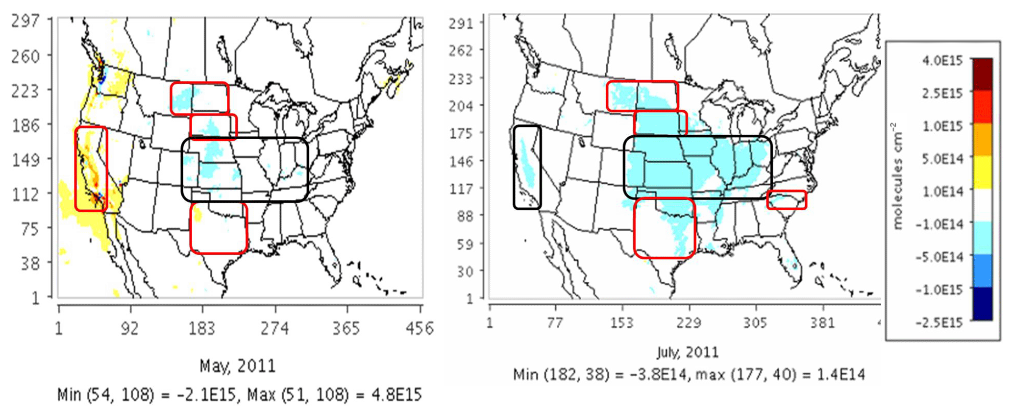
Figure 12Impact of switching from the YL scheme to the mechanistic scheme on CMAQ tropospheric NO2 column density at NASA's Ozone Monitoring Instrument (OMI) overpass time (13:00–14:00 local time) on a monthly average (May and July 2011) basis.
Table 4Statistical performance of the CMAQ modeled (with YL, updated BDSNP, and mechanistic schemes) tropospheric NO2 column for May 2011 with OMI NO2 observations for sensitive sub-domains for CONUS.
Underestimates of soil N in some regions with an abundance of animal farms, such as parts of Colorado, New Mexico, north Texas, California, the northeast US, and the Midwest, may be attributed to the lack of representation of farm-level manure N management practices, in which manure application can exceed the EPIC estimate of optimal crop demand. Farms in the vicinity of concentrated animal units often apply N in excess of the crop N requirements as part of the manure management strategy, typically increasing the N emissions (Montes et al., 2013). The USDA has reported that confined animal units or livestock production correlates with increasing amounts of farm-level excess N (Kellogg et al., 2000; Ribaudo et al., 2016). Model representations of these practices are needed to better estimate the impact of nitrogen in the environment.
Our implementation of a mechanistic scheme for soil N emissions in CMAQ provides a more physically based representation of soil N than previous parametric schemes. To our knowledge, this is the first time that soil biogeochemical processes and emissions across a full range of nitrogen compounds have been simulated in a physically realistic manner in a regional photochemical model. Our mechanistic scheme directly simulates nitrification and denitrification processes, allowing it to consistently estimate soil emissions of NO, HONO, NH3, and N2O (Figs. 1 and 2). The mechanistic scheme also updates the representation of the dependency of soil N on WFPS by utilizing parameters like water content at saturation, wilting point, and field capacity and their impact on gas diffusivity (Del Grosso et al., 2000; Parton et al., 2001).
Overall, the magnitudes of soil NOx emissions predicted by the mechanistic scheme are similar to those predicted by the YL parametric scheme and smaller than those predicted by the BDSNP scheme. In dry conditions, soil NO has been shown to be the highest compared to wet conditions with the lowest, explained by sustained high nitrification rates due to high gas diffusivity in dry conditions (Homyak and Sickman, 2014). Arid soils or dry seasons with adequate soil N due to asynchrony between soil C mineralization and nitrification have been shown to shut down plant N uptake through high gas diffusivity, causing NO emissions to increase (Evans and Burke, 2013; Homyak et al., 2016). The mechanistic scheme exhibits this spatial variability in soil NO depending on dry or wet conditions, since it accounts for their dependence on soil moisture and gas diffusivity, as well as the C and N cycling that leads to adequate soil N.
Spatial patterns of NOx emissions differ across the schemes and episodes (Fig. 3), but generally show the highest emissions in fertilized agricultural regions. During the episodes considered here, Texas experienced severe to extreme drought, while parts of the northeast and Pacific Northwest were unusually wet (http://www.cpc.ncep.noaa.gov/products/analysis_monitoring/regional_monitoring/palmer/2011/, last access: 22 February 2019). Testing for other time periods is needed to see how results differ during different seasons and as drought conditions vary. Model evaluation will also depend on the meteorological model's skill in capturing dry and wet conditions.
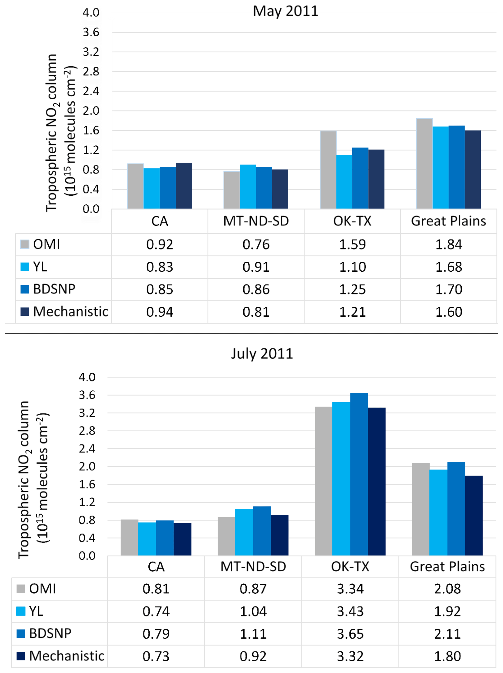
Figure 13Comparison of average monthly (May and July 2011) OMI NO2 column densities with CMAQ tropospheric NO2 column density using YL, BDSNP, and mechanistic schemes. Regions are depicted in Fig. 12.
The lower emissions of the mechanistic scheme reduce the overprediction biases for ground-based observations of ozone and PM nitrate that had been reported by Rasool et al. (2016) for the BDSNP scheme (Figs. 6–10). The mechanistic scheme reduced overpredictions of NOx concentrations at SEARCH sites in the southeastern US (Fig. 11). However, changes in performance for simulating satellite observations of NO2 columns were mixed (Figs. 12–13). The underestimation of NO2 by CMAQ with the mechanistic scheme in agricultural regions of the Midwest may be partially attributed to neglecting manure management practices from livestock operations. In the US, 60 % of nitrogen from manure produced on animal feedlot operations cannot be applied back to the same land because it is in “excess” of USDA advised agronomic rates. Most US counties with animal farms have adequate crop acres not associated with animal operations, but these are within the county, on which it is feasible to spread the excess manure at agronomic rates at certain additional cost. However, 20 % of the total US on-farm excess manure nitrogen is produced in counties with insufficient cropland for its application at agronomic rates (Gollehon et al., 2001). For areas without adequate land, alternatives to local land application such as energy production (for example, biofuel) are needed. In the absence of such a mitigation strategy, excess manure N applied on soil contributes to reactive N emissions and leaching (Ribaudo et al., 2003, 2012).
Although this work represents the most process-based representation of soil N ever introduced to a regional photochemical model, limitations remain. EPIC still lacks a complete representation of farming management practices like excess N applied as part of a nutrient management strategy for livestock, which can increase soil N pools and associated emissions. Developing and evaluating these models to address management decisions is challenging as they are often regionally specific and based on expert knowledge including regional and global economics and biogeochemical processes that have yet to be codified into a predictive system. Some aspects of soil N biogeochemistry remain insufficiently understood, especially as they relate to HONO emissions. Nevertheless, the mechanistic approach introduced here will make it possible to incorporate future advancements in understanding C and N cycling processes.
For future work, there is a need for more accurate representation of actual farming practices beyond the generalizations made by the EPIC model. Model development should be continued to better constrain N sources such as rock weathering, which are still ignored for estimating soil N emissions. Recently, Houlton et al. (2018) postulated that bedrock weathering can contribute an additional 6 %–17 % to global inorganic soil N for different natural biomes. There is also a need for more field observations of soil N emissions to better evaluate the spatial and temporal patterns simulated by the models.
The modified and new source code, inputs, and sample outputs along with the user manual giving details on implementing the new mechanistic module in-line with CMAQ version 5.1, as used in this work, are available on the Oak Ridge National Laboratory Distributed Active Archive Center for Bio-geochemical Dynamics (Rasool et al., 2018; https://doi.org/10.3334/ORNLDAAC/1661). Source codes for CMAQ version 5.1 and FEST-C version 1.2 are both open source and available with applicable free registration at http://www.cmascenter.org (last access: 22 February 2019). The Advanced Research WRF model (ARW) version 3.7 used in this study is also available as a free open-source resource at http://www2.mmm.ucar.edu/wrf/users/download/get_source.html (last access: 22 February 2019).
Table A1List of 24 MODIS soil-biome-based Cmic, Nmic, and HONOf emission factors (%) derived from Xu et al. (2013) and Oswald et al. (2013).
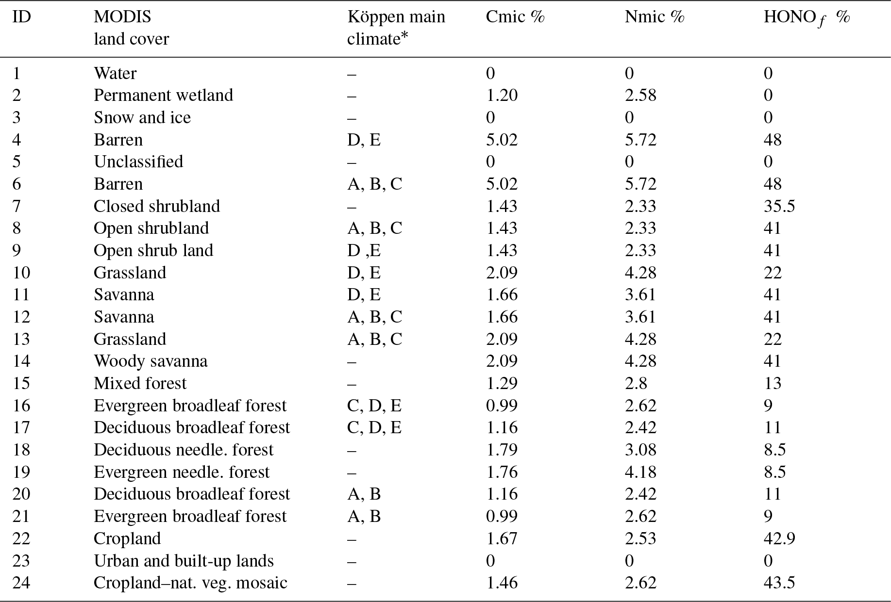
* A – equatorial, B – arid, C – warm temperature, D – snow, E – polar
Table A2Mapping table to create the MODIS 24 soil biome map based on NLCD40 MODIS land cover categories for updated BDSNP parameterization.
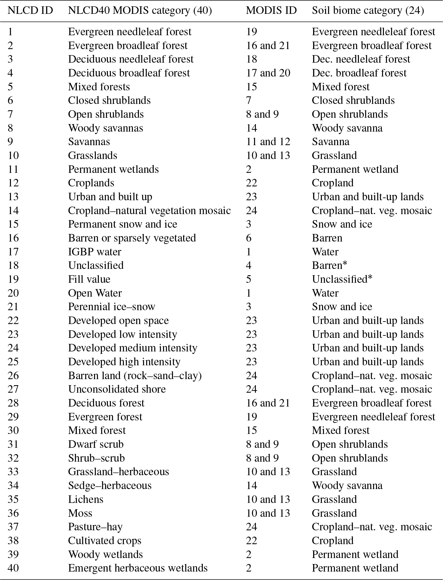
* NLCD categories 18 and 19 were mapped as MODIS category 1 (water) in Rasool et al. (2016), which have been corrected here.
Table A3Microbial ∕ organic biomass C and N % and % mapped to the respective NLCD40 MODIS land cover categories based on Xu et al. (2013) estimates.
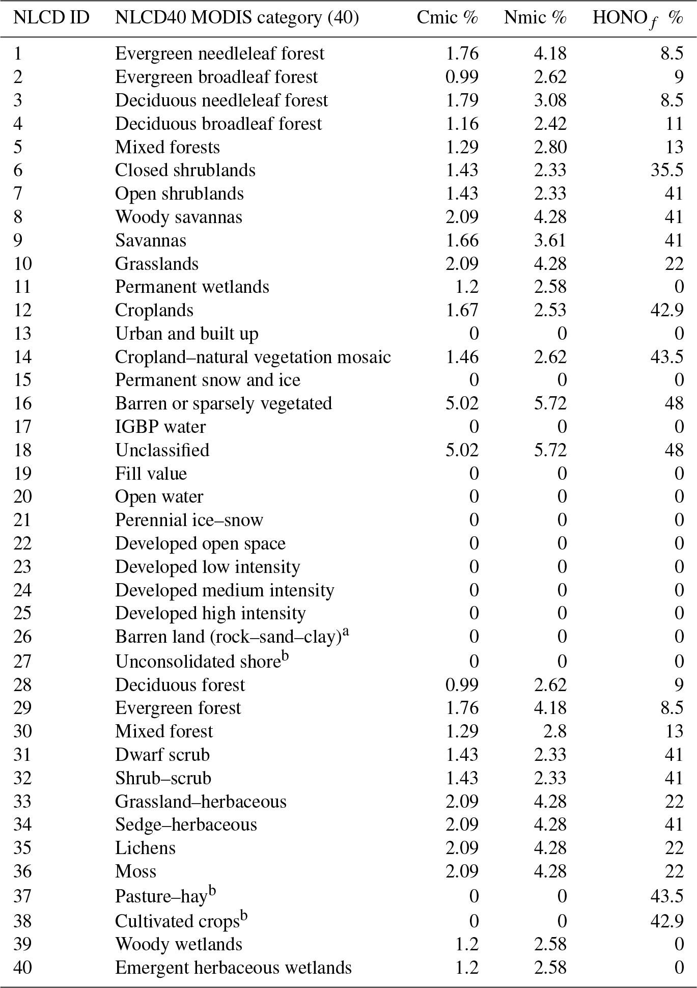
a NLCD classes 26 and 27 consisting of mostly rocks. b Cmic and Nmic for US croplands classified under NLCD classes 37 and 38 are kept as zero to prevent double counting, as they are accounted for by EPIC N data.
The supplement related to this article is available online at: https://doi.org/10.5194/gmd-12-849-2019-supplement.
QZR developed the model code with JOB. QZR performed the simulations and analysis. QZR prepared the paper with extensive reviews and edits from JOB and DSC.
The authors declare that they have no conflict of interest.
NASA (grant number NNX15AN63G) provided the funding for this work. We
acknowledge Ellen Cooter from the U.S. EPA for her insights and invaluable
help with EPIC/FEST-C modeling. The views expressed in this article are
those of the authors and do not necessarily reflect the views or policies of
the U.S. Environmental Protection Agency.
Edited by: Gerd A. Folberth
Reviewed by: two anonymous referees
Appel, K. W., Napelenok, S. L., Foley, K. M., Pye, H. O. T., Hogrefe, C., Luecken, D. J., Bash, J. O., Roselle, S. J., Pleim, J. E., Foroutan, H., Hutzell, W. T., Pouliot, G. A., Sarwar, G., Fahey, K. M., Gantt, B., Gilliam, R. C., Heath, N. K., Kang, D., Mathur, R., Schwede, D. B., Spero, T. L., Wong, D. C., and Young, J. O.: Description and evaluation of the Community Multiscale Air Quality (CMAQ) modeling system version 5.1, Geosci. Model Dev., 10, 1703–1732, https://doi.org/10.5194/gmd-10-1703-2017, 2017.
Barton, L., McLay, C., Schipper, L., and Smith, C.: Annual denitrification rates in agricultural and forest soils: a review, Soil Res., 37, 1073–1094, 1999.
Bash, J. O., Baker, K. R., and Beaver, M. R.: Evaluation of improved land use and canopy representation in BEIS v3.61 with biogenic VOC measurements in California, Geosci. Model Dev., 9, 2191–2207, https://doi.org/10.5194/gmd-9-2191-2016, 2016.
Bash, J. O., Cooter, E. J., Dennis, R. L., Walker, J. T., and Pleim, J. E.: Evaluation of a regional air-quality model with bidirectional NH3 exchange coupled to an agroecosystem model, Biogeosciences, 10, 1635–1645, https://doi.org/10.5194/bg-10-1635-2013, 2013.
Bertram, T. H., Cohen, R. C., Thorn III, W. J., and Chu, P. M.: Consistency of ozone and nitrogen oxides standards at tropospherically relevant mixing ratios, J. Air Waste Manage., 55, 1473–1479, 2005.
Bey, I., Jacob, D. J., Yantosca, R. M., Logan, J. A., Field, B., Fiore, A. M., Li, Q., Liu, H., Mickley, L. J., and Schultz, M.: Global modeling of tropospheric chemistry with assimilated meteorology: Model description and evaluation, J. Geophys. Res., 106, 23073–23096, 2001.
Bucsela, E. J., Krotkov, N. A., Celarier, E. A., Lamsal, L. N., Swartz, W. H., Bhartia, P. K., Boersma, K. F., Veefkind, J. P., Gleason, J. F., and Pickering, K. E.: A new stratospheric and tropospheric NO2 retrieval algorithm for nadir-viewing satellite instruments: applications to OMI, Atmos. Meas. Tech., 6, 2607–2626, https://doi.org/10.5194/amt-6-2607-2013, 2013.
Butterbach-Bahl, K., Baggs, E. M., Dannenmann, M., Kiese, R., and Zechmeister-Boltenstern, S.: Nitrous oxide emissions from soils: how well do we understand the processes and their controls?, Philos. T. R. Soc. B, 368, 20130122, https://doi.org/10.1098/rstb.2013.0122, 2013.
Cameron, K., Di, H. J., and Moir, J.: Nitrogen losses from the soil/plant system: a review, Ann. Appl. Biol., 162, 145–173, 2013.
Cao, P., Lu, C., and Yu, Z.: Agricultural nitrogen fertilizer uses in the continental US during 1850–2015: a set of gridded time-series data, PANGAEA, https://doi.org/10.1594/PANGAEA.883585, 2017.
Conrad, R.: Microbiological and biochemical background of production and consumption of NO and N2O in soil, in: Trace gas exchange in forest ecosystems, Springer, 2002.
Cooper, O. R., Parrish, D. D., Ziemke, J., Balashov, N. V., Cupeiro, M., Galbally, I. E., Gilge, S., Horowitz, L., Jensen, N. R., Lamarque, J. F., and Naik, V.: Global distribution and trends of tropospheric ozone: An observation-based review, Elementa, 2, https://doi.org/10.12952/journal.elementa.000029, 2014.
Cooter, E. J., Bash, J. O., Benson, V., and Ran, L.: Linking agricultural crop management and air quality models for regional to national-scale nitrogen assessments, Biogeosciences, 9, 4023–4035, https://doi.org/10.5194/bg-9-4023-2012, 2012.
Davidson, E. A. and Verchot, L. V.: Testing the Hole-in-the-Pipe Model of nitric and nitrous oxide emissions from soils using the TRAGNET Database, Global Biogeochem. Cy., 14, 1035–1043, 2000.
Davidson, E. and Kingerlee, W.: A global inventory of nitric oxide emissions from soils, Nutr. Cycl. Agroecosys., 48, 37–50, https://doi.org/10.1023/A:1009738715891, 1997.
Davidson, E. A., David, M. B., Galloway, J. N., Goodale, C. L., Haeuber, R., Harrison, J. A., Howarth, R.W., Jaynes, D. B., Lowrance, R. R., Nolan, B. T., Peel, J. L., Pinder, R. W., Porter, E., Snyder, C. S., Townsend, A. R., and Ward, M. H.: Excess nitrogen in the U.S. environment: trends, risks, and solutions, Issues in Ecology, Report Number 15, Ecological Society of America, 1–16, 2012.
Davidson, E.: Pulses of nitric oxide and nitrous oxide flux following wetting of dry soil: an assessment of probable sources and importance relative to annual fluxes, Ecol. Bull., 42, 149–155, 1992.
Del Grosso, S., Parton, W., Mosier, A., Ojima, D., Kulmala, A., and Phongpan, S.: General model for N2O and N2 gas emissions from soils due to dentrification, Global Biogeochem. Cy., 14, 1045–1060, 2000.
Evans, S. E. and Burke, I. C.: Carbon and nitrogen decoupling under an 11-year drought in the shortgrass steppe, Ecosystems, 16, 20–33, 2013.
Firestone, M. K. and Davidson, E. A.: Microbiological basis of NO and N2O production and consumption in soil, Life Sci. R., 47, 7–21, 1989.
Frink, C. R., Waggoner, P. E., and Ausubel, J. H.: Nitrogen fertilizer: retrospect and prospect, P. Natl. Acad. Sci. USA, 96, 1175–1180, 1999.
Gaillard, R. K., Jones, C. D., Ingraham, P., Collier, S., Izaurralde, R. C., Jokela, W., Osterholz, W., Salas, W., Vadas, P., and Ruark, M.: Underestimation of N2O emissions in a comparison of the DayCent, DNDC, and EPIC models, Ecol. Appl., 28, 694–708, 2018.
Geddes, J. A., Heald, C. L., Silva, S. J., and Martin, R. V.: Land cover change impacts on atmospheric chemistry: simulating projected large-scale tree mortality in the United States, Atmos. Chem. Phys., 16, 2323–2340, https://doi.org/10.5194/acp-16-2323-2016, 2016.
Gödde, M. and Conrad, R.: Influence of soil properties on the turnover of nitric oxide and nitrous oxide by nitrification and denitrification at constant temperature and moisture, Biol. Fert. Soils, 32, 120–128, 2000.
Gollehon, N. R., Caswell, M., Ribaudo, M., Kellogg, R. L., Lander, C., and Letson, D.: Confined Animal Production and Manure Nutrients. Washington, DC, U.S. Department of Agriculture, Economic Research Service, Agriculture Information Bulletin 771, available at: https://ageconsearch.umn.edu/record/33763 (last access: 22 February 2019), 2001.
Griffis, T. J., Chen, Z., Baker, J. M., Wood, J. D., Millet, D. B., Lee, X., Venterea, R. T., and Turner, P. A.: Nitrous oxide emissions are enhanced in a warmer and wetter world, P. Natl. Acad. Sci. USA, 114, 12081–12085, 2017.
Heil, J., Vereecken, H., and Brüggemann, N.: A review of chemical reactions of nitrification intermediates and their role in nitrogen cycling and nitrogen trace gas formation in soil, Eur. J. Soil Sci., 67, 23–39, 2016.
Hickman, J. E., Wu, S., Mickley, L. J., and Lerdau, M. T.: Kudzu (Pueraria montana) invasion doubles emissions of nitric oxide and increases ozone pollution, P. Natl. Acad. Sci. USA, 107, 10115–10119, 2010.
Holmes, N. S.: A review of particle formation events and growth in the atmosphere in the various environments and discussion of mechanistic implications, Atmos. Environ., 41, 2183–2201, 2007.
Homyak, P. M. and Sickman, J. O.: Influence of soil moisture on the seasonality of nitric oxide emissions from chaparral soils, Sierra Nevada, California, USA, J. Arid Environ., 103, 46–52, 2014.
Homyak, P. M., Blankinship, J. C., Marchus, K., Lucero, D. M., Sickman, J. O., and Schimel, J. P.: Aridity and plant uptake interact to make dryland soils hotspots for nitric oxide (NO) emissions, P. Natl. Acad. Sci. USA, 113, E2608–E2616, 2016.
Houlton, B., Morford, S., and Dahlgren, R.: Convergent evidence for widespread rock nitrogen sources in Earth's surface environment, Science, 360, 58–62, 2018.
Hu, H. W., Chen, D., and He, J. Z.: Microbial regulation of terrestrial nitrous oxide formation: Understanding the biological pathways for prediction of emission rates, FEMS Microbiol. Rev., 39, 729–749, 2015.
Hudman, R. C., Moore, N. E., Mebust, A. K., Martin, R. V., Russell, A. R., Valin, L. C., and Cohen, R. C.: Steps towards a mechanistic model of global soil nitric oxide emissions: implementation and space based-constraints, Atmos. Chem. Phys., 12, 7779–7795, https://doi.org/10.5194/acp-12-7779-2012, 2012.
Hudman, R. C., Russell, A. R., Valin, L. C., and Cohen, R. C.: Interannual variability in soil nitric oxide emissions over the United States as viewed from space, Atmos. Chem. Phys., 10, 9943–9952, https://doi.org/10.5194/acp-10-9943-2010, 2010.
Hutchinson, G. and Brams, E.: NO versus N2O emissions from an -amended Bermuda grass pasture, J. Geophys. Res.-Atmos., 97, 9889–9896, 1992.
IPCC: Climate Change 2013: The Physical Science Basis, Working Group I Contribution to the Fifth Assessment Report of the Intergovernmental Panel on Climate Change, edited by: Stocker, T. F., Qin, D., Plattner, G.-K., Tignor, M., Allen, S. K., Boschung, J., Nauels, A. Xia, Y., Bex, V., and Midgley, P. M., Cambridge University Press, Cambridge, UK, 2013.
Izaurralde, R. C., McGill, W. B., Williams, J. R., Jones, C. D., Link, R. P., Manowitz, D. H., Schwab, D. E., Zhang, X., Robertson, G. P., and Millar, N.: Simulating microbial denitrification with EPIC: Model description and evaluation, Ecol. Model., 359, 349–362, 2017.
Izaurralde, R. C., McGill, W. B., and Williams, J.: Development and application of the EPIC model for carbon cycle, greenhouse gas mitigation, and biofuel studies, in: Managing Agricultural Greenhouse Gases, Elsevier, 2012.
Izaurralde, R., Williams, J. R., Mcgill, W. B., Rosenberg, N. J., and Jakas, M. Q.: Simulating soil C dynamics with EPIC: Model description and testing against long-term data, Ecol. Model., 192, 362–384, 2006.
Jaeglé, L., Martin, R. V., Chance, K., Steinberger, L., Kurosu, T. P., Jacob, D. J., Modi, A. I., Yoboué, V., Sigha-Nkamdjou, L., and Galy-Lacaux, C.: Satellite mapping of rain-induced nitric oxide emissions from soils, J. Geophys. Res.-Atmos., 109, D21310, https://doi.org/10.1029/2004JD004787, 2004.
Jaeglé, L., Steinberger, L., Martin, R. V., and Chance, K.: Global partitioning of NOx sources using satellite observations: Relative roles of fossil fuel combustion, biomass burning and soil emissions, Faraday Discuss., 130, 407–423, 2005.
Jiang, Z., McDonald, B. C., Worden, H., Worden, J. R., Miyazaki, K., Qu, Z., Henze, D. K., Jones, D. B., Arellano, A. F., and Fischer, E. V.: Unexpected slowdown of US pollutant emission reduction in the past decade, P. Natl. Acad. Sci. USA, 115, 201801191, https://doi.org/10.1073/pnas.1801191115, 2018.
Kampa, M. and Castanas, E.: Human health effects of air pollution, Environ. Pollut., 151, 362–367, 2008.
Kellogg, R. L., Lander, C. H., Moffitt, D. C., and Gollehon, N.: Manure nutrients relative to the capacity of cropland and pastureland to assimilate nutrients: Spatial and temporal trends for the United States, Proceedings of the Water Environment Federation, 2000, 18–157, 2000.
Kesik, M., Blagodatsky, S., Papen, H., and Butterbach-Bahl, K.: Effect of pH, temperature and substrate on N2O, NO and CO2 production by Alcaligenes faecalis p, J. Appl. Microbiol., 101, 655–667, 2006.
Kim, H. C., Lee, P., Judd, L., Pan, L., and Lefer, B.: OMI NO2 column densities over North American urban cities: the effect of satellite footprint resolution, Geosci. Model Dev., 9, 1111–1123, https://doi.org/10.5194/gmd-9-1111-2016, 2016.
Kottek, M., Grieser, J., Beck, C., Rudolf, B., and Rubel, F.: World Map of the Köppen-Geiger climate classification updated, Meteorol. Z., 15, 259–263, https://doi.org/10.1127/0941-2948/2006/0130, 2006.
Kwok, R., Napelenok, S., and Baker, K.: Implementation and evaluation of PM2.5 source contribution analysis in a photochemical model, Atmos. Environ., 80, 398–407, 2013.
Lamsal, L. N., Krotkov, N. A., Celarier, E. A., Swartz, W. H., Pickering, K. E., Bucsela, E. J., Gleason, J. F., Martin, R. V., Philip, S., Irie, H., Cede, A., Herman, J., Weinheimer, A., Szykman, J. J., and Knepp, T. N.: Evaluation of OMI operational standard NO2 column retrievals using in situ and surface-based NO2 observations, Atmos. Chem. Phys., 14, 11587–11609, https://doi.org/10.5194/acp-14-11587-2014, 2014.
Laville, P., Lehuger, S., Loubet, B., Chaumartin, F., and Cellier, P.: Effect of management, climate and soil conditions on N2O and NO emissions from an arable crop rotation using high temporal resolution measurements, Agr. Forest Meteorol., 151, 228–240, 2011.
Leitner, S., Homyak, P. M., Blankinship, J. C., Eberwein, J., Jenerette, G. D., Zechmeister-Boltenstern, S., and Schimel, J. P.: Linking NO and N2O emission pulses with the mobilization of mineral and organic N upon rewetting dry soils, Soil Biol. Biochem., 115, 461–466, 2017.
Li, Y., Schichtel, B. A., Walker, J. T., Schwede, D. B., Chen, X., Lehmann, C. M., Puchalski, M. A., Gay, D. A., and Collett, J. L.: Increasing importance of deposition of reduced nitrogen in the United States, P. Natl. Acad. Sci. USA, 113, 5874–5879, 2016.
Liu, B., Mørkved, P. T., Frostegård, Å., and Bakken, L. R.: Denitrification gene pools, transcription and kinetics of NO, N2O and N2 production as affected by soil pH, FEMS Microbiol. Ecol., 72, 407–417, 2010.
Liu, X., Ju, X., Zhang, Y., He, C., Kopsch, J., and Fusuo, Z.: Nitrogen deposition in agroecosystems in the Beijing area, Agriculture, Ecosystems & Environment, 113, 370–377, 2006.
Lu, C. and Tian, H.: Global nitrogen and phosphorus fertilizer use for agriculture production in the past half century: shifted hot spots and nutrient imbalance, Earth Syst. Sci. Data, 9, 181–192, https://doi.org/10.5194/essd-9-181-2017, 2017.
Ludwig, J., Meixner, F., Vogel, B., and Förstner, J.: Soil-air exchange of nitric oxide: an overview of processes, environmental factors, and modeling studies, Biogeochemistry, 52, 225–257, https://doi.org/10.1023/A:1006424330555, 2001.
Machefert, S. E., Dise, N. B., Goulding, K. W. T., and Whitehead, P. G.: Nitrous oxide emission from a range of land uses across Europe, Hydrol. Earth Syst. Sci., 6, 325–338, https://doi.org/10.5194/hess-6-325-2002, 2002.
Maljanen, M., Yli-Pirilä, P., Hytönen, J., Joutsensaari, J., and Martikainen, P. J.: Acidic northern soils as sources of atmospheric nitrous acid (HONO), Soil Biol. Biochem., 67, 94–97, 2013.
Malm, W. C., Sisler, J. F., Huffman, D., Eldred, R. A., and Cahill, T. A.: Spatial and seasonal trends in particle concentration and optical extinction in the United States, J. Geophys. Res.-Atmos., 99, 1347–1370, 1994.
Mamtimin, B., Meixner, F. X., Behrendt, T., Badawy, M., and Wagner, T.: The contribution of soil biogenic NO and HONO emissions from a managed hyperarid ecosystem to the regional NOx emissions during growing season, Atmos. Chem. Phys., 16, 10175–10194, https://doi.org/10.5194/acp-16-10175-2016, 2016.
Manzoni, S. and Porporato, A.: Soil carbon and nitrogen mineralization: theory and models across scales, Soil Biol. Biochem., 41, 1355–1379, 2009.
Martin, R. E., Scholes, M., Mosier, A., Ojima, D., Holland, E., and Parton, W.: Controls on annual emissions of nitric oxide from soils of the Colorado shortgrass steppe, Global Biogeochem. Cy., 12, 81–91, 1998.
Medinets, S., Skiba, U., Rennenberg, H., and Butterbach-Bahl, K.: A review of soil NO transformation: Associated processes and possible physiological significance on organisms, Soil Biol. Biochem., 80, 92–117, 2015.
Moldrup, P., Olesen, T., Yoshikawa, S., Komatsu, T., and Rolston, D. E.: Three-porosity model for predicting the gas diffusion coefficient in undisturbed soil, Soil Sci. Soc. Am. J., 68, 750–759, 2004.
Montes, F., Meinen, R., Dell, C., Rotz, A., Hristov, A., Oh, J., Waghorn, G., Gerber, P., Henderson, B., and Makkar, H.: SPECIAL TOPICS – mitigation of methane and nitrous oxide emissions from animal operations: II. A review of manure management mitigation options, J. Anim. Sci., 91, 5070–5094, 2013.
Necpálová, M., Anex, R. P., Fienen, M. N., Del Grosso, S. J., Castellano, M. J., Sawyer, J. E., Iqbal, J., Pantoja, J. L., and Barker, D. W.: Understanding the DayCent model, Environ. Modell. Softw., 66, 110–130, 2015.
Neira, M.: The 2014 WHO conference on health and climate, SciELO Public Health, https://doi.org/10.2471/BLT.14.14389125177064, 2014.
Nemitz, E., Milford, C., and Sutton, M. A.: A two–layer canopy compensation point model for describing bi-directional biosphere–atmosphere exchange of ammonia, Q. J. Roy. Meteor. Soc., 127, 815–833, 2001.
Oikawa, P., Ge, C., Wang, J., Eberwein, J., Liang, L., Allsman, L., Grantz, D., and Jenerette, G.: Unusually high soil nitrogen oxide emissions influence air quality in a high-temperature agricultural region, Nat. Commun., 6, 8753, https://doi.org/10.1038/ncomms9753, 2015.
Oswald, R., Behrendt, T., Ermel, M., Wu, D., Su, H., Cheng, Y., Breuninger, C., Moravek, A., Mougin, E., Delon, C., Loubet, B., Pommerening-Röser, A., Sörgel, M., Pöschl, U., Hoffmann, T., Andreae, M. O., Meixner, F. X., and Trebs, I.: HONO emissions from soil bacteria as a major source of atmospheric reactive nitrogen, Science, 341, 1233–1235, https://doi.org/10.1126/science.1242266,2013.
Otte, T. L. and Pleim, J. E.: The Meteorology-Chemistry Interface Processor (MCIP) for the CMAQ modeling system: updates through MCIPv3.4.1, Geosci. Model Dev., 3, 243–256, https://doi.org/10.5194/gmd-3-243-2010, 2010.
Parrish, D., Williams, E., Fahey, D., Liu, S., and Fehsenfeld, F.: Measurement of nitrogen oxide fluxes from soils: Intercomparison of enclosure and gradient measurement techniques, J. Geophys. Res.-Atmos., 92, 2165–2171, 1987.
Parton, W. J., Holland, E. A., Del Grosso, S. J., Hartman, M. D., Martin, R. E., Mosier, A. R., Ojima, D. S., and Schimel, D. S.: Generalized model for NOx and N2O emissions from soils, J. Geophys. Res.-Atmos., 106, 17403–17419, https://doi.org/10.1029/2001JD900101, 2001.
Parton, W. J., Ojima, D. S., Cole, C. V., and Schimel, D. S.: A general model for soil organic matter dynamics: sensitivity to litter chemistry, texture and management, SSSA Spec. Publ., 1994, 147–167, 1994.
Pilegaard, K.: Processes regulating nitric oxide emissions from soils, Philos. T. Roy. Soc. B, 368, 1621, https://doi.org/10.1098/rstb.2013.0126, 2013.
Pleim, J. E. and Xiu, A.: Development of a land surface model. Part II: Data assimilation, J. Appl. Meteorol., 42, 1811–1822, 2003.
Pleim, J. E., Bash, J. O., Walker, J. T., and Cooter, E. J.: Development and evaluation of an ammonia bidirectional flux parameterization for air quality models, J. Geophys. Res., 118, 3794–3806, https://doi.org/10.1002/jgrd.50262, 2013.
Pope, C. A., Burnett, R. T., Krewski, D., Jerrett, M., Shi, Y., Calle, E. E., and Thun, M. J.: Cardiovascular mortality and exposure to airborne fine particulate matter and cigarette smoke: shape of the exposure-response relationship, Circulation, 120, 941–948, 2009.
Potter, P., Navin, R., Elena, M. B., and Simon D. D.: Characterizing the spatial patterns of global fertilizer application and manure production, Earth Interact., 14, 1–22, 2010.
Pouliot, G. and Pierce, T.: Integration of the Model of Emissionsof Gases and Aerosols from Nature (MEGAN) into the CMAQModeling System, 18th International Emission Inventory Conference, Baltimore, Maryland, 14–17 April 2009.
Pusede, S. E. and Cohen, R. C.: On the observed response of ozone to NOx and VOC reactivity reductions in San Joaquin Valley California 1995–present, Atmos. Chem. Phys., 12, 8323–8339, https://doi.org/10.5194/acp-12-8323-2012, 2012.
Rasool, Q. Z., Zhang, R., Lash, B., Cohan, D. S., Cooter, E. J., Bash, J. O., and Lamsal, L. N.: Enhanced representation of soil NO emissions in the Community Multiscale Air Quality (CMAQ) model version 5.0.2, Geosci. Model Dev., 9, 3177–3197, https://doi.org/10.5194/gmd-9-3177-2016, 2016.
Rasool, Q. Z., Bash, J. O., and Cohan, D. S.: Mechanistic representation of soil nitrogen emissions in CMAQ version 5.1, ORNL DAAC, Oak Ridge, Tennessee, USA, https://doi.org/10.3334/ORNLDAAC/1661, 2018.
Redding, M., Shorten, P., Lewis, R., Pratt, C., Paungfoo-Lonhienne, C., and Hill, J.: Soil N availability, rather than N deposition, controls indirect N2O emissions, Soil Biol. Biochem., 95, 288–298, 2016.
Ribaudo, M., Key, N., and Sneeringer, S.: The potential role for a nitrogen compliance policy in mitigating Gulf hypoxia, Appl. Econ. Perspect. P., 39, 458–478, 2016.
Ribaudo, M., Livingston, M., and Williamson, J.: Nitrogen management on us corn acres, 2001-10, United States Department of Agriculture, Economic Research Service, 2012.
Ribaudo, M., Gollehon, N., and Agapoff, J.: Land application of manure by animal feeding operations: Is more land needed?, J. Soil Water Conserv., 58, 30–38, 2003.
Robertson, G. P. and Groffman, P.: Nitrogen transformations, in: Soil Microbiology, Ecology and Biochemistry, 3rd Edn., Elsevier, 2007.
Romer, P. S., Duffey, K. C., Wooldridge, P. J., Edgerton, E., Baumann, K., Feiner, P. A., Miller, D. O., Brune, W. H., Koss, A. R., de Gouw, J. A., Misztal, P. K., Goldstein, A. H., and Cohen, R. C.: Effects of temperature-dependent NOx emissions on continental ozone production, Atmos. Chem. Phys., 18, 2601–2614, https://doi.org/10.5194/acp-18-2601-2018, 2018.
Schimel, J. P. and Weintraub, M. N.: The implications of exoenzyme activity on microbial carbon and nitrogen limitation in soil: a theoretical model, Soil Biol. Biochem., 35, 549–563, 2003.
Schindlbacher, A., Zechmeister-Boltenstern, S., and Butterbach-Bahl, K.: Effects of soil moisture and temperature on NO, NO2, and N2O emissions from European forest soils, J. Geophys. Res.-Atmos., 109, 17302–17309, 2004.
Scholes, M., Martin, R., Scholes, R., Parsons, D., and Winstead, E.: NO and N2O emissions from savanna soils following the first simulated rains of the season, Nutr. Cycl. Agroecosys., 48, 115– 122, https://doi.org/10.1023/A:1009781420199, 1997.
Seinfeld, J. H. and Pandis, S. N.: Atmospheric chemistry and physics: from air pollution to climate change, John Wiley & Sons, 2012.
Simon, H., Reff, A., Wells, B., Xing, J., and Frank, N.: Ozone trends across the United States over a period of decreasing NOx and VOC emissions, Environ. Sci. Technol., 49, 186–195, 2014.
Skamarock, W. C., Klemp, J. B., Dudhia, J., Gill, D. O., Barker, D. M., Duda, M. G., Huang, X., Wang, W., and Powers, J. G.: A description of the advanced research WRF version 3, NCAR Tech. Note, NCAR/TN-475+STR, 8 pp., Natl. Cent. for Atmos. Res., Boulder, Colo., available at: http://www.mmm.ucar.edu/wrf/users/docs/arw_v3.pdf (last access: 22 February 2019), 2008.
Stehfest, E. and Bouwman, L.: N2O and NO emission from agricultural fields and soils under natural vegetation: summarizing available measurement data and modeling of global annual emissions, Nutr. Cycl. Agroecosys., 74, 207–228, https://doi.org/10.1007/s10705-006-9000-7, 2006.
Steinkamp, J. and Lawrence, M. G.: Improvement and evaluation of simulated global biogenic soil NO emissions in an AC-GCM, Atmos. Chem. Phys., 11, 6063–6082, https://doi.org/10.5194/acp-11-6063-2011, 2011.
Strode, S. A., Rodriguez, J. M., Logan, J. A., Cooper, O. R., Witte, J. C., Lamsal, L. N., Damon, M., Van Aartsen, B., Steenrod, S. D., and Strahan, S. E.: Trends and variability in surface ozone over the United States, J. Geophys. Res.-Atmos., 120, 9020–9042, https://doi.org/10.1002/2014JD022784, 2015.
Su, H., Cheng, Y., Oswald, R., Behrendt, T., Trebs, I., Meixner, F. X., Andreae, M. O., Cheng, P., Zhang, Y., and Pöschl, U.: Soil nitrite as a source of atmospheric HONO and OH radicals, Science, 333, 1616–1618, 2011.
Tilman, D., Fargione, J., Wolff, B., D'antonio, C., Dobson, A., Howarth, R., Schindler, D., Schlesinger, W. H., Simberloff, D., and Swackhamer, D.: Forecasting agriculturally driven global environmental change, Science, 292, 281–284, 2001.
Townsend, A. R., Howarth, R. W., Bazzaz, F. A., Booth, M. S., Cleveland, C. C., Collinge, S. K., Dobson, A. P., Epstein, P. R., Holland, E. A., and Keeney, D. R.: Human health effects of a changing global nitrogen cycle, Front. Ecol. Environ., 1, 240–246, 2003.
Travis, K. R., Jacob, D. J., Fisher, J. A., Kim, P. S., Marais, E. A., Zhu, L., Yu, K., Miller, C. C., Yantosca, R. M., Sulprizio, M. P., Thompson, A. M., Wennberg, P. O., Crounse, J. D., St. Clair, J. M., Cohen, R. C., Laughner, J. L., Dibb, J. E., Hall, S. R., Ullmann, K., Wolfe, G. M., Pollack, I. B., Peischl, J., Neuman, J. A., and Zhou, X.: Why do models overestimate surface ozone in the Southeast United States?, Atmos. Chem. Phys., 16, 13561–13577, https://doi.org/10.5194/acp-16-13561-2016, 2016.
Venterea, R. T. and Rolston, D. E.: Mechanisms and kinetics of nitric and nitrous oxide production during nitrification in agricultural soil, Glob. Change Biol., 6, 303–316, 2000.
Vinken, G. C. M., Boersma, K. F., Maasakkers, J. D., Adon, M., and Martin, R. V.: Worldwide biogenic soil NOx emissions inferred from OMI NO2 observations, Atmos. Chem. Phys., 14, 10363–10381, https://doi.org/10.5194/acp-14-10363-2014, 2014.
Wade, T., Claassen, R. L., and Wallander, S.: Conservation-practice adoption rates vary widely by crop and region, United States Department of Agriculture, Economic Research Service, 2015.
Wang, C., Houlton, B. Z., Dai, W., and Bai, E.: Growth in the global N2 sink attributed to N fertilizer inputs over 1860 to 2000, Sci. Total Environ., 574, 1044–1053, 2017.
Wang, L., Xu, J., Yang, J., Zhao, X., Wei, W., Cheng, D., Pan, X., and Su, J.: Understanding haze pollution over the southern Hebei area of China using the CMAQ model, Atmos. Environ., 56, 69–79, 2012.
Wang, Y., Logan, J. A., and Jacob, D. J.: Global simulation of tropospheric O3-NOx-hydrocarbon chemistry: 2. Model evaluation and global ozone budget, J. Geophys. Res.-Atmos., 103, 10727–10755, 1998.
Wang, Y., Zhang, Q. Q., He, K., Zhang, Q., and Chai, L.: Sulfate-nitrate-ammonium aerosols over China: response to 2000–2015 emission changes of sulfur dioxide, nitrogen oxides, and ammonia, Atmos. Chem. Phys., 13, 2635–2652, https://doi.org/10.5194/acp-13-2635-2013, 2013.
Weier, K., Doran, J., Power, J., and Walters, D.: Denitrification and the dinitrogen/nitrous oxide ratio as affected by soil water, available carbon, and nitrate, Soil Sci. Soc. Am. J., 57, 66–72, 1993.
Williams, E. and Fehsenfeld, F.: Measurement of soil nitrogen oxide emissions at three North American ecosystems, J. Geophys. Res.-Atmos., 96, 1033–1042, 1991.
Williams, E. J., Guenther, A., and Fehsenfeld, F. C.: An inventory of nitric oxide emissions from soils in the United States, J. Geophys. Res., 97, 7511–7519, 1992.
Williams, J., Izaurralde, R., and Steglich, E.: Agricultural policy/environmental extender model, Theoretical Documentation, Version, 604, 2008–2017, 2008.
Xu, X., Thornton, P. E., and Post, W. M.: A global analysis of soil microbial biomass carbon, nitrogen and phosphorus in terrestrial ecosystems, Global Ecol. Biogeogr., 22, 737–749, 2013.
Xu, X., Thornton, P., and POTAPOV, P.: Compilation of Global Soil Microbial Biomass Carbon, Nitrogen, and Phosphorus Data, ORNL DAAC, Oak Ridge, Tennessee, USA, https://doi.org/10.3334/ORNLDAAC/1264, 2015.
Yienger, J. and Levy, H.: Empirical model of global soil-biogenic NOx emissions, J. Geophys. Res.-Atmos., 100, 11447–11464, 1995.
Zhu, L., Henze, D., Bash, J., Jeong, G.-R., Cady-Pereira, K., Shephard, M., Luo, M., Paulot, F., and Capps, S.: Global evaluation of ammonia bidirectional exchange and livestock diurnal variation schemes, Atmos. Chem. Phys., 15, 12823–12843, https://doi.org/10.5194/acp-15-12823-2015, 2015.