the Creative Commons Attribution 4.0 License.
the Creative Commons Attribution 4.0 License.
 | 07 Oct 2019
Pysteps: an open-source Python library for probabilistic precipitation nowcasting (v1.0)
Daniele Nerini
Andrés A. Pérez Hortal
Carlos Velasco-Forero
Alan Seed
Urs Germann
Loris Foresti
Pysteps is an open-source and community-driven Python library for probabilistic precipitation nowcasting, that is, very-short-range forecasting (0–6 h). The aim of pysteps is to serve two different needs. The first is to provide a modular and well-documented framework for researchers interested in developing new methods for nowcasting and stochastic space–time simulation of precipitation. The second aim is to offer a highly configurable and easily accessible platform for practitioners ranging from weather forecasters to hydrologists. In this sense, pysteps has the potential to become an important component for integrated early warning systems for severe weather.
The pysteps library supports various input/output file formats and implements several optical flow methods as well as advanced stochastic generators to produce ensemble nowcasts. In addition, it includes tools for visualizing and post-processing the nowcasts and methods for deterministic, probabilistic and neighborhood forecast verification. The pysteps library is described and its potential is demonstrated using radar composite images from Finland, Switzerland, the United States and Australia. Finally, scientific experiments are carried out to help the reader to understand the pysteps framework and sensitivity to model parameters.
- Article
(15250 KB) - Full-text XML
- BibTeX
- EndNote


As defined by the World Meteorological Organization (WMO), nowcasting encompasses a description of the current state of the atmosphere along with forecasts up to 6 h ahead (Wang et al., 2017). These short-term forecasts, typically obtained by extrapolation of observations, statistical models or numerical weather prediction (NWP), represent an essential tool to predict severe weather, such as heavy precipitation and intense thunderstorms.
Excessive rainfall can act as a trigger for water-related hazards (Alfieri et al., 2012), and this is particularly true in an increasingly urbanized territory or in the presence of steep topography. When vulnerable objects become exposed to such hazards, risk can manifest in terms of property damage and loss of lives.
Reliable precipitation nowcasts are therefore needed to support decision making during severe weather, for example, to decide whether to interrupt a train line exposed to debris flows or to evacuate buildings in flood-prone areas, as well as in the context of the optimization of airport operations and regulation of sewage systems during storm events. All such scenarios can benefit from the availability of real-time nowcasting systems that take into account the predictability of precipitation and related hazards at a high spatial and temporal resolution so that risk is mitigated.
1.1 From deterministic to probabilistic nowcasting
Weather radars are ideally suited for providing the input data for precipitation nowcasting at high resolution, namely spatial scales under 2 km and time ranges between 5 min and 3 h (Berne et al., 2004). Despite recent advances in numerical weather prediction (e.g., Sun et al., 2014), extrapolation-based nowcasting remains the primary approach at such space- and timescales, typically outperforming NWP forecasts in the first 2–5 h, depending on the weather situation, domain and NWP characteristics (e.g., Berenguer et al., 2012; Mandapaka et al., 2012; Simonin et al., 2017; Jacques et al., 2018). Other recent developments include machine learning methods, for which promising results have been obtained (e.g., Xingjian et al., 2015; Foresti et al., 2019), but these have not so far been deployed in operational nowcasting systems.
Precipitation exhibits variability over a wide range of space- and timescales (e.g., Lovejoy and Schertzer, 2013) which, in combination with the chaotic nature of the atmosphere (e.g., Lorenz, 1996), limits our ability to predict its evolution in a deterministic manner. The NWP community recognized this challenge in the early 1990s and tackled the problem by producing an ensemble of NWP forecasts by perturbing the set of initial conditions (e.g., Toth and Kalnay, 1997). Those perturbations grow exponentially and lead to an ensemble of solutions that reflect forecast uncertainties. The information contained in the ensemble can then be used to derive probabilistic forecasts.
Just as any other forecasting technique, the skill of radar-based nowcasting was found to depend on multiple factors such as the meteorological conditions, geographical location, spatial and temporal scales (e.g., Germann and Zawadzki, 2002; Foresti and Seed, 2014; Atencia et al., 2017; Mejsnar et al., 2018). It is therefore not surprising that also the nowcasting community rapidly acknowledged the importance of estimating predictive uncertainty (e.g., Seed, 2003; Germann and Zawadzki, 2004; Bowler et al., 2006). A common approach is based on stochastic simulation, in which correlated noise fields are used to perturb a deterministic nowcast (e.g., Bowler et al., 2006; Berenguer et al., 2011; Liguori and Rico-Ramirez, 2014; Foresti et al., 2016). Substantial research efforts have been made to make the perturbation fields as realistic as possible and consistent with the nowcast uncertainty (e.g., Seed et al., 2013; Nerini et al., 2017). For a review of the history of nowcasting starting from the 1950s, and its evolution to the probabilistic framework, we refer the reader to Pierce et al. (2012).
1.2 The pysteps open-source initiative
Similarly to other research fields, the nowcasting community has invested a significant amount of time to re-implement from scratch routines and algorithms that have been around for decades, for example, optical flow and advection schemes. Part of this problem is due to the unavailability of software, which is often proprietary or too poorly documented to be understood, trusted and used.
Recognizing that nowcasting methods and related applications can be further developed and distributed by promoting universal access to existing knowledge, a Python-based software package, called pysteps, is being developed as a community-driven effort. Such effort fits well into the weather radar community with emergence of open data and an increasing number of open-source software projects (Heistermann et al., 2015), for instance, in radar data processing (Heistermann et al., 2013; Helmus and Collis, 2016). More recently, community-based initiatives dedicated to nowcasting have emerged, for example, Com-SWIRLS by the Regional Specialized Meteorological Centre (RSMC) for Nowcasting operated by the Hong Kong Observatory (HKO), IMPROVER by the UK MetOffice or rainymotion at the University of Potsdam (see Table 1).
Wong et al. (2016)Flowerdew (2018)Haiden et al. (2011)Ayzel et al. (2019)Bowler et al. (2006)Seed et al. (2013)Table 1Non-exhaustive list (in alphabetical order) of precipitation nowcasting packages that are in principle available to the public. Open-source libraries have their source code available to the general public. Free-license libraries can be obtained upon request.
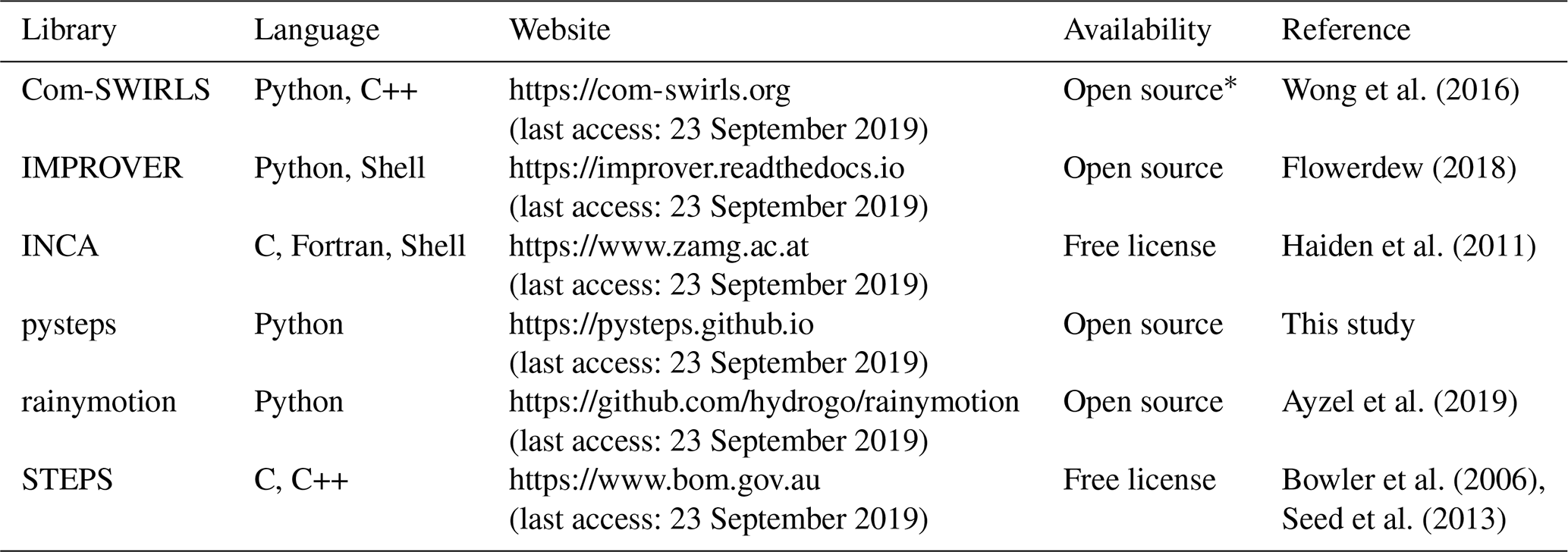
* Only for national meteorological and hydrological services within WMO.
In this article, we present pysteps, an open-source and community-driven Python library for probabilistic precipitation nowcasting. The objective of pysteps is two-fold. First, it aims at providing a well-documented and modular framework for development of new nowcasting methods. In this sense, pysteps promotes the adoption of open-science practices, as the lack of common standards, transparency, code availability and well-documented workflows in computational disciplines can lead to non-reproducible results, hence questioning their scientific value (Hutton et al., 2016). Second, pysteps aims at providing an easily accessible software package for practitioners ranging from weather forecasters to hydrologists.
1.3 Outline of the paper
The paper is structured as follows. The theoretical framework for precipitation nowcasting and using stochastic perturbations to characterize the uncertainty is formulated in Sect. 2. The general architecture of the pysteps library is presented in Sect. 3. A comprehensive verification of pysteps nowcasts is given in Sect. 4. Various experiments to understand the sensitivity of pysteps to the model parameters and define the default configuration are done in Sect. 5. The limits of pysteps are tested in Sect. 6 using a tropical cyclone and severe convection case in Australia. Section 7 concludes the paper and lists potential future applications of pysteps. Finally, code listings demonstrating the use of pysteps are given in Appendix A.
This section introduces the basic concepts and components of probabilistic nowcasting models based on the Lagrangian persistence of radar precipitation fields and describes how these are currently implemented in pysteps.
2.1 Lagrangian persistence and optical flow
In its simplest form, extrapolation-based precipitation nowcasting assumes that over the time frame of a few hours the evolution of precipitation can be captured by moving the radar echoes along a stationary motion field without changes in intensity. In the literature, this is known as Lagrangian persistence (Zawadzki et al., 1994).
Denoting a precipitation parcel by R and its displacement vector by α(τ), the conservation equation for an incompressible flow is written as
or equivalently in differential form as
where , and u and v are the x and y components of the motion field. In the so-called optical flow methods, u and v are estimated for a given location by solving Eq. (2) numerically based on a sequence of precipitation intensity fields. Typically, a constraint on the spatial continuity of nearby u and v is imposed to guarantee a unique solution. Once the motion field is known, the radar echoes are extrapolated by means of an advection scheme.
Three methods are currently implemented in pysteps for motion field estimation: a local Lucas–Kanade method (Lucas and Kanade, 1981; Bouguet, 2001), a global variational echo-tracking approach (Laroche and Zawadzki, 1994; Germann and Zawadzki, 2002) and a spectral approach (DARTS, Ruzanski et al., 2011). The currently implemented advection method is the backward-in-time semi-Lagrangian scheme described in Germann and Zawadzki (2002), which is robust against numerical diffusion.
2.2 Sources of uncertainty
The predictability of the atmosphere is intrinsically limited by the fact that its state cannot be observed with absolute precision nor expressed without approximations in its governing laws (Lorenz, 1996). In the case of radar-based precipitation nowcasting, predictive uncertainty originates from errors in the estimation of the current state of the rainfall and motion fields (initial state errors), and limitations of Lagrangian persistence as a model to predict the evolution of the rainfall and motion fields (model errors).
The main contribution to model errors in the Lagrangian approach stems from the evolution of precipitation in terms of initiation, growth, decay and termination processes that violate the steady-state assumption. Other sources of model uncertainty include the assumption of stationarity of the motion field, inaccuracies due to the practical implementation of the method, as the discretization in time, space and reflectivity, and numerical diffusion of the advection scheme (Germann et al., 2006b).
Currently, pysteps focuses on the representation of the model errors, whereas incorporation of the initial state errors in the nowcasting is left for future work.
2.3 Data transformation
The statistics of intermittent precipitation rates are non-Gaussian and display a typical asymmetric distribution that is bounded at zero. Such properties restrict the usage of well-established stochastic models that assume Gaussianity. A common workaround is to introduce a suitable data transformation to approximate a normal distribution (e.g., Erdin et al., 2012).
Currently, pysteps assumes a log-normal distribution of rain rates by applying the logarithmic transformation
that corresponds to logarithmic radar rain rates (units of dBR). The value of −15 dBR is equivalent to assigning a rain rate of approximately 0.03 mm h−1 to the zeros. Hereafter, R refers to the transformed rain rates, unless otherwise stated.
Using the logarithmic transformation is motivated by the fact that rain rates are approximately log-normally distributed (Crane, 1990). This has two main advantages. First, it simplifies the estimation of distribution parameters, particularly with limited sample size and in the presence of measurement noise (Harris et al., 1997). Second, the decomposition of log-transformed rainfall fields defines a multiplicative cascade, where multiplication is replaced with summation in the transformed space (Seed, 2003).
2.4 A cascade of spatial scales
It has been shown that the lifetime of precipitation relates to its spatial scale (e.g., Venugopal et al., 1999; Seed, 2003; Germann et al., 2006b), often denominated as dynamic scaling. Recognizing this fundamental property, Seed (2003) introduced the Spectral Prognosis (S-PROG) model, which laid the foundation for the development of Short-Term Ensemble Prediction System (STEPS) (Bowler et al., 2006; Seed et al., 2013). The key idea is to decompose the precipitation field into a multiplicative cascade, where the cascade levels represent different spatial scales, and treat them separately in the nowcasting model.
In STEPS, the scale decomposition is done by applying a fast Fourier transform (FFT) to the input precipitation field. This is motivated by the fact that for a grid of size L×L pixels, the radial Fourier wavenumbers are related to spatial scales via
where Δx denotes the grid resolution (km). Thus, the spatial scale is half the wavelength. Alternative approaches to perform a scale decomposition include the discrete-cosine transform (Germann and Zawadzki, 2002; Surcel et al., 2014) or wavelets (Turner et al., 2004; Scovell, 2018).
In the current implementation of pysteps, we adopt the approach of Pulkkinen et al. (2018), where Gaussian weight functions are used for separating the Fourier spectrum into a set of radial bands. An example of the weight functions for the domain covered by the Finnish Meteorological Institute (FMI) radars is shown in Fig. 1. After the FFT and Gaussian filtering, each frequency band is transformed back to the spatial domain, which results in a cascade with n levels each representing a different scale (see an example in Fig. 2).
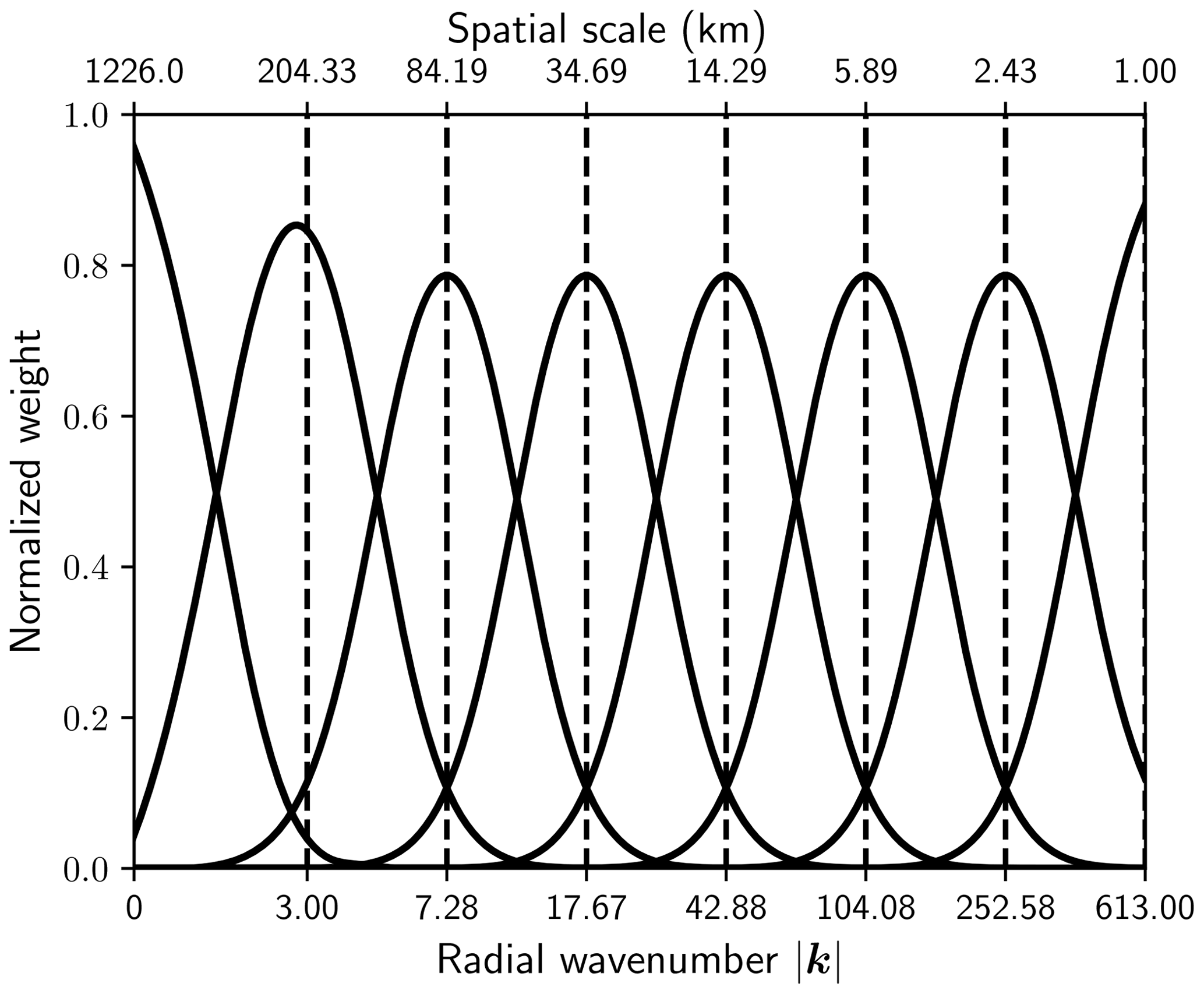
Figure 1Normalized weight functions with corresponding Fourier wavenumbers and spatial scales for the FMI domain. The domain is a 760×1226 grid at 1 km resolution.
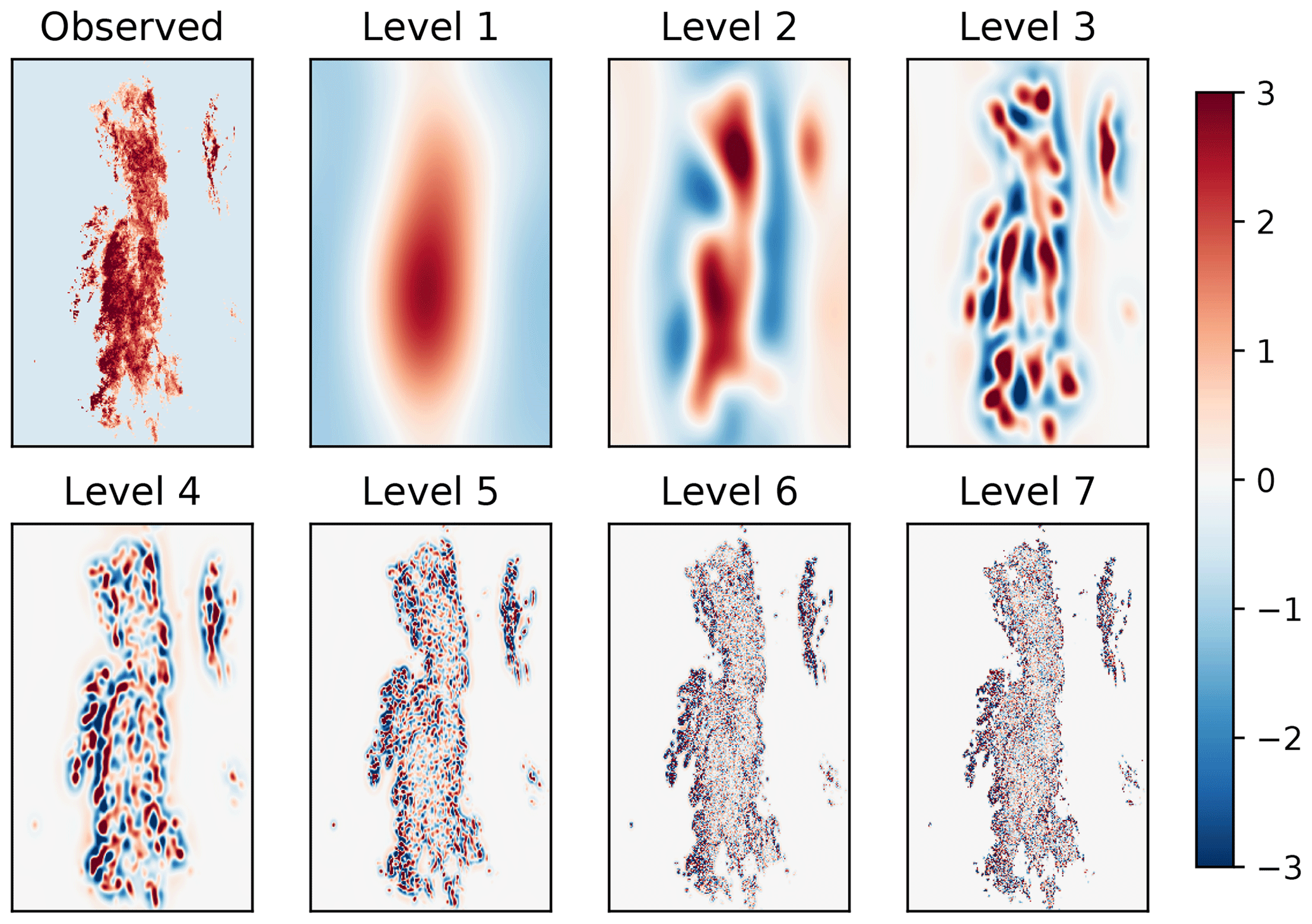
Figure 2The radar observations and seven first levels of the cascade decomposition of an FMI rain rate composite at 16:00 UTC on 28 September 2016. Values below −10 dBR were set to −15 dBR before applying the decomposition in order to reduce the discontinuity at the boundaries of precipitation areas. The observed field and the cascade levels have been normalized to zero mean and unit variance. See Listing A1 in Appendix A for obtaining the decomposition.
2.5 Temporal evolution
In nowcasting, the typical approach to model the temporal evolution of precipitation fields employs an auto-regressive (AR) process that combines the deterministic component from Lagrangian persistence with a stochastic innovation term, also referred to as a noise or perturbation term. For instance, S-PROG and STEPS use a second-order AR(2) process with two parameters. Separate AR(2) processes are applied to each cascade level to account for the dynamic scaling of precipitation. The combination of the auto-regressive model in time and the cascade model in space allows one to control the temporal evolution and correlation structure of precipitation.
Currently, a more general AR(p) model has been implemented in pysteps. For each cascade level j, the recursion formula is given by
The first term corresponds to the deterministic predictable component at cascade level j (i.e., Lagrangian persistence). The second term is a stochastic term that represents the unpredictable component at the same cascade level j, that is, mainly initiation, growth and decay of precipitation. The symbol Δt denotes the time difference between consecutive precipitation fields Rj that are normalized to zero mean and unit variance.
The parameters ϕj,k in the above model are estimated from time-lagged auto-correlation coefficients ρj,k for using the Yule–Walker equations (Hamilton, 1994). For p=2, the correlation coefficients can be adjusted to ensure that the resulting AR(p) process is stationary and non-periodic (Box et al., 2013). Finally, the parameters ϕj,0 are chosen as
Given that the variance of the noise fields εj is one, this choice guarantees that the AR(p) process is normalized to unit variance (Hamilton, 1994).
The theoretical auto-correlation function (ACF) of the AR(2) process can be computed recursively from the model parameters and auto-correlation coefficients (Chatfield, 2003) according to
The empirical ACF can be derived by computing the correlation coefficients between the extrapolation nowcasts and the observations.
For an exponentially decaying ACF, the precipitation lifetime is defined as the time when the ACF, theoretical or empirical, falls below the value , where e is the Euler number. Alternatively, one can estimate the lifetime by integrating the ACF according to
It is not common to employ an AR(p) process with p>2 for several reasons. First, it is not trivial to guarantee the stationarity and non-periodicity of the process. Second, when estimated in Lagrangian frame, the higher-order auto-correlation coefficients are affected by the uncertainty of the motion field. This occurs especially at small spatial scales as it is difficult to properly track convective cells over several time steps. Third, a low-order AR process is generally sufficient to model the loss of predictability in the nowcasting range; departures are usually observed only after ≈2 h (Atencia and Zawadzki, 2014).
2.6 Stochastic perturbations of precipitation intensities
The perturbation field ε in Eq. (5) is typically generated as a correlated Gaussian random field using FFT filtering (e.g., Pegram and Clothier, 2001; Bowler et al., 2006). The process consists of three steps:
-
generate a Gaussian white noise field,
-
apply the FFT and a Fourier filter to the above to generate a random field having the desired correlation structure and
-
apply the inverse FFT to transform the noise field back to the spatial domain.
This technique is also known as power–law filtering of white noise or fractional integration (Schertzer and Lovejoy, 1987).
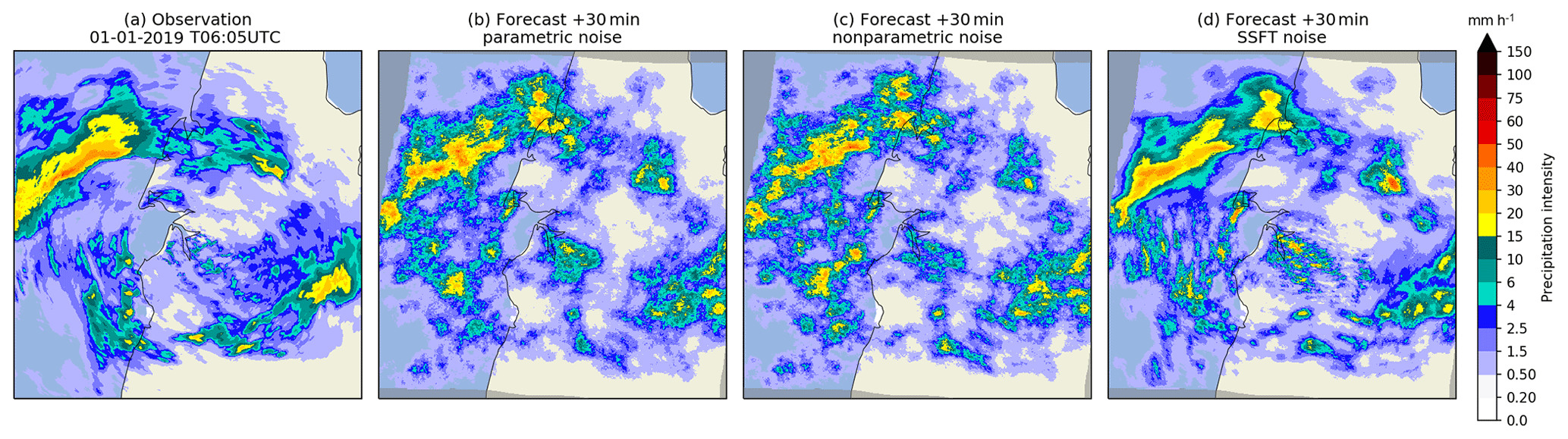
Figure 3Comparison of three +30 min stochastic nowcasts produced with the FFT noise generators available in pysteps as described in Sect. 2.6. (a) The radar-based rainfall analysis from the Australian radar network valid at 06:05 UTC on 1 January 2019 on a 512×512 pixel grid (event no. 2 in Table 10). (b)–(d) One member of a +30 min nowcast produced using (b) the parametric noise generator, (c) the non-parametric generator or (d) the short-space Fourier transform (SSFT) generator with a 128×128 pixel sliding window. All realizations share the same random seed.
At present, three methods for filtering white noise fields have been implemented in pysteps. In the absence of a model that predicts the evolution of the spatial correlation structure, one assumes that the correlation structure remains constant through the nowcast. An example is provided in Fig. 3.
In the parametric method introduced by Pegram and Clothier (2001), the filtered noise field ε is obtained from the white noise field εw as
where ℱ denotes the Fourier transform and the function f defines the slope of the radially averaged power spectrum (RAPS).
Our implementation follows the approach by Seed (2003), which uses a piecewise linear function with two spectral slopes (β1,β2) and one breaking point. The main limitation of such model relates to the assumption of an isotropic power–law scaling relationship, meaning that anisotropic structures such as rainfall bands cannot be represented.
In the non-parametric method (Seed et al., 2013), the Fourier filter is obtained directly from the power spectrum of the observed precipitation field R such that
Differently to the parametric method, the non-parametric approach allows generating perturbation fields with anisotropic structures. On the other hand, the approach requires a larger sample size and is sensitive to the quality of the input data, e.g., the presence of residual clutter in the radar image. In addition, both techniques assume spatial stationarity of the covariance structure of the field.
The third method is an extension of the non-parametric approach, where the noise field is generated locally to account for spatial inhomogeneities in the covariance structure of the rainfall field. The technique is based on the short-space Fourier transform (SSFT) and it is described in Nerini et al. (2017). Essentially, the non-parametric approach in Eq. (10) is localized in (x,y) by
where is the outer product of two Hanning windows of sizes n1 and n2 centered in (x,y).
2.7 Stochastic perturbations of the motion field
A second source of uncertainty in Lagrangian persistence nowcasting stems from temporal evolution of the motion field (Germann et al., 2006b). This can be accounted for by adding stochastic perturbations. In the current implementation of pysteps, this is done by applying the method of Bowler et al. (2006).
For simplicity, the perturbation field is assumed to be spatially constant for each ensemble member, but the magnitude of the perturbations increases with respect to lead time. For a given initial advection field w0 and lead time t, the perturbed velocities are given by
where and denote the components parallel and perpendicular to the initial advection field w0, respectively. The random variables (εpar and εperp) are sampled from the Laplace distribution with zero mean and unit variance. Scaling of the perturbations is done according to
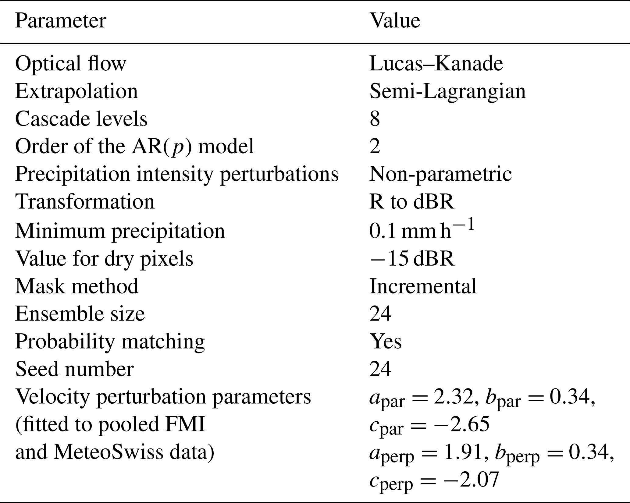
where the parameters are climatologically fitted by using a large sample of advection fields. Example values of these parameters can be found in Table 5.
2.8 Post-processing of nowcasts
To ensure that the forecast fields have the same statistical properties with the observed ones, post-processing is typically done at the very end of the chain. This is necessary because intermediate steps may introduce discrepancies. One major source of such discrepancies is related to the difficulty to model the intermittency of precipitation. Typically, the basic statistical properties such as wet-area ratio, mean, variance and the marginal distribution of precipitation intensities are assumed to remain invariant through the nowcast.
In the present implementation of pysteps, the post-processing involves two different types of methods: (1) masking and (2) matching the statistics of the forecast fields with the most recently observed ones. Methods of type (1) are used to avoid generation of stochastic cells into areas that are too distant from existing precipitation. Methods of type (2) can be applied unconditionally or only to pixels within the mask.
Three different masking methods have been implemented. In the first method, the mask is obtained from pixels exceeding an intensity threshold in the observed precipitation field, and the mask is kept constant in Lagrangian coordinates for the whole forecast. In the second method, adapted from Seed (2003), the mask is obtained by using the S-PROG (i.e., the unperturbed STEPS) nowcast. In the third method, a lead-time-dependent precipitation mask is applied. The mask is defined by the pixels exceeding a given intensity threshold in the observed precipitation field and then progressively relaxed to allow the stochastic evolution of the wet area.
Two methods have been implemented for matching the statistics of forecast fields with the observed ones. In the first method, which is used together with the S-PROG mask, the conditional mean of the masked forecast field is adjusted to match the conditional mean of the observed field (excluding intensities below the threshold). Alternatively, the cumulative distribution function (CDF) of the forecast field can be mapped to the observed one (Foresti et al., 2016). This is defined as
where Fobs and F denote the CDFs of the observed and the input forecast field R, respectively.
3.1 Key features and development model
The implementation language of pysteps is Python (http://python.org, last access: 23 September 2019). As a high-level language with an extensive built-in standard library and a large number of external libraries available, it is ideally suited for open-source software development. Python distributions, such as Anaconda, providing the necessary software to run pysteps are available for all major platforms. Python also provides interfaces for compiled languages such as C/C++ and Fortran, allowing to improve performance in time-critical modules. In addition, Python-based tools, like the IPython shell (Pérez and Granger, 2007) or the Jupyter notebooks (https://jupyter.org, last access: 23 September 2019), allow an interactive use of pysteps for research and demonstration purposes.
The pysteps library is extensively documented. The documentation describes in detail the different modules and the application programming interfaces (APIs). The modules are documented by using the docstring concept of Python. This is implemented using Read the docs (https://readthedocs.org/, last access: 23 September 2019) and Sphinx (http://www.sphinx-doc.org/en/master, last access: 23 September 2019) to automatically compile and update an online version of the documentation, available at https://pysteps.readthedocs.io (last access: 23 September 2019). In addition, tutorials for performing various tasks with pysteps are included as example scripts.
Bradski (2000)Van Der Walt et al. (2011)Jones et al. (2001)Frigo and Johnson (2005)Dask Development Team (2016)Met Office (2010–2015)Hunter (2007)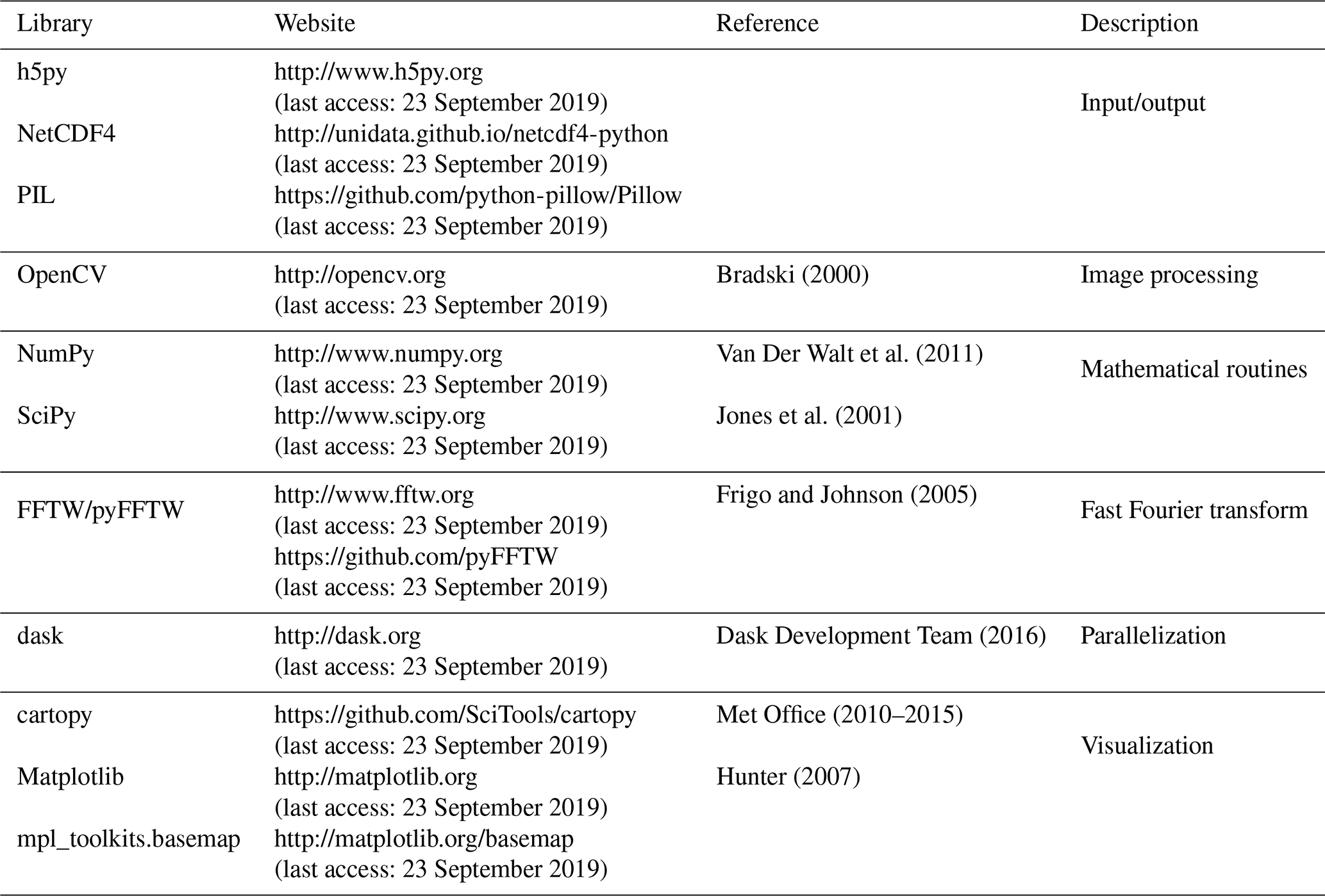
Pysteps development is done by using git, a distributed version control system. The source code of pysteps is hosted in GitHub (https://pysteps.github.io, last access: 23 September 2019). In addition to code hosting, the features of GitHub include development in multiple branches, issue tracking and wiki pages. Developers outside the core team may fork the main repository and integrate the proposed changes via pull requests, which allow community-driven development. Continuous integration and testing is done by using the Travis CI framework (https://travis-ci.com/pySTEPS/pysteps, last access: 23 September 2019).
Pysteps is published under the three-clause BSD license. It allows copying, redistribution and modification of the software as long as the modification are tracked and the source code is made available under the same license. The permissive license model makes the software easily accessible to potential users, even allowing use for commercial purposes.
3.2 External dependencies
Pysteps relies on several external libraries that are listed in Table 2. It is built on top of NumPy, SciPy and Matplotlib, that together provide a MATLAB-like computing environment in Python. These libraries provide data structures and wrappers for low-level BLAS and LAPACK libraries for high-performance matrix and array operations, image processing methods and also high-level functionality for data visualization. The NumPy array is the basic data structure used in pysteps.
Support for NetCDF (the default file format), HDF5 and various image file formats is implemented via the NetCDF4, h5py and PIL libraries. A complete list of supported input/output file formats is given in the official pysteps documentation. Plotting precipitation data with basemaps has been implemented via mpl_toolkits.basemap and cartopy packages. The Lucas–Kanade optical flow algorithm used in pysteps is implemented in the OpenCV library and accessed via a Python interface. Parallelized computation of nowcast ensembles is done by using Dask, which provides a platform-independent back end for low-level methods.
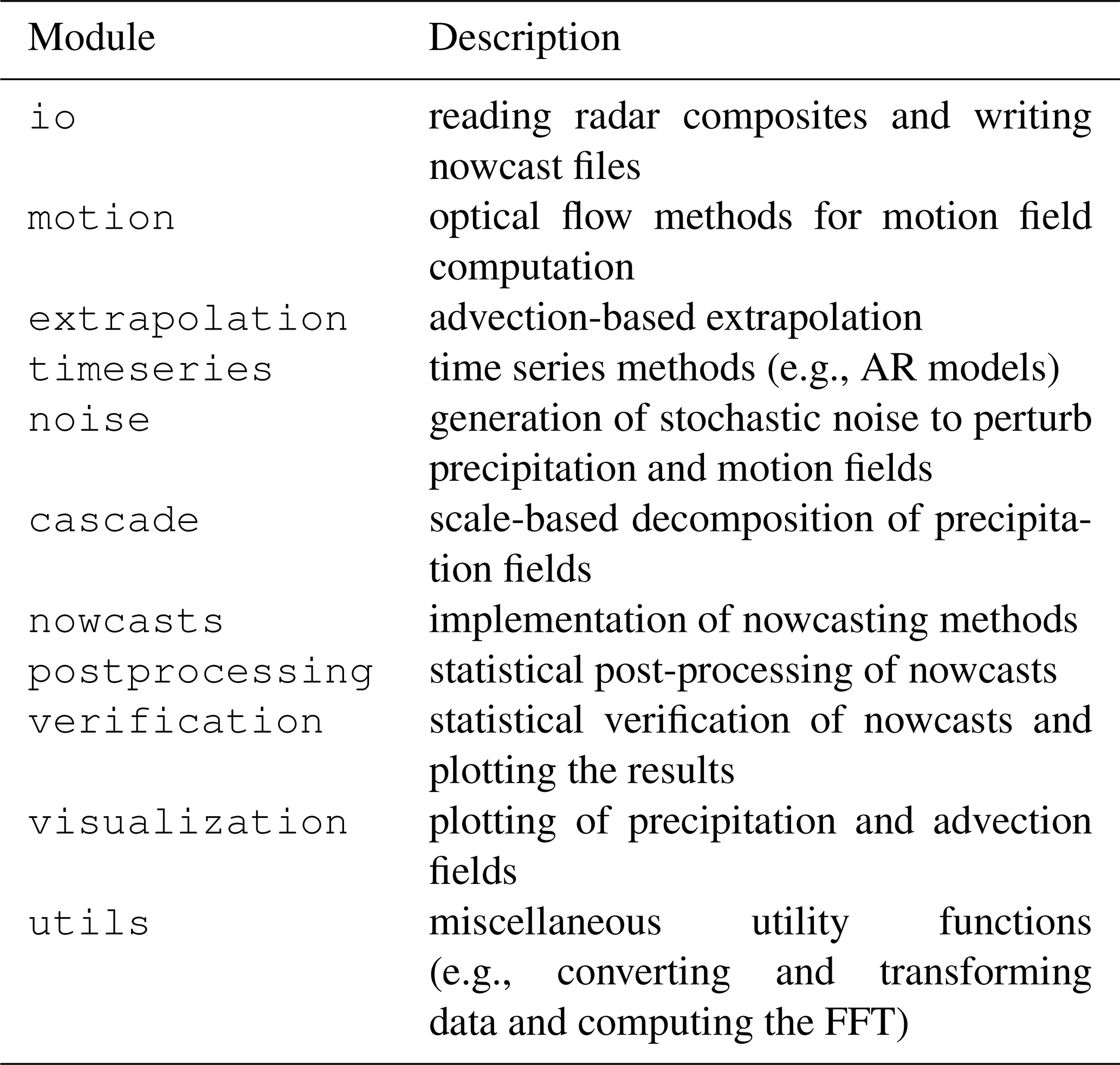
3.3 Key design principles
The aim of pysteps is to be a modular software library where all the main components are interchangeable. This makes the pysteps an ideal research platform for developing and testing new methods as well as a valuable tool for operational meteorology, easily allowing the comparison of different nowcast algorithms or running multi-model ensemble nowcasts. Pysteps is currently divided into 11 modules that perform different tasks. The modules and their descriptions are listed in Table 3.
The modularity is implemented via interface-based design. To this end, each module implements one subtask and an interface method for retrieving the desired method for this task. All mutually interchangeable methods implement the same interface. Another key principle is that whenever possible, the data are stored in n-dimensional arrays, which allow an efficient and compact representation.
The above design principles are demonstrated in the following example. A precipitation nowcast by using STEPS can be generated by
  >>> nowcast_method = nowcasts.get_method("steps")
  >>> nowcast = nowcast_method(R, V, num_timesteps)
where the required inputs are
-
R: array of shape () containing a time series of t observed precipitation intensity fields with shape (m,n),
-
V: a previously computed array of shape () containing the x and y components of the advection field
-
num_timesteps number of time steps to forecast.
Additional parameters can be specified by using keyword arguments. The output of stochastic nowcasting methods is a four-dimensional array of shape (num_ensemble_members, num_timesteps, height, width). For deterministic nowcasts, the first dimension is dropped.
3.4 Data structures
In addition to being modular, pysteps implements object-oriented features. However, instead of using customized classes, we use dictionaries and functions that operate on the dictionaries similarly to class member functions. This design decision is motivated by the principle of using the core Python data types rather than implementing customized classes. The flat design of pysteps should facilitate user interaction and embedding of individual modules and functions in other software. In this way, pysteps is similar to wradlib (Heistermann et al., 2013).
To demonstrate the above design, the following example shows how to construct a Gaussian bandpass filter for eight cascade levels using the filter_gaussian function implemented in the cascade.bandpass_filters module:
>>> filter = filter_gaussian(R.shape, 8)
The output is a dictionary with three elements: (1) one-dimensional weights corresponding to the radial wavenumbers, (2) a two-dimensional weight field for the FFT of the input image and (3) a list of central frequencies for each weight function (see Fig. 1). The resulting filter object can then be passed to decomposition_fft as follows:
>>> decomp = decomposition_fft(R, filter)
The decomposition is applied to a two-dimensional precipitation field R, and the output is again a dictionary with three-elements: (1) a three-dimensional array containing the eight cascade levels having the same dimension as R, (2) mean precipitation values of each cascade level and (3) standard deviations for each level. More detailed examples of pysteps usage are provided in Appendix A.
3.5 Workflow
Figure 4 illustrates the workflow for generating precipitation nowcasts using pysteps. The first step is reading the input data using the io module. Methods for reading radar composites from Australian Bureau of Meteorology (BoM), FMI, KNMI and MeteoSwiss have been implemented. In addition, the importers module supports reading the European-wide OPERA radar composites in the ODIM HDF5 format. Conversion from reflectivity (dBZ) to precipitation intensity (mm h−1) and other preprocessing can be done by using the utils module. Due to the modular design of pysteps, reading custom data formats and conversions (e.g., by using different Z−R relationships and polarimetric parameters) can also be implemented.
Reading the input data is followed by determination of the motion field using the methods implemented in the motion module. The precipitation intensity and motion fields are supplied as inputs to a user-chosen nowcasting method implemented in the nowcasts module. For the Lagrangian persistence method implemented in nowcasts.extrapolation, the remaining step of generating the nowcast is extrapolation.
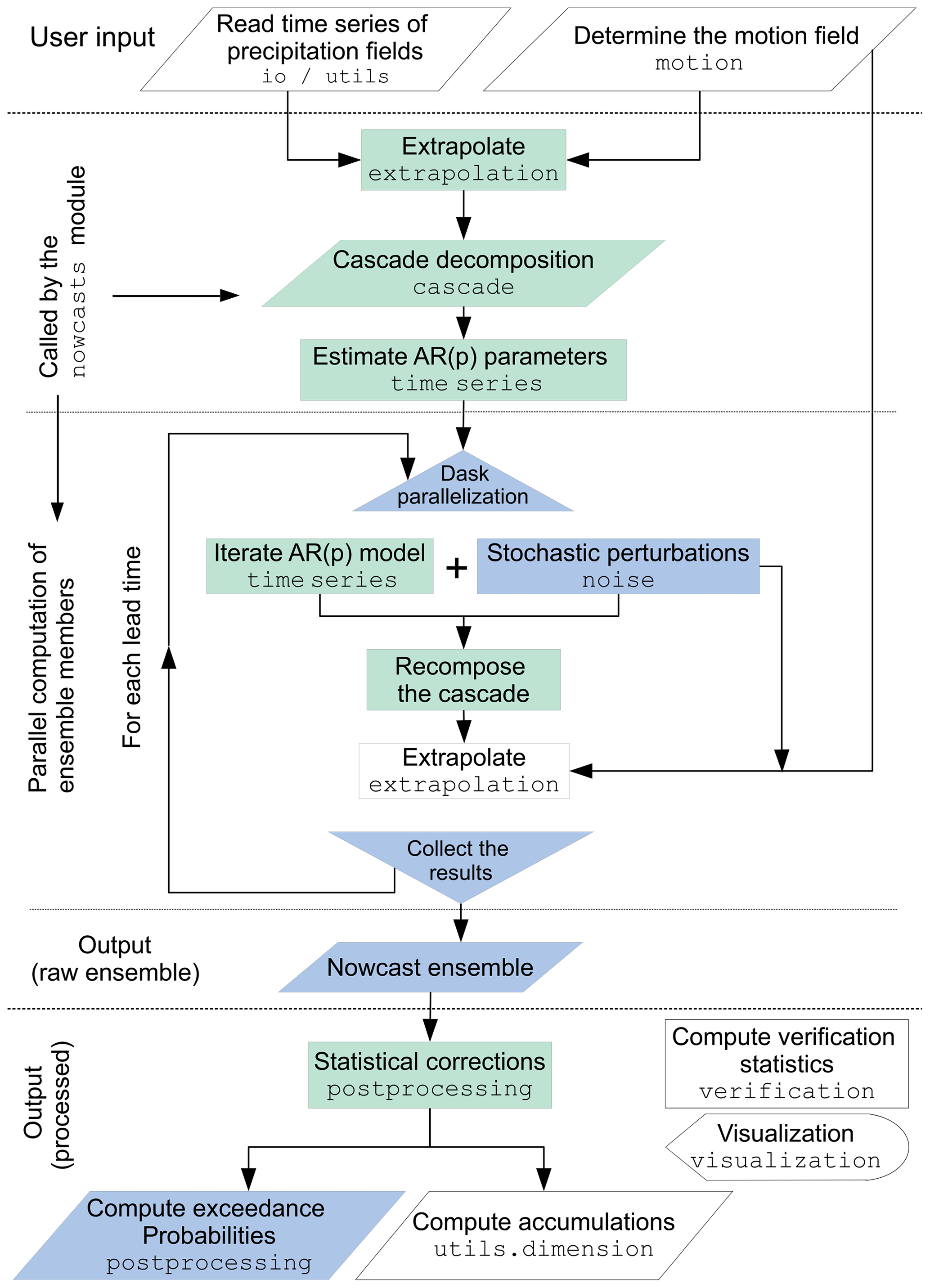
Figure 4Workflow for computing precipitation nowcasts using pysteps. For each chart element, the top row describes the task and the bottom row is the name of the module used for this purpose. White colors represent the operations that are done with all nowcasting methods. Green colors represent the additional operations included when the cascade decomposition and the autoregressive AR(p) model are applied (i.e., the S-PROG model). Finally, blue colors represent the operations that are done when stochastic perturbations are added and the ensemble computation is parallelized (i.e., the full STEPS model).
When the cascade decomposition and the autoregressive model are used for scale filtering (the S-PROG model), the additional steps include those marked with green color in Fig. 4. When generating ensembles (the STEPS model), stochastic perturbations are added to the AR(p) models and to the advection field using the methods implemented in the noise module. These steps are marked with blue color in Fig. 4.
The ensemble generation is parallelized by using the dask library. For each time step, this is done by splitting the computation to the available processor cores so that each core is responsible for computation of one ensemble member.
Given the input radar composites and the motion field, all operations involved in generating a nowcast are called from the nowcast module, except optional post-processing. This can be done either by supplying the requested method to the nowcast generator or separately by using the functionality implemented in the postprocessing module. The post-processing includes methods to ensure that the nowcasts have the same statistical properties of the observations (see Sect. 2.8), as well as methods for generating different products, such as ensemble mean or exceedance probabilities of given intensity thresholds. Computation of accumulations from instantaneous rain rates can be done by using the methods implemented in the utils.dimension module. Finally, the nowcasts or nowcast ensembles can be verified and plotted by using the verification and visualization modules, respectively.
Verification is an essential step of forecasting, not only to monitor forecast performance over time but also to provide feedback on how to improve the model itself (diagnostic verification). For an ensemble forecast, it is necessary to check whether it is unbiased and has the correct dispersion, and that the forecast probabilities are reliable and sharp (e.g., Jolliffe and Stephenson, 2003). In this section, we evaluate these attributes of pysteps ensemble nowcasts using radar composites from Switzerland and Finland, while data from the United States and Australia will also be used in Sects. 5 and 6.
4.1 Description of the data
As of 2019, the radar network operated by the FMI consists of 10 polarimetric C-band Doppler radars. After clutter filtering, the measured radar reflectivities are interpolated into a grid with spatial and temporal resolutions of 1 km and 5 min, respectively. The correction for the vertical profile of reflectivity (VPR) is applied in order to reduce range-dependent biases (Koistinen and Pohjola, 2014). Finally, reflectivities are converted to rainfall intensities using the Z−R relation, Z=223R1.53, adapted to the Finnish climate conditions (Leinonen et al., 2012). A total of 10 precipitation events from Finland containing both stratiform and convective precipitation were chosen for this study (Table 7).
Table 4Overview of the radar quantitative precipitation estimation (QPE) composites that have been used to evaluate pysteps. The grid size is given as the number of pixels in the x and y dimensions.
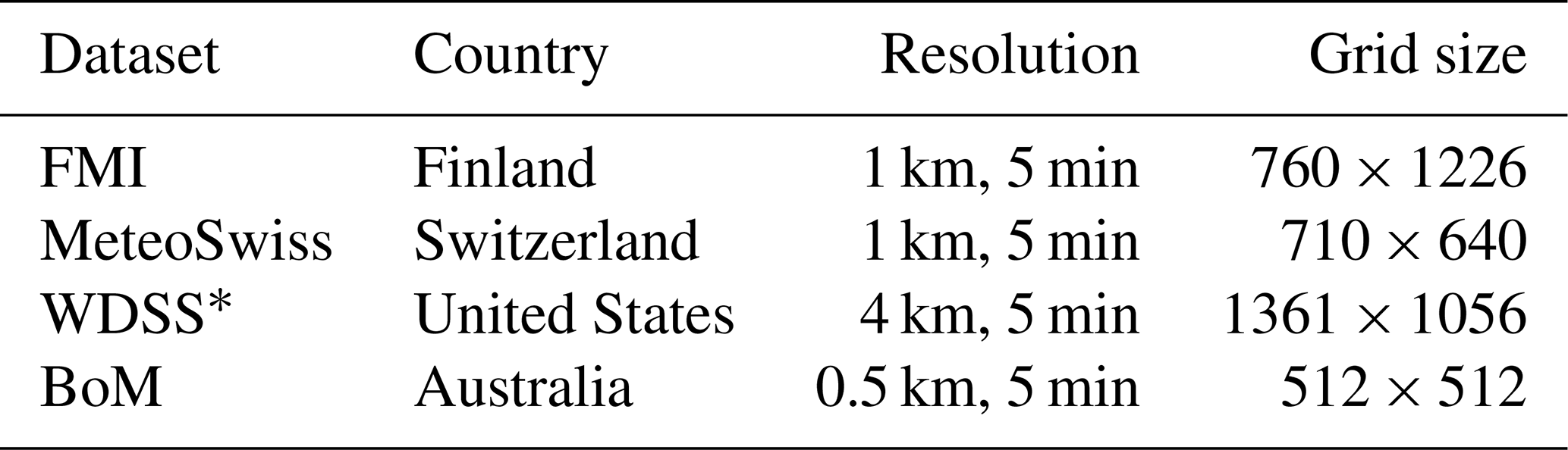
* Upscaled from original data at 1 km resolution (5445×4226).
The latest fourth-generation MeteoSwiss network consists of five polarimetric C-band Doppler radars (Germann et al., 2015). The quantitative precipitation estimation (QPE) product used in this study includes automatic hardware calibration, clutter filtering, correction for beam shielding, correction for VPR effects, Z−R relation (Z=316R1.5) and bias adjustment (Germann et al., 2006a). The radar composite is calculated on a 1 km grid every 5 min. Overall, 10 events consisting of predominantly convective precipitation were chosen from the Swiss data (Table 8).
The US dataset comprises the radar mosaics provided by Warning Decision Support System-Integrated Information (WDSS-II Lakshmanan et al., 2006, 2007), covering the continental United States at a spatial resolution of approximately 1 km. For the WDSS data, the resolution of the precipitation fields is upscaled from 1 to 4 km by averaging 4×4 grid points to reduce the computational requirements. The chosen precipitation events are described in Table 9.
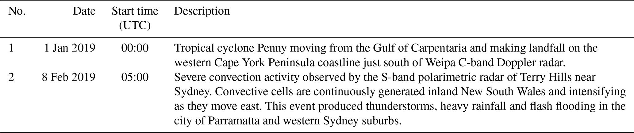
The radar network operated by BoM consists of 66 radars, mostly C-band Doppler radars, with S-band polarimetric Doppler radars operating at four major cities. Raw reflectivity observations are quality controlled in real time to remove non-meteorological echoes and estimate the reflectivity at the Earth's surface. This equivalent reflectivity at the surface is converted into an instantaneous rainfall rate by use of power–law functions tuned on a per radar basis. Finally, rainfall depths are estimated by adjusting the bias of instantaneous rainfall rates based on observations at real-time gauge locations. The QPE grids are calculated with a spatial resolution of 0.5 km every 5 min. The BoM radar dataset comprises two precipitation events: a tropical cyclone in northern Australia and a severe convective event in Sydney (Table 10).
Table 4 summarizes the different data sources and resolutions.
4.2 Verification metrics
Pysteps includes a number of verification metrics to help users to analyze the general characteristics of the nowcasts in terms of consistency and quality (or goodness). Probabilistic forecasts have been verified using the relative operating characteristic (ROC) curve, reliability diagrams and rank histograms, as implemented in the verification module of pysteps.
The ROC curve (Jolliffe and Stephenson, 2003) measures the ability of a probabilistic forecast to discriminate between precipitation and no precipitation exceeding a given intensity threshold. For a set of probability thresholds, the ROC curve is constructed by plotting the probability of detection (POD) against the false alarm rate (POFD), not to be confused with the false alarm ratio (FAR). For a perfect forecast, the curve passes through the upper left corner (i.e., 100 % hit rate and 0 % false alarm rate). The area under the ROC curve can be used as a measure of potential skill. For more details on the contingency tables and the formulas of the categorical scores, the reader is referred to Jolliffe and Stephenson (2003).
The reliability diagram (Bröcker and Smith, 2007) measures the bias (reliability) and resolution of a probabilistic forecast. For a given intensity threshold, the diagram shows the forecast probability against the observed frequencies, where the probability range [0,1] is divided into n bins. For a perfectly reliable forecast, the curve lies on the diagonal. The reliability diagram is often accompanied by a histogram showing the sample size in each bin (sharpness diagram). A sharp forecast has few samples in the middle of the histogram and many on the sides (probability of either 1 or 0).
The rank histogram (Hamill, 2001) measures how well the ensemble spread corresponds to the observed uncertainty. For each nowcast grid pixel, the ensemble members are ranked in increasing order. A pooled histogram is computed by assigning each verifying observation a bin which it falls into among the ensemble members. The first and last bins are assigned for observations below or above all members, respectively. For a forecast ensemble whose distribution is consistent with the observations, the histogram is flat and no observations fall into the first or last bin. To handle ties (e.g., when both the observed precipitation and several ensemble members are equal to 0), we implemented the method of Hamill and Colucci (1997). The method randomly chooses a bin between (M+1) and , where M is the number of members smaller than the observation and Mtied is the number of ties (ensemble members equal to the observation).
An additional metric that can be derived from rank histograms is the outlier percentage (OP). The OP measures the proportion of observations falling outside the ensemble, defined by
where hi denotes the ith bin of the rank histogram.
Pysteps also includes standard neighborhood verification methods, such as the fractions skill score (FSS). FSS provides an intuitive assessment of the dependency of skill on spatial scale from high-resolution precipitation forecasts (Mittermaier and Roberts, 2010). The FSS is computed by comparing the forecast and observed fractional coverage of precipitation exceeding certain thresholds in spatial windows (neighborhoods) of increasing size. Using FSS it is possible to determine how the forecast skill varies with neighborhood size and then determine the smallest scale that provides a sufficiently skillful forecast.
4.3 Verification results
The quality of ensemble nowcasts produced by pysteps was verified by using the MeteoSwiss data and the default configuration listed in Table 5. Using the reliability diagram, ROC curve and rank histogram as verification metrics, the results of the experiments are shown in Figs. 5–7. The results obtained by using the FMI data were very similar and thus not shown here.
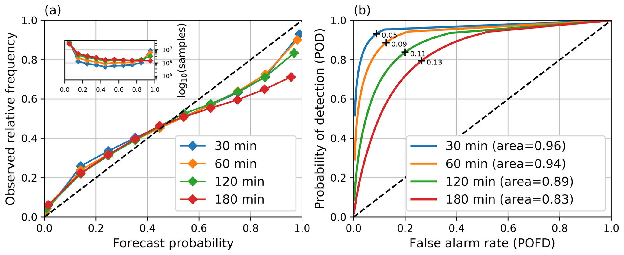
Figure 5Reliability diagrams (a) and ROC curves (b) computed from STEPS nowcasts during the MeteoSwiss events listed in Table 8 with different lead times and threshold 0.1 mm h−1. The default settings listed in Table 5 were used for computing the nowcasts. The optimal probability thresholds that maximize POD-POFD are marked in the ROC curves with black crosses.
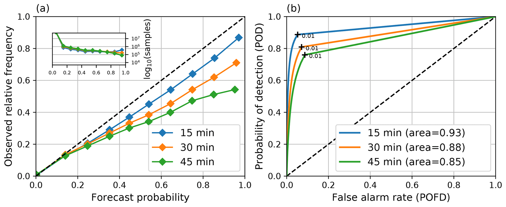
Figure 5 shows that for the 0.1 mm h−1 intensity threshold, reliable and sharp nowcasts can be obtained up to 2 h. The ROC area remains over 0.85, and the deviation of the reliability diagrams from the diagonal remains below 0.25. However, there is a noticeable loss of sharpness after 3 h. In addition, the curved shape of the reliability diagrams indicates that the pysteps nowcasts are slightly overconfident (Tippett et al., 2014).
When a higher 5 mm h−1 intensity threshold is used, Fig. 6a shows a significant deviation of the reliability diagram from the diagonal only after 45 min, which is accompanied by loss of sharpness. However, the ROC area remains above 0.8, indicating potentially useful skill. This suggests that more reliable nowcasts could be obtained by implementing additional calibration procedures in a future version of pysteps. Another observation that suggests lack of calibration is that the optimal nowcasts for precipitation/no precipitation are obtained by choosing a very low probability threshold (for a well-calibrated nowcast, this would be 0.5).
The rank histograms (Fig. 7) also show some ensemble underdispersion with larger values on the first and last bins. In general, we found that there are more misses than false alarms (i.e., cases when all members are lower than the observations). This occurs, for instance, in cases of convective initiation. Despite the ability of pysteps to generate some new light random rain, it is not designed to represent the uncertainty related to an explosive initiation of a thunderstorm.
4.4 Numerical diffusion analysis
Conventional semi-Lagrangian schemes are implemented in a recursive way so that the precipitation intensities are interpolated at each time step, which usually leads to substantial numerical diffusion (i.e., loss of power at high spatial frequencies). In the pysteps method (the extrapolation.semilagrangian module), this is done by iteratively tracing the locations of precipitation parcels and interpolating the intensities only as the final step of the advection (Germann and Zawadzki, 2002).
To verify the advantage of this implementation, we computed radially averaged Fourier spectra of deterministic nowcasts at various lead times for FMI event no. 3 (Fig. 8). The analysis is performed using the three optical flow methods to understand whether the semi-Lagrangian scheme is sensitive to quality of the motion field. Figure 8 shows an almost perfect overlap of the forecast and observed spectra, an indication that the numerical diffusion of the semi-Lagrangian scheme is very low. Several cases have been analyzed and provided similar results (not shown).
4.5 Spatial structure analysis
The aim of probabilistic nowcasting is to generate a reliable ensemble of equiprobable realizations of precipitation fields characterized by power spectra similar to those in Fig. 8. Figure 9a shows the average spectra of a stochastic 48-member nowcast for FMI precipitation event no. 3. Despite a small loss of power for scales (<100 km), all spectra are close to the observations. In other words, the spatial structure of ensemble members remains realistic at all forecast lead times.
Figure 9b shows the results of the same analysis but for the ensemble mean forecast (the average of ensemble members). The process of ensemble averaging should produce precipitation fields that become smoother with lead time, which is the aftermath of the loss of predictability at small scales (Surcel et al., 2014). As expected, Fig. 9b shows a gradual loss of power at small scales. The departure of the forecast spectra from the observed ones occurs at increasing wavelengths, i.e., ≈16 km at 5 min and ≈128 km at 60 min. However, after 30 min, there is a certain increase of power at wavelengths smaller than 16–32 km. This behavior is attributed to the limited ensemble size, which is not large enough to filter out precipitation features at small scales. Thus, one may argue that if the ensemble is too small to model the loss of predictability at such scales, it may also be too small to reliably model the forecast uncertainty.
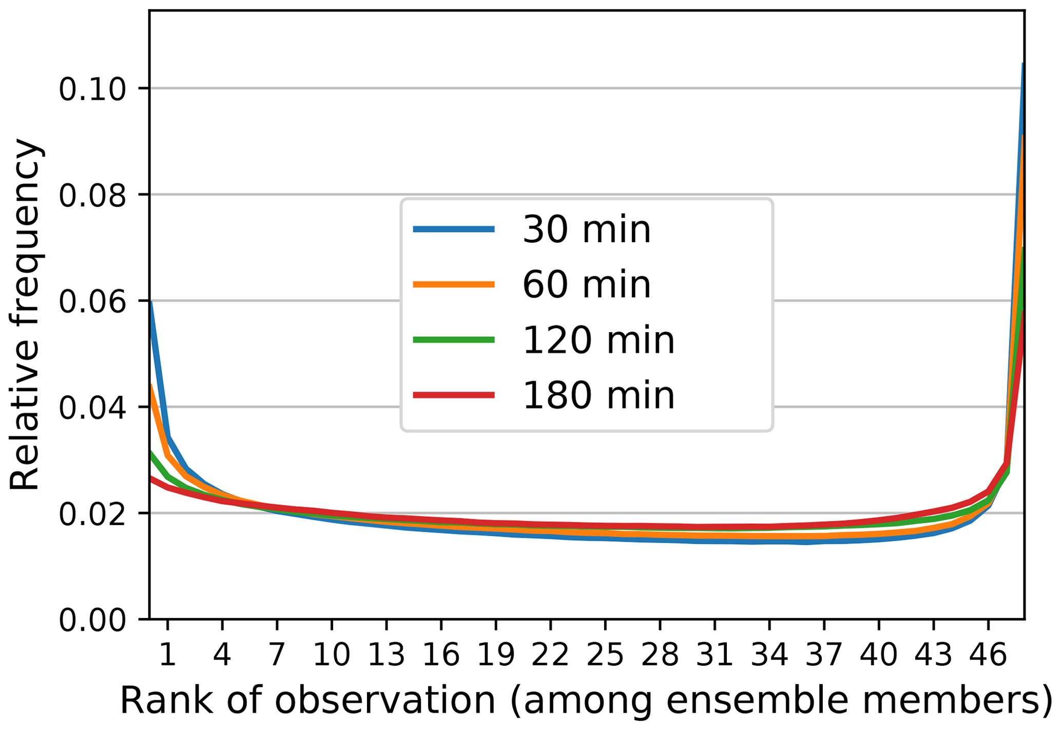
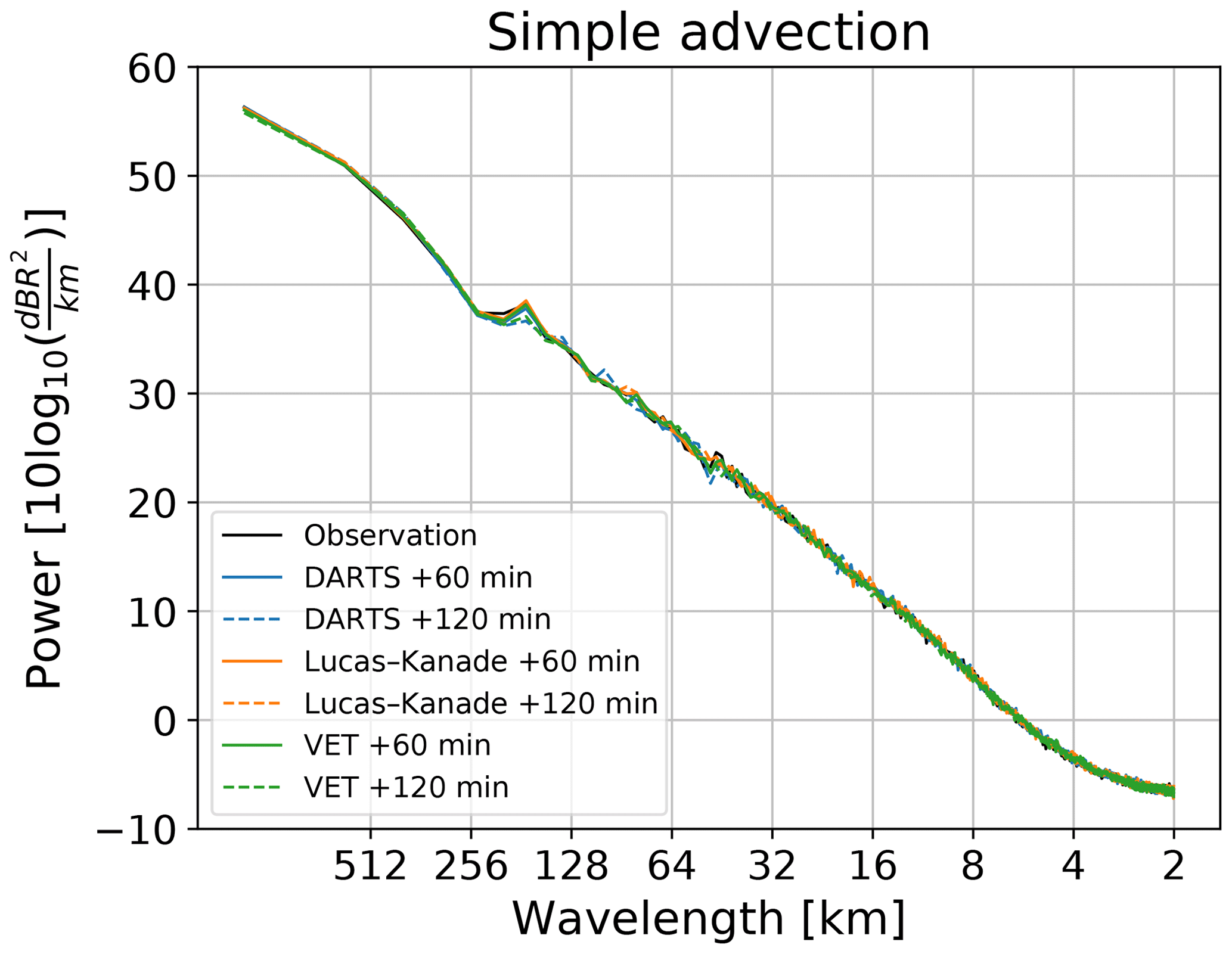
Figure 8Numerical diffusion analysis of the semi-Lagrangian advection scheme using radially averaged Fourier spectra for different optical flow methods and different forecast lead times. The nowcasts are for FMI event no. 3 (16:00 UTC on 28 September 2016).
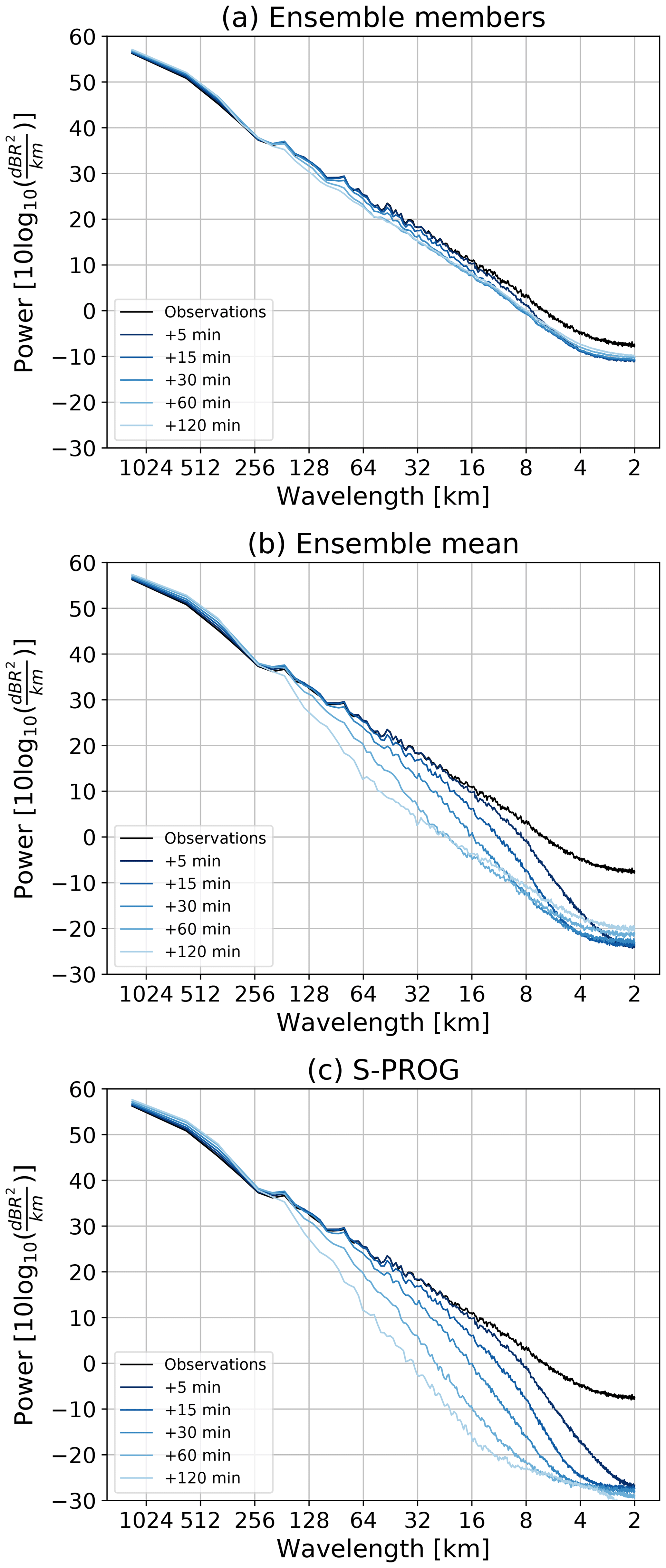
Figure 9Spatial structure analysis of (a) stochastic ensemble members, (b) ensemble mean and (c) S-PROG filtering. To be comparable, the incremental mask and probability matching were used for both the ensemble mean and S-PROG nowcasts. All nowcasts used the Lucas–Kanade optical flow on the same event of Fig. 8. The ensemble is composed of 48 members. All models used a cascade of eight levels without motion perturbations.
An alternative way to deterministically represent the forecast uncertainty is to filter out the unpredictable features using the S-PROG model (Fig. 9c). Also, in this case, the departures of forecast spectra from the observed one occur gradually as in the ensemble mean. The first two lead times are remarkably similar, while for lead times beyond 30 min the S-PROG filtering is stronger (at small spatial wavelengths). Again, this level of filtering could be reached with an ensemble of infinite size.
The previous result suggests that we could exploit the discrepancies between the S-PROG and ensemble mean spectra to obtain an estimate of the required ensemble size (as a function of spatial scale and lead time). If the two spectra are similar, it is an indication that the ensemble is large enough.
4.6 Temporal structure analysis
To demonstrate the effectiveness of the hierarchy of AR(2) models in modeling the temporal evolution of precipitation, we derived the theoretical ACF from the estimated AR parameters (see Eq. 7). The obtained ACF is compared to the empirical ACF between the nowcasts and the corresponding observations. The correlation coefficients are computed separately for each cascade level obtained using the bandpass filters shown in Fig. 1.
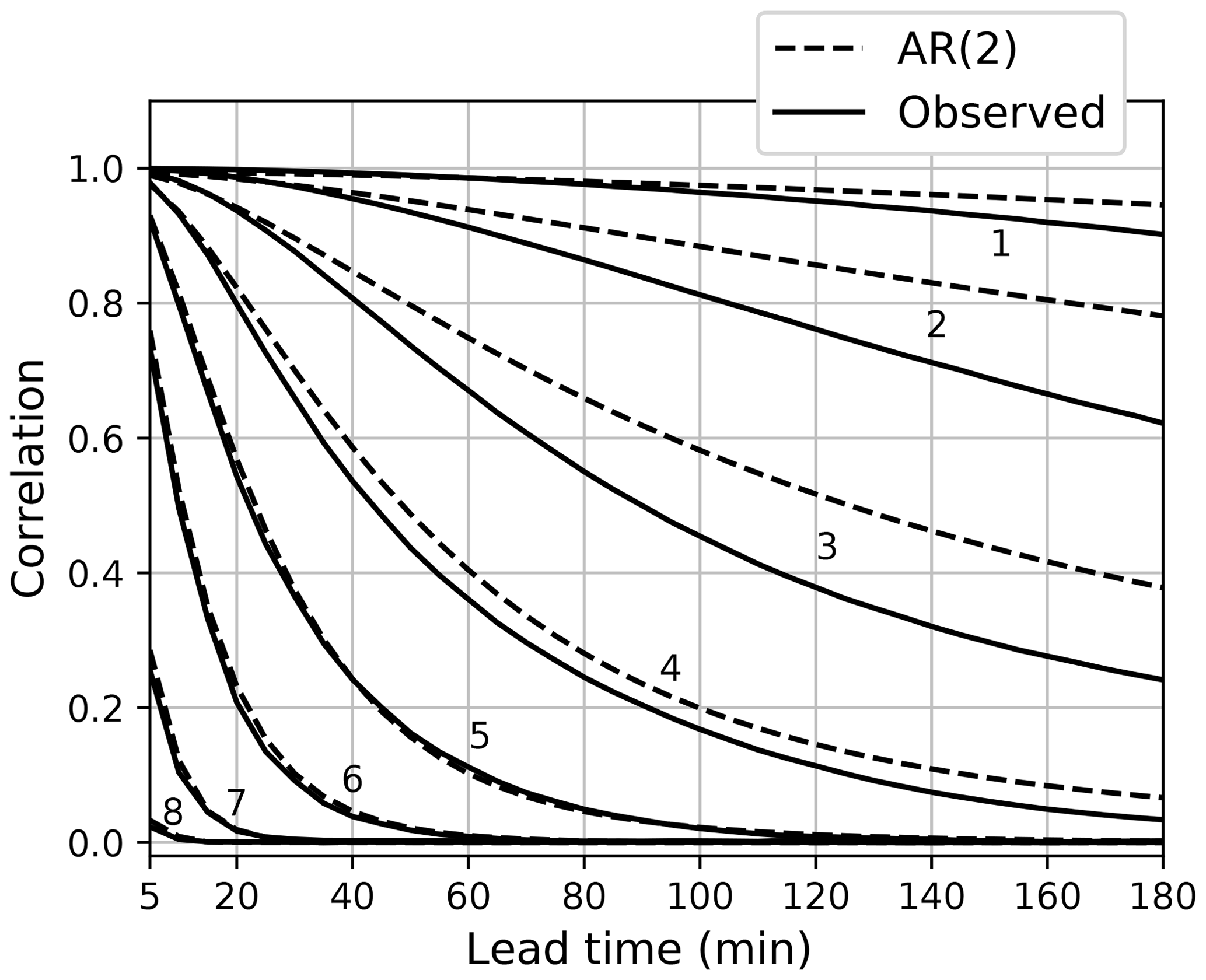
Figure 10Temporal auto-correlation estimates obtained from AR(2) models (dashed lines) and the correlation between an extrapolation nowcast and the corresponding observations. The analysis is based on the FMI events (Table 7). The line numbers correspond to the frequency bands shown in Fig. 1 from left to right.
Figure 10 shows the average theoretical and empirical ACFs for all the FMI cases. It clearly indicates that the AR(2) process gives accurate estimates of the temporal auto-correlations up to 3 h. For smaller scales (0–35 km) having short lifetimes, the estimates coincide nearly exactly with the observed ones, but for larger scales the auto-correlations are slightly overestimated. This is due to the relatively short memory of the AR(2) process compared to the precipitation lifetimes at these scales (over 2 h).
The objective of this section is to analyze the sensitivity of pysteps to its configuration options and parameters such as the optical flow method, the ensemble size, the parameter localization and the cascade decomposition. The default pysteps configuration used in Sect. 4 is based on the results presented here.
5.1 Optical flow and scale filtering
Determination of the advection field by optical flow is a key component of any extrapolation-based nowcasting system. Pysteps allows to easily analyze the impact of the optical flow method and also scale filtering on the forecast skill. Moreover, the three methods currently available in the motion module constitute an ideal testbed as they cover three very distinct approaches; see the references in Sect. 2.1 for details. The experiments were done by using the MeteoSwiss and US precipitation events described in Tables 8 and 9.
Each optical flow method was used with two deterministic nowcasting methods: a simple extrapolation-based method and S-PROG, which incorporates a scale filtering procedure as described in Seed (2003). Both methods are available in the nowcasts.extrapolation and nowcasts.sprog modules, respectively. The VET and Lucas–Kanade methods use two input images, while DARTS uses nine input images. The forecast quality was evaluated using the critical success index (CSI) and the mean absolute error (MAE) as described in Jolliffe and Stephenson (2003).
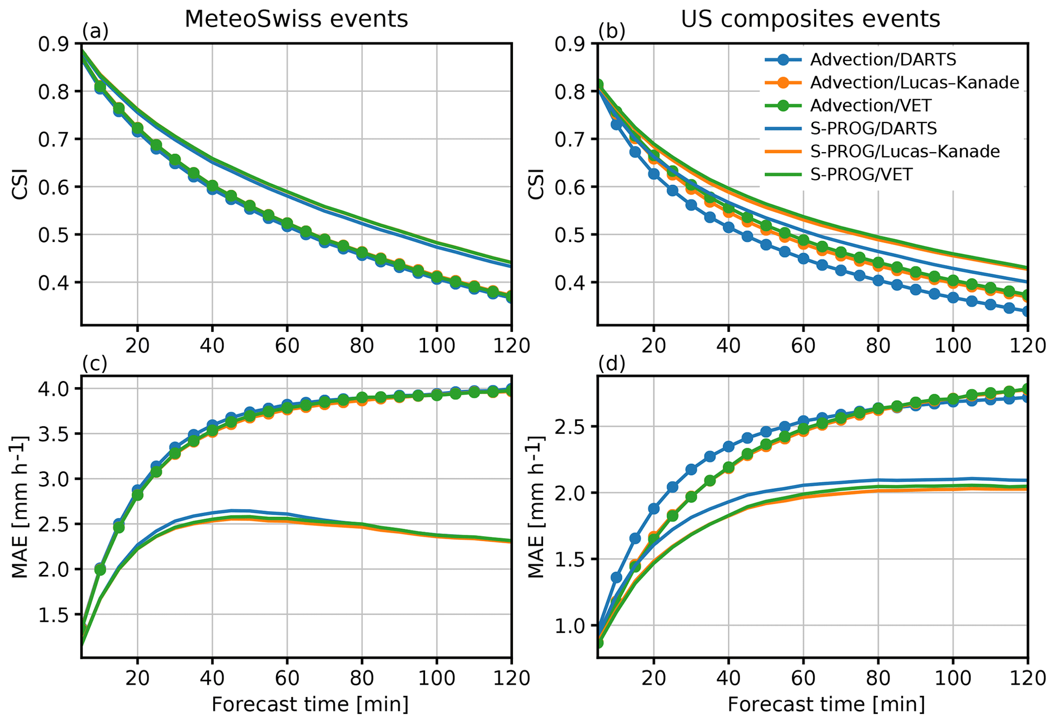
Figure 11Comparison of forecast skill using different optical flow and extrapolation methods. Panels (a) and (c) show the averaged CSI and MAE for the MeteoSwiss events listed in Table 8, while (b) and (d) show the same results but for the US events listed in Table 9. The CSI is computed using a 0.1 mm h−1 threshold.
The results of the experiments are shown in Fig. 11. First of all, large differences between the simple extrapolation and S-PROG nowcasts are observed, which is mainly due to the scale filtering implemented in S-PROG (see Sect. 4.5). For the MeteoSwiss events, applying the filtering improves both CSI and MAE, especially at longer lead times (Fig. 11a and c). After 2 h, the S-PROG nowcasts show a ∼20 % increase in the CSI and ∼40 % reduction in the MAE. A similar behavior is observed for the US events (Fig. 11b and 11d) but with a ∼20 % the reduction in MAE after 2 h.
On the other hand, no significant differences can be observed between different optical flow methods (less than 2 %), with DARTS performing slightly worse than the other methods. This is possibly explained by the fact that, with the default configuration, DARTS produces only a large-scale approximation of the advection field.
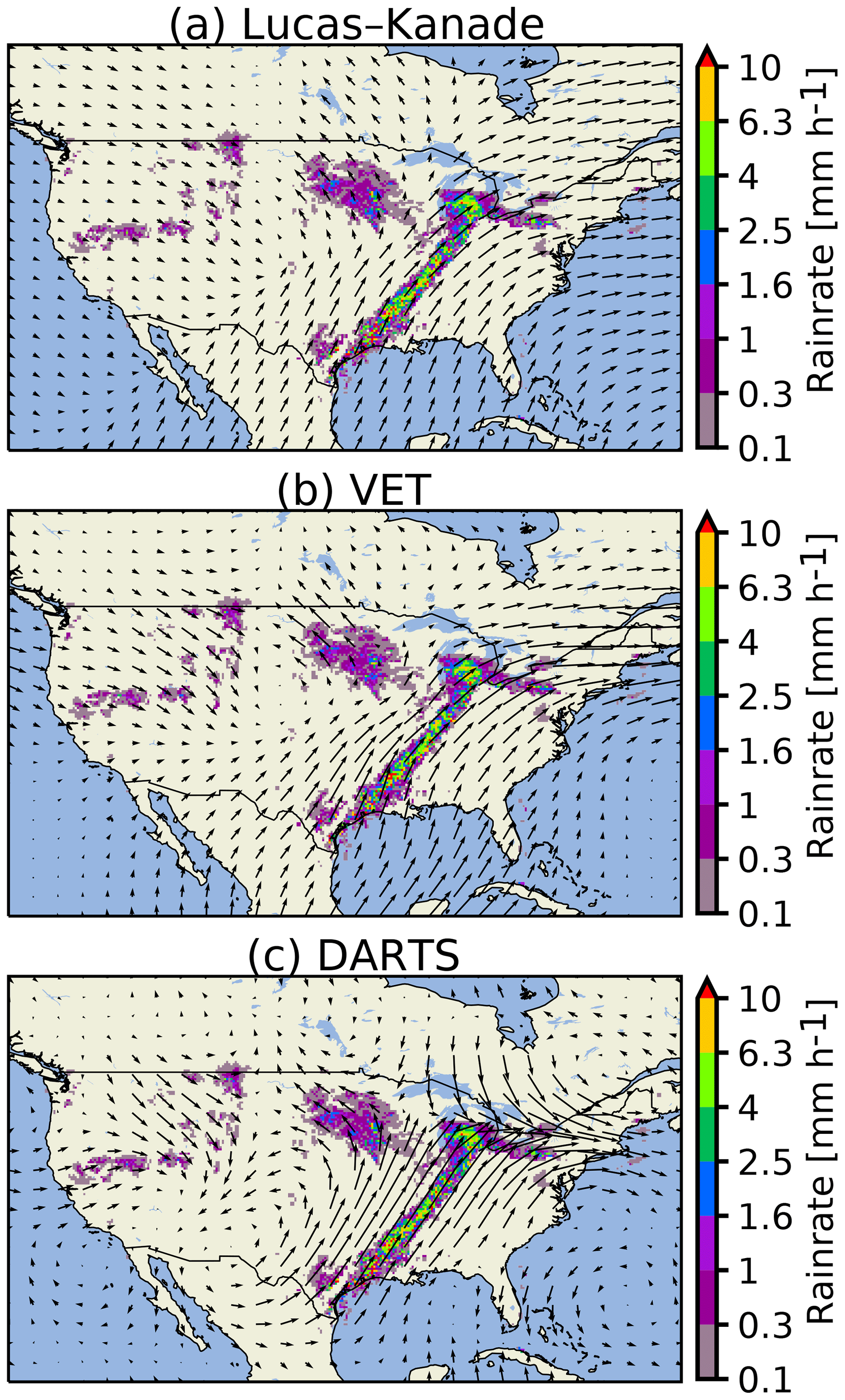
Figure 12Comparison of advection fields obtained by different optical flow methods for a selected precipitation event: US, 11 April 2013 at 08:00 UTC.
Figure 12 shows advection fields obtained using different optical flow methods for a selected case (US, 11 April 2013 at 08:00 UTC). Lucas–Kanade and VET produce smooth fields that are remarkably similar, particularly close to the precipitation areas (Fig. 12a and b). Within precipitation areas, DARTS produces similar motion fields to the other two methods, but outside precipitation the fields are considerably different.
Table 6Average computation times of different optical flow methods in the MeteoSwiss and FMI domains (seconds). Domain sizes are given in parentheses.

We also measured the computation times of different optical flow methods in the MeteoSwiss and FMI domains, and the results are shown in Table 6. The experiments were done using an Intel Xeon E5645 CPU with 12 cores running at 2.4 GHz with parallelization enabled in the optical flow methods. The results reflect the fact that the Fourier space and local methods (DARTS and Lucas–Kanade) have significantly lower computational requirements than variational methods (VET), which are however still within the needs of a real-time operational system. Thus, our conclusion from the results shown in Fig. 11 and Table 6 is that the choice of the optical flow method plays a less significant role, while nowcast errors are more clearly determined by the dynamic scaling properties of precipitation as highlighted by the large impact of scale filtering on the forecast skill.
5.2 Ensemble size
The ensemble size is one of the main factors contributing to the quality and computation time of pysteps nowcasts, and one has to make a trade-off between these two. To determine the optimal number, the skill of the nowcasts with different intensity thresholds and ensemble sizes was evaluated by using two metrics. These are the area under the ROC curve and the outlier percentage (OP). The results are shown in Figs. 13 and 14.

Figure 13ROC areas for (a) 0.1 mm h−1 and (b) 5 mm h−1 thresholds with different ensemble sizes as a function of lead time during the MeteoSwiss events listed in Table 8.
Figure 13 shows that the choice of the ensemble size plays a significant role, which is particularly true when nowcasts of higher precipitation intensities are desired. Figure 13a shows that for n=6, the ROC area falls below 0.85 after 2 h, while it is close to 0.9 when n is increased to 48. However, there is only marginal improvement when n is increased from 24 to 48, which suggests that 24 members are sufficient when nowcasts of precipitation/no precipitation are desired with low-intensity thresholds (e.g., 0.1 mm h−1). On the other hand, Fig. 13b shows that when the threshold is increased to 5 mm h−1, a significant improvement can be expected when increasing n from 48 to 96 or even over 100.
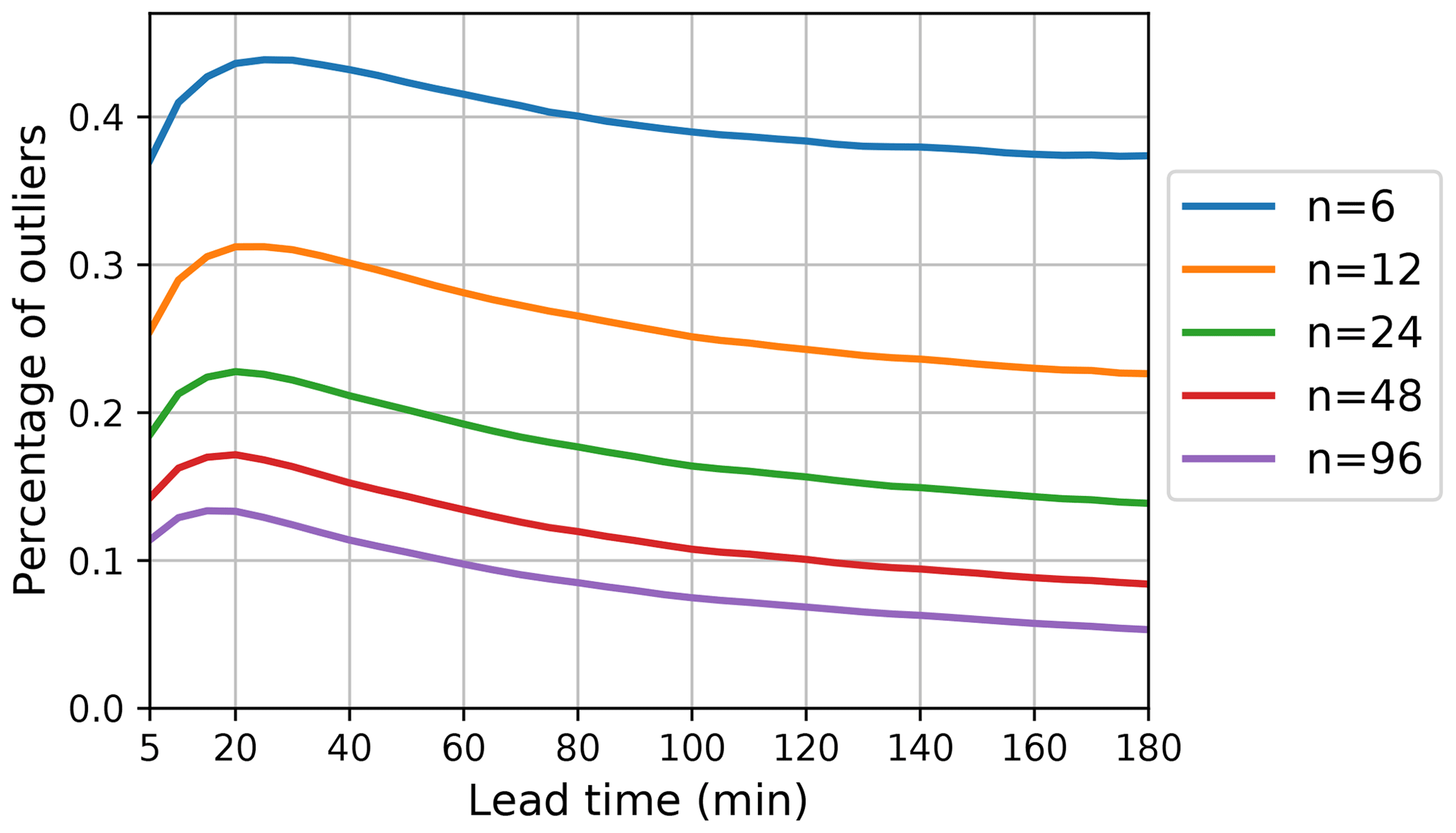
Figure 14Outlier percentages (OPs) with different ensemble sizes as a function of lead time during the MeteoSwiss events listed in Table 8.
The OP is highly dependent on the ensemble size, which can be observed from Fig. 14. With 96 ensemble members, OP is below 15 % after 20 min, which indicates that the ensembles are well able to capture the uncertainties in the spatiotemporal evolution of precipitation. The OP could be further reduced by increasing the ensemble size over 100. Another observation from Fig. 14 is the significant dependence of OP on the lead time. The highest OP can be observed at 20 min, and after 3 h it is up to 50 % smaller.
We also analyzed the computation times needed to generate nowcast ensembles. In a real-time setting, it is essential to know how many ensemble members can be produced before the arrival of the next input radar rainfall image (usually every 5 min). To this end, 1 h nowcasts were computed with different ensemble sizes and number of parallel threads using the FMI and MeteoSwiss data listed in Tables 7 and 8, respectively.
The results of the above experiments are shown in Fig. 15. Figure 15a shows that for the input grid of 710×640 pixels used in the MeteoSwiss domain, it is possible to generate 1 h nowcast ensembles of up to 48 members in less than 2 min using a server with 12 processor cores.
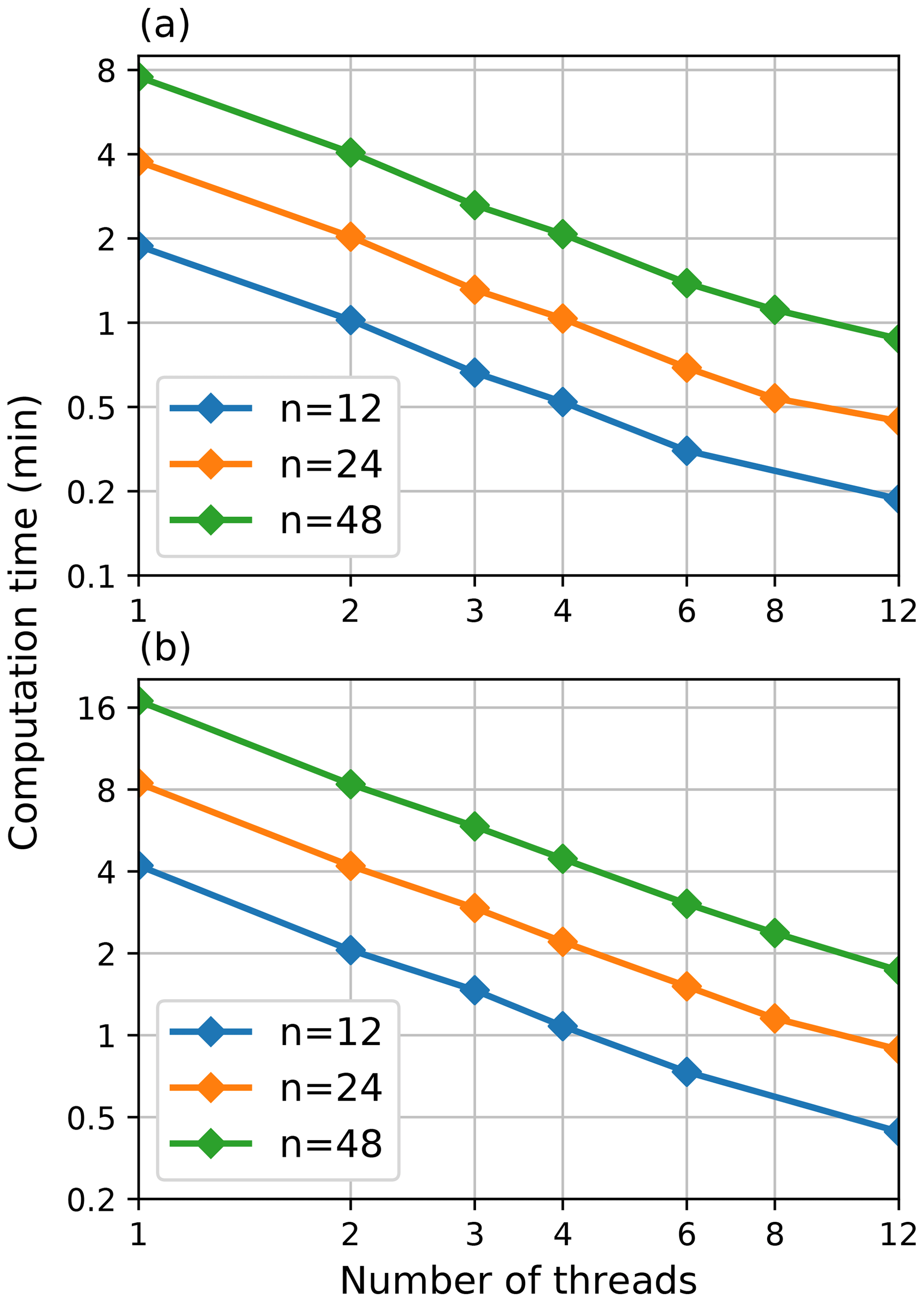
Figure 15Averaged computation times of pysteps nowcast ensembles with different ensemble sizes and number of parallel threads for the (a) MeteoSwiss and (b) FMI domain. The grid sizes for the domains are 710×640 and 760×1226 pixels, respectively. The 1 h nowcasts with 12 time steps of 5 min were computed for both domains. The computation times include only the ensemble computation, excluding the optical flow, the initialization of the model and writing the results to disk.
The results for the larger FMI domain with grid size of 760×1226 pixels are shown in Fig. 15b. Compared to the MeteoSwiss domain, the height of the grid is doubled, which also doubles the computation time (the computational complexity increases quadratically with respect to grid size). Nevertheless, using 12 processor cores, the computation time of a 48-member ensemble still remains below 2 min.
In addition, Fig. 15a and b show the effectiveness of the parallelization scheme implemented in pysteps. That is, when plotted in logarithmic scale, the computation time decreases approximately linearly with respect to the number of threads (i.e., the computation time is halved when the number of threads is multiplied by 2).
5.3 Localization
This experiment investigates the impact of localization on the nowcast quality. In this context, localization means restricting the nowcasting model into small subdomains instead of applying it the whole domain assuming spatial homogeneity of the precipitation field, as in the earlier STEPS implementations (e.g., Bowler et al., 2006). To this end, the short-space approach presented in Nerini et al. (2017) for stochastic noise generation is generalized to the whole nowcasting system (see module nowcasts.sseps). Adapting the approach described in Sideris et al. (2018), the parameter estimation and the nowcasting model are implemented in a moving window of predetermined size. The localization is applied to the cascade decomposition, the autoregressive process (5), the non-parametric Fourier filter (10) and the probability matching (15).
The impact of localization is assessed in terms of rank histograms and reliability diagrams (threshold of 1.0 mm h−1) for a 30 min lead time (Fig. 16). The localization shows positive effects in the ensemble spread, which improves both in terms of reliability and conditional bias, although we also observe a slight decrease of sharpness. This is reflected in the rank histograms, which tend to get flatter as the localization window gets smaller. This seems to be mainly driven by a reduction in the proportion of observations lying above the ensemble, which reduces from approximately 13 % to 8 %.
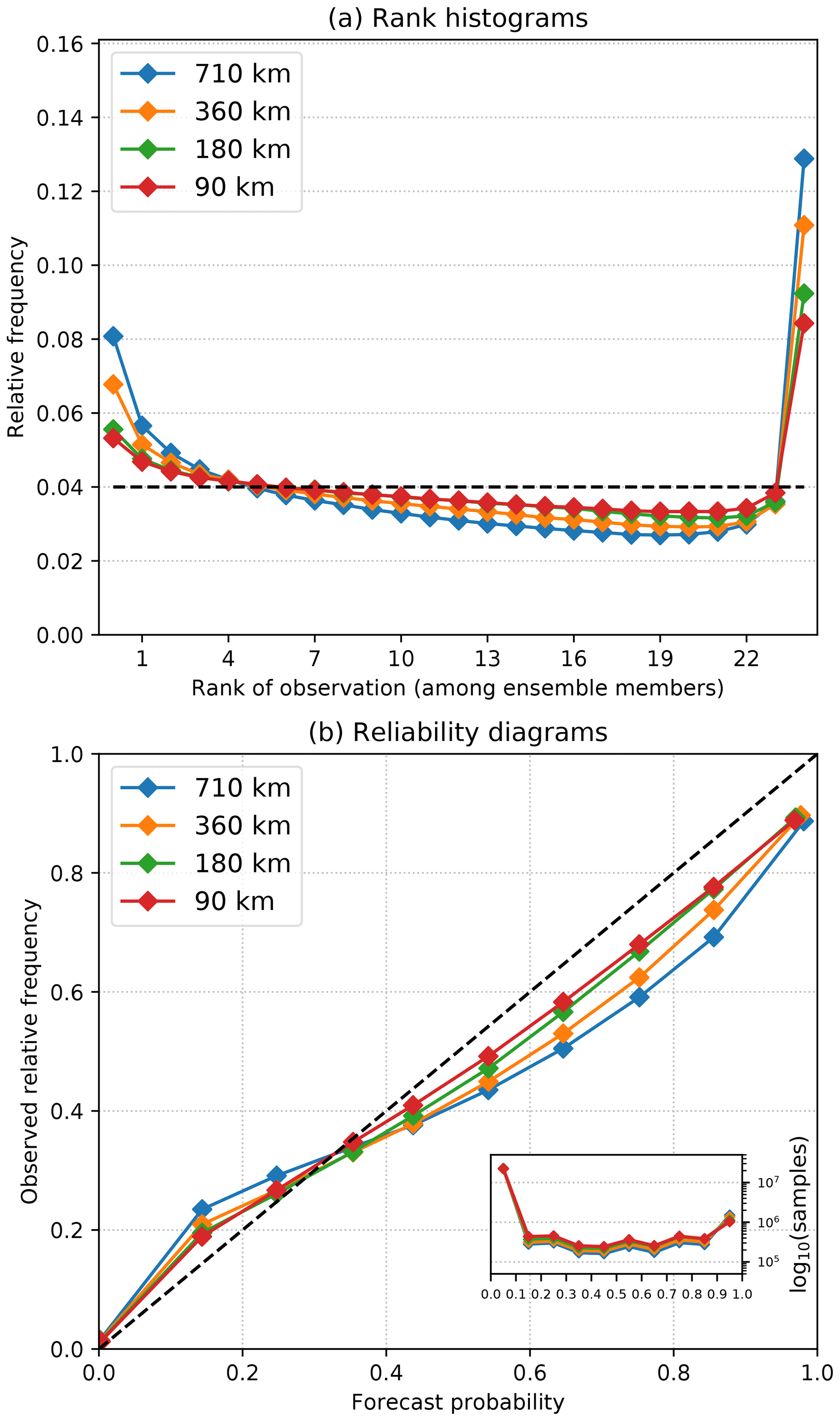
Figure 16Effect of localization in terms of (a) rank histograms and (b) reliability diagrams computed for the 30 min lead time and 1 mm h−1 during the MeteoSwiss events (Table 8). The localization window was reduced from the full domain (710 km) to three different local scales (360, 180 and 90 km).
5.4 Cascade decomposition
The cascade decomposition was designed to account for dynamic scaling (i.e., the dependence of predictability on spatial scale; see Sect. 2.4). Without the decomposition, precipitation fields are expected to evolve similarly at all spatial scales following a single AR process. In such cases, the lifetime of small-scale (large-scale) precipitation features would be overestimated (underestimated). Thus, our main hypothesis is that dynamic scaling properties are necessary to produce a realistic temporal evolution (lifetime) of precipitation across spatial scales. Consequently, this would give correct ensemble dispersion because the standard deviation of the perturbations is inversely related to predictability via Eq. (6).
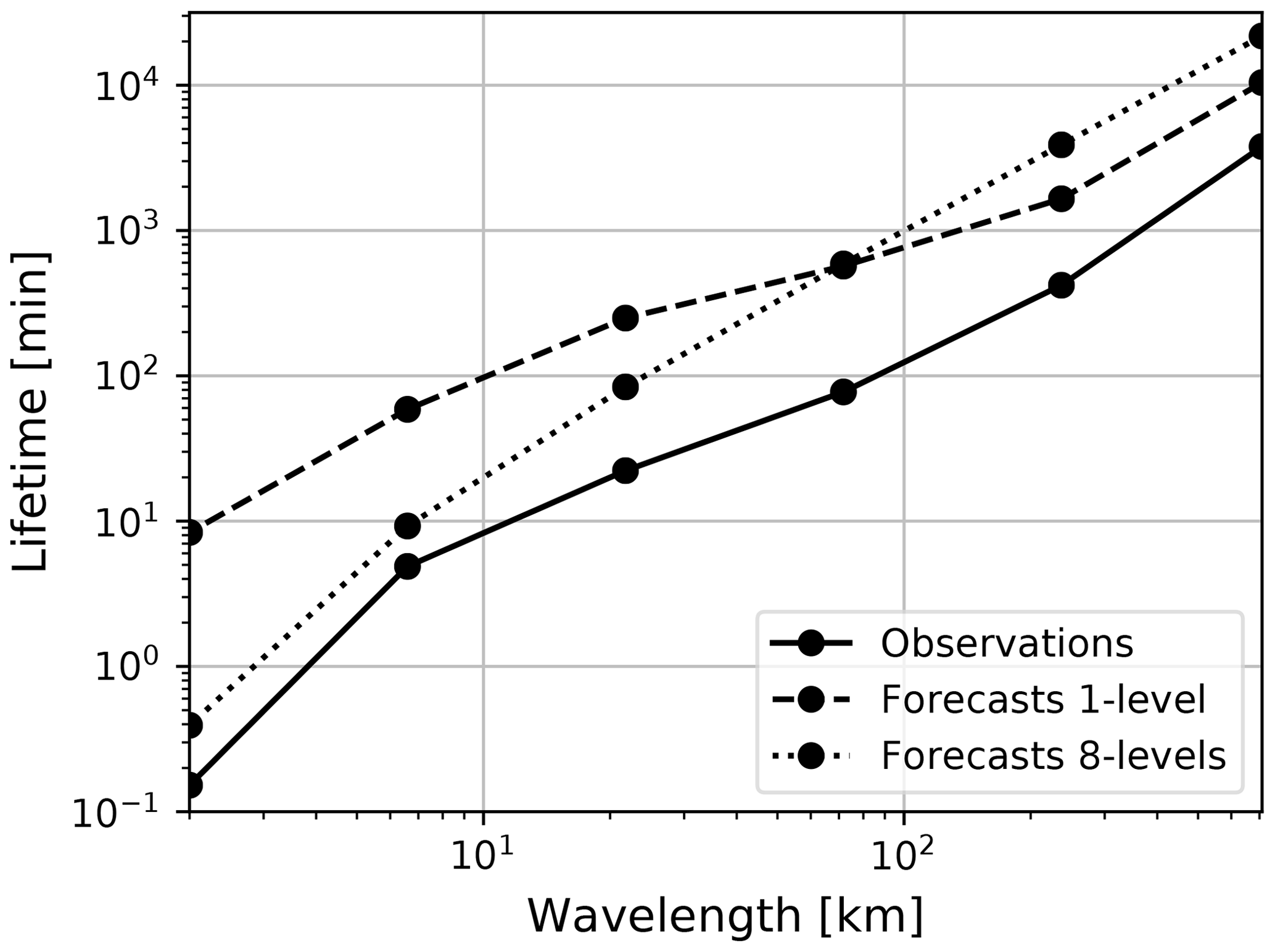
Figure 17Verification of dynamic scaling properties of stochastic nowcasts generated with one and eight cascade levels. All MeteoSwiss events were analyzed, but nowcasts were run only every 4 h.
To test our hypothesis, we compared the stochastic nowcasts (nowcasts.steps module) with and without cascade decomposition, that is, using eight or one cascade levels, respectively. The objective is to analyze the realism of the temporal evolution, not whether the AR is an appropriate model of the forecast error as in Sect. 4.6. In practice, this implies comparing the theoretical ACFs of forecast and observed fields as follows: (1) generate nowcasts with either an eight-level or one-level cascade, (2) transform the forecast fields into the Lagrangian frame (by using the same motion field estimated at start time), (3) decompose the forecast fields into a six-level cascade, (4) estimate the AR(2) parameters at each scale, (5) derive the full temporal ACF (see also Fig. 10) and (6) integrate the ACF to estimate the precipitation lifetime. The procedure is repeated for each forecast lead time up to 2 h and also for the corresponding observations.
Figure 17 shows the average lifetime for all the MeteoSwiss events plotted against spatial wavelength (in log–log scale). As expected, the model with eight cascade levels reproduces well the dynamic scaling properties, especially at small wavelengths. However, there is some degree of overestimation of the lifetime at large wavelengths compared to the observations. One possibility would be to adjust the AR parameters to obtain faster decorrelation, and thus a shorter lifetime, at such scales.
The model without cascade decomposition compensates for the overestimation of persistence at large wavelengths but strongly overestimates the one of small wavelengths. Hence, the evolution of convective cells in the stochastic nowcast is too slow compared with reality. This could be checked visually by looking at the animations of stochastic realizations with and without decomposition (*_stoch_*.gif in https://github.com/pySTEPS/pysteps-publication/tree/master/animations, last access: 23 September 2019).
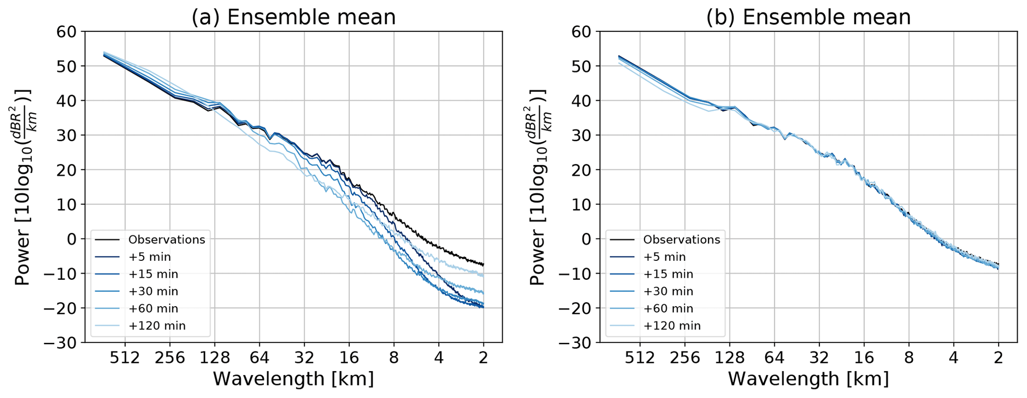
Figure 18Spatial structure analysis of the ensemble mean forecast using (a) eight cascade levels and (b) one cascade level. Both experiments have an ensemble size of 24 members. MeteoSwiss event no. 3 was used.
Another approach to understand the impact of the cascade decomposition is to analyze the filtering properties of the ensemble mean forecast (e.g., Surcel et al., 2014). Figure 18 illustrates the evolution of the ensemble mean forecast spectra with eight and one cascade levels, respectively. When using the cascade decomposition the process of ensemble averaging leads to a loss of power at small spatial wavelengths, in agreement with the expected loss of predictability (see Sect. 4.5). Instead, the model with one cascade level is not able to filter out the unpredictable features. As a consequence, it may not be able to adequately characterize the loss of predictability (and uncertainty) at different spatial scales.
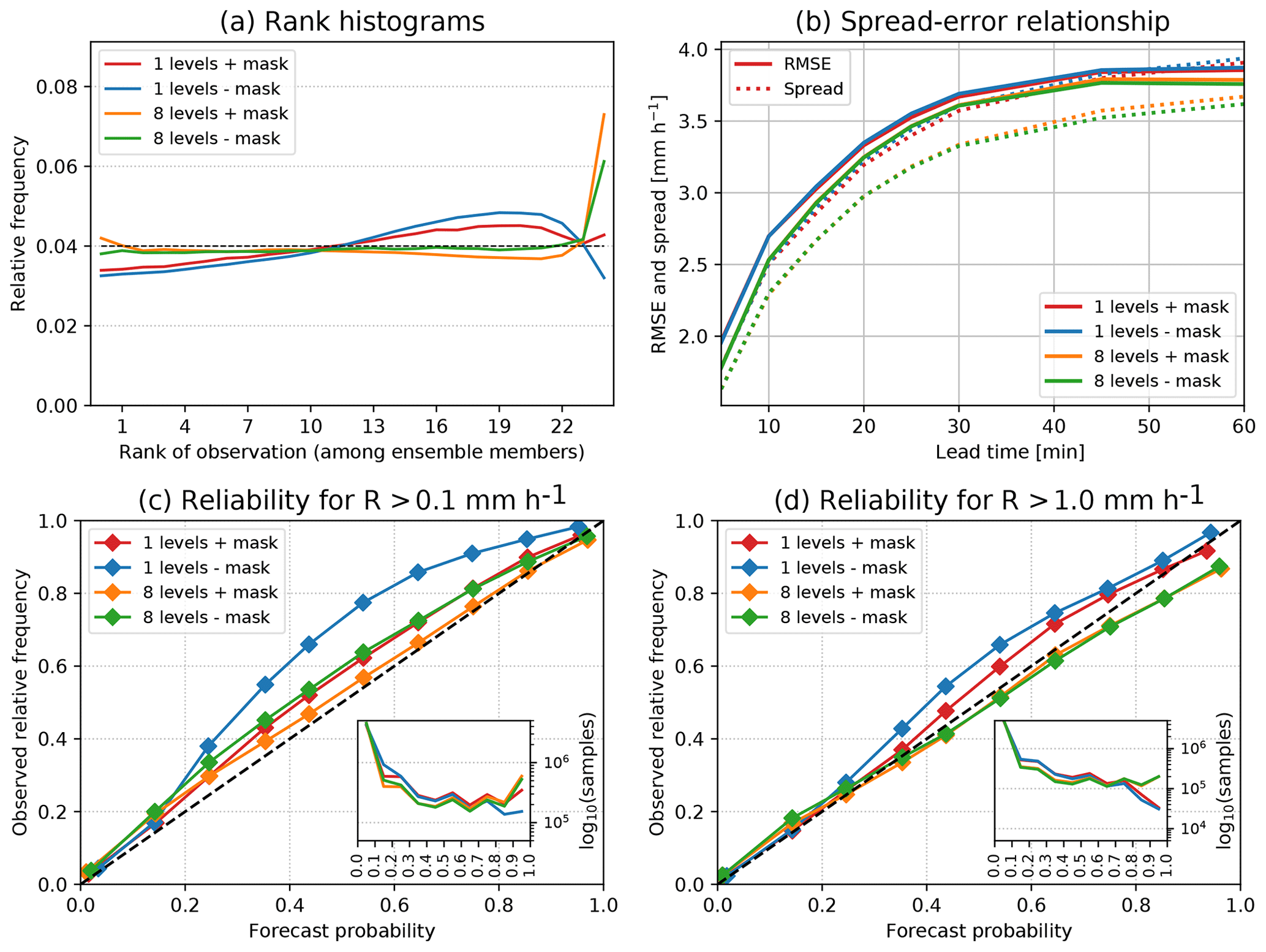
Figure 19Ensemble and probabilistic verification of the cascade experiments for all the MeteoSwiss cases with and without cascade decomposition, and with and without masking. (a) Rank histograms at 60 min, (b) spread–error relationship, (c, d) reliability diagrams at 60 min for probability of rain exceeding 0.1 and 1 mm h−1, respectively.
Figure 19 illustrates the ensemble and probabilistic verification for all the MeteoSwiss events with and without cascade decomposition. The sensitivity of forecast uncertainty estimations on using the incremental precipitation mask is also included.
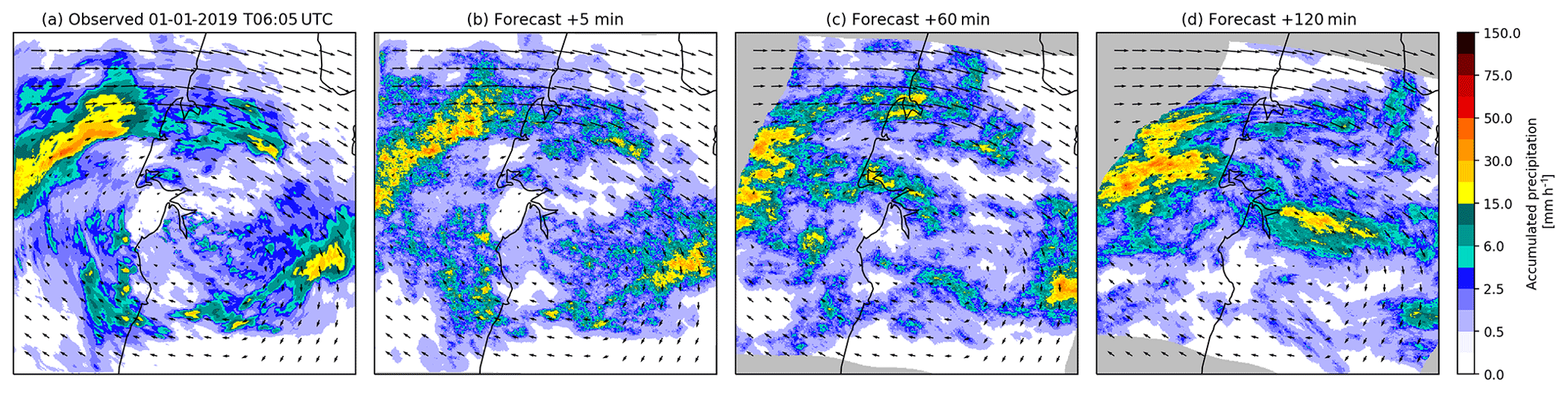
Figure 20Comparison of a member of 5 min rainfall ensemble for (b) +30 min, (c) +60 min and (d) +120 min nowcasts initialized with (a) radar-based rainfall analysis from the Australian radar network valid at 06:05 UTC on 1 January 2019 on a 512×512 pixel grid (256×256 km) (event no. 2 in Table 10).
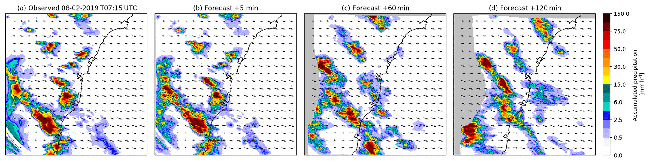
Figure 21Comparison of a member of 5 min rainfall ensemble for (b) +30 min, (c) +60 min and (d) +120 min nowcasts initialized with (a) radar-based rainfall analysis from the Australian radar network valid at 07:15 UTC on 8 February 2019 on a 512×512 pixel grid (256×256 km) (event no. 1 in Table 10).
The rank histograms behave differently depending on the chosen forecast settings (Fig. 19a). The two models without decomposition denote a clear overdispersion with a characteristic dome-shape in the bin range 13–22, especially for the setting with one level and no mask. Instead, the models with eight levels display a flat histogram, except for the very last bin, which contains the frequency of observations exceeding all the ensemble members (misses). As shown in Fig. 14, this underdispersion can be reduced by increasing the ensemble size. The last bin is also quite sensitive to using the mask, which prevents the ensemble to capture the uncertainty associated to precipitation initiation far from the main precipitation body.
Figure 19b shows the spread–error relationship analysis (i.e., the standard deviation among all ensemble members) against the average RMSE of all members against the observations. The experiments with eight levels have both a lower RMSE and spread than the ones using one level. It can also be noticed that the one-level models do not show the same overdispersion that was observed on the rank histograms.
Finally, the reliability diagrams of Fig. 19c–d demonstrate a very good reliability for all forecast settings, although the forecast probabilities of the models with one level are slightly lower than the observed frequencies. In addition, the eight-level model has better sharpness, i.e., a larger proportion of high forecast probabilities (>0.9).
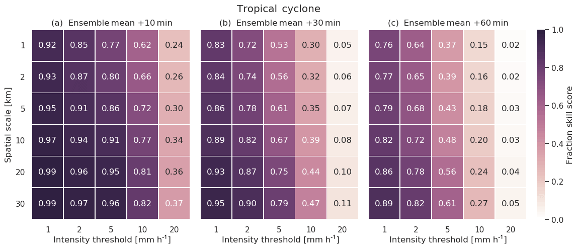
Figure 22Comparison of fractions skill score (FSS) values for (a) +10 min, (b) +30 min and (c) +60 min nowcasts rainfall ensembles for tropical cyclone Penny (event no. 1 in Table 10). FSS values were calculated comparing the ensemble mean for each lead time with observations.

An example of applying the pysteps library in order to forecast rainfall fields for tropical cyclone Penny and severe convection in Sydney (Australia) is shown in Figs. 20 and 21, respectively. The ability of pysteps to estimate diverse advection patterns from observed data is quite clear in these examples, with the tropical cyclone case showing a clear clockwise rotational pattern, while the severe convection shows an almost even easterly flow pattern across the whole domain. Tropical cyclone nowcasts preserve the original cyclonic pattern up to 60 min ahead but some distortions are induced for longer lead times due to convergence and divergence. The severe convection case has a simpler advection pattern that helps to preserve the general structure of the observed rainfall fields beyond 60 min. Additional data sources such as satellite or NWP forecasts may help to estimate future advection velocities and reduce potential anomalies for longer lead times. It is important to note, however, that post-processing of nowcasts (see Sect. 2.8) ensures that the forecast rainfall fields have the same statistical properties with the observed ones in both case studies.
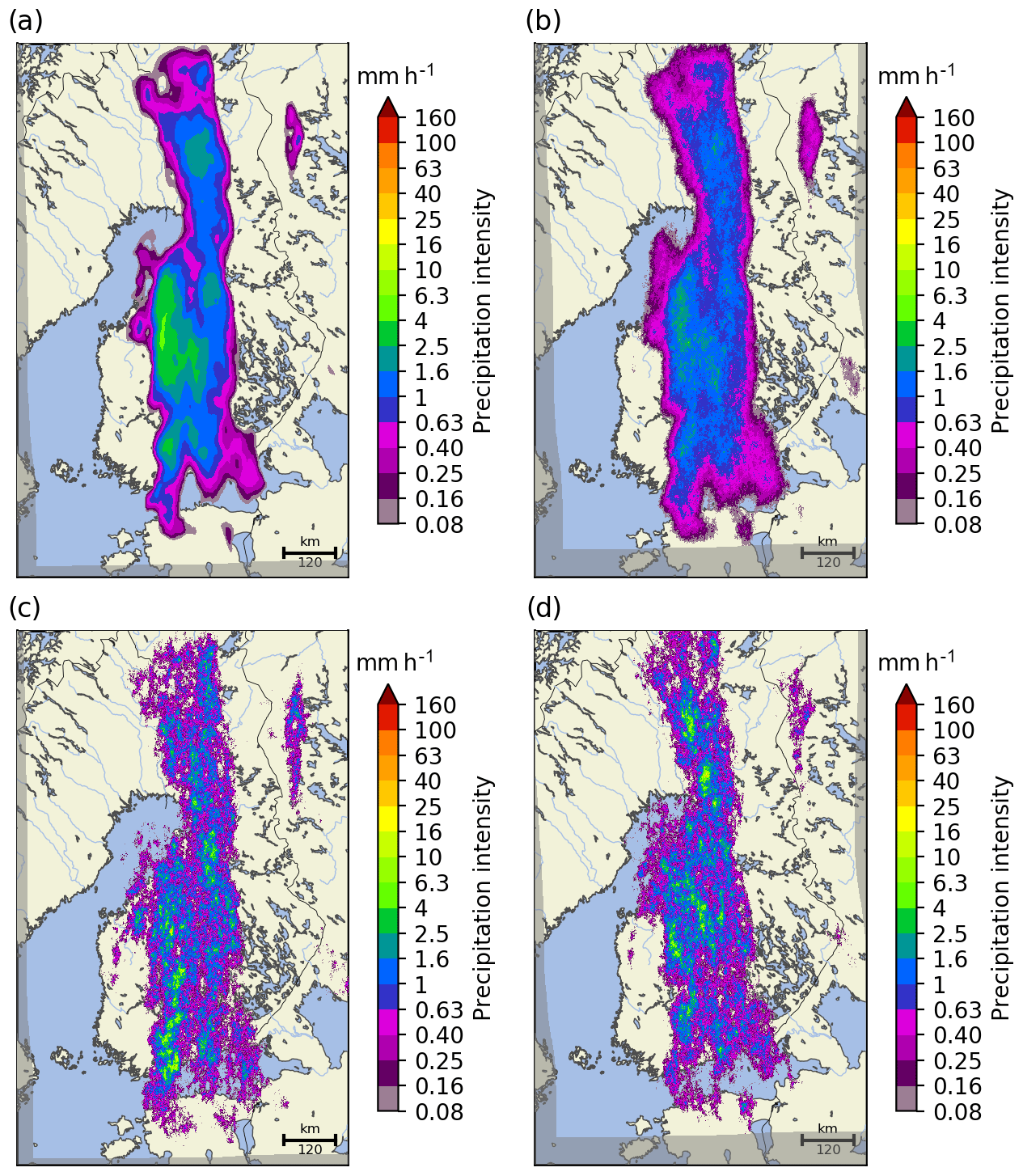
Figure 25The deterministic S-PROG nowcast (a), ensemble mean (b) and two ensemble members (c, d) of a 1 h STEPS nowcast starting at 16:00 UTC on 28 September 2016.
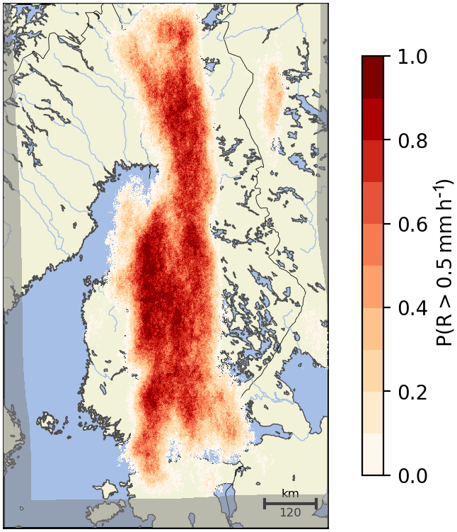
Figure 26Probability of exceeding 0.5 mm h−1 computed from the STEPS nowcast ensemble shown in Fig. 25 with 24 members.
6.1 Neighborhood verification
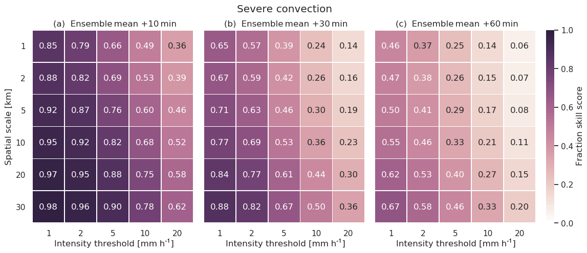
Figures 22 and 23 show examples of FSS results calculated by pysteps for different forecast times for both Australian case studies.
The FSS decays in both case studies when spatial scale is reduced or when the intensity threshold is increased, although differences exist between the two case studies. For example, the tropical cyclone case seems to have a less acute reduction in the skill with changes in spatial scale. This can be related to the presence of a more uniform rainfall distribution across the domain (large bands of rainfall moving in an organized way) limiting displacement errors at small scales. Instead, the skill reduces heavily as rainfall intensity increases. This drop in skill could have been accentuated by the relatively low number of high-intensity samples in these events.
On the other hand, the severe convection case displays a stronger decay of skill when spatial scale is reduced, probably due to the presence of sharp spatial gradients and isolated convective cells. This said, it is interesting to note how for the higher intensities and large spatial scales the FSS values do not decay as heavily as seen in the other case study. This difference could be a consequence of having more high-intensity values in the severe convection event.
Table 7Precipitation events in Finland (FMI). The duration of each event is 12 h.
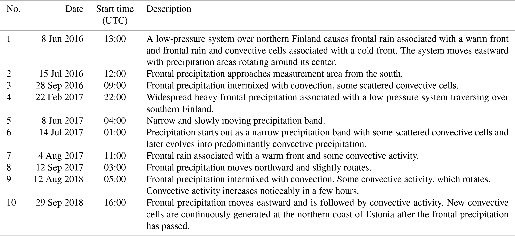
Table 8Precipitation events in Switzerland (MeteoSwiss). The duration of each event is 12 h.
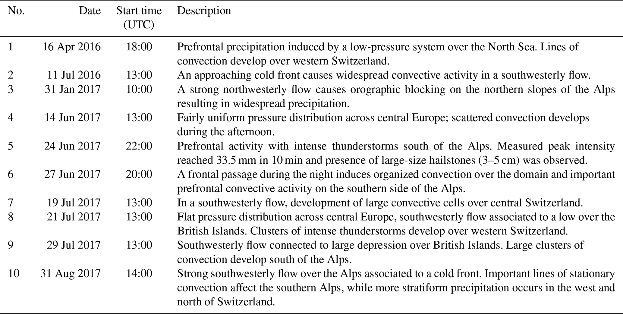
Table 9Precipitation events from the US. The duration of each event is 12 h.
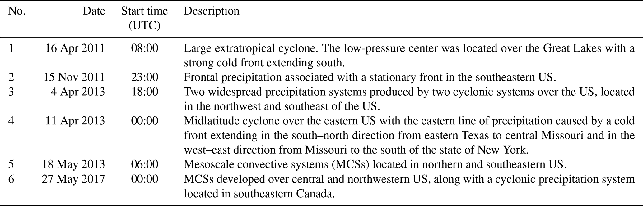
Table 10Precipitation events from Australia (BoM). The duration of each event is 12 h.
6.2 Lifetime of rainfall fields per spatial scale
To compare the behavior of the AR(2) model for these two case studies, temporal auto-correlation functions for each spatial scale were calculated using Eq. (7) and then integrated to estimate the precipitation lifetimes for each scale and runtime. Figure 24 summarizes the precipitation lifetime results for each case study. Overall, a more diverse set of spatial and temporal patterns observed during the severe convection event makes interquartile ranges of precipitation lifetimes larger for this case study for all scales. In comparison, similar organized patterns were present during most of the duration of the tropical cyclone event and therefore precipitation lifetime values have a narrower range. Smaller scales seem to have similar average lifetime values for both cases with no strong temporal variations within the events. For the larger scales, however, precipitation lifetime values for tropical cyclone event are greater than severe convection ones, again as a consequence of large-scale organized patterns observed in this event.
From an operational perspective, these results illustrate the importance of using an AR(2) model with parameters continuously adjusted to the latest observed patterns to adequately simulate rainfall nowcasts instead of using fixed, historical parameters. However, it is important to note as well that a number of outliers were obtained in both cases (mainly for the larger spatial scales). These anomalous values may indicate the need for introducing a temporal smoothing scheme during the estimation of the AR(2) parameters. Having a more stable, slowly evolving parameters would help to (i) reduce the possibility of generating unrealistic nowcasts from one particular set of observations and also (ii) create smooth transitions between consecutive rainfall nowcasts.
Pysteps is an open-source library for radar-based probabilistic precipitation nowcasting written in Python. It represents a community-based initiative that aims at connecting nowcasting scientists by sharing code, methods, ideas and results and also providing an easy-to-use tool for operational applications.
Pysteps implements the main components of an ensemble precipitation nowcasting system. These are input/output, optical flow and extrapolation routines, time series methods for modeling the temporal evolution of precipitation fields, stochastic noise generation in space and time, visualization and forecast verification.
The development of pysteps is done by using a distributed version control system, and the project is hosted on GitHub (https://pysteps.github.io, last access: 23 September 2019). The library has a modular design so that developers can easily interchange components and embed them into other software packages.
In this paper, we briefly explained the framework of probabilistic precipitation nowcasting and how such nowcasts can be produced using pysteps. The potential of pysteps was demonstrated using radar composite images from Finland (FMI), Switzerland (MeteoSwiss), the United States and Australia (BoM). Finally, we performed experiments where the quality of pysteps nowcasts and computational performance were evaluated with different configurations. This brought us to the following conclusions:
-
Probabilistic precipitation nowcasts computed with pysteps have good reliability that, however, decreases for increasing rainfall intensity thresholds and lead time. Using the MeteoSwiss data, it was shown that for the 0.1 mm h−1 threshold, reliable nowcasts with potentially useful skill can be obtained up to 3 h. When the threshold was increased to 5 mm h−1, useful nowcasts could still be obtained up to 45 min (Figs. 5 and 6).
-
Rank histograms show that the ensemble spread has a good correspondence with the nowcast uncertainty. However, we also observed some underdispersion with 10 %–15 % of observations falling outside of the 24-member ensemble verified on MeteoSwiss data (Figs. 7 and 14). This was mostly related to the inability of persistence-based nowcasting to predict the initiation of new convection (misses).
-
The stochastic ensemble members have realistic spatial and temporal structure, as confirmed by Fourier analysis (Figs. 8, 9, 10 and 17).
-
The three optical flow methods that we tested, i.e., Lucas–Kanade, DARTS and VET, provided similar forecast accuracy (differences less than 2 %; see Fig. 11). We conclude that the choice of optical flow method is not a first-order problem in terms of nowcast quality, although there may be some specific situations requiring more advanced schemes, e.g., in the presence of orographic rain and/or multiscale motion. Choosing a fast optical flow routine provides more time to generate a larger ensemble. When tested with the FMI and MeteoSwiss data, DARTS and Lucas–Kanade computed the motion field in less than 5 s.
-
With parallelization implemented via the Dask library, pysteps can generate relatively large ensembles within typical time constraints of real-time nowcasting systems. For example, by using four CPU cores on the MeteoSwiss grid (710×640), it is possible to produce a 48-member ensemble up to +1 h (12 frames) in about 2 min (Fig. 15).
-
Localizing the nowcasting procedure, that is, having spatially variable model parameters, is beneficial in terms of probabilistic forecast skill (Fig. 16). The need for localization is intuitively important for large domains, where different weather systems can coexist, but also for smaller domains that are characterized by complex orography, as it was demonstrated in this study. These results highlight the importance of defining an appropriate model domain for pysteps. That is to say, one that compromises between the need for homogeneous statistical properties (i.e., a small domain) and the need for a robust estimation of model parameters (i.e., large domain).
-
Considering the scale dependence of precipitation predictability is clearly important. The Fourier-based cascade decomposition provides an adequate framework, which can be easily extended to account for spatial localization (i.e., the short-space FFT). Other decomposition frameworks can be explored, but it is not yet clear whether there is a benefit in terms of forecast quality.
-
In the presence of extreme precipitation, pysteps can still deliver skillful nowcasts up to 1 h for specific intensity and spatial scales (Figs. 22 and 23). A wide range of predictability is observed between and within the events (Fig. 24), thus highlighting the importance of having an adaptive approach that continuously updates the model parameters in real time.
Our analyses not only helped understanding the importance of certain nowcasting concepts but were the basis to define a minimum viable product (MVP), which constitutes the default configuration of pysteps (see Table 5). Additional levels of complexity (e.g., localization) can be included at the cost of computational time and robustness. Users are responsible for evaluating whether it is worth the effort in terms of forecast quality and computational resources.
7.1 Potential extensions and applications of pysteps
Pysteps represents a long-term effort that does not end with the publication of this paper. The current pysteps version (1.0) provides a quite comprehensive library but still misses two important modules: (1) a module to generate QPE ensembles characterizing the radar measurement uncertainty (e.g., Jordan et al., 2003; Germann et al., 2009) and (2) a module for seamless blending of precipitation fields from different data sources, such as radar nowcasts and NWP forecasts (Bowler et al., 2006; Nerini et al., 2019), radar, satellite and NWP data (Renzullo et al., 2017).
It would be interesting to include other state-of-the-art ensemble precipitation nowcasting systems in pysteps, for example, PHAST (Metta et al., 2009), SBMcast (Berenguer et al., 2011), SAMPO-TBM (Leblois and Creutin, 2013), SWIRLS ensemble rainstorm nowcast (SERN; Woo and Wong, 2017) and NowPrecip (Sideris et al., 2018). A large-scale forecast verification intercomparison project could be foreseen to better understand the advantages and disadvantages of different ensemble nowcasting techniques.
Pysteps opens a number of possibilities that go beyond the field of nowcasting. The most natural application of pysteps is to use the precipitation ensembles as inputs into hydrological models for uncertainty quantification, in both urban and rural environments (e.g., Zappa et al., 2011; Thorndahl et al., 2017).
An obvious and crucial application of nowcasting systems is to support the operational warnings for rainstorms, thunderstorms and severe weather.
Individual pysteps modules can also serve different purposes. For example, the optical flow modules can be used to study precipitation growth and decay in moving coordinates (e.g., Foresti et al., 2018, 2019; Zeder et al., 2018), to correct radar field accumulations accounting for advection (e.g., Wang et al., 2015; Lukach et al., 2017), to synchronize the individual radar elevation scans (e.g., Tabary, 2007) or to separate the location error of NWP precipitation forecasts (Marzban and Sandgathe, 2010).
The tools available in the noise and the time series modules can be used for stochastic simulation of design storms (e.g., Seed et al., 1999; Paschalis et al., 2013) and weather generators (Peleg et al., 2017), and also to understand and quantify the subpixel variability of radar rainfall (e.g., Gires et al., 2014; Benoit et al., 2018; Peleg et al., 2016). Other applications can include stochastic downscaling or emulation of climate model output (e.g., Raut et al., 2018; Beusch et al., 2019).
We encourage the nowcasting community and potential users to implement new nowcasting methods, propose new modules, try pysteps on different applications, provide feedback and contribute to the library for the benefit of everyone.
The pysteps library version 1.0 is available at https://doi.org/10.5281/zenodo.2631911 (Pulkkinen et al., 2019). The scripts to run the experiments and produce the figures of this paper are available at https://doi.org/10.5281/zenodo.3458712 (Pulkkinen et al., 2019). The radar data are available upon request.
Listing A1 demonstrates how to browse and read archived radar composites using the io module and decompose a radar image into a cascade using the cascade module. The desired time stamp, root path of the data archive, the file name pattern and extension for finding the input file are specified at lines 9–12. Finding the input files is done by using io.archive.find_by_date at lines 14 and 15. Nine previous input files preceding the desired time stamp are also retrieved with the given time step of 5 min. The retrieved file names are then supplied to io.read_timeseries that returns a three-dimensional array of shape (num_timesteps,height,width) containing the radar precipitation fields and a metadata dictionary (line 19). The cascade decomposition is done by initializing the Fourier filter with filter_gaussian and calling decomposition_fft (lines 24–25).
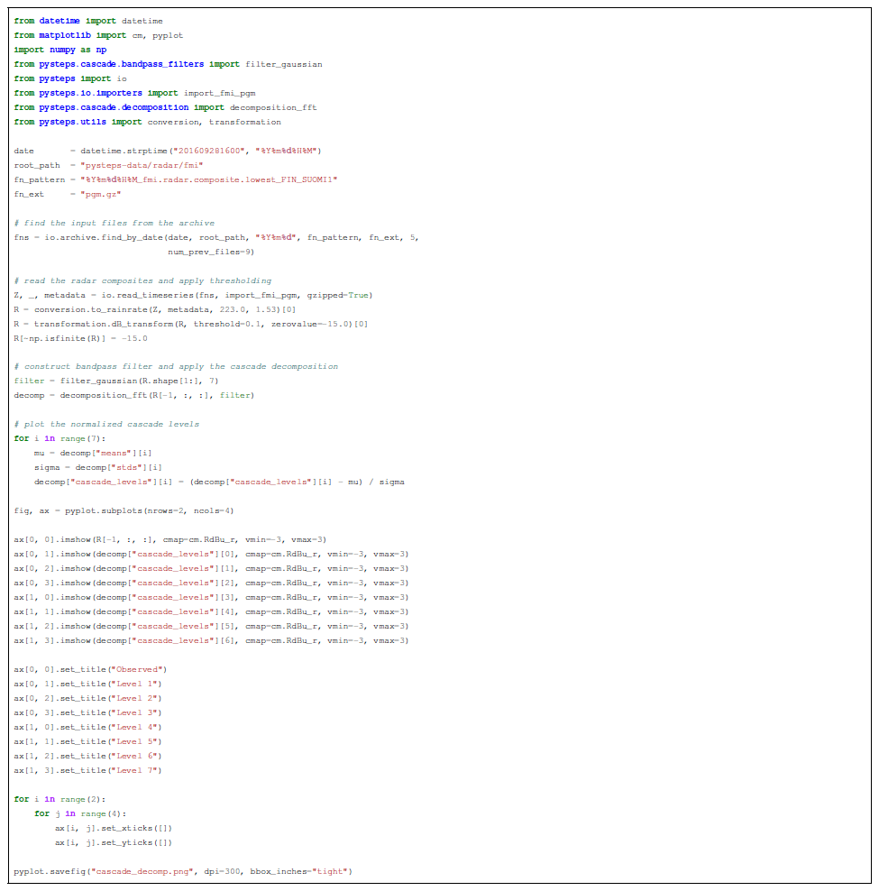
Listing A1Read 10 archived radar reflectivity composites in portable gray map (PGM) format, apply thresholding and decompose the last one into a seven-level cascade and plot the cascade levels.
Listing A2 demonstrates computation of a deterministic S-PROG nowcast and a STEPS nowcast ensemble. This is done in two stages: computation of the advection field using the Lucas–Kanade method implemented in the motion module (lines 8–9) and then computing the nowcasts with the motion field supplied as input (lines 12–18). The callable functions for these are retrieved using the get_method interface. The inputs for the nowcasting methods are a time series of three radar composites (Z), the motion field (V), the number of time steps (12), the number of cascade levels (eight) and the threshold for rain/no rain (−10 dBR). In addition, for STEPS, the ensemble size and the spatial and temporal resolution of the data are set to 24, 1 km and 5 min, respectively. The resulting nowcasts are shown in Figs. 25 and 26.
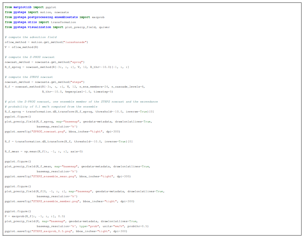
Listing A2Compute the advection field and S-PROG and STEPS nowcasts from the reflectivity composites obtained in Listing A1 and plot the nowcasts. The nowcasts are computed by using 12 time steps (i.e., 1 h nowcast with the 5 min time step), eight cascade levels and −10 dBR intensity threshold. The STEPS nowcast is computed by using 24 ensemble members.
Verification of a nowcast ensemble is shown in Listing A3 using three metrics: ROC, reliability diagram and rank histogram (see Sect. 4.2). The verifying observations are imported at lines 4–10 by using the io module. This is followed by a loop over the time steps of the nowcast. For each time step, the verification metric is initialized with the *_init function, and the verification data are accumulated to the resulting object by calling *_accum, which allows accumulating data from multiple events. In addition, exceedance probabilities (P_f) for the 0.1 mm h−1 threshold used above are computed by using ensemblestats.excprob.
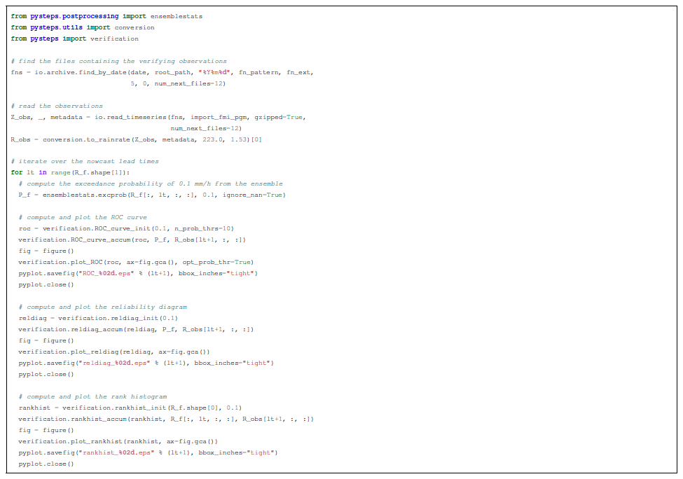
The core of the pysteps package was mainly written by SP and DN, with many contributions by AAPH. LF has promoted and closely followed the design of pysteps from its birth. The previously mentioned authors and CVF made many analyses and figures for the paper. UG and AS supported the project, supervised the science and improved the paper.
The authors do not have any competing interests.
The authors express their gratitude to Weather Decision Technologies for providing access to the United States radar composites. The whole pysteps community is also acknowledged here for the various contributions and discussions to the project.
Seppo Pulkkinen was supported by the Finnish Academy of Science and Letters. Loris Foresti and Daniele Nerini were supported by the Swiss National Science Foundation Ambizione project “Precipitation attractor from radar and satellite data archives and implications for seamless very short-term forecasting” (PZ00P2_161316). This research has been supported by the European Horizon 2020 (grant no. EC-HORIZON2020-PR700099-ANYWHERE).
This paper was edited by Richard Neale and reviewed by Wang Chun Woo and one anonymous referee.
Alfieri, L., Salamon, P., Pappenberger, F., Wetterhall, F., and Thielen, J.: Operational early warning systems for water-related hazards in Europe, Environ. Sci. Policy, 21, 35–49, 2012. a
Atencia, A. and Zawadzki, I.: A comparison of two techniques for generating nowcasting ensembles. Part I: Lagrangian ensemble technique, Mon. Weather Rev., 142, 4036–4052, 2014. a
Atencia, A., Zawadzki, I., and Berenguer, M.: Scale characterization and correction of diurnal cycle errors in MAPLE, J. Appl. Meteorol. Climatol., 56, 2561–2575, 2017. a
Ayzel, G., Heistermann, M., and Winterrath, T.: Optical flow models as an open benchmark for radar-based precipitation nowcasting (rainymotion v0.1), Geosci. Model Dev., 12, 1387–1402, https://doi.org/10.5194/gmd-12-1387-2019, 2019. a
Benoit, L., Allard, D., and Mariethoz, G.: Stochastic Rainfall Modeling at Sub-kilometer Scale, Water Resour. Res., 54, 4108–4130, 2018. a
Berenguer, M., Sempere-Torres, D., and Pegram, G. G. S.: SBMcast – An ensemble nowcasting technique to assess the uncertainty in rainfall forecasts by Lagrangian extrapolation, J. Hydrol., 404, 226–240, 2011. a, b
Berenguer, M., Surcel, M., Zawadzki, I., Xue, M., and Kong, F.: The Diurnal Cycle of Precipitation from Continental Radar Mosaics and Numerical Weather Prediction Models. Part II: Intercomparison among Numerical Models and with Nowcasting, Mon. Weather Rev., 140, 2689–2705, 2012. a
Berne, A., Delrieu, G., Creutin, J.-D., and Obled, C.: Temporal and spatial resolution of rainfall measurements required for urban hydrology, J. Hydrol., 299, 166–179, 2004. a
Beusch, L., Gudmundsson, L., and Seneviratne, S. I.: Emulating Earth System Model temperatures: from global mean temperature trajectories to grid-point level realizations on land, Earth Syst. Dynam. Discuss., https://doi.org/10.5194/esd-2019-34, in review, 2019. a
Bouguet, J.-Y.: Pyramidal implementation of the affine Lucas Kanade feature tracker description of the algorithm, Intel Corp., 5, 4, https://doi.org/10.1109/HPDC.2004.1323531, 2001. a
Bowler, N. E., Pierce, C. E., and Seed, A. W.: STEPS: A probabilistic precipitation forecasting scheme which merges an extrapolation nowcast with downscaled NWP, Q. J. Roy. Meteorol. Soc., 132, 2127–2155, 2006. a, b, c, d, e, f, g, h
Box, G. E. P., Jenkins, G. M., Reinsel, G. C., and Ljung, G. M.: Time series analysis: forecasting and control, John Wiley & Sons, New Jersey, USA, fifth Edn., 2013. a
Bradski, G.: The OpenCV Library, Dr. Dobb's Journal of Software Tools, 2000. a
Bröcker, J. and Smith, L. A.: Increasing the Reliability of Reliability Diagrams, Weather Forecast., 22, 651–661, 2007. a
Chatfield, C.: The Analysis of Time Series: An Introduction, Chapman and Hall/CRC, sixth Edn., 2003. a
Crane, R.: Space-time structure of rain rate fields, J. Geophys. Res., 95, 2011–2020, 1990. a
Dask Development Team: Dask: Library for dynamic task scheduling, available at: https://dask.org (last access: 30 July 2019), 2016. a
Erdin, R., Frei, C., and Künsch, H. R.: Data Transformation and Uncertainty in Geostatistical Combination of Radar and Rain Gauges, J. Hydrometeorol., 13, 1332–1346, 2012. a
Flowerdew, J.: IMPROVER: Integrated Model post-PROcessing and VERification, available at: https://tinyurl.com/y8m33y7l (last access: 23 September 2019), BoM Ensembles Workshop, 2018. a
Foresti, L. and Seed, A.: The effect of flow and orography on the spatial distribution of the very short-term predictability of rainfall from composite radar images, Hydrol. Earth Syst. Sci., 18, 4671–4686, https://doi.org/10.5194/hess-18-4671-2014, 2014. a
Foresti, L., Reyniers, M., Seed, A., and Delobbe, L.: Development and verification of a real-time stochastic precipitation nowcasting system for urban hydrology in Belgium, Hydrol. Earth Syst. Sci., 20, 505–527, https://doi.org/10.5194/hess-20-505-2016, 2016. a, b
Foresti, L., Sideris, I., Panziera, L., Nerini, D., and Germann, U.: A 10-year radar-based analysis of orographic precipitation growth and decay patterns over the Swiss Alpine region, Q. J. Roy. Meteorol. Soc., 144, 2277–2301, 2018. a
Foresti, L., Sideris, I., Nerini, D., Beusch, L., and Germann, U.: Using a 10-year radar archive for nowcasting precipitation growth and decay – a probabilistic machine learning approach, Weather Forecast., https://doi.org/10.1175/WAF-D-18-0206.1, in press, 2019. a, b
Frigo, M. and Johnson, S. G.: The Design and Implementation of FFTW3, Proc. IEEE, 93, 216–231, 2005. a
Germann, U. and Zawadzki, I.: Scale-Dependence of the Predictability of Precipitation from Continental Radar Images, Part I: Description of the Methodology, Mon. Weather Rev., 130, 2859–2873, 2002. a, b, c, d, e
Germann, U. and Zawadzki, I.: Scale Dependence of the Predictability of Precipitation from Continental Radar Images, Part II: Probability Forecasts, J. Appl. Meteorol., 43, 74–89, 2004. a
Germann, U., Galli, G., Boscacci, M., and Bolliger, M.: Radar precipitation measurement in a mountainous region, Q. J. Roy. Meteorol. Soc., 132, 1669–1692, 2006a. a
Germann, U., Zawadzki, I., and Turner, B.: Predictability of precipitation from continental radar images. Part IV: Limits to prediction, J. Atmos. Sci., 63, 2092–2108, 2006b. a, b, c
Germann, U., Berenguer, M., Sempere-Torres, D., and Zappa, M.: REAL-Ensemble radar precipitation estimation for hydrology in a mountainous region, Q. J. Roy. Meteorol. Soc., 135, 445–456, 2009. a
Germann, U., Boscacci, M., Gabella, M., and Sartori, M.: Peak performance – Radar design for prediction in the Swiss Alps, Meteorol. Technol. Int., 42–45, 2015. a
Gires, A., Tchiguirinskaia, I., Schertzer, D., Schellart, A., Berne, A., and Lovejoy, S.: Influence of small scale rainfall variability on standard comparison tools between radar and rain gauge data, Atmos. Res., 138, 125–138, 2014. a
Haiden, T., Kann, A., Wittmann, C., Pistotnik, G., Bica, B., and Gruber, C.: The Integrated Nowcasting through Comprehensive Analysis (INCA) System and Its Validation over the Eastern Alpine Region, Weather Forecast., 26, 166–183, 2011. a
Hamill, T. M.: Interpretation of Rank Histograms for Verifying Ensemble Forecasts, Mon. Weather Rev., 129, 550–560, 2001. a
Hamill, T. M. and Colucci, S. J.: Verification of Eta-RSM Short-Range Ensemble Forecasts, Mon. Weather Rev., 125, 1312–1327, 1997. a
Hamilton, J. D.: Time Series Analysis, Princeton University Press, Princeton, New Jersey, USA, 1994. a, b
Harris, D., Seed, A., Menabde, M., and Austin, G.: Factors affecting multiscaling analysis of rainfall time series, Nonlin. Processes Geophys., 4, 137–156, https://doi.org/10.5194/npg-4-137-1997, 1997. a
Heistermann, M., Jacobi, S., and Pfaff, T.: Technical Note: An open source library for processing weather radar data (wradlib), Hydrol. Earth Syst. Sci., 17, 863–871, https://doi.org/10.5194/hess-17-863-2013, 2013. a, b
Heistermann, M., Collis, S., Dixon, M. J., Giangrande, S., Helmus, J. J., Kelley, B., Koistinen, J., Michelson, D. B., Peura, M., Pfaff, T., and Wolff, D. B.: The emergence of open-source software for the weather radar community, B. Am. Meteorol. Soc., 96, 117–128, 2015. a
Helmus, J. J. and Collis, S. M.: The Python ARM Radar Toolkit (Py-ART), a Library for Working with Weather Radar Data in the Python Programming Language, J. Open Res. Softw., 4, e25, https://doi.org/10.5334/jors.119, 2016. a
Hunter, J. D.: Matplotlib: A 2D graphics environment, Comput. Sci. Eng., 9, 90–95, https://doi.org/10.1109/MCSE.2007.55, 2007. a
Hutton, C., Wagener, T., Freer, J., Han, D., Duffy, C., and Arheimer, B.: Most computational hydrology is not reproducible, so is it really science?, Water Resour. Res., 52, 7548–7555, 2016. a
Jacques, D., Michelson, D., Caron, J.-F., and Fillion, L.: Latent Heat Nudging in the Canadian Regional Deterministic Prediction System, Mon. Weather Rev., 146, 3995–4014, 2018. a
Jolliffe, I. T. and Stephenson, D. B.: Forecast Verification: A Practitioner's Guide in Atmospheric Science, John Wiley & Sons, Chichester, UK, 2003. a, b, c, d
Jones, E., Oliphant, T., and Peterson, P.: SciPy: Open source scientific tools for Python, available at: http://www.scipy.org/ (last access: 30 July 2019), 2001. a
Jordan, P., Seed, A., and Weinmann, P.: A Stochastic Model of Radar Measurement Errors in Rainfall Accumulations at Catchment Scale, J. Hydrometeorol., 4, 841–855, 2003. a
Koistinen, J. and Pohjola, H.: Estimation of Ground-Level Reflectivity Factor in Operational Weather Radar Networks Using VPR-Based Correction Ensembles, J. Appl. Meteorol. Climatol., 53, 2394–2411, 2014. a
Lakshmanan, V., Smith, T., Hondl, K., Stumpf, G. J., and Witt, A.: A Real-Time, Three-Dimensional, Rapidly Updating, Heterogeneous Radar Merger Technique for Reflectivity, Velocity, and Derived Products, Weather Forecast., 21, 802–823, 2006. a
Lakshmanan, V., Fritz, A., Smith, T., Hondl, K., and Stumpf, G.: An Automated Technique to Quality Control Radar Reflectivity Data, J. Appl. Meteorol. Climatol., 46, 288–305, 2007. a
Laroche, S. and Zawadzki, I.: A Variational Analysis Method for Retrieval of Three-Dimensional Wind Field from Single-Doppler Radar Data, J. Atmos. Sci., 51, 2664–2682, 1994. a
Leblois, E. and Creutin, J. D.: Space-time simulation of intermittent rainfall with prescribed advection field: Adaptation of the turning band method, Water Resour. Res., 49, 3375–3387, 2013. a
Leinonen, J., Moisseev, D., Leskinen, M., and Petersen, W. A.: A Climatology of Disdrometer Measurements of Rainfall in Finland over Five Years with Implications for Global Radar Observations, J. Appl. Meteorol. Climatol., 51, 392–404, 2012. a
Liguori, S. and Rico-Ramirez, M. A.: A review of current approaches to radar-based quantitative precipitation forecasts, Int. J. River Basin Manag., 12, 391–402, 2014. a
Lorenz, E. N.: Predictability: a problem partly solved, in: Predict. Weather Clim., edited by: Palmer, T. and Hagedora, R., 40–58 pp., Cambridge University Press, 1996. a, b
Lovejoy, S. and Schertzer, D.: The Weather and Climate: Emergent Laws and Multifractal Cascades, Cambridge University Press, 2013. a
Lucas, B. D. and Kanade, T.: An iterative image registration technique with an application to stereo vision, in: Proceedings of the 1981 DARPA Imaging Understanding Workshop, 121–130 pp., 1981. a
Lukach, M., Foresti, L., Giot, O., and Delobbe, L.: Estimating the occurrence and severity of hail based on 10 years of observations from weather radar in Belgium, Meteorol. Appl., 24, 250–259, 2017. a
Mandapaka, P. V., Germann, U., Panziera, L., and Hering, A.: Can lagrangian extrapolation of radar fields be used for precipitation nowcasting over complex alpine orography?, Weather Forecast., 27, 28–49, 2012. a
Marzban, C. and Sandgathe, S.: Optical flow for verification, Weather Forecast., 25, 1479–1494, 2010. a
Mejsnar, J., Sokol, Z., and Minářová, J.: Limits of precipitation nowcasting by extrapolation of radar reflectivity for warm season in Central Europe, Atmos. Res., 213, 288–301, 2018. a
Met Office: Cartopy: a cartographic python library with a Matplotlib interface, Exeter, Devon, available at: http://scitools.org.uk/cartopy (last access: 30 July 2019), 2010–2015. a
Metta, S., von Hardenberg, J., Ferraris, L., Rebora, N., and Provenzale, A.: Precipitation nowcasting by a spectral-based nonlinear stochastic model, J. Hydrometeorol., 10, 1285–1297, 2009. a
Mittermaier, M. and Roberts, N.: Intercomparison of Spatial Forecast Verification Methods: Identifying Skillful Spatial Scales Using the Fractions Skill Score, Weather Forecast., 25, 343–354, 2010. a
Nerini, D., Besic, N., Sideris, I., Germann, U., and Foresti, L.: A non-stationary stochastic ensemble generator for radar rainfall fields based on the short-space Fourier transform, Hydrol. Earth Syst. Sci., 21, 2777–2797, https://doi.org/10.5194/hess-21-2777-2017, 2017. a, b, c
Nerini, D., Foresti, L., Leuenberger, D., Robert, S., and Germann, U.: A reduced-space ensemble Kalman filter approach for flow-dependent integration of radar extrapolation nowcasts and NWP precipitation ensembles, Mon. Weather Rev., 147, 987–1006, 2019. a
Paschalis, A., Molnar, P., Fatichi, S., and Burlando, P.: A stochastic model for high-resolution space-time precipitation simulation, Water Resour. Res., 49, 8400–8417, 2013. a
Pegram, G. G. and Clothier, A. N.: High resolution space-time modelling of rainfall: The “String of Beads” model, J. Hydrol., 241, 26–41, 2001. a, b
Peleg, N., Francesco, M., Fatichi, S., Paschalis, A., Molnar, P., and Burlando, P.: Spatial variability of extreme rainfall at radar subpixel scale, J. Hydrol., 556, 922–933, 2016. a
Peleg, N., Fatichi, S., Paschalis, A., Molnar, P., and Burlando, P.: An advanced stochastic weather generator for simulating 2‐D high‐resolution climate variables, J. Adv. Model. Earth Syst., 9, 1595–1627, 2017. a
Pérez, F. and Granger, B. E.: IPython: a System for Interactive Scientific Computing, Comput. Sci. Eng., 9, 21–29, 2007. a
Pierce, C., Seed, A., Ballard, S., Simonin, D., and Li, Z.: Nowcasting, in: Doppler Radar Observations – Weather Radar, Wind Profiler, Ionospheric Radar, and Other Advanced Applications, edited by: Bech, J. and Chau, J. L., 97–142 pp., InTech, 2012. a
Pulkkinen, S., Chandrasekar, V., and Harri, A.-M.: Nowcasting of Precipitation in the High-Resolution Dallas-Fort Worth (DFW) Urban Radar Remote Sensing Network, IEEE J. Sel. Top. Appl. Earth Obs. Remote Sens., 11, 2773–2787, 2018. a
Pulkkinen, S., Nerini, D., Perez Hortal, A., Velasco, C., and Foresti, L.: (2019, April 7), pySTEPS/pysteps: pysteps 1.0.0 (Version v1.0.0), Zenodo, https://doi.org/10.5281/zenodo.2631911, 2019.
Raut, B., Seed, A., Reeder, M., and Jakob, C.: A multiplicative cascade model for high-resolution space-time downscaling of rainfall, J. Geophys. Res.-Atmos., 123, 2050–2067, 2018. a
Renzullo, L., Velasco-Forero, C., and Seed, A.: Blending radar, NWP and satellite data for real-time ensemble rainfall analysis: a scale-dependent method, Tech. Rep. EP174236, CSIRO, https://doi.org/10.4225/08/594eb78c96025, 2017. a
Ruzanski, E., Chandrasekar, V., and Wang, Y.: The CASA Nowcasting System, J. Atmos. Ocean. Technol., 28, 640–655, 2011. a
Schertzer, D. and Lovejoy, S.: Physical modeling and analysis of rain and clouds by anisotropic scaling multiplicative processes, J. Geophys. Res., 92, 9693–9714, 1987. a
Scovell, R.: Application of the wavelet transform for modelling non-stationarity and local anisotropy in precipitation fields, in: 11th International Workshop on Precipitation in Urban Areas, Pontresina, Switzerland, 2018. a
Seed, A., Shrikanthan, R., and Menabde, M.: A space and time model for design storm rainfall, J. Geophys. Res., 104, 31623–31630, 1999. a
Seed, A. W.: A Dynamic and Spatial Scaling Approach to Advection Forecasting, J. Appl. Meteor., 42, 381–388, 2003. a, b, c, d, e, f, g
Seed, A. W., Pierce, C. E., and Norman, K.: Formulation and evaluation of a scale decomposition-based stochastic precipitation nowcast scheme, Water Resour. Res., 49, 6624–6641, 2013. a, b, c, d
Sideris, I. V., Foresti, L., Germann, U., and Nerini, D.: Nowprecip: an algorithm for localized probabilistic precipitation nowcasting in the complex terrain of Switzerland, in: Proceedings of the 10th European Conference on Radar in Meteorology and Hydrology (ERAD), Ede-Wageningen, The Netherlands, 2018. a, b
Simonin, D., Pierce, C., Roberts, N., Ballard, S., and Li, Z.: Performance of Met Office hourly cycling NWP-based nowcasting for precipitation forecasts, Q. J. Roy. Meteorol. Soc., 143, 2862–2873, 2017. a
Sun, J., Xue, M., Wilson, J. W., Zawadzki, I., Ballard, S. P., Onvlee-Hooimeyer, J., Joe, P., Barker, D. M., Li, P.-W., Golding, B., Xu, M., and Pinto, J.: Use of NWP for Nowcasting Convective Precipitation: Recent Progress and Challenges, B. Am. Meteorol. Soc., 95, 409–426, 2014. a
Surcel, M., Zawadzki, I., and Yau, M.: On the filtering properties of ensemble averaging for storm-scale precipitation forecasts, Mon. Weather Rev., 142, 1093–1105, 2014. a, b, c
Tabary, P.: The new French operational radar rainfall product, Part I: Methodology, Weather Forecast., 22, 393–408, 2007. a
Thorndahl, S., Einfalt, T., Willems, P., Nielsen, J. E., ten Veldhuis, M.-C., Arnbjerg-Nielsen, K., Rasmussen, M. R., and Molnar, P.: Weather radar rainfall data in urban hydrology, Hydrol. Earth Syst. Sci., 21, 1359–1380, https://doi.org/10.5194/hess-21-1359-2017, 2017. a
Tippett, M. K., DelSole, T., and Barnston, A. G.: Reliability of Regression-Corrected Climate Forecasts, J. Climate, 27, 3393–3404, 2014. a
Toth, Z. and Kalnay, E.: Ensemble forecasting at NCEP and the breeding method, Mon. Weather Rev., 125, 3297–3319, 1997. a
Turner, B. J., Zawadzki, I., and Germann, U.: Predictability of Precipitation from Continental Radar Images, Part III: Operational Nowcasting Implementation (MAPLE), J. Appl. Meteorol., 43, 231–248, 2004. a
Van Der Walt, S., Colbert, S. C., and Varoquaux, G.: The NumPy Array: A Structure for Efficient Numerical Computation, Comput. Sci. Eng., 13, 22–30, https://doi.org/10.1109/MCSE.2011.37, 2011. a
Venugopal, V., Foufoula-Georgiou, E., and Sapozhnikov, V.: Evidence of dynamic scaling in space-time rainfall, J. Geophys. Res.-Atmos., 104, 31599–31610, 1999. a
Wang, L.-P., Ochoa-Rodriguez, S., Van Assel, J., Pina, R., Pessemier, M., Kroll, S., Willems, P., and Onof, C.: Enhancement of radar rainfall estimates for urban hydrology through optical flow temporal interpolation and Bayesian gauge-based adjustment, J. Hydrol., 531, 408–426, 2015. a
Wang, Y., Coning, E. D., Harou, A., Jacobs, W., Joe, P., Nikitina, L., Roberts, R., Wang, J., and Wilson, J.: Guidelines for nowcasting techniques, available at: https://library.wmo.int/opac/doc_num.php?explnum_id=3795 (last access: 23 September 2019), 2017. a
Wong, W.-K., Cheng, V. T.-L., and Woo, W.-C.: Community SWIRLS Nowcasting System (Com-SWIRLS), in: WMO WWRP 4th International Symposium on Nowcasting and Very-short-range Forecast (WSN16), p. 113, available at: http://wsn16.hk/doc/wsn16-abstract-book.pdf (last access: 23 September 2019), 2016. a
Woo, W.-C. and Wong, W.-K.: Operational application of optical flow techniques to radar-based rainfall nowcasting, Atmosphere, 8, 48, 2017. a
Xingjian, S., Chen, Z., Wang, H., Yeung, D., Wong, W., and Woo, W.: Convolutional LSTM network: A machine learning approach for precipitation nowcasting, in: Neural Information Processing Systems 28, edited by: Cortes, C., Lawrence, N. D., Lee, D. D., Sugiyama, M., and Garnett, R., 802–810 pp., Curran Associates, Inc., 2015. a
Zappa, M., Simon, J., Germann, U., Walser, A., and Fundel, F.: Superposition of three sources of uncertainties in operational flood forecasting chains, Atmos. Res., 100, 246–262, 2011. a
Zawadzki, I., Morneau, J., and Laprise, R.: Predictability of Precipitation Patterns: An Operational Approach, J. Appl. Meteor., 33, 1562–1571, 1994. a
Zeder, J., Hamann, U., Nerini, D., Foresti, L., Clementi, L., Hering, A., and Germann, U.: Comparison of thunderstorm characteristics as seen by SEVIRI and radar regarding lightning and hail initiation, in: EUMETSAT conference, Tallinn, Estonia, 2018. a
- Abstract
- Introduction
- Formulation of precipitation nowcasting
- The pysteps library
- Evaluation of nowcast quality
- Sensitivity analysis
- Nowcasting the extremes: two severe-weather case studies from Australia
- Conclusions
- Code and data availability
- Appendix A: Pysteps use cases
- Appendix B: Precipitation events
- Author contributions
- Competing interests
- Acknowledgements
- Financial support
- Review statement
- References