The Brazilian Earth System Model ocean–atmosphere (BESM-OA) version 2.5: evaluation of its CMIP5 historical simulation

The performance of the coupled ocean–atmosphere component of the Brazilian Earth System Model version 2.5 (BESM-OA2.5) was evaluated in simulating the historical period 1850–2005. After a climate model validation procedure in which the main atmospheric and oceanic variabilities were evaluated against observed and reanalysis datasets, the evaluation specifically focused on the mean climate state and the most important large-scale climate variability patterns simulated in the historical run, which was forced by the observed greenhouse gas concentration. The most significant upgrades in the model's components are also briefly presented here. BESM-OA2.5 could reproduce the most important large-scale variabilities, particularly over the Atlantic Ocean (e.g., the North Atlantic Oscillation, the Atlantic Meridional Mode, and the Atlantic Meridional Overturning Circulation), and the extratropical modes that occur in both hemispheres. The model's ability to simulate such large-scale variabilities supports its usefulness for seasonal climate prediction and in climate change studies.

1 Introduction

Climate models, which have recently been expanded into Earth system models via inclusion of biogeochemical cycles, are key tools for investigating climate phenomena that significantly influence human societies (e.g., von Storch, 2010; Flato, 2011). Since 2008, the Brazilian climate community has been engaged in setting up the Brazilian Earth System Model (BESM; Nobre et al., 2013; Giarolla et al., 2015). This major scientific task has been carried out by Brazilian scientific institutions and highlights the critical need to produce reliable future climate projections and to understand their potential impact, particularly over South America. The primary objective of this effort was to assemble the scientific expertise capable of developing and maintaining a state-of-the-art Earth system model. Such an achievement would represent a significant step forward in establishing a scientific tool that can be used in different types of research activities. The importance of such an undertaking lies in the need to understand the physics of the Earth system to produce and lend credibility to studies that explore the impacts of climate change on different areas of great importance, such as food and water security, tropical ecosystems, and natural disasters. One of the fundamental aims of the BESM project is to participate in the Coupled Model Intercomparison Project's sixth phase (CMIP6; Meehl et al., 2014).

BESM has been set up at the Brazilian National Institute for Space Research (INPE). Currently, it consists of a land–ocean–atmosphere coupled model in which the coupling is achieved via the FMS coupler, a tool developed at the Geophysical Fluid Dynamics Laboratory (GFDL) of the National Oceanic and Atmospheric Administration (NOAA). The inclusion of aerosols (as read-in fields) and atmospheric chemistry components is in the implementation and testing phases. Currently, work has been completed to activate the biogeochemical model, TOPAZ, within the Modular Ocean Model version 5 (MOM5) to simulate biogeochemical cycles in future simulations.

The previous version of BESM (BESM-OA2.3) was first evaluated by Nobre et al. (2013). This version showed a significant bias against precipitation in the tropical region, as it showed a deficient representation of the precipitation in the Amazon region. To improve these aspects, studies were conducted to ameliorate cloud parameterizations over the tropics, and the resulting changes improved the representation of the precipitation over the same region and the representation of Convergence Zones over both the Atlantic and Pacific Ocean basins (Bottino and Nobre, 2019). The main changes in the current version of BESM relate to its atmospheric model, which now incorporates modifications in the surface wind field and its parameterizations as described in Capistrano et al. (2018). The updated version presented in this paper is BESM-OA2.5.

Operationally, BESM-OA2.3 is already being used for extended weather forecasting (10–30 d) and for seasonal climate prediction (3 months), as well as for producing global climate change scenarios (Nobre et al., 2013) and providing atmospheric and oceanic boundary conditions to regional climate models for dynamical downscaling of climate change scenarios (Chou et al., 2014).

This overview paper describes the most important developments and improvements in the model's components, and presents the simulation of recent-past mean climate conditions and major large-scale climate phenomena. In Sect. 2, the BESM-OA2.5 components and experimental design are briefly described; Sect. 3 presents the methodology and the observed data used to evaluate the model; Sect. 4 presents the evaluation of the historical simulation, which evaluated the most important atmospheric and oceanic variables related to their climatological fields and the prominent large-scale phenomena of the climate system; and, finally, Sect. 5 provides a summary.

2 Model description and experimental design of the simulation

2.1 BESM-OA2.5

The atmospheric component of BESM-OA2.5 is the Brazilian Global Atmospheric Model (BAM; Figueroa et al., 2016), which was developed at the Center for Weather Forecasting and Climate Studies (CPTEC/INPE). The BAM is a primitive equation model with spectral representation with triangular truncation at the wavenumber 62 (corresponding to a grid resolution of approximately $\mathrm{1.875}{}^{\circ }\times \mathrm{1.875}{}^{\circ }$) and 28σ levels in the vertical, with uneven increments between the levels, i.e., a T62L28 resolution. As mentioned before, it is the atmospheric component that underlies the primary differences between BESM-OA2.5 and BESM-OA2.3 (Nobre et al., 2013). The new version includes a key improvement in the energy balance at the top of the atmosphere via reduction of the mean global bias from −20 W m⁻² in version BESM-OA2.3 to −4 W m⁻² in the current version (Capistrano et al., 2018). BESM version 2.5 incorporates the formulation presented in Jiménez et al. (2012) for representing the wind, humidity, and temperature in the surface layer. The model runs without flux correction or adjustment. The physics parameterizations for the continental processes are based on the Simplified Simple Biosphere Model (SSiB) land surface model (Xue et al., 1991), the shortwave radiation is based on the CLIRAD scheme (Chou and Suarez, 1999; Tarasova and Fomin, 2000), the longwave radiation is based on the Harshvardhan scheme (Harshvardhan et al., 1987), the cloud microphysics uses the Ferrier scheme (Ferrier et al., 2002), the vertical diffusion is the modified MY2.0 scheme (Mellor and Yamada, 1982), the gravity wave drag scheme is based on Webster et al. (2003), the deep convection module is based on Grell and Dévényi (2002), and the shallow convection module is based on Tiedtke (1983). More details can be found in Figueroa et al. (2016) and Capistrano et al. (2018).

The oceanic component of BESM-OA2.5 is the Modular Ocean Model version 4p1 (MOM4p1; Griffies, 2009) developed at GFDL, which includes the Sea Ice Simulator (SIS) built-in ice model (Winton, 2000). There were no changes in the physics parameterizations used in BESM-OA2.3. The horizontal grid resolution in the zonal direction is 1^∘; in the meridional direction it varies uniformly from 1∕4^∘ between 10^∘ S and 10^∘ N to 1^∘ of resolution at 45^∘ and to 2^∘ of resolution at 90^∘ (in both hemispheres). The vertical resolution has 50 levels, with approximately 10 m resolution in the upper 220 m and increasing gradually to about 370 m resolution at deeper levels. The oceanic model spin-up was performed in a manner similar to that of Nobre et al. (2013) and Giarolla et al. (2015), in which the spin-up run begins from rest, and the ocean T–S structure is that of Levitus (1982). The initial stage of the ocean model spin-up was performed over a 13-year period, forced by climatological atmospheric fields (winds, solar radiation, air temperature and humidity, and precipitation). The model spin-up was then integrated by an additional 58-year period, forced by interannually varying atmospheric fields from Large and Yeager (2009), while maintaining the river discharges and the sea ice variables at their respective monthly mean climatological values. The forced ocean model run was used to save the oceanic dynamical and thermodynamical structures to be used for initiating future coupled model experiments.

The atmospheric and oceanic models were coupled via the FMS coupler, which was also developed at GFDL and incorporated into MOM4p1. The atmospheric model receives sea surface temperature (SST) and ocean albedo data from the ocean and sea ice models at hourly time increments. The oceanic model receives information about freshwater (liquid and solid precipitation), momentum fluxes (winds at 10 m), specific humidity, heat, vertical diffusion of velocity components, and surface pressure, also at hourly time increments. The wind stress fields were computed in MOM4p1 using the Monin–Obukhov scheme (Obukhov, 1971). In the coupled simulations, the ocean temperature and salinity restoration options were set to off.

2.2 Experimental design

A set of numerical experiments were performed with the coupled ocean–atmosphere version of BESM-OA2.5 following the CMIP5 experimental design protocol (Taylor et al., 2012), and they are shown schematically in Fig. 1. Out of the experiments listed below, only the historical simulation is evaluated in this paper. The following experiments were performed:

• Historical. The simulation ran over the period 1850–2005 (156 years), forced by the observed historical atmospheric equivalent CO₂ concentration (greenhouse gas only) over this period, and based on the CMIP5 protocol.

• piControl. Ran for 1140 years, forced by the invariant pre-industrial atmospheric CO₂ concentration level (280 ppmv).

• Abrupt 4xCO2. Ran for 1000 years, consisting of an abrupt quadruplication of the atmospheric CO₂ concentration level from the piControl simulation.

• RCP4.5. Ran over the period 2006–2105 (100 years), forced by the time-dependent changes in greenhouse gas levels projected by the Representative Concentration Pathway 4.5 (RCP4.5), based on the CMIP5 protocol. This simulation continued the historical simulation through the 21st century, reaching a radiative atmospheric forcing of 4.5 W m⁻² in 2100.

• RCP8.5. The same as the RCP4.5 simulation, but forced by the time-dependent changes in greenhouse gas levels projected by the Representative Concentration Pathway 8.5 (RCP8.5), based on the CMIP5 protocol, i.e., reaching a radiative atmospheric forcing of 8.5 W m⁻² in 2100.

The ocean stand-alone component ran for 71 years (a 13-year period of ocean model spin-up forced by climatological atmospheric fields plus a 58-year period forced by interannually varying atmospheric fields). Next, a spin-up of the fully coupled model was performed for 100 years. The oceanic and atmospheric states at the end of this 100-year-long integration were used as the initial conditions for the piControl simulation. The versions of the model differ slightly in the 100-year spin-up and the piControl run, i.e., in the parameterizations of the land ice albedo and in the cloud microphysics. For its initial conditions, the historical simulation used information about the 14th year provided by the piControl simulation. The piControl simulation showed stable conditions following a fast adjustment over the first 13 years of simulation (figure not shown). Therefore, it is assumed that the historical simulation had a spin-up of 113 years. The analyses of the piControl and 4xCO2 simulations are described in Capistrano el al. (2018). Capistrano et al. (2018) estimated that BESM-OA2.5 has an equilibrium climate sensitivity of 2.96 ^∘C in the abrupt 4xCO2 experiment. This value is within the range of 2.07 to 4.74 ^∘C that was computed for 25 CMIP5 models and is close to the ensemble averaged value (3.30 ^∘C).

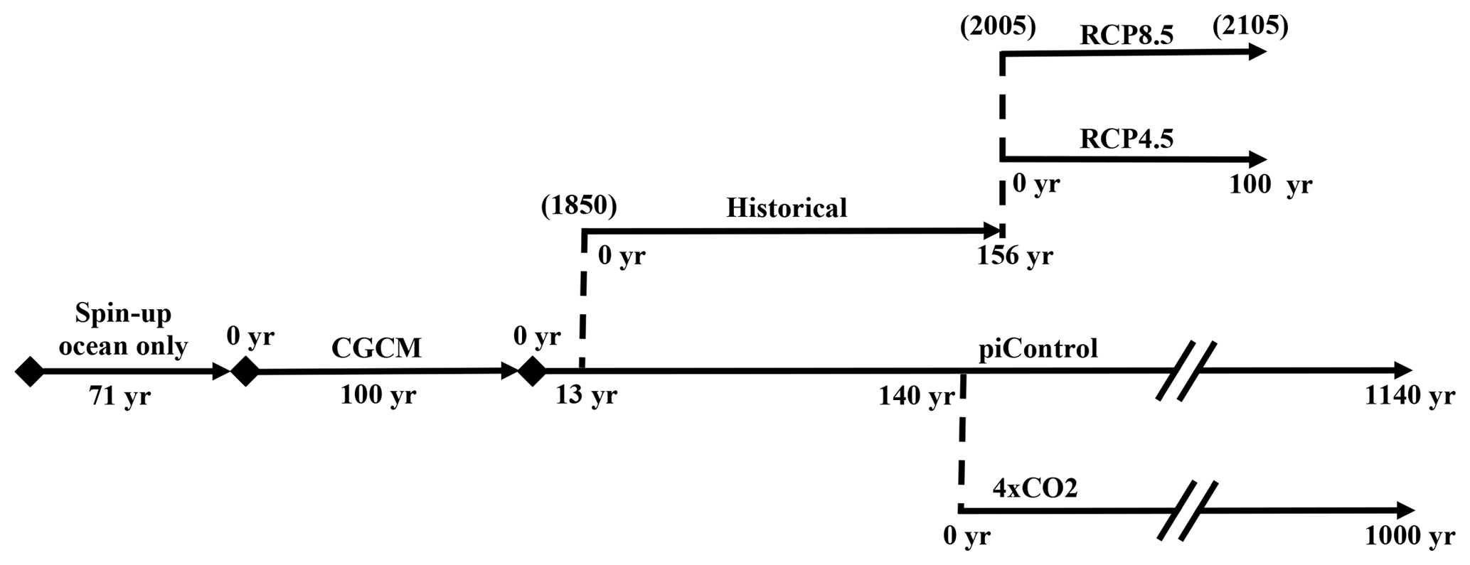
Figure 1 A scheme of the principal simulations carried out by BESM-OA2.5 using different forcing conditions based on the CMIP5 protocols. The dates for the historical and RCP simulations are from the actual calendar years.

3 Methods and data

To evaluate the output of the BESM-OA2.5 historical simulation, comparisons were made against the observed datasets and reanalysis products. The atmospheric fields and sea ice concentration were from the Twentieth Century Reanalysis dataset version 2 (20CRv2; Compo et al., 2011) with a global horizontal resolution of $\mathrm{2}{}^{\circ }\times \mathrm{2}{}^{\circ }$ and 24 vertical levels (https://www.esrl.noaa.gov/psd/data/gridded/data.20thC_ReanV2.html, last access: 27 February 2019); the precipitation dataset was obtained from the Global Precipitation Climatology Project version 2.2 Combined Precipitation Dataset (GPCP; Adler et al., 2003; Huffman et al., 2009) with a global horizontal resolution of $\mathrm{2.5}{}^{\circ }\times \mathrm{2.5}{}^{\circ }$ (http://rda.ucar.edu/datasets/ds728.2/#!description, last access: 19 February 2019) and from the Climate Prediction Center Merged Analysis of Precipitation (CMAP; Xie and Arkin, 1997), with a global horizontal resolution of $\mathrm{2.5}{}^{\circ }\times \mathrm{2.5}{}^{\circ }$ (https://www.esrl.noaa.gov/psd/data/gridded/data.cmap.html, last access: 27 February 2019). To compare the global average air surface temperature, the Hadley Centre – Climate Research Unit temperature anomalies version 4 (HadCRUT4; Morice et al., 2012), which provides a time series of the globally averaged air temperature anomaly at 2 m (https://crudata.uea.ac.uk/cru/data/temperature/, last access: 19 February 2019) was used. The cloud cover was compared to data from the International Satellite Cloud Climatology Project (ISCCP D2; Rossow and Schiffer, 1999), which has a global horizontal resolution of $\mathrm{2.5}{}^{\circ }\times \mathrm{2.5}{}^{\circ }$ (https://isccp.giss.nasa.gov/products/onlineData.html, last access: 27 February 2019). Finally, for the SST comparisons, the Extended Reconstructed Sea Surface Temperature version 4 (ERSSTv4; Huang et al., 2015), which is available at a grid resolution of $\mathrm{2}{}^{\circ }\times \mathrm{2}{}^{\circ }$, was used (https://www.esrl.noaa.gov/psd/data/gridded/data.noaa.ersst.v4.html, last access: 27 February 2019).

To identify the main modes of climate variability, all of the analyses presented in the paper were performed using detrended dataset anomalies. Detrended datasets were obtained by removing the linear trend based on a least-squares regression. For the analyses using monthly datasets, the annual cycle was removed by subtracting the climatological monthly means from the respective individual months. Prior to performing the analyses, the model's datasets were interpolated to the grid resolution of the respective observation or the reanalysis datasets used for comparison.

The empirical orthogonal function analysis (EOF; Hannachi et al., 2007) was used to analyze the model's ability to simulate major modes of climate variability and to compare them with observations. Prior to performing the EOF calculations, the data were weighted by the square root of the cosine of latitude. The results of the EOF maps are shown as the original data anomalies regressed onto the normalized principal component (PC) time series, i.e., by the standard deviation.

In this paper, to evaluate the periodicity of the phenomena, the power spectrum technique based on Fourier analysis of the normalized time series was applied, in which the normalization was based on the long-term monthly standard deviation.

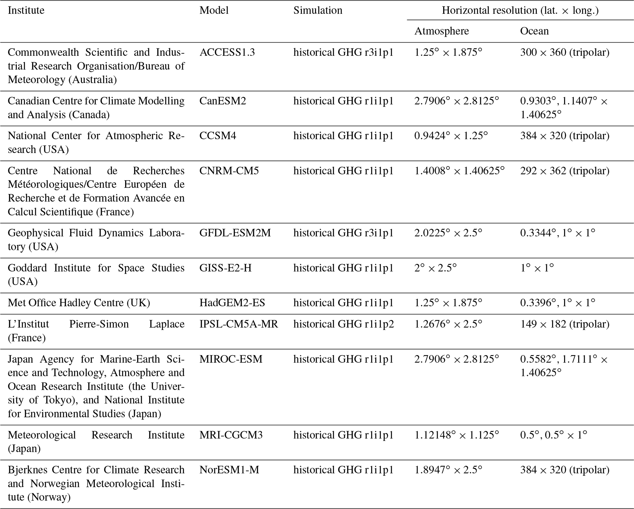
To gain better insight into the performance of BESM-OA2.5 in relation to the global average near-surface air temperature and the average SST in the equatorial regions of the Pacific and Atlantic Ocean, a comparison with 11 CMIP5 models was performed (Table 1). Because the BESM-OA2.5 historical simulation is forced only by the observed CO₂ equivalent concentration, the historical simulation forced only by greenhouse gas (historical greenhouse gas, GHG) was chosen for this comparison.

Table 1 List of the models from CMIP5 with historical GHG simulations used for the comparison with BESM-OA2.5. Models with higher resolution in the tropical region and decreasing resolution towards the poles have two values for latitude in their respective oceanic resolution columns. For models with oceanic tripolar grids, the number of grid points in each coordinate are given.

4 Results

4.1 Mean climate state

In this section, the most important atmospheric and oceanic variables are evaluated in relation to their climatological fields, either globally or over regions in which their representations are key elements of the climate system.

4.1.1 Mean surface air temperature

The evolution of the global surface air temperature during the industrial era is a key element for analyzing the long-term model behavior while being forced by the observed conditions. The HadCRUT4 observation and BESM-OA2.5 time series of the globally averaged air temperature anomaly at 2 m are shown in Fig. 2. The time series are the annual mean anomalies relative to the period from 1850 to 1879. The BESM-OA2.5 simulation of the global average surface air temperature evolution closely followed the observed time series. However, since BESM-OA2.5 does not incorporate the representation of aerosols, and consequently their cooling effects, the surface air warming rate should be higher, similar to the remaining models (the grey shading in Fig. 2). To compare BESM-OA2.5 with the selected CMIP5 models, the grey shading represents the spread of the minimum and the maximum values of the yearly anomalies from the 11 models (Table 1). In this comparison, the historical GHG simulation was used, in which the models are only forced by well-mixed greenhouse gases (mainly carbon dioxide, methane, and nitrous oxide), without the cooling resulting from the direct and indirect effects of aerosols, volcanos, and effects of land use change. Thus, the CMIP5 models show a warmer tendency compared with the observations (see Jones et al., 2013, for more details). Although BESM-OA2.5 has the same forcing conditions, it does not show the warming tendency seen in the remaining models. With the exception of GFDL-ESM2M (1861–2005) and HadGEM2-ES (1860–2005), all of the remaining CMIP5 models encompass the period from 1850 to 2005, and their respective anomalies are from the period 1850 to 1879. For GFDL-ESM2M and HadGEM2-ES, the anomalies are computed relative to the periods 1861–1890 and 1860–1889, respectively.

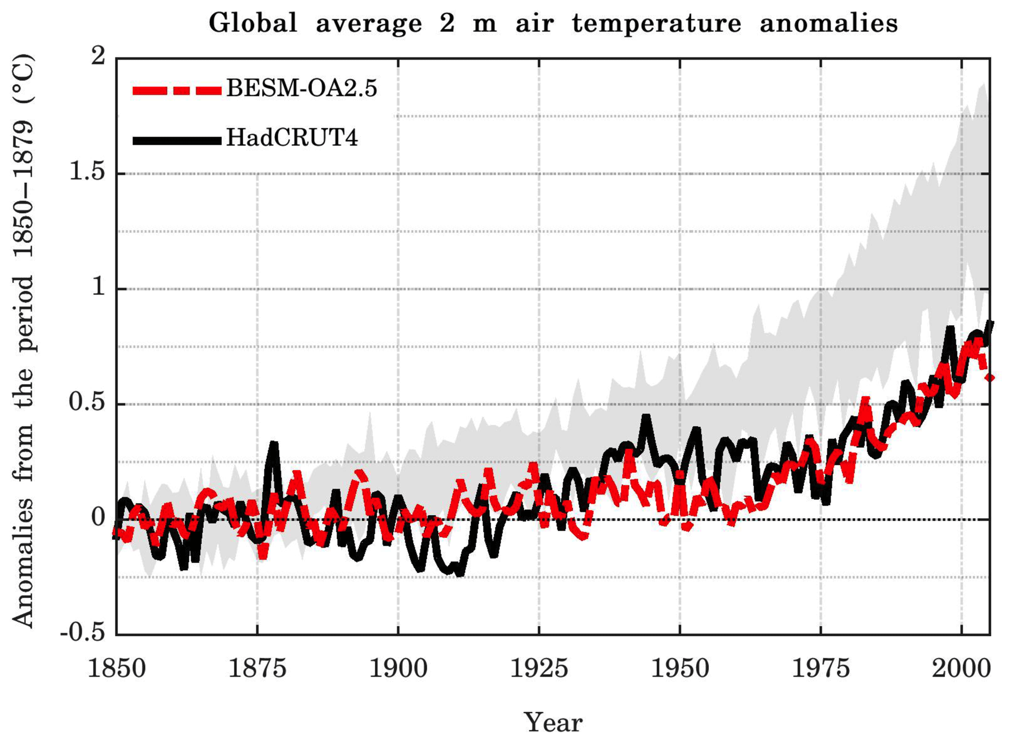
Figure 2 Global averaged 2 m annual mean air temperature anomalies relative to the period 1850–1879 as simulated by BESM-OA2.5 (dashed red line) and observed (solid black line). The grey shading represents the spread of 11 CMIP5 models (historical GHG simulations). The CMIP5 model anomalies were also computed relative to the period 1850–1879, with the exception of GFDL-ESM2M and HadGEM2-ES whose anomalies were computed relative to the periods 1861–1890 and 1860–1889, respectively. Units are in degrees Celsius.

The net radiation at the top of atmosphere (TOA) has a negative bias and the net ocean/atmosphere heat flux has a positive bias (Fig. 3). The net TOA radiation has a mean value of −4.20 W m⁻², and the net ocean/atmosphere heat flux has a mean value of 1.16 W m⁻² over the first 50 years. The net radiation imbalance at the TOA is related to a significant loss of energy at the TOA both from outgoing longwave radiation and outgoing shortwave radiation. Throughout the simulation, the net radiation at the TOA becomes less negative due to the increasing CO₂ in the atmosphere and the consequential increase in the atmospheric heat content. Part of this heat is transferred into the ocean, as indicated by the positive net increase in the ocean/atmosphere heat flux. The negative net radiation at the TOA and the positive ocean/atmosphere heat flux are likely the reasons for the weak warming observed in the historical simulation (Fig. 2), as the atmosphere loses heat to outer space and into the oceans during the simulation.

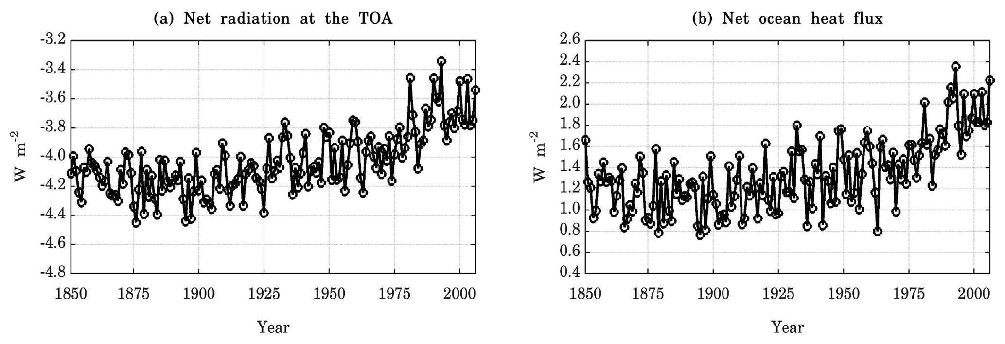
Figure 3 Annual average time series for the global average (a) net radiation at the TOA (positive values indicate that the atmosphere is warming) and (b) net ocean/atmosphere heat flux (positive values indicate that the ocean is warming), as simulated by the historical run over the period 1850–2005 (156 years). Units are in watts per square meter.

4.1.2 Mean precipitation

One of the key points in evaluating a climate model is to gauge its ability to simulate the hydrological cycle, as this cycle is critical for maintaining the energy balance of the climate system. Figure 4 shows the spatial distribution of annual mean precipitation for (a) BESM-OA2.5, (b) the GPCP dataset, (c) the spatial distribution of annual mean precipitation bias for BESM-OA2.5 relative to the GPCP dataset, and (d) for BESM-OA2.5 relative to the CMAP dataset. The spatial annual mean precipitation values represent averaged values over the periods 1971–2000 and 1979–2008 for BESM-OA2.5, and the GPCP and CMAP datasets, respectively. The global model's mean biases are similar for GPCP (0.3 mm d⁻¹) and CMAP (0.4 mm d⁻¹). In the case of the global model's root-mean-square error (RMSE) biases, they are also similar for GPCP (1.4 mm d⁻¹) and CMAP (1.5 mm d⁻¹). BESM-OA2.5 was able to reproduce the globally observed precipitation patterns and showed a slight improvement in the global mean precipitation simulation over the previous version (BESM-OA2.3). The spatial average biases were 0.3 and 0.5 mm d⁻¹, and the RMSE biases were 1.4 and 1.7 mm d⁻¹ for BESM-OA2.5 and BESM-OA2.3, respectively. The improvements are particularly clear in the Pacific and Atlantic Ocean areas, where BESM-OA2.5 reduced the positive bias that extends into the subtropical southeast Pacific and into both north and south Atlantic subtropics that was observed in BESM-OA2.3 (see Fig. 6a of Nobre et al., 2013). Despite these improvements, BESM-OA2.5 still generated a strong negative bias over the Amazon region. This is a particular concern since an important aim is related to the model's usefulness for future climate projections in that region. Based on the progress observed from BESM-OA2.3 to BESM-OA2.5, work on cloud parameterizations to improve the precipitation simulation over the Amazon is still needed. Nevertheless, some state-of-the-art models show deficiencies in generating precipitation over the Amazon region. This is the case of the IITM-ESM (Fig. 5; Swapna et al., 2018), although the bias is more confined to the north of the Amazon, and for the NESMv3, which has a more distributed bias over the region (Fig. 9; Cao et al., 2018). The Indian subcontinent region also has a significant negative bias, and a strong positive bias appears over the Indian Ocean and in the South Pacific Convergence Zone (SPCZ). Such strong positive biases over the Indian Ocean (near the African coast) are also identified in different versions of the CCSM model (Fig. 5; Gent et al., 2011).

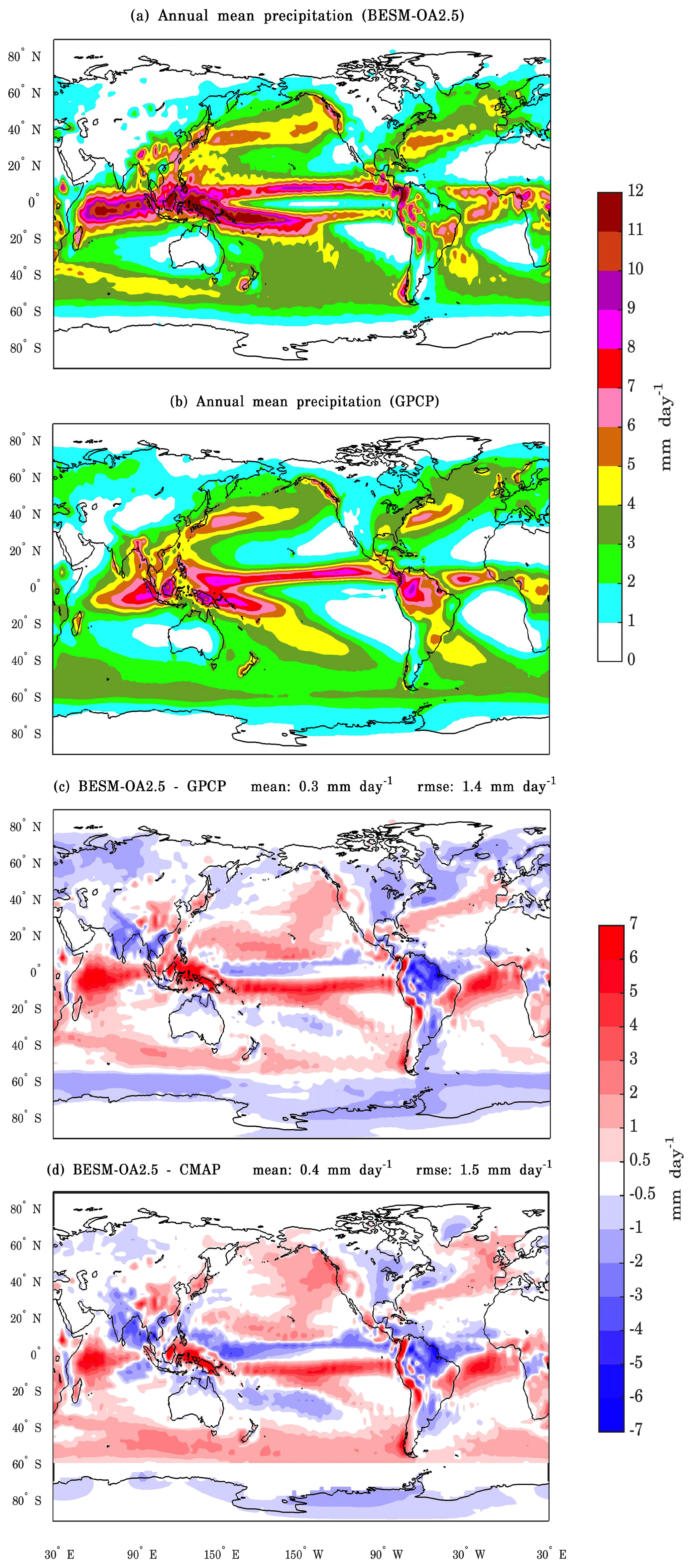
Figure 4 Spatial maps of the annual mean precipitation for (a) BESM-OA2.5, (b) GPCP, (c) the bias of BESM-OA2.5 relative to GPCP, and (d) the bias of BESM-OA2.5 relative to CMAP. The average values were computed over the periods 1971–2000 (for BESM-OA2.5) and 1979–2008 (for GPCP and CMAP). Units are in millimeters per day.

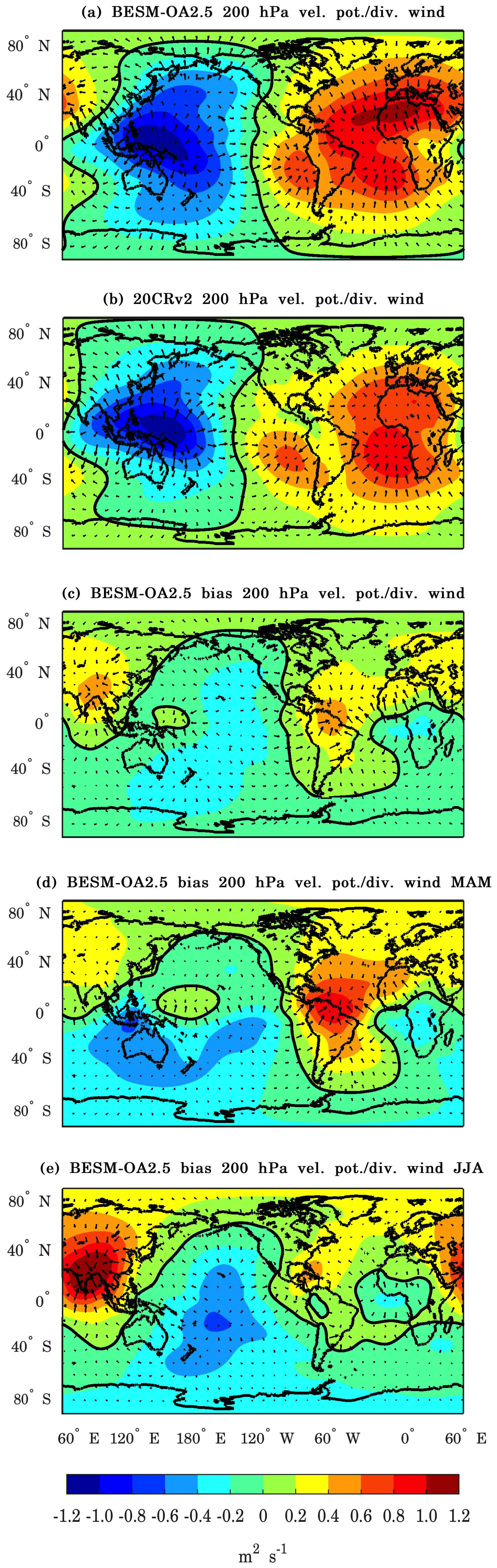
Figure 5 Spatial maps showing the averaged global anomalies in velocity potential and wind divergence at the 200 hPa pressure level for (a) BESM-OA2.5 and (b) 20CRv2 reanalysis. (c) The bias of the model relative to the reanalysis; (d) and (e) are the biases for the MAM and JJA seasons, respectively. The averages were computed over the period 1950–2005. Units are in meters per second.

To understand the global atmospheric circulation associated with the precipitation deficiencies over both the Amazon and Indian regions, the global anomalies of the velocity potential and the divergence of the wind at the 200 hPa pressure level were computed and are shown in Fig. 5. The velocity potential and divergent wind anomalies were averaged over the period 1971–2000 for the BESM-OA2.5 outputs (Fig. 5a), the 20CRv2 reanalysis (Fig. 5b), and for the difference BESM-OA2.5 minus reanalysis (Fig. 5c, d, and e). Figure 5c shows anomalous convergence over the Amazonian and Indian regions resulting in the model's poor capacity in creating convection and, consequently, to generate precipitation. Figure 5d and e show the velocity potential and wind divergence separated by season. For the Amazonian rainfall season, which occurs during MAM, it is possible to observe anomalous convergence at high levels of the atmosphere (Fig. 5d). An equivalent result was observed for the Indian region during the JJA season (Fig. 5e).

Figure 6 shows the zonally averaged precipitation during the four seasons. For this comparison, the results of the BESM-OA2.3 analysis performed by Nobre et al. (2013) are also shown. Both versions could reproduce the maximum peaks of precipitation in both the tropical and subtropical regions. BESM-OA2.5 showed a negative bias from around 40^∘ latitude poleward in both hemispheres. In the seasons DJF, JJA, and SON, BESM-OA2.5 had a positive bias on the peak of maximum precipitation corresponding to the Intertropical Convergence Zone (ITCZ). During the MAM season, the model still failed to perform the interhemispheric transition of the ITCZ. However, the JJA season showed that BESM-OA2.5 could completely perform the transition, whilst BESM-OA2.3 showed a double ITCZ in the JJA and SON seasons. The double ITCZ problem is one of the most significant biases that persists in climate models (e.g., Hwang and Frierson, 2013; Li and Xie, 2014; Tian, 2015). With the exception of the MAM season, BESM-OA2.5 yielded zonal precipitation values that were identical to the observed values, although with a generally positive bias. It should be noted that BESM-OA2.5 has a rapid precipitation decline at high latitudes. Compared to the GPCP dataset, the model showed peaks of precipitation at midlatitudes, which are related to the storm tracks, and less precipitation in the subtropics.

Figure 6 Zonally averaged annual mean precipitation for the BESM-OA2.5, BESM-OA2.3, and GPCP datasets relative to the seasons DJF, MAM, JJA, and SON. The zonally averaged values were computed over the periods 1971–2000 and 1979–2008 for BESM-OA2.5 and GPCP, respectively. Units are in millimeters per day.

Figure 7 shows the general characteristics of cloudiness over the globe simulated by the model. In particular, Fig. 7a shows that the model underestimated cloudiness in most parts of the globe, with significant exceptions in the high latitudes of the boreal hemisphere and in the southern subequatorial regions of the Pacific and Atlantic oceans upon comparison with observations. Globally, BESM-OA2.5 has a cloudiness negative bias of −13.9 % with a RMSE of 19.9 %. The periods used were 1971–2000 and 1984–2009 for BESM-OA2.5 and ISCCP, respectively. The model failed to generate clouds in the high latitudes of the austral hemisphere, as can be observed in Fig. 7b, where the percentage of cloud cover is negligible. The reason for this lack of simulated cloudiness in this region is not yet clear. However, Fig. 7b shows that the meridional variation in cloud cover simulated by the model is similar to the observation.

Figure 7 (a) Spatial map of annual mean total cloud fraction bias of BESM-OA2.5 relative to ISCCP. (b) Zonally averaged total cloud cover for the BESM-OA2.5 and ISCCP datasets. The periods used were 1971–2000 and 1984–2009 for BESM-OA2.5 and ISCCP, respectively. Units are in percent.

4.1.3 Zonal atmospheric mean state

Figures 8 and 9 present the analysis of the zonally averaged vertical profiles of air temperature and zonal wind for all seasons as simulated by BESM-OA2.5 and the respective bias relative to the 20CRv2 reanalysis dataset, in which all of the data are time averaged over the period 1971–2000. BESM-OA2.5 had a large positive air temperature bias that appears above the 250 hPa pressure level (Fig. 8) in the subpolar and polar regions during all of the seasons. This result indicates that the model warms abnormally in the tropopause and the lower stratosphere in the polar regions. The warm bias is stronger during the DJF and MAM seasons over the northern polar region, reaching a maximum bias of 20 ^∘C during the DJF season. Such a bias is a matter of concern since other models, despite showing strong bias in the polar regions, do not show such a strong bias. BNU-ESM presents positive biases up to 10 ^∘C in the austral hemisphere during the season JJA (Fig. 3a; Ji et al., 2014) and NorESM1-M presents negative biases ($\sim -\mathrm{10}$ ^∘C) during the DJF and JJA seasons (Fig. 9; Bentsen et al., 2013). In the lower and middle troposphere, BESM-OA2.5 showed a negative temperature bias that is stronger in the lower troposphere over the polar region in the respective winter–spring seasons in both hemispheres, i.e., during DJF and MAM over the North Pole, and JJA and SON over the South Pole. This negative bias reached its maximum of −10 ^∘C over the South Pole during SON. Such a negative bias in the troposphere has already been reported by many CMIP5 models (see Charlton-Perez et al., 2013; Tian et al., 2013).

Figure 8 Contour lines showing the zonally averaged vertical air temperatures for BESM-OA2.5 and the difference between the BESM-OA2.5 and 20CRv2 datasets are shaded. Both are averaged over the period 1971–2000. The units are in degrees Celsius and the contour interval is 10 ^∘C.

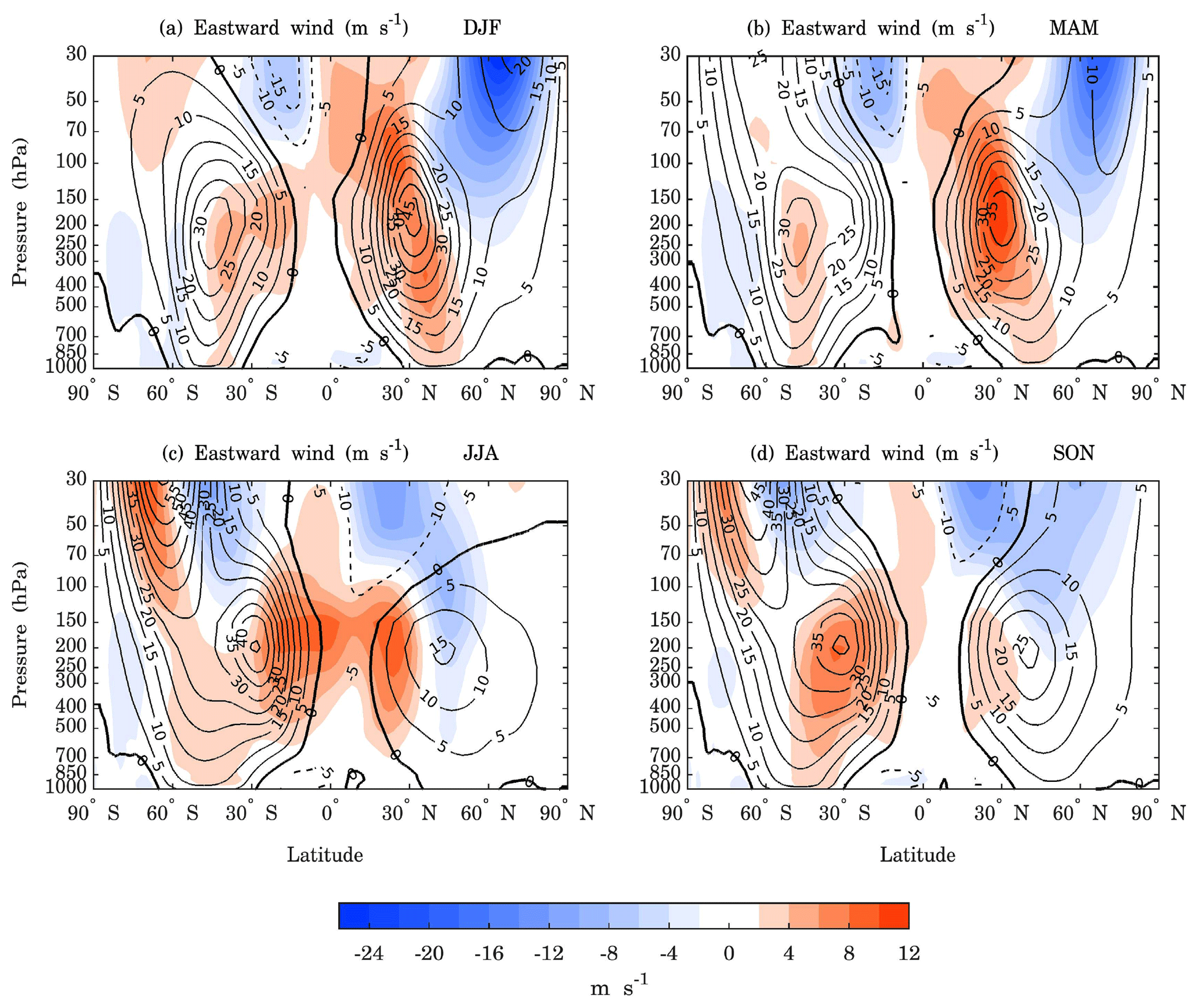
Figure 9 Contour lines showing the zonally averaged zonal wind for BESM-OA2.5 and the differences between the BESM-OA2.5 and 20CRv2 datasets are shaded. Both datasets were averaged over the period 1971–2000. The solid contour lines represent eastward zonal wind and the dashed contour lines represent westward zonal wind. The units are in meters per second and the contour interval is 5 m s⁻¹, with the zero-contour line highlighted.

Concerning the zonal wind, BESM-OA2.5 simulated a much weaker wind speed in the tropopause and stratosphere over the boreal hemisphere, mainly during the DJF season, which has a maximum negative bias of −26 m s⁻¹ at 50–30 hPa (Fig. 9a). This bias is out of the range (−10 to 10 m s⁻¹) presented by some other models, including NorESM1-M (Fig. 10; Bentsen et al., 2013) and NESMv3 (Fig. 10d; Cao et al., 2018). The tropospheric jets and their seasonal migration were reasonably well simulated, although the eastward wind was stronger in the subtropics, with a maximum positive bias of 12 m s⁻¹ at 300–100 hPa during the MAM season.

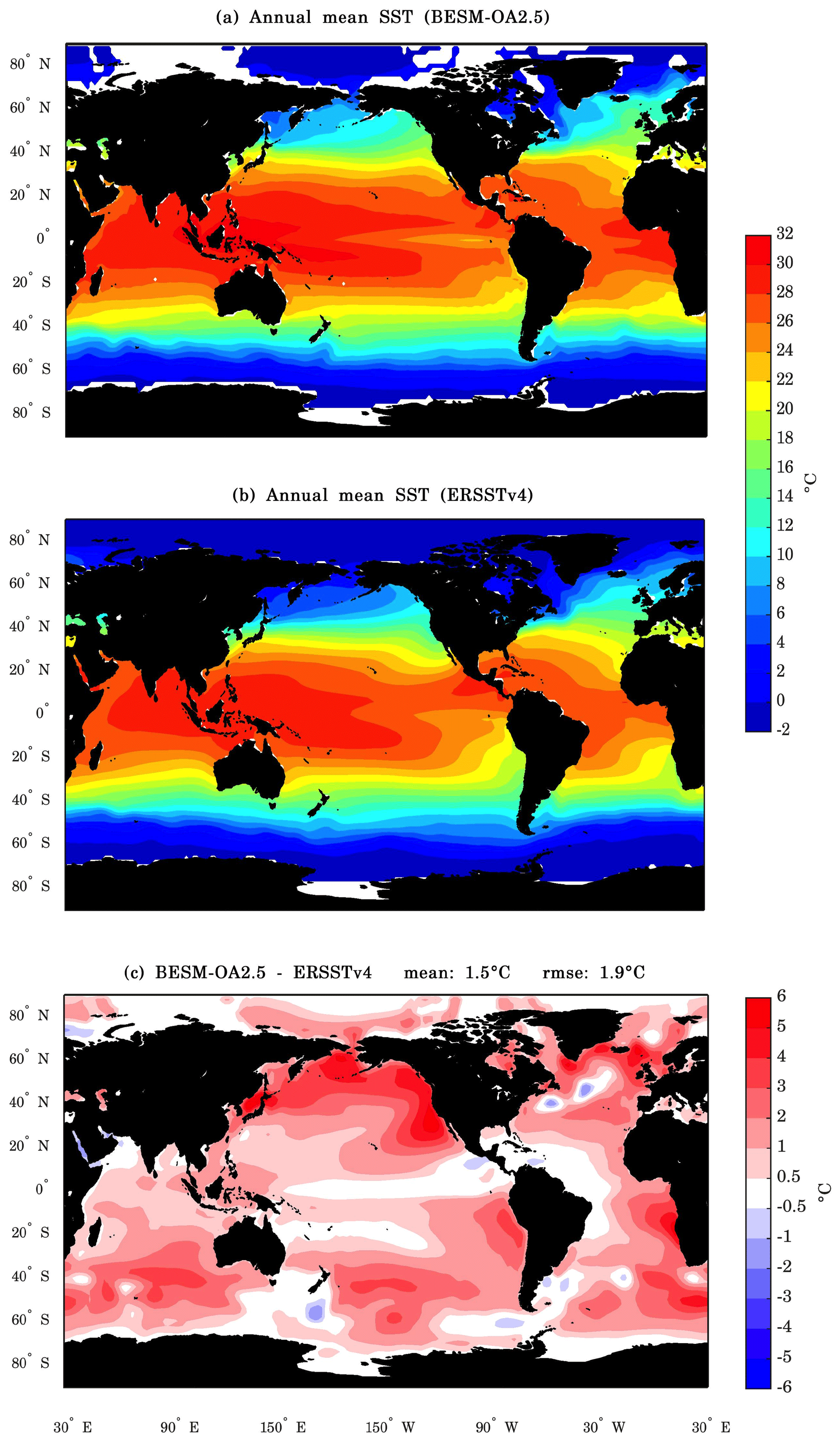
Figure 10 Spatial maps of the annual mean sea surface temperatures generated by (a) BESM-OA2.5 and (b) ERSSTv4, and (c) the bias of BESM-OA2.5 relative to ERSSTv4. The averages were computed over the period 1971–2000. Units are in degrees Celsius.

4.1.4 Ocean mean state

The global distribution and the range values of SST are important characteristics of the mean climate state. Figure 10 shows a spatial map of the annual mean SST values for (a) BESM-OA2.5 and (b) ERSSTv4 as well as (c) the bias for BESM-OA2.5 relative to the ERSSTv4 dataset. BESM-OA2.5 showed a warm SST bias that spread throughout all of the oceans, in contrast with the negative biases shown by most of the CMIP5 models over the North Pacific and North Atlantic oceans (see Wang et al., 2014). However, the extreme values found in the south of Greenland and in the North Pacific, where they reached ∼6 ^∘C, are well within the range of the biases reported by other models, including NorESM1-M (Fig. 12b; Bentsen et al., 2013) and IITM-ESM (Fig. 3; Swapna et al., 2018). Such warm biases do not appear in the tropical and subtropical regions in the BESM-OA2.3 simulation (Fig. 5a of Nobre et al., 2013), where there are instead cold SST biases. The spatial average biases are 1.5 and 0.9 ^∘C, and the RMSEs are 1.9 and 2.1 ^∘C for BESM-OA2.5 and BESM-OA2.3, respectively. A notable feature of BESM-OA2.5 is its strong warm SST bias in the North Pacific and off the California coast and south of Greenland. The model still overestimated the SSTs in the major eastern coastal upwelling regions. This feature is a systematic error observed in different state-of-the-art models that could be caused by the simulation of weaker-than-observed alongshore winds, which consequently leads to an underrepresentation of the upwelling and alongshore currents (e.g., Humboldt, California, and Benguela currents), and/or the underpredicted effects of shortwave radiation due to deficient simulation of stratocumulus clouds over cold waters (see Richter, 2015). Nevertheless, the bias was negligible over the north equatorial Pacific and in large parts of the tropical western Atlantic.

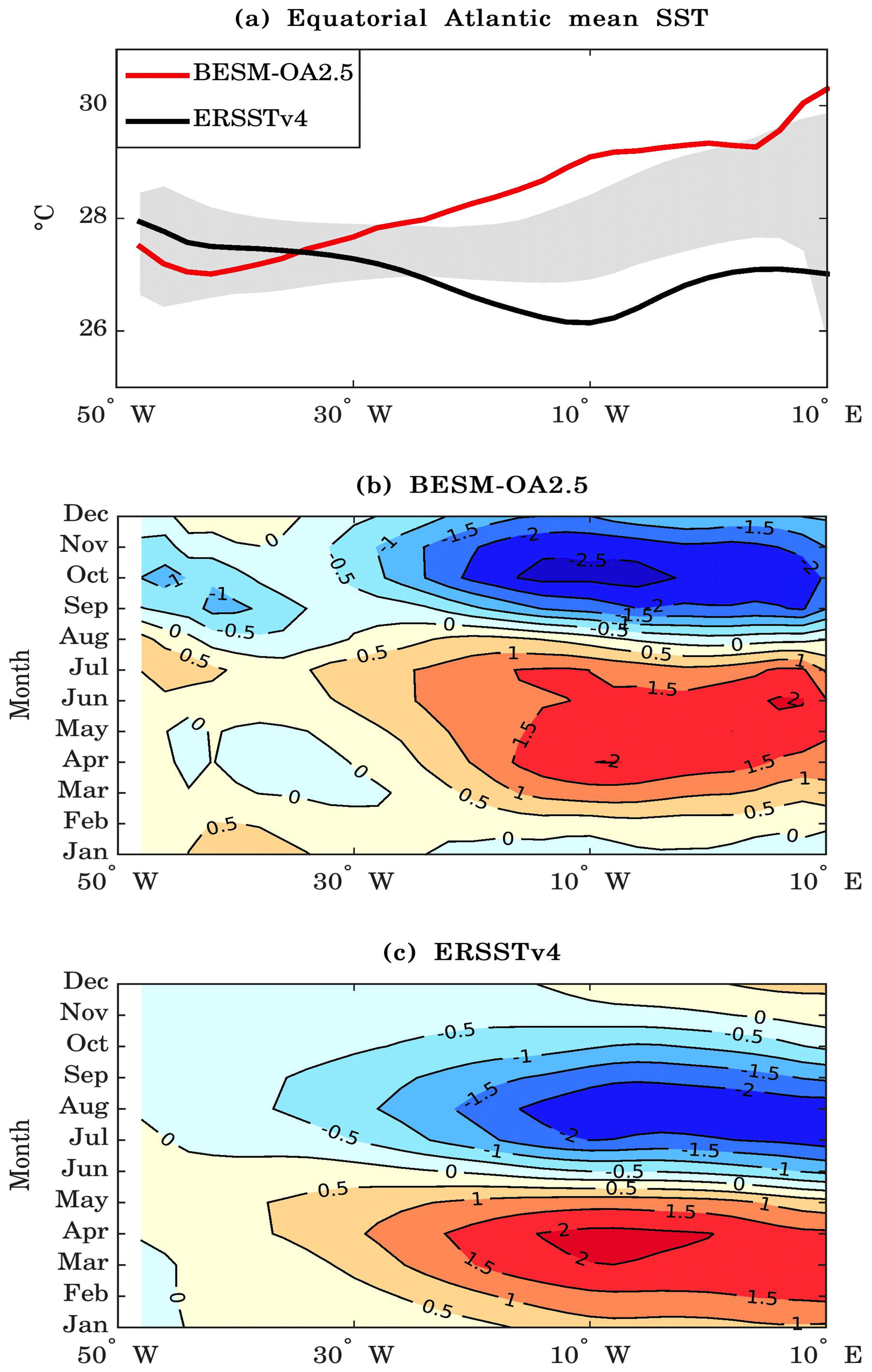
Figure 11a shows the mean SSTs in the equatorial Pacific for BESM-OA2.5 and ERSSTv4, averaged over the period 1971–2000. The equatorial region is defined as the region lying between the latitudes 2^∘ S and 2^∘ N. The model simulated a warmer mean SST over the western and extreme eastern parts of the equatorial Pacific Ocean. This positive bias was most notable in the western part of the Pacific, where it was about 1.5–2 ^∘C warmer than the observed values and was warmer than the values from the CMIP5 models (shown by the shaded grey area in Fig. 11a). However, for the extreme eastern part of the basin, the model showed a lower bias compared with those of the CMIP5 models. For most of the central Pacific Ocean, BESM-OA2.5 yielded a very good representation of the SSTs, with a RMSE of 0.14 ^∘C between 160^∘ E and 120^∘ W. The annual cycle of the equatorial Pacific SST anomalies for BESM-OA2.5 and ERSSTv4 are shown in Fig. 11b and c, respectively. BESM-OA2.5 simulated the marked annual cycle that occurs on the eastern Pacific reasonably well, although the negative SST anomalies between July and December are up to 1 ^∘C colder than the observed values. The propagation of the SST anomaly patterns from the eastern to the western parts of the Pacific Ocean that occurs throughout the year was not well captured by the model. BESM-OA2.5 showed an annual cycle in the western part of the Pacific Ocean, where the observations show a semiannual pattern of SST anomalies. The same methodology was used for the tropical Atlantic. Figure 12a shows that in the Atlantic basin there was a significant bias of about 3 ^∘C in the eastern part of the basin. This bias started in the central Atlantic and was higher than the biases of the CMIP5 models (shown by the shaded grey area in Fig. 12a). However, it should be noted that the CMIP5 models also have a warm bias in the eastern part of the tropical Atlantic, which is a problem discussed in previous studies (e.g., Richter et al., 2014, and references therein). Despite this warm bias, the tropical Atlantic seasonal SST variation was well simulated by BESM-OA2.5, in particular on the eastern side of the basin, as can be seen in Fig. 12b and c.

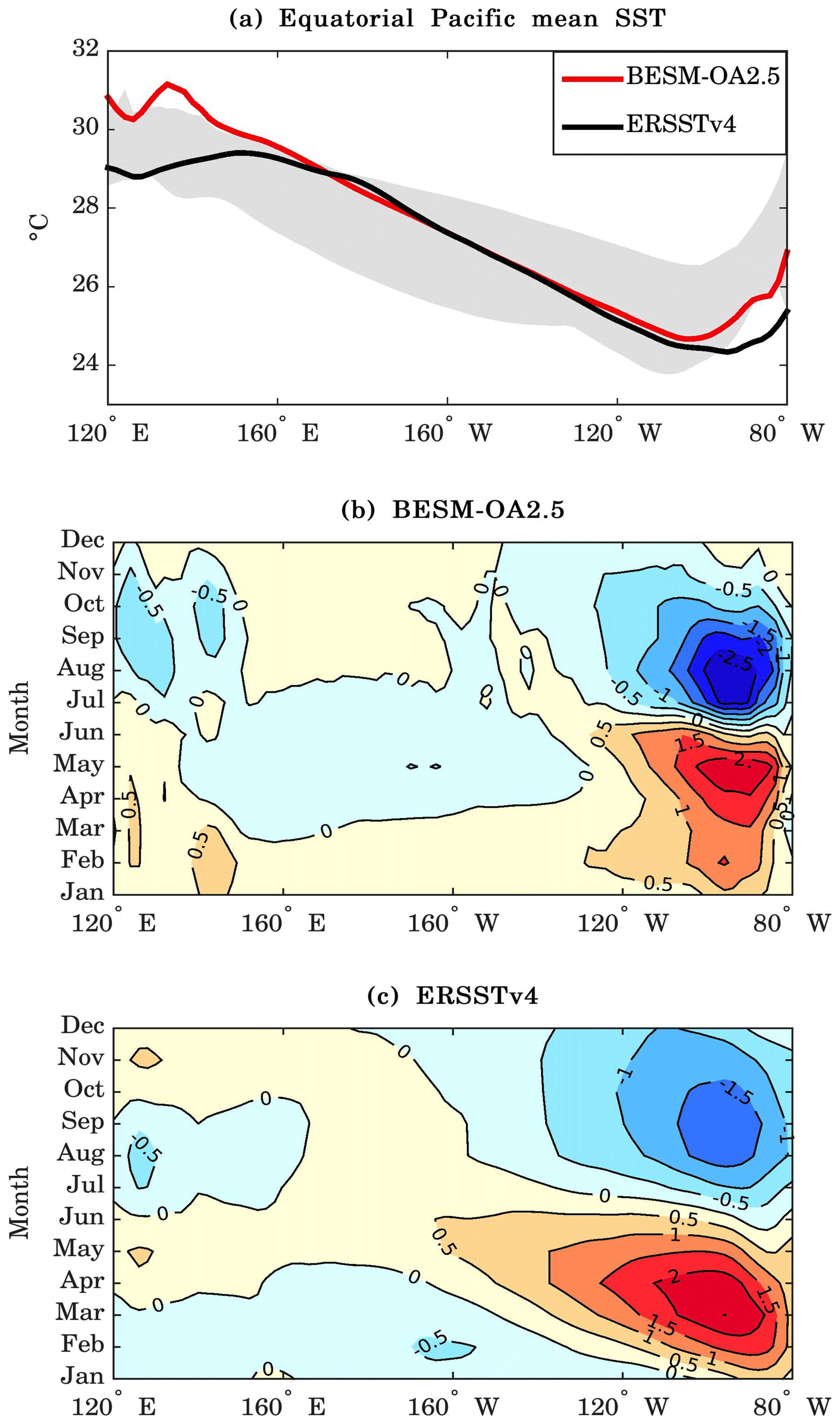
Figure 11 (a) Mean SSTs along the Equator in the Pacific Ocean and the annual cycle of the equatorial Pacific SST anomalies for (b) BESM-OA2.5 and (c) ERSSTv4. The equatorial region is defined by averaging over 2^∘ S–2^∘ N. The BESM-OA2.5 and ERSSTv4 data were averaged over the period 1971–2000. In (a), the grey shading represents the spread of 11 CMIP5 models, which were also averaged over the period 1971–2000. Units are in degrees Celsius.

Figure 12 As Fig. 11, but for the Atlantic Ocean.

To evaluate how the global ocean profile evolves throughout the simulation, depth–time Hovmöller diagrams of global mean ocean salinity and temperature departures from their respective initial conditions were calculated (Fig. 13a and b) in the historical simulation. Here, “initial condition” indicates the value of the first year of the simulation, in this case 1850. The ocean salinity slightly increased below a depth of 1000 m and from 1935 on, the increase reached 0.04 PSU between depths of 1500 and 3000 m compared with the initial values (Fig. 13a). Above a depth of 1000 m, there was a significant freshening of the ocean waters, with the surface water salinity decreasing up to 0.18 PSU by the end of the simulation. Concerning ocean temperature, prominent warming occurred from the surface up to a depth of 400 m (Fig. 13b). This warming was more significant at the end of the simulation (∼0.6 ^∘C compared with the initial conditions) and was mostly caused by the ocean warming drift in the model. Figure 13c shows the same diagram for a piControl simulation (during the period in which both simulations were performed in parallel), which also shows the ocean drift feature. However, the ocean temperature anomalies above 600 m reach approximately 0.6 ^∘C in the historical simulation, whereas they only reached approximately 0.4 ^∘C in the piControl. This difference of 0.2 ^∘C between the two simulations is likely due to the global warming of the planet and consequential increasing heat flux from the atmosphere into the ocean (Fig. 13d). In deeper waters, from 1500 m down to the ocean floor, there was weaker warming, indicating that the ocean is gaining heat mainly in its upper layers (Fig. 13b). Between the depths of 500–1500 m, a cooling tendency was observed relative to the initial conditions. Such a tendency could indicate that the ocean is still drifting from its initial conditions in the historical simulation.

Figure 13 Depth–time Hovmöller diagrams of the global average ocean (a) salinity and (b) temperature anomalies from the respective initial conditions (IC). Here, the initial conditions were taken from the first year for (a, b) historical simulation and from the 14th year for the (c) piControl simulation. The map shown in (d) presents the difference between the temperature anomalies of the historical simulation relative to the piControl. The diagrams are based on annual average time series simulated by the historical simulation over the period 1850–2005 (156 years) and by the piControl simulation over the period 14–169 years (156 years). The thick black line represents the zero contours. Note that the vertical scales are different above and below 1000 m.

The meridional overturning circulation (MOC) plays an important role in transporting heat from the tropics to the higher latitudes in both hemispheres. This is particularly important in the North Atlantic, where the Atlantic meridional overturning circulation (AMOC) has a profound impact on the climate of the surrounding continents (see Buckley and Marshall, 2016). The AMOC in the BESM-OA2.5 historical experiment showed the typical structure described in Lumpkin and Speer (2007): the upper layer of the upper cell, which is the northward flux, depicted at the appropriate depth, from the surface down to ∼1000 m (Fig. 14a). However, the upper cell simulated by BESM-OA2.5 was too shallow compared with the RAPID measurements (McCarthy et al., 2015). The depth of the upper cell was 2500 m in the model, whereas the measurements show its depth at ∼4500 m. This shallow upper cell of the AMOC is a common feature of state-of-the-art climate models (see Menary et al., 2018). In the deep ocean, the model accurately simulated the Antarctic Bottom Water flowing northwards over the Atlantic Ocean floor. The annual mean maximum AMOC strength simulated by BESM-OA2.5 is about 15 Sv (sverdrup, 1 Sv ≡ 10⁶ m³ s⁻¹) between 25 and 30^∘ N at a depth of about 850 m (Fig. 14a). This maximum value is within the 17.2±4.6 Sv mean strength (with a 10 d filtered root-mean-square variability of 4.6 Sv) observed at 26.5^∘ N by the RAPID project (McCarthy et al., 2015). This value is also in the range of the maximum volume transport strength simulated by other state-of-the-art CMIP5 models (Weaver et al., 2012; Cheng et al., 2013). Figure 14b shows the maximum annual mean AMOC strength time series for the historical period at 30^∘ N. For comparison, Fig. 14c shows the AMOC maximum volume transport strength measured by the RAPID project over the period April 2004 to October 2015 (http://www.rapid.ac.uk/rapidmoc/rapid_data/datadl.php, last access: 27 February 2019).

Figure 14 (a) The Atlantic Meridional Overturning Circulation averaged for the period 1971–2000 and (b) the annual mean maximum AMOC strength time series at latitude 30^∘ N simulated by BESM-OA2.5 for the historical simulation over the period 1850–2005. (c) The graph shows the AMOC time series measured by the RAPID project at 26.5^∘ N over the period April 2004 to October 2015. The RAPID time series is smoothed by a 3-month running average. Units are in sverdrup.

After averaging the maximum AMOC strength over the first and the last 30 years of the time series, i.e., over the periods 1850–1879 and 1976–2005, respectively, the result shows a decrease of 11.2 %, from 16.9 to 15.1 Sv during each period. Modeling results indicate that the AMOC has a multidecadal cycle; however, the power spectrum of its strength time series did not show a multidecadal oscillation (not shown). The standard deviation of the detrended maximum AMOC strength time series is 1.4 Sv.

Figure 15 shows the mean sea ice concentration simulated by BESM-OA2.5 for the end of the winter and the summer seasons for each hemisphere over the period 1971–2000. The thick black lines represent the 15 % climatological values for the period 1971–2000 given by the 20CRv2 reanalysis. The sea ice concentration at the end of the Arctic winter was overestimated in the Atlantic, specifically north of Scandinavia (Fig. 15a). However, at the end of the Arctic summer, the sea ice concentration was underestimated (Fig. 15b). At the end of the Antarctic summer, the model showed a significant underestimation of the sea ice concentration (Fig. 15c), whereas at the end of the Antarctic winter, the model generally overestimated the extension of the sea ice concentration over the Southern Ocean (Fig. 15d). Such seasonal sea ice concentration variations are likely related to the radiative net bias inherent in the model at high latitudes, which results in the generation of higher sea ice extensions during the winter season in each hemisphere compared with those from the reanalysis dataset and excessive sea ice melting during the summer season in each hemisphere.

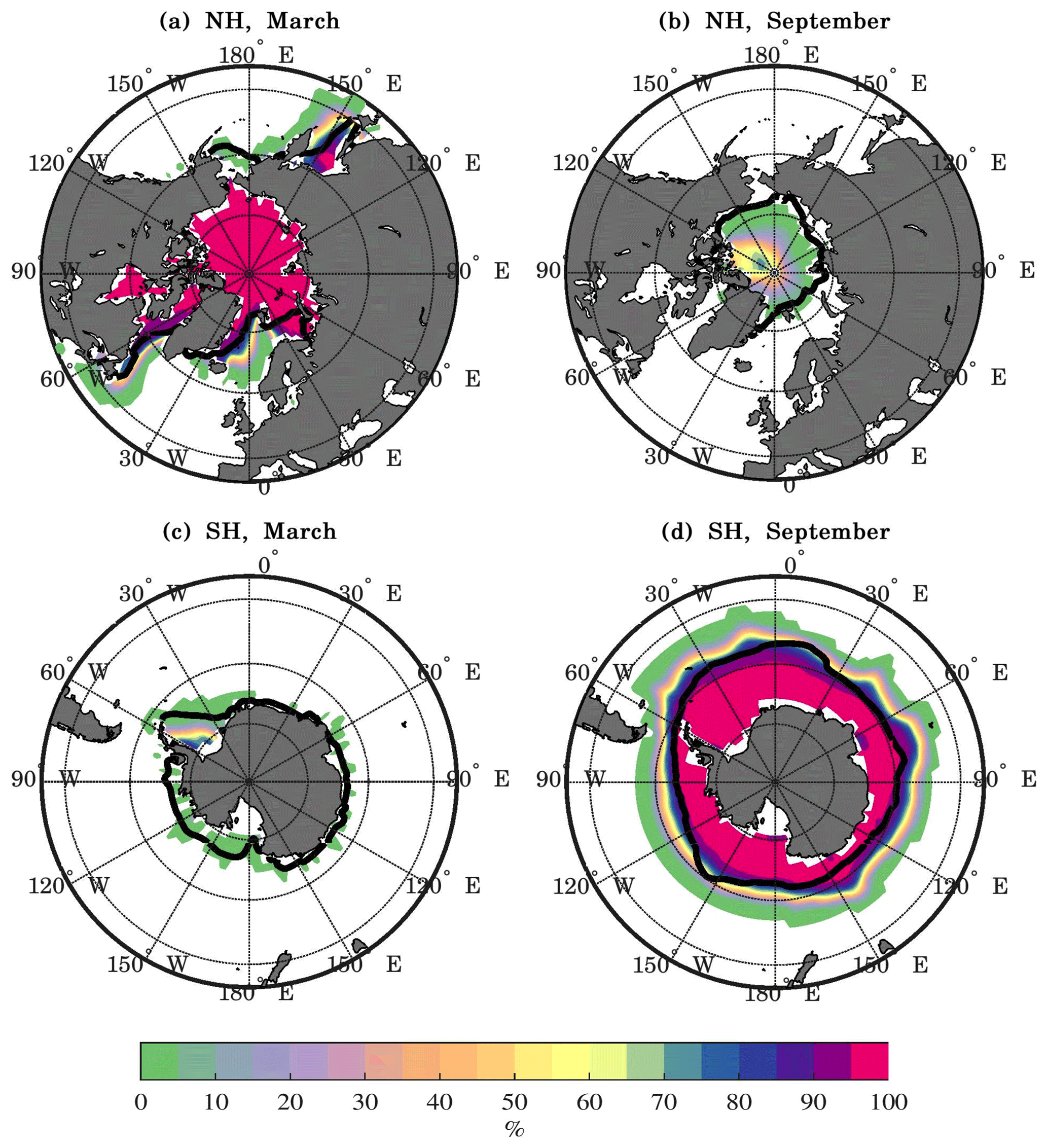
Figure 15 BESM-OA2.5 mean sea ice concentrations for March (a, c) and September (b, d) for each hemisphere. The solid black lines show the 15 % mean sea ice concentration from the 20CRv2 reanalysis. The average values were computed over the period 1971–2000 for BESM-OA2.5 and 20CRv2. The concentrations are presented as percentages.

4.2 Climate variability

In this section, we evaluate the most prominent global climate variability patterns. This evaluation allows us to understand the ability of the model to correctly simulate atmospheric internal and ocean–atmosphere coupled variabilities in the climate system.

4.2.1 Tropical variability

El Niño–Southern Oscillation

The El Niño–Southern Oscillation (ENSO) in the equatorial Pacific Ocean is one of the most prominent climate variability phenomena on interannual timescales (Dijkstra, 2006), and it has strong effects on regions surrounding the Indian Ocean and Pacific Ocean and regions that are influenced by its teleconnections (see McPhaden et al., 2006, and references therein). There are many methods to evaluate the ENSO variability. In the present study, the EOF was applied to detrended monthly SST anomalies over the tropical Pacific Ocean (30^∘ S–30^∘ N, 240–70^∘ W) for the period 1950–2005 for both the BESM-OA2.5 historical simulation and the ERSSTv4 data. Figure 16a and b show the leading EOF patterns associated with the El Niño/La Niña variability. The model was ineffective at simulating the El Niño/La Niña variability with lower amplitudes in the SST variability and with the center of maximal variability confined to the eastward part of the basin. The model's leading EOF explains 17.9 % of the total variance, substantially less than the 45 % explained by observations. The lower amplitude of the simulated El Niño/La Niña can be verified in the power spectrum of the leading PC shown in Fig. 16c and d. Even though the simulation shows two significant peaks between the 2–4 years cycle (Fig. 16c), which is within the range of the period cycle given by the leading PC of the observations (3–7 years cycle; Fig. 16d), the amplitude of the simulated variance is lower than that of the observations.

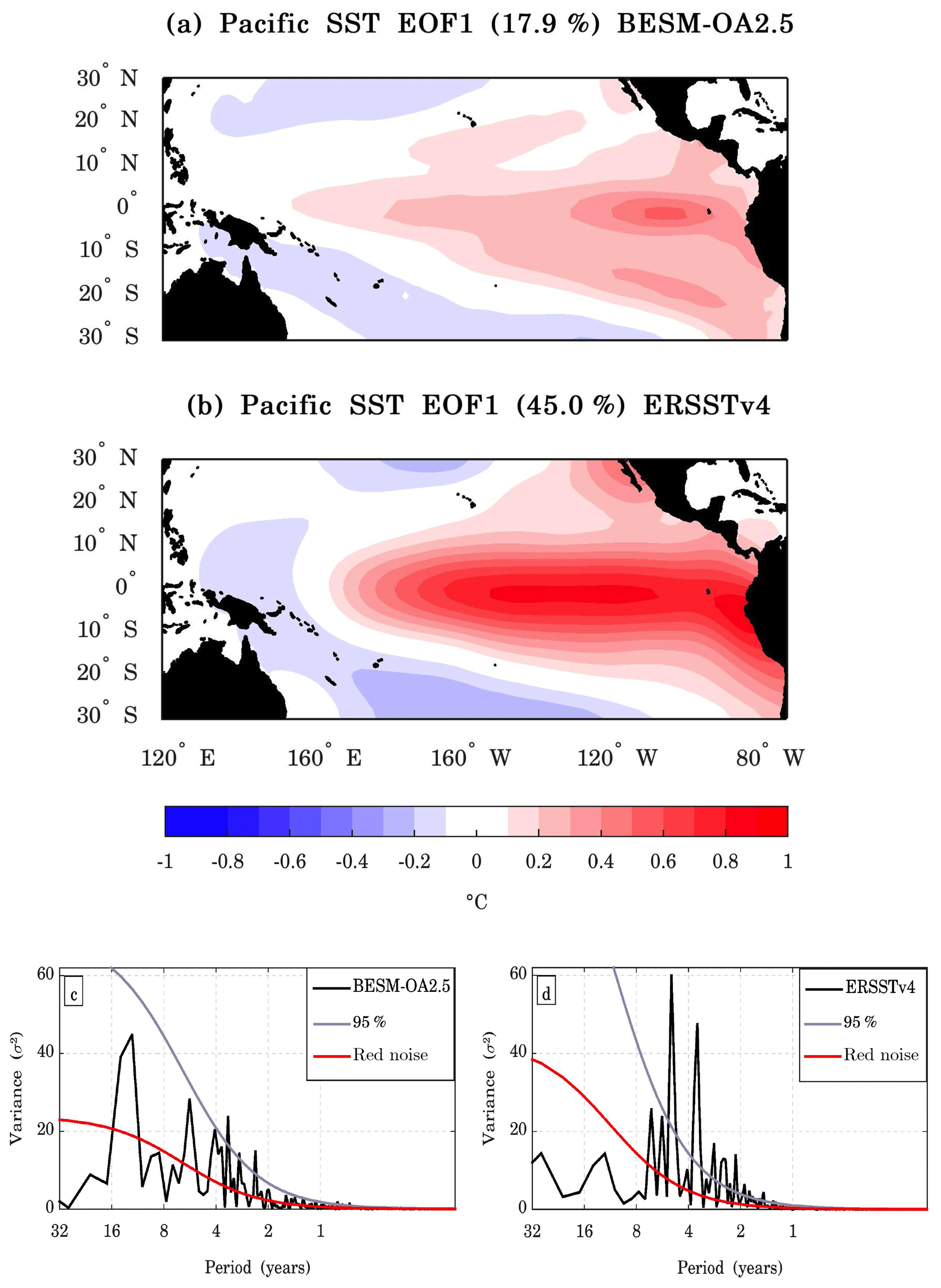
Figure 16 The leading EOF modes of the detrended monthly SST anomalies over the tropical Pacific region (30^∘ S–30^∘ N, 240–70^∘ W) for (a) BESM-OA2.5 and (b) ERSSTv4. The results are shown as the SST anomalies regressed onto the corresponding normalized PC time series (degrees Celsius per standard deviation) over the period 1950–2005. The percentages of the variance explained by each EOF are indicated in the titles of the panels. The contour interval is 0.1 ^∘C. Panels (c) and (d) show the power spectra of the leading joint PC time series of the patterns for BESM-OA2.5 and ERSSTv4, respectively. The solid red line represents the theoretical red noise spectrum and the gray line represents the 95 % confidence level.

Figure 17 shows the spatial correlation between the detrended monthly anomalies of the Niño-3 index (defined inside the black rectangular area, bounded by 5^∘ S–5^∘ N, 90–150^∘ W) and detrended monthly anomalies of global SSTs computed by BESM-OA2.5 and ERSSTv4 over the period 1900–2005. The model did not show a strong correlation at grid points inside the Niño-3 area, which is a signal that the El Niño/La Niña spatial pattern is weakly simulated. The horseshoe pattern of negative correlation observed over the Pacific Ocean is also weakly simulated by the model, particularly in the westward equatorial region. The positive correlation between the observed SSTs over the Indian Ocean and the Niño-3 index was absent in the model's simulation. It is worth mentioning that the model simulated the observed correlation pattern of SST anomalies over the Atlantic Ocean with the Ninõ-3 index, although it is not so robust (Fig. 17a).

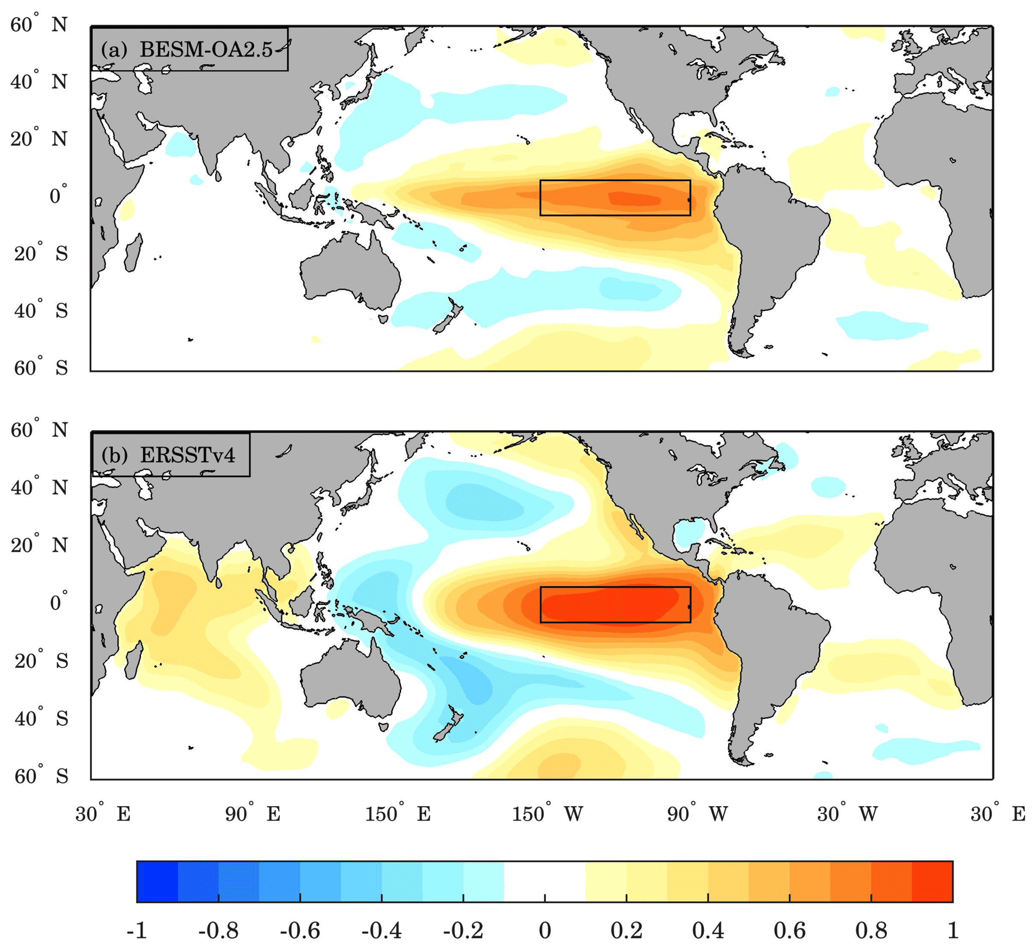
Figure 17 Spatial maps with the monthly correlations between the Niño-3 index and the global SST anomalies computed by (a) BESM-OA2.5 and (b) ERSSTv4 over the period 1900–2005. The anomalies were obtained by subtracting the monthly means for the entire detrended time series at each grid point. Black rectangles show the Niño-3 index region. Shaded areas are statistically significant at the 95 % confidence level (based on two-tailed Student's t tests).

Atlantic Meridional Mode

The leading modes of coupled ocean–atmosphere variability over the tropical Atlantic Ocean are the zonal mode, also referred to as the equatorial mode (Zebiak, 1993; Lutz et al., 2015), and the meridional mode, also referred to as the interhemispheric mode (Nobre and Shukla, 1996). The first is an ENSO-like phenomenon that emerges in the Gulf of Guinea mainly during the boreal summer and has a strong impact on west African precipitation (Zebiak, 1993; Lutz et al., 2015). The second is characterized by a cross-equatorial SST gradient associated with meridional wind stress toward the warmer SST anomalies. The maximal amplitude of the meridional mode occurs during the boreal spring and influences the precipitation in northeast Brazil and west Africa (Nobre and Shukla, 1996; Chang et al., 1997; Chiang and Vimont, 2004). The Atlantic Meridional Mode (AMM) has an interannual and decadal temporal scale of variability and results from a thermodynamic coupling between wind speed, the sea surface evaporation induced by the wind stress, and the SST, a mechanism known as wind–evaporation–SST feedback (WES feedback; Xie and Philander, 1994; Chang et al., 1997; Xie, 1999). To evaluate the AMM simulations, a joint EOF of SST and wind stress (Taux and Tauy) fields was computed, as such variability is intrinsic to the coupled ocean–atmospheric system. Figure 18 shows the AMM simulated by BESM-OA2.5 and that obtained via observed data. The AMM pattern simulated by the model is similar to that obtained from observations, regardless of the weaker gradient pole in the South Atlantic. Nevertheless, the variance explained by the model (10.7 %) is very close to the observed value (11.8 %). The patterns shown in Fig. 18 are defined as a positive phase of the AMM, with the interhemisphere cross-equatorial wind from the south to the north and with corresponding negative SST anomalies over the southern pole and positive SST anomalies over the northern pole (the negative phase of the AMM is the reverse pattern). Over the second half of the twentieth century, the AMM showed a predominant decadal periodicity of 11–13 years. Figure 18c and d show the power spectra of the PC of the AMM patterns simulated by the model and based on observed data, respectively. It is possible to see that the pattern simulated by BESM-OA2.5 shows, similar to that derived from the observed data, a predominant periodicity on decadal timescales.

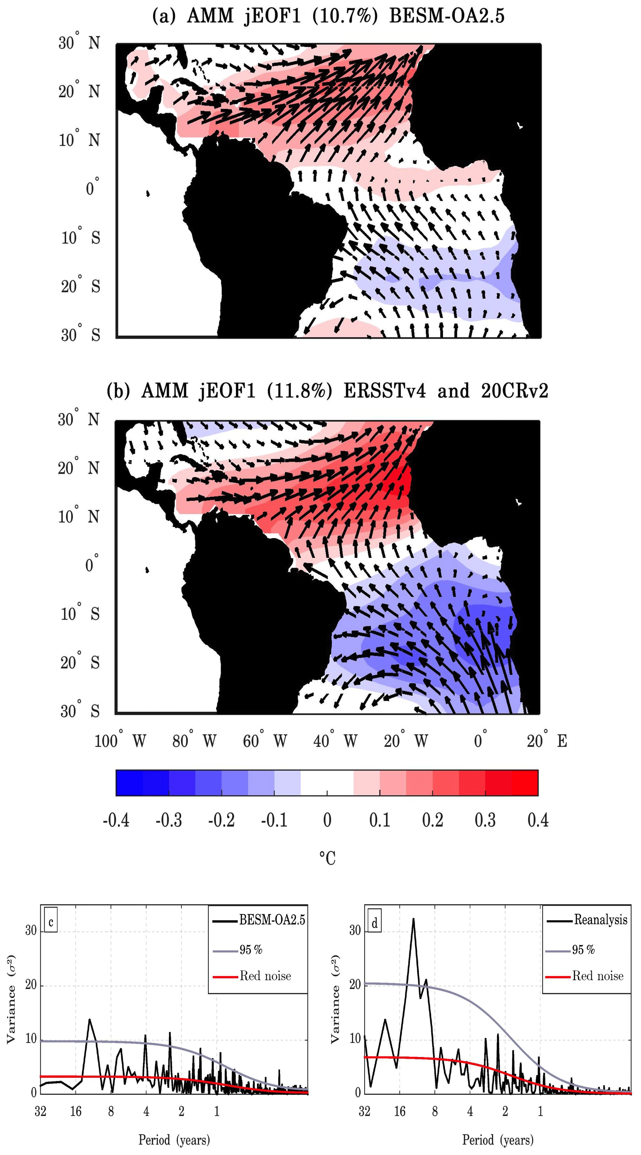
Figure 18 The leading joint EOF modes of the detrended monthly SST and wind stress (Taux and Tauy) anomalies for the tropical Atlantic region (30^∘ S–30^∘ N, 100^∘ W–20^∘ E) based on (a) BESM-OA2.5 and (b) from observation (ERSSTv4 and 20CRv2 reanalysis). The results are shown as the SST anomalies regressed onto the corresponding normalized PC time series (degrees Celsius per standard deviation) and wind stress anomalies regressed onto the corresponding normalized PC time series (meters per second per standard deviation) over the period 1950–2005. The percentages of the variance explained by each EOF are indicated in the titles of the figures. The contour interval is 0.05 ^∘C. Panels (c) and (d) show the power spectra of the leading joint PC time series of the AMM pattern simulated by BESM-OA2.5 and based on reanalysis, respectively. The solid red line represents the theoretical red noise spectrum and the gray line represents the 95 % confidence level.

South Atlantic Convergence Zone

The South Atlantic Convergence Zone (SACZ) is characterized by an intense NW–SE-oriented cloud band that extends from the Amazon Basin to the South Atlantic subtropics, mainly during the austral summer (Nogués-Paegle and Mo, 1997; Carvalho et al., 2004; de Oliveira Vieira et al., 2013). The formation of the SACZ has a strong influence on the precipitation over southeast South America and is considered, together with the convection activity over the Amazon Basin, the main component of the South American monsoon system (Jones and Carvalho, 2002). The southern part of the SACZ normally lies over cooler SSTs (Grimm, 2003; Robertson and Mechoso, 2000). Chaves and Nobre (2004) suggest that the cloud cover resulting from the formation of the SACZ over the ocean tends to block solar radiation, thus leading to cooler SSTs beneath. atmospheric general circulation models (AGCMs) are unable to simulate the precipitation over the cooler SSTs caused by the SACZ (Marengo et al., 2003; Nobre et al., 2006, 2012) since such models tend to increase the precipitation over warmer SSTs as a hydrostatic response. Nobre et al. (2012) showed that coupled atmosphere–ocean general circulation models (AOGCMs) can simulate SACZ formation over colder SST anomalies, as this class of models incorporates atmosphere–ocean surface thermodynamic coupling. Following Nobre et al. (2012), a correlation exists between the seasonal precipitation and SST anomalies during the austral summer (DJF) over the tropical South Atlantic (40^∘ S–10^∘ N, 70^∘ W–20^∘ E) over the period 1979–2010 for observations and over the period 1971–2002 for the model; therefore, 32 years were used. Figure 19 shows the rainfall–SST anomaly correlation maps for both BESM-OA2.5 and the observations. BESM-OA2.5 could simulate an inverse correlation between the precipitation and SST in the southeast of Brazil (near 20^∘ S), indicating it's capacity to simulate precipitation over cooler SSTs, a feature related to the formation of SACZ (which results in cooler SSTs). Its noteworthy in Fig. 19 that BESM-OA2.5 could generate both positive and negative sea surface temperature anomaly and rainfall correlations over the equatorial Atlantic (positive, thermally direct driven circulation over the equatorial region, and negative, thermally indirect driven atmospheric circulation over the SW tropical Atlantic, Fig. 19a), a feature also present in the observation correlation map shown in Fig. 19b.

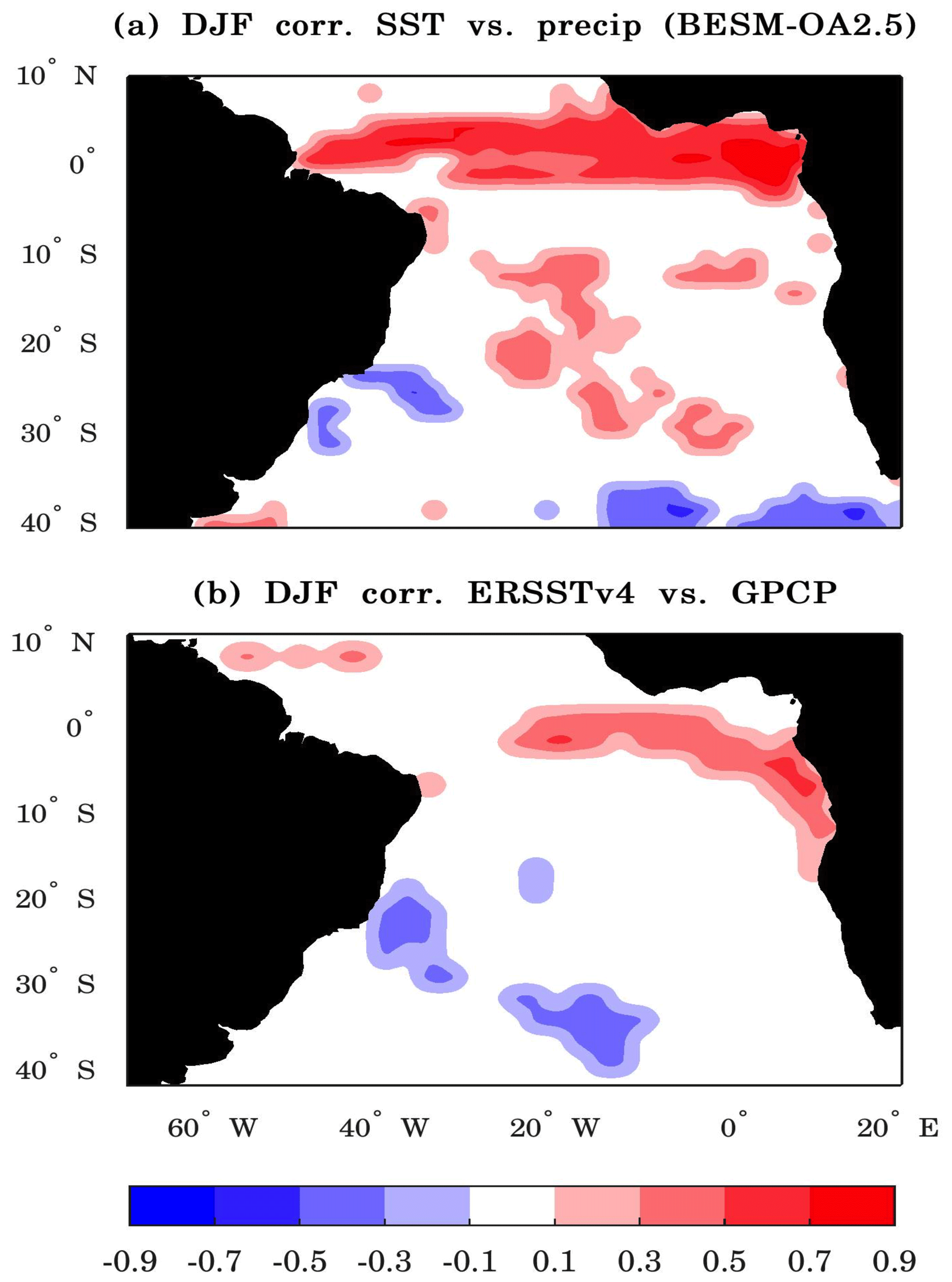
Figure 19 Spatial maps with the correlation between SST and precipitation (seasonal average DJF) over the South Atlantic Ocean (40^∘ S–10^∘ N, 70^∘ W–20^∘ E) computed by (a) BESM-OA2.5 over the period 1971–2002 and (b) based on reanalysis over the period 1979–2010. Shaded areas are statistically significant at the 95 % confidence level (based on two-tailed Student's t tests).

Madden–Julian oscillation

The Madden–Julian oscillation (MJO) is the primary intraseasonal variability (30–90 d) over the eastern Indian Ocean and western Pacific tropical regions and consists of deep convection events coupled to atmospheric circulation that propagate together eastward through the equatorial region (Madden and Julian, 1971, 1972; Zhang, 2005). The influence of MJO events on large-scale phenomena has been reported, as in the case of the evolution of ENSO (e.g., Takayabu et al., 1999), with the formation of tropical cyclones (e.g., Liebmann et al., 1994) and in the North Atlantic Oscillation (e.g., Lin et al., 2009). To evaluate the MJO simulated by the model, wavenumber–frequency power spectrum analyses were performed for tropical (10^∘ S–10^∘ N) averaged daily outgoing longwave radiation (OLR) and for the daily zonal wind component at the 850 hPa pressure level (U850) during the boreal winter (November–April) over the period 1971–2000. To compute and plot the wavenumber–frequency power spectra the MJO Simulation Diagnostic package was used (details in Waliser et al., 2009).

Figure 20a and b show the wavenumber–frequency power spectra for the OLR from BESM-OA2.5 and 20CRv2, respectively. Although BESM-OA2.5 yielded an eastward-propagating disturbance with wavenumber 1, it was characterized by a lower frequency (>80 d) compared to the maximal peak within the 30–80 d frequency band shown by the 20CRv2 data, despite its spread over frequencies less than 80 d. This observed peak has more energy for wavenumber 2. A westward-propagating disturbance (negative frequencies) with weaker energy than the eastward-propagating counterpart appears in the 20CRv2 datasets, with a peak for wavenumber 2. Similarly, BESM-OA2.5 also showed a westward-propagating disturbance with weaker energy for wavenumbers 1–3. The wavenumber–frequency power spectrum for U850 in 20CRv2 showed an eastward-propagating disturbance that peaked at the 30–80 d frequency band with wavenumber 1 (Fig. 20d). In the case of BESM-OA2.5, there was an eastward propagation with a periodicity slightly higher than 80 d for wavenumber 1, but this disturbance spread over different frequencies outside of the 30–80 d frequency band (Fig. 20c). BESM-OA2.5 also presented a westward-propagating disturbance that is absent in the reanalysis. BESM-OA2.5 poorly simulated the MJO and underestimated its amplitude. However, the MJO has been highlighted as a phenomenon that climate models struggle to properly simulate, especially via underestimation of the OLR and representation of a coherent eastward propagation (Kim et al., 2009; Ahn et al., 2017).

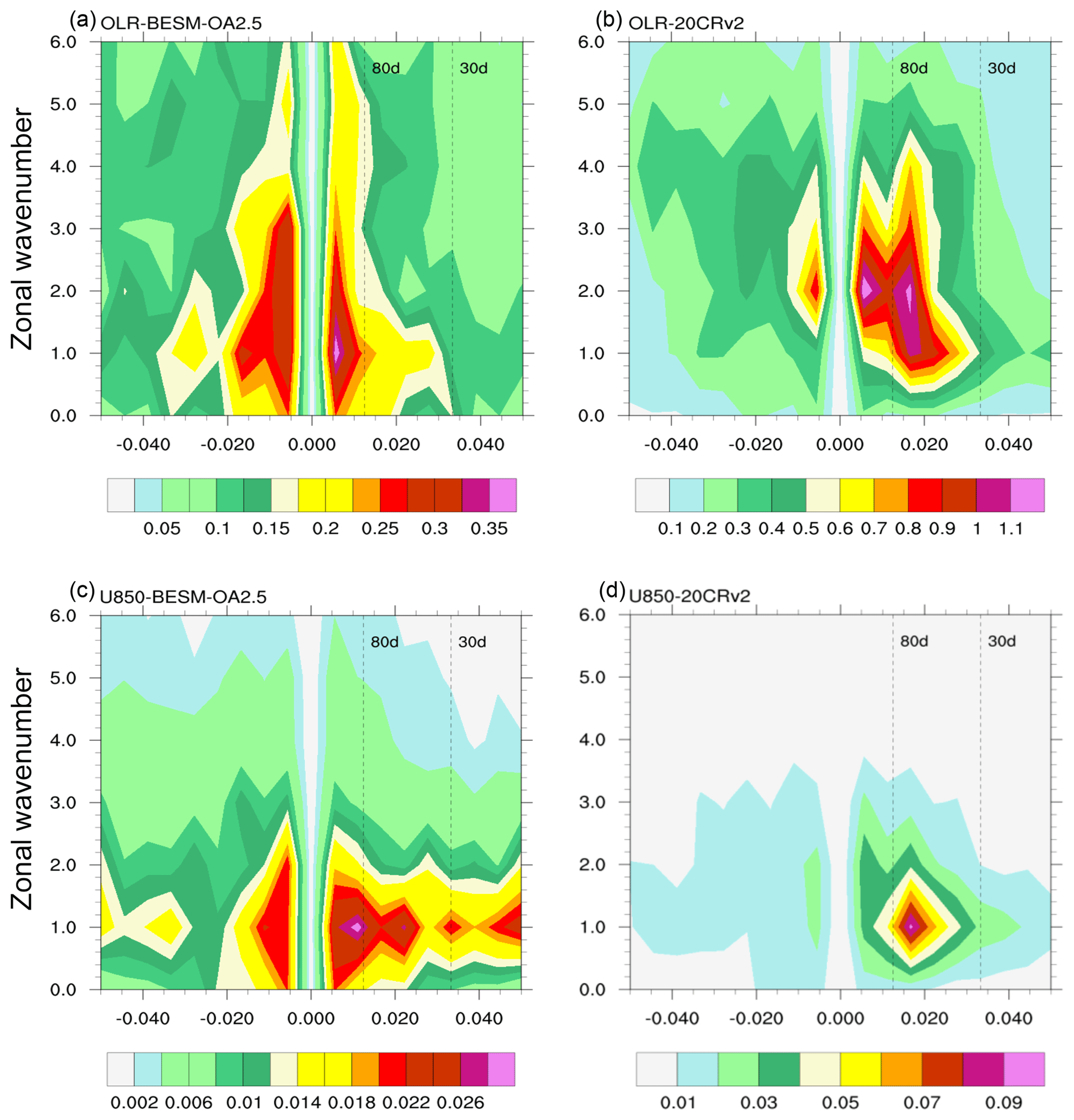
Figure 20 Wavenumber–frequency power spectra of the tropical (10^∘ S–10^∘ N) averaged daily outgoing longwave radiation (OLR) for (a) BESM-OA2.5 and (b) 20CRv2, and the averaged daily zonal wind component at 850 hPa pressure level (U850) for (c) BESM-OA2.5 and (d) 20CRv2. The data used were the daily anomalies for the boreal winter (November–April) over the period 1971–2000. The daily anomalies were obtained by subtracting the climatological daily mean calculated over the period 1971–2000. Individual spectra were calculated for each boreal winter and then averaged over the time period used. Units for the zonal wind ( and OLR) are m⁻² s⁻² (and W m⁻² s⁻¹) per frequency interval per wavenumber interval.

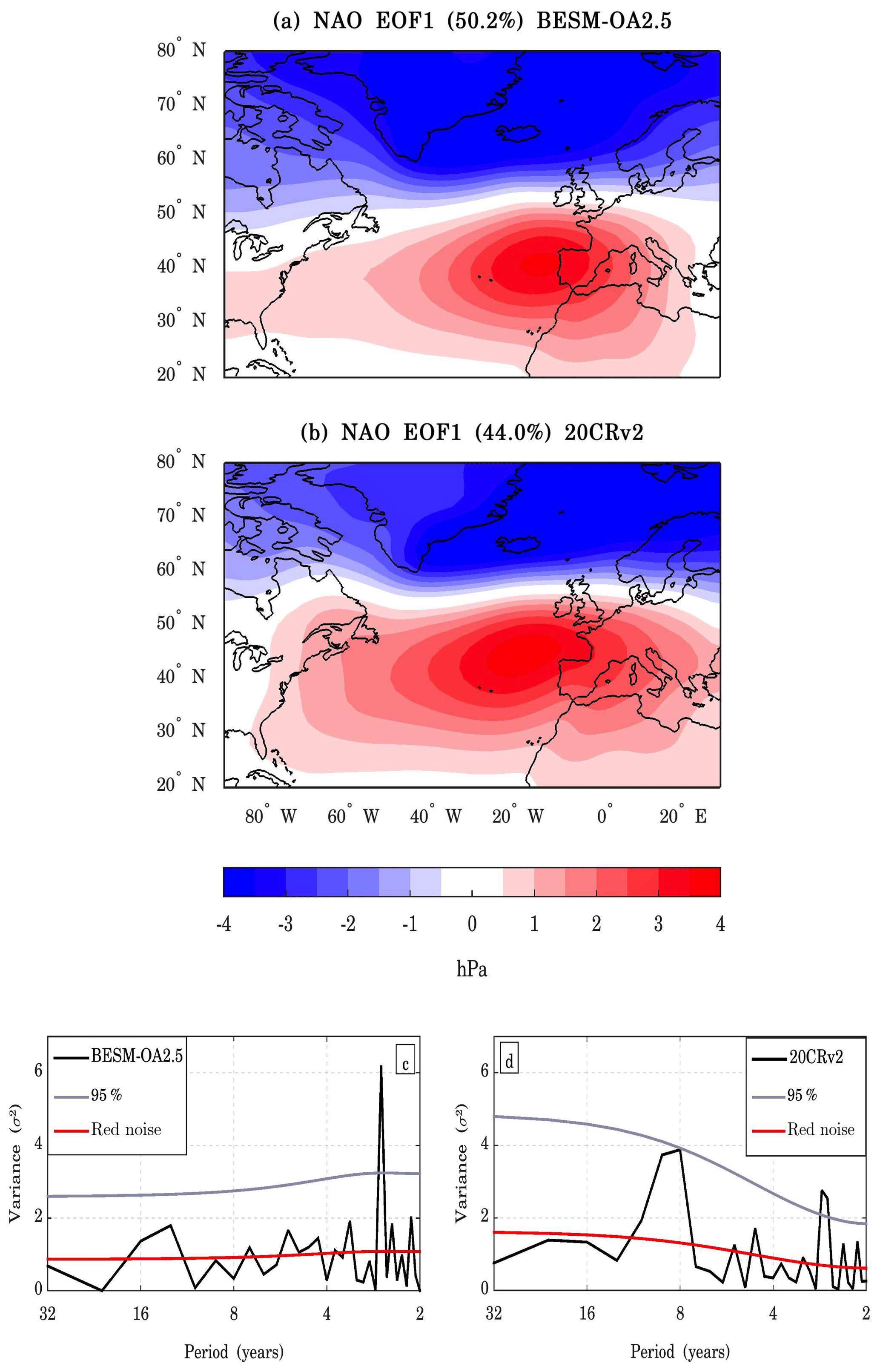
Figure 21 The leading EOF modes of the boreal winter (DJF) seasonal averaged sea level pressure (SLP) anomalies for the Euro-Atlantic region (20–80^∘ N, 100^∘ W–30^∘ E) for (a) BESM-OA2.5 and (b) 20CRv2. The results are shown as the SLP anomalies regressed onto the corresponding normalized PC time series (hectopascal per standard deviation) for the period 1950–2005. The percentages of the variance explained by each EOF are indicated in the titles of the figures. The contour interval is 0.5 hPa. Panels (c) and (d) show the power spectra of the leading PC time series of the North Atlantic Oscillation (NAO) pattern for BESM-OA2.5 and 20CRv2 reanalysis, respectively. The solid red line represents the theoretical red noise spectrum and the gray line represents the 95 % confidence level.

4.2.2 Extratropical variability

North Atlantic Oscillation

The North Atlantic Oscillation (NAO) is a major atmospheric variability pattern that occurs in the North Atlantic that is characterized by oscillations in the sea level pressure (SLP) differences between Iceland and Portugal (Wanner et al., 2001; Hurrel et al., 2003). The NAO has a robust impact in the Euro-Atlantic region (Hurrell et al., 2003; Hurrell and Deser, 2009), and the notable work of Namias (1972) connected the droughts in northeast Brazil to NAO variations. Recent studies show that it has teleconnections to East Asia (e.g., Yu and Zhou, 2004; Wu et al., 2012). The NAO's influence on rapid climate changes in the Northern Hemisphere has been highlighted in Delworth et al. (2016), thus making its correct simulation more critical. Since the NAO's largest amplitude of variation occurs mainly during the boreal winter, the analyses presented here are centered on this season, and the period used to perform these analyses was 1950–2005. The leading EOF of the SLP averaged over the boreal winter season (DJF) in the Euro-Atlantic region showed that the NAO is well simulated by BESM-OA2.5 (Fig. 21a), as its simulations of the NAO dipole centers and their amplitudes were very similar to the observed pattern (Fig. 21b). The variances explained by the leading EOF were also similar, 50.2 % and 44 % for BESM-OA2.5 and the 20CRv2 reanalysis, respectively. The spectral analysis of the leading PCs showed that BESM-OA2.5 captures the ∼2.5-year cycle in the time variability, but failed to capture the ∼8-year cycle (Fig. 21c and d). It is interesting to note that BESM-OA2.5 simulated a NAO spatial pattern without capturing its low-frequency variability. Based on an analysis of the NAO variability, we propose that it is not necessary to analyze the Northern Annular Mode (NAM), since both are manifestations of same mode of variability (Hurrell and Deser, 2009).

Pacific–North America pattern

Together, the NAO and the Pacific–North American pattern (PNA) are the dominant atmospheric internal modes over the boreal hemisphere. The PNA is characterized by four centers of the 500 hPa geopotential height anomalies in the North Pacific and over North America: centers located over Hawaii, in the south of the Aleutian Islands, in the intermountain region of North America, and in the Gulf Coast region of the USA, representing the centers of action of a stationary wave train extending from the tropical Pacific into North America (Wallace and Gutzler, 1981). The PNA exerts a significant influence on surface temperature and precipitation over North America (Leathers et al., 1991). Some studies have shown that although the PNA is an internal atmospheric variability phenomenon, it is influenced by other climate variabilities, including the ENSO and the Pacific Decadal Oscillation (PDO; see Straus and Shukla, 2002; Yu and Zwiers, 2007).

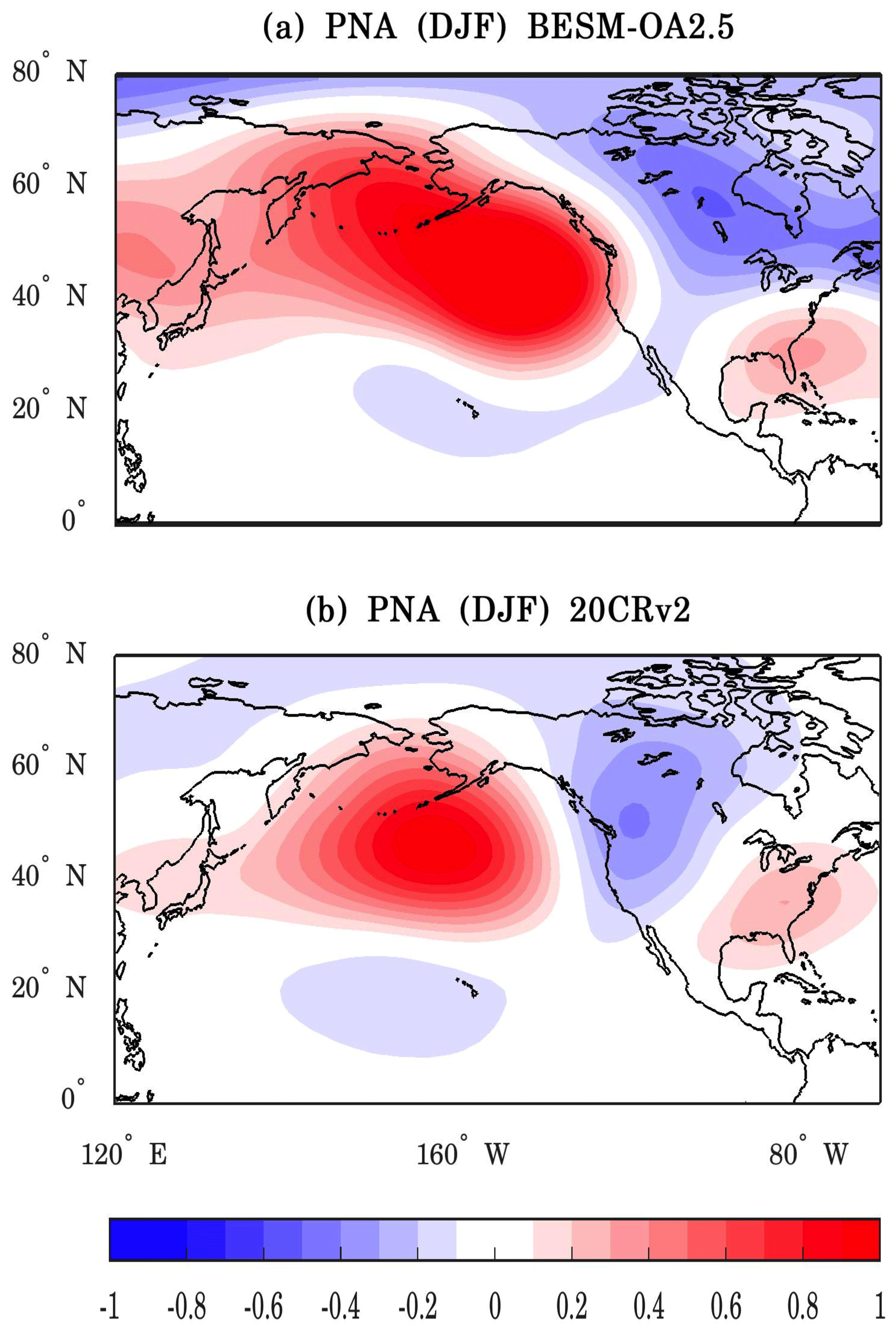
Figure 22 One-point correlation maps for (a) BESM-OA2.5 and (b) 20CRv2 reanalysis showing the correlation coefficient of 500 hPa geopotential height based at 45^∘ N, 165^∘ W and the other grid points. The time series used were from the boreal winter seasonal (DJF) averaged dataset for the period 1950–2005.

Similar to the NAO, the PNA has its largest variation in amplitude during the boreal winter; therefore, the present analyses were performed for this season. Following Wallace and Gutzler (1981), we constructed one-point correlation maps for BESM-OA2.5 and the 20CRv2 reanalysis to evaluate the capacity of the model to reproduce the PNA pattern. The one-point correlation maps correlate the 500 hPa geopotential height at the reference point (45^∘ N, 165^∘ W) with all of the other grid points on the map domain (0–80^∘ N, 240–70^∘ W). The time series used to perform the correlations were an averaged boreal winter seasonal (DJF) dataset over the period 1950–2005. The time series were departed from their long-term means and normalized at each grid point prior to the correlation computation. Figure 22 shows the one-point correlation maps for BESM-OA2.5 (Fig. 22a) and 20CRv2 (Fig. 22b). In that figure, it is possible to observe the four geopotential height centers simulated by the model, which show a stronger correlation when compared with the reanalysis correlation maps shown in Fig. 22b.

Pacific–South America patterns

The second and third EOF of the 500 hPa geopotential height over the Southern Hemisphere (20–90^∘ S) shares a notable resemblance to the Pacific–South America (PSA) teleconnection pattern (Mo and Peagle, 2001). PSA patterns are stationary Rossby wave trains that extend from the central Pacific to Argentina, in which the PSA1 (EOF2) is a response to the ENSO and the PSA2 (EOF3) is associated with the quasi-biennial component of the ENSO (Karoly, 1989; Mo and Peagle, 2001). These patterns have a significant impact on rainfall anomalies over South America (Mo and Peagle, 2001). Figure 23 shows the PSA patterns simulated by BESM-OA2.5 and from the 20CRv2 reanalysis. As the explained variance of EOF2 and EOF3 are similar, the EOFs seem to be degenerate for both the reanalysis and the model simulation. To relax the orthogonality constraint, a rotated EOF (REOF) retaining the first 10 modes was performed. REOF2 and REOF3 resembled EOF2 and EOF3, respectively, implying that they are independent modes. The PSA pattern was well simulated by BESM-OA2.5, although the model changed the order of the EOF patterns. BESM-OA2.5 showed an anomaly south of South Africa (Fig. 23c) that does not appear in the reanalysis (Fig. 23b). PSA patterns have significant interannual and decadal variabilities (Zhang et al., 2016). The PSA patterns simulated by BESM-OA2.5 had significant variability only on the interannual scale, with no decadal variability (figure not shown).

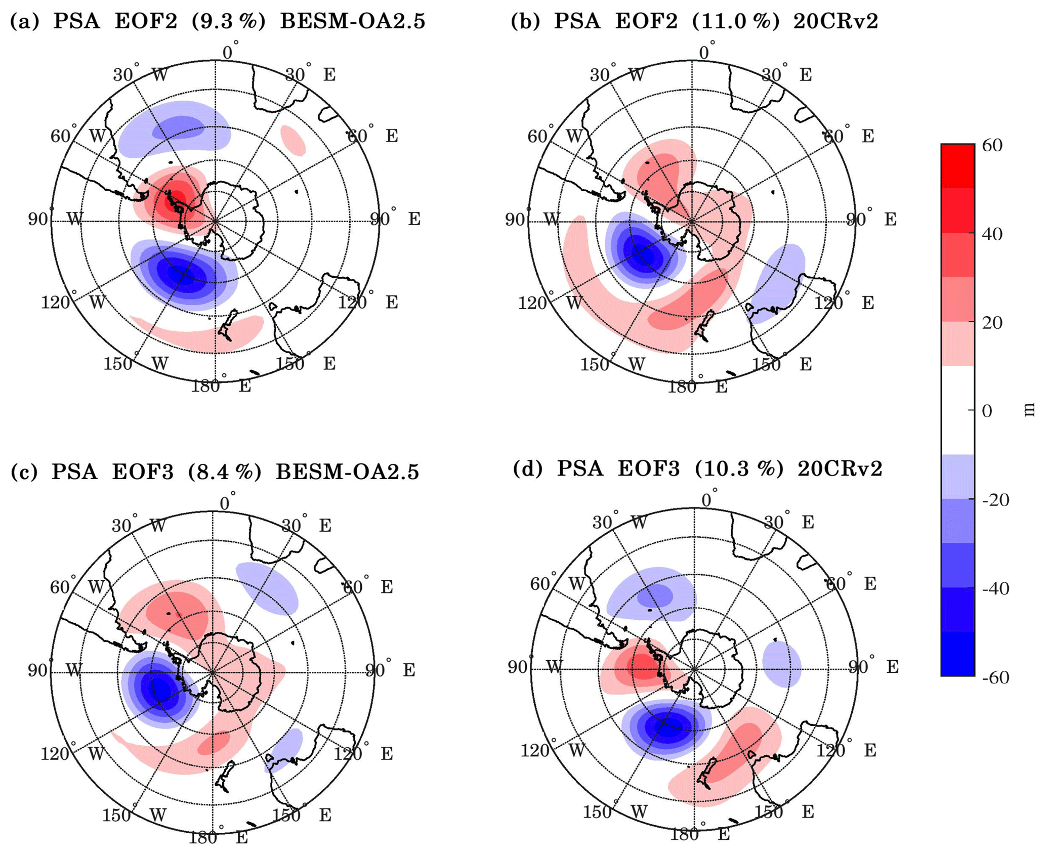
Figure 23 (a) The second and third EOF modes of the monthly mean 500 hPa geopotential height field for the Southern Hemisphere (20–90^∘ S) for BESM-OA2.5 (b) and 20CRv2 reanalysis. The results are shown as the 500 hPa geopotential height regressed onto the corresponding normalized PC time series (meters per standard deviation) over the period 1950–2005. The percentages of the variance explained by each EOF are indicated in the titles of the figures. The contour interval is 10 m.

Southern Annular Mode

The Southern Annular Mode (SAM) is the dominant atmospheric variability in the Southern Hemisphere, and it occurs in the extratropics and in the high latitudes (Kidson, 1988). It is also referred to as the Antarctic Oscillation (AAO; Gong and Wang, 1999). SAM variability is characterized by anomalous variations in the polar low pressure and in the surrounding zonally high-pressure belt. The SAM can be captured via the first EOF applied to different atmospheric variables, such as the sea level pressure, different geopotential height levels, and the surface air temperature (Kidson, 1988; Rogers and van Loon, 1982; Thompson and Wallace, 2000). To evaluate the capacity of BESM-OA2.5 to simulate this atmospheric mode of variability, EOF analysis was applied to the monthly mean 500 hPa geopotential height field from 20 to 90^∘ S over the period 1950–2005, for both the model and reanalysis. The SAM pattern simulated by BESM-OA2.5 strongly resembled the observed pattern, showing midlatitude 500 hPa geopotential height variation centers at the same longitudes as those observed, although it showed differences in the amplitude values (Fig. 24). However, the explained variance is higher compared with the observation. The explained variances of BESM-OA2.5 and 20CRv2 are 34.1 % and 21.0 %, respectively. The SAM is a quasi-decadal mode of variability (see Yuan and Yonekura, 2011); however, the BESM-OA2.5 power spectrum reveals a SAM with a markedly interannual variability, without the peak between 8 and 16 years contained in the reanalysis (figure not shown).

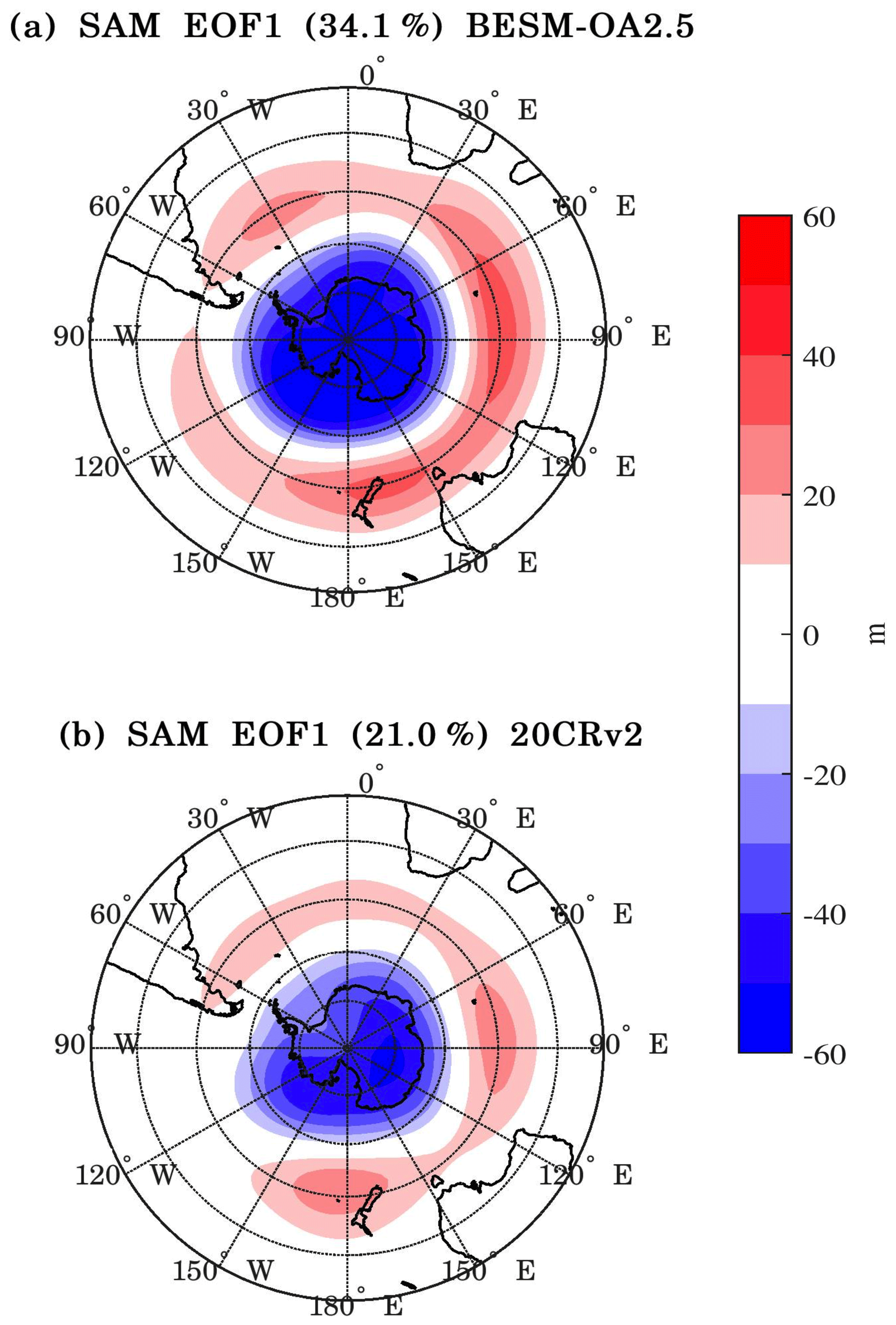
Figure 24 The leading EOF modes of the monthly mean 500 hPa geopotential height field for the Southern Hemisphere (20–90^∘ S) for (a) BESM-OA2.5 and (b) 20CRv2 reanalysis. The results are shown as the 500 hPa geopotential height regressed onto the corresponding normalized PC time series (meters per standard deviation) over the period 1950–2005. The percentages of the variance explained by each EOF are indicated in the titles of the figures. The contour interval is 10 m.

Pacific Decadal Oscillation

The observed SST anomalies over the North Pacific have shown an oscillatory pattern in the central and western parts in relation to the tropical part and along the North American west coast. This oscillatory shift in SST anomalies with interdecadal periodicity was termed the Pacific Decadal Oscillation (PDO), and it is defined as the leading EOF of the monthly SST anomalies over the North Pacific (Mantua et al., 1997). The positive phase of the PDO is defined when negative SST anomalies are predominate over the central and western parts of North Pacific and positive SST anomalies predominate over the tropical Pacific and along the North American west coast. The negative phase is a reversal of this pattern. Many studies have connected the PDO with variations in precipitation regimes in different regions around the world, including the South China monsoon (e.g., Wu and Mao, 2016), the Indian monsoon (e.g., Krishnamurthy and Krishnamurthy, 2016), and, together with the ENSO, the precipitation regime in North America (see Hu and Huang, 2009). There are different mechanisms that modulate the PDO, among which is the response of the Northern Pacific SST to the ENSO variability via the “atmospheric bridge” (for a detailed review, see Newman et al., 2016).

Following its definition (Mantua et al., 1997), the spatial pattern of the PDO was obtained by regressing the SST anomalies onto the leading normalized PC time series, as shown in Fig. 25, which in this case shows the positive phase of the PDO. The EOF was applied to monthly SST anomalies over the North Pacific (20–60^∘ N, 240–110^∘ W) over the period 1900–2005. BESM-OA2.5 was not capable of reproducing this pattern in the leading EOF. The PDO pattern only appeared on the second EOF (Fig. 25a) with an explained variance of 14.0 % compared with 20.5 % for the observations. Although the EOF2 resembles the PDO mode, the tropical part has weaker variation compared with the observed variation. The basis for the model's deficiency in reproducing the PDO as the leading mode of variability is probably the model's simulation of weaker ENSO variability, both on spatial and temporal scales. These deficiencies may impact the mechanisms that reproduce the PDO, mainly via the “atmospheric bridge” referred to earlier. Figure 26a and b show the normalized PC2 and PC1 time series of BESM-OA2.5 and ERSSTv4, respectively. It is possible to note that both time series present a multidecadal periodicity, but on different timescales, as confirmed by the power spectrum (Fig. 26c and d). The power spectra show that both time series possess interannual periodicity (∼5–6 years), with the strongest multidecadal variability spectrum around 15 years for BESM-OA2.5, a higher frequency compared with the observed frequencies (∼22 and ∼40–45 years).

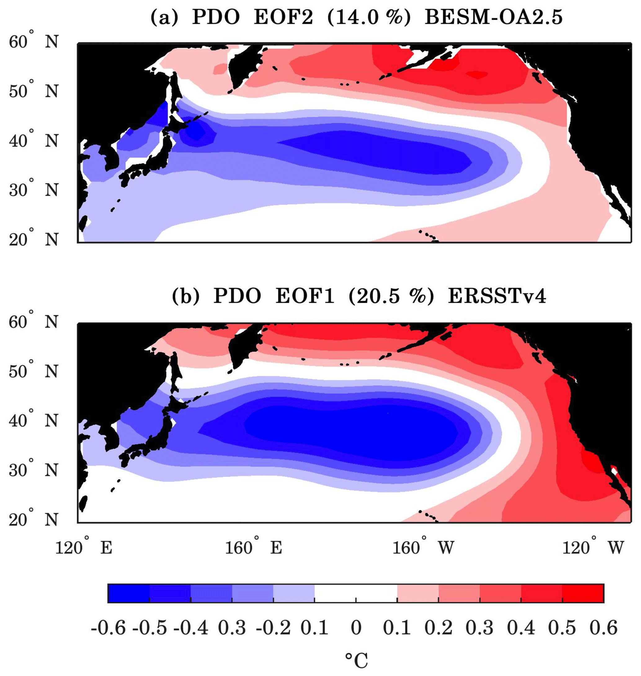
Figure 25 (a) The second EOF modes of monthly SST anomalies of BESM-OA2.5 and (b) the leading EOF mode of monthly SST anomalies of ERSSTv4, both over the North Pacific Ocean (20–60^∘ N, 240–110^∘ W). The results are shown as the monthly SST anomalies regressed onto the corresponding normalized PC time series (degrees Celsius per standard deviation) over the period 1900–2005. The percentages of the variance explained by each EOF are indicated in the titles of the panels. The contour interval is 0.1 ^∘C.

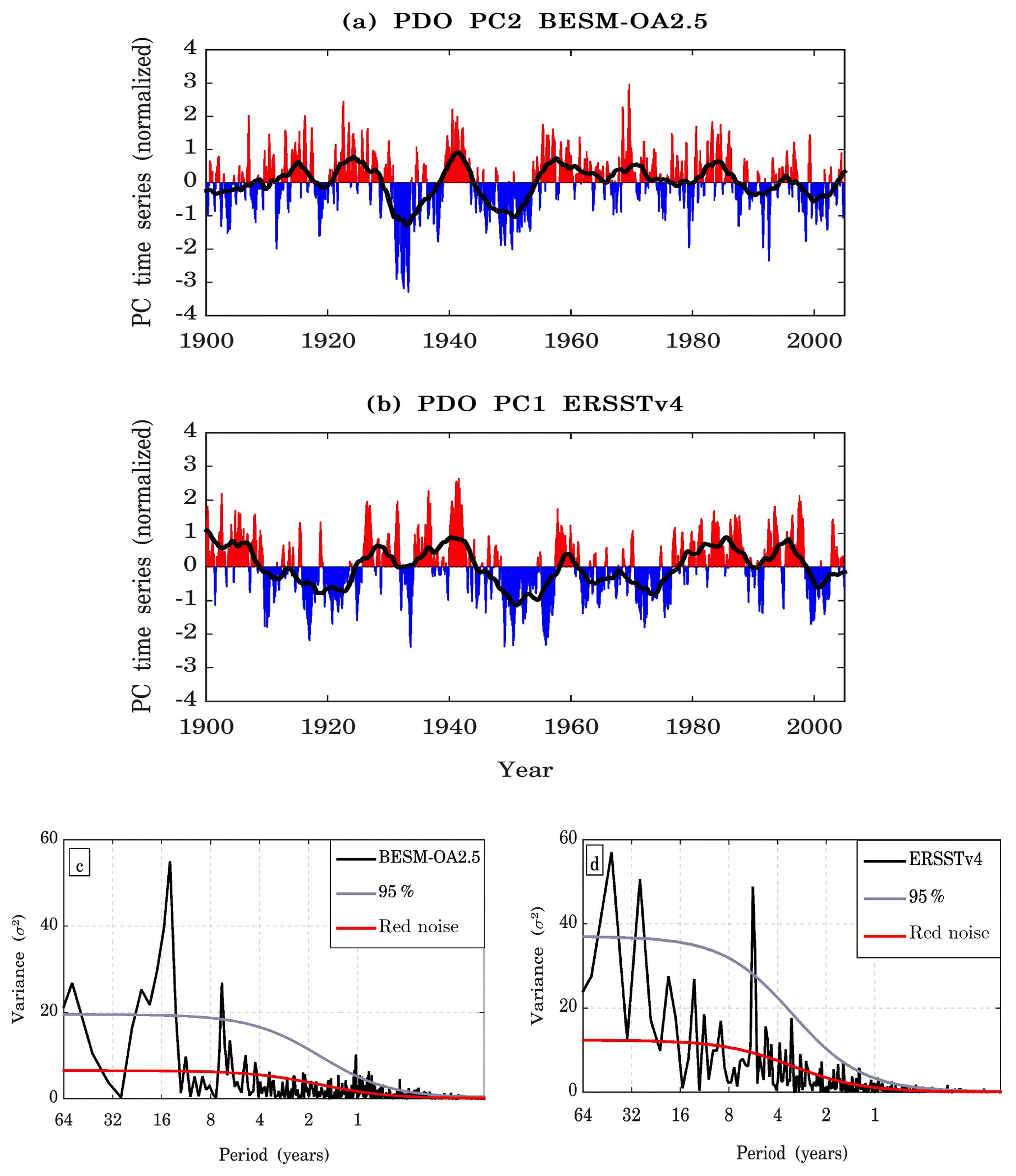
Figure 26 Normalized second PC time series for (a) BESM-OA2.5 and normalized leading PC time series for (b) ERSSTv4 over the period 1900–2005. The solid black lines show the 5-year running average. Panels (c) and (d) show the power spectra of the second PC time series for BESM-OA2.5 and for the leading PC time series for ERSSTv4, respectively. The solid red line represents the theoretical red noise spectrum and the gray line represents the 95 % confidence level.

5 Summary

The ability of Earth system models to project future climate parameters based on conditions given by future scenarios of atmospheric greenhouse gas concentrations can be assessed by how accurately the models can reproduce observed climate features. Therefore, evaluation of how these models perform over historical periods for which there are observations that can be compared with model calculations represents a key part of Earth system modeling. In this study, the BESM-OA2.5 historical simulation was evaluated for the period 1850–2005 following the CMIP5 protocol (Taylor et al., 2012) with a focus on simulations of the mean climate and key large-scale modes of climate variability.

BESM-OA2.5 is an updated version of BESM-OA2.3 (Nobre et al., 2013; Giarolla et al., 2015), which now incorporates the new Brazilian Global Atmospheric Model (BAM; Figueroa et al., 2016). This new version reduced a mean global bias of the energy balance at the top of the atmosphere from −20 to −4 W m⁻². Moreover, systematic errors were reduced in wind, humidity, and temperature in the surface layer over oceanic regions via the inclusion of formulations presented by Jiménez et al. (2012).

The analysis of the mean climate showed that the model can simulate the general mean climate state. Nevertheless, some significant biases appeared in the simulation, such as a double ITCZ over the Pacific and Atlantic oceans and some notable regional biases in the precipitation field (e.g., over the Amazon and Indian regions) and in the SST field (e.g., south of Greenland). Nevertheless, the model has shown an improvement in simulating the ITCZ and a reduction in the global precipitation RMSE compared with that of BESM-OA2.3. BESM-OA2.5 shows a nearly globally positive SST bias that was absent in version 2.3; however, the SST RMSE was slightly reduced in the newer version of the model.

The most relevant climate patterns on interannual to decadal timescales simulated by BESM-OA2.5 were compared with the ones obtained from observations and reanalysis. Over the Pacific, the ENSO was simulated with a lower amplitude of variability than that recorded from the observations, and this weak ENSO seems to impact other Pacific variability patterns, such as the PDO. Conversely, the major phenomena over the Atlantic basin were well represented in BESM-OA2.5 simulations. This was the case for the tropical Atlantic mode of interhemispheric variability (AMM), which was very well simulated by the model in terms of the spatial pattern and temporal variability. It is worth noting that this mode is considered to be poorly simulated by the models used in the Intergovernmental Panel on Climate Change (IPCC) Fifth Assessment Report (AR5; Flato et al., 2013). It is also relevant to highlight the ability of BESM-OA2.5 to represent the enhanced rainfall over the cooler waters of the SW tropical Atlantic that are associated with the South Atlantic Convergence Zone (SACZ). The ability of the model to simulate the AMM and SACZ is an important result, since one of our main aims is to represent the modes that directly impact the precipitation over South America. The AMOC reproduced by BESM-OA2.5 has a meridional overturning structure comparable with the ensemble AMOC simulated by the CMIP5's models. BESM's maximum AMOC strength average value was slighter lower than the average value observed by the RAPID project, but well within the range of the observed root-mean-square variability. Although the averaged maximum strength AMOC simulated by the CMIP5 models is within the observed root-mean-square variability range, most models tend to simulate a strong AMOC, with a maximum strength above 20 Sv, which is outside of the range (Zhang and Wang, 2013). The NAO atmospheric variability, which is well simulated by the CMIP5 models (Ning and Bradley, 2016), is also very well simulated by BESM-OA2.5. In the extratropics, BESM-OA2.5 could reproduce major variabilities in both hemispheres, such as the PNA, PSA, and the SAM teleconnection patterns, relatively well compared to the CMIP5 models, which reproduces the PNA (Ning and Bradley, 2016) and SAM (Zheng et al., 2013).

Similar to Nobre et al. (2013), this study aimed to evaluate BESM-OA2.5 by comparing the most important features of the climate system simulated by the model with observations and reanalysis. The next version of the model (BESM-OA2.9) is already under development. In this new version, the MOM4p1 ocean model has been replaced by the MOM5. Regarding the atmospheric model, new developments have been carried out to improve BAM's capacity, with more sophisticated physics as described by (Figueroa et al., 2016). This new BESM version confronts the challenge of improving the precipitation simulation, in particular alleviating the deficit over the Amazon. The ENSO is a large-scale phenomenon that will be scrutinized to understand the reasons for weak variability. The other feature of the model is the weaker warming when the CO₂ equivalent is used as the only forcing compared with the warming predicted by other CMIP5 models that do not consider the direct and indirect effects of atmospheric aerosols. If BESM-OA2.5 performs consistently with CMIP5 models, then it would underestimate the warming observed over the last decades. Because models can respond in different ways to external forcing, an aim in the near future is to carry out a numerical experiment in which the model is forced with observed aerosol concentration estimates (as a read-in field) to address to what extent BESM is affected. In the future, a study comparing BESM-OA versions 2.5 and 2.9 is planned to fully explore and report the advances made in the modeling work over the last couple of years. Such a study will provide a broader perspective on the technical challenges overcame throughout this project and will assess the improvements achieved in each version of the model for better simulating the climate system.