the Creative Commons Attribution 4.0 License.
the Creative Commons Attribution 4.0 License.
 | 16 Apr 2019
Ocean carbon and nitrogen isotopes in CSIRO Mk3L-COAL version 1.0: a tool for palaeoceanographic research
Pearse J. Buchanan
Richard J. Matear
Zanna Chase
Steven J. Phipps
Nathan L. Bindoff
The isotopes of carbon (δ13C) and nitrogen (δ15N) are commonly used proxies for understanding the ocean. When used in tandem, they provide powerful insight into physical and biogeochemical processes. Here, we detail the implementation of δ13C and δ15N in the ocean component of an Earth system model. We evaluate our simulated δ13C and δ15N against contemporary measurements, place the model's performance alongside other isotope-enabled models and document the response of δ13C and δ15N to changes in ecosystem functioning. The model combines the Commonwealth Scientific and Industrial Research Organisation Mark 3L (CSIRO Mk3L) climate system model with the Carbon of the Ocean, Atmosphere and Land (COAL) biogeochemical model. The oceanic component of CSIRO Mk3L-COAL has a resolution of 1.6∘ latitude × 2.8∘ longitude and resolves multimillennial timescales, running at a rate of ∼400 years per day. We show that this coarse-resolution, computationally efficient model adequately reproduces water column and core-top δ13C and δ15N measurements, making it a useful tool for palaeoceanographic research. Changes to ecosystem function involve varying phytoplankton stoichiometry, varying CaCO3 production based on calcite saturation state and varying N2 fixation via iron limitation. We find that large changes in CaCO3 production have little effect on δ13C and δ15N, while changes in N2 fixation and phytoplankton stoichiometry have substantial and complex effects. Interpretations of palaeoceanographic records are therefore open to multiple lines of interpretation where multiple processes imprint on the isotopic signature, such as in the tropics, where denitrification, N2 fixation and nutrient utilisation influence δ15N. Hence, there is significant scope for isotope-enabled models to provide more robust interpretations of the proxy records.
- Article
(14963 KB) - Full-text XML
-
Supplement
(770 KB) - BibTeX
- EndNote


Elements that are involved in reactions of interest, such as exchanges of carbon and nutrients, experience isotopic fractionation. Typically, the heavier isotope will be enriched in the reactant during kinetic fractionation, in more oxidised compounds during equilibrium fractionation and in the denser form during phase state fractionation (i.e. evaporation). Because fractionation against one isotope relative to the other is minuscule, the isotopic content of a sample is conventionally expressed as a δ value (δhE), where the ratio of the heavy to light element in solution (hE:lE) is compared to a standard ratio (hEstd:lEstd) in units of per mille (‰).
The strength of fractionation against the heavier isotope during a given reaction, ϵ, is also expressed in per mille notation. Fractionation with an ϵ equal to 10 ‰, for example, will involve 990 units of hE for every 1000 units of lE at a hypothetical standard ratio (hEstd:lEstd) of 1:1. At more realistic standard ratios ⋘1:1, say 0.0112372:1 for a δ13C value of 0 ‰, a fractionation at 10 ‰ would involve units of 13C per unit of 12C. Slightly greater preference of one isotope over another in this case involves a preference for the lighter carbon isotope (12C) over the heavier (13C), which enriches the remaining dissolved inorganic carbon (DIC) in 13C and depletes the product. Certain isotopic preferences, or strengths of fractionation, therefore allow certain reactions to be detected in the environment.
The measurement of the stable isotopes of carbon (δ13C) and nitrogen (δ15N) have been fundamental for understanding how these important elements cycle within the ocean (e.g. Schmittner and Somes, 2016; Menviel et al., 2017a; Rafter et al., 2017; Muglia et al., 2018). We will now briefly introduce each isotope in turn.
The distribution of δ13C is dependent on air–sea gas exchange, ocean circulation and organic matter cycling. These contributions make the δ13C signature difficult to interpret, and several modelling studies have attempted to elucidate their roles (Tagliabue and Bopp, 2008; Schmittner et al., 2013). These studies have shown that preferential uptake of 12C over 13C by biology in surface waters enforces strong horizontal and vertical gradients in δ13C of DIC (δ13CDIC), greatly enriching surface waters, particularly in subtropical gyres where vertical exchange with deeper waters is restricted (Tagliabue and Bopp, 2008; Schmittner et al., 2013). Meanwhile, air–sea gas exchange and carbon speciation control the δ13CDIC reservoir over longer timescales (Schmittner et al., 2013). Because air–sea and speciation fractionation are temperature dependent, such that cooler conditions tend to elevate the δ13CDIC of surface waters, they also tend to smooth the gradients produced by biology by working antagonistically to them. Despite this smoothing, biological fractionation drives strong gradients at the surface, which imparts unique δ13C signatures to the water masses that are carried into the interior. These insights have provided clear evidence of reduced ventilation rates in the deep ocean during glacial climates (Tagliabue et al., 2009; Menviel et al., 2017a; Muglia et al., 2018).
δ15N is determined by biological processes that add or remove fixed forms of nitrogen. It therefore records the relative rates of sources and sinks within the marine nitrogen cycle (Brandes and Devol, 2002). Dinitrogen (N2) fixation is the largest source of fixed nitrogen to the ocean, the bulk of which occurs in warm, sunlit surface waters and introduces nitrogen with a δ15N of approximately −1 ‰ (Sigman et al., 2009). Denitrification is the largest sink of fixed nitrogen and occurs in deoxygenated water columns and sediments. Denitrification fractionates strongly against 15N at ∼25 ‰ (Cline and Kaplan, 1975). Fractionation during denitrification is most strongly expressed in the water column where ample nitrate (NO3) is available, making water column denitrification responsible for elevating global mean δ15N above the −1 ‰ of N2 fixers (Brandes and Devol, 2002). Meanwhile, denitrification occurring in the sediments only weakly fractionates against 15N (Sigman et al., 2009), providing only a slight enrichment of δ15N above that introduced by N2 fixation. Variations in δ15N can therefore tell us about global changes in the ratio of sedimentary to water column denitrification, with increases in δ15N associated with increases in the proportion of denitrification occurring in the water column (Galbraith et al., 2013), but it can also reflect regional changes in N2 fixation and denitrification (Ganeshram et al., 1995; Ren et al., 2009; Straub et al., 2013).
However, nitrogen isotopes are also subject to the effect of utilisation, which makes the interpretation of δ15N more complicated. Basically, when nitrogen is abundant, the preference for 14N over 15N increases but when nitrogen is limited this preference disappears (Altabet and Francois, 2001). Complete utilisation of nitrogen therefore reduces fractionation to 0 ‰. While this adds complexity, it also imbues δ15N as a proxy of nutrient utilisation by phytoplankton. As nitrogen supply to phytoplankton is controlled by physical delivery from below, changes in δ15N can be interpreted as changes in the physical supply (Studer et al., 2018). Phytoplankton fractionate against 15N at ∼5 ‰ (Wada, 1980) when bioavailable nitrogen is abundant. If nitrogen is utilised to completion, which occurs in much of the low to midlatitude ocean, then no fractionation will occur and the δ15N of organic matter will reflect the δ15N of the nitrogen that was supplied (Sigman et al., 2009). However, in the case where nitrogen is not consumed towards completion, which occurs in zones of strong upwelling/mixing near coastlines, the Equator and high latitudes, the bioavailable nitrogen pool will be enriched in 15N as phytoplankton preferentially consume 14N. As the remaining bioavailable N is continually enriched in 15N, the organic matter that settles into sediments beneath a zone of incomplete nutrient utilisation will bear this enriched δ15N signal. In combination with modelling (Schmittner and Somes, 2016), the δ15N record is able to provide evidence for a more efficient utilisation of bioavailable nitrogen during glacial times (Martinez-Garcia et al., 2014; Kemeny et al., 2018) and a less efficient one during the Holocene (Studer et al., 2018).
Complimentary measurements of δ13C and δ15N provide powerful, multi-focal insights into oceanographic processes. δ13C is largely a reflection of how water masses mix away the strong vertical and horizontal gradients enforced by biology, while δ15N simultaneously reflects changes in the major sources and sinks of the marine nitrogen cycle and how effectively nutrients are consumed at the surface. However, the interpretation of these isotopes is often difficult. They are subject to considerable uncertainty because there are multiple processes that imprint on the measured values. Our goal is to equip version 1.0 of the Commonwealth Scientific and Industrial Research Organisation Mark 3L (CSIRO Mk3L) climate system model with the Carbon of the Ocean, Atmosphere and Land (COAL) Earth system model with oceanic δ13C and δ15N such that this model can be used for interpreting palaeoceanographic records. First, we introduce CSIRO Mk3L-COAL. Second, we detail the equations that govern the implementation of carbon and nitrogen isotopes. Third, we assess our simulated isotopes against contemporary measurements from both the water column and sediments and compare the model performance against other isotope-enabled models. Finally, as a first test of the model, we take the opportunity to document how changes in ecosystem functioning affect δ13C and δ15N.
The CSIRO Mk3L-COAL couples a computationally efficient climate system model (Phipps et al., 2013) with biogeochemical cycles in the ocean, atmosphere and land. The model is therefore based on the CSIRO Mk3L climate system model, where the “L” denotes that it is a low-resolution version of the CSIRO Mk3 model that contributed towards the third phase of Coupled Model Intercomparison Project (Meehl et al., 2007) and the Fourth Assessment Report of the Intergovernmental Panel on Climate Change (Solomon et al., 2007). See Smith (2007) for a complete discussion of the CSIRO family of climate models. The land biogeochemical component represents carbon, nitrogen and phosphorus cycles in the Community Atmosphere Biosphere Land Exchange (CABLE) (Mao et al., 2011). The ocean component currently represents carbon, alkalinity, oxygen, nitrogen, phosphorus and iron cycles. The atmospheric component conserves carbon and alters its radiative properties according to changes in its carbon content. For this paper, we focus on the ocean biogeochemical model (OBGCM).
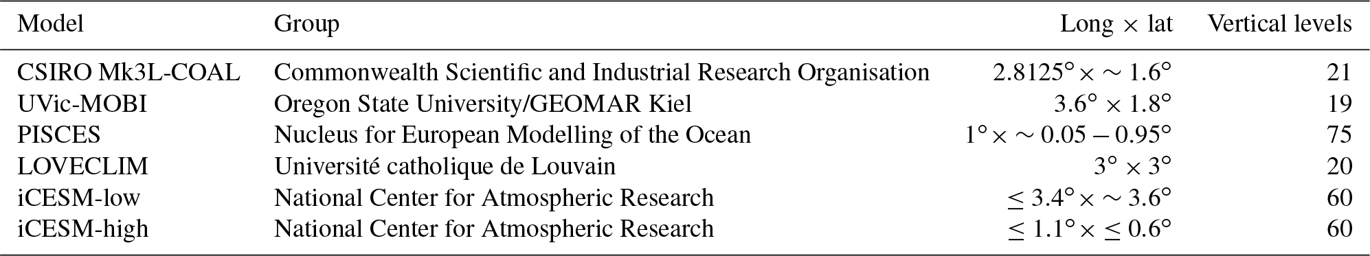
Previous versions of the OBGCM have explored changes in oceanic properties under past (Buchanan et al., 2016), present (Buchanan et al., 2018) and future scenarios (Matear and Lenton, 2014, 2018). These studies demonstrate that the model can reproduce observed features of the global carbon cycle, nutrient cycling and organic matter cycling in the ocean. The OBGCM offers highly efficient simulations of these processes at computational speeds of ∼400 years per day when the ocean general circulation model (OGCM) is run offline (compared to ∼10 years per day in fully coupled mode). The ocean is made up of grid cells of 1.6∘ in latitude by 2.8∘ in longitude, with 21 vertical depth levels spaced by 25 m at the surface and 450 m in the deep ocean (Table 1). The OGCM time step is 1 h, while the OBGCM time step is 1 d. The ability of the OBGCM to reproduce large-scale dynamical and biogeochemical properties of the ocean coupled with its fast computational speed makes the OBGCM useful as a tool for palaeoceanographic research.
2.1 Ocean biogeochemical model (OBGCM)
The OBGCM is equipped with 13 prognostic tracers (Fig. 1). These can be grouped into carbon chemistry fields, oxygen fields, nutrient fields, age tracers and nitrous oxide (N2O). Carbon chemistry fields include DIC, alkalinity (ALK), DI13C and radiocarbon (14C). Radiocarbon is simulated according to Toggweiler et al. (1989). Oxygen fields include dissolved oxygen (O2) and abiotic dissolved oxygen (), a purely physical tracer from which true oxygen utilisation (TOU) can be calculated (Duteil et al., 2013). Nutrient fields include phosphate (PO4), dissolved bioavailable iron (Fe), nitrate (NO3) and 15NO3. Although we define the phosphorus and nitrogen tracers as their dominant species, being PO4 and NO3, these tracers can also be thought of as total dissolved inorganic phosphorus and nitrogen pools. Remineralisation, for instance, implicitly accounts for the process of nitrification from ammonium (NH4) to NO3 (Paulmier et al., 2009) and therefore implicitly includes NH4 and nitrite (NO2) within the NO3 tracer. Age tracer fields include years since subduction from the surface (Agegbl) and years since entering a suboxic zone where O2 concentrations are less than 10 mmol m−3 (Ageomz). Finally, N2O in µmol m−3 is produced via nitrification and denitrification according to the temperature-dependent equations of Freing et al. (2012). All air–sea gas exchanges (CO2, 13CO2, O2 and N2O) and carbon speciation reactions are computed according to the Ocean Modelling Intercomparison Project phase 6 protocol (Orr et al., 2017).
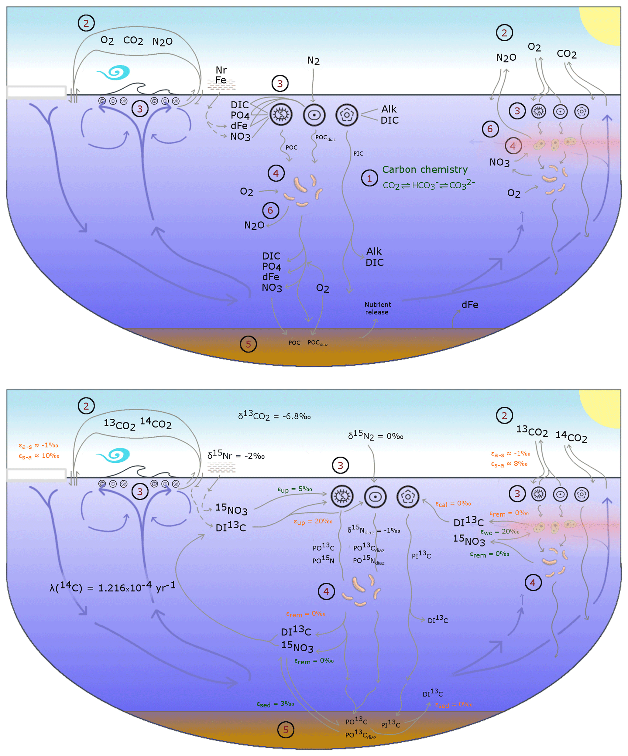
Figure 1A conceptual representation of the ocean biogeochemical model (OBGCM). The bottom panel shows organic matter cycling involving the isotopes of carbon and nitrogen. (1) Carbon chemistry reactions. (2) Air–sea gas exchange. (3) Biological uptake of nutrients and production of organic and inorganic matter. Particulate organic carbon (POC) is produced by the general phytoplankton group and N2 fixers (diazotrophs), while particulate inorganic carbon (PIC) as calcium carbonate (CaCO3) is produced by calcifiers. Export of POC by the general (G) phytoplankton group and N2 fixers (D; diazotrophs) is herein referred to as C and C (see Sect. A1 in the Appendix), respectively. (4) Remineralisation of sinking organic matter under oxic and suboxic conditions. (5) Sedimentary oxic and suboxic remineralisation. (6) Nitrous oxide production and consumption.
Because the isotopes of carbon and nitrogen are influenced by biological processes and there is as yet no accepted standard for ecosystem model parameterisation in the community (see Hülse et al., 2017, for a more detailed discussion), we provide a thorough description of the ecosystem component of the OBGCM in Sect. A in the Appendix. Default parameters for the OBGCM are further provided in Sect. B in the Appendix. Briefly, the ecosystem model simulates the production, remineralisation and stoichiometry (elemental composition) of three types of primary producers: a general phytoplankton group, diazotrophs (N2 fixers) and calcifiers.
3.1 δ13C
The OBGCM explicitly simulates the fractionation of 13C from the total DIC pool, where for simplicity we make the assumption that the total DIC pool represents the light isotope of carbon and is therefore DI12C. Fractionation occurs during air–sea gas exchange, equilibrium reactions and biological consumption in the euphotic zone.
The air–sea gas exchange of 13CO2 is calculated as the exchange of CO2 with additional fractionation factors applied to the sea–air and air–sea components (Zhang et al., 1995; Orr et al., 2017). The flux of 13CO2 across the air–sea interface, F(13CO2), therefore takes the form of CO2 with additional terms that convert to units of 13C in both environments. Without any isotopic fractionation, the equation requires the gas piston velocity of carbon dioxide in m s−1 (), the concentration of aqueous CO2 in both mediums at the air–sea interface in mmol m−3 ( and ) and the ratios of 13C:12C in both mediums (Ratm and Rsea):
A transfer of 13C into the ocean is therefore positive and an outgassing is negative. The Ratm is set to a preindustrial atmospheric δ13C of −6.48 ‰ (Friedli et al., 1986).
The fractionation of carbon isotopes during air–sea exchange involves three components. These are (), a kinetic fractionation that occurs during transfer of gaseous CO2 into or out of the ocean; (), a fractionation that occurs as gaseous CO2 becomes aqueous CO2 (is dissolved in solution); and (), an equilibrium isotopic fractionation as carbon speciates into DIC constituents (H2CO2 ⇔ ⇔ ). The kinetic fractionation during transfer, , is constant at 0.99912, thus reducing the δ13C of carbon entering the ocean by 0.88 ‰. Conversely, carbon outgassing increases the δ13C of the ocean. The fractionations during dissolution () and speciation () are both dependent on temperature. Fractionation during speciation is also dependent on the fraction of relative to total DIC (). These fractionation factors are parameterised as
Dissolution of CO2 into seawater () therefore preferences the lighter isotope and lowers δ13C by between 1.32 ‰ and 1.14 ‰, while the speciation of gaseous CO2 into DIC instead prefers the heavier isotope and raises δ13C by between 10.7 ‰ and 6.8 ‰ for temperatures between −2 and 35 ∘C.
These fractionation factors are applied to the gaseous exchange of CO2 (Eq. 2) to calculate carbon isotopic fractionation.
Because fractionation to aqueous CO2 from DIC () is equal to , a strong preference to hold the heavy isotope in solution exists ( ‰ to −7.9 ‰ between −2 and 35 ∘C). Aqueous carbon that is transferred to the atmosphere is hence depleted in 13C. It is therefore the equilibrium fractionation associated with carbon speciation that is largely responsible for bolstering the oceanic δ13C signature above the atmospheric signature, as it tends to shift 13C towards the oxidised species (), a tendency that strengthens under cooler conditions.
In the default version of CSIRO Mk3L-COAL v1.0, the fractionation of carbon during biological uptake () is set at 21 ‰ for general phytoplankton, 12 ‰ for diazotrophs (e.g. Carpenter et al., 1997) and at 2 ‰ for the formation of calcite (Ortiz et al., 1996). However, a variable fractionation rate for the general phytoplankton group may be activated and depends on the aqueous CO2 concentration (CO2(aq) in mmol m−3) and the growth rate (µ in d−1, as a function of temperature and limiting resources) following Tagliabue and Bopp (2008):
An upper bound of 25 ‰ exists within Eq. (6) when approaches zero but a lower bound does not. We chose to limit to a minimum of 15 ‰ given the reported variations of from culture studies (e.g. Laws et al., 1995).
Biological fractionation of 13C is then applied to the uptake and release of organic carbon.
Because biological fractionation is strong for the general phytoplankton group, which dominates export production throughout most of the ocean, this imparts a negative δ13C signature to the deep ocean. Subsequent remineralisation releases DIC with no fractionation. Finally, the concentration of DI13C is converted into a δ13C via
where 0.0112372 is the Pee Dee Belemnite standard (Craig, 1957).
3.2 δ15N
The OBGCM explicitly simulates the fractionation of 15N from the pool of bioavailable nitrogen. For simplicity, we treat this bioavailable pool as nitrate (NO3), where total NO3 is the sum of 15NO3 and 14NO3. We therefore chose to ignore fractionation during reactions involving ammonium, nitrite and dissolved organic nitrogen, which can vary in their isotopic composition independent of NO3 but represent a small fraction of the bioavailable pool of nitrogen.
The isotopic signatures of N2 fixation and atmospheric deposition, and the fractionation during water column denitrification () and sedimentary denitrification () determine the global δ15N of NO3 (Brandes and Devol, 2002). Biological assimilation () and remineralisation are internal exchanges of the oceanic nitrogen cycle and affect the distribution of δ15NO3. N2 fixation and atmospheric deposition introduce 15NO3 to the ocean with δ15N values of −1 ‰ and −2 ‰, respectively, while biological assimilation, water column denitrification and sedimentary denitrification fractionate against 15NO3 at 5 ‰, 20 ‰ and 3 ‰, respectively (Sigman et al., 2009, Fig. 1).
The accepted standard 15N:14N ratio used to measure variations in nature is the average atmospheric 15N:14N ratio of 0.0036765. To minimise numerical errors caused by the OGCM, we set the atmospheric standard to 1. This scales up the 15NO3 such that a δ15N value of 0 ‰ was equivalent to a 15N:14N ratio of 1:1.
Because we simulate NO3 and 15NO3 as tracers, our calculations require solving for an implicit pool of 14NO3 during each reaction involving 15NO3. The introduction of NO3 at a fixed of −1 ‰ due to remineralisation of N2 fixer biomass provides a simple example with which we can begin to describe our equations. Setting the isotopic value of newly fixed NO3 to −1 ‰ is simple because it removes any complications associated with fractionation. We note, however, that in reality the nitrogenase enzyme does fractionate during its conversion of aqueous N2 (+0.7 ‰) to ammonium and the biomass that is subsequently produced can vary substantially depending of the type of nitrogenase enzyme used (vanadium versus molybdenum based) (McRose et al., 2019). However, we choose to implicitly account for these transformations and considerably simplify them by setting the δ15N of N2 fixer biomass equal to −1 ‰, which reflects the biomass of N2 fixers associated with the more common Mo-nitrogenase.
A of −1 ‰ is equivalent to a 15N:14N ratio of 0.999 in our approach, where 0 ‰ equals a 1:1 ratio of 15N:14N. If the amount of NO3 being added is known alongside its 15N:14N ratio, in this case 0.999 for N2 fixation, we are able to calculate how much 15NO3 is added. We begin with two equations that describe the system.
Ultimately, we need to solve for the change in 15NO3 associated with an introduction of NO3 by N2 fixation. Our known variables are the change in NO3, the δ15N of that NO3 and the 15Nstd∕14Nstd. Our two unknowns are 15NO3 and 14NO3. We must solve for 14NO3 implicitly by describing it according to 15NO3 by rearranging Eq. (11).
This allows us to replace the 14NO3 term in Eq. (10), such that
In our example of N2 fixation, we know the δ15N of the newly added NO3 as being −1 ‰. We also know 15Nstd∕14Nstd as equal to 1:1, or 1. Our equation is simplified.
We can now solve for 15NO3 by rearranging the equation.
The same calculation is applied to NO3 addition via atmospheric deposition, except at a constant fraction of 0.998 (δ15N ‰), and can be applied to any addition or subtraction of 15NO3 relative to NO3 where the isotopic signature is known.
Fractionating against 15NO3 during biological assimilation (), water column denitrification () and sedimentary denitrification () involves more considerations because we must account for the preference of 14NO3 over 15NO3. We begin with an ϵ of 5 ‰ for biological assimilation. This is equivalent to a 15NO3:14NO3 ratio of 0.995 when our atmospheric standard is equal to 1:1 using the following equation.
Note that a positive ϵ value returns a 15NO3:14NO3 ratio <1, while a negative δ15N in the previous example with N2 fixation also returned a 15NO3:14NO3 ratio <1. This works because the reactions are in opposite directions. N2 fixation adds NO3, while assimilation removes NO3. This means that 0.995 units of 15NO3 are assimilated per unit of 14NO3. As we have seen, a more useful way to quantify this is per unit of NO3 assimilated into organic matter. Using Eq. (15), we find that ∼0.4987 units of 15NO3 and ∼0.5013 units of 14NO3 are assimilated per unit (1.0) of NO3 when ϵ equals 5 ‰. Biological assimilation therefore leaves slightly more 15N in the unused NO3 pool relative to 14N, which increases the δ15N of NO3 while creating more 15N-deplete organic matter (δ15Norg).
However, we must also account for the effect that NO3 availability has on fractionation. The preference of 14NO3 over 15NO3 strongly depends on the availability of NO3, such that when NO3 is abundant the preference for the lighter isotope will be strongest. This preference (fractionation) becomes weaker as NO3 is depleted because cells will absorb any NO3 that is available irrespective of its isotopic composition (Mariotti et al., 1981). Thus, as NO3 is utilised, u, towards 100 % of its availability (u=1), the fractionation against 15NO3 decreases to an ϵ of 0 ‰. This means that when u is equal to 1, no fractionation occurs and equal parts 15N and 14N (0.5:0.5 per unit NO3) are assimilated. As we are interested in long timescales, we chose the accumulated product equations (Altabet and Francois, 2001) to approximate this process, where
For numerical reasons, we limited the domain of u to (0.001,0.999) rather than (0,1), such that the utilisation-affected ϵu has a range of −4.997 to −0.035 ‰ for an ϵ of 5 ‰. ϵu is then converted into ratio units by dividing by 1000 and added to the ambient 15N:14N of NO3 in the reactant pool to determine the 15N:14N of the product. In this case, it is the 15N:14N of newly created organic matter but could also be unused NO3 effluxed from denitrifying cells in the case for denitrification.
We then solve for how much 15NO3 is assimilated into organic matter using Eq. (15) because we now know the change in NO3 (ΔNO3) and the 15N:14N of the product, which is 15Norg∕14Norg in our example of biological assimilation.
Here, the change in 15NO3 is equivalent to that assimilated into organic matter. Following assimilation into organic matter, the release of 15NO3 through the water column during remineralisation occurs with no fractionation, such that the same δ15N signature is released throughout the water column.
We apply these calculations to each reaction in the nitrogen cycle that involves fractionation (assimilation, water column denitrification and sedimentary denitrification). They could be applied to any form of fractionation process with knowledge of ϵ, the isotopic ratio of the reactant, the amount of reactant that is used and the total amount of reactant available.
CSIRO Mk3L-COAL adequately reproduces the large-scale thermohaline properties and circulation of the ocean under preindustrial conditions in numerous prior studies (Phipps et al., 2013; Matear and Lenton, 2014; Buchanan et al., 2016, 2018). Rather than reproduce these studies, we concentrate here on how the biogeochemical model performs relative to measurements of δ13C and δ15N in the water column (Eide et al., 2017, data courtesy of the Sigman Lab at Princeton University) and in the sediments (Tesdal et al., 2013; Schmittner et al., 2017). We make these model–data comparisons alongside other isotope-enabled ocean general circulation models (Table 1).
All analyses of model performance were undertaken using the default parameterisation of the biogeochemical model, which is summarised in the tables of Sect. B in the Appendix. Each experiment was run towards steady state under preindustrial atmospheric conditions over many thousands of years. All results presented in this paper therefore reflect tracers that have achieved an equilibrium solution. We present annual averages of the equilibrium state in the following analysis.
Table 1Models assessed against isotope data. The University of Victoria – Model of Ocean Biogeochemistry and Isotopes (UVic-MOBI) fields taken from Schmittner and Somes (2016). Pelagic Interactions Scheme for Carbon and Ecosystem Studies (PISCES) fields provided by Laurent Bopp. LOch–Vecode-Ecbilt-CLio-agIsm Model (LOVECLIM) fields taken from Menviel et al. (2017a). The isotope-enabled Community Earth System Model (iCESM) fields for δ13C (low resolution) provided by Alexandra Jahn (Jahn et al., 2015) and those for δ15N (high resolution) provided by Simon Yang (Yang and Gruber, 2016). PISCES and CESM model resolutions have a range of longitude–latitude spacings to reflect regions of finer resolution, including the Equator and polar regions.
4.1 δ13C of dissolved inorganic carbon (δ13CDIC)
The recent reconstruction of preindustrial δ13CDIC by Eide et al. (2017) provides a large dataset for comparison. We chose this dataset over the compilation of point location water column data of Schmittner et al. (2017) because it offers a gridded product where short-term and small-scale variability are smoothed, making for more appropriate comparison with model output.
Predicted values of δ13CDIC from CSIRO Mk3L-COAL broadly replicated the preindustrial distribution. The predicted global mean of 0.41 ‰ reflected that of the reconstructed mean of 0.42 ‰ (Table 2). Spatial agreement was acceptable with a global correlation of 0.80 (G marker in Fig. 2). Regionally, the Southern Ocean performed well with the lowest root mean square (rms) error of 0.42 ‰, while a greater degree of disagreement in the values of δ13CDIC existed in the middle and lower latitudes of each major basin, particularly in the Atlantic where model–data agreement (correlation, rms error and normalised standard deviation) was poorest. Subsurface δ13CDIC was too low in the tropics of the major basins by ∼0.2 ‰ and too high in the North Pacific and North Atlantic by 0.4 ‰ to 0.6 ‰ (Fig. 3).
Eide et al. (2017)Table 2Comparison of global and region mean δ13CDIC between observations (Eide et al., 2017) and model simulations. Means are annual averages and do not include the Arctic or the upper 200 m of the water column. All data were regridded onto the CSIRO Mk3L-COAL grid space.

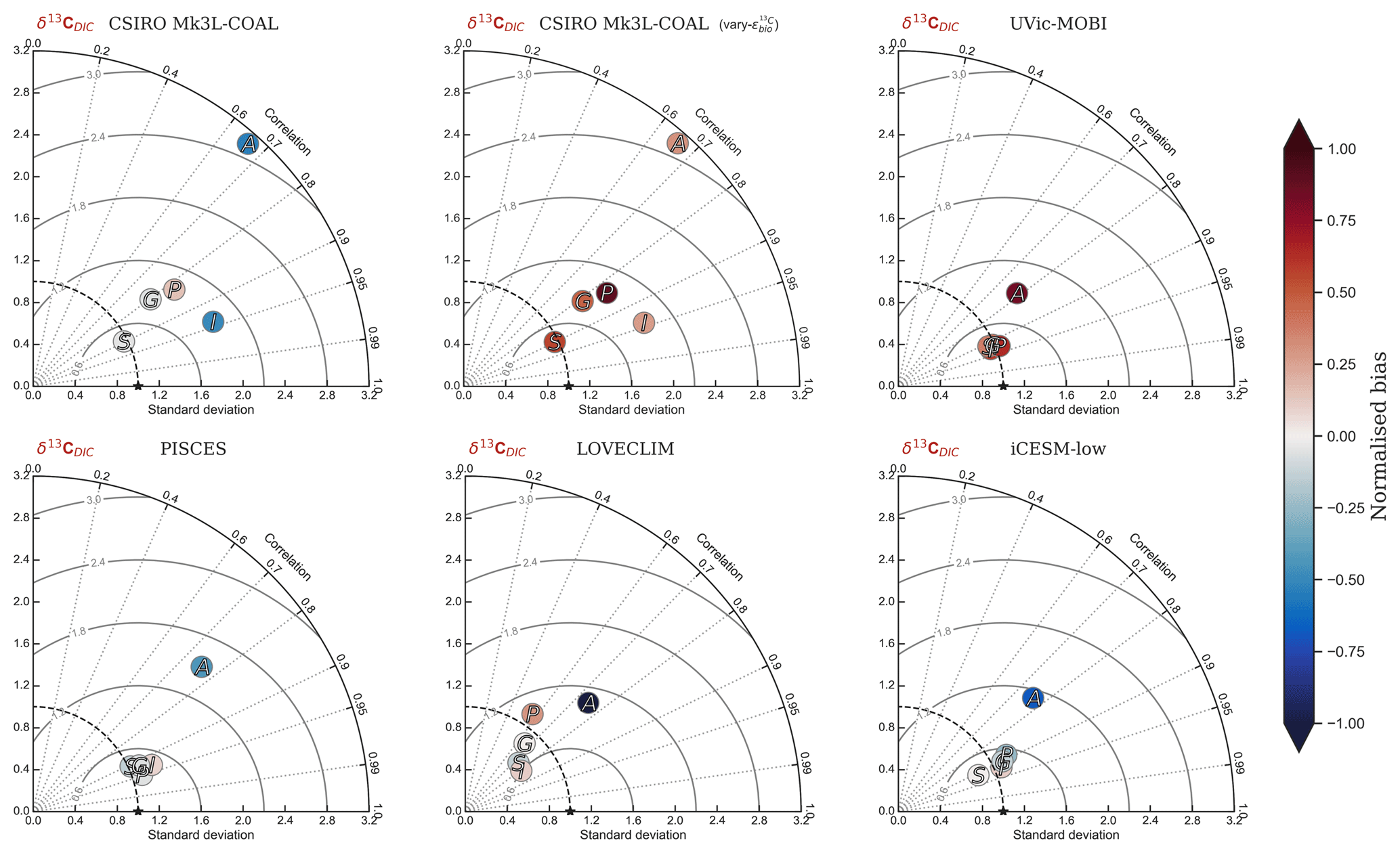
Figure 2Global and regional fits between data (Eide et al., 2017) and simulated δ13C of dissolved inorganic carbon displayed as Taylor diagrams (Taylor, 2001). Shading of the markers represents normalised bias. G indicates global; S indicates Southern Ocean (90–40∘ S); A indicates Atlantic (40∘ S–70∘ N); P indicates Pacific (40∘ S–70∘ N); I indicates Indian Ocean (40∘ S–70∘ N). Measures of fit do not include the Arctic or the upper 200 m of the water column. All data were regridded onto the CSIRO Mk3L-COAL grid space before comparison.
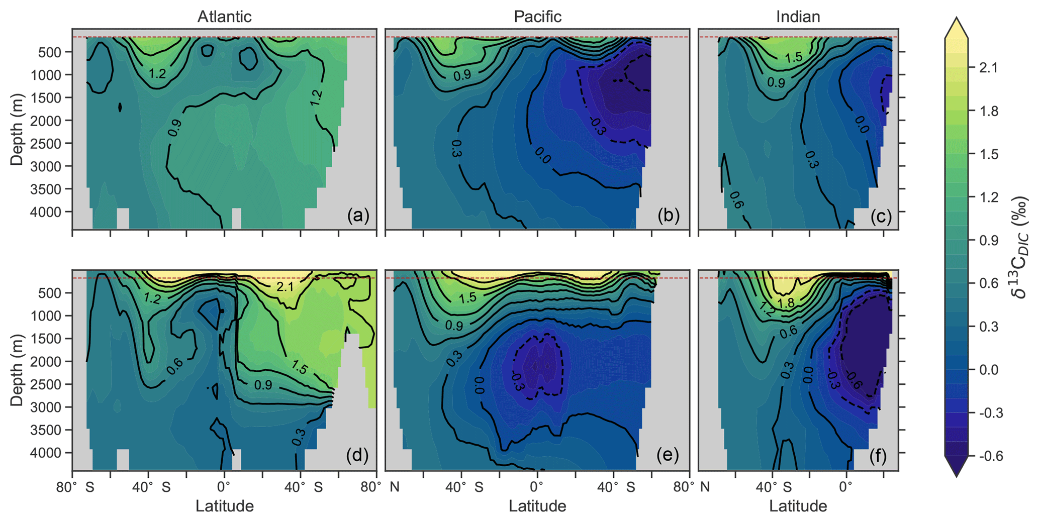
Figure 3Zonal mean observed (a, b, c) and modelled (d, e, f) δ13C of DIC produced by CSIRO Mk3L-COAL for each major basin. The red dashed line marks the upper 175 m and is used for comparison between observed and modelled distributions. Replicate figures for the other models are available in the Supplement.
These inconsistencies were likely related to physical and biological limitations of CSIRO Mk3L-COAL. δ13CDIC in subsurface tropical waters was too low because restricted horizontal mixing and high carbon export drove very negative δ13CDIC values. The very negative δ13C values were associated with very large oxygen minimum zones and were thus a product of poorly represented, fine-scale equatorial dynamics. Coarse-resolution OGCMs are known to have weak equatorial undercurrents that lead to oxygen minimum zones that are too large (Matear and Holloway, 1995; Oschlies, 2000) and CSIRO Mk3L-COAL is no exception. Alternatively, the large oxygen minimum zones could be due to our conservative treatment of organic matter remineralisation (Sect. A in the Appendix), where remineralisation is prevented when O2 and NO3 are unavailable. Organic matter therefore falls deeper into the interior through oxygen-deficient zones, leading to their vertical expansion. Almost certainly, however, it was the poorly represented dynamics within the Pacific basin that were responsible for high δ13CDIC in the subsurface North Pacific, which contains low O2 and low δ13CDIC water due to northward transport from the tropics.
Another inconsistency was a positive bias in the upper 200–500 m, with values exceeding 2 ‰ in many areas of the lower latitudes. However, values as high as 2 ‰ have been measured in the upper 500 m of the Indo-Pacific (Schmittner et al., 2017). Given the difficulties associated with accounting for the Suess effect (invasion of isotopically light fossil fuel CO2), it is possible that the upper ocean values of Eide et al. (2017) underestimate the preindustrial δ13CDIC surface field. It is also equally possible that a fixed biological fractionation () of 21 ‰ may have driven unrealistic enrichment in the simulated field. High growth rates are thought to lower the strength of fractionation during carbon fixation (Laws et al., 1995). To explore the possibility of model–data mismatch caused by our choice to fix at 21 ‰, we implemented biological fractionation that is dependent on phytoplankton growth rate and aqueous CO2 concentration (Eq. 6). We found the implementation of a variable reduced high values in the upper part of the low-latitude ocean but that this reduction was small (Fig. 4). The overwhelming effect was an increase in δ13CDIC throughout the interior, itself caused by weaker fractionation in the tropical ocean. Global mean δ13CDIC subsequently increased by 0.25 ‰. Meanwhile, model skill was unaffected (see CSIRO Mk3L-COAL (vary-) in Fig. 2). Neither fixed nor variable biological fractionation could reproduce the low upper ocean values of the data.
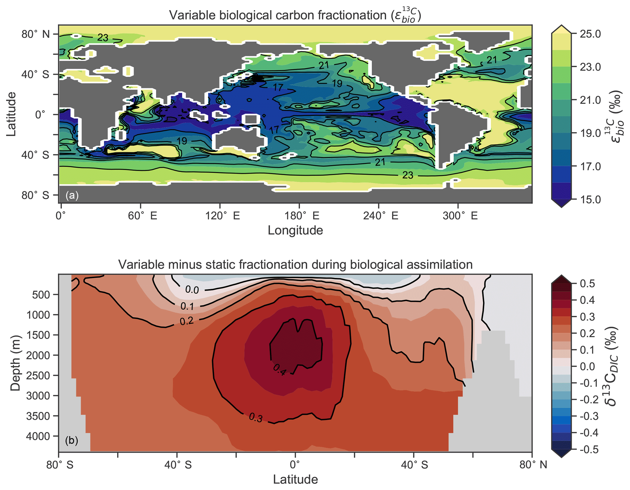
Figure 4The introduction of variable carbon fractionation by phytoplankton (a) and the consequent change in δ13CDIC represented as a zonal mean (b) relative to a case where is fixed at 21 ‰.
It is helpful to place our predicted δ13CDIC alongside those of other global ocean models (Fig. 2; Table 2), both for skill assessment and to further understand the cause of the positive bias in the upper ocean. We take annually averaged, preindustrial δ13CDIC distributions from the UVic-MOBI, PISCES, LOVECLIM and iCESM-low biogeochemical models, most of which have been used in significant palaeoceanographic modelling studies (Menviel et al., 2017a; Tagliabue et al., 2009; Schmittner and Somes, 2016). Predicted δ13CDIC performs adequately in CSIRO Mk3L-COAL relative to these state-of-the-art models. LOVECLIM showed good fit in terms of global and regional means (Table 2) but had lower correlations (Fig. 2), suggesting that its values were accurate but its distribution biased. UVic-MOBI had high correlations, but it consistently overestimated the preindustrial field by ∼0.2 ‰. Interestingly, the bias of UVic-MOBI, which treats biological fractionation as a function of growth rate and aqueous CO2, is similar to CSIRO Mk3L-COAL when this form of fractionation was activated (vary-). PISCES and iCESM-low were the best performing models, equally demonstrating high correlations, low biases, accurate regional and global means and the lowest rms errors. This is perhaps not surprising considering the significantly finer vertical resolutions of these OGCMs and their more complex horizontal grid structure that enables an improved representation of ocean dynamics (Table 1). However, all models performed most poorly in the Atlantic Ocean, with poor correlations, high variability and greater biases.
Returning to the consistent positive bias in the upper ocean, most models (except iCESM-low) predicted upper ocean δ13CDIC ≥ 2.0 ‰ (Figs. S1, S2, S3 and S4 in the Supplement) similar to CSIRO Mk3L-COAL. As each model has a unique representation of the marine ecosystem and consequently a unique treatment of biological fractionation, the common prediction of high upper ocean δ13C once more suggests that the upper ocean values between 200 and 500 m of Eide et al. (2017) may be too low. The underestimation of δ13CDIC may be due to a neglect of biology introducing anthropogenic, isotopically depleted carbon to surface and subsurface layers via remineralisation (the biological Suess effect). This would in turn suggest that a higher global mean of 0.73 ‰ generated from a global compilation of foraminiferal δ13C (Schmittner et al., 2017) is perhaps a more accurate representation of preindustrial δ13C values.
Overall, CSIRO Mk3L-COAL performed acceptably in terms of its mean values and correlations but had consistently greater rms errors in major basins outside of the Southern Ocean. This indicates that CSIRO Mk3L-COAL exaggerated regional minima and maxima as discussed. Despite the regional biases of CSIRO Mk3L-COAL, the comparison demonstrates that all models have strengths and weaknesses. Given its low resolution and computational efficiency, CSIRO Mk3L-COAL performs adequately among other biogeochemical models in its simulation of δ13CDIC.
4.2 δ13C of Cibicides foraminifera (δ13CCib)
We extended our assessment of modelled δ13CDIC by comparing it to a compilation of benthic δ13C measured within the calcite of foraminifera from the genus Cibicides (Schmittner et al., 2017), a genus on which much of the palaeoceanographic δ13C records are based. For this comparison, we adjusted our predicted δ13CDIC to predicted δ13CCib using the linear dependence on carbonate ion concentration and depth suggested by Schmittner et al. (2017):
This adjustment accounts for slight fractionation during incorporation of DIC into foraminiferal calcite and is found to be partly explained by the concentration of ions and pressure. A one-to-one comparison between δ13CDIC and δ13CCib hence introduces some degree of error since this fractionation is not accounted for. Because we are interested in applying simulated δ13CDIC to a palaeoceanographic context, we must first be able to convert our simulated δ13CDIC to δ13CCib in an effort to make better comparisons, particularly as the distribution of is subject to change. By adjusting our three-dimensional δ13CDIC output using Eq. (21), we attain predicted δ13CCib (see inset titled “calibration” in Fig. 5). For good measure, we also computed measures of statistical fit for a traditional one-to-one comparison between δ13CDIC and δ13CCib to assess the benefit of the calibration.
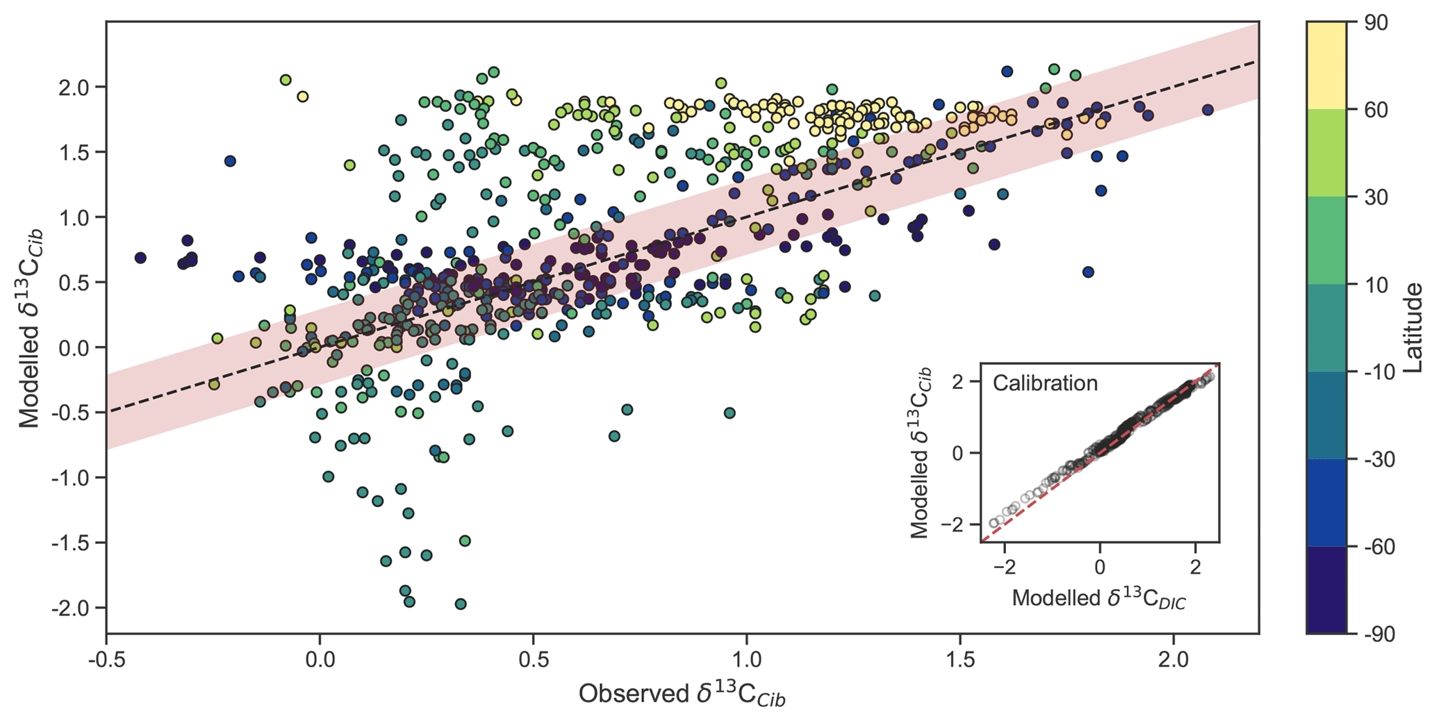
Figure 5Measured versus modelled δ13CCib (N=690) of CSIRO Mk3L-COAL coloured by latitude. Red shading about the 1:1 line is an estimate of the variability implicit in the relationship between δ13CCib and δ13CDIC of Schmittner et al. (2017). The inset on the bottom right shows the effect of the calibration of Eq. (21).
Measured δ13CCib data from Schmittner et al. (2017) were binned into model grid boxes and averaged for the comparison. Those measurements that fell within the OGCM's land mask were excluded. Transfer and averaging onto the coarse-resolution OGCM grid reduced the number of points for comparison from 1763 to 690, lowered the mean of measured δ13CCib from 0.76 ‰ to 0.52 ‰ and reduced the absolute range from to .
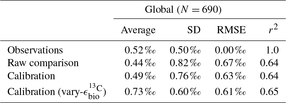
Adjusted δ13CCib using Eq. (21) showed good fit to measured δ13CCib given the sparsity of data, with a global correlation of 0.64, a mean of 0.57 ‰ and an rms error of 0.63 ‰ (Table 3). If a one-to-one relationship between δ13CDIC and δ13CCib was used, the global correlation was not affected and only slightly worse skill was detected in mean, rms error and standard deviation. Accounting for the regional influence of carbonate ion concentration and depth was therefore beneficial, likely because very negative and positive values were slightly adjusted towards the mid-range (inset in Fig. 5), but this was not necessary for an adequate comparison. This conclusion was also reached by Schmittner et al. (2017). Likewise, implementing variable fractionation by phytoplankton () had little effect except to increase values and slightly improve measures of skill (Table 3). Of the 690 data points used in the comparison, 419 fell within the error around what could be considered a good fit (shaded red area in Fig. 5). The error was taken as 0.29 ‰ and represents the standard deviation associated with the relationship between δ13CDIC and δ13CCib measurements (Schmittner et al., 2017).
Table 3Statistical comparison of core-top δ13CCib with predicted values produced by the CSIRO Mk3L-COAL ocean model.
Some notable over and underestimation occurred in the adjusted δ13CCib output that more or less mirrored those inconsistencies previously discussed for δ13CDIC. Values as low as −1.9 ‰, well below measured δ13CCib minima of −0.7 ‰, existed in the equatorial subsurface Pacific and Indian oceans (i.e. where the oxygen minimum zones existed). This can be seen in Fig. 5, where some values in the equatorial band are well below the shaded region of good fit. Meanwhile, very high values of δ13CCib were predicted in Arctic surface waters. The exaggeration of these local minima and maxima reflects those found in the modelled δ13CDIC distribution. Despite these local inconsistencies, CSIRO Mk3L-COAL shows good potential for direct comparisons to palaeoceanographic data sets of foraminiferal δ13C with or without calibration.
4.3 δ15N of nitrate ()
We produced univariate measures of fit by comparing measurements of with equivalent values from CSIRO Mk3L-COAL at the nearest point (Fig. 6; Table 4). Measured values were collected over a 30-year period using a variety of collection and measurement methods with a distinct bias towards the Atlantic Ocean. To try and remove some temporal and spatial bias, we binned and averaged measurements into equivalent model grids.
Table 4Comparison of global and region mean between observations and model simulations. Model means are annual averages. All data were regridded onto the CSIRO Mk3L-COAL grid space. The δ15N data (5330 measurements courtesy of the Sigman Lab, Princeton University) were binned into corresponding grid boxes and averaged for direct comparison, which reduced the data to 2532 points. More than one data point of δ15N may therefore contribute to each simulated value.
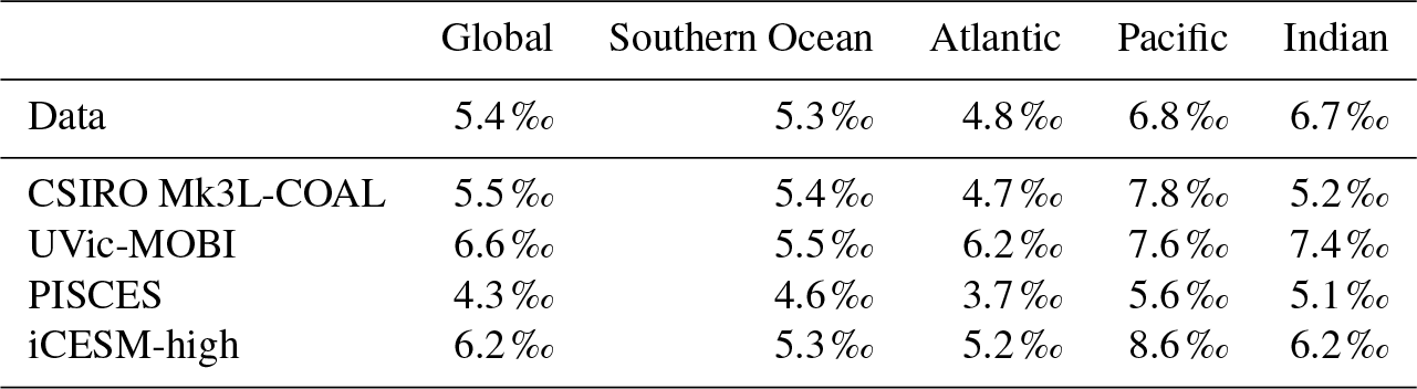

Figure 6Global and regional fits between observations and simulated displayed as Taylor diagrams (Taylor, 2001). Shading of the markers represent normalised bias. G indicates global; S indicates Southern Ocean (90–40∘ S); A indicates Atlantic (40∘ S–70∘ N); P indicates Pacific (40∘ S–70∘ N); I indicates Indian Ocean (40∘ S–70∘ N). The δ15N data (5330 measurements courtesy of the Sigman Lab, Princeton University) were binned into corresponding grid boxes and averaged for direct comparison, which reduced the data to 2532 points. More than one data point of δ15N may therefore contribute to each simulated value.
CSIRO Mk3L-COAL adequately reproduced the global patterns of . We found excellent agreement in the volume-weighted means of (Table 4). Tight agreement in the means was a consequence of reproducing similar values where the majority of observed data existed. Most measurements have been taken from the upper 1000 m in the North Atlantic where values cluster at just under 5 ‰ (see Fig. 7a, c, e). Closer inspection of the Atlantic using depth and zonally averaged sections (Figs. 8 and 9) revealed that the model adequately reproduced the low δ15N signature of ∼4 ‰ caused by N2 fixation occurring in the tropical Atlantic (Marconi et al., 2017). A basin-wide rate of Atlantic N2 fixation equal to ∼33 Tg N yr−1 lowered Atlantic values below 5 ‰ and was fundamental for reproducing the observations. Outside the Atlantic, where data are more sparse, the model successfully reproduced the meridional gradients across the Antarctic, Subantarctic and subtropical zones, the subsurface maxima in the tropics of all major basins and the tongues of high and low values in surface waters of the Pacific consistent with changes in nitrate utilisation (Figs. 8 and 9).
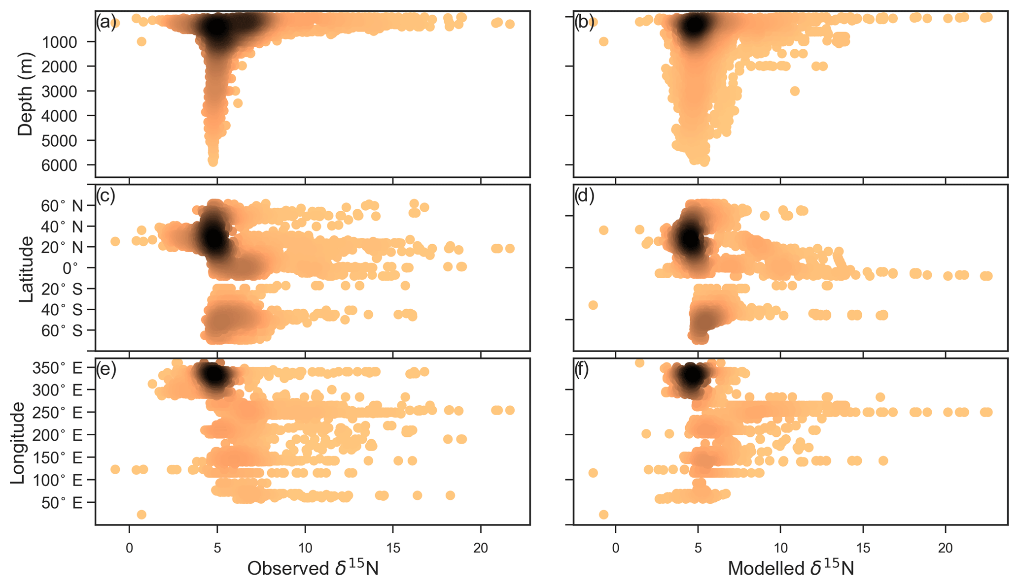
Figure 7Observed (a, c, e) and modelled (b, d, f) δ15N of NO3 data (N=5004) plotted against depth (a, b), latitude (c, d) and longitude (e, f). Colour shading represents the density of data, such that the darker a mass of data points is, the more data are represented there.
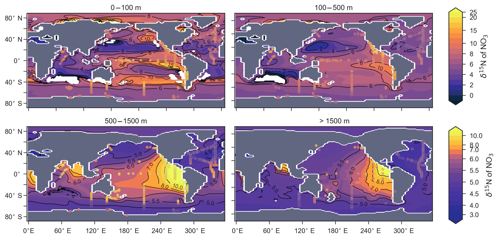
Figure 8Depth-averaged sections of modelled (colour contours) and observed (overlaid markers) .

Figure 9Zonally averaged sections of modelled (colour contours) and observed (overlaid markers) . The global zonal average encompasses all basins.
Some important regional inconsistencies between the simulated and measured values did exist (refer to Figs. 8 and 9) and degraded the correlation. Much like the high values of δ13CDIC that were transported too deeply into the North Atlantic interior, a low signature was transported too far into the deep North Atlantic. CSIRO Mk3L-COAL therefore underestimated deep before mixing through to the South Atlantic restored values towards the measurements. Subsurface values in the North Pacific were also underestimated, which can be attributed to the inability of the coarse-resolution OGCM to transport low O2, high water northwards from the eastern tropical Pacific. Simulated values in the Indian Ocean, specifically near the Arabian Sea, significantly underestimated the data because the suboxic zone was misrepresented in the Bay of Bengal. Misrepresentation of the northern Indian Ocean was responsible for very poor model–data fit in the Indian Ocean (Fig. 6). Meanwhile, the deep (>1500 m) eastern tropical Pacific tended to overestimate the data, due to a large, deep, unimodal suboxic zone. These physically driven inconsistencies in the oxygen field are common to other coarse-resolution models (Oschlies et al., 2008; Schmittner et al., 2008) and, like the δ13C distribution, were the main cause of the misfit between simulated and observed . The correlations reflected these regional under- and overestimations, particularly in the Indian Ocean.
Finally, we placed CSIRO Mk3L-COAL in the context of other isotope-enabled global models: UVic-MOBI, PISCES and iCESM-high (Table 1). This comparison demonstrated that the modelled distribution of was adequately placed among the current generation of models. The global and regional means were more accurately reproduced by CSIRO Mk3L-COAL than for UVic-MOBI, PISCES and iCESM-high (Table 4; also see shading in Fig. 6). Atlantic was best reproduced by CSIRO Mk3L-COAL. Meanwhile, correlations tended to be slightly lower for CSIRO Mk3L-COAL than UVic-MOBI and iCESM-high, and consistently lower than PISCES (Fig. 6). UVic-MOBI underestimated the data but produced high correlations in the Southern Ocean and globally. Regionally, PISCES was best correlated to the measurements of of the three models, although it had a consistent positive bias. iCESM-high was acceptably correlated with the data in the global sense but was highest in rms errors, particularly in the Pacific. CSIRO Mk3L-COAL therefore showed an acceptable measure of fit to the noisy and sparse data and reproduced most regional patterns, albeit with misrepresentation in the Indian Ocean and some exaggerations of local minima/maxima as discussed. Future model–data comparisons with CSIRO Mk3L-COAL should therefore take these limitations into account. Overall, however, we find that CSIRO Mk3L-COAL broadly reproduced the data. Annual rates of N2 fixation, water column denitrification and sedimentary denitrification at roughly 122, 52 and 78 Tg N yr−1, respectively, produced this agreement.
An important caveat to the routines of CSIRO Mk3L-COAL should be noted. CSIRO Mk3L-COAL underwent significant tuning of water column and sedimentary denitrification parameterisations in order to reproduce known values of during development. One important parameter is the lower threshold of NO3 concentration at which point water column denitrification is shut off (Sect. A2.3). In CSIRO Mk3L-COAL, this is set at 30 mmol m−3, which is an arbitrary limit that was implemented to prevent water column denitrification from reducing NO3 to zero in the large suboxic zones. Hence, a caveat of the current model is an inability for water column and sedimentary denitrification to realistically adjust as suboxia changes. However, the parameterisation does allow for targeted experiments where the ratio of water column to sedimentary denitrification can be controlled if, for instance, it is unclear how water column and sedimentary denitrification respond to certain conditions. This is currently the case during the Last Glacial Maximum, where expansive suboxic zones in the Pacific (Hoogakker et al., 2018) were counter-intuitively associated with reduced rates of water column denitrification (Ganeshram et al., 1995). We have, in this version, chosen to keep this parameterisation and note that future developments will focus on dynamic responses to variations in suboxia.
4.4 δ15N of organic matter (δ15Norg)
CSIRO Mk3L-COAL tracks the δ15N signature of organic matter (δ15Norg) that is deposited in the sediments. We compared the simulated δ15Norg to the core-top compilation of Tesdal et al. (2013) with 2176 records of δ15Norg. These records were binned and averaged onto the CSIRO Mk3L-COAL ocean grid, such that the 2176 records became 592. When comparing sediment core-top measurements of δ15N to that of the model, it is necessary to consider how δ15Norg is altered by early burial. As records in the compilation of Tesdal et al. (2013) are from bulk nitrogen, we can assume that the “diagenetic offset” as described by Robinson et al. (2012) is active. The diagenetic offset involves an increase in the δ15N of sedimentary nitrogen of between 0.5 ‰ and 4.1 ‰ relative to that of sinking particulate organic matter and appears to be related to pressure (Robinson et al., 2012), although the reasoning behind this relationship remains to be defined.
In light of the diagenetic offset, we make three comparisons with the compilation of Tesdal et al. (2013). A raw comparison is made, alongside an attempt to account for the diagenetic offset using two depth-dependent corrections (Table 5 and Fig. 10):
The first correction () is taken from Robinson et al. (2012), while the second () originates from how Schmittner and Somes (2016) treated sedimentary nitrogen isotope data in their study of the Last Glacial Maximum. Both are based on the observation that the diagenetic offset increases with pressure, in this case represented by depth (z) in kilometres (km).
Table 5Statistical comparison of core-top δ15Norg with predicted values of the CSIRO Mk3L-COAL ocean model. The corrected vales ( and ) account for alteration during early diagenesis following burial.

Following binning and averaging onto the model grid, the raw comparison immediately showed a consistent underestimation of the core-top data, with a predicted mean of 2.7 ‰ well below the observed mean of 4.7 ‰. Our correlation was 0.27, which indicates a limited ability to replicate regional patterns. This underestimation and low correlation is easily seen when predicted values are compared directly to the core-top data in Fig. 10. Like the nitrogen isotope model of Somes et al. (2010), we find that the offset between simulated and observed core-top bulk δ15Norg is roughly equivalent to the observed average diagenetic offset of ‰. This indicates that diagenetic alteration of δ15Norg is active during early burial in the core-top data.
Including a diagenetic offset therefore improved agreement between our predicted δ15Norg and the core-top data considerably (Table 5 and Fig. 10). Both corrections accounted for the enrichment of δ15N in deeper regions and the minor diagenetic alteration in areas of high sedimentation that typically occurs in shallower sediments. The average δ15Norg increased to 4.5 ‰ for and 5.2 ‰ for . Correlations increased from 0.27 to 0.47 and 0.53, respectively. The improvement was clearly observed in the Southern Ocean, where both the magnitude and spatial pattern of δ15Norg were well replicated by the model. Changes in the Southern Ocean over glacial–interglacial cycles reflect shifts in the global marine nitrogen cycle and nutrient utilisation (Martinez-Garcia et al., 2014; Studer et al., 2018), and the ability of CSIRO Mk3L-COAL to account for these patterns in the core-top data is encouraging for future study. We suggest that future palaeoceanographic model–data comparisons of δ15Norg use the depth correction of Schmittner and Somes (2016) as it provided the best correlations and reproduced Southern Ocean δ15Norg at 0.5 ‰ greater than the global mean (see Table 5).

Figure 10Direct comparison of observed versus modelled δ15Norg incident on the sediments. Panels (a), (c) and (e) show spatial distribution of simulated δ15Norg overlain by core-top data from the compilation of Tesdal et al. (2013). Panels (b), (d) and (f) compare all core-top data against simulated δ15Norg. Panels (a) and (b) depict raw output of the model, while panels (c)–(f) depict the predicted values of the model following two depth-dependent offsets (Eqs. 22 and 23) that account for diagenetic alteration.
As a first test of the isotope-enabled ocean model, we undertook simple ecosystem experiments to assess the effect on δ13C and δ15N. For reference, the assessment of model performance described above used model output with variable stoichiometry activated, a fixed 8 % rain ratio of CaCO3 to organic carbon and a strong iron limitation of N2 fixers that enforced a low degree of spatial coupling between N2 fixers and denitrification zones. A summary of the biogeochemical effects of the different experiments is provided in Table 6.
Table 6Summary of the biogeochemical effects of the different treatments of the ecosystem in CSIRO Mk3L-COAL. Corg is the total organic carbon exported from the euphotic zone composed of both general and diazotrophic phytoplankton groups ( + ; see Sect. A1 in the Appendix), while is the total export of CaCO3 out of the euphotic zone. The sum of Corg and are equal to the global rate of carbon export referred to in the text. Sed : WC refers to the sedimentary to water column denitrification ratio. Note that the global mean δ13CDIC is higher than reported in Table 2 because it includes the upper 200 m and the Arctic.
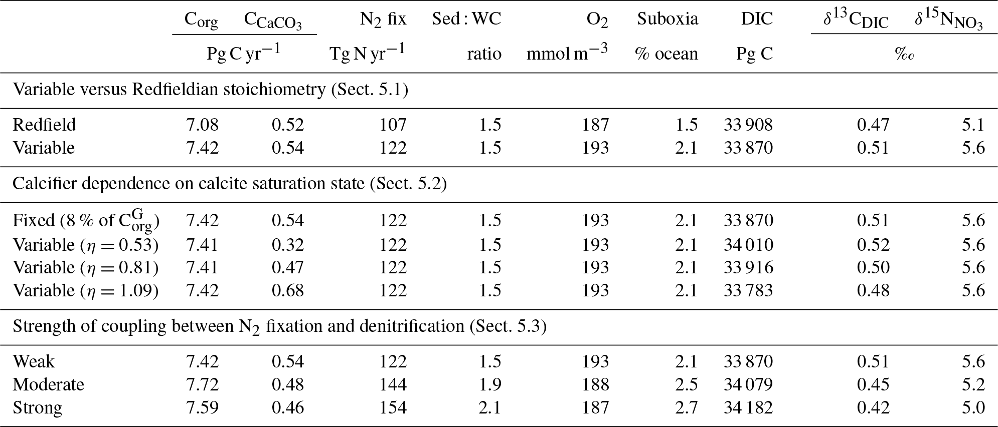
5.1 Variable versus Redfieldian stoichiometry
Enabling variable stoichiometry (see Sect. A3 in the Appendix) of the general phytoplankton group () over a Redfieldian ratio ( ) altered the rate and distribution of organic matter export. Organic matter had more carbon and nitrogen per unit phosphorus in regions with low PO4, such as the Atlantic Ocean (Fig. 11a), which elevated O2 and NO3 demand during oxic and suboxic remineralisation (denitrification), respectively. Lower ratios were produced in eutrophic regions such as the subarctic Pacific, Southern Ocean and tropical zones of upwelling. Overall, global mean C:P increased from the Redfieldian 106:1 to 117:1 and caused an increase in carbon export from 7.6 to 8.0 Pg C yr−1. Approximately 0.1 Pg C yr−1, or 25 % of the increase, was attributed purely to organic carbon export from N2 fixation, which increased from 107 to 122 Tg N yr−1 as higher N:P ratios in the tropics broadened their competitive niche. The total contribution of N2 fixation to the increase in carbon export was likely greater than 25 %, as NO3 also became more available to NO3-limited ecosystems in the lower latitudes (Moore et al., 2013). The increase in carbon export under variable stoichiometry as compared to a Redfieldian ocean was therefore felt largely in the lower latitudes between 40∘ S and 40∘ N (Fig. 11b). Export production decreased poleward of 40∘, particularly in the Southern Ocean, because C:P ratios were lower than the 106:1 Redfield ratio (Fig. 11a).
Distributions of both isotopes were affected by the change in carbon export and the marine nitrogen cycle. Global mean δ13CDIC increased from 0.47 ‰ to 0.51 ‰ and increased from 5.1 ‰ to 5.6 ‰. These are not great changes on the global scale and they had little influence on model–data measures of fit. However, the spatial distribution of these isotopes was significantly altered. Intermediate waters leaving the Southern Ocean were depleted in δ13CDIC by up to 0.1 ‰ and by up to 1 ‰, while the deep ocean, particularly the Pacific, was enriched in both isotopes to a similar degree (Fig. 12). Depletion of both isotopes in waters subducted between 40 and 60∘ S reflected the local loss in export production as a result of lower C:P and N:P ratios, such that biological fractionation was unable to enrich DIC and NO3 in the heavier isotope to the same degree as surface waters travelled north. Enrichment of δ13C in the deep ocean was the result of reduced carbon export in the Antarctic zone due to low C:P ratios, while enrichment of δ15N in the deep ocean was the result of increased tropical production that increased water column denitrification ( =20 ‰). Lower C:P and N:P ratios in both the Antarctic and Subantarctic zones therefore elicited divergent isotope effects in deep and intermediate waters leaving the Southern Ocean.
Meanwhile, each isotope showed a different response in the suboxic zones of the tropics where variable stoichiometry increased the volume of suboxia (O2<10 mmol m−3) by 0.5 %. The increase in water column denitrification caused by the expansion of suboxia increased , while the local increase in carbon export that drove the increase in water column denitrification reduced δ13CDIC in the same waters (Fig. 12). Overall, the increase in low-latitude carbon export caused an expansion of water column suboxia and elicited diverging behaviours in the isotopes, whereby increased and δ13CDIC decreased.
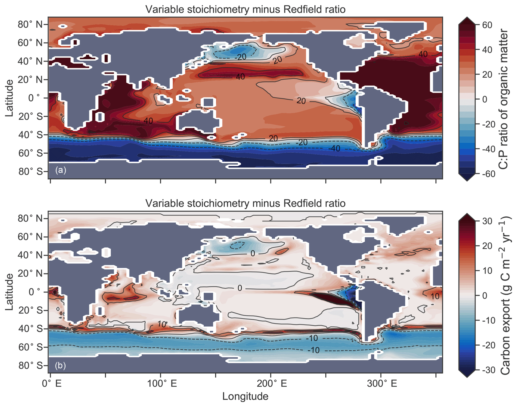
Figure 11Simulated difference in the C:P ratio of exported organic matter due to variable stoichiometry as compared to Redfield stoichiometry (a) and the resulting change in carbon export out of the euphotic zone (b).
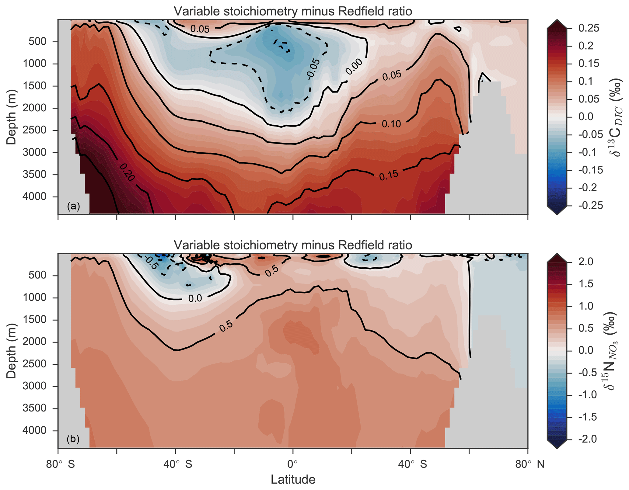
Figure 12Differences in δ13CDIC (a) and (b) as a result of variable stoichiometry as compared to Redfield stoichiometry. Values are zonal means.
5.2 Calcifier dependence on calcite saturation state
The rate of calcification of planktonic foraminifera and coccolithophores is dependent on the calcite saturation state (Zondervan et al., 2001). In previous experiments, the production of CaCO3 was fixed at a rate of 8 % per unit of organic carbon produced in accordance with the modelling study of Yamanaka and Tajika (1996) and produced 0.54 Pg CaCO3 yr−1. Now we investigate how spatial variations in the CaCO3:Corg ratio ( in Eq. A17) affected δ13CDIC and δ13CCib (see Sect. A1.3 in the Appendix). We applied three different values of η to Eq. (A18) to alter the quantity of CaCO3 produced per unit of organic carbon () given the calcite saturation state (Ωca). The η coefficients were 0.53, 0.81 and 1.09. These numbers are equivalent to those in the experiments of Zhang and Cao (2016).
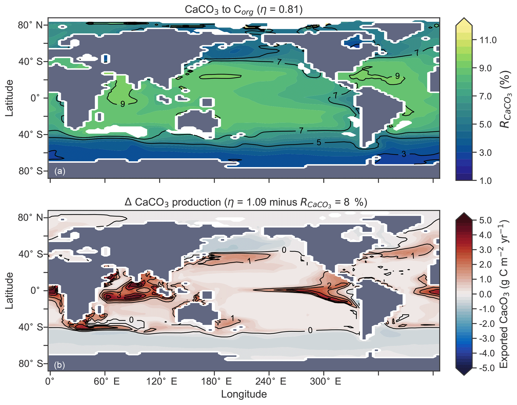
Figure 13Global distribution of CaCO3 export as a percentage of organic carbon (Corg) export (a) and the change in the CaCO3 production field as a result of making CaCO3 production dependent on calcite saturation state (η=1.09) compared to when it was a fixed 8 % of Corg (b). Areas where export production does not occur due to severely nutrient limited conditions are masked out.
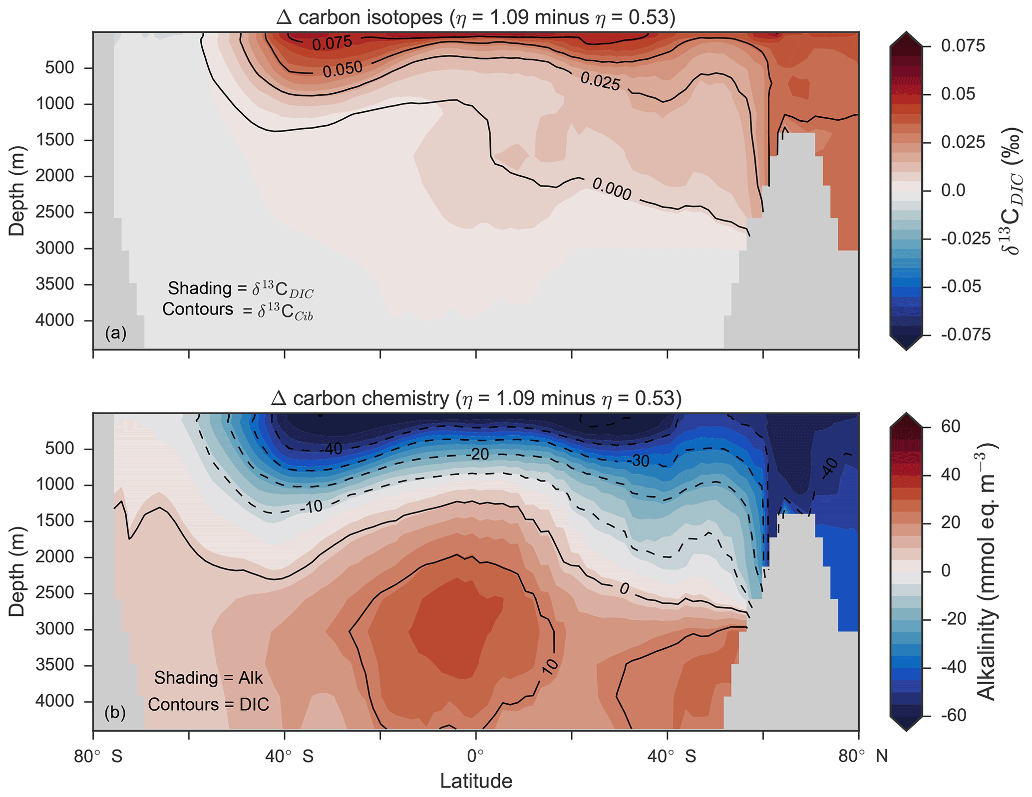
Figure 14Changes in the distribution of carbon isotopes (δ13CDIC and δ13CCib; a) and carbon chemistry (dissolved inorganic carbon and alkalinity; b) as a result of increasing CaCO3 production in surface waters between 40∘ S and 40∘ N.
Mean was 4.5 %, 6.6 % and 9.5 %, and annual CaCO3 production was 0.32, 0.47 and 0.68 Pg CaCO3 yr−1 in the three experiments. Although different in total CaCO3 production, the three experiments shared the same spatial patterns. Low-latitude waters were high in , particularly the oligotrophic subtropical gyres, while high latitudes were low, particularly the Antarctic zone where mixing of old waters into the surface depressed the calcite saturation state (Fig. 13). These regional patterns in therefore had the largest effect in areas of high export production. Productive, high-latitude areas like the Southern Ocean, subpolar Pacific and North Atlantic waters all produced less CaCO3 when compared to an enforced 8 % rain ratio, while CaCO3 production between 40∘ S and 40∘ N relative to a fixed of 8 % was dependent on η. The highest η coefficient of 1.09 achieved greater export of CaCO3 in the mid- to lower-latitude regions of high export production (Fig. 13). The consequence of increasing CaCO3 production in the middle–lower latitudes was a loss of upper ocean alkalinity, subsequent outgassing of CO2 and losses in the DIC inventory. Losses in global DIC were 95 and 130 Pg C as increased from % (Table 6), equivalent to one-fifth of the glacial increase in oceanic carbon (Ciais et al., 2011).
Despite the significant changes associated with the implementation of Ωca-dependent CaCO3 production, effects were negligible on both δ13CDIC and δ13CCib. Global mean δ13CDIC was 0.51 ‰, when was fixed at 8 %, and this changed to 0.52 ‰, 0.50 ‰ and 0.48 ‰ under η coefficients of 0.53, 0.81 and 1.09 (Table 6). Likewise, global mean δ13CCib was 0.59 ‰, when was fixed at 8 %, and this changed to 0.60 ‰, 0.58 ‰ and 0.55 ‰. Minimal change in δ13CCib indicated minimal change in the concentration (see Eq. 21), which varied by ≤2 mmol m−3 between experiments. Visual inspection of the change in δ13CDIC and δ13CCib distributions showed an enrichment of these isotopes in the upper ocean north of 40∘ S. Subsequent increases in η, which increased low-latitude CaCO3 production, magnified the enrichment. Enrichment of δ13CDIC and δ13CCib was caused by outgassing of CO2 as surface alkalinity decreased in response to greater CaCO3 production (Fig. 14). The change, however, was at most 0.1 ‰, which lies well within 1 standard deviation of variability known in the proxy data (Schmittner et al., 2017). We therefore find little scope for recognising even large variations in global CaCO3 production (0.32 to 0.68 Pg CaCO3 yr−1) in the signature of carbon isotopes despite considerable effects on the oceanic inventory of DIC.
However, we stress that version 1.0 of CSIRO Mk3L-COAL does not include CaCO3 burial or dissolution from the sediments according the calcite saturation state of overlying water (Boudreau, 2013). To neglect ocean–sediment CaCO3 cycling is to neglect of an important aspect of the global carbon cycle active on millennial timescales (Sigman et al., 2010). Changes in CaCO3 burial and dissolution could have a non-negligible effect on δ13C through altering whole ocean alkalinity and thereby air–sea gas exchange of CO2, which would in turn affect surface δ13C as we have seen. While we do not address these effects here, we aim to do so in upcoming versions of the model equipped with carbon compensation dynamics.
5.3 Strength of coupling between N2 fixation and denitrification
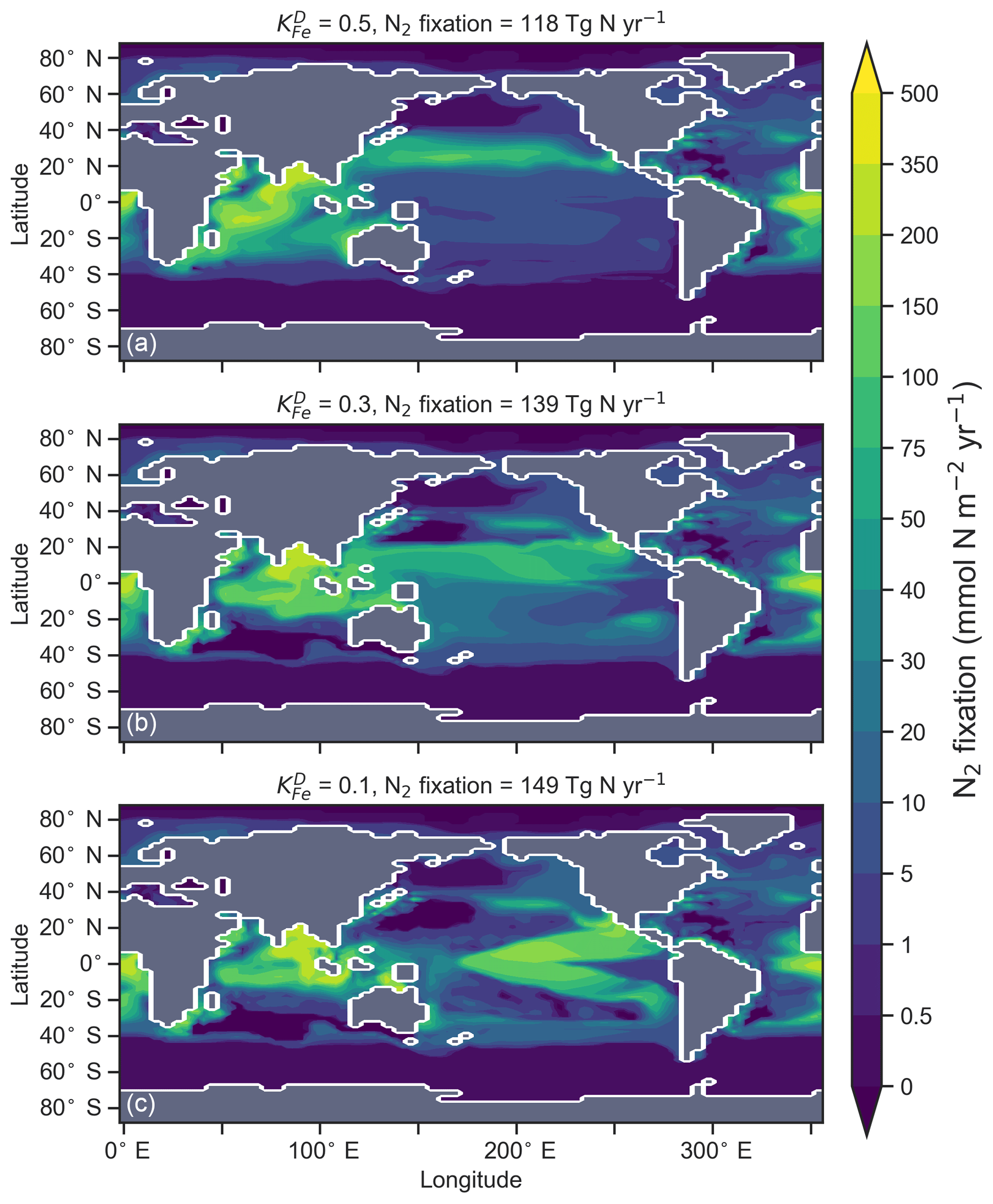
The degree to which N2 fixers are spatially coupled to the tropical denitrification zones is controlled by altering the degree to which N2 fixers are limited by iron () in Eq. (A12) (see Sect. A1.2 in the Appendix). Decreasing ensures that N2 fixation becomes less dependent on iron supply and as such is released from regions of high aeolian deposition, such as the North Atlantic, to inhabit areas of low NO3:PO4 ratios. Areas of low NO3:PO4 exist in the tropics proximal to water column denitrification zones. Releasing N2 fixers from Fe limitation therefore increases the spatial coupling between N2 fixation and water column denitrification and increases the global rate of N2 fixation.

Figure 16Change in caused by a stronger coupling between N2 fixation and tropical regions of low NO3:PO4 concentrations (i.e. tropical upwelling zones with active water column denitrification). Panel (a) shows the global zonal mean change, while panel (b) shows the average change in the euphotic zone, here defined as the top 100 m. Areas with very low NO3 (<0.1 mmol m−3) are masked out.
We steadily decreased iron limitation () to increase the strength of spatial coupling between N2 fixers and the tropical denitrification zones (Fig. 15). As N2 fixers coupled more strongly to regions of low NO3:PO4, the rate of N2 fixation increased from 122 to 144 to 154 Tg N yr−1 (Table 6). An expansion of suboxia from 2.1 % to 2.5 % to 2.7 % of global ocean volume in the tropics accompanied the increase in N2 fixation, as did a decrease in global mean δ13CDIC of 0.06 ‰ and 0.1 ‰, since greater rates of N2 fixation stimulated tropical export production. Due to the expansion of the already large suboxic zones, which occurred in both horizontal and vertical directions, the amount of organic carbon that reached tropical sediments (20∘ S to 20∘ N) increased from 0.35 to 0.46 to 0.51 Pg C yr−1.
The overarching consequence for due to an expansion of the suboxic zones was an increase in the sedimentary to water column denitrification ratio from 1.5 to 1.9 to 2.2, which decreased mean from 5.6 ‰ to 5.2 ‰ to 5.0 ‰ (Table 6). The increase in N2 fixation () and sedimentary denitrification () in the tropics was felt globally for (Fig. 16). Lower by 0.5 ‰ and 0.9 ‰ permeated water columns in the Southern Ocean and tropics, respectively. Meanwhile, was up to 10 ‰ lower in surface waters of the tropical and subtropical Pacific, which is where the greatest increase in N2 fixation and sedimentary denitrification occurred. The dramatic reduction in surface was subsequently conveyed to the sediments as δ15Norg±1 ‰–2 ‰.
These simple experiments demonstrate that the insights garnered from sedimentary records of δ15N are open to multiple lines of interpretation. An expansion of the suboxic zones, normally associated with an increase in (Galbraith et al., 2013), could instead cause a decrease in if more organic matter reached the sediments to stimulate sedimentary denitrification. There is good evidence that the suboxic zones might have undergone a vertical expansion (Hoogakker et al., 2018) and that more organic matter reached the tropical sediments under glacial conditions (Cartapanis et al., 2016). The glacial decrease in bulk δ15Norg recorded in the eastern tropical Pacific (Ganeshram et al., 1995; Liu et al., 2008) therefore does not necessarily mean a decrease in suboxia. Rather, our experiments show that lower δ15Norg might also be caused by an increase in local N2 fixation and sedimentary denitrification. The decrease in associated with more sedimentary denitrification and local N2 fixation demonstrates the complexity of interpreting sedimentary δ15Norg records in the lower latitudes.
The stable isotopes of carbon (δ13C) and nitrogen (δ15N) are proxies that have been fundamental for understanding the ocean. We have included both isotopes into the ocean component of an Earth system model, CSIRO Mk3L-COAL, to enable future studies with the capability for direct model–proxy data comparisons. We detailed how these isotopes are simulated, how to conduct model–data comparisons using both water column and sedimentary data and some basic assessment of changes caused by altered ecosystem functioning. We made three overall findings. First, CSIRO Mk3L-COAL performs well alongside a number of isotope-enabled global ocean GCMs. Second, alteration of δ13C during formation of foraminiferal calcite does not jeopardise simple one-to-one comparisons with simulated δ13C of DIC, while diagenetic alteration of bulk organic δ15N during early burial must be accounted for in model–data comparisons. Third, changes in how marine ecosystems function can have significant and complex effects on δ13C and δ15N. Our idealised experiments hence showed that the interpretation of palaeoceanographic records may suffer from multiple lines of interpretation, particularly records from the lower latitudes where multiple processes imprint on the isotopic signatures laid down in sediments. Future work will involve palaeoceanographic simulations of CSIRO Mk3L-COAL that seek to understand how the oceanic carbon and nitrogen cycles respond to and influence important climate transitions.
All model output is provided for download on Australia's National Computing Infrastructure (NCI) at https://geonetwork.nci.org.au/geonetwork/srv/eng/catalog.search\#/metadata/f3048_7378_3224_4737 (last access: 12 April 2019) and is citable with https://doi.org/10.25914/5c6643f64446c (Buchanan et al., 2019). Nitrogen isotope data are available by request to Dario M. Marconi and Daniel M. Sigman at Princeton University. LOVECLIM data are freely available for download at https://doi.org/10.4225/41/58192cb8bff06 (Menviel et al., 2017b). UVic-MOBI data were provided by Christopher Somes, PISCES data by Laurent Bopp, iCESM-high data from Simon Yang and iCESM-low data by Alexandra Jahn.
The source code for CSIRO Mk3L-COAL is shared via a repository located at http://svn.tpac.org.au/repos/CSIRO_Mk3L/branches/CSIRO_Mk3L-COAL/ (last access: 12 April 2019). Access to the repository may be obtained by following the instructions at https://www.tpac.org.au/csiro-mk3l-access-request/ (last access: 12 April 2019). Access to the source code is subject to a bespoke license that does not permit commercial usage but is otherwise unrestricted. An “out-of-the-box” run directory is also available for download with all files required to run the model in the configuration used in this study, although users will need to modify the runscript according to their computing infrastructure.
A1 Export production
A1.1 General phytoplankton group (G)
The production of organic matter by the general phytoplankton group () is measured in units of mmol phosphorus (P) m−3 d−1 and is dependent on temperature (T), nutrients (PO4, NO3 and Fe) and irradiance (I):
In the example above, SE:P converts growth rates in units of d−1 to mmol PO4 m−3 d−1. SE:P conceptually represents the export to production ratio, and for simplicity we assume it does not change. μ(T) is the temperature-dependent maximum daily growth rate of phytoplankton (doubling per day), as defined by Eppley (1972). The light limitation term (F(I)) is the productivity versus irradiance equation used to describe phytoplankton growth defined by Clementson et al. (1998) and is dependent on I, the daily averaged shortwave incident radiation (W m−2), α, the initial slope of the productivity versus radiance curve (d−1 (W m−2)−1) and PAR, the fraction of shortwave radiation that is photosynthetically active.
The nutrient limitation terms (, and ) may be calculated in two ways.
If the option for static nutrient limitation is true, then Michaelis–Menten kinetics (Dugdale, 1967) is used:
Half-saturation coefficients () show a large range across phytoplankton species (e.g. Timmermans et al., 2004), and so for simplicity, we set mmol PO4 m−3 (Smith, 1982), mmol NO3 m−3 (Eppley et al., 1969; Carpenter and Guillard, 1971) and µmol Fe m−3 (Timmermans et al., 2001).
If the option for variable nutrient limitation is true (default), then optimal uptake kinetics (Smith et al., 2009) is used:
Optimal uptake kinetics varies the two terms in the denominator of the Michaelis–Menten form according to the availability of nutrients. It therefore accounts for different phytoplankton communities with different abilities for nutrient uptake and does so using the fA term. The V∕A term represents the maximum potential nutrient uptake, V, over the cellular affinity for that nutrient, A, and is set at 0.1.
A1.2 Diazotrophs (D; N2 fixers)
Organic matter produced by diazotrophs () is also measured in units of mmol phosphorus (P) m−3 d−1 and is calculated in the same form of Eq. (A1), but using the maximum growth rate μ(T)D of Kriest and Oschlies (2015), notable changes in the limitation terms and minimum thresholds that ensure the nitrogen fixation occurs everywhere in the ocean, except under sea ice. is calculated via
The half-saturation values for PO4 and Fe limitation are set at 0.1 mmol m−1 and 0.5 µmol m−1, respectively, in the default parameterisation. The motivation for making N2 fixers strongly limited by Fe was the high cellular requirements of Fe for diazotrophy (see Sohm et al., 2011, and references therein). A dependency on light is omitted from the limitation term when is produced. The omission of light is justified by its strong correlation with sea surface temperature (Luo et al., 2014) and its negligible effect on nitrogen fixation in the Atlantic Ocean (McGillicuddy, 2014). Finally, the fractional area coverage of sea ice (ico) is included to ensure that cold water N2 fixation (Sipler et al., 2017) does not occur under ice, since a light dependency is omitted.
A1.3 Calcifiers
The calcifying group produces calcium carbonate (CaCO3) in units of mmol carbon (C) m−3 d−1. The production of CaCO3 is always a proportion of the organic carbon export of the general phytoplankton group (), according to
The ratio of CaCO3 to () can be calculated in two ways.
If the option for fixed is true (default), then is set to 0.08 as informed by the experiments of Yamanaka and Tajika (1996). The production of CaCO3 is thus 8 % of everywhere.
If the option for variable is true, then varies as a function of the saturation state of calcite (Ωca) according to Ridgwell et al. (2007), where
The exponent (η) is easily modified consistent with the parameterisations of Zhang and Cao (2016) and controls the rate of CaCO3 production at a given value of Ωca.
A2 Remineralisation
A2.1 General phytoplankton group (G)
Organic matter produced by the general phytoplankton group (in units of phosphorus: ) at the surface is instantaneously remineralised each time step at depth levels beneath the euphotic zone using a power law scaled to depth (Martin et al., 1987). This power law defines the concentration of organic matter remaining at a given depth () as a function of organic matter at the surface () and depth itself (z). Its form is as follows:
where zrem in the denominator represents the depth at which remineralisation begins and is set to be 100 m everywhere. The OBGCM therefore does not consider sinking speeds or an interaction between organic matter and physical mixing. However, variations in the b exponent affect the steepness of the curve, thereby emulating sinking speeds and affecting the transfer and release of nutrients from the surface to the deep ocean.
Remineralisation of through the water column is therefore dependent on the exponent b value in Eq. (A19). The b exponent is calculated in two ways.
If the option for static remineralisation is true, then b is set to −0.858 according to Martin et al. (1987).
If the option for variable remineralisation is true (default), then b is dependent on the component fraction of picoplankton (Fpico) in the ecosystem. The Fpico shows a strong inverse relationship to the transfer efficiency (Teff) of organic matter from beneath the euphotic zone to 1000 m depth (Weber et al., 2016). Because Fpico is not explicitly simulated in OBGCM, we estimate Fpico from the export production field in units of carbon (), calculate Teff using the parameterisation of Weber et al. (2016) and subsequently calculate the b exponent:
A2.2 Diazotrophs (D)
Remineralisation of diazotrophs () is calculated in the same way as the general phytoplankton group (), with the exception that the depth at which remineralisation occurs is raised from 100 to 25 m in Eq. (A19). This alteration emulates the release of NO3 from N2 fixers well within the euphotic zone, which in some cases can exceed the physical supply from below (Capone et al., 2005). Release of their N- and C-rich organic matter (see stoichiometry Sect. A3.2) therefore occurs higher in the water column than the general phytoplankton group.
A2.3 Suboxic environments
The remineralisation of and will typically require O2 to be removed, except for in regions where oxygen concentrations are less than a particular threshold (Den), which is set to 7.5 mmol O2 m−3 and represents the onset of suboxia. In these regions, the remineralisation of organic matter begins to consume NO3 via the process of denitrification. We calculate the fraction of organic matter that is remineralised by denitrification (Fden) via
such that Fden rises and plateaus at 100 % in a sigmoidal function as O2 is depleted from 7.5 to 0 mmol m−3.
Following this, the strength of denitrification is reduced if the ambient concentration of NO3 is deemed to be limiting. Denitrification within the modern oxygen minimum zones only depletes NO3 towards concentrations between 15 and 40 mmol m−3 (Codispoti and Richards, 1976; Voss et al., 2001). Without an additional constraint that weakens denitrification as NO3 is drawn down, here defined as rden, NO3 concentrations quickly go to zero in simulated suboxic zones (Schmittner et al., 2008). We weaken denitrification by prescribing a lower bound at which NO3 can no longer be consumed via denitrification, , which is set at 30 mmol NO3 m−3.
Fden is therefore reduced if NO3 is deemed to be limiting and subsequently applied against both and to get the proportion of organic matter to be remineralised by O2 and NO3.
If the availability of O2 and NO3 is insufficient to remineralise all the organic matter at a given depth level, z, then the unremineralised organic matter will pass into the next depth level. Unremineralised organic matter will continue to pass into lower depth levels until the final depth level is reached, at which point all organic matter is remineralised by either water column or sedimentary processes. This version of CSIRO Mk3L-COAL does not consider burial of organic matter.
A2.4 Calcifiers
The dissolution of CaCO3 is calculated using an e-folding depth-dependent decay, where the amount of CaCO3 at a given depth z is defined by
where zdis represents the depth at which e−1 of CaCO3 (∼0.37) produced at the surface remains undissolved.
Calcifiers are not susceptible to oxygen-limited remineralisation or the concentration of carbonate ion because the dissolution of CaCO3 depends solely on this depth-dependent decay. All CaCO3 reaching the final depth level is remineralised without considering burial. Future work will include a full representation of carbonate compensation.
A3 Stoichiometry
The elemental constitution, or stoichiometry, of organic matter affects the biogeochemistry of the water column through uptake (production) and release (remineralisation). The general phytoplankton group and diazotrophs both affect carbon chemistry, O2 and nutrients (PO4, NO3 and Fe), while the calcifiers only affect carbon chemistry tracers (DIC, DI13C and ALK).
Alkalinity ratios for both the general and nitrogen-fixing groups are the negative of the N:P ratio, such that for a loss of 1 mmol of NO3, alkalinity will increase at 1 mmol eq m−3 (Wolf-Gladrow et al., 2007).
A3.1 General phytoplankton group (G)
The stoichiometry of the general phytoplankton group is calculated in two ways.
If the option for static stoichiometry is true, then the ratio is set according to the Redfield ratio of (Redfield et al., 1937).
If the option for variable stoichiometry is true (default), then the ratio of is made dependent on the ambient nutrient concentration according to Galbraith and Martiny (2015):
Thus, the stoichiometry of varies across the ocean according to the nutrient concentration, and the uptake and release of carbon, nutrients and oxygen (see Sect. A3.4) are dependent on the concentration of surface PO4 and NO3. The ratio of iron to phosphorus (Fe:P) remains fixed at 0.00032, such that 0.32 µmol of Fe is consumed per mmol of PO4. We chose to maintain a fixed Fe:P ratio because phytoplankton communities from subtropical to Antarctic waters appear to show similar iron content (Boyd et al., 2015), despite changes in . However, the ratio of does change as a result of varying ratios, with higher C:Fe in oligotrophic environments and lower C:Fe in eutrophic regions.
A3.2 Diazotrophs (D)
The stoichiometry of diazotrophs is fixed at a ratio of , which represents values reported in the literature (Kustka et al., 2003; Karl and Letelier, 2008; Mills and Arrigo, 2010). Diazotrophs do not consume NO3; rather, they consume N2, which is assumed to be of unlimited supply, and release NO3 during remineralisation.
A3.3 Calcifiers
Calcifying organisms produce CaCO3, which includes DIC, DI13C and ALK, and these tracers are consumed and released at a ratio of , respectively, relative to organic carbon. Thus, the ratio of relative to each unit of phosphorus consumed by the general phytoplankton group is equal to the rain ratio of CaCO3 to organic phosphorus multiplied by . This group has no effect on nutrient tracers or oxygen values.
A3.4 Stoichiometry of remineralisation
The requirements for oxygen () and nitrate () during oxic and suboxic remineralisation, respectively, are calculated from the ratios of organic matter via the equations of Paulmier et al. (2009). Additional knowledge of the hydrogen and oxygen content of the organic matter is also required to calculate and . However, the hydrogen and oxygen content of phytoplankton depends strongly on the proportions of lipids, carbohydrates and proteins that constitute the cell. As there is no empirical model for predicting these physiological components based on environmental variables, we continue Redfield's legacy by assuming that all organic matter is a carbohydrate of the form CH2O. Future work, however, should address this obvious bias.
To calculate and , we therefore need to first calculate the amount of hydrogen and oxygen in organic matter via
Once a ratio for organic matter is known, we calculate and in units of mmol m−3 P−1 using the equations of Paulmier et al. (2009):
The calculation of accounts for the oxygen that is also needed to oxidise ammonium to nitrate.
From these calculations, we find the following requirements of oxic and suboxic remineralisation, assuming the static stoichiometry option for the general phytoplankton group:
These numbers change dynamically alongside ratios when the stoichiometry of organic matter is allowed to vary.
A4 Sedimentary processes
The remineralisation of organic matter within the sediments is provided as an option in the OBGCM. Sedimentary denitrification, and its slight preference for the light isotopes of fixed nitrogen ( =3 ‰), is an important component of the marine nitrogen cycle and its isotopes. It acts as an additional sink of NO3 and reduces the δ15N value of the global ocean by offsetting the strong fractionation of water column denitrification ( =20 ‰).
If sedimentary processes are active, the empirical model of Bohlen et al. (2012) is used to estimate the rate of sedimentary denitrification, where the removal of NO3 is dependent on the rate of particulate organic carbon ( + ) arriving at the sediments and the ambient concentrations of oxygen and nitrate. In the following, we assume that the concentrations of NO3 and O2 that are available in the sediments are two-thirds of the concentration in the overlying water column based on observations of transport across the diffusive boundary layer (Gundersen and Jorgensen, 1990).
In the example above, both the α and β values were halved from the values of Bohlen et al. (2012) to raise global mean NO3 concentrations and lower the sedimentary to water column denitrification ratio to between 1 and 2. If NO3 is not available, the remaining organic matter is remineralised using oxygen if the environment is sufficiently oxygenated. An additional limitation is set for sediments underlying hypoxic waters (O2<40 mmol m−3), where oxic remineralisation is weakened towards zero according to a hyperbolic tangent function . If oxygen is also limiting, the remaining organic matter is remineralised via sulfate reduction. As sulfate is not explicitly simulated, we assumed that sulfate is always available to account for the remaining organic matter.
Thus, sedimentary denitrification is heavily dependent on the rate of organic matter arriving at the sediments. However, a large amount of sedimentary remineralisation is not captured using only these parameterisations because the coarse resolution of the OGCM enables it to resolve only the largest continental shelves, such as the shallow Indonesian seas. Many small areas of raised bathymetry in pelagic environments are also unresolved by the OGCM. To address this insufficiency and increase the global rate of sedimentation and sedimentary denitrification, we coupled a subgrid-scale bathymetry to the coarse-resolution OGCM following the methodology of Somes et al. (2013) using the Earth topography 5 min grid (ETOPO5) 1/12∘ dataset. For each latitude-by-longitude grid point, we calculated the fraction of area that would be represented by shallower levels in the OGCM if this finer-resolution bathymetry were used. At each depth level above the deepest level, the fractional area represented by sediments on the subgrid-scale bathymetry can be used to remineralise all forms of exported matter (, and CaCO3) via sedimentary processes.
Also following the methodology of Somes et al. (2013), we included an option to amplify sedimentary denitrification in the upper 250 m to account for narrow continental shelves that are not resolved by the OGCM. Narrow shelves experience strong rates of upwelling and productivity, and hence high rates of sedimentary denitrification (Gruber and Sarmiento, 1997). To amplify shallow rates of sedimentary denitrification, we included an optional acceleration factor (Γsed), set to 3.0 in the default parameterisation, dependent on the total fraction of shallower depths not covered by the subgrid-scale bathymetry:
For those grids with a low fraction covered by the subgrid-scale bathymetry (Fsgb), the amplification of sedimentary denitrification is therefore greatest.
Default parameters for the marine ecosystem component of CSIRO Mk3L-COAL are outlined in Tables B1, B2 and B3. The values presented in these tables are required as input when running the ocean model.
Table B1Parameter values controlling export production in the ecosystem component of the CSIRO Mk3L-COAL ocean model. Default settings: Michaelis–Menten == False, Optimal Uptake == True, fix == True and Vary CaCO3 == False.
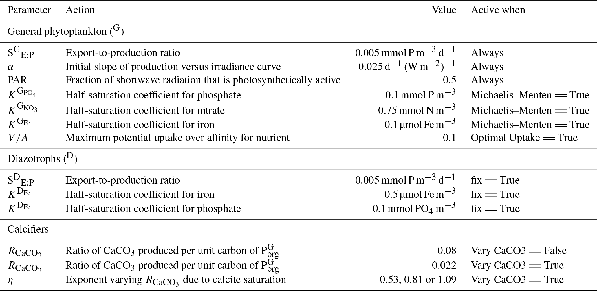
Table B2Parameter values controlling remineralisation in the ecosystem component of the CSIRO Mk3L-COAL ocean model. Default settings: ReminPico == True, fix == True, den == True and sedfluxes == True.
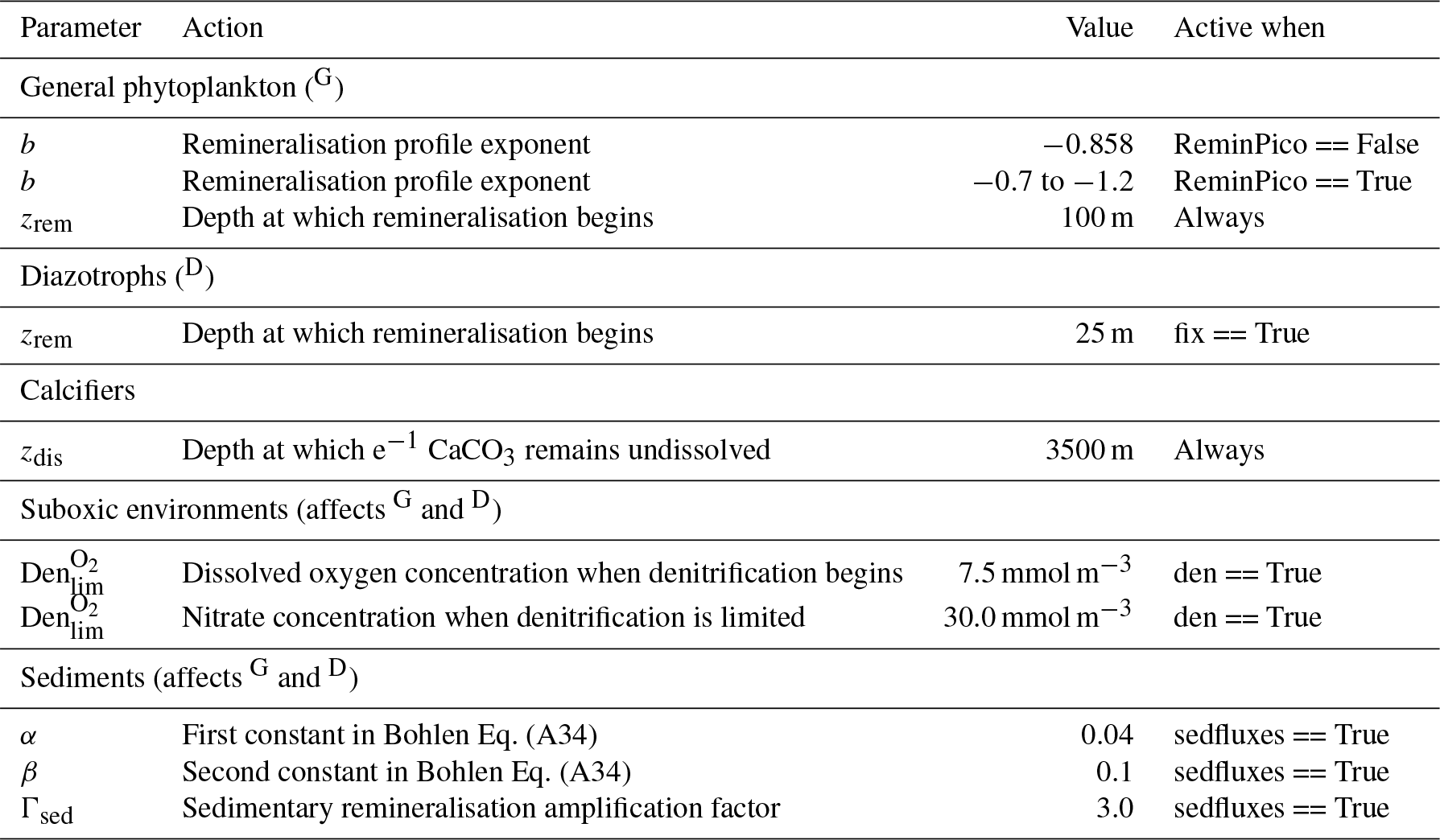
Table B3Parameter values controlling stoichiometry in the ecosystem component of the CSIRO Mk3L-COAL ocean model. Default settings: Vary Stoich == True, Vary frac13 == False and fix == True.

The supplement related to this article is available online at: https://doi.org/10.5194/gmd-12-1491-2019-supplement.
PJB designed the study, undertook model development, ran the experiments, analysed model output and wrote the manuscript. RJM designed the study, provided instruction on development, aided in analysis and edited the manuscript. ZC designed the study, aided in analysis and edited the manuscript. SJP aided in model development and edited the manuscript. NLB aided in interpretation of results and edited the manuscript.
The authors declare that there is no conflict of interest.
The Australian Research Council's Centre of Excellence for Climate System Science and the Tasmanian Partnership for Advanced Computing (TPAC) were instrumental for this research. This research was supported under the Australian Research Council's Special Research Initiative for the Antarctic Gateway Partnership (project ID SR140300001). The authors wish to acknowledge the use of the Ferret programme for the analysis undertaken in this work. Ferret is a product of NOAA's Pacific Marine Environmental Laboratory (information is available at http://ferret.pmel.noaa.gov/Ferret/, last access: 12 April 2019). The Matplotlib package (Hunter, 2007) and the cmocean package (Thyng et al., 2016) were used for producing the figures. We are indebted to Kristen Karsh, Daniel Sigman, Dario Marconi and Eric Raes for discussions that focussed this work. Special thanks are given to Christopher Somes for correspondence in some development steps and revisions that improved the manuscript. Finally, the lead author is indebted to an Australian Fulbright postgraduate scholarship, which supported him at the Princeton Geosciences department during the writing of the manuscript.
This paper was edited by Andrew Yool and reviewed by Christopher Somes and two anonymous referees.
Altabet, M. A. and Francois, R.: Nitrogen isotope biogeochemistry of the Antarctic Polar Frontal Zone at 170 degrees W, Deep-Sea Res. Pt. II, 48, 4247–4273, https://doi.org/10.1016/S0967-0645(01)00088-1, 2001. a, b
Bohlen, L., Dale, A. W., and Wallmann, K.: Simple transfer functions for calculating benthic fixed nitrogen losses and regeneration ratios in global biogeochemical models, Global Biogeochem. Cy., 26, GB3029, https://doi.org/10.1029/2011GB004198, 2012. a, b
Boudreau, B. P.: Carbonate dissolution rates at the deep ocean floor, Geophys. Res. Lett., 40, 744–748, https://doi.org/10.1029/2012GL054231, 2013. a
Boyd, P. W., Strzepek, R. F., Ellwood, M. J., Hutchins, D. A., Nodder, S. D., Twining, B. S., and Wilhelm, S. W.: Why are biotic iron pools uniform across high- and low-iron pelagic ecosystems?, Global Biogeochem. Cy., 29, 1028–1043, https://doi.org/10.1002/2014GB005014, 2015. a
Brandes, J. A. and Devol, A. H.: A global marine-fixed nitrogen isotopic budget: Implications for Holocene nitrogen cycling, Global Biogeochem. Cy., 16, 67–1–67–14, https://doi.org/10.1029/2001GB001856, 2002. a, b, c
Buchanan, P., Matear, R., Chase, Z., Phipps, S., and Bindoff, N.: Dynamic Biological Functioning Important for Simulating and Stabilizing Ocean Biogeochemistry, Global Biogeochem. Cy., 32, 565–593, https://doi.org/10.1002/2017GB005753, 2018. a, b
Buchanan, P. J., Matear, R. J., Lenton, A., Phipps, S. J., Chase, Z., and Etheridge, D. M.: The simulated climate of the Last Glacial Maximum and insights into the global marine carbon cycle, Clim. Past, 12, 2271–2295, https://doi.org/10.5194/cp-12-2271-2016, 2016. a, b
Buchanan, P. J., Matear, R. J., Chase, Z., Phipps, S. J., and Bindoff, N. L.: Oceanic carbon-13 and nitrogen-15 isotopes simulated by CSIRO Mk3L-COAL version 1.0, https://doi.org/10.25914/5c6643f64446c, 2019. a
Capone, D. G., Burns, J. A., Montoya, J. P., Subramaniam, A., Mahaffey, C., Gunderson, T., Michaels, A. F., and Carpenter, E. J.: Nitrogen fixation by Trichodesmium spp.: An important source of new nitrogen to the tropical and subtropical North Atlantic Ocean, Global Biogeochem. Cy., 19, GB2024, https://doi.org/10.1029/2004GB002331, 2005. a
Carpenter, E. J. and Guillard, R. R. L.: Intraspecific differences in nitrate half-saturation constants for three species of marine phytoplankton, Ecology, 52, 183–185, 1971. a
Carpenter, E. J., Harvey, H. R., Brian, F., and Capone, D. G.: Biogeochemical tracers of the marine cyanobacterium Trichodesmium, Deep-Sea Res. Pt. I, 44, 27–38, https://doi.org/10.1016/S0967-0637(96)00091-X, 1997. a
Cartapanis, O., Bianchi, D., Jaccard, S. L., and Galbraith, E. D.: Global pulses of organic carbon burial in deep-sea sediments during glacial maxima, Nat. Commun., 7, 1–7, https://doi.org/10.1038/ncomms10796, 2016. a
Ciais, P., Tagliabue, A., Cuntz, M., Bopp, L., Scholze, M., Hoffmann, G., Lourantou, A., Harrison, S. P., Prentice, I. C., Kelley, D. I., Koven, C., and Piao, S. L.: Large inert carbon pool in the terrestrial biosphere during the Last Glacial Maximum, Nat. Geosci., 5, 74–79, https://doi.org/10.1038/ngeo1324, 2011. a
Clementson, L., Parslow, J., Griffiths, F., Lyne, V., Mackey, D., Harris, G., McKenzie, D., Bonham, P., Rathbone, C., and Rintoul, S.: Controls on phytoplankton production in the Australasian sector of the subtropical convergence, Deep-Sea Res. Pt. I, 45, 1627–1661, https://doi.org/10.1016/S0967-0637(98)00035-1, 1998. a
Cline, J. D. and Kaplan, I. R.: Isotopic fractionation of dissolved nitrate during denitrification in the eastern tropical north pacific ocean, Mar. Chem., 3, 271–299, https://doi.org/10.1016/0304-4203(75)90009-2, 1975. a
Codispoti, L. A. and Richards, F. A.: An analysis of the horizontal regime of denitrification in the eastern tropical North Pacific, Limnol. Oceanogr., 21, 379–388, https://doi.org/10.4319/lo.1976.21.3.0379, 1976. a
Craig, H.: Isotopic standards for carbon and oxygen and correction factors for mass-spectrometric analysis of carbon dioxide, Geochim. Cosmochim. Ac., 12, 133–149, https://doi.org/10.1016/0016-7037(57)90024-8, 1957. a
Dugdale, R. C.: Nutrient limitation in the Sea: Dynamics, identification, and significance, Limnol. Oceanogr., 12, 685–695, 1967. a
Duteil, O., Koeve, W., Oschlies, A., Bianchi, D., Galbraith, E., Kriest, I., and Matear, R.: A novel estimate of ocean oxygen utilisation points to a reduced rate of respiration in the ocean interior, Biogeosciences, 10, 7723–7738, https://doi.org/10.5194/bg-10-7723-2013, 2013. a
Eide, M., Olsen, A., Ninnemann, U. S., and Johannessen, T.: A global ocean climatology of preindustrial and modern ocean δ13C, Global Biogeochem. Cy., 31, 515–534, https://doi.org/10.1002/2016GB005473, 2017. a, b, c, d, e, f, g
Eppley, R. W.: Temperature and phytoplankton growth in the sea, Fish. B.-NOAA, 70, 1063–1085, 1972. a
Eppley, R. W., Rogers, J. N., and Mccarthy, J. J.: Half-saturation constants for uptake of nitrate and ammonium by marine phytoplankton, Limnol. Oceanogr., 14, 912–920, https://doi.org/10.4319/lo.1969.14.6.0912, 1969. a
Freing, A., Wallace, D. W. R., and Bange, H. W.: Global oceanic production of nitrous oxide, Philos. T. R. Soc. B, 367, 1245–1255, https://doi.org/10.1098/rstb.2011.0360, 2012. a
Friedli, H., Lötscher, H., Oeschger, H., Siegenthaler, U., and Stauffer, B.: Ice core record of the 13C/12C ratio of atmospheric CO2 in the past two centuries, Nature, 324, 237–238, https://doi.org/10.1038/324237a0, 1986. a
Galbraith, E. D. and Martiny, A. C.: A simple nutrient-dependence mechanism for predicting the stoichiometry of marine ecosystems, P. Natl. Acad. Sci. USA, 112, 201423917, https://doi.org/10.1073/pnas.1423917112, 2015. a
Galbraith, E. D., Kienast, M., Albuquerque, A. L., Altabet, M. A., Batista, F., Bianchi, D., Calvert, S. E., Contreras, S., Crosta, X., De Pol-Holz, R., Dubois, N., Etourneau, J., Francois, R., Hsu, T. C., Ivanochko, T., Jaccard, S. L., Kao, S. J., Kiefer, T., Kienast, S., Lehmann, M. F., Martinez, P., McCarthy, M., Meckler, A. N., Mix, A., Möbius, J., Pedersen, T. F., Pichevin, L., Quan, T. M., Robinson, R. S., Ryabenko, E., Schmittner, A., Schneider, R., Schneider-Mor, A., Shigemitsu, M., Sinclair, D., Somes, C., Studer, A. S., Tesdal, J. E., Thunell, R., and Terence Yang, J.: The acceleration of oceanic denitrification during deglacial warming, Nat. Geosci., 6, 579–584, https://doi.org/10.1038/ngeo1832, 2013. a, b
Ganeshram, R. S., Pedersen, T. F., Calvert, S. E., and Murray, J. W.: Large changes in oceanic nutrient inventories from glacial to interglacial periods, Nature, 376, 755–758, https://doi.org/10.1038/376755a0, 1995. a, b, c
Gruber, N. and Sarmiento, J. L.: Global patterns of marine nitrogen fixation and denitrification, Global Biogeochem. Cy., 11, 235–266, https://doi.org/10.1029/97GB00077, 1997. a
Gundersen, J. K. and Jorgensen, B. B.: Microstructure of diffusive boundary layers and the oxygen uptake of the sea floor, Nature, 345, 604–607, https://doi.org/10.1038/345604a0, 1990. a
Hoogakker, B. A., Lu, Z., Umling, N., Jones, L., Zhou, X., Rickaby, R. E., Thunell, R., Cartapanis, O., and Galbraith, E.: Glacial expansion of oxygen-depleted seawater in the eastern tropical Pacific, Nature, 562, 410–413, https://doi.org/10.1038/s41586-018-0589-x, 2018. a, b
Hülse, D., Arndt, S., Wilson, J. D., Munhoven, G., and Ridgwell, A.: Earth-Science Reviews Understanding the causes and consequences of past marine carbon cycling variability through models, Earth-Sci. Revi.s, 171, 349–382, https://doi.org/10.1016/j.earscirev.2017.06.004, 2017. a
Hunter, J. D.: Matplotlib: A 2D graphics environment, Comput. Sci. Eng., 9, 90–95, 2007. a
Jahn, A., Lindsay, K., Giraud, X., Gruber, N., Otto-Bliesner, B. L., Liu, Z., and Brady, E. C.: Carbon isotopes in the ocean model of the Community Earth System Model (CESM1), Geosci. Model Dev., 8, 2419–2434, https://doi.org/10.5194/gmd-8-2419-2015, 2015. a
Karl, D. M. and Letelier, R. M.: Nitrogen fixation-enhanced carbon sequestration in low nitrate, low chlorophyll seascapes, Mar. Ecol. Prog. Ser., 364, 257–268, https://doi.org/10.3354/meps07547, 2008. a
Kemeny, P. C., Kast, E. R., Hain, M. P., Fawcett, S. E., Fripiat, F., Studer, A. S., Martínez-García, A., Haug, G. H., and Sigman, D. M.: A seasonal model of nitrogen isotopes in the ice age Antarctic Zone: Support for weakening of the Southern Ocean upper overturning cell, Paleoceanography and Paleoclimatology, 33, 1453–1471, https://doi.org/10.1029/2018PA003478, 2018. a
Kriest, I. and Oschlies, A.: MOPS-1.0: towards a model for the regulation of the global oceanic nitrogen budget by marine biogeochemical processes, Geosci. Model Dev., 8, 2929–2957, https://doi.org/10.5194/gmd-8-2929-2015, 2015. a
Kustka, A., Sañudo-Wilhelmy, S., Carpenter, E. J., Capone, D. G., and Raven, J. A.: A revised estimate of the iron use efficiency of nitrogen fixation, with special reference to the marine cyanobacterium Trichodesmium spp. (Cyanophyta), J. Phycol., 39, 12–25, https://doi.org/10.1046/j.1529-8817.2003.01156.x, 2003. a
Laws, E. A., Popp, B. N., Bidigare, R. R., Kennicutt, M. C., and Macko, S. A.: Dependence of phytoplankton carbon isotopic composition on growth rate and [CO2)aq: Theoretical considerations and experimental results, Geochim. Cosmochim. Ac., 59, 1131–1138, https://doi.org/10.1016/0016-7037(95)00030-4, 1995. a, b
Liu, Z., Altabet, M. A., and Herbert, T. D.: Plio-Pleistocene denitrification in the eastern tropical North Pacific: Intensification at 2.1 Ma, Geochem. Geophy. Geosy., 9, 1–14, https://doi.org/10.1029/2008GC002044, 2008. a
Luo, Y.-W., Lima, I. D., Karl, D. M., Deutsch, C. A., and Doney, S. C.: Data-based assessment of environmental controls on global marine nitrogen fixation, Biogeosciences, 11, 691–708, https://doi.org/10.5194/bg-11-691-2014, 2014. a
Mao, J., Phipps, S. J., Pitman, A. J., Wang, Y. P., Abramowitz, G., and Pak, B.: The CSIRO Mk3L climate system model v1.0 coupled to the CABLE land surface scheme v1.4b: evaluation of the control climatology, Geosci. Model Dev., 4, 1115–1131, https://doi.org/10.5194/gmd-4-1115-2011, 2011. a
Marconi, D., Sigman, D. M., Casciotti, K. L., Campbell, E. C., Alexandra Weigand, M., Fawcett, S. E., Knapp, A. N., Rafter, P. A., Ward, B. B., and Haug, G. H.: Tropical Dominance of N2 Fixation in the North Atlantic Ocean, Global Biogeochem. Cy., 31, 1608–1623, https://doi.org/10.1002/2016GB005613, 2017. a
Mariotti, A., Germon, J., Hubert, P., Kaiser, P., Letolle, R., Tardieux, A., and Tardieux, P.: Experimental determination of nitrogen kinetic isotope fractionation: some principles; ilustration for the denitrification and nitrification process, Plant Soil, 62, 413–430, https://doi.org/10.1007/BF02374138, 1981. a
Martin, J. H., Knauer, G. A., Karl, D. M., and Broenkow, W. W.: VERTEX: carbon cycling in the northeast Pacific, Deep-Sea Res. Pt. A, 34, 267–285, https://doi.org/10.1016/0198-0149(87)90086-0, 1987. a, b
Martinez-Garcia, A., Sigman, D. M., Ren, H., Anderson, R. F., Straub, M., Hodell, D. A., Jaccard, S. L., Eglinton, T. I., and Haug, G. H.: Iron Fertilization of the Subantarctic Ocean During the Last Ice Age, Science, 343, 1347–1350, https://doi.org/10.1126/science.1246848, 2014. a, b
Matear, R. J. and Holloway, G.: Modeling the inorganic phosphorus cycle of the North Pacific using an adjoint data assimilation model to assess the role of dissolved organic phosphorus, Global Biogeochem. Cy., 9, 101–119, https://doi.org/10.1029/94GB03104, 1995. a
Matear, R. J. and Lenton, A.: Quantifying the impact of ocean acidification on our future climate, Biogeosciences, 11, 3965–3983, https://doi.org/10.5194/bg-11-3965-2014, 2014. a, b
Matear, R. J. and Lenton, A.: Carbon–climate feedbacks accelerate ocean acidification, Biogeosciences, 15, 1721–1732, https://doi.org/10.5194/bg-15-1721-2018, 2018. a
McGillicuddy, D. J.: Do Trichodesmium spp. populations in the North Atlantic export most of the nitrogen they fix?, Global Biogeochem. Cy., 28, 103–114, https://doi.org/10.1002/2013GB004652, 2014. a
McRose, D. L., Lee, A., Kopf, S. H., Baars, O., Kraepiel, A. M., Sigman, D. M., Morel, F. M., and Zhang, X.: Effect of iron limitation on the isotopic composition of cellular and released fixed nitrogen in Azotobacter vinelandii, Geochim. Cosmochim. Ac., 244, 12–23, https://doi.org/10.1016/j.gca.2018.09.023, 2019. a
Meehl, G. A., Covey, C., Delworth, T., Latif, M., McAvaney, B., Mitchell, J. F. B., Stouffer, R. J., Taylor, K. E., Meehl, G. A., Covey, C., Delworth, T., Latif, M., McAvaney, B., Mitchell, J. F. B., Stouffer, R. J., and Taylor, K. E.: THE WCRP CMIP3 Multimodel Dataset: A New Era in Climate Change Research, B. Am. Meteorol. Soc., 88, 1383–1394, https://doi.org/10.1175/BAMS-88-9-1383, 2007. a
Menviel, L., Yu, J., Joos, F., Mouchet, A., Meissner, K. J., and England, M. H.: Poorly ventilated deep ocean at the Last Glacial Maximum inferred from carbon isotopes: A data-model comparison study, Paleoceanography, 32, 2–17, https://doi.org/10.1002/2016PA003024, 2017a. a, b, c, d
Menviel, L., Yu, J., Joos, F., Mouchet, A., Meissner, K. J., and England, M. H.: LOVECLIM Last Glacial Maximum oceanic d13C and d14C v 1.0, https://doi.org/10.4225/41/58192cb8bff06, 2017b. a
Mills, M. M. and Arrigo, K. R.: Magnitude of oceanic nitrogen fixation influenced by the nutrient uptake ratio of phytoplankton, Nat. Geosci., 3, 412–416, https://doi.org/10.1038/ngeo856, 2010. a
Moore, C. M., Mills, M. M., Arrigo, K. R., Berman-Frank, I., Bopp, L., Boyd, P. W., Galbraith, E. D., Geider, R. J., Guieu, C., Jaccard, S. L., Jickells, T. D., La Roche, J., Lenton, T. M., Mahowald, N. M., Marañón, E., Marinov, I., Moore, J. K., Nakatsuka, T., Oschlies, A., Saito, M. A., Thingstad, T. F., Tsuda, A., and Ulloa, O.: Processes and patterns of oceanic nutrient limitation, Nat. Geosci., 6, 701–710, https://doi.org/10.1038/ngeo1765, 2013. a
Muglia, J., Skinner, L. C., and Schmittner, A.: Weak overturning circulation and high Southern Ocean nutrient utilization maximized glacial ocean carbon, Earth Planet. Sc. Lett., 496, 47–56, https://doi.org/10.1016/j.epsl.2018.05.038, 2018. a, b
Orr, J. C., Najjar, R. G., Aumont, O., Bopp, L., Bullister, J. L., Danabasoglu, G., Doney, S. C., Dunne, J. P., Dutay, J.-C., Graven, H., Griffies, S. M., John, J. G., Joos, F., Levin, I., Lindsay, K., Matear, R. J., McKinley, G. A., Mouchet, A., Oschlies, A., Romanou, A., Schlitzer, R., Tagliabue, A., Tanhua, T., and Yool, A.: Biogeochemical protocols and diagnostics for the CMIP6 Ocean Model Intercomparison Project (OMIP), Geosci. Model Dev., 10, 2169–2199, https://doi.org/10.5194/gmd-10-2169-2017, 2017. a, b
Ortiz, J. D., Mix, A., Rugh, W., Watkins, J., and Collier, R.: Deep-dwelling planktonic foraminifera of the northeastern Pacific Ocean reveal environmental control of oxygen and carbon isotopic disequilibria, Geochim. Cosmochim. Ac., 60, 4509–4523, 1996. a
Oschlies, A.: Equatorial nutrient trapping in biogeochemical ocean models: The role of advection numerics, Global Biogeochem. Cy., 14, 655–667, https://doi.org/10.1029/1999GB001217, 2000. a
Oschlies, A., Schulz, K. G., Riebesell, U., and Schmittner, A.: Simulated 21st century's increase in oceanic suboxia by CO2-enhanced biotic carbon export, Global Biogeochem. Cy., 22, 1–10, https://doi.org/10.1029/2007GB003147, 2008. a
Paulmier, A., Kriest, I., and Oschlies, A.: Stoichiometries of remineralisation and denitrification in global biogeochemical ocean models, Biogeosciences, 6, 923–935, https://doi.org/10.5194/bg-6-923-2009, 2009. a, b, c
Phipps, S. J., McGregor, H. V., Gergis, J., Gallant, A. J. E., Neukom, R., Stevenson, S., Ackerley, D., Brown, J. R., Fischer, M. J., and van Ommen, T. D.: Paleoclimate Data-Model Comparison and the Role of Climate Forcings over the Past 1500 Years, J. Climate, 26, 6915–6936, https://doi.org/10.1175/JCLI-D-12-00108.1, 2013. a, b
Rafter, P. A., Sigman, D. M., and Mackey, K. R.: Recycled iron fuels new production in the eastern equatorial Pacific Ocean, Nat. Commun., 8, 1100, https://doi.org/10.1038/s41467-017-01219-7, 2017. a
Redfield, A. C., Smith, H. P., and Ketchum, B. H.: The cycle of organic phosphorus in the Gulf of Maine, Biol. Bull., 73, 421–443, 1937. a
Ren, H., Sigman, D. M., Meckler, A. N., Plessen, B., Robinson, R. S., Rosenthal, Y., and Haug, G. H.: Foraminiferal Isotope Evidence of Reduced Nitrogen Fixation in the Ice Age Atlantic Ocean, Science, 323, 244–248, https://doi.org/10.1126/science.1165787, 2009. a
Ridgwell, A., Hargreaves, J. C., Edwards, N. R., Annan, J. D., Lenton, T. M., Marsh, R., Yool, A., and Watson, A.: Marine geochemical data assimilation in an efficient Earth System Model of global biogeochemical cycling, Biogeosciences, 4, 87–104, https://doi.org/10.5194/bg-4-87-2007, 2007. a
Robinson, R. S., Kienast, M., Luiza Albuquerque, A., Altabet, M., Contreras, S., De Pol Holz, R., Dubois, N., Francois, R., Galbraith, E., Hsu, T. C., Ivanochko, T., Jaccard, S., Kao, S. J., Kiefer, T., Kienast, S., Lehmann, M., Martinez, P., McCarthy, M., Möbius, J., Pedersen, T., Quan, T. M., Ryabenko, E., Schmittner, A., Schneider, R., Schneider-Mor, A., Shigemitsu, M., Sinclair, D., Somes, C., Studer, A., Thunell, R., and Yang, J. Y.: A review of nitrogen isotopic alteration in marine sediments, Paleoceanography, 27, PA4203, https://doi.org/10.1029/2012PA002321, 2012. a, b, c
Schmittner, A. and Somes, C. J.: Complementary constraints from carbon (13C) and nitrogen (15N) isotopes on the glacial ocean's soft-tissue biological pump, Paleoceanography, 31, 669–693, https://doi.org/10.1002/2015PA002905, 2016. a, b, c, d, e, f
Schmittner, A., Oschlies, A., Matthews, H. D., and Galbraith, E. D.: Future changes in climate, ocean circulation, ecosystems, and biogeochemical cycling simulated for a business-as-usual CO2 emission scenario until year 4000 AD, Global Biogeochem. Cy., 22, GB1013, https://doi.org/10.1029/2007GB002953, 2008. a, b
Schmittner, A., Gruber, N., Mix, A. C., Key, R. M., Tagliabue, A., and Westberry, T. K.: Biology and air–sea gas exchange controls on the distribution of carbon isotope ratios (δ13C) in the ocean, Biogeosciences, 10, 5793–5816, https://doi.org/10.5194/bg-10-5793-2013, 2013. a, b, c
Schmittner, A., Bostock, H. C., Cartapanis, O., Curry, W. B., Filipsson, H. L., Galbraith, E. D., Gottschalk, J., Herguera, J. C., Hoogakker, B., Jaccard, S. L., Lisiecki, L. E., Lund, D. C., Martínez-Méndez, G., Lynch-Stieglitz, J., Mackensen, A., Michel, E., Mix, A. C., Oppo, D. W., Peterson, C. D., Repschläger, J., Sikes, E. L., Spero, H. J., and Waelbroeck, C.: Calibration of the carbon isotope composition (δ13C) of benthic foraminifera, Paleoceanography, 32, 512–530, https://doi.org/10.1002/2016PA003072, 2017. a, b, c, d, e, f, g, h, i, j, k
Sigman, D., Karsh, K., and Casciotti, K.: Nitrogen Isotopes in the Ocean, in: Encyclopedia of Ocean Sciences, Elsevier, 40–54, https://doi.org/10.1016/B978-012374473-9.00632-9, 2009. a, b, c, d
Sigman, D. M., Hain, M. P., and Haug, G. H.: The polar ocean and glacial cycles in atmospheric CO2 concentration, Nature, 466, 47–55, https://doi.org/10.1038/nature09149, 2010. a
Sipler, R. E., Gong, D., Baer, S. E., Sanderson, M. P., Roberts, Q. N., Mulholland, M. R., and Bronk, D. A.: Preliminary estimates of the contribution of Arctic nitrogen fixation to the global nitrogen budget, Limnol. Oceanogr. Lett., 2, 159–166, https://doi.org/10.1002/lol2.10046, 2017. a
Smith, I.: Global climate modelling within CSIRO: 1981 to 2006, Aust. Meteorol. Mag., 56, 153–166, 2007. a
Smith, R. E. H.: Size-dependent phosphorus uptake kinetics and cell quota in phytoplankton, J. Phycol., 18, 275–284, 1982. a
Smith, S., Yamanaka, Y., Pahlow, M., and Oschlies, A.: Optimal uptake kinetics: physiological acclimation explains the pattern of nitrate uptake by phytoplankton in the ocean, Mar. Ecol. Prog. Ser., 384, 1–12, https://doi.org/10.3354/meps08022, 2009. a
Sohm, J. A., Webb, E. A., and Capone, D. G.: Emerging patterns of marine nitrogen fixation., Nature reviews, Microbiology, 9, 499–508, https://doi.org/10.1038/nrmicro2594, 2011. a
Solomon, S., Qin, D., Manning, M., Averyt, K., and Marquis, M.: Climate change 2007-the physical science basis: Working group I contribution to the fourth assessment report of the IPCC, vol. 4, Cambridge university press, 2007. a
Somes, C. J., Schmittner, A., Galbraith, E. D., Lehmann, M. F., Altabet, M. A., Montoya, J. P., Letelier, R. M., Mix, A. C., Bourbonnais, A., and Eby, M.: Simulating the global distribution of nitrogen isotopes in the ocean, Global Biogeochem. Cy., 24, 1–16, https://doi.org/10.1029/2009GB003767, 2010. a
Somes, C. J., Oschlies, A., and Schmittner, A.: Isotopic constraints on the pre-industrial oceanic nitrogen budget, Biogeosciences, 10, 5889–5910, https://doi.org/10.5194/bg-10-5889-2013, 2013. a, b
Straub, M., Sigman, D. M., Ren, H., Martínez-García, A., Meckler, A. N., Hain, M. P., and Haug, G. H.: Changes in North Atlantic nitrogen fixation controlled by ocean circulation, Nature, 501, p. 200, https://doi.org/10.1038/nature12397, 2013. a
Studer, A. S., Sigman, D. M., Martínez-García, A., Thöle, L. M., Michel, E., Jaccard, S. L., Lippold, J. A., Mazaud, A., Wang, X. T., Robinson, L. F., Adkins, J. F., and Haug, G. H.: Increased nutrient supply to the Southern Ocean during the Holocene and its implications for the pre-industrial atmospheric CO2 rise, Nat. Geosci., 11, 756–760, https://doi.org/10.1038/s41561-018-0191-8, 2018. a, b, c
Tagliabue, A. and Bopp, L.: Towards understanding global variability in ocean carbon-13, Global Biogeochem. Cy., 22, 1–13, https://doi.org/10.1029/2007GB003037, 2008. a, b, c
Tagliabue, A., Bopp, L., Roche, D. M., Bouttes, N., Dutay, J.-C., Alkama, R., Kageyama, M., Michel, E., and Paillard, D.: Quantifying the roles of ocean circulation and biogeochemistry in governing ocean carbon-13 and atmospheric carbon dioxide at the last glacial maximum, Clim. Past, 5, 695–706, https://doi.org/10.5194/cp-5-695-2009, 2009. a, b
Taylor, K. E.: Summarizing multiple aspects of model performance in a single diagram, J. Geophys. Res., 106, 7183, https://doi.org/10.1029/2000JD900719, 2001. a, b
Tesdal, J.-E., Galbraith, E. D., and Kienast, M.: Nitrogen isotopes in bulk marine sediment: linking seafloor observations with subseafloor records, Biogeosciences, 10, 101–118, https://doi.org/10.5194/bg-10-101-2013, 2013. a, b, c, d, e
Thyng, K. M., Greene, C. A., Hetland, R. D., Zimmerle, H. M., and DiMarco, S. F.: True Colors of Oceanography: Guidelines for Effective and Accurate Colormap Selection, Oceanography, 29, 9–13, 2016. a
Timmermans, K. R., Gerringa, L. J. A., Baar, H. J. W. D., Der, B. V., Veldhuis, M. J. W., Jong, J. T. M. D., Croot, P. L., Boye, M., and Boye, M.: Growth rates of large and small Southern Ocean diatoms in relation to availability of iron in natural seawater, Limnol. Oceanogr., 46, 260–266, 2001. a
Timmermans, K. R., van der Wagt, B., and de Baar, H. J. W.: Growth rates, half-saturation constants, and silicate, nitrate, and phosphate depletion in relation to iron availability of four large, open-ocean diatoms from the Southern Ocean, Limnol. Oceanogr., 49, 2141–2151, https://doi.org/10.4319/lo.2004.49.6.2141, 2004. a
Toggweiler, J. R., Dixon, K., and Bryan, K.: Simulations of radiocarbon in a coarse-resolution world ocean model: 2. Distributions of bomb-produced carbon 14, J. Geophys. Res., 94, 8243, https://doi.org/10.1029/JC094iC06p08243, 1989. a
Voss, M., Dippner, J. W., and Montoya, J. P.: Nitrogen isotope patterns in the oxygen-deficient waters of the Eastern Tropical North Pacific Ocean, Deep-Sea Res. Pt. I, 48, 1905–1921, https://doi.org/10.1016/S0967-0637(00)00110-2, 2001. a
Wada, E.: Nitrogen isotope fractionation and its significance in biogeochemical processes occurring in marine environments, Isotope marine chemistry, 375–398, 1980. a
Weber, T., Cram, J. A., Leung, S. W., DeVries, T., and Deutsch, C.: Deep ocean nutrients imply large latitudinal variation in particle transfer efficiency, P. Natl. Acad. Sci. USA, 113, 8606–8611, https://doi.org/10.1073/pnas.1604414113, 2016. a, b
Wolf-Gladrow, D. A., Zeebe, R. E., Klaas, C., Körtzinger, A., and Dickson, A. G.: Total alkalinity: The explicit conservative expression and its application to biogeochemical processes, Mar. Chem., 106, 287–300, https://doi.org/10.1016/j.marchem.2007.01.006, 2007. a
Yamanaka, Y. and Tajika, E.: The role of the vertical fluxes of particulate organic matter and calcite in the oceanic carbon cycle: Studies using an ocean biogeochemical general circulation model, Global Biogeochem. Cy., 10, 361–382, https://doi.org/10.1029/96GB00634, 1996. a, b
Yang, S. and Gruber, N.: The anthropogenic perturbation of the marine nitrogen cycle by atmospheric deposition, Global Biogeochem. Cy., 30, 1418–1440, 2016. a
Zhang, H. and Cao, L.: Simulated effect of calcification feedback on atmospheric CO2 and ocean acidification, Sci. Rep.-UK, 6, 1–10, https://doi.org/10.1038/srep20284, 2016. a, b
Zhang, J., Quay, P., and Wilbur, D.: Carbon isotope fractionation during gas-water exchange and dissolution of CO2, Geochim. Cosmochim. Ac., 59, 107–114, 1995. a
Zondervan, I., Zeebe, R. E., Rost, B., and Riebesell, U.: Decreasing marine biogenic calcification: A negative feedback on rising atmospheric pCO2, Global Biogeochem. Cy., 15, 507–516, 2001. a
- Abstract
- Introduction
- CSIRO Mk3L-COAL v1.0
- Carbon and nitrogen isotope equations
- Model performance
- Ecosystem effects
- Conclusions
- Data availability
- Code availability
- Appendix A: Ecosystem component of the OBGCM
- Appendix B: Parameterisation of the OBGCM ecosystem component
- Author contributions
- Competing interests
- Acknowledgements
- Review statement
- References
- Supplement