V2Karst V1.1: a parsimonious large-scale integrated vegetation–recharge model to simulate the impact of climate and land cover change in karst regions

Karst aquifers are an important source of drinking water in many regions of the world. Karst areas are highly permeable and produce large amounts of groundwater recharge, while surface runoff is often negligible. As a result, recharge in these systems may have a different sensitivity to climate and land cover changes than in other less permeable systems. However, little is known about the combined impact of climate and land cover changes in karst areas at large scales. In particular, the representation of land cover, and its controls on evapotranspiration, has been very limited in previous karst hydrological models. In this study, we address this gap (1) by introducing the first large-scale hydrological model including an explicit representation of both karst and land cover properties, and (2) by providing an in-depth analysis of the model's recharge production behaviour. To achieve these aims, we replace the empirical approach to evapotranspiration estimation of a previous large-scale karst recharge model (VarKarst) with an explicit, mechanistic and parsimonious approach in the new model (V2Karst V1.1). We demonstrate the plausibility of V2Karst simulations at four carbonate rock FLUXNET sites by assessing the model's ability to reproduce observed evapotranspiration and soil moisture patterns and by showing that the controlling modelled processes are in line with expectations. Additional virtual experiments with synthetic input data systematically explore the sensitivities of recharge to precipitation characteristics (overall amount and temporal distribution) and land cover properties. This approach confirms that these sensitivities agree with expectations and provides first insights into the potential impacts of future change. V2Karst is the first model that enables the study of the joint impacts of large-scale land cover and climate changes on groundwater recharge in karst regions.

1 Introduction

Carbonate rocks, from which karst systems typically develop, are estimated to cover 10 %–15 % of the world (Ford and Williams, 2007). More importantly, karst aquifers are a considerable source of drinking water for almost a quarter of the world's population (Ford and Williams, 2007) and play a critical role in sustaining food production because most karst areas contain some form of agricultural activity (Coxon, 2011). In Europe, carbonate rock areas cover 14 %–29 % of the land area, and some European countries such as Austria and Slovenia derive up to 50 % of their total water supply from karst aquifers (Chen et al., 2017; COST, 1995).

Karst systems are characterised by a high spatial variability of bedrock and soil permeability due to the presence of preferential flow pathways (Hartmann et al., 2014). The soluble carbonate bedrock is structured by large dissolution fissures or conduits (Williams, 1983, 2008) and the typically clayey soil often contains cracks (Blume et al., 2010; Lu et al., 2016) where infiltrating water concentrates. Therefore, a large part of the groundwater recharge occurs as concentrated and fast flow in large apertures while the other part moves as diffuse and slow flow through the matrix (Hartmann and Baker, 2017). Preferential flow pathways are particularly developed in karst, but they are also widely found in many other systems, due to root and organism activities, discontinuous subsurface layers, surface depressions, soil desiccation, tectonic processes and physical and chemical weathering (Beven and Germann, 2013; Hendrickx and Flury, 2001; Uhlenbrook, 2006)

Preferential infiltration is typically triggered when thresholds in rain intensity and soil moisture levels are exceeded (Rahman and Rosolem, 2017; Tritz et al., 2011). When activated, preferential infiltration pathways may enhance groundwater recharge while limiting surface runoff (e.g. Bargués Tobella et al., 2014). In karst systems, permeability is often so high that surface runoff is negligible, and virtually all precipitation infiltrates (Contreras et al., 2008; Fleury et al., 2007; Hartmann et al., 2014). Furthermore, preferential infiltration pathways can affect the temporal dynamics of recharge. For instance, Cuthbert et al. (2013) showed that macro-pores in the soil can generate quick responses in the water table, and Arbel et al. (2010) observed that dripping rates in a karst cave can fluctuate following inter-seasonal and intra-seasonal precipitation variations.

Changes in weather patterns, specifically in the intensity and frequency of precipitation, may alter the activation of preferential flow pathways. In karst areas, several modelling studies have shown that groundwater recharge (Hartmann et al., 2012a; Loáiciga et al., 2000), spring discharge (Hao et al., 2006) and streamflow (Samuels et al., 2010) respond to changes in climate. However, to our knowledge, only the study by Hartmann et al. (2017) quantified the sensitivity of simulated karst groundwater recharge to specific precipitation characteristics, namely the mean precipitation and the intensity of daily heavy precipitation events. This modelling study was conducted across carbonate rock areas in Europe, the Middle East and northern Africa for different climate change projections. The study results suggested that, due to the presence of preferential flow pathways, recharge in karst systems tends to exhibit a higher sensitivity to changes in mean precipitation and in the intensity of heavy precipitation events in dry climates, in addition to a lower sensitivity in wet climates, compared to non-karst systems. Hartmann et al. (2017) also showed that the intensity of heavy precipitation can have both a positive and a negative effect on recharge for both karst and non-karst systems. However, other observational studies in non-karst areas associate increases in extreme rainfall with a higher recharge amount, e.g. in a semi-arid tropical region (Taylor et al., 2013) and in a seasonally humid tropical region (Owor et al., 2009). The discrepancy between these results might be explained by the fact that Hartmann et al. (2017) only tested recharge sensitivity against precipitation properties, while ignoring their interactions with other meteorological variables such as temperature or humidity.

In addition to climate change, land cover/use change is also expected to have a major impact on hydrological processes in the future (DeFries and Eshleman, 2004; Vörösmarty, 2002). Changes in land cover/use can impact the partitioning between green water (water that can be lost through evapotranspiration) and blue water (water potentially available for human activities, namely groundwater recharge and runoff) (Falkenmark and Rockström, 2006). Green water tends to be higher for forested areas than for shorter vegetation (e.g. Brown et al., 2005), which has also been confirmed for karst areas (Ford and Williams, 2007; Williams, 1993). Significant land cover/use changes are expected to occur in the future, including in European and Mediterranean karst areas. These changes will partly be caused by modifications in socio-economic and technological factors, such as changes to food and wood demand or changes in agricultural management practices that could enhance agricultural yields (see e.g. Holman et al., 2017, for a European assessment; Hurtt et al., 2011, for a global assessment). Future vegetation will also be impacted by other changing environmental conditions such as increases in atmospheric CO₂ leading to differences in plant behaviour and leaf area index (LAI), as well as to differences in climate and weather patterns, which in turn change the frequencies of natural disturbances such as wildfires, storms or bark beetle infestations (Seidl et al., 2014; Zhu et al., 2016).

The above review of the literature reveals that changes in climate characteristics (e.g. precipitation intensity and frequency) and in land cover properties can be expected to have significant impacts on the hydrology of karst regions. However, the joint effect of changes in these boundary conditions has not been studied systematically, and such assessment is needed at large scales to inform water resources management plans (Archfield et al., 2015). In this study we introduce a novel large-scale hydrological model that includes an explicit representation of both karst and vegetation properties; furthermore, we systematically explore the sensitivity of this model's groundwater recharge predictions to meteorology and vegetation properties. Our model extends an existing karst hydrology model, called VarKarst, which was recently developed for large-scale applications and was tested over European and Mediterranean carbonate rock areas (Hartmann et al., 2015). However, VarKarst only contains a simplistic and empirical representation of evapotranspiration processes that does not explicitly include land cover properties, which prevented its application in land cover change impact studies.

Our study has two objectives. First, we add an explicit representation of land cover properties into VarKarst by improving its evapotranspiration (ET) estimation. While we seek to keep the model structure parsimonious, we want the new version of the model (V2Karst V1.1) to be appropriate for assessing the hydrological impacts of combined land cover and climate change at a large scale. The model should ultimately simulate groundwater recharge, which is the amount of renewable groundwater available for human consumption and ecosystems, at both seasonal and annual timescales (e.g. Döll and Fiedler, 2008; Scanlon et al., 2006; Wada et al., 2012). Second, we test the plausibility of the V2Karst model behaviour by comparing its predictions against observations available at carbonate rock FLUXNET sites, and by analysing the sensitivity of simulated recharge using both measured and synthetic data to force the model. In particular, the use of synthetic data in virtual experiments allows us to control variations in climate and vegetation inputs, so that we can isolate their individual and combined effects on simulated recharge and overcome some of the issues found by Hartmann et al. (2017) as discussed above.

2 New version of VarKarst with explicit representation of land cover properties (V2Karst)

2.1 Rationale for our approach to land cover representation in VarKarst

The new version of the VarKarst model should be appropriate to assess the impact of climate and land cover change on karst groundwater recharge. It should also consider the range of challenges related to modelling ET at large scales, namely a lack of ET observations to compare with model predictions and a lack of observations of vegetation properties (e.g. rooting depth, stomatal resistance and canopy interception storage capacity) to constrain the model parameters (see Sect. S1 in our Supplement). We define the three following criteria to develop an enhanced version of the VarKarst model with explicit representation of land cover properties:

1. The new model should assess the three main ET components (bare soil evaporation in presence of sparse canopy, transpiration and evaporation from canopy interception) separately and explicitly. In fact, these fluxes exhibit different dynamics and sensitivity to environmental conditions; therefore, they are likely to respond differently to climate and land cover changes (Gerrits, 2010; Maxwell and Condon, 2016; Savenije, 2004; Wang and Dickinson, 2012).

2. The model should use a Penman–Monteith formulation to estimate the potential evapotranspiration (PET; Monteith, 1965), so that it can separate the effects of climate and land cover on each of the ET components. In fact, empirical PET formulations such as the Priestley–Taylor equation (Priestley and Taylor, 1972) do not allow for such separations as they do not explicitly include land cover properties.

3. All processes should be represented parsimoniously in accordance with the modelling philosophy underpinning the first version of VarKarst (Hartmann et al., 2015). This criterion aims to avoid over-parameterisation given the limited amount of available information to constrain and test model simulations – specifically at large scales (Abramowitz et al., 2008; Beven and Cloke, 2012; Haughton et al., 2018; Hong et al., 2017; IPCC, 2013, chap. 9, 790–791; Young et al., 1996). In particular, parameters that account for the physical properties of the system (e.g. soil and vegetation properties) are commonly taken from look-up tables; however, the physical meaning of these parameters has come into question, and they may actually not be commensurate with field measurements as discussed in Hogue et al. (2006) and Rosero et al. (2010). Therefore, it has been suggested that even these “physical” parameters should be calibrated in order to optimise the model performance (Chaney et al., 2016; Rosolem et al., 2013). Importantly, parsimony also limits the computational time for model simulations and allows for the assessment of the impact of modelling choices and the uncertainty and sensitivity of model output using Monte Carlo simulation (Hong et al., 2017; Young et al., 1996).

With respect to previous modelling studies of karst systems, to our knowledge, only four have used models that explicitly include land cover properties, all of which were applied at the local scale with detailed on-site information. Three of these studies (Canora et al., 2008; Doummar et al., 2012; and Zhang et al., 2011) used generic hydrological models that were not specifically developed for karst areas but included enough flexibility in their spatially distributed parameters to represent the variability in soil and bedrock properties. The large number of parameters in these models hampers their application at large scales and does not comply with criterion 3 (parsimony). The fourth study (Sauter, 1992) used a lumped model that is much more parsimonious but does not represent soil evaporation and uses empirical PET equations, which does not allow for the separation of the effect of climate and land cover (criteria 1 and 2).

As for large-scale models, we can identify two main types: hydrological models, which focus on the assessment of hydrological fluxes, and land surface models, which also evaluate many other fluxes such as sensible heat, latent heat, ground heat flux, radiation and carbon fluxes (for a review, see Bierkens, 2015). Land surface models do not usually comply with criterion 3 because they have many parameters, including a number of empirical parameters that are difficult to constrain (Mendoza et al., 2015). Moreover, it has been shown that land surface models could be simplified when the objective is to assess hydrological fluxes only. For instance, Cuntz et al. (2016) demonstrated that a large number of parameters of the Noah land surface model are non-influential or have very little influence on simulated runoff. In contrast, hydrological models focus on the representation of hydrological processes and include far fewer parameters. However, our literature review (summarised in Tables A1–A3) showed that we cannot directly adopt any of their ET representations into VarKarst. In fact, as shown in Tables A1–A3, the most parsimonious models (WBM, WaterGAP and mHM) neglect some ET components and/or use empirical PET equations, which contradicts criteria 1 and 2, while models that comply with criteria 1 and 2 (PCR-GLOBWB, VIC and the model of Kergoat, 1998) use heavily parameterised schemes, such as a Jarvis type parameterisation of surface resistance (Jarvis, 1976; Stewart, 1988); therefore, these models do not satisfy criterion 3 (parsimony). Moreover, we found that large-scale models include empirical schemes with no clear origin, such as the reference crop formulation used in the PCR-GLOBWB model for PET calculation or the interception model used in the LPJ dynamic global vegetation model and in the model of Kergoat (1998). Importantly, our review revealed the tremendous variability of approaches used in large-scale models to represent ET processes. A detailed list of all parameters involved in the representation of ET in the models in Tables A1–A3 can be found in Sect. S2 of our Supplement. Consequently, no clear indication has emerged regarding a “best way” to parameterise the different ET processes at large scales, which leaves us with a large range of different formulations to choose from to implement an explicit representation of land cover processes into VarKarst.

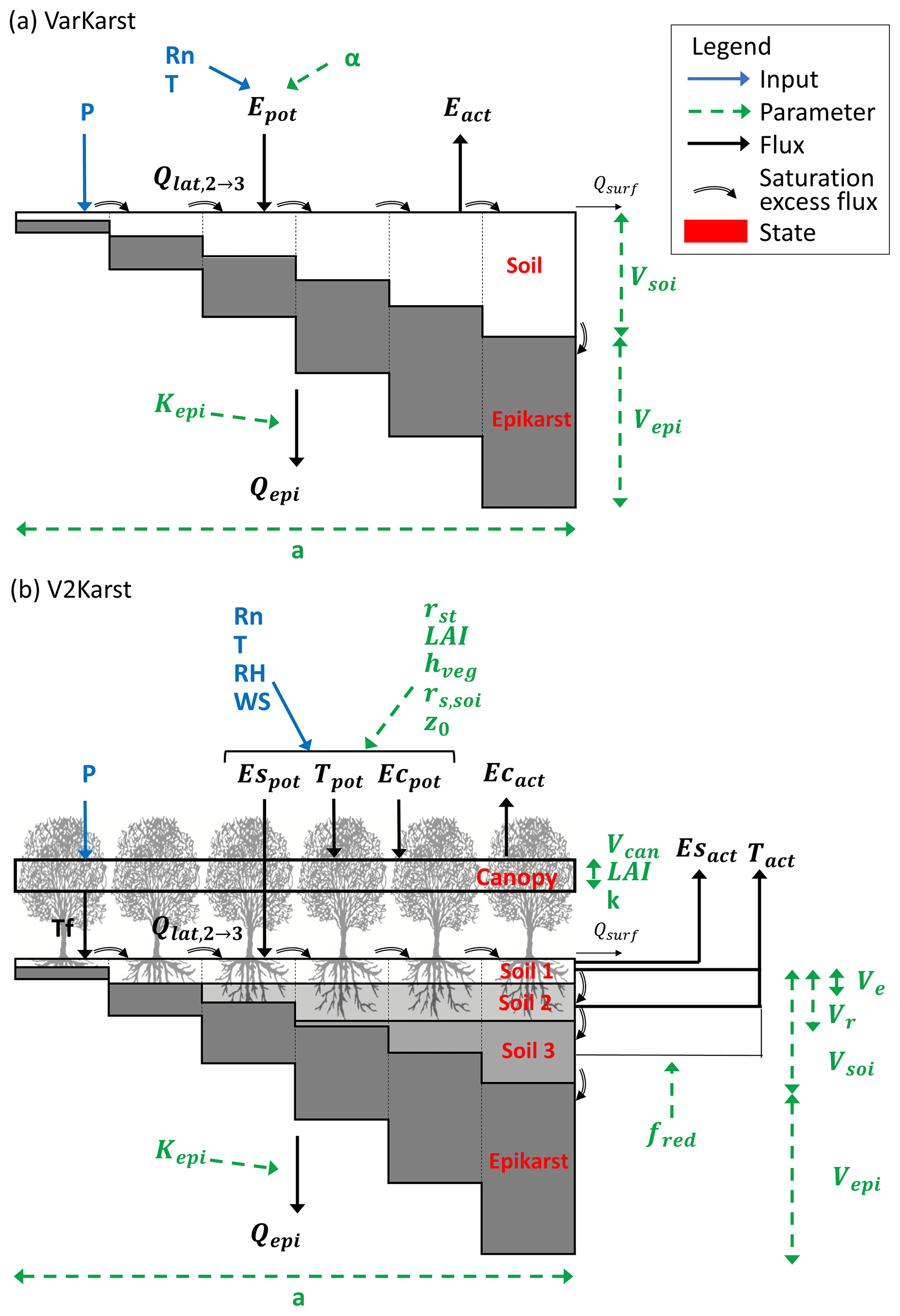
Figure 1 Schematic representation of (a) the VarKarst model (Hartmann et al., 2015) and (b) the new version of the model V2Karst using six vertical compartments. Model parameters are in green (see their definition in Table 1), inputs are in blue (P – precipitation, R_n – net radiation, T – temperature, RH – relative humidity, WS – wind speed), model fluxes are in black (E_pot – potential total evapotranspiration, T_pot – potential transpiration, Ec_pot – potential evaporation from canopy interception, Es_pot – potential soil evaporation, E_act – total actual ET, T_act – actual transpiration, Ec_act – actual evaporation from canopy interception, Es_act – actual bare soil evaporation, T_f – throughfall, $Q_{\text{lat},\mathrm{2}\to \mathrm{3}}$ – lateral flow from the second to the third compartment, Q_surf – surface runoff and Q_epi – recharge) and state variables are in red.

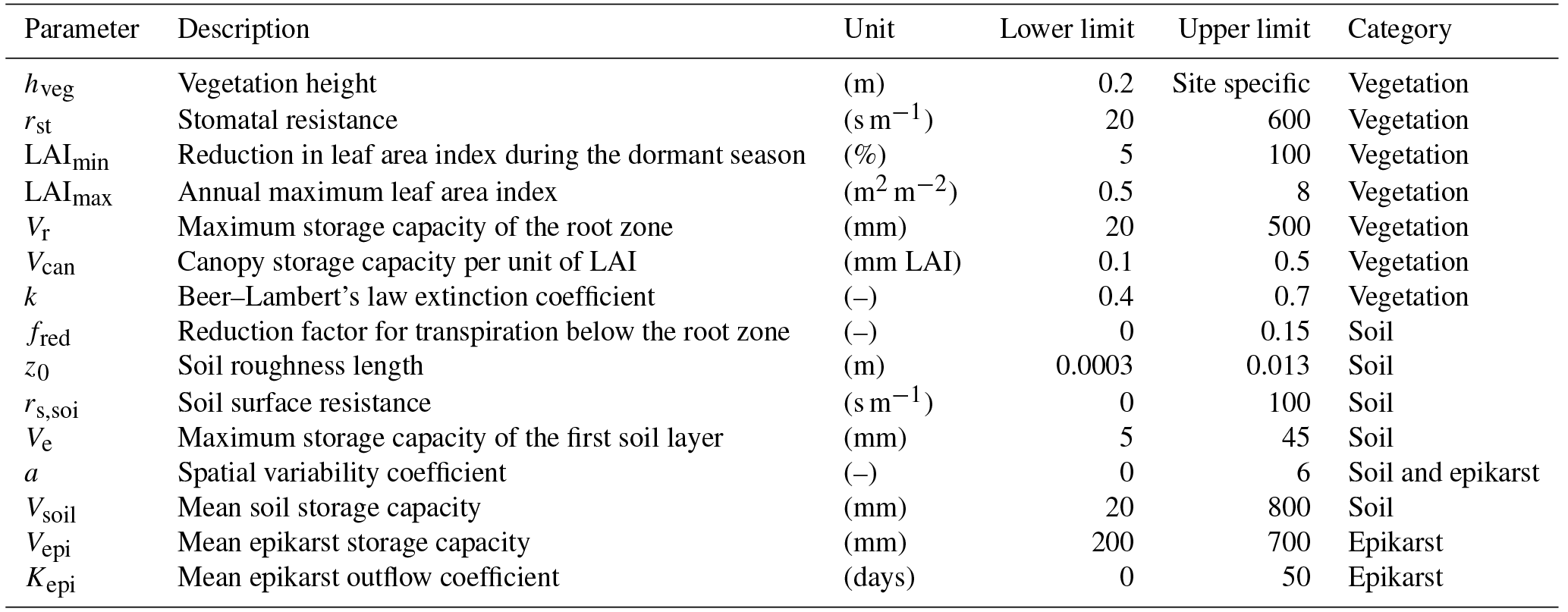
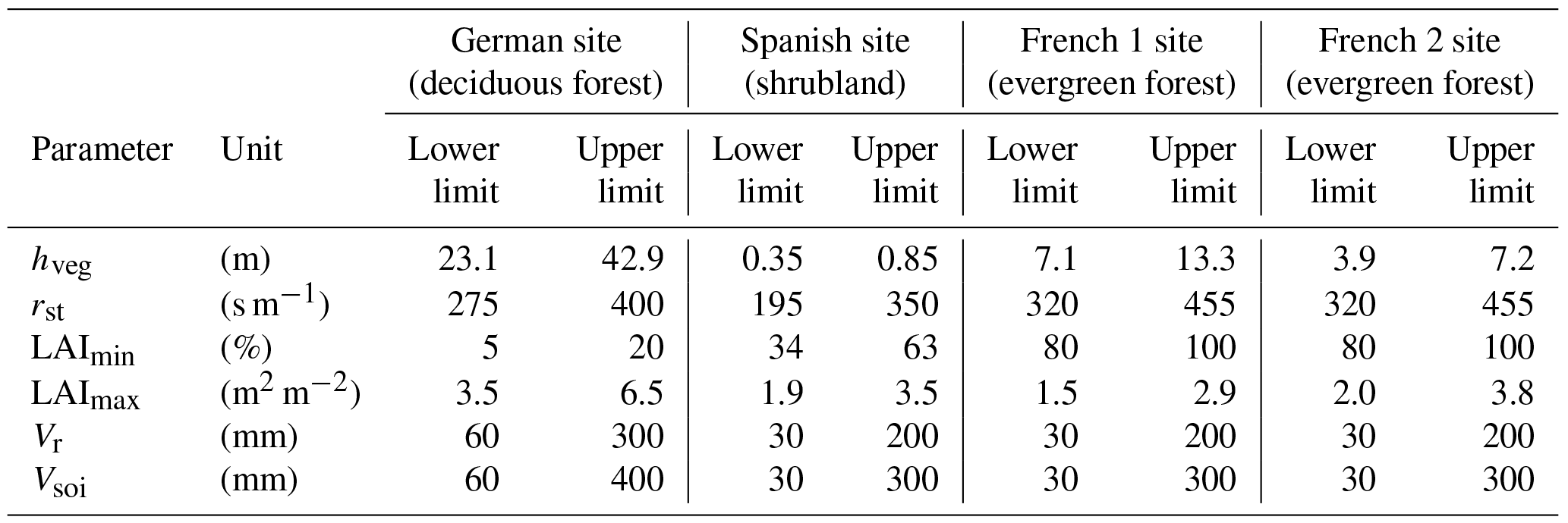
Table 1 Description of V2Karst parameters, unconstrained ranges used in the application at the four FLUXNET sites to capture the variability across soil, epikarst and vegetation types, and the category of the parameters (which indicates whether the parameters depend on soil, epikarst or vegetation properties). Parameters a, V_soil, V_epi and K_epi were already present in the previous version of the model (VarKarst). More information on how the ranges were determined is provided in Sect. S3 of our Supplement.

2.2 Previous representation of evapotranspiration (ET) processes in VarKarst

VarKarst (Hartmann et al., 2015) is currently the only karst recharge model developed for large-scale applications. It is a conceptual semi-distributed model that simulates karst potential recharge (Fig. 1a). The representation of karst processes in VarKarst is based on a previous karst model developed for applications at the local scale introduced in Hartmann et al. (2012b). VarKarst includes two horizontal subsurface layers, a top layer called “soil” and a deeper layer called “epikarst”. The soil layer corresponds to the layer from which ET can occur. The epikarst layer corresponds to the uppermost layer of weathered carbonate rocks where it is assumed that water cannot be lost through ET. VarKarst represents karst processes because for each model grid cell, the water balance is evaluated separately over a number of vertical compartments with varying soil and epikarst properties. Recharge is the flux leaving the bottom of the epikarst and is produced in saturated or unsaturated compartments where there is moisture stored in the epikarst. Recharge can occur at faster rates in deeper compared to shallower compartments. Additionally, lateral flow concentrates the infiltrating water from saturated to unsaturated compartments. Conceptually, the direct contribution of precipitation to infiltration and recharge can be associated with the diffuse fraction, while the contribution of lateral flow can be associated with the concentrated fraction. The model has been shown to be more appropriate for applications over karst areas than other large-scale hydrological models that do not represent karst processes (Hartmann et al., 2017). The ET component of the VarKarst model is very simple and does not include explicit representation of land cover properties. ET is lumped in the soil layer, is estimated from PET and is reduced by a water stress factor, which is estimated as a linear function of soil moisture. The PET rate is calculated with the empirical Priestley–Taylor equation (Priestley and Taylor, 1972) using a spatially and temporally uniform value of the empirical coefficient. This approach does not allow for the separation of the effects of climate and land cover, as the empirical coefficient reflects both climate and vegetation characteristics simultaneously. Therefore, the ET component of VarKarst needs to be modified if the model is to be used for large-scale land cover change impact assessment.

2.3 V2Karst: the new version of VarKarst for integrated vegetation–recharge simulations over karst areas

In this section, we propose a new version of the VarKarst model, called V2Karst (Sarrazin et al., 2018; Fig. 1b). In accordance with criteria 1 and 2 defined in Sect. 2.1, the new V2Karst model includes a physically based PET equation, separates the evapotranspiration flux into three components (transpiration, bare soil evaporation and evaporation from canopy interception) and comprises three soil layers. In agreement with criteria 3 of Sect. 2.1 (parsimony), we sought to parsimoniously represent the different ET processes in VarKarst. In fact, V2Karst uses 12 parameters to represent ET and vegetation seasonality, namely 11 newly introduced parameters that replace the Priestley–Taylor empirical coefficient α used in Varkarst and the soil water capacity parameter V_soi already present in VarKarst (model parameters are described in Table 1 and Fig. 1). This is less than other existing large-scale models that use the Penman–Monteith equation and separate the three ET components, as these models have over 15 parameters in their ET component (PCR-GLOBWB, VIC and the model of Kergoat, 1998, shown in Tables A1–A3). We assumed homogeneous above ground vegetation properties across model compartments.

The new model is forced by time series of precipitation (P), air temperature (T) and net radiation (R_n) in the same manner as VarKarst. Additionally, time series of relative humidity (RH) and wind speed (WS) are now needed for PET calculation. The V2Karst model can be run at both daily and sub-daily time steps. In this study, we present simulation results obtained using a daily time step, while results from hourly simulations are reported in Sect. S8 of our Supplement. We did not find significant differences between daily and hourly simulations for assessing recharge at monthly and annual timescales, which is the focus of our study. Therefore, it is reasonable to apply the model at a daily time step, which significantly reduces the computational requirements.

2.3.1 Definition of soil and epikarst properties in V2Karst

The computation of the water storage capacity of the entire soil column V_S,i (mm) and of the epikarst V_E,i (mm), and the epikarst outflow coefficient K_E,i (days) for the ith model compartment is carried out in the same fashion as in VarKarst:

$$\begin{array}{ll}{\displaystyle }& {\displaystyle }{V}_{\text{S},i}=V_{\text{max,S}}{\left({\displaystyle \frac{i}{n_{\text{c}}}}\right)}^a\\ \text{(1)}& {\displaystyle }& {\displaystyle }{V}_{\text{E},i}=V_{\text{max,E}}{\left({\displaystyle \frac{i}{n_{\text{c}}}}\right)}^a{\displaystyle }& {\displaystyle }{K}_{\text{E},i}=K_{\text{max,E}}{\left({\displaystyle \frac{n_{\text{c}}-i+\mathrm{1}}{n_{\text{c}}}}\right)}^a,\end{array}$$

where V_max,S (mm) is the maximum soil storage capacity over all model compartments; V_max,E (mm) is the maximum epikarst storage capacity; K_max,E (days) is the maximum outflow coefficient; n_c (–) is the number of model compartments, which is set to 15 following (Hartmann et al., 2013, 2015); and a (–) is the spatial variability coefficient. A previous study showed that V_S,i, V_E,i and K_E,i can be determined using the same distribution coefficient a (Hartmann et al., 2013). In V2Karst, V_max,S, V_max,E and K_E,i are computed as a function of the average properties of the cell using the following formulas:

$$\begin{array}{ll}{\displaystyle }& {\displaystyle }{V}_{\text{max,S}}={\displaystyle \frac{V_{\text{soi}}{n}_{\text{c}}}{\sum _{i=\mathrm{1}}^n{\left(\frac{i}{n_{\text{c}}}\right)}^a}}\\ \text{(2)}& {\displaystyle }& {\displaystyle }{V}_{\text{max,E}}={\displaystyle \frac{V_{\text{epi}}{n}_{\text{c}}}{\sum _{i=\mathrm{1}}^n{\left(\frac{i}{n_{\text{c}}}\right)}^a}}{\displaystyle }& {\displaystyle }{K}_{\text{max,E}}={\displaystyle \frac{K_{\text{epi}}{n}_{\text{c}}}{\sum _{i=\mathrm{1}}^n{\left(\frac{i}{n_{\text{c}}}\right)}^a}},\end{array}$$

where V_soi (mm) is the mean soil storage capacity, V_epi (mm) is the mean epikarst storage capacity and K_epi (mm) is the mean epikarst outflow coefficient. We note that the definition of the three parameters V_soi, V_epi and K_epi is revised compared to VarKarst.

As in VarKarst, we neglect ET from the epikarst. Several studies have shown that in the presence of shallow soil and a dry climate, plants can take up water in the weathered bedrock where soil pockets can sustain root development (Schwinning, 2010). However, given the uncertainty in soil depth for large-scale applications, V2Kast does not allow ET from the epikarst to avoid over-parameterisation. Therefore, the V2Karst soil layer must be interpreted as a conceptual layer that does not exactly correspond to the physical soil layer (layer of loose material) but is defined as the portion of the subsurface where ET losses can occur.

In V2Karst, the soil layer is further divided into a shallow top layer from which water can be lost from both evaporation and transpiration, a second middle layer where only transpiration can occur and a third deeper layer below the root zone where transpiration can only take place when the first two layers are depleted. The maximum storage capacity of the first layer is noted as V_e (mm), and the maximum storage capacity of first and second layers combined is noted as V_r (mm), which corresponds to the maximum storage capacity of the root zone. The model assumes that V_e is smaller than V_r, which is in turn smaller than the storage capacity of the deeper model compartment V_S,n.

2.3.2 Soil water balance

The soil water storage $V_{\text{soi},i}^j\left(t\right)$ (mm) in the ith compartment and the jth soil layer $j=\mathrm{1},\mathrm{2},\mathrm{3}$ is updated at the end of each time step t as follows:

$$\begin{array}{ll}{\displaystyle }{V}_{\text{soi},i}^{\mathrm{1}}\left(t\right)=& {\displaystyle }{V}_{\text{soi},i}^{\mathrm{1}}(t-\mathrm{1})+T_{\text{f}}\left(t\right)+Q_{\text{lat},i-\mathrm{1}\to i}\left(t\right)\\ {\displaystyle }& {\displaystyle }-{\text{Es}}_{\text{act},i}\left(t\right)-T_{\text{act},i}^{\mathrm{1}}\left(t\right)-R_{\mathrm{12},i}\left(t\right)\\ \text{(3)}& {\displaystyle }{V}_{\text{soi},i}^{\mathrm{2}}\left(t\right)=& {\displaystyle }{V}_{\text{soi},i}^{\mathrm{2}}(t-\mathrm{1})+R_{\mathrm{12},i}\left(t\right)-T_{\text{act},i}^{\mathrm{2}}\left(t\right)-R_{\mathrm{23},i}\left(t\right){\displaystyle }{V}_{\text{soi},i}^{\mathrm{3}}\left(t\right)=& {\displaystyle }{V}_{\text{soi},i}^{\mathrm{3}}(t-\mathrm{1})+R_{\mathrm{23},i}\left(t\right)-T_{\text{act},i}^{\mathrm{3}}\left(t\right)-R_{\text{epi},i}\left(t\right),\end{array}$$

where T_f(t) (mm) is the throughfall i.e. the fraction of precipitation that reaches the ground (Eq. 8), $Q_{\text{lat},i-\mathrm{1}\to i}\left(t\right)$ (mm) is the lateral flow from the (i−1)th to the ith model compartment (Sect. 2.3.4), Es_act,i(t) (mm) is the actual soil evaporation (Eq. 9), $T_{\text{act},i}^j\left(t\right)$(mm) is the actual transpiration in the jth soil layer (Eqs. 11–12), R_12,i(t) (mm) is the downward flow from the first to the second soil layer, R_23,i(t) (mm) is the downward flow from the second to the third soil layer and R_epi,i(t) (mm) is the downward flow from the soil to the epikarst.

It is assumed that percolation from the unsaturated soil to the epikarst is negligible due to the low permeability of the soil. This assumption seems reasonable as karst soils usually have a high clay content (Blume et al., 2010; Clapp and Hornberger, 1978). However, clayey soil typically presents cracks (Lu et al., 2016); therefore, when the soil reaches saturation, preferential flow starts to occur in the soil cracks, which causes all saturation excess to quickly infiltrate to the epikarst. Just as in VarKarst, such preferential vertical flow is represented by the variable R_epi,i(t) (used in Eq. 3) and is set equal to the saturation excess in the (lowest) soil layer. In V2Karst, a similar approach is also used to assess the other vertical flows from one soil layer to another (R_12,i(t) and R_23,i(t) in Eq. 3).

2.3.3 Evapotranspiration

We adopt the representation of sparse vegetation proposed by Bohn and Vivoni (2016) for the VIC model which is referred to as a “clumped” vegetation scheme. Each model compartment is divided into a vegetated and a non-vegetated fraction using a canopy cover fraction coefficient f_c(t) (–). The uptake of soil moisture for transpiration and soil evaporation is coupled in a way that, for each model compartment, we evaluate an overall water balance over the two fractions. Using a coupled approach such as this facilitates the representation of the seasonal variations in vegetated and non-vegetated fractions compared to an uncoupled “tile” approach, in which a separate soil moisture state is represented for vegetated and bare soil fractions. Consistent with other existing large-scale models, aerodynamic interactions between both fractions are neglected to keep the number of parameters to a minimum (Table A3).

The canopy coefficient f_c(t) is estimated in V2Karst using the Beer–Lambert's law as in Van Dijk and Bruijnzeel (2001) and Ruiz et al. (2010). This law was originally used to separate the fraction of incident radiation (and by extension of net radiation) absorbed by the canopy from the fraction penetrating the canopy (Kergoat, 1998; Ross, 1975; Shuttleworth and Wallace, 1985). The canopy cover fraction at time t is expressed as a function of the cell average leaf area index LAI(t) (m² m⁻²) and an extinction coefficient k (–), which is understood to vary across vegetation types as it accounts for leaf architecture (Ross, 1975):

$$\begin{array}{}\text{(4)}& {\displaystyle }{f}_{\text{c}}\left(t\right)=\mathrm{1}-e^{-k\text{LAI}\left(t\right)}.\end{array}$$

Notice that Eq. (4) allows for the description of the seasonal variations in the canopy cover fraction without introducing additional parameters in the model, given that it will simply follow the seasonal variations in the LAI.

Canopy interception

The interception storage capacity over the vegetated fraction V_can,max(t) (mm) depends (1) on the leaf area index over the vegetated fraction, which is estimated by rescaling the cell average leaf area index LAI(t) by the vegetation cover fraction f_c(t) (as in Bohn and Vivoni, 2016) and (2) on the canopy storage capacity per unit of leaf area index, denoted by V_can, which is understood to depend on the vegetation type since it accounts for leaf architecture (Gerrits, 2010). Specifically, it is expressed as

$$\begin{array}{}\text{(5)}& {\displaystyle }{V}_{\text{can,max}}\left(t\right)=V_{\text{can}}\left({\displaystyle \frac{\mathrm{LAI}\left(t\right)}{f_{\text{c}}\left(t\right)}}\right).\end{array}$$

The interception storage over the vegetated fraction I_c(t) (mm) is then updated at each time step as follows:

$$\begin{array}{}\text{(6)}& {\displaystyle }{I}_{\text{c}}\left(t\right)=min\left(P\left(t\right)+I_{\text{c}}(t-\mathrm{1})-{\displaystyle \frac{E{c}_{\text{act}}\left(t\right)}{f_{\text{c}}\left(t\right)}},V_{\text{can,max}}\left(t\right)\right).\end{array}$$

The actual evapotranspiration from canopy interception Ec_act(t) (mm) is computed as

$$\begin{array}{}\text{(7)}& {\displaystyle }{\text{Ec}}_{\text{act}}\left(t\right)=f_{\text{c}}\left(t\right)min\left({\text{Ec}}_{\text{pot}}\left(t\right),P\left(t\right)+I_{\text{c}}(t-\mathrm{1}),V_{\text{can,max}}\left(t\right)\right),\end{array}$$

where Ec_pot(t) (mm) is the potential evaporation from canopy interception (Eq. 14) and P(t) (mm) is the precipitation. The factor f_c(t) in Eq. (7) accounts for the fact that evaporation from canopy occurs over the vegetated fraction only. Finally, the throughfall is calculated as

$$\begin{array}{}\text{(8)}& {\displaystyle }{T}_{\text{f}}\left(t\right)=max\left(P\left(t\right)-{\text{Ec}}_{\text{act}}\left(t\right)-f_{\text{c}}\left(t\right)\left(I_{\text{c}}\left(t\right)-I_{\text{c}}(t-\mathrm{1})\right),\mathrm{0}\right).\end{array}$$

Previous studies suggest that daily simulations of interceptions can provide reasonable results (Gerrits, 2010; De Groen, 2002; Savenije, 1997). For daily simulations, the model does not account for the carry-over of the interception storage from one day to the next, which means that I_c(t) is set to zero at the end of each day and that all precipitation which is not evaporated from the interception store becomes throughfall as in Gerrits (2010), De Groen (2002) and Savenije (1997). This assumption can be justified by the fact that the interception process is highly dynamic at a sub-daily timescale, because the canopy can go through several wetting–drying cycles within a day (Gerrits, 2010). Therefore, at a daily time step, the canopy layer must be interpreted as a conceptual layer, where the storage capacity does not exactly correspond to the physical storage capacity of the canopy (i.e. the amount of water that can be held at a given time) but to the cumulative amount of water that can be held by the canopy over one day (Gerrits, 2010).

Bare soil evaporation

It is assumed that soil evaporation is a faster process than transpiration, which is consistent with general knowledge on ET processes (Wang and Dickinson, 2012). Therefore, soil moisture can be first evaporated and then transpired if some available moisture remains for plant water uptake. Soil evaporation is withdrawn for the first soil layer as a function of the potential rate and soil moisture, similar to the previous version of VarKarst:

$$\begin{array}{ll}\text{(9)}& {\displaystyle }& {\displaystyle }{\text{Es}}_{\text{act},i}\left(t\right)={\displaystyle }& {\displaystyle }min\left(\left(\mathrm{1}-f_{\text{c}}\left(t\right)\right){\text{Es}}_{\text{pot}}\left(t\right){\displaystyle \frac{V_{\text{soi},i}^{\mathrm{1}}(t-\mathrm{1})}{V_{\text{S},i}^{\mathrm{1}}}},V_{\text{soi},i}^{\mathrm{1}}(t-\mathrm{1})+T_{\text{f}}\left(t\right)\right),\end{array}$$

where Es_pot(t) is the potential soil evaporation (Eq. 14). The factor (1−f_c(t)) in Eq. (9) accounts for the fact that soil evaporation occurs from the non-vegetated fraction only; therefore, the potential rate has to be weighted by the bare soil cover fraction. The right term of the equation ($V_{\text{soi},i}^{\mathrm{1}}(t-\mathrm{1})+T_{\text{f}}\left(t\right))$ is not weighted because we assume that the soil moisture is uniform over the fractions of each model compartment (we compute a unique water balance); this means that the total moisture present in the first soil layer is available to soil evaporation because the vegetated fraction can supply moisture to the bare soil fraction.

Transpiration over the vegetated fraction

Transpiration mainly occurs in the first and second soil layers, and it switches to the third soil layer when the first two layers are depleted. The extraction of water by the roots below the root zone has been documented in studies such as Penman (1950). We account for this process by representing a soil layer below the root zone, which can provide water to the root zone through capillary rise as in the ISBA model (Boone et al., 1999). In V2Karst, the rate at which transpiration occurs in the two first soil layers $T_{\text{rate},i}^{\mathrm{12}}\left(t\right)$ (mm) and in the third soil layer $T_{\text{rate},i}^{\mathrm{3}}\left(t\right)$ (mm) are assessed as follows:

$$\begin{array}{ll}{\displaystyle }& {\displaystyle }{T}_{\text{rate},i}^{\mathrm{12}}\left(t\right)=\\ {\displaystyle }& {\displaystyle }\left(\mathrm{1}-t_{\text{wet}}\left(t\right)\right)f_{\text{c}}\left(t\right)T_{\text{pot}}\left(t\right){\displaystyle \frac{V_{\text{soi},i}^{\mathrm{1}}(t-\mathrm{1})+V_{\text{soi},i}^{\mathrm{2}}(t-\mathrm{1})}{V_{\text{S},i}^{\mathrm{1}}+V_{\text{S},i}^{\mathrm{2}}}}\\ \text{(10)}& {\displaystyle }& {\displaystyle }{T}_{\text{rate},i}^{\mathrm{3}}\left(t\right)={\displaystyle }& {\displaystyle }\left(\mathrm{1}-t_{\text{wet}}\left(t\right)\right)f_{\text{c}}\left(t\right)T_{\text{pot}}\left(t\right){\displaystyle \frac{V_{\text{soi},i}^{\mathrm{3}}(t-\mathrm{1})}{V_{\text{S},i}^{\mathrm{3}}}}{f}_{\text{red}},\end{array}$$

where T_pot(t) is the potential transpiration (Eq. 14), t_wet(t) (–) is the fraction of the time step with a wet canopy (Eq. 13) and f_red (–) is a reduction factor which accounts for the fact that moisture below the root zone is less easily accessible to the roots than moisture in the root zone (Penman, 1950); f_red is expected to vary across soil type since it is linked to the soil capability to supply water to the root zone. It is assumed that transpiration occurs in the two first soil layers when $T_{\text{rate},i}^{\mathrm{12}}\left(t\right)$ is higher than $T_{\text{rate},i}^{\mathrm{3}}\left(t\right)$, and that transpiration is drawn from the third soil layer otherwise. The actual transpiration in the two first soil layers $T_{\text{act},i}^{\mathrm{12}}\left(t\right)$ (mm) and in the third soil layer $T_{\text{act},i}^{\mathrm{3}}\left(t\right)$ (mm) are therefore calculated as follows:

$$\begin{array}{ll}{\displaystyle }& {\displaystyle }\text{when}{T}_{\text{rate},i}^{\mathrm{12}}\left(t\right)\ge T_{\text{rate},i}^{\mathrm{3}}\left(t\right):\\ \text{(11)}& {\displaystyle }& {\displaystyle }\left\{\begin{array}{l}{T}_{\text{act},i}^{\mathrm{12}}\left(t\right)=min\left(T_{\text{rate},i}^{\mathrm{12}}\left(t\right),V_{\text{soi},i}^{\mathrm{1}}(t-\mathrm{1})+V_{\text{soi},i}^{\mathrm{2}}(t-\mathrm{1})\right.\\ +T_{\text{f}}\left(t\right)-{\text{Es}}_{\text{act},i}\left(t\right)),\\ T_{\text{act},i}^{\mathrm{3}}\left(t\right)=\mathrm{0},\end{array}\right.{\displaystyle }& {\displaystyle }\text{when}{T}_{\text{rate},i}^{\mathrm{12}}\left(t\right)<T_{\text{rate},i}^{\mathrm{3}}\left(t\right):\\ {\displaystyle }& {\displaystyle }\left\{\begin{array}{l}{T}_{\text{act},i}^{\mathrm{12}}\left(t\right)=\mathrm{0},\\ T_{\text{act},i}^{\mathrm{3}}\left(t\right)=min\left(T_{\text{rate},i}^{\mathrm{3}}\left(t\right),V_{\text{soi},i}^{\mathrm{3}}(t-\mathrm{1})+R_{\mathrm{23},i}\left(t\right)\right)\end{array}\right..\end{array}$$

Actual transpiration in the upper two layers $T_{\text{act},i}^{\mathrm{12}}\left(t\right)$ is partitioned between the two soil layers within the root zone as is used in the PCR-GLOBWB model (Van Beek, 2008). In V2Karst, the transpiration is attributed to the two first soil layers proportional to their storage content. This simple representation assumes that the roots can equally access the moisture stored in the first and second layer. Actual transpiration from the first layer $T_{\text{act},i}^{\mathrm{1}}\left(t\right)$ (mm) and the second layer $T_{\text{act},i}^{\mathrm{2}}\left(t\right)$ (mm) are computed as follows:

$$\begin{array}{ll}{\displaystyle }& {\displaystyle }{T}_{\text{act},i}^{\mathrm{1}}\left(t\right)=\\ {\displaystyle }& {\displaystyle \frac{V_{\text{soi},i}^{\mathrm{1}}(t-\mathrm{1})+T_{\text{f}}\left(t\right)-{\text{Es}}_{\text{act},i}\left(t\right)}{V_{\text{soi},i}^{\mathrm{1}}(t-\mathrm{1})+T_{\text{f}}\left(t\right)-{\text{Es}}_{\text{act},i}\left(t\right)+V_{\text{soi},i}^{\mathrm{2}}(t-\mathrm{1})}}{T}_{\text{act},i}^{\mathrm{12}}\left(t\right)\\ \text{(12)}& {\displaystyle }& {\displaystyle }{T}_{\text{act},i}^{\mathrm{2}}\left(t\right)={\displaystyle }& {\displaystyle \frac{V_{\text{soi},i}^{\mathrm{2}}(t-\mathrm{1})}{V_{\text{soi},i}^{\mathrm{1}}(t-\mathrm{1})+T_{\text{f}}\left(t\right)-{\text{Es}}_{\text{act},i}\left(t\right)+V_{\text{soi},i}^{\mathrm{2}}(t-\mathrm{1})}}{T}_{\text{act},i}^{\mathrm{12}}\left(t\right).\end{array}$$

The fraction of the day with a wet canopy t_wet(t) (–) is estimated as the fraction of available energy that was used to evaporate water from the interception store similar to Kergoat  (1998):

$$\begin{array}{}\text{(13)}& {\displaystyle }{\displaystyle }{t}_{\text{wet}}\left(t\right)={\displaystyle \frac{{\text{Ec}}_{\text{act}}\left(t\right)}{f_{\text{c}}\left(t\right){\text{Ec}}_{\text{pot}}\left(t\right)}}.\end{array}$$

Potential evapotranspiration

We replace the Priestley–Taylor potential evaporation equation originally used in VarKarst with the Penman–Monteith equation (Monteith, 1965), which has been shown to be applicable at both a daily and sub-daily time step (e.g. Allen et al., 2006; Pereira et al., 2015). The potential transpiration rate over the vegetated fraction of the cell T_pot(t) (mm) is estimated from the canopy aerodynamic resistance r_a,can(t) (s m⁻¹) and surface resistance r_s,can(t) (s m⁻¹), the potential evaporation from interception over the vegetated fraction of the cell Ec_pot(t) (mm) is assessed assuming that the surface resistance is equal to 0 following studies such as Shuttleworth (1993), and the potential bare soil evaporation rate over the bare soil fraction of the cell Es_pot(t) (mm) is calculated from the soil aerodynamic resistance r_a,soi(t) (s m⁻¹) and surface resistance r_s,soi (s m⁻¹), using the following equations:

$$\begin{array}{ll}{\displaystyle }& {\displaystyle }{T}_{\text{pot}}\left(t\right)={\displaystyle \frac{\mathrm{\Delta }\left(t\right)\left(R_{\text{n}}\right(t)-G(t\left)\right)+K_{\text{t}}{\mathit{\rho }}_{\text{a}}\left(t\right)c_{\text{p}}\frac{e_{\text{s}}\left(t\right)-e_{\text{a}}\left(t\right)}{r_{\text{a,can}}\left(t\right)}}{\mathit{\lambda }\left(t\right)\left(\mathrm{\Delta }\left(t\right)+\mathit{\gamma }\left(t\right)\left(\mathrm{1}+\frac{r_{\text{s,can}}\left(t\right)}{r_{\text{a,can}}\left(t\right)}\right)\right)}}\\ \text{(14)}& {\displaystyle }& {\displaystyle }{\text{Ec}}_{\text{pot}}\left(t\right)={\displaystyle \frac{\mathrm{\Delta }\left(t\right)\left(R_{\text{n}}\right(t)-G(t\left)\right)+K_t{\mathit{\rho }}_{\text{a}}\left(t\right)c_{\text{p}}\frac{e_{\text{s}}\left(t\right)-e_{\text{a}}\left(t\right)}{r_{\text{a,can}}\left(t\right)}}{\mathit{\lambda }\left(t\right)\left(\mathrm{\Delta }\left(t\right)+\mathit{\gamma }\left(t\right)\right)}}{\displaystyle }& {\displaystyle }{\text{Es}}_{\text{pot}}\left(t\right)={\displaystyle \frac{\mathrm{\Delta }\left(t\right)\left(R_{\text{n}}\right(t)-G(t\left)\right)+K_t{\mathit{\rho }}_{\text{a}}\left(t\right)c_{\text{p}}\frac{e_{\text{s}}\left(t\right)-e_{\text{a}}\left(t\right)}{r_{\text{a,soi}}\left(t\right)}}{\mathit{\lambda }\left(t\right)\left(\mathrm{\Delta }\left(t\right)+\mathit{\gamma }\left(t\right)\left(\mathrm{1}+\frac{r_{\text{s,soi}}}{r_{\text{a,soi}}\left(t\right)}\right)\right)}},\end{array}$$

where R_n(t) (MJ m⁻² Δt⁻¹) is the net radiation (Δt is the simulation time step), G(t) (MJ m⁻² Δt⁻¹) is the ground heat flux, λ(t) (MJ kg⁻¹) is the latent heat of the vaporisation of water, Δ(t) (kPa ^∘C⁻¹) is the gradient of the saturated vapour pressure–temperature function, γ(t) (kPa ^∘C⁻¹) is the psychrometric constant, ρ_a(t) (kg m⁻³) is the air density, c_p (MJ kg^−1 ∘C⁻¹) is the specific heat of the air and is equal to $\mathrm{1.013}\times {\mathrm{10}}^{-\mathrm{3}}$ MJ kg^−1 ∘C⁻¹, e_s(t) (kPa) is the saturation vapour pressure, e_a(t) (kPa) is the actual vapour pressure and K_t (s Δt⁻¹) is a time conversion factor which corresponds to the number of seconds per simulation time step (equal to 86 400 s d⁻¹ for daily simulations). In this study, we neglect ground heat flux for the daily time step, which seems to be a reasonable assumption (see e.g. Allen et al., 1998; Shuttleworth, 2012).

The aerodynamic resistances of the canopy (r_a,can(t)) and the soil (r_a,soi(t)), which depend on the properties of the land cover and the soil, respectively, are computed using the formulation of Allen et al. (1998). To assess r_a,can(t), roughness lengths and the zero displacement plane for the canopy are estimated from the vegetation height h_veg (m) (Allen et al., 1998). To calculate r_a,soi(t)), the zero plane displacement height is equal to zero (d=0) and the roughness length for momentum and for heat and water vapour transfer are assumed to be equal, as in Šimůnek et al. (2009) and denoted as z₀ (m).

Finally, the canopy surface resistance is computed by scaling the stomatal resistance r_st (s m⁻¹) to the canopy level using the leaf area index over the vegetated fraction (as in Eq. 5 to assess canopy interception capacity); therefore, a homogeneous response across all stomata in the canopy is assumed (Allen et al., 1998; Liang et al., 1994):

$$\begin{array}{}\text{(15)}& {\displaystyle }{r}_{\text{s,can}}\left(t\right)={\displaystyle \frac{r_{\text{st}}}{\left(\frac{\text{LAI}\left(t\right)}{f_{\text{c}}\left(t\right)}\right).}}\end{array}$$

In other large-scale models, r_s,can is also often expressed as a function of the LAI, which allows for the direct representation of its seasonality following the variations in the LAI.

Seasonality of vegetation

We represent the seasonality of vegetation by describing the seasonal variation of the cell average LAI. We use two parameters, the maximum LAI_max (m² m⁻²), which is the annual maximum value of the LAI during the growing season (assumed to be from June to August in this study) and LAI_min (%), which is the percentage reduction in the LAI during the dormant season (assumed to be from December to February in this study). The monthly value of the leaf area index LAI_m (m² m⁻²) for the mth month is computed using a continuous, piecewise linear function of LAI_max and LAI_min, which allows for a smooth transition between dormant and growing seasons and is similar to the function proposed by Allen et al. (1998) to assess the seasonality in crop factors:

$$\begin{array}{}\text{(16)}& {\displaystyle }\begin{array}{l}{\text{LAI}}_m={\displaystyle \frac{{\text{LAI}}_{\text{min}}}{\mathrm{100}}}{\text{LAI}}_{\text{max}}\\ \text{when}m=\mathrm{1},\mathrm{2},\mathrm{12}\\ {\text{LAI}}_m={\displaystyle \frac{{\text{LAI}}_{\text{min}}}{\mathrm{100}}}{\displaystyle \frac{{\text{LAI}}_{\text{max}}}{\mathrm{4}}}\left(\mathrm{6}-m\right)+{\displaystyle \frac{{\text{LAI}}_{\text{max}}}{\mathrm{4}}}(m-\mathrm{2})\\ \text{when}m=\mathrm{3},\mathrm{4},\mathrm{5}\\ {\text{LAI}}_m={\text{LAI}}_{\text{max}}\\ \text{when}m=\mathrm{6},\mathrm{7},\mathrm{8}\\ {\text{LAI}}_m={\displaystyle \frac{{\text{LAI}}_{\text{min}}}{\mathrm{100}}}{\displaystyle \frac{{\text{LAI}}_{\text{max}}}{\mathrm{4}}}(m-\mathrm{8})+{\displaystyle \frac{{\text{LAI}}_{\text{max}}}{\mathrm{4}}}(\mathrm{12}-m)\\ \text{when}m=\mathrm{9},\mathrm{10},\mathrm{11}.\end{array}\end{array}$$

The advantage of using this simple parameterisation is that it permits one to easily analyse the effect of vegetation seasonality by studying the sensitivity of the model predictions to the LAI_min parameter, which captures the strength of the seasonal variation in LAI. Timings of the four phases of the seasonality model reported in Eq. (16) are adapted for the application at the sites used in the present study, which are all located in Europe (Sect. 3.1).

2.3.4 Water storage in the epikarst

Epikarst water storage V_epi,i(t) (mm) for the ith compartment is updated at the end of each time step t as follows:

$$\begin{array}{ll}{\displaystyle }& {\displaystyle }{V}_{\text{epi},i}\left(t\right)=V_{\text{epi},i}(t-\mathrm{1})+R_{\text{epi},i}\left(t\right)\\ {\displaystyle }& {\displaystyle }-Q_{\text{epi},i}\left(t\right)-Q_{\text{lat},i\to i+\mathrm{1}}\left(t\right)\\ \text{(17)}& {\displaystyle }& {\displaystyle }\text{when}i<n_{\text{c}}{\displaystyle }& {\displaystyle }{V}_{\text{epi},n_{\text{c}}}\left(t\right)=V_{\text{epi},n_{\text{c}}}(t-\mathrm{1})+R_{\text{epi},n_{\text{c}}}\left(t\right)\\ {\displaystyle }& {\displaystyle }-Q_{\text{epi},n_{\text{c}}}\left(t\right)-Q_{\text{surf},n_{\text{c}}}\left(t\right)\\ {\displaystyle }& {\displaystyle }\text{when}i=n_{\text{c}},\end{array}$$

where Q_epi,i(t) (mm) is the potential recharge to the groundwater (Eq. 18), $Q_{\text{lat},i\to i+\mathrm{1}}\left(t\right)$ (mm) is the lateral flow from the ith to the (i+1)th model compartment and $Q_{\text{surf},n_{\text{c}}}\left(t\right)$ (mm) is the surface runoff generated by the n_cth compartment. When soil and epikarst layers are saturated, the concentration flow component of the model is activated. The ith model compartment generates lateral flow towards the (i+1)th compartment $Q_{\text{lat},i\to i+\mathrm{1}}\left(t\right)$ (mm) equal to its saturation excess. Lateral flow from the n_cth compartment is lost from the cell as surface runoff, while the other model compartments do not produce any surface runoff. The epikarst is simulated as a linear reservoir (Rimmer and Hartmann, 2012) with the outflow coefficient K_E,i (days):

$$\begin{array}{ll}\text{(18)}& {\displaystyle }& {\displaystyle }{Q}_{\text{epi},i}\left(t\right)={\displaystyle }& {\displaystyle }min\left({\displaystyle \frac{V_{\text{epi},i}(t-\mathrm{1})}{K_{\text{E},i}}},V_{\text{epi},i}(t-\mathrm{1})+R_{\text{epi},i}\left(t\right)\right).\end{array}$$

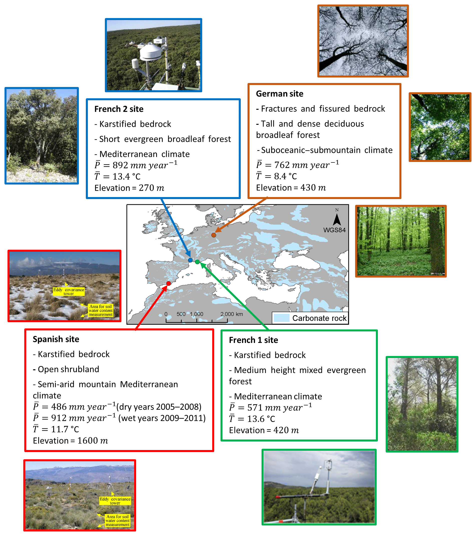
Figure 2 The four carbonate rock FLUXNET sites selected for the analyses. Mean annual precipitation ($\stackrel{\mathrm{‾}}{P}$) and mean annual temperature ($\stackrel{\mathrm{‾}}{T}$) were estimated over the period from 1 January 2001 to 17 December 2009 for the German site, 1 January 2006 to 31 December 2008 for the Spanish site (dry years), 1 January 2009 to 30 December 2011 for the Spanish site (wet years), 1 January 2010 to 30 December 2011 for the French 1 site and 1 April 2003 to 31 March 2009 for the French 2 site. Sources of the photos: Pinty et al. (2011) for the German site, Alcalá et al. (2011) for the Spanish site, http://www.gip-ecofor.org/f-ore-t/fontBlanche.php (last access: 30 November 2018) for the French 1 site, http://puechabon.cefe.cnrs.fr/ (last access: 30 November 2018) for the French 2 site. Source of the carbonate rock and country map: Williams and Ford (2006) (country map obtained from Terraspace, Russian space agency).

3 Sites and data for model testing

3.1 Description of study sites

We test the model with plot scale measurements from sites of the FLUXNET network (Baldocchi et al., 2001). We identified four FLUXNET sites across European and Mediterranean carbonate rock areas for which sufficient data were available to force V2Karst and to test the model (see Sect. 3.2). A short summary of each site's characteristics is provided in Fig. 2, and more detailed information can be found in Table B1.

The sites have different climate and land cover properties. The first site (Hainich site, referred to as “German site”) is located in the protected Hainich National Park, Thuringia, central Germany, and is characterised by a suboceanic–submountain climate and a tall and dense deciduous broadleaf forest. The second site (Llano de los Juanes site, referred to as “Spanish site”) is located on a plateau of the Sierra de Gádor mountains, south-eastern Spain, has a semi-arid mountain Mediterranean climate and is an open shrubland. The third site (Font-Blanche site, referred to as “French 1 site”) is located in south-eastern France, has a Mediterranean climate and its land cover is medium-height mixed evergreen forest. The fourth site (Puéchabon site, referred to as “French 2 site”) is located in southern France and is characterised by a Mediterranean climate with a short evergreen broadleaf forest. Overground vegetation properties are well characterised at all sites, but subsurface properties are more uncertain. In particular, the rooting depth water capacity was only well investigated at the French 2 site. The four sites are appropriate for testing V2Karst, as they satisfy the model assumptions: a karstified or fissured and fractured bedrock, overall high infiltration capacity with limited surface runoff and high clay content in the soil (Table B1).

3.2 Data description and preprocessing

Data available at the four FLUXNET sites include measurements of precipitation, temperature, net radiation, relative humidity and wind speed to force the model. Eddy-covariance measurements of latent heat flux (density) and at the German and Spanish sites measurements of soil moisture are also available to estimate the model parameters (Sect. 4.1). Specifically, at the German site, soil moisture was measured in one vertical soil profile at three different depths (5, 15 and 30 cm) with Theta probes (Knohl et al., 2003). We selected the measurement at 30 cm depth; we deemed this depth to be most representative of the entire soil column which has a depth between 50 and 60 cm. At the Spanish site, soil moisture was assessed at a depth of 15 cm using a water content reflectometer (Pérez-Priego et al., 2013).

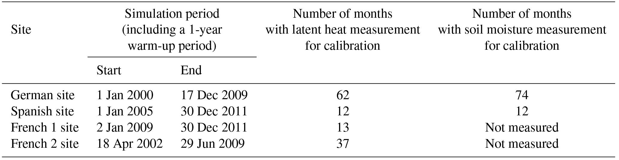
Table 2 Simulation period at the four FLUXNET sites, and number of months for which latent heat measurements and soil moisture measurements are available to calibrate the model. Soil moisture measurements are not provided at the two French sites.

Data to force the model were gap-filled and aggregated from a 30 min to a daily timescale. V2Karst output observations, namely latent heat flux and soil moisture measurements, were aggregated from a 30 min to a monthly timescale and we discarded the months when more than 20 % of the 30 min data were missing. We discarded the monthly observations of latent heat flux and soil moisture for months in which the forcing data contained many gaps; therefore, the impact of the gap-filling of the data on the simulation results is likely to be too significant to sensibly compare simulated and observed soil moisture and latent heat flux. Additionally, we removed monthly aggregated latent heat flux measurements when the mismatch in the energy balance closure was higher than 50 %, similar to Miralles et al. (2011). We corrected latent heat flux measurements to force the closure of the energy balance assuming that measured latent heat flux (LE; MJ m⁻² month⁻¹) and sensible heat flux (H; MJ m⁻² month⁻¹) have similar errors. The corrected evapotranspiration estimate (E_act,cor; mm month⁻¹) is calculated as proposed in Foken et al. (2012) and Twine et al. (2000):

$$\begin{array}{}\text{(19)}& {\displaystyle }{E}_{\text{act,cor}}={\displaystyle \frac{R_{\text{n}}}{\mathit{\lambda }\left(\mathrm{1}+\frac{H}{\text{LE}}\right)}}.\end{array}$$

Further details on the data processing and on the analysis of the uncertainty in latent heat flux measurements are reported in Sect. S4 of our Supplement. In particular, we showed that, while the actual value of the latent heat flux can have large uncertainties, we have a much higher confidence in its temporal variations.

Table 2 reports the simulation period and the number of monthly latent heat flux and soil moisture observations that were used to estimate the model parameters at the four FLUXNET sites. We extracted a continuous time series of forcing data covering about 10 years at the German site, 7 years at the Spanish site, 3 years at the French 1 site and 8 years at the French 2 site, while latent heat flux and soil moisture measurements were not available over the entire simulation time series. All model simulations were performed using a 1-year warm-up period, which we found to be sufficient to remove the impact of the initial conditions on the simulation results (see Sect. S5 of our Supplement).

4 Methods

To test the plausibility of V2Karst predictions at the FLUXNET sites, we run three sets of analyses: we first estimate the model parameters using actual ET and soil moisture observations available at the four sites (methods in Sect. 4.1); we then analyse the sensitivity of simulated annual recharge to the model parameters using measured forcing data to understand the controlling processes (Sect. 4.2); finally, we investigate the sensitivity of simulated recharge to precipitation properties and land cover type in virtual experiments, in order to understand the controlling processes in recharge when the forcing data is varied more widely than observed at the study sites (Sect. 4.3). All of the analyses were performed using the SAFE toolbox for global sensitivity analysis (Pianosi et al., 2015).

Table 3 Site-specific constrained parameter ranges at the four FLUXNET sites for the vegetation parameters (h_veg, r_st, LAI_min, LAI_max and V_r) and the soil storage capacity (V_soi). More information on how the ranges were determined is provided in Sect. S3 of our Supplement. Parameters are defined in Table 1.

4.1 Parameter constraints at the FLUXNET sites using soft rules

We investigate whether it is possible to estimate parameter values that produce plausible simulations based on information available at each FLUXNET site. To this end, and similarly to Hartmann et al. (2015), we use “soft rules” to accept or reject parameter combinations based on the consistency between monthly model simulations on one side, and monthly observations and a priori information on model fluxes on the other side. Using soft rules instead of “hard rules” (i.e. the minimisation of the mismatch between observations and simulations) allows for the identification of a set of plausible parameter sets and accounts for the fact that (1) the observed soil moisture is not strictly commensurate with simulated soil moisture, (2) observations are affected by uncertainties (see Sect. 3.2) and (3) it is not expected that V2Karst simulations closely match site-specific data, as the model structure is based on general understanding of karst systems for large-scale applications and may not account for some site specificities. We define five soft rules to identify acceptable (“behavioural”) parameter combinations:

1. The bias between observed and simulated actual ET is below 20 %:

   $$\begin{array}{}\text{(20)}& {\displaystyle }\text{Bias}=\left|{\displaystyle \frac{\sum _{t\in M_{\text{ET}}}\left(E_{\text{act,sim}}\right(t)-E_{\text{act,cor}}(t\left)\right)}{\sum _{t\in M_{\text{ET}}}{E}_{\text{act,cor}}\left(t\right)}}\right|<\mathrm{20}\mathit{\%},\end{array}$$

   where E_act,sim(t) (mm) is the simulated actual ET for month t (sum of transpiration, soil evaporation and evaporation from canopy interception), E_act,cor(t) (mm) is the corrected observed actual ET (Eq. 19) and M_ET is the set of months for which latent heat measurements are available. This rule allows one to constrain the simulated water balance.

2. The correlation coefficient (ρ_ET) between observed monthly actual ET (E_act,bw) and simulated total actual ET (E_act,sim) is above 0.6. This rule ensures that the temporal pattern of simulated ET follows the observed pattern.

3. The correlation coefficient (ρ_SM) between observed monthly soil moisture (SM_obs – % soil saturation) and simulated monthly soil moisture (SM_sim – m³ m⁻³ soil volume) is above 0.6. Simulated soil moisture SM_sim for month t is calculated as the average soil moisture within the root zone over all model compartments. This rule guarantees that soil moisture variations are consistent with observations.

4. Total simulated surface runoff (Q_surf) is less than 10 % of precipitation, in accordance with a priori information on the carbonate rock sites, which attests that runoff is negligible (see Sect. 3.1).

5. Soil and vegetation parameter values are consistent with a priori information, i.e. they fall within constrained (site-specific) ranges. This rule applies to the parameters for which a priori information is available at the FLUXNET sites, namely h_veg, r_st, LAI_min, LAI_max, V_r and V_soi and the constrained ranges are reported in Table 3. This rule ensures that acceptable model outputs are produced using plausible parameter values.

For each site, we derived a sample size of 100 000 for the 15 parameters of V2Karst using Latin hypercube sampling and unconstrained (wide) ranges for the model parameters to explore a large range of soil and vegetation types. We applied the above rules in sequence to either reject or accept the sampled parameter combinations. We sampled the constrained parameter ranges used in rule 5 more densely so that a sufficiently large number of parameterisations remain after applying rule 5. Similarly to Hartmann et al. (2015), a priori information on parameter ranges (rule 5) is applied last so that we can first assess the constraint of the parameter space based on information on model output only (rules 1–4); we then assess the consistency of the constraint using a priori information (rule 5).

We also note that the thresholds used in rules 1 to 3 are stricter than in the study by Hartmann et al. (2015), in which the threshold for the bias rule 1 was set to 75 % and for the correlation rules 2 and 3 was set to 0. The reason for this is that in Hartmann et al. (2015) behavioural parameter sets had to be consistent with observations at all sites within each climate zone defined in the study, while here we perform the parameter estimation for each site separately and therefore we expect better model performances.

4.2 Global sensitivity analysis

We use a global sensitivity analysis called the elementary effect test (Saltelli et al., 2008), also referred to as the method of Morris (1991), to analyse sensitivity across the entire space of parameter variability (Saltelli et al., 2008). We chose this method in particular because it is well suited for identifying uninfluential parameters (Campolongo et al., 2007; Saltelli et al., 2008), which is one of the objectives of our analysis, and because it can be applied to dependent parameters (in V2Karst it is assumed that $V_{\text{e}}\le V_{\text{r}}\le V_{\text{S},n}$ as explained in Sect. 2.3.1).

The method requires the computation of the elementary effects (EEs) of each parameter in n different baseline points in the parameter space. The EE of the ith parameter x_i at a given baseline point $\left(x_{\mathrm{1}}^j,x_{\mathrm{2}}^j,\mathrm{\dots },x_{i-\mathrm{1}}^j,x_i^j,\mathrm{\dots },x_M^j\right)$ and for a predefined perturbation Δ is assessed as follows:

$$\begin{array}{}\text{(21)}& {\displaystyle }{\text{EE}}_i^j={\displaystyle \frac{{\displaystyle \begin{array}{c}y\left(x_{\mathrm{1}}^j,x_{\mathrm{2}}^j,\mathrm{\dots },x_{i-\mathrm{1}}^j,x_i^j+\mathrm{\Delta },\mathrm{\dots }{x}_M^j\right)\\ -y\left(x_{\mathrm{1}}^j,x_{\mathrm{2}}^j,\mathrm{\dots },x_{i-\mathrm{1}}^j,x_i^j,\mathrm{\dots }{x}_M^j\right)\end{array}}}{\mathrm{\Delta }}},\end{array}$$

where M is the number of parameters and y is the model output (simulated annual recharge in our case). We analyse the mean of the absolute values of the EEs (denoted by ${\mathit{\mu }}_i^{*}$) introduced in Campolongo et al. (2007), which is a measure of the total effect of the ith parameter; we also analyse the standard deviation of the EEs (σ_i) proposed in Morris (1991), which is an aggregate measure of the intensity of the interactions of the ith parameter with the other parameters and of the degree of non-linearity in the model response to changes in the ith parameter.

The total number of model executions required to compute these two sensitivity indices is n(M+1), where n is the number of baseline points chosen by the user. The baseline points and the perturbation Δ of Eq. (21) were determined following the radial design proposed by Campolongo et al. (2011). The baseline points and the perturbation were randomly selected using Latin hypercube sampling for the 15 parameters of V2Karst, and dropping the parameter sets that did not meet the condition $V_{\text{e}}\le V_{\text{r}}\le V_{\text{S},n}$. In our application, we used n=500 points, which means that we needed 8000 model executions for each sensitivity analysis for each of the four FLUXNET sites. We derived confidence intervals on the sensitivity indices using 1000 bootstrap resamples, and checked the convergence of the results at the chosen sample size, as suggested in Sarrazin et al. (2016).

4.3 Virtual experiments to analyse sensitivity to climate and land cover change

Our last analysis consists of a set virtual experiments to investigate the sensitivity of recharge simulated by V2Karst to changes in (1) the precipitation properties, specifically monthly total precipitation and daily temporal distribution (i.e. frequency and intensity), which are likely to change (IPCC, 2013) and (2) land cover, specifically from forest to shrub or vice versa.

Virtual experiments permit full control of experimental conditions, thus, changes in model outputs can be unequivocally attributed to changes in model inputs (see e.g. Pechlivanidis et al., 2016; Weiler and McDonnell, 2004). Different studies have used virtual experiments to analyse the impact of precipitation spatial and temporal variability on hydrologic model outputs. In fact, using historical precipitation time series or future projections only allows for the exploration of a limited range of possible realisations, which makes it difficult to disentangle the effects of different precipitation properties on model outputs. Instead, synthetic precipitation time series can be tailored to analyse the impact of specific precipitation characteristics, for instance precipitation spatial distribution (Pechlivanidis et al., 2016; Van Werkhoven et al., 2008) and precipitation temporal distribution, namely frequency and intensity (Jothityangkoon and Sivapalan, 2009; Porporato et al., 2004), storminess (Jothityangkoon and Sivapalan, 2009), and seasonality (Botter et al., 2009; Jothityangkoon and Sivapalan, 2009; Laio et al., 2002; Yin et al., 2014).

In this study, we create a synthetic precipitation time series where the same precipitation event is periodically repeated. The precipitation time series is characterized by the intensity of precipitation events I_p (mm d⁻¹) and the interval between two wet days H_p (days). The duration of each precipitation event is set here to 1 day. Therefore, the average monthly precipitation P_m (mm month⁻¹) for an average month with 30 days is equal to:

$$\begin{array}{}\text{(22)}& {\displaystyle }{P}_{\text{m}}=\mathrm{30}{\displaystyle \frac{I_{\text{p}}}{\mathrm{1}+H_{\text{p}}}}.\end{array}$$

Table 4 Values of V2Karst parameters and weather variables used in the virtual experiments. Values for the virtual forest site and the virtual shrub site are based on the characteristics of the German FLUXNET site and Spanish FLUXNET site, respectively. Values of the model parameters (parameters are defined in Table 1) correspond to behavioural parameterisations obtained when calibrating the model at FLUXNET sites. Values of the weather variables (R_n – net radiation, T – temperature, RH – relative humidity and WS – wind speed) correspond to the average values calculated at FLUXNET sites.

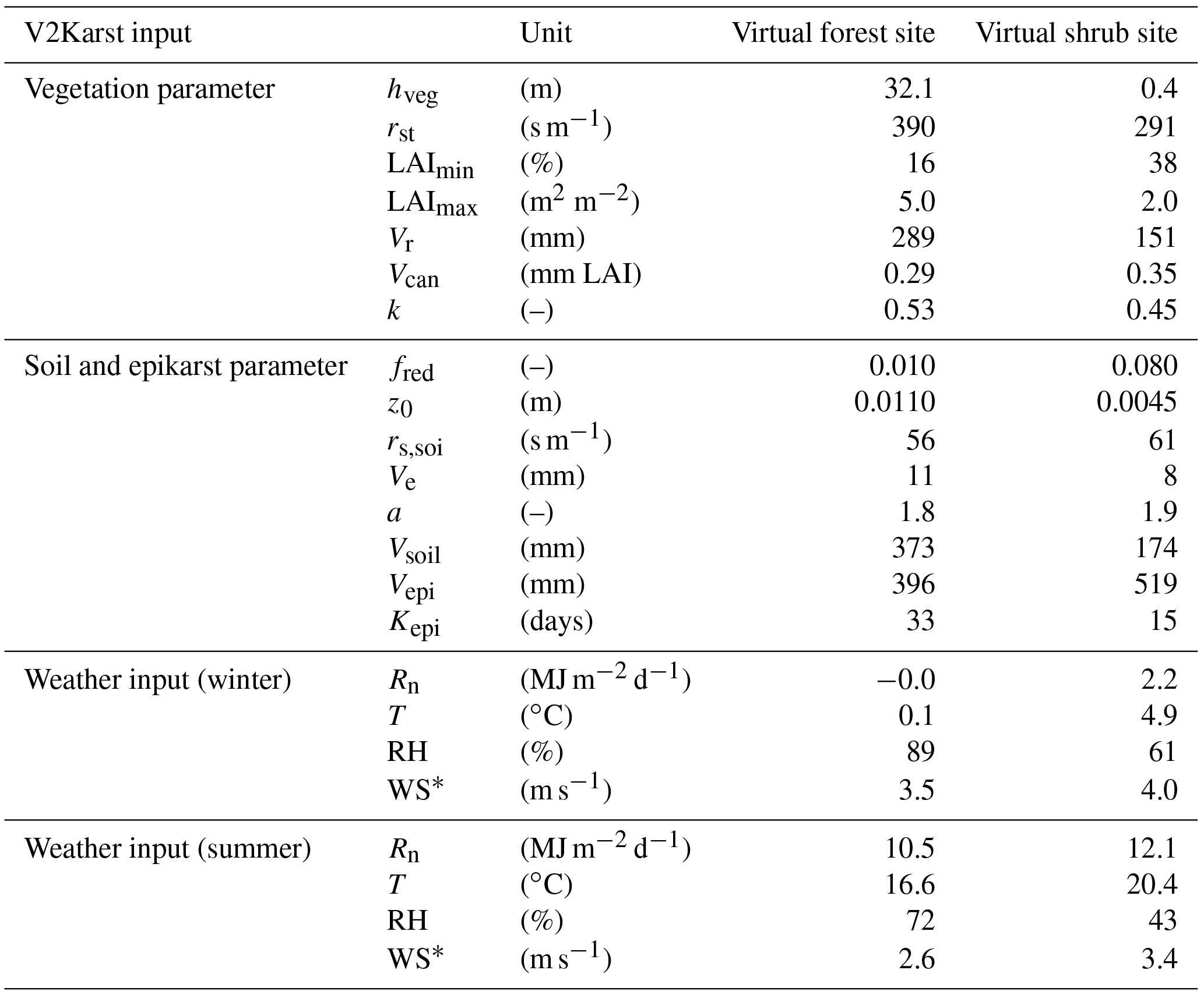
^* At the virtual shrub site, WS was recalculated at a height of 43.5 m because the original measurement provided at a height of 2.5 m at the Spanish site was too low to simulate a change of land cover to tall vegetation (forest). More details on this are reported in Sect. S4 of our Supplement.

To determine the possible range of variation of the three variables, P_m, I_p and H_p, we analysed their distributions at the four FLUXNET sites and over all European and Mediterranean carbonate rock areas using Global Land Data Assimilation System (GLAS) data (Rodell et al., 2004; distributions are reported in Sect. S6 of our Supplement). We found that wide but plausible ranges are as follows: P_m varies between 0 and 500 mm month⁻¹, I_p varies between 0 and 200 m d⁻¹ and H_p varies between 0 and 89 days (note that H_p=0 means that it rains every day). We then derived a set of 2266 precipitation time series by deterministically sampling P_m and H_p within those ranges (and consequently deriving a sampled value of I_p from Eq. 22). We sampled more densely closer to the lower bound of the ranges as this is where lower values of P_m and H_p are more likely to occur. For each of the precipitation time series obtained in this manner, we ran the V2Karst model until a steady-state was reached (i.e. periodic oscillations of all state and flux variables) and we analysed the steady-state monthly average of recharge.

The experiments are conducted at two “virtual sites” that are designed based on the characteristics of the FLUXNET sites. Specifically, we use a virtual “forest site” that has the characteristics of the German site (i.e. its behavioural parameterisations for the soil, epikarst and vegetation parameters, and its climate characteristics) as the baseline and a virtual “shrub site” that has the characteristics of the Spanish site. We do not investigate the effects of varying temperature, net radiation, relative humidity or wind speed characteristics as we did for precipitation, because these variables are correlated (see e.g. Ivanov et al., 2007) and, therefore, they cannot be varied independently. We account for their overall combined effect and we vary them jointly to reproduce two conditions, i.e. winter (low energy for ET) and summer (high energy for ET). For winter (summer) conditions we forced the model using constant values of temperature, net radiation, relative humidity and wind speed that were taken as the average values measured at the FLUXNET sites during winter (summer). To investigate the impact of a change in land cover, we swapped the vegetation parameters between the two virtual sites. Table 4 reports the values of the parameters and the values of the weather variables used at the two virtual sites.

Figure 3 Reduction in the number of behavioural parameterisations of the V2Karst model at the four FLUXNET sites, when sequentially applying the five soft rules defined in Sect. 4.1 (no rule – initial sample; rule 1 – ET bias; rule 2 – ET correlation; rule 3 – soil moisture correlation; rule 4 – runoff; and rule 5 – a priori information). Rule 3 could not be applied to the French sites where soil moisture observations were not available.

5 Results

5.1 Parameter constraints at FLUXNET sites

We first present the results of applying the soft rules defined in Sect. 4.1 at the four FLUXNET sites. Figure 3 shows that behavioural parameterisations consistent with all rules can be identified at all sites, although the number of parameterisations is very different from one site to another. Specifically, out of the initial 100 000 randomly generated parameter samples, we found 36 838 behavioural parameterisations at the German site, 147 at the Spanish site, 6354 at the French 1 site and 4077 at the French 2 site. From Fig. 3, we also see that the application of each rule reduces the number of behavioural parameterisations, except for rule 4 (value of total surface runoff <10 % of precipitation), as all model simulations produce less than 7 % surface runoff at all sites. This can be explained by the fact that V2Karst gives priority to recharge production over surface runoff. Therefore, the latter only occurs under extremely wet conditions when all model compartments are saturated.

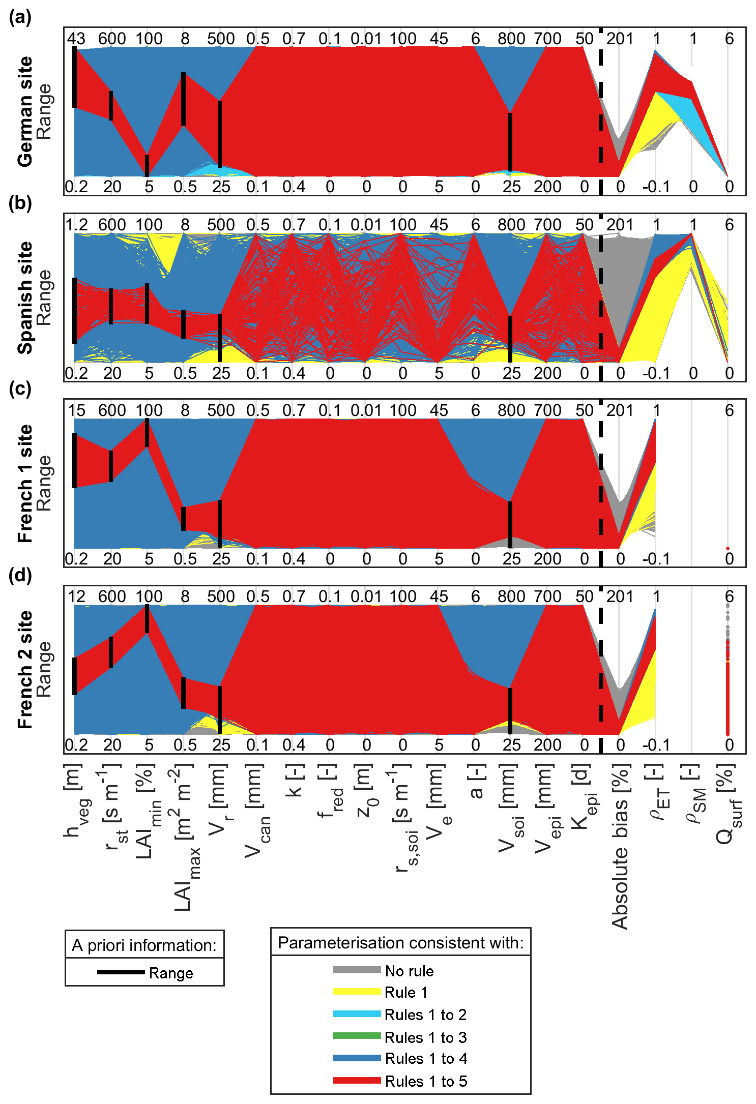
Figure 4 Parallel coordinate plots representing V2Karst behavioural parameterisations, and their corresponding simulated output values, identified when sequentially applying the five soft rules defined in Sect. 4.1 at (a) the German site, (b) the Spanish site, (c) the French 1 site and (d) the French 2 site. Parameters are defined in Table 1. The bias absolute mean error between observed and simulated total actual ET (rule 1), the ρ_ET correlation coefficient between observed and the simulated total actual ET (rule 2), the ρ_SM correlation coefficient between observed and simulated soil moisture (rule 3) and the Q_surf surface runoff (rule 4) are displayed on the right of the figure. Rule 5 corresponds to application of a priori information on parameter ranges (black vertical bars).

Figure 4 reports a parallel coordinate plot of the behavioural parameter sets and associated values of the output metrics after sequential application of the soft rules. The application of rules 1 to 4 does not significantly reduce the parameter ranges, but it allows for low values of parameters V_r and V_soi to be discarded at all sites (dark blue lines in Fig. 4). In contrast, the application of rule 5 (a priori parameter ranges, black vertical lines in Fig. 4) permits for a significant reduction in parameter ranges, not only for the parameters that are directly constrained by this rule (h_veg, r_st, LAI_min, LAI_max, V_r and V_soi) but also for the spatial variability coefficient a. Specifically, behavioural values of the a parameter are found to be between 0 and 3.2 at the French 1 site and between 0 and 2.8 at the French 2 site. At the Spanish site, we also observe that the behavioural simulations (red lines) cover some portions of the ranges more densely, specifically higher values of parameters r_s,soi and a, and lower values of z₀ and V_e. This means that the value for these parameters is more likely to be within these sub-ranges.

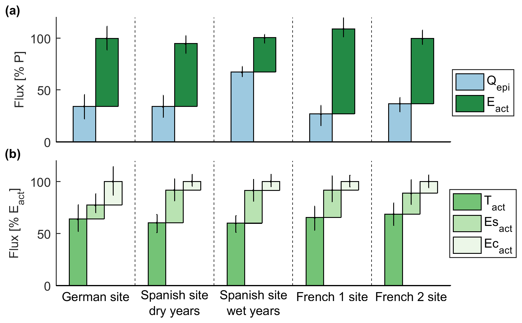
Figure 5 (a) Simulated recharge (Q_epi) and actual ET (E_act) expressed as a percentage of total precipitation, and (b) simulated actual transpiration (T_act), actual soil evaporation (Es_act) and actual evaporation from interception (Ec_act) expressed as a percentage of E_act. The figure reports the ensemble mean and 95 % confidence intervals calculated over the behavioural simulation ensemble of the V2Karst model at the four FLUXNET sites. Simulated fluxes were evaluated over the period from 1 January 2001 to 17 December 2009 for the German site, 1 January 2006 to 31 December 2008 for the Spanish site (dry years), 1 January 2009 to 30 December 2011 for the Spanish site (wet years), 1 January 2010 to 30 December 2011 for the French 1 site and 1 April 2003 to 31 March 2009 for the French 2 site.

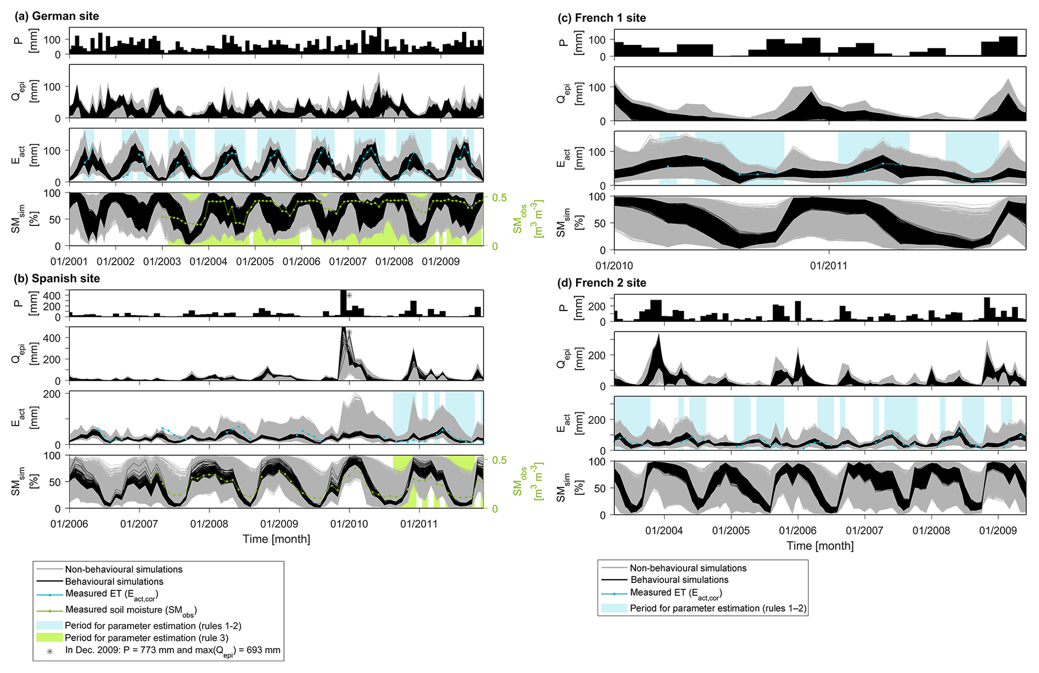
Figure 6 Monthly time series of observed variables, namely precipitation input P, actual ET E_act,cor (in blue) and soil moisture SM_obs (in green), and monthly time series of simulated variables including recharge Q_epi, actual ET E_act,sim and soil moisture in the root zone SM_sim (non-behavioural simulations are in grey, and behavioural simulations are in black) at (a) the German site, (b) the Spanish site, (c) the French 1 site and (d) the French 2 site. Blue and green shaded areas correspond to the periods in which observations of ET and soil moisture, respectively, were selected to apply the soft rules of Sect. 4.1 (further details on data processing are provided in Sect. 3.2).

We also analyse the repartition of the simulated water fluxes when using the behavioural parameterisations. The top panel (Fig. 5a) compares the total simulated recharge and the total actual ET, expressed as a percentage of the total precipitation at the four FLUXNET sites (mean and 95 % confidence interval across the behavioural parameterisations). At the Spanish site, we present the results over two different time periods that have very different precipitation values, namely a drier period from 1 January 2006 to 31 December 2008 and a wetter period from 1 January 2009 to 30 December 2011 (see Fig. 2). Figure 5 shows that, apart from extremely wet periods at the Spanish site, in all other cases the fraction of recharge (Q_epi) is significantly lower than the fraction of actual ET (ET_act). Figure 5b shows the partitioning of ET among its different components (transpiration, soil evaporation and interception). We observe that transpiration (T_act) is the largest component at all sites, while the relative importance of evaporation from canopy interception (Ec_act) and soil evaporation (Es_act) varies across sites. In particular, at the German site Ec_act is remarkably high on average compared to the other sites.

Finally, Fig. 6 reports monthly time series of observed variables, namely precipitation input P, actual ET E_act,cor (in blue) and soil moisture SM_obs (in green). It also reports time series of simulated variables, including recharge Q_epi, actual ET E_act,sim and soil moisture in the root zone SM_sim (non-behavioural simulations are in grey and behavioural simulations in black). We see that the soft rules allow for a significant reduction of the uncertainty in model outputs at all sites. In fact, the width of the behavioural ensemble, i.e. the ensemble of simulations obtained by the application of the rules (black lines), is much narrower than the non-behavioural ensemble (grey lines). Simulated actual ET (E_act,sim) is also closer to the observations (blue line) in the behavioural ensemble compared to the non-behavioural ensemble. This means that the application of the soft rules and a priori information on parameter ranges allows not only for an improvement of the precision of the simulated states and fluxes (reduced uncertainty ranges of the simulations), but also for an improvement of the accuracy of simulated actual ET (simulations close to observations).

From Fig. 6, we also observe that the seasonal variations in model predictions are consistent with our understanding of the sites over the entire simulation horizon and not only over the months for which ET and soil moisture observations are used to estimate the parameters (blue and green areas in the plot). Specifically, at the German site we find a marked seasonality of simulated E_act,sim and SM_sim: low E_act,sim and high SM_sim in winter and high E_act,sim and low SM_sim in spring and summer. In fact, in winter, the energy available for ET is low and the deciduous vegetation is not able to transpire or intercept large amounts of precipitation. On the contrary, in spring and summer more energy is available for ET and the vegetation has a higher LAI value; therefore, losses due to ET can occur during this time and deplete the soil moisture. At the other sites we observe a similar pattern for SM_sim, while E_act tends to peak in spring and be lower in summer when the ET fluxes are more water-limited than at the German site.

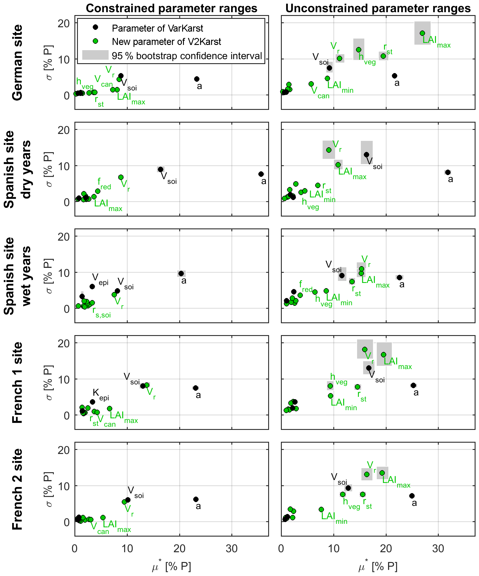
Figure 7 Sensitivity indices of the V2Karst parameters (μ^* is the mean of the absolute elementary effects and σ is the standard deviation of the elementary effects) for total simulated recharge (expressed as a percentage of total precipitation) at the four FLUXNET sites, when constrained (site-specific) parameter ranges are used (ranges of Table 3) and when unconstrained ranges are used (ranges of Table 1). Sensitivity indices were computed over the period from 1 January 2001 to 17 December 2009 for the German site, 1 January 2006 to 31 December 2008 for the Spanish site (dry years), 1 January 2009 to 30 December 2011 for the Spanish site (wet years), 1 January 2010 to 30 December 2011 for the French 1 site and 1 April 2003 to 31 March 2009 for the French 2 site.

5.2 Global sensitivity analysis of the model parameters

The sensitivity analysis results are reported in Fig. 7 and refer to the sensitivity of the total simulated recharge (expressed as a percentage of total precipitation) to the 15 parameters of the V2Karst model. For each parameter, the plots in Fig. 7 report the absolute mean of the elementary effects (μ^*, total effect of the parameters) on the horizontal axis and their standard deviation (σ, degree of linearity of the effect of the parameters) on the vertical axis. In all plots, we observe that the bootstrap confidence intervals of the sensitivity indices are narrow and show little overlap, which gives confidence that the sensitivity results are robust. Similar to the analysis of the simulated fluxes in Sect. 5.1 (Fig. 5), at the Spanish site we present the results for two different time periods with different precipitation amounts.

We first examine the left panels in Fig. 7, which show the sensitivity results when h_veg, r_st, LAI_min, LAI_max, V_r and V_soi are sampled within the constrained ranges (Table 3), while the ranges for other parameters are taken from Table 1. The objective is to inform model calibration in future model applications, as such parameter ranges capture the uncertainty in parameter values left after considering site-specific information. We first note that μ^* and σ take a non-zero value for all parameters at all sites, which means that all parameters are influential and have a non-linear effect on recharge, possibly through interactions with other parameters.

We observe that the spatial variability coefficient a has the largest influence by far, followed by the V_soi and V_r parameters. In fact, their value of μ^* is significantly higher than the other parameters at all sites. The implication for model calibration in future applications of V2Karst is that efforts should primarily seek to reduce the uncertainty in a, V_soi and V_r parameters. These three parameters also have a significantly large value of σ, which indicates non-linearities in the model response to variations in these parameters. Interestingly, V_can, which controls evaporation from interception, has an impact on recharge at most sites, and r_s,soi, which controls soil evaporation, has an impact on recharge at the Spanish site during wet years. This shows that the processes of evaporation from interception and soil evaporation can be important for recharge simulations.

Moreover, we observe that the LAI_min, z₀, k and V_e parameters have a very small impact on total recharge at all sites (${\mathit{\mu }}^{*}<\mathrm{3}$ %). However, Sect. S7 of our Supplement reports additional sensitivity analysis results for other model outputs and shows that the most influential parameters which should be the focus of the calibration strategy vary depending on the output of interest.

We then examine the right panels of Fig. 7, which show the sensitivity indices when sampling parameters within unconstrained ranges (Table 1). This analysis allows one to test the plausibility of the model structure through the assessment of the model sensitivity across a large spectrum of soil and vegetation conditions.

The most apparent difference with respect to the previous results is that vegetation parameters (h_veg, r_st, LAI_min, LAI_max and V_r) now have a much higher value of the sensitivity indices (both μ^* and σ). More specifically, LAI_max has a very high sensitivity index at all sites (${\mathit{\mu }}^{*}>\mathrm{10.5}$ %), which can be attributed to the fact that this parameter is used to calculate different model components. Interestingly, the seasonality of the LAI appears to play an important role in V2Karst as μ^* for LAI_min, although always lower than μ^* for LAI_max, stands out at all sites.

The considerable variations in parameter sensitivities observed across sites can be interpreted by considering their climatic differences. We would expect transpiration to be mainly energy-limited at the German site, given that it has a suboceanic–submountain climate; in contrast, we would expect it to be mainly water-limited at the French sites, which have a Mediterranean climate, and at the Spanish site, which has a semi-arid Mediterranean climate. In this regard, the most influential parameter at the Spanish site is by far the a parameter (high μ^*), which has an impact on the water storage in the soil and therefore on the amount of water available to sustain ET between rain events, while at the German site, parameters r_st and h_veg, which control PET, are more influential compared to the other sites.

Finally, we observe that, the parameters that specifically control the volume of transpiration (r_st and V_r) have a significantly higher value of μ^* than the parameters that specifically control soil evaporation (z₀, r_s,soi and V_e) and evaporation from interception (V_can). Moreover, z₀, r_s,soi and V_e have a very small impact (${\mathit{\mu }}^{*}<\mathrm{3}$ %), while parameter V_can can have an important effect at the German site (${\mathit{\mu }}^{*}=\mathrm{5.7}$ %). Additionally, we see that parameter f_red, which controls transpiration from the third soil layer, has an impact on recharge simulated at the Spanish site.

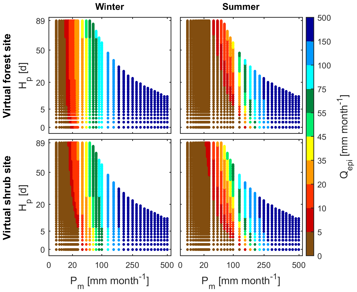
Figure 8 Average monthly recharge (Q_epi) simulated with V2Karst for different values of average monthly precipitation P_m (mm month⁻¹) and the interval between wet days H_p (days) of the synthetic periodic precipitation input used to force the model, at the virtual forest and shrub sites and under winter and summer conditions.

5.3 Virtual experiments

After showing that the V2Karst model behaves reasonably at the four FLUXNET sites, in this section we use virtual experiments to further learn about the sensitivity of simulated recharge to precipitation characteristics and land cover using virtual sites (see Sect. 4.3). Figure 8 shows the monthly average value of simulated recharge Q_epi, for a range of synthetic precipitation inputs with different values of the precipitation monthly amount P_m (x axis) and of the interval between rainy days H_p (y axis) at the virtual forest and shrub sites. We do not report Q_epi values in the top right of the plots because this region corresponds to very intense precipitation events (higher than 200 mm d⁻¹) that have a very low probability of occurrence (see Sect. 4.3).

From the top left panel of Fig. 8, we see that winter Q_epi is mostly sensitive to P_m, in fact simulated recharge increases along the x axis from left to right but shows little variations along the y axis (when H_p is varied). This result is due to the fact that the actual ET is very limited in winter because of the low energy available. We indeed estimated that the maximum value of total ET across the different precipitation inputs is 13 mm month⁻¹ at the forest site and 35 mm month⁻¹ at the shrub site. Therefore, a large part of precipitation becomes recharge rather independently of its temporal distribution.

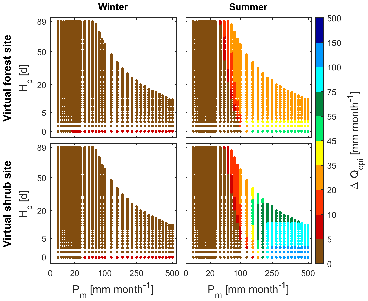
Figure 9 Change in monthly recharge ($\mathrm{\Delta }{Q}_{\text{epi}}=Q_{\text{epi}}^{\text{shrub}}-Q_{\text{epi}}^{\text{forest}}$) simulated with V2Karst when the land cover is set to shrub compared to forest for different values of average monthly precipitation P_m (mm month⁻¹) and the interval between wet days H_p (days) of the synthetic periodic precipitation input used to force the model, at the virtual forest and shrub sites and under winter and summer conditions.

From the right panel of Fig. 8, we observe a systematic reduction in summer Q_epi compared to winter at both virtual sites. Moreover, summer recharge is generally highly sensitive not only to P_m but also to H_p, as it increases when moving along the y axis from bottom to top, i.e. when the same amount of monthly precipitation falls in less frequent but more intense events. This result can be explained by the fact that in summer potential ET is larger and therefore, if events are less intense, a larger part of the precipitation is lost via ET. In contrast, if events are more intense, the canopy and soil stores reach saturation. In this case, a saturation excess flow to the epikarst is generated – hence, there is more recharge and less ET. Moreover, in summer, Q_epi shows a limited sensitivity to P_m and H_p when these quantities take low values (brown and red dots on the left of the plots). This is due to the fact that only a few soil compartments reach saturation under drier conditions and therefore little recharge can be generated. We also note that Q_epi is a significant flux (Q_epi>5 mm) for smaller values of P_m and H_p at the shrub site compared to the forest site. This may be due to the fact that the soil water capacity (V_soi) is much smaller at the shrub site, and the soil compartments can therefore reach saturation under drier conditions.

Finally, Fig. 9 reports the results of another virtual experiment which is focused on the impact of land cover change. Specifically, the panels in Fig. 9 show the variation in simulated recharge when land cover is changed from forest to shrub at the virtual forest site (and vice versa at the virtual shrub site), and more specifically, Fig. 9 reports $\mathrm{\Delta }{Q}_{\text{epi}}=Q_{\text{epi}}^{\text{shrub}}-Q_{\text{epi}}^{\text{forest}}$. We see that in all plots ΔQ_epi is positive, which means that recharge is larger and actual ET is lower under shrub land cover compared with forest land cover for both sites. From the left panels of Fig. 9, we observe that ΔQ_epi is very limited in winter, which is expected as ET fluxes are small in winter as explained above.

Conversely, the right panels of Fig. 9 show that summer ΔQ_epi is much higher than in winter conditions and is sensitive to both P_m and H_p. The sensitivity of ΔQ_epi is highly variable across the different precipitation inputs, and more specifically an increase in H_p can have a different effect on ΔQ_epi depending on the value of P_m (no variation, increase or decrease in ΔQ_epi). In fact, when P_m is low, ΔQ_epi is always low and does not vary sensibly when P_m and H_p are varied (brown area in the left end of the plot), since recharge is always low under these precipitation conditions as shown in Fig. 8. For intermediate values of P_m, ΔQ_epi has a similar pattern at both sites and increases when either H_p or P_m increases. Instead, for high values of P_m, we see that for both sites ΔQ_epi decreases when H_p increases. ΔQ_epi is largest when the monthly precipitation P_m is high and the interval between wet days H_p is low (green dots at the virtual forest site and dark blue dots at the virtual shrub site), because under these precipitation conditions the amount of moisture available for ET is maximum.

Importantly, our results also show that the impact of a change in land cover can vary greatly across sites, as at the virtual shrub site summer ΔQ_epi reaches much higher values and is sensitive to P_m and H_p over a larger range of values of P_m and H_p compared to the virtual forest site.

6 Discussion

6.1 Plausibility of V2Karst simulations against site specific information

We tested the model by evaluating its ability to reproduce observations at four carbonate rock FLUXNET sites, which is a standard approach to model testing, used for instance to test the previous version of the model VarKarst (Hartmann et al., 2015) and large-scale ET products (Martens et al., 2017; McCabe et al., 2016; Miralles et al., 2011). We demonstrated that V2Karst is able to produce behavioural simulations consistent with observations and a priori information at FLUXNET sites. In addition, the time series of simulated water balance components are coherent with our understanding of the sites. A different number of behavioural parameterisations was identified at the different sites, with the highest number found at the more humid German site and the lowest number at the semi-arid Spanish site, which is coherent with previous findings that a better fit to observations can be obtained at wetter locations (Atkinson et al., 2002; Bai et al., 2015).

Interestingly, the behavioural parameter sets for the French 1 site corroborate the hypothesis that root water uptake is likely to extend below the physical soil layer, as communicated by Guillaume Simioni (investigator of the site). In fact, we found behavioural values of the V_r parameter above 59 mm, while site-specific information indicates that the physical soil layer has a storage capacity of 49 mm (Table B1). This result further attests to the realism of V2Karst structure.

The results of the global sensitivity analysis of simulated recharge to the model parameters are easily interpreted in light of the different climatic conditions at the four FLUXNET sites. Parameters that control PET and the soil water storage capacity generally have a large impact on simulated recharge. The interception capacity is also very important at the German site. These findings are in line with the few sensitivity analysis studies of large-scale hydrological models (Güntner et al., 2007; Werth et al., 2009), which have examined the sensitivity of continental water storage and river discharge simulated by the WaterGAP model. The importance of the maximum leaf area index and, to a lesser extent, of the seasonality of vegetation in the V2Karst model is also consistent with previous studies. For example, Tesemma et al. (2015) found that assimilating year-to-year monthly LAI in the VIC model can significantly improve runoff simulations compared with using long-term average LAI; furthermore, Rosero et al. (2010) determined that LAI has a large influence on simulated latent heat in the Noah land surface model. Therefore, our sensitivity analysis results generally suggest that the model behaves sensibly and consistently with our understanding of the key vegetation–recharge processes that we aim to reproduce.

6.2 Sensitivity of simulated groundwater recharge to changes in climate and vegetation characteristics

Our results also provide valuable insights about possible vulnerabilities of karst systems. For example, the fact that the LAI is a highly influential parameter at all FLUXNET sites suggests that the increasing trend in global LAI documented by Zhu et al. (2016) could be reflected as a significant impact on groundwater recharge and on the partitioning between green and blue water in karst areas.

Variations in simulated recharge were also systematically examined under combined changing land cover type and climate conditions (precipitation overall amount and temporal distribution), as the model should be appropriate for climate and land cover change impact studies. We used virtual experiments with synthetic data because they allow one to unequivocally attribute changes in recharge to changes in climate and land cover. Importantly, we showed that precipitation characteristics and land cover have an interacting effect on simulated recharge; these findings are consistent with the global and observational analysis by Kim and Jackson (2012) of non-karst areas, which revealed interactions among vegetation and climate (in particular the overall amount of precipitation) in producing recharge. We found that simulated recharge is lower (and ET is higher) for forest than for the shorter vegetation type considered, i.e. shrubs, which is in line with expectations and with previous studies undertaken in karst areas (Ford and Williams, 2007; Williams, 1993). We demonstrated that the overall amount and daily intensity of precipitation have a positive effect on simulated recharge, i.e. the higher these factors are the higher the recharge. This is consistent with previous observational studies, which found that heavy precipitation events enhance groundwater recharge in non-karst areas (e.g. Taylor et al., 2013, in a semi-arid tropical region; Owor et al., 2009, in a seasonally humid tropical region). Conversely, the modelling study by Hartmann et al. (2017) showed that heavy precipitation events can have a negative effect on recharge simulated by the VarKarst model in some carbonate rock areas in Europe, the Middle East and northern Africa. However, Hartmann et al. (2017) analysed the sensitivity of simulated recharge using forcing data from global circulation models (GCMs). Given that climate variables from GCMs show complex patterns, it might be difficult to isolate the effect of a specific climate property (e.g. heavy precipitation events) on the simulated fluxes, which could explain the differences between their findings and ours.

Precipitation patterns are more complex than the simple periodic variations we used here, and the steady-state conditions may never be reached in practice. Nevertheless, we believe that performing virtual experiments similar to those proposed in the present study is a complementary approach to the application of climate projections provided by GCMs and future land cover change scenarios (e.g. Holman et al., 2017; Hurtt et al., 2011), to systematically assess the sensitivity of a model to changes in input characteristics, to test the soundness of the model sensitivities and to determine which aspects of a model input would be worth further investigating.

6.3 Applying V2Karst over larger domains

The results of our global sensitivity analyses suggest that all newly introduced processes in V2Karst are relevant for applications over large domains because the parameters that control these processes can affect simulated recharge, depending on the climatic, soil and land cover conditions. Specifically, transpiration and vegetation seasonality are important processes under the climate of the four FLUXNET sites, evaporation from canopy interception is important at all forested sites (German site and two French sites), the contribution of water stored below the root zone is important under the climate of the Spanish site and soil evaporation is important at the semi-arid site with sparse and short vegetation (Spanish site). The significance of representing canopy interception, in particular for forested land covers, has already been mentioned in previous studies (Gerrits, 2010; Savenije, 2004), whilst the importance of separating transpiration and soil evaporation was reported in Maxwell and Condon (2016) and Wang and Dickinson (2012).

Regarding parameter estimation, the use of soft rules similar to this study and to the large-scale study of Hartmann et al. (2015) can be envisaged for applications over large domains. We showed that a priori information on parameter ranges is needed to constrain the simulations. At large scales, a priori information on vegetation parameters can be derived from large-scale databases of vegetation properties (more details in Sect. S1 of our Supplement), and a priori information on parameters that control the subsurface properties (V_soi) can be derived following Hartmann et al. (2015). It is also particularly important to assess the sensitivity of model parameters across the modelling domain to test the suitability of fixing model parameters, as done in this study at FLUXNET sites. We indeed found that parameters V_can and r_s,soi, which are typically fixed in the other large-scale models detailed in Table A1, do have an impact on simulated recharge at least one FLUXNET site. Moreover, as mentioned in Sect. 2.3, V_can and r_s,soi are understood to vary across land cover types and soil types, respectively, even if no clear ranges of these parameters have been established across either land cover or soil types. Therefore, fixing these two parameters could potentially introduce large uncertainties in V2Karst simulations. Other studies have reported on this issue; Cuntz et al. (2016), in particular, showed that some constant parameters of the Noah-MP land surface model can be highly influential for some model outputs. Finally, parameter estimation for applications over large domains will need to account for the large variability in hydraulic properties and recharge patterns observed across karst systems reported, for example, in Hartmann et al. (2014) and Klimchouk and Ford (2000), for instance using a simplified classification of karst landscapes based on climate and topography as in Hartmann et al. (2015).

We note that although soils may be absent in some karst areas (e.g. karren field in high mountain areas as reported in Hartmann et al., 2014), V2Karst always includes a soil layer. However, this soil layer can be very thin and has a limited impact on recharge. Additionally, when the simulation units have a large extent, such as $\mathrm{0.25}{}^{\circ }\times \mathrm{0.25}{}^{\circ }$ in Hartmann et al. (2015), it is reasonable to assume that soil layers can always be found.

The V2Karst model can account for the sub-grid heterogeneity in the vegetation type using a “tile” approach as in Mac-PDM (Gosling and Arnell, 2011) and VIC (Bohn and Vivoni, 2016), which consists of subdividing each model grid cell into a number of independent units (tiles), each of which has a specific land cover (e.g. short or tall vegetation). The model is then evaluated separately over each tile and the overall simulated fluxes are computed as the area weighted average of the fluxes calculated over the tiles. In V2Karst, each “tile” includes a vegetated and non-vegetated fraction as explained in Sect. 2.3.3.

The V2Karst model implements a simplified representation of ET and karst processes, given the limited amount of data available at large scales as discussed in Sect. 2.1. In particular, further information on typical karstic features over large domains would be valuable to refine the representation of karst processes in V2Karst in future developments of the model, to consider additional processes explicitly (the formation of a perched aquifer in the epikarst, which can occur in highly weathered karst systems as described e.g. in Williams (1983, 2008); this process is represented e.g. in a previous karst model developed for applications at the local scale introduced in Hartmann et al., 2012b).

7 Conclusions

The objectives of the present study were (1) to develop and test an ET component with the explicit representation of land cover processes for the karst recharge model VarKarst, so that the model can be used for combined climate and land cover change impact assessment at large scales, and (2) to evaluate the mechanisms of recharge production in the model as well as the model sensitivity to temporal precipitation patterns and land cover using observations and synthetic data to force the model.

Many different approaches are used to represent ET in large-scale hydrologic models, and the lack of in situ ET observations makes it difficult to assess and compare the performance of these different formulations. Moreover, some models use a large number of parameters that can only be poorly constrained by the few available observations. High model complexity also makes Monte Carlo simulation computationally expensive and hampers uncertainty and sensitivity analysis. The new version of the VarKarst model developed here, V2Karst (V1.1), is the first large-scale hydrological model to include explicit representations of both karst and land cover processes. We sought to include parsimonious process descriptions that are understood to be relevant for climate and land cover impact assessment, namely, (1) a representation of the three ET components (transpiration, soil evaporation in presence of sparse canopy and evaporation from canopy interception) and (2) a physically based PET equation (Penman–Monteith). The model also comprises a parsimonious representation of vegetation seasonality.

We demonstrated that V2Karst produces credible simulations at four carbonate rock FLUXNET sites, by showing that it reproduces observations of latent heat and soil moisture and that the parameters which dominate the model sensitivity are in accordance with our perception of expected controls on recharge. We also established that the model has plausible sensitivities to climate and land cover changes when using virtual experiments with synthetic precipitation and land cover scenarios. Additionally, we showed that the newly introduced processes in V2Karst can have varying impacts on simulated recharge quantities depending on the climate, the soil properties and the land cover.

Overall, our study demonstrates the value of a model development and evaluation process that considers both how well a model reproduces historical observations as well as how this performance is achieved. The latter is examined using global sensitivity analysis to understand which processes and inputs dominate the model output. Through the proposed process we have a higher chance of obtaining the right results for the right reasons than we would have using performance analysis alone (Kirchner, 2006). We further believe – given the lack of observations of many hydrological fluxes at large scales – that an integrated analysis using historical data, our expectations derived from previous studies and synthetic data (to understand model behaviour more generally) can provide a more holistic view of a model than using observations alone.

Appendix A: Review of ET component in large-scale hydrological models

Table A1 Characteristics of selected large-scale models: simulation time step (Δt), representation of sub-grid variability of soil moisture, solving of the energy balance, ET processes represented (overstorey transpiration $T_{\text{act}}^{\text{over}}$, understory transpiration $T_{\text{act}}^{\text{under}}$, soil evaporation Es_act, evaporation from canopy interception Ec_act and carbon cycle i.e. vegetation dynamic model), and number of parameters for ET estimation. The models were selected based on the following criteria: (1) explicit representation of land cover properties, (2) calculation of ET and soil water balance at a daily or sub-daily time step, and (3) applications in previous studies over a wide range of climate and land cover types. Tables A2 and A3 present the parameterisations used in these models, while a detailed list of all parameters involved in the representation of ET in these models can be found in Sect. S2 of our Supplement.

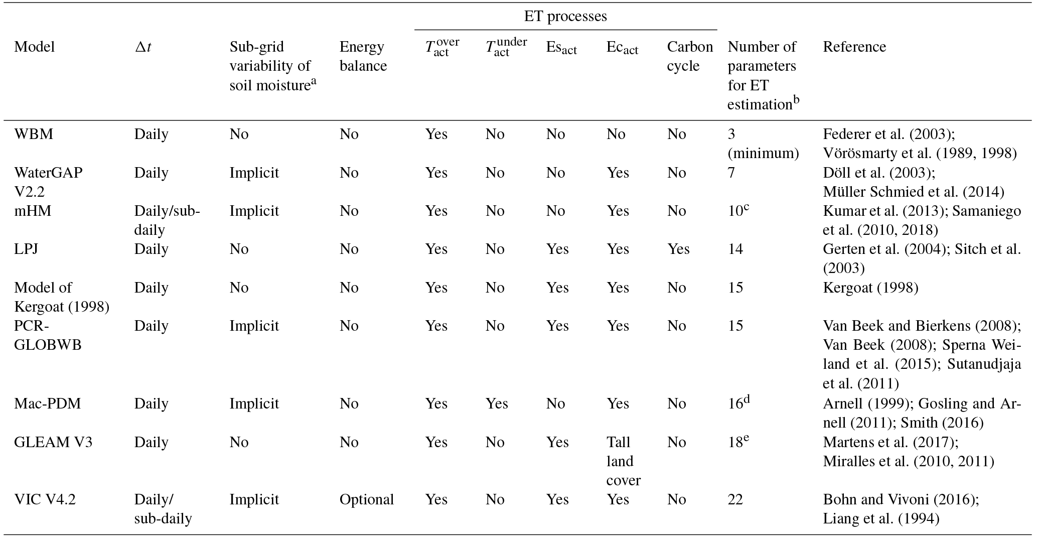
^a None of these models account for karst processes as done by the VarKarst model (Hartmann et al., 2015). ^b Number of parameters for a given land cover type, excluding parameters used in the representation of vegetation seasonality, carbon cycle (vegetation dynamic), sublimation from snowpack and snowmelt evaporation to make models more comparable. ^c Number of parameters considering three soil layers. ^d This number includes the parameters used for the computation of both understory and overstorey (grass) transpiration. ^e Number of parameters assuming tall vegetation (interception is considered for tall vegetation only).

Table A2 Representation of potential evapotranspiration (PET) and stress model for actual evapotranspiration (ET) calculation from PET in the large-scale models of Table A1.

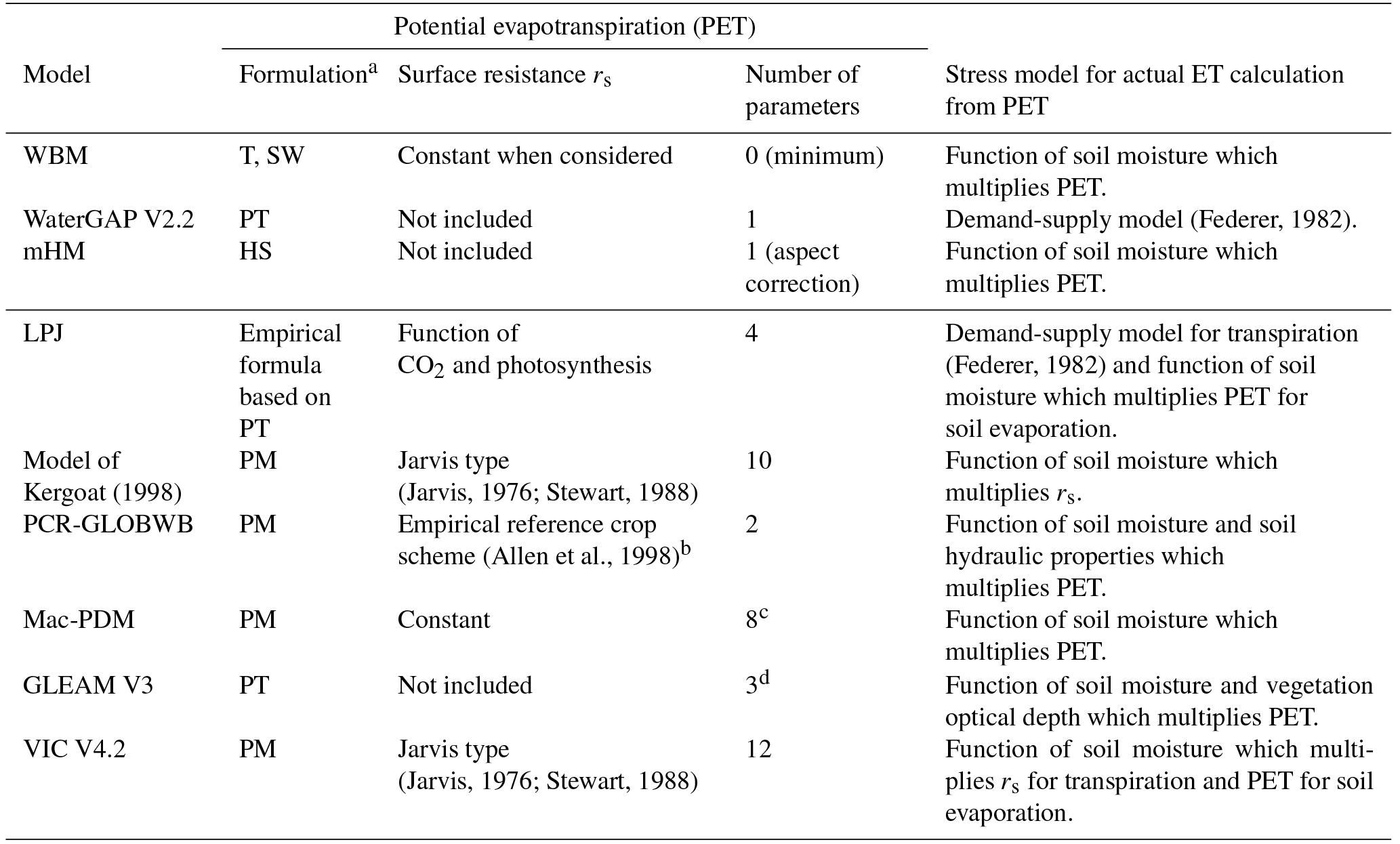
^a T: Thornthwaite (1948); HS: Hargreaves and Samani (1985); PT: Priestley–Taylor (1972); PM: Penman–Monteith (Monteith, 1965); SW: Shuttleworth and Wallace (1985). ^b This approach consists of calculating a value of PET for a reference grass surface with known properties and to adjust this potential rate using land cover specific empirical crop factors. This formulation avoids the specification of the stomatal resistance whose value is largely uncertain (see Sect. S1 of our Supplement). Tabulated values of the crop factors for agricultural crops are provided in Allen et al. (1998). However, the origin of the crop factor formulation for non-agricultural crops is not clear. ^c This number includes the parameters used for the computation of PET for both understory and overstorey (grass). ^d Number of parameters assuming tall vegetation (interception is considered for tall vegetation only).

Table A3 Representation of sparse vegetation, soil layers, evaporation from canopy interception and seasonality of vegetation in the large-scale models of Table A1.

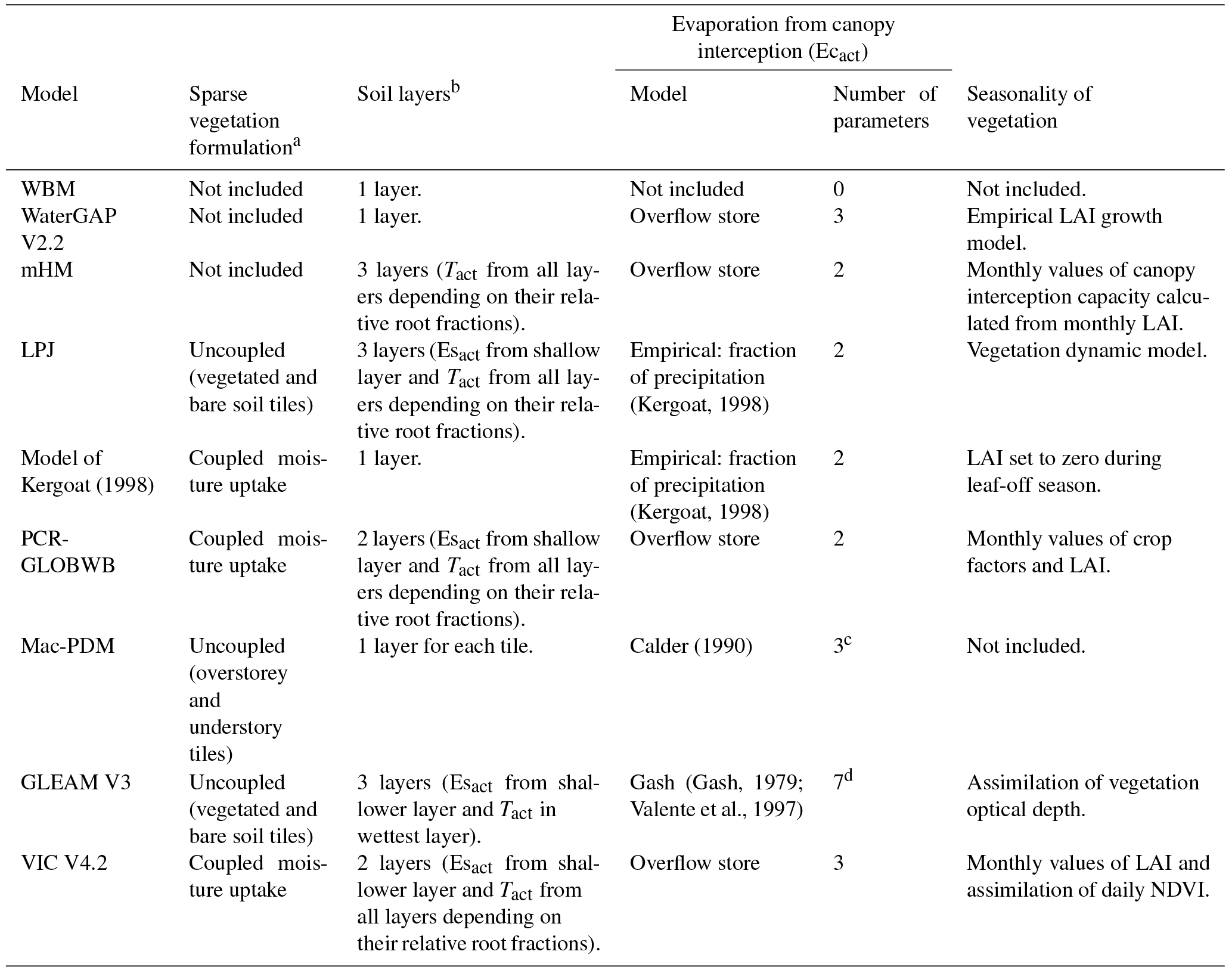
^a Uncoupled approaches consist of separately assessing the water balance for the vegetated and bare soil fractions (overstorey and understory fractions for Mac-PDM). Therefore, this approach is based on the simplifying assumption that the vegetation roots do not extent beyond the surface area covered by the vegetation canopy. Instead, coupled approaches evaluate the overall water balance over both fractions, thus allowing for interactions for soil moisture uptake between vegetated and bare soil fractions. All models neglect aerodynamic interactions between vegetation and bare soil. This can be accounted for using for instance the Shuttleworth–Wallace PET equation (Shuttleworth and Wallace, 1985), which requires the specification of further resistance parameters compared to the Penman–Monteith equation. The Shuttleworth–Wallace equation was used anecdotally in the WBM model for a few applications. ^b Es_act: actual soil evaporation; T_act: actual vegetation transpiration. ^c This number includes the parameters used for the computation of PET for both understory and overstorey (grass). ^d Number of parameters assuming tall vegetation (interception is considered for tall vegetation only).

Appendix B: Additional information on the four carbonate rock FLUXNET sites

Table B1 Description of the four carbonate rock FLUXNET sites.

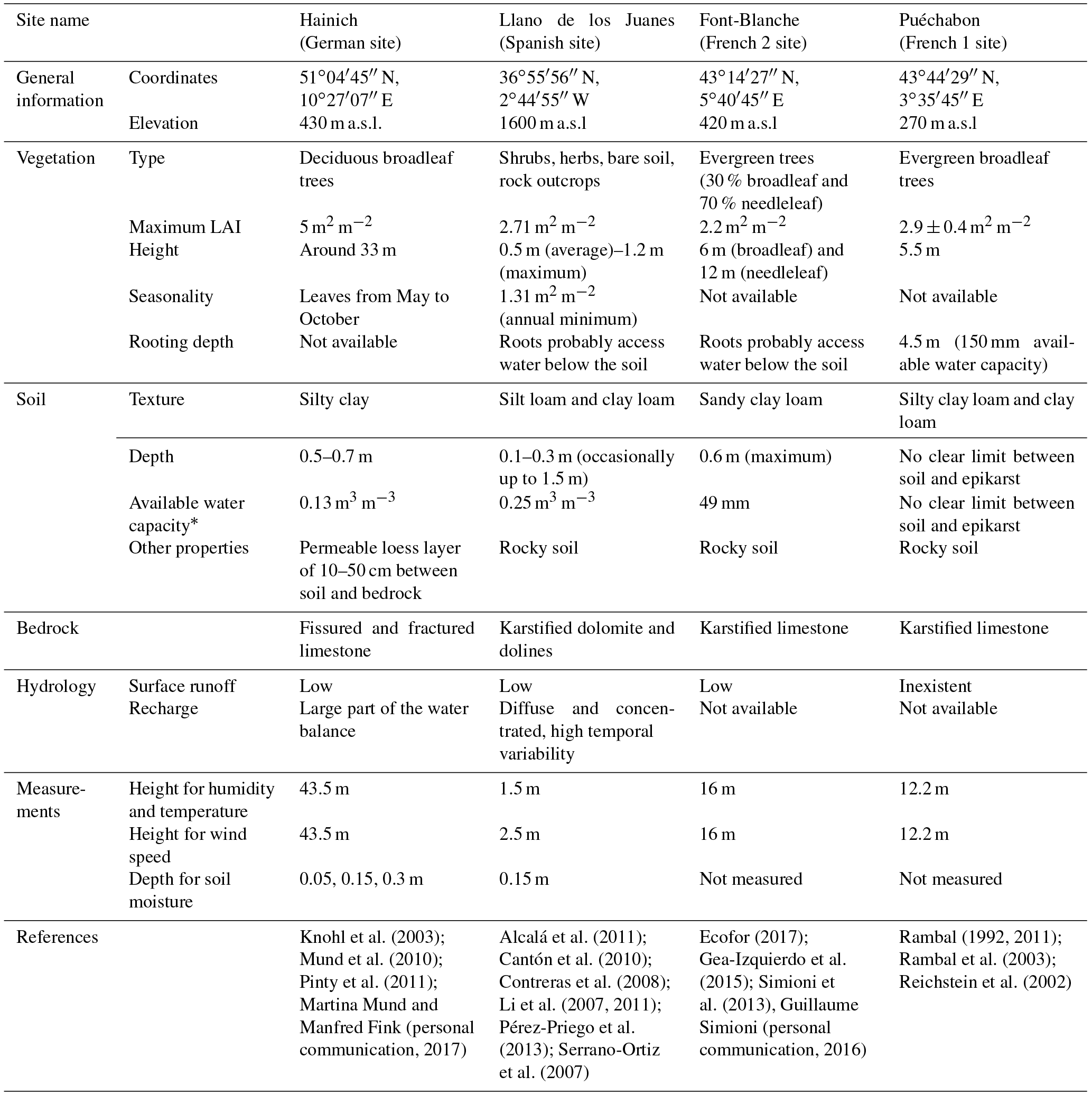
^* Between wilting point and field capacity.