the Creative Commons Attribution 4.0 License.
the Creative Commons Attribution 4.0 License.
 | 10 Oct 2018
Comparison of dealiasing schemes in large-eddy simulation of neutrally stratified atmospheric flows
Fabien Margairaz
Marco G. Giometto
Marc B. Parlange
Marc Calaf
Aliasing errors arise in the multiplication of partial sums, such as those encountered when numerically solving the Navier–Stokes equations, and can be detrimental to the accuracy of a numerical solution. In this work, a performance and cost analysis is proposed for widely used dealiasing schemes in large-eddy simulation, focusing on a neutrally stratified, pressure-driven atmospheric boundary-layer flow. Specifically, the exact 3∕2 rule, the Fourier truncation method, and a high-order Fourier smoothing method are intercompared.
Tests are performed within a newly developed mixed pseudo-spectral finite differences large-eddy simulation code, parallelized using a two-dimensional pencil decomposition. A series of simulations are performed at varying resolution, and key flow statistics are intercompared among the considered runs and dealiasing schemes.
The three dealiasing methods compare well in terms of first- and second-order statistics for the considered cases, with modest local departures that decrease as the grid stencil is reduced. Computed velocity spectra using the 3∕2 rule and the FS method are in good agreement, whereas the FT method yields a spurious energy redistribution across wavenumbers that compromises both the energy-containing and inertial sublayer trends. The main advantage of the FS and FT methods when compared to the 3∕2 rule is a notable reduction in computational cost, with larger savings as the resolution is increased (15 % for a resolution of 1283, up to a theoretical 30 % for a resolution of 20483).
- Article
(5473 KB) - Full-text XML
- BibTeX
- EndNote


The past decades have seen significant progress in computer hardware in remarkable agreement with Moore's law, which states that the number of nodes in the discretization grids doubles every 18 months (Moore, 1965; Takahashi, 2005; Voller and Porté-Agel, 2002). A comparable progress has been made in software development, with the rise of new branches in numerical analysis like reduced-order modeling (Burkardt et al., 2006) and uncertainty quantification (Najm, 2009), as well as the development of highly efficient numerical algorithms and computing frameworks like isogeometric analysis (Hsu et al., 2011) or GPU computing (Bernaschi et al., 2010; Hamada et al., 2009)
At the same time, with increasing computer power, the range of scales and applications in computational fluid dynamics (CFD) has significantly broadened, allowing us to describe – at an unprecedented level of detail – complex flow systems such as fluid–structure interaction (Bernaschi et al., 2010; Hughes et al., 2005; Takizawa and Tezduyar, 2011), land–atmosphere exchange of scalars, momentum and mass (Albertson and Parlange, 1999; Anderson et al., 2012; Bou-Zeid et al., 2004; Calaf et al., 2010; Giometto et al., 2016, 2017; Moeng, 1984), weather research and forecasting (Skamarock et al., 2008), micro-fluidics (Wörner, 2012), and canonical wall-bounded flows (Schlatter and Örlü, 2012), to name but a few. Despite this progress, high-resolution simulations effectively exploiting current hardware and software capabilities (i.e., following Moore's law) are challenging as they require significant computational resources, which most research groups do not have at their disposal (Bou-Zeid, 2014). As a result, methods that aim at reducing computational requirements while preserving numerical accuracy are still of great interest.
The Fourier-based pseudo-spectral collocation method (Canuto et al., 2006; Orszag, 1970; Orszag and Pao, 1975) remains the preferred “workhorse” in simulations of wall-bounded flows over horizontally periodic regular domains. This is often used in conjunction with a centered finite-difference or Chebychev polynomial expansions in the vertical direction (Albertson, 1996; Moeng and Sullivan, 2015). The main strength of such an approach is the high order of accuracy of the Fourier partial sum representation, coupled with the intrinsic efficiency of the fast Fourier transform algorithm (Cooley and Tukey, 1965; Frigo and Johnson, 2005). In such algorithms, the leading-order error term is represented by the aliasing that arises when evaluating the quadratic nonlinear term (convective fluxes of momentum). This was first discovered in the early works of Orszag and Patterson (Orszag, 1971; Patterson, 1971), which also set a cornerstone in the treatment and removal of aliasing errors in pseudo-spectral collocation methods. Aliasing errors can severely deteriorate the quality of the solution, as exemplified by the large body of literature that has dealt with the topic. In Horiuti (1987) and Moin and Kim (1982), it was shown how the energy-conserving rotational form of the large-eddy simulation (LES) equations performed poorly without dealiasing and that the proper removal of such error significantly improved the accuracy of the solution in statistics like the flow turbulent shear stress, turbulence intensities, and two-point correlations. As shown in Moser et al. (1983), Zang (1991), and Kravchenko and Moin (1997), aliasing errors do not alter the energy conservation properties of the rotational form of the LES equations, but the additional dissipation that is introduced makes the flow prone to laminarization. Dealiasing is hence required in order to accurately resolve turbulent flows with a well-developed inertial subrange, such as atmospheric boundary layer (ABL) flows, for instance. However, the classic (exact) dealiasing methods developed in Patterson (1971) based on padding and truncation (the 3∕2 rule) or on the phase-shift technique have proven to be computationally expensive and are one of the most costly modules for momentum integration in high-resolution simulations, as it will be shown later in this work. For example, in simulations with Cartesian discretization, where N is the number of collocation nodes in each of the three coordinate directions, the 3∕2 rule requires us to expand the number of nodes to , and the phase-shift method needs grids with 2×N nodes. As a result, the computational burden introduced by these methods is high, mainly due to the nonlinear increase in the cost of the fast Fourier transform algorithm (such as the one implemented in the Fastest Fourier Transform in the West (FFTW) library). Additionally, this cost rises more rapidly when the Fourier transform is performed in higher dimensions. Therefore, the treatment of aliasing errors severely limits the computational performances of large-scale models based on high-order schemes.
This has motivated efforts towards the development of approximate yet computationally efficient dealiasing schemes, such as the Fourier truncation (FT) method (Moeng, 1984; Moeng and Wyngaard, 1988; Orszag, 1971), the Fourier smoothing (FS) method (Hou and Li, 2007), and the more recent implicit dealiasing of Bowman and Roberts (2011). Details on the FT and the FS techniques are provided in the following section. Limits and merits of the different dealiasing techniques have been extensively discussed in the past decades within the turbulent flow framework (Moser et al., 1983; Zang, 1991).
In this work, we provide a cost–benefit analysis and a comparison of turbulent flow statistics for the FT and FS dealiasing schemes in comparison to the exact 3∕2 rule using a set of LES of fully developed ABL-type flows. Simulations and benchmark analysis are performed using a recently developed mixed pseudo-spectral finite difference code, parallelized via a pencil decomposition technique based on the 2DECOMP&FFT library (Li and Laizet, 2010). Results of this work are of prime interest to the environmental fluids community (e.g., ABL community) because they can help improve the numerical performance of some of the numerical approaches used. An overview of the different dealiasing methods is provided in Sect. 2. Section 3 briefly presents the LES platform with important benchmark results. The computational cost analysis and flow statistics obtained with the different dealiasing schemes are later discussed in Sect. 4. Finally, the conclusions are presented in Sect. 6.
Aliasing errors result from representing the product of two or more variables by N wavenumbers, when each one of the variables is itself represented by a finite sum of N terms (Canuto et al., 2006); here, N is assumed even. Such is the case for example when treating the nonlinear advection term in the Navier–Stokes (NS) equations. Let f and g be two smooth functions with the corresponding discrete Fourier transforms expressed as
with and being the amplitudes of the kth Fourier mode of f and g. The product of the two functions is hence given by
with
Note that the corresponding expression for the Fourier transform of the product h (result of the convolution of f with g) requires 2N modes. Therefore, the exact computation of the product represents a major numerical cost. Traditionally the convolution of the two functions f and g is made with only N Fourier modes,
As a result, the energy contained within the remaining N+1 to 2N modes folds back on the first N modes, and the amplitude of the first N modes () is aliased. This can be related to the exact amplitude as
with
such that the second term contains the aliasing errors on the kth mode. Aliasing errors propagate in the solution of the differential equation and can induce large errors. For the pseudo-spectral methods, the truncation and aliasing errors affect both the accuracy and the stability of the numerical solution (see Canuto et al., 2006, Sect. 3, and Canuto et al., 2007, Sect. 3, for detailed discussion). Traditionally, the aliasing errors are treated using one of the two methods discussed below.
The 3∕2-rule method is based on the so-called padding and truncation technique, where the Fourier partial sums are zero-padded in Fourier space by half the available modes (from N to 3∕2N), inverse-transformed to physical space before multiplication, multiplied, and then truncated back to the original variable size (N). This method fully removes aliasing errors. However, the high computational cost related to the inverse transform operation discourages its use in large-scale simulations. The fast Fourier transform (FFT) algorithm has an operational complexity of Nlog2(N); counting the number of FFT and multiplications, the operation count of the 3∕2 rule applied to dealias the product of two vectors of N components becomes (Canuto et al., 2006). An alternative method is the so-called phase-shift method, which consists of shifting the grid of one of the variables in physical space. Given the appropriate shift, the aliasing errors are eliminated naturally in the evaluation of the convolution sum. This method has a cost equal to 15Nlog2(N) (Canuto et al., 2006), which is even greater than the 3∕2 rule (Orszag, 1972; Patterson, 1971). The discussion above concerns one-dimensional problems, but the expansion to higher-dimensional problems is straightforward (Canuto et al., 2006; Iovieno et al., 2001). Although this method provides the full dealiasing of the nonlinear term, the cost of expanding the number of Fourier modes by a factor of 3∕2 is a computationally expensive endeavor, especially with the progressively increasing size of numerical grids. To reduce the numerical burden, two additional methods were proposed in the past for treating the aliasing errors: the FS method (Hou and Li, 2007), and the FT method (Moeng, 1984; Moeng and Wyngaard, 1988; Orszag, 1971). In both methods, a set of high-wavenumber Fourier amplitudes are multiplied by a test function to avoid expansions to larger number of modes. As its name indicates, the FT method sets to zero the last third of the Fourier modes (f(k)=0, for ), equivalent to a sharp spectral cutoff filter. The FS method consists of a progressive attenuation of the higher frequencies using the weighting function (Hou and Li, 2007). Figure 1 presents the spectral function f(k) for the two different methods. Note that both the FT and FS methods behave like a low-pass filter. Although the FT method (continuous line) sets to zero any coefficient larger than , the FS method (dashed line) keeps all the wavelengths unperturbed up until and then progressively damps the amplitude of the higher-wavenumber terms. The advantage of both of these methods is that they avoid the need for padding the Fourier partial sums and hence reduce the numerical cost. Specifically, the computational cost of these methods is (15∕2)Nlog2(N) (Canuto et al., 2006), resulting in methods 33% less computationally expensive than the 3/2 rule. The drawback of such approximate approaches is, however, the fact that a filtering operation is applied to the advection term, resulting in a loss of information. A desirable property of the FS technique when compared to the FT method is that the former exhibits a more localized error and is dynamically very stable (Hou and Li, 2007), while the latter tends to generate oscillations on the whole domain.
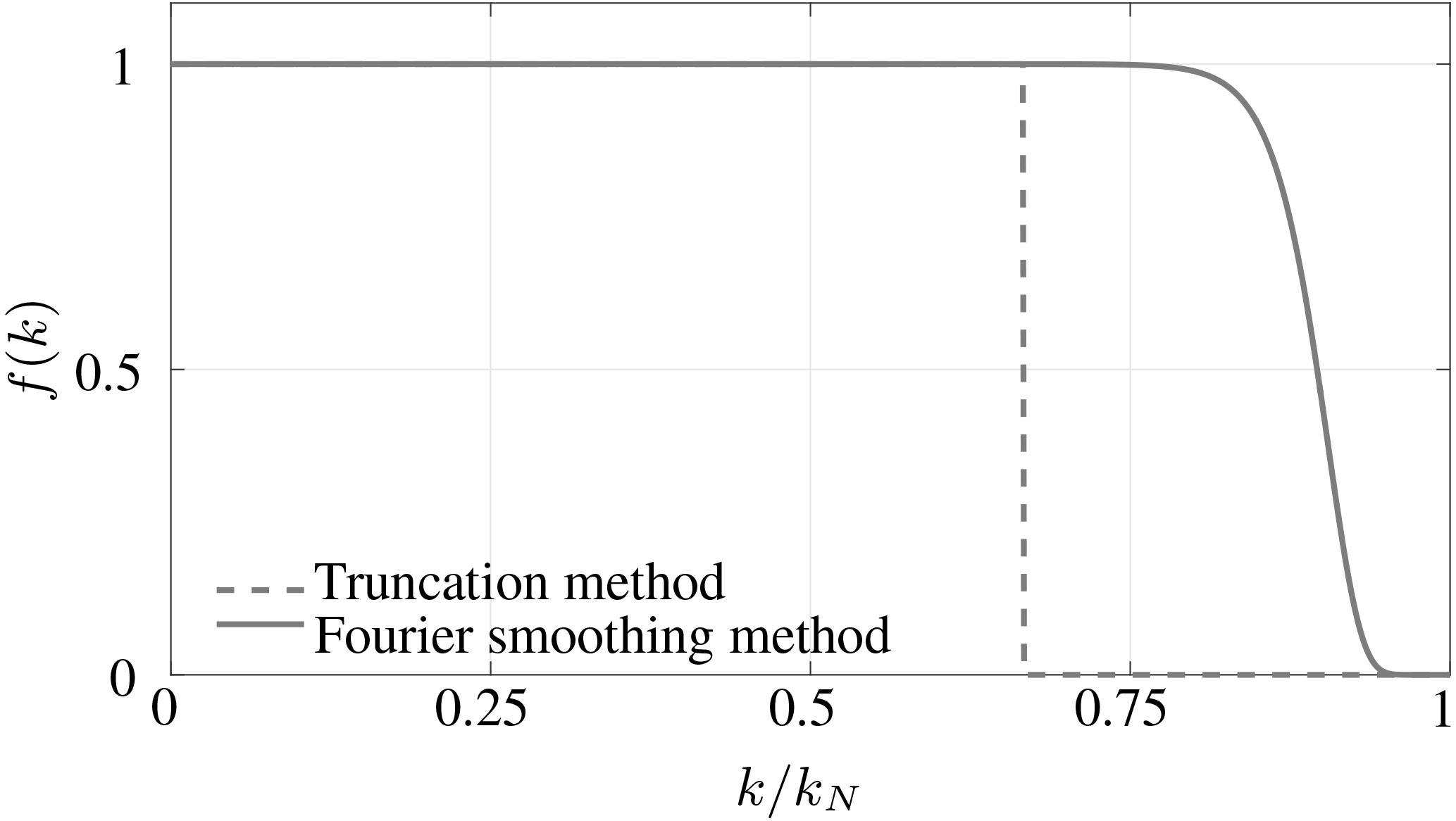
Figure 1Weighting functions used in the FT method (dashed line) and the FS method (continuous line). The FT method filters scales with and the FS method at .
3.1 Equations and boundary conditions
The LES approach consists of solving the filtered NS equations, where the time and space evolution of the turbulent eddies larger than the grid size are fully resolved, and the effect of the smaller ones is parameterized. Mathematically, this is described through the use of a numerical filter that separates the larger, energy-containing eddies from the smaller ones. Often, the numerical grid of size Δ is implicitly used as a top-hat filter, hence reducing the computational cost (see Moeng and Sullivan, 2015, for an overview of the technique in ABL research). As a result, the velocity field can be separated in a resolved component (, where ) and an unresolved contribution () (Smagorinsky, 1963). For this technique to be successful, the low-pass filter operation must be performed at a scale smaller than the energy production range, deep in the inertial subrange according to Kolmogorov's hypothesis (Kolmogorov, 1968; Piomelli, 1999). In atmospheric boundary-layer flow simulations, this requirement is known to hold in the bulk of the flow, where contributions from the sub-grid-scale (SGS) motions (or sub-filter-scale motions) to the overall dissipation rate are modest. In the near-surface regions such a requirement is not met, as the characteristic scale of the energy production range ℒ scales with the distance from the wall (ℒ≈κz, where κ≈0.4 is the Von Kármán constant and z is the wall-normal distance from the wall); hence, this remains an active research field (Hultmark et al., 2013; Lu and Porté-Agel, 2014; Meneveau et al., 1996; Porté-Agel et al., 2000; Sullivan et al., 1994). In this work, the rotational form of the filtered NS equations are integrated, ensuring conservation of mass of the inertial terms (Kravchenko and Moin, 1997). The corresponding dimensional form of the equation reads
In these equations, are the velocity components in the three coordinate directions (streamwise, spanwise, and vertical, respectively), denotes the perturbed modified pressure field defined as , where the first term is the kinematic pressure, the second term is the trace of the sub-grid stress tensor, and the last term is an extra term coming from the rotational form of the momentum equation. Here, represents a generic volumetric force. The flow is driven by a constant pressure gradient in the streamwise direction imposed through the body force . The sub-grid stress tensor is defined as , where the deviatoric components are written using an eddy-viscosity approach
with being the so-called eddy viscosity, the resolved strain rate tensor, and CS the Smagorinsky coefficient, a dimensionless proportionality constant (Lilly, 1967; Smagorinsky, 1963). Many studies have investigated the accuracy of this type of model, showing good behavior for free-shear flows (Lesieur and Metais, 1996). For boundary-layer flows, the Smagorinsky constant model is over-dissipative close to the wall, since the integral length scale scales with the distance to the wall. Therefore, to properly capture the dynamics close to the surface, the Mason–Thompson damping wall function is used (Mason and Thomson, 1992). This function is given by and is used to decrease the value of CS close to the wall, reducing the sub-grid dissipation.
Note that the molecular viscous term has been neglected in the governing equations, including the wall-layer parameterization, which is equivalent to assuming that the surface drag is mostly caused by pressure (i.e., there are negligible viscous contributions). This is a typical situation in flow over natural surfaces where the surface is often in a fully rough aerodynamic regime.
The drag from the underlying surface is entirely modeled in this application through the equilibrium logarithmic law for rough surfaces (Kármán, 1931; Prandtl, 1932), with
In Eq. (10), is the planar averaged velocity sampled at Δz∕2, z0 is the aerodynamic roughness length, representative of the underlying surface, Δz denotes the vertical grid stencil, and κ=0.4 is the von Kármán constant. The wall shear stress is computed considering the norm of the horizontal velocity, and it is projected over the horizontal directions using the unit vector ni, such that , where
In addition, the corresponding vertical derivatives of the horizontal mean velocity field are imposed at the first grid point of the vertically staggered grid (Albertson and Parlange, 1999; Albertson et al., 1995).
This setup has now been extensively used to study neutrally stratified ABL flows (Abkar and Porté-Agel, 2014; Allaerts and Meyers, 2017; Brasseur and Wei, 2010; Cassiani et al., 2008). Moreover, it is used as foundation to build more complex simulations of the ABL adding scalar (passive or active) transport (for example, see Calaf et al., 2011; Saiki et al., 2000; Salesky et al., 2016; Stoll and Porté-Agel, 2008) as well as other physical processes.
3.2 Numerical implementation and time integration scheme
The equations are solved using a pseudo-spectral approach, where the horizontal derivatives are computed using discrete Fourier transforms and the vertical derivatives are computed using second-order accurate centered finite differences on a staggered grid. A projection fractional-step method is used for time integration following Chorin's method (Chorin, 1967, 1968). The governing equations become decoupled, and the system of partial differential equations can be solved in two steps: first, the nonlinear advection–diffusion equation is explicitly advanced, and subsequently the Poisson equation is integrated (the so-called pressure correction step). The latter equation is obtained by taking the divergence of the first equation and setting the divergence of velocity at the next time step equal to zero, to ensure a divergence-free flow field. The algorithm is detailed in the rest of the section. Initially, the code computes the velocity tensor , which contains all the derivatives of the flow field required to compute the SGS stress tensor . In the first step of the projection method, the NS equations are solved without the pressure. Hence, the intermediary right-hand side is computed as
Next, an intermediary step is computed using an Adams–Bashforth scheme, following
where is the right-hand side of the previous step. At this point, the resulting flow field is not divergence-free yet. The modified pressure is used to impose this fundamental property of the flow filed. Therefore, is computed solving the Poisson equation
obtained by taking the divergence of the NS equations. The term on the right-hand side of the equation above is given by
The new flow field for the complete time step is obtained by . Finally, the new right-hand side is updated with the pressure gradient as .
Embedded within this approach, periodic boundary conditions are imposed on the horizontal (x,y) directions. To close the system, a stress-free lid boundary condition is imposed at the top of the domain and an impermeability () condition is imposed at the lower boundary, which sums to the parameterized stress described in Sect. 3.
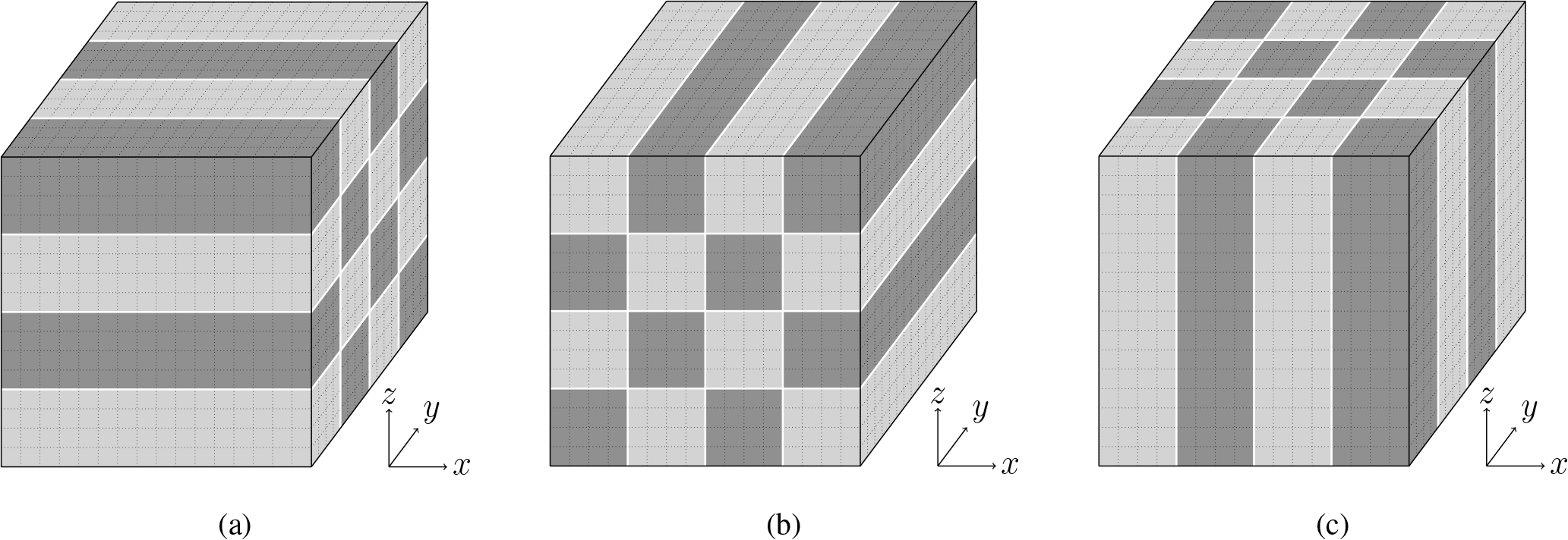
Figure 2Two-dimensional pencil decomposition of the computational domain with the domain transposed into the three direction of space: (a) X pencil, (b) Y pencil, (c) Z pencil (based on Li and Laizet, 2010).
The code is parallelized following a 2-D pencil decomposition paradigm similar to the one presented in Sullivan and Patton (2011), partitioning the domain into squared cylinders aligned along one of the horizontal directions, as shown in Fig. 2. The 2-D pencil decomposition is implemented using the 2DECOMP & FFT open-source library (Li and Laizet, 2010), which shows exceptional scalability up to a large number of message passing interface (MPI) processes (Margairaz et al., 2017).
3.3 Analysis of the numerical cost
The LES algorithm can be separated into four distinct modules: (1) computation of the velocity gradients, (2) evaluation of the SGS stresses and (3) of the convective term, and (4) computation of the pressure field by solving the Poisson equation. These four modules represent the bulk of the computational cost of the code, in addition to MPI communication. Figure 3 presents a simplified flowchart of the main algorithm with each of the four modules.
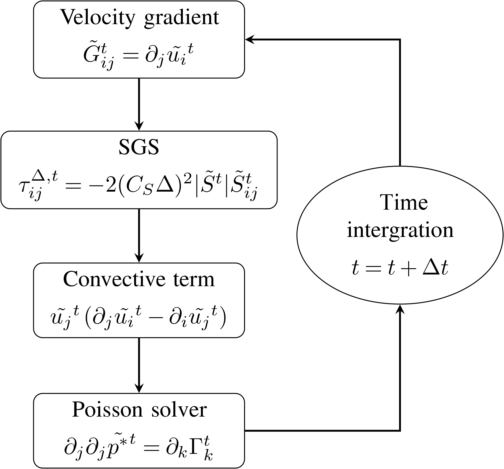
Figure 3Simplified flowchart of the main algorithm presenting the four modules that represent the bulk of the computational cost.
The four modules have been individually timed to evaluate their corresponding computational cost at a resolution of with the 3∕2 rule as a baseline. Results are shown in Fig. 4. As can be observed, more than half of the integration time step (∼60%) is spent computing the convective term. The three other modules share the rest of the integration time as follows: the computation of the velocity gradients (∼20%), the Poisson solver (∼16%), and the SGS (∼4%). It is important to note that this test was conducted without any file input and output as it is not relevant to assess the computational cost of the momentum integration. As explained in Sect. 2, the nonlinear term requires the use of dealiasing techniques to control the aliasing error, which traditionally are associated with a padding operation (as mentioned in Sect. 2) and hence higher computational cost. It is important to note that although the overall integration time distribution between each individual module might vary depending on the numerical resolution employed, the overall cost of the convective term will remain important regardless of the changes in numerical resolution. The goal of this work is to explore the possibility of using alternative dealiasing techniques to enhance the computational performance, while maintaining accurate turbulent flow statistics in simulations of ABL flows. It is important to note that the SGS model used here takes a relatively small fraction of the time integration. This fraction is likely to be larger if a more sophisticated model is used, for example the dynamic Smagorinsky model (Germano et al., 1991) or the Lagrangian scale-dependant model (Bou-Zeid et al., 2005). In addition, it is important to note that the low computational cost of the Poisson solver is related to the use of pencil decomposition, which takes full advantage of the pseudo-spectral approach. Specifically, the Z pencil combines with the horizontal treatment of the derivatives to make the implementation of the solver very efficient.
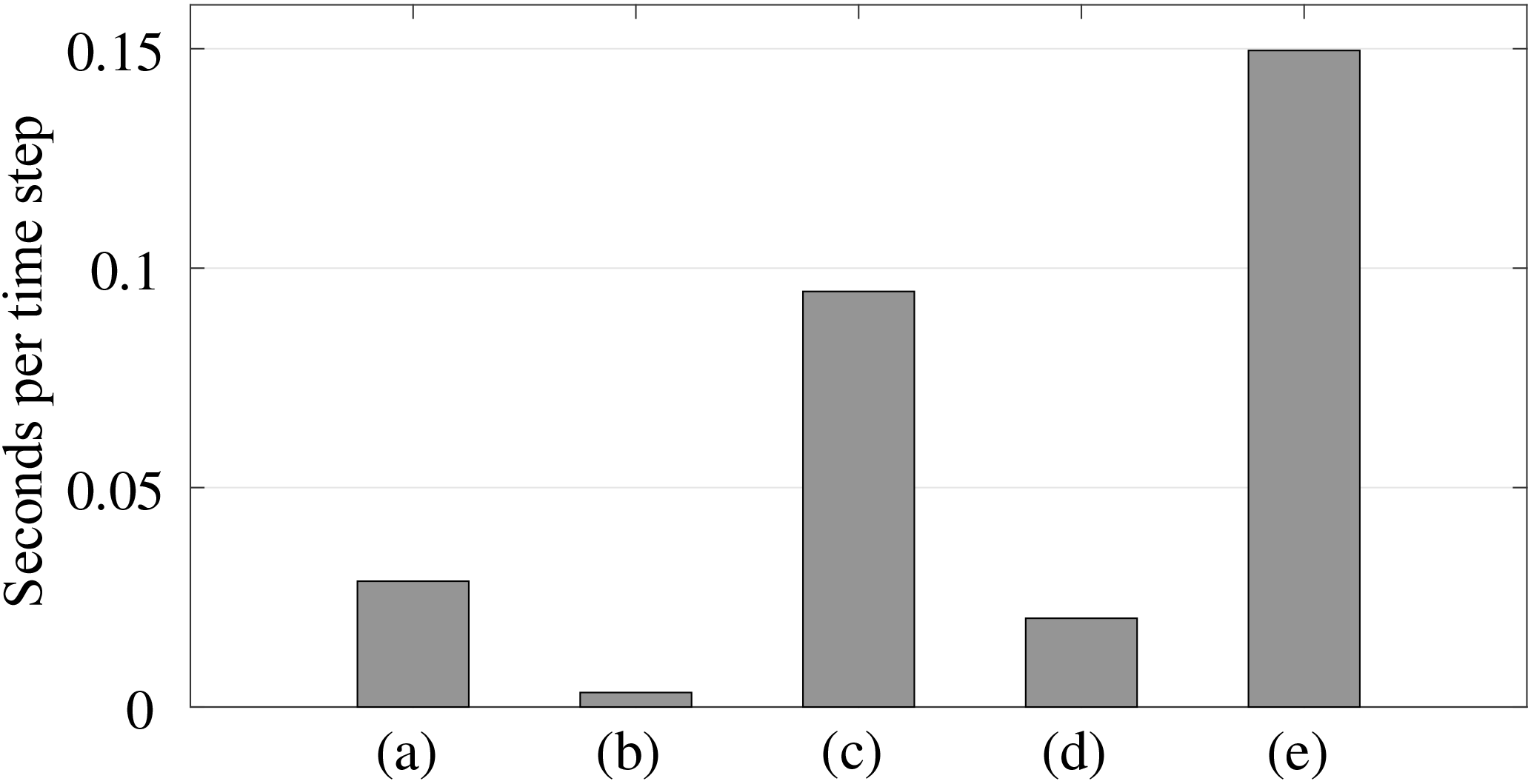
Figure 4Individual timing of the four modules of the time loop averaged over 10 k steps: (a) velocity gradient, (b) SGS, (c) convective term, (d) Poisson solver, and (e) total time loop. The numerical resolution is 1283, run with 64 MPI processes and a domain decomposition of 8×8.
3.4 Study cases
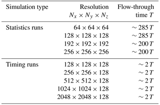
The goal of this study is to develop a cost–benefit analysis for the different, already established, dealiasing methods from a computational cost standpoint as well as in terms of accuracy in reproducing turbulent flow characteristics. For this reason, three different cases have been considered, corresponding to the three dealiasing methods considered: (a) the 3∕2 rule used as reference, (b) the FT method, and (c) the FS method. All the simulations have been run with a numerical resolution of , 1283, 1923, and 2563, with a domain size of , where zi is the height of the boundary layer taken here with a value of zi=1000 m. A uniform surface roughness of value is imposed, which is representative of sparse forest or farmland with many hedges (Brutsaert, 1982; Stull, 1988). The simulations have been initialized with a vertical logarithmic profile with added random noise for the component. The two other velocity components and have been initialized with an averaged zero velocity profile with added noise to generate the initial turbulence. The integration time step is set to Δt=0.2 s for the 643, 1283, and the 1923 simulations and to Δt=0.1 s for the 2563 simulation. These time steps ensure that stability requirements for the time integration scheme are met. The Smagorinsky constant and the wall damping exponent are set to CS=0.1 and n=2 (Mason, 1994; Porté-Agel et al., 2000; Sagaut, 2006).
For each dealiasing method, the simulations at 643, 1283, 1923, and 2562 were run until the flow reached statistic convergence of the friction velocity u* and the mean kinetic energy. This warm-up time was fixed to ∼95 T (where T is the flow-through time, defined as ). At this point, running averages were computed to evaluate the different flow statistics presented in the following sections. To provide long enough averaging times, the 643 and 1283 simulations were run for an additional ∼190 T. The 1923 and 2563 simulations were run for an additional ∼100 T. In parallel, runs with higher horizontal resolution were used to evaluate the computational cost of the dealiasing methods with increasing numerical resolution (timing runs). These last simulations were only run for a few thousand iterations. Table 1 contains a summary of all the simulations performed in this work.
Table 1Simulations summary, each simulation was run with the three different dealiasing methods.
4.1 Computational cost
The computational cost of evaluating the convective term, dealiased via the 3∕2 rule, the FT, and the FS is intercompared in Fig. 5. The horizontal resolution has been increased from 128×128 to 2048×2048 collocation nodes to highlight how the different methods scale. Only the horizontal resolution is changed given that the vertical direction is treated in physical space with the second-order accurately centered finite-difference method. Note that such a method does not typically require any dealiasing treatment, because the truncation error tends to decrease the aliasing errors (Canuto et al., 2006; Kravchenko et al., 1996). In Fig. 5, the ordinate axis is divided by nx⋅ny to show the effect of the increase in resolution on the computational cost. The number of MPI processes and the domain decomposition have been kept identical to avoid introducing effects from the parallelization scaling into the results. Hence, only the effect of the resolution change on the computation time of the dealiasing methods is presented here. Results confirm that the computational cost of the convective term is notably smaller when using the FT and FS dealiasing methods, with gains of 30 % at and 23 % at . The results follow the computational cost calculated by the number of operations presented in Sect. 2, which predicted a gain of up to 35% for runs with 40963 grid nodes. The deviation in the computational cost present in Fig. 5 is the result of the varying load of the computer cluster since all simulations were run using the same number of nodes to avoid having to add the code's scaling properties to the analysis. From the results it is also important to note that there is no significant difference in the computational cost between the FT and FS methods, given that both use the same grid size and hence the corresponding numerical complexity of both methods is similar. It is also worth mentioning that these methods are simpler to implement and require less rapid-access memory when compared to the 3∕2 rule, as there is no need to extend either the numerical grid or the wavenumber range.
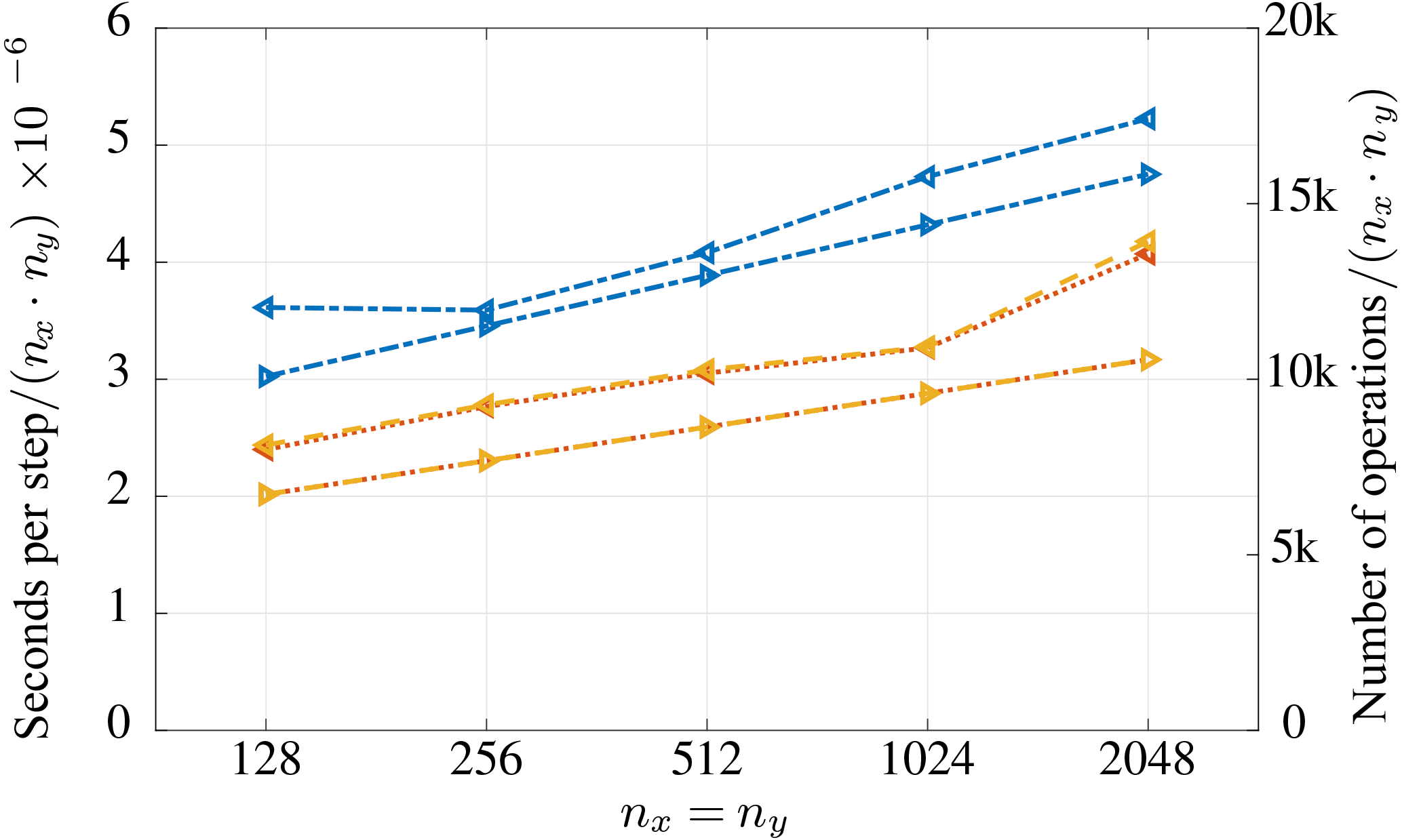
Figure 5Computational cost of the convective module as a function of the horizontal resolution. The timing of the module is presented on the left vertical axis and represented by left-pointing arrows. The number of operations is shown on the right vertical axis and represented by right-pointing arrows. The three different dealiasing methods are plotted: the 3∕2 rule as the blue dot–dashed line, the FT method as the orange dotted line, and the FS method as the yellow dashed line. The numerical resolutions are , run with 64 MPI processes and a domain decomposition of 8×8 elements.
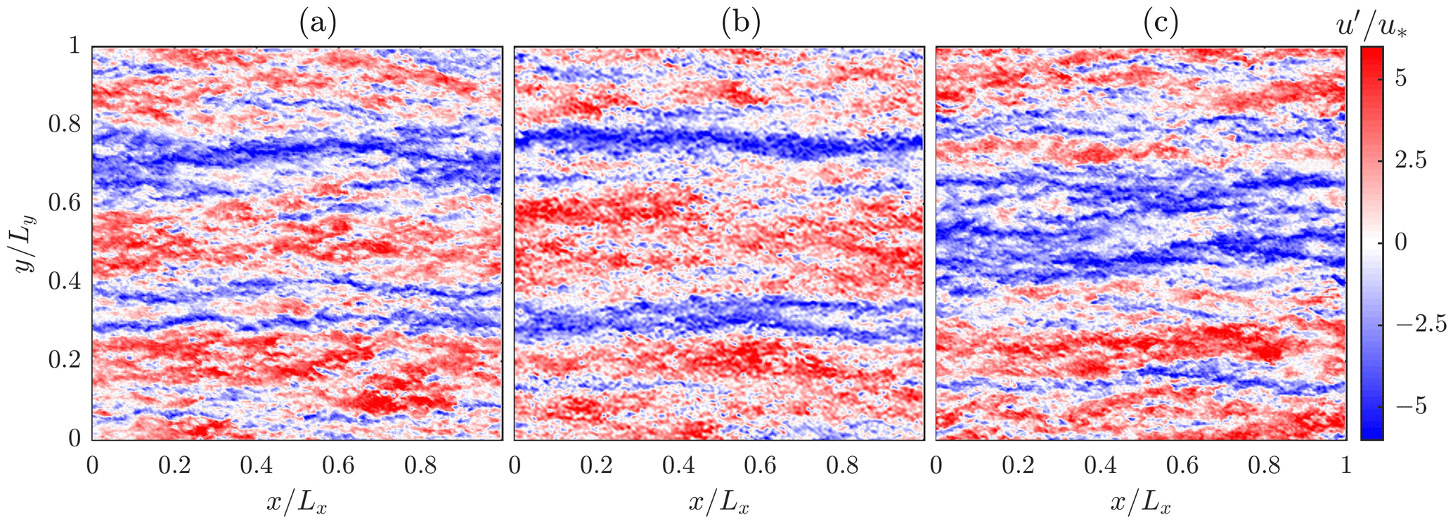
Figure 6Instantaneous streamwise velocity perturbation at for the three different dealiasing methods: (a) 3∕2 rule, (b) FT method, and (c) FS method. The numerical resolution is 2563.
In the following subsections, we compare the impact of the different dealiasing schemes on flow statistics. Profiles from runs using the 3∕2 rule for dealiasing will be taken as reference, and comments will focus on departures from such “exact” profiles when the FT or FS treatments are considered.
4.2 Flow statistics
Traditional flow metrics are investigated next and compared between the different dealiasing schemes. Results for the 1283, 1923, and 2563 cases are presented in this section. The results are normalized using the traditional scaling variables: the friction velocity (u*) and the boundary-layer height (zi). As a starting point, Fig. 6 shows an instantaneous snapshot (pseudo-color plots) of the streamwise velocity perturbation for the three dealiasing methods. An additional case without dealiasing in the convective term was run and resulted in a complete laminarization of the turbulent flow (not shown here), highlighting the importance of the dealiasing operation (Kravchenko and Moin, 1997). By contrast, when dealiasing schemes are applied, the instantaneous flow field appears qualitatively similar among the different cases. Irrespective of the dealiasing method that is used, streamwise elongated high- and low-momentum bulges flank each other, as is apparent in Fig. 6. This is a common phenomena in pressure-driven boundary-layer flows (Munters et al., 2016). Qualitatively, small differences can be appreciated on the structure and distribution of the smaller-scale turbulence within the flow only in the FT method. For example, the flow in panel b shows the effect of the cutoff filter, where high-frequency perturbations occur throughout the considered pseudo-color plot. These spurious oscillations have an impact on the flow statistics, as will be shown in the following.
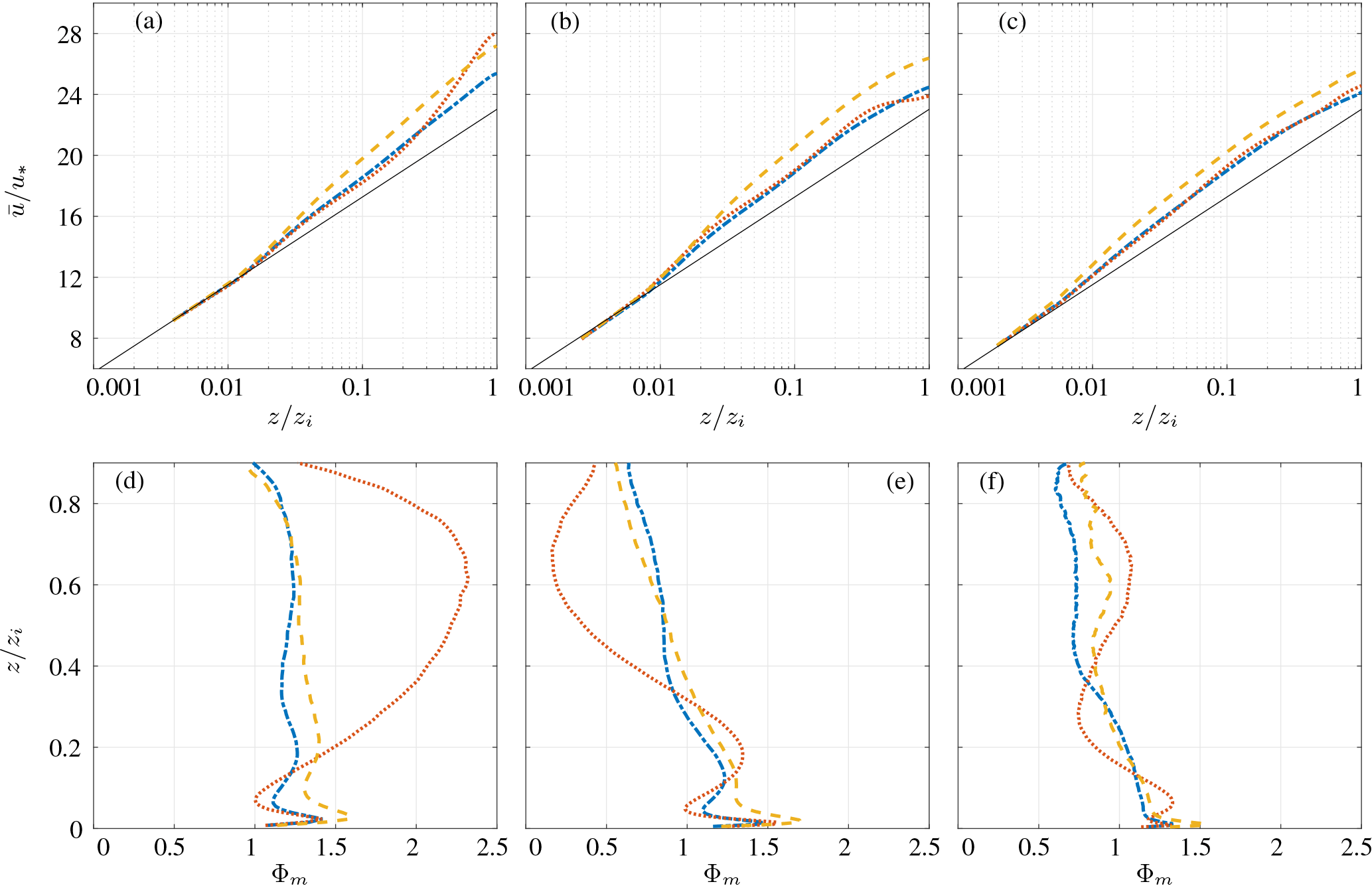
Figure 7Top panels represent the plots of the non-dimensional mean streamwise velocity profile for (a) the 1283 case, (b) the 1923 case, and (c) the 2563 case. Bottom panels represent the mean streamwise velocity gradient for (d) the 1283 case, (e) the 1923 case, and (f) the 2563 case. The lines represent the three different dealiasing methods: the 3∕2 rule as the blue dot–dashed line, the FT method as the red dotted line, and the FS method as the yellow dashed line. The solid line represents the ideal log–law profile.
The horizontally and temporally averaged velocity profiles are characterized by an approximately logarithmic behavior within the surface layer (z≈0.15zi, as is apparent from Fig. 7, where results are illustrated for the following three resolutions: 1283, 1923, and 2563). For the 1283 case, the observed departure from the logarithmic profile for the 3∕2-rule case is in excellent agreement with results from previous literature for this particular SGS model (Bou-Zeid et al., 2005; Porté-Agel et al., 2000). When using the FT method, the agreement of the averaged velocity profile with the corresponding 3∕2-rule profiles improves with increasing resolution. While in the 1283 case a good estimation of the logarithmic flow is obtained at the surface layer, there is a large acceleration of the flow further above. This overshoot does not occur for the higher-resolution runs. When using the FS method, the mean velocity magnitude is consistently overpredicted throughout the domain, and the situation does not improve with increasing resolution (the overshoot is up to 7.5 % for the 1283, 8.5 % for the 1923, and 7 % for the 2563 run). Further comparing the results obtained by the FS and FT methods with those obtained with the 3∕2 rule, it is clear that while the FS method presents a generalized overestimation of the velocity with an overall good logarithmic trend, the FT method presents a better adjustment in the surface layer with larger departures from the logarithmic regime in the upper-domain region that decrease with increasing numerical resolution. The mean kinetic energy of the system is overestimated by and by the FT and FS methods, when compared to that of runs using the 3∕2 rule in the 2563 case. Overall, the mean kinetic energy is larger for the FT and FS cases, when compared to the 3∕2-rule case, even at the highest of the considered resolutions ( and by the FT and FS methods for the 2563 case). Such behavior can be related to the low-pass filtering operation that is performed in the near-wall regions, which tends to reduce resolved turbulent stresses in the near-wall region, resulting in a higher mass flux for the considered flow system. This is more apparent for the low-resolution cases.
Mean velocity gradient profiles () are also featured in Fig. 7d, e, and f. Profiles at each of the considered resolutions present a large overshoot near the surface, which is a well-known problem in LES of wall-bounded flows and has been extensively discussed in the literature (Bou-Zeid et al., 2005; Brasseur and Wei, 2010; Lu and Porté-Agel, 2013). In comparing the results between the FS and FT method with the 3∕2 rule, it can be observed that there are stronger gradients in the mean velocity profile within the surface layer when using the FS method. This leads to the observed shift in the mean velocity profile. Conversely, when using the FT method, departures are of an oscillatory nature, leading to less pronounced variations in the mean velocity profile when compared to the reference ones (the 3∕2-rule cases). This behavior is consistently found across the considered resolutions, but the situation ameliorates as resolution is increased (i.e., weaker departures).
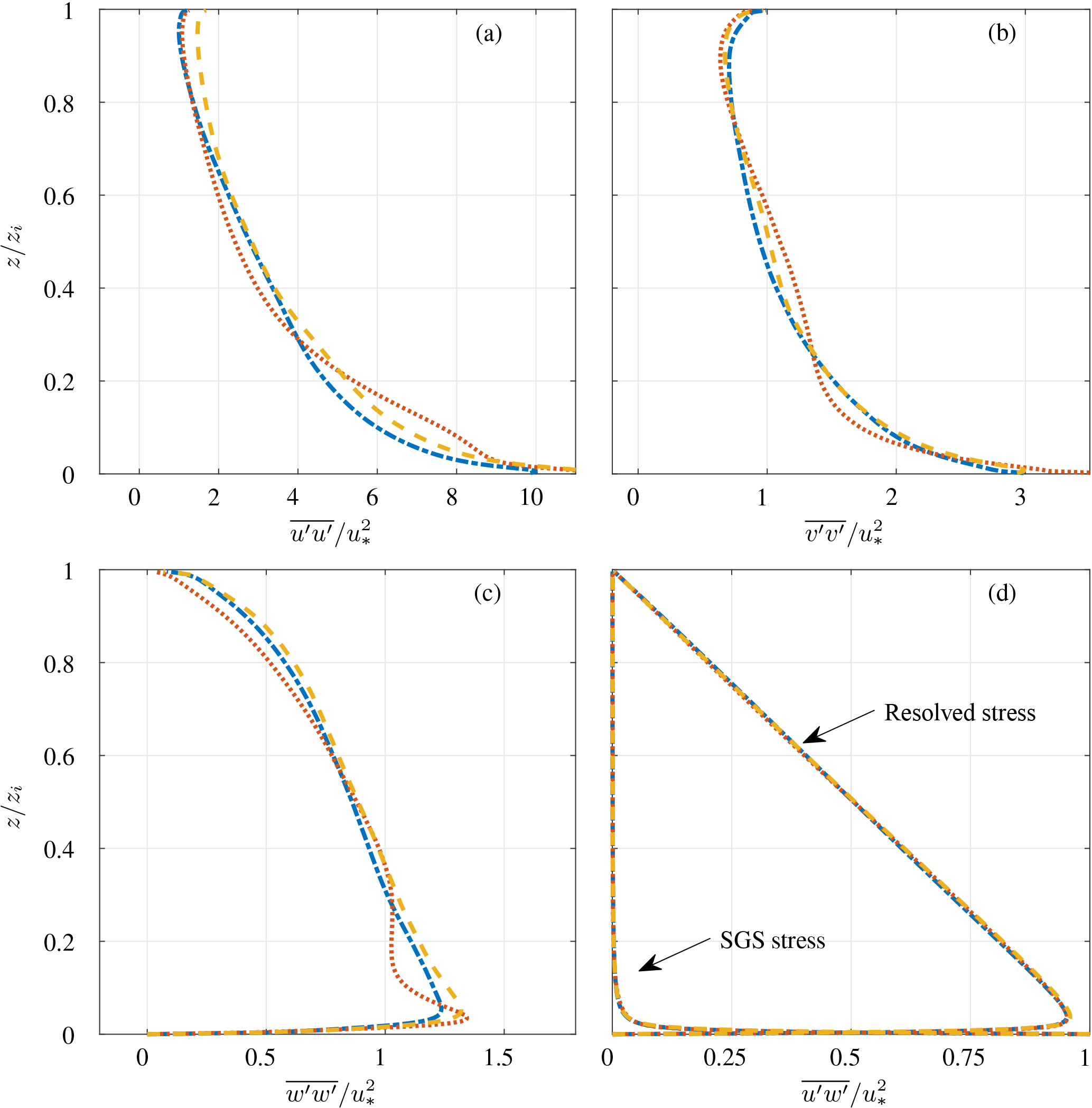
Figure 8Profiles of the non-dimensional variances (a–c) and shear stress (d) using a numerical resolution of 2563 for the three different dealiasing methods: the 3∕2 rule as the blue dot–dashed line, the FT method as the red dotted line, and the FS method as the yellow dashed line.
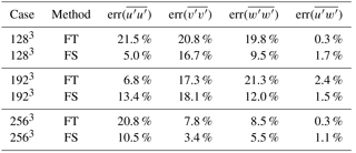
Figure 8 features the vertical structure of second-order statistics predicted via the FS and the FT methods, including a comparison with the corresponding predictions from the 3∕2-rule, 2563-study case. Note that when averaging in space and (subsequently) in time, the resulting profiles are comparable to those found in previously published LES studies (Bou-Zeid et al., 2005; Porté-Agel et al., 2000). The fact that the shear stress profiles are similar among the different dealiasing cases is also indicative of the fact that the SGS fraction is not strongly affected by the choice of dealiasing method, which is also partly due to the simplicity of the static Smagorinsky model that is being used. The potential effect that the different dealiasing schemes could have in more advanced subgrid models is discussed later on. Specifically, the error in the Reynolds shear stress (e.g., not including the SGS contribution) in the surface layer decreases with increasing resolution for the FS method (from 1.7 to 1.1 % for the 1283 and 2563, respectively) as indicated in Table 2 and also fluctuates around very small values for the FT method. When considering the diagonal stress tensor components across simulations, it is noteworthy that all such quantities are overpredicted when using the FT and the FS methods in the near-surface region (z⪅0.1). Further above, the FS method tends to consistently overpredict, whereas the FT method presents an oscillatory nature. As can be observed in Table 2, the mean error deviations decrease with increasing resolution for all cases, except for the streamwise variance where there is no clear trend.
Table 2Mean error in the variance profiles between the FT∕FS methods and the 3∕2 rule over the lower 15 % of the domain. For example, the error of the streamwise variance is computed as for .
To complement the analysis of the effect of the different dealiasing methods on the physical structure of the flow, the corresponding power spectra are investigated. According to Kolmogorov's energy cascade theory, the inertial subrange of the power spectrum should be characterized by a power law of slope (Kolmogorov, 1968). In this range the effects of viscosity, boundary conditions, and large-scale structures are not important. Also, in wall-bounded flows without buoyancy effects, a production range should also be present, following a power-law scaling of −1 (Calaf et al., 2013; Gioia et al., 2010; Katul et al., 2012). Figure 9 shows the energy spectra of the streamwise velocity obtained using the different dealiasing methods. The spectrum obtained using the 3∕2 rule matches well the traditional turbulent spectra presented in the literature (Bou-Zeid et al., 2005; Cerutti, 2000) and it is used to assess the effects introduced by the FT and FS dealiasing methods. From this spectral analysis, it can be observed that the high-wavenumber ranges are modified by both methods. The FT method sharply cuts the spectra at the scale of close to the LES filter-scale Δ. On the other hand, the FS method smoothly attenuates the effects of the aliasing errors at the high end of the spectra. The dealiasing methods have been designed for such behavior, since only the higher frequencies are filtered. From the FT method flow field spectra, the effect of the cutoff applied within the dealiasing scheme is clearly visible. It is apparent that the capacity of the LES solver to reproduce the fine-scale turbulence structure of the flow is strongly jeopardized when using the FT method and limited at the scale of close to the LES filter-scale Δ. Essentially, this method artificially over-dissipates the turbulent kinetic energy and yields to an overestimation of the mean kinetic energy. In contrast, the energy spectrum obtained using the FS method does not produce such a large energy cutoff. Therefore, a larger range of the spectrum is resolved and less turbulent kinetic energy is dissipated by aliasing errors.
Although the effect of the FT and FS methods on the small scale can be clearly observed in Fig. 9, their effect on the large scales also needs to be quantified. To compute a direct comparison scale by scale, the following ratio was used (Eq. 16) for the 1283, 1923, and 2563 simulations:
where Eu,k denotes the power spectral density of the u velocity component at wavenumber k and XX stands for the dealiasing method FT or FS. If ρ(k)<0, the energy density at that given wavenumber (k) is less than the corresponding one for the run using the 3∕2 rule; vice versa if ρ(k)>0. Figure 10 presents the ratio ρ(k) for both methods.
When using the FT method, energy at the low wavenumbers is underpredicted, whereas energy at the large wavenumbers is overpredicted. Departures are in general larger with decreasing resolution, with an excess of up to 100% for the 1283 simulations in the wavenumber range close to the cutoff wavenumber. By contrast, when using the FS method, the energy from the filtered (dealiased) small scales is redistributed quasi-uniformly throughout the spectra with an averaged overall variation of less than 13 %.
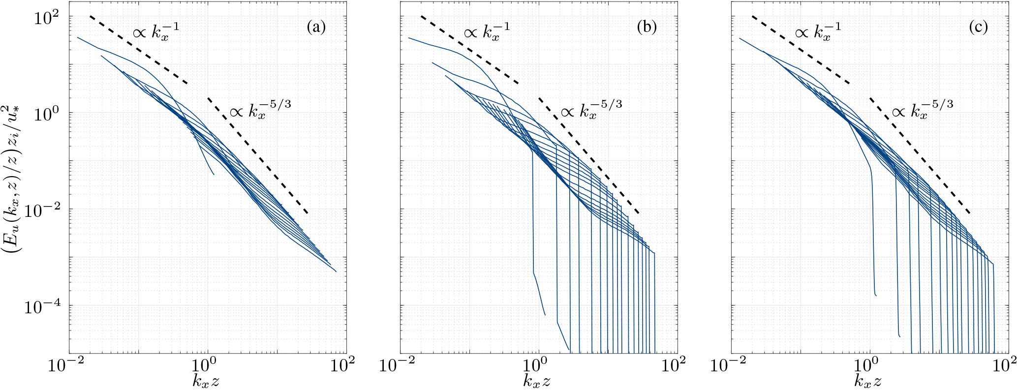
Figure 9Normalized streamwise spectra of the streamwise velocity as a function of kxz for the 1923 simulations. The three different dealiasing methods are the 3∕2 rule (a), the FT method (b), and the FS method (c) at heights , 0.0273, 0.0586, 0.0898, 0.1523, 0.2148, 0.3086, 0.4336, 0.5586, and 0.6211.
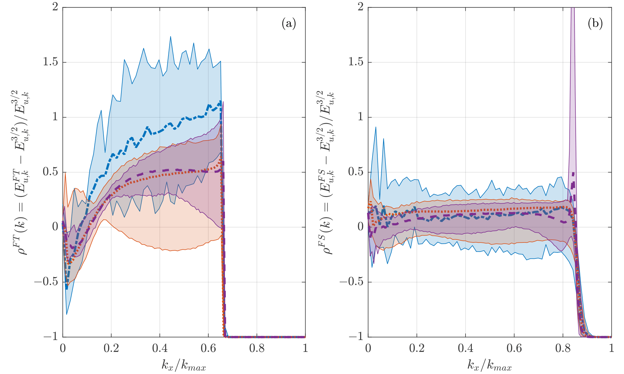
Figure 10Effect of the FT (a) and the FS (b) methods of the streamwise spectra of the streamwise velocity compare to the 3∕2 rule. The solid line represent the average value and the shaded area represent the extreme values. The resolutions are 1283 as the blue dot–dashed line, 1923 as the red dotted line, and 2563 as the purple dashed line.
In the development of this paper, focus has been directed to the study of the advantages and disadvantages of different dealiasing methods. In this regard, throughout the analysis, we have tried to keep the structure of the LES configuration as simple and canonical as possible to remove the effect of other add-on complexities. Additional complications might arise when considering additional physics; here we discuss the potential effect that these different dealiasing methods could have on them. One such element of added complexity is, for example, the use of more sophisticated subgrid-scale models based on dynamic approaches to determine the values of the Smagorinsky constant (Bou-Zeid et al., 2005; Germano et al., 1991). In most of these advanced subgrid models, information from the small-scale turbulent eddies is used to determine the evolution of the subgrid constant. However, in both the FT and FS method, the small turbulent scales are severely affected, and hence the use of dynamic subgrid models could be severely hampered unless these are accordingly modified and adjusted, for example via filtering at larger scales than the usual grid scale. Another element of added complexity consists of using more realistic atmospheric forcing, considering for example the effect of the Coriolis force with flow rotation as a function of height and velocity magnitude. In this case, we hypothesize that the FT method could lead to stronger influences on the resultant flow field as this dealiasing technique not only affects the distribution of energy on small turbulent scales but also on large scales (as is apparent from Fig. 10), the latter being potentially more affected by the Coriolis force. This represents a strong nonlinear effect that is hard to quantify, and hence further testing, including realistic forcing with a geostrophic wind and Coriolis force, would be required to better quantify these effects. Also, often in LES studies of atmospheric flows, one is interested in including an accurate representation of scalar transport (passive/active). In this case the differential equations do not include a pressure term, and hence most of the computational cost is linked to the evaluation of the convective term. As a result, the benefit of using alternative, cheaper dealiasing techniques (FT or FS) will be even more advantageous, yet the total gain is not trivial to evaluate a priori, and the effect on the scalar fields should also be further evaluated.
In general, we believe that it is not fair to advocate for one or other dealiasing method based on the results of this analysis. Note that the goal of this work is to provide an objective analysis of the advantages and limitations that the different methods provide, leaving the readers with the ultimate responsibility of choosing the option that will adjust better to their application. For example, while having exact dealiasing (3∕2 rule) might be better in studies focusing on turbulence and dispersion, one might be better off using a simpler and faster dealiasing scheme to run the traditionally expensive warm-up runs or to evaluate surface drag in flow over urban and vegetation canopies, where most of the surface force is due to pressure differences (Patton et al., 2016).
The Fourier-based pseudo-spectral collocation method (Canuto et al., 2006; Orszag, 1970; Orszag and Pao, 1975) remains the preferred workhorse in simulations of wall-bounded flows over horizontally periodic regular domains and is often used in conjunction with a centered finite-difference or Chebychev polynomial expansions in the vertical direction (Kopriva and Kolia, 1996; Moeng and Sullivan, 2015; Shah and Bou-Zeid, 2014). This approach is often used because of the high-order accuracy and the intrinsic efficiency of the fast Fourier transform algorithm (Cooley and Tukey, 1965; Frigo and Johnson, 2005). In this technique, aliasing that arises when evaluating the quadratic nonlinear term in the NS equations can severely deteriorate the quality of the solution and hence needs to be treated adequately. In this work, a performance–cost analysis has been developed for three well-accepted dealiasing techniques – the 3∕2 rule, the FT method and the FS method – to evaluate the corresponding advantages and limitations. The 3∕2 rule requires a computationally expensive padding and truncation operation, while the FT and FS methods provide an approximate dealiasing by low-pass filtering the signal over the available wavenumbers, which comes at a reduced cost.
The presented results show compelling evidence of the benefits of these methods as well as some of their drawbacks. The advantage of using the FT or the FS approximate dealiasing methods is their reduced computational cost (cutback on the total simulation time of ∼15 % for the 1283 case, ∼21 % for the 2563 case), with an increased gain as the numerical resolution is increased. Regarding the flow statistics, results illustrate that both the FT and the FS methods yield less accurate results when compared to those obtained with the traditional 3∕2 rule, as one could expect.
Specifically, results illustrate that both the FT and FS methods over-dissipate the turbulent motions in the near-wall region, yielding an overall higher mass flux when compared to the reference one (3∕2 rule). Regarding the variances, results illustrate modest errors in the surface layer, with local departures in general below 10 % of the reference value across the considered resolutions. The observed departures in terms of mass flux and velocity variances tend to reduce with increasing resolution. Analysis of the streamwise velocity spectra has also shown that the FT method redistributes unevenly the energy across the available wavenumbers, leading to an overestimation of the energy of some scales by up to 100 %. By contrast, the FS method redistributes the energy evenly, yielding a modest +13 % energy magnitude throughout the available wavenumbers. Compared to the 3∕2 rule, these differences in flow statistics are the result of the sharp low-pass filter applied in the FT method and the smooth filter that characterizes the FS method.
The sources of the LES code developed at the University of Utah are accessible in prerelease at https://doi.org/10.5281/zenodo.1048338 (Margairaz et al., 2017).
Due to the large amount of data generated during this study, no lasting structure can be permanently supported where to freely access the data. However, access can be provided using the Temporary Guest Transfer Service of the Center of High Performance Computing of the University of Utah. To get access to the data, Marc Calaf (marc.calaf@utah.edu) will provide temporary login information for the sftp server.
The authors declare no competing interests
Fabien Margairaz and Marc Calaf acknowledge the Mechanical Engineering
Department at the University of Utah for start-up funds. Marco G. Giometto
acknowledges the Civil Engineering and Engineering Mechanics Department at
Columbia University for start-up funds. Marc B. Parlange is grateful to NSERC
and Monash University for their support. The authors would also like to
recognize the computational support provided by the Center for High
Performance Computing (CHPC) at the University of Utah as well as the Extreme
Science and Engineering Discovery Environment (XSEDE) platform (project
TG-ATM170018).
Edited by: Simone
Marras
Reviewed by: Elie Bou-Zeid and one anonymous referee
Abkar, M. and Porté-Agel, F.: Mean and turbulent kinetic energy budgets inside and above very large wind farms under conventionally-neutral condition, Renew. Energ., 70, 142–152, https://doi.org/10.1016/j.renene.2014.03.050, 2014. a
Albertson, J. D.: Large Eddy Simulation of Land-Atmosphere Interaction, Ph.D. thesis, University of California at Davis, Hydrol. Sci., an optional note, 1996. a
Albertson, J. D. and Parlange, M. B.: Natural integration of scalar fluxes from complex terrain, Adv. Water Resour., 23, 239–252, https://doi.org/10.1016/S0309-1708(99)00011-1, 1999. a, b
Albertson, J. D., Parlange, M. B., Katul, G. G., Chu, C.- R., Stricker, H., and Tyler, S.: Sensible Heat Flux From Arid Regions: A Simple Flux-Variance Method, Water Resour. Res., 31, 969973, https://doi.org/10.1029/94WR02978, 1995. a
Allaerts, D. and Meyers, J.: Boundary-layer development and gravity waves in conventionally neutral wind farms, J. Fluid Mechan., 814, 95–130, https://doi.org/10.1017/jfm.2017.11, 2017. a
Anderson, W., Passalacqua, P., Porté-Agel, F., and Meneveau, C.: Large-Eddy Simulation of Atmospheric Boundary-Layer Flow Over Fluvial-Like Landscapes Using a Dynamic Roughness Model, Bound.-Lay. Meteorol., 144, 263–286, https://doi.org/10.1007/s10546-012-9722-9, 2012. a
Bernaschi, M., Fatica, M., Melchionna, S., Succi, S., and Kaxiras, E.: A flexible high-performance Lattice Boltzmann GPU code for the simulations of fluid flows in complex geometries, Concurr. Comput. Pract. Exper., 22, 1–14, https://doi.org/10.1002/cpe.1466, 2010. a, b
Bou-Zeid, E.: Challenging the large eddy simulation technique with advanced a posteriori tests, J. Fluid Mechan., 764, 1–4, https://doi.org/10.1017/jfm.2014.616, 2014. a
Bou-Zeid, E., Meneveau, C., and Parlange, M. B.: Large-eddy simulation of neutral atmospheric boundary layer flow over heterogeneous surfaces: Blending height and effective surface roughness, Water Resour. Res., 40, W02505, https://doi.org/10.1029/2003WR002475, 2004. a
Bou-Zeid, E., Meneveau, C., and Parlange, M. B.: A scale-dependent Lagrangian dynamic model for large eddy simulation of complex turbulent flows, Phys. Fluids, 17, 025105, https://doi.org/10.1063/1.1839152, 2005. a, b, c, d, e, f
Bowman, J. C. and Roberts, M.: Efficient Dealiased Convolutions without Padding, SIAM J. Sci. Comput., 33, 386–406, https://doi.org/10.1137/100787933, 2011. a
Brasseur, J. G. and Wei, T.: Designing large-eddy simulation of the turbulent boundary layer to capture law-of-the-wall scaling, Phys. Fluids, 22, 1–21, https://doi.org/10.1063/1.3319073, 2010. a, b
Brutsaert, W.: Evaporation into the Atmosphere, Springer Netherlands, Dordrecht, https://doi.org/10.1007/978-94-017-1497-6, 1982. a
Burkardt, J., Gunzburger, M., and Lee, H.-C.: POD and CVT-based reduced-order modeling of Navier–Stokes flows, Comput. Method. Appl. Mechan. Eng., 196, 337–355, https://doi.org/10.1016/j.cma.2006.04.004, 2006. a
Calaf, M., Meneveau, C., and Meyers, J.: Large eddy simulation study of fully developed wind-turbine array boundary layers, Phys. Fluids (1994–present), 22, 015110, https://doi.org/10.1063/1.3291077, 2010. a
Calaf, M., Meneveau, C., and Parlange, M. B.: Direct and Large-Eddy Simulation VIII, in: ERCOFTAC Series, Vol. 15, Springer Netherlands, Dordrecht, https://doi.org/10.1007/978-94-007-2482-2, 2011. a
Calaf, M., Hultmark, M., Oldroyd, H. J., Simeonov, V., and Parlange, M. B.: Coherent structures and the k-1 spectral behaviour, Phys. Fluids, 25, 125107, https://doi.org/10.1063/1.4834436, 2013. a
Canuto, C., Hussaini, M. Y., Quarteroni, A., and Zang, T. A.: Spectral Methods: Fundamentals in Single Domain, Springer-Verlag, Berlin, 2006. a, b, c, d, e, f, g, h, i
Canuto, C., Hussaini, M. Y., Quarteroni, A., and Zang, T. A.: Spectral Methods: Evolution to Complex Geometries and Applications to Fluid Dynamics, Springer-Verlag, Berlin, 2007. a
Cassiani, M., Katul, G. G., and Albertson, J. D.: The Effects of Canopy Leaf Area Index on Airflow Across Forest Edges: Large-eddy Simulation and Analytical Results, Bound.-Lay. Meteorol., 126, 433–460, https://doi.org/10.1007/s10546-007-9242-1, 2008. a
Cerutti, S.: Spectral and hyper eddy viscosity in high-Reynolds-number turbulence, J. Fluid Mechan., 421, 307–338, 2000. a
Chorin, A. J.: The numerical solution of the Navier-Stokes equations for an incompressible fluid, B. Am. Mathe. Soc., 73, 928–932, https://doi.org/10.1090/S0002-9904-1967-11853-6, 1967. a
Chorin, A. J.: Numerical solution of the Navier-Stokes equations, Math. Comput., 22, 745–762, https://doi.org/10.2307/2004575, 1968. a
Cooley, J. W. and Tukey, J. W.: An algorithm for the machine calculation of complex Fourier series, Mathe. Comput., 19, 297–297, https://doi.org/10.1090/S0025-5718-1965-0178586-1, 1965. a, b
Frigo, M. and Johnson, S. G.: The design and implementation of FFTW3, Proc. IEEE, 93, 216–231, https://doi.org/10.1109/JPROC.2004.840301, 2005. a, b
Germano, M., Piomelli, U., Moin, P., and Cabot, W. H.: A dynamic subgrid-scale eddy viscosity model, Phys. Fluids A, 3, 1760–1765, https://doi.org/10.1063/1.857955, 1991. a, b
Gioia, G., Guttenberg, N., Goldenfeld, N., and Chakraborty, P.: Spectral Theory of the Turbulent Mean-Velocity Profile, Phys. Rev. Lett., 105, 184501, https://doi.org/10.1103/PhysRevLett.105.184501, 2010. a
Giometto, M. G., Christen, A., Meneveau, C., Fang, J., Krafczyk, M., and Parlange, M. B.: Spatial Characteristics of Roughness Sublayer Mean Flow and Turbulence Over a Realistic Urban Surface, Bound.-Lay. Meteorol., 160, 425452, https://doi.org/10.1007/s10546-016-0157-6, 2016. a
Giometto, M. G., Christen, A., Egli, P., Schmid, M. F., Tooke, R. T., Coops, N. C., and Parlange, M. B.: Effects of trees on mean wind, turbulence and momentum exchange within and above a real urban environment, Adv. Water Resour., 106, 154–168, https://doi.org/10.1016/j.advwatres.2017.06.018, 2017. a
Hamada, T., Narumi, T., Yokota, R., Yasuoka, K., Nitadori, K., and Taiji, M.: 42 TFlops hierarchical N -body simulations on GPUs with applications in both astrophysics and turbulence, in: Proceedings of the Conference on High Performance Computing Networking, Storage and Analysis – SC '09, p. 1, ACM Press, New York, New York, USA, https://doi.org/10.1145/1654059.1654123, 2009. a
Horiuti, K.: Comparison of conservative and rotational forms in large eddy simulation of turbulent channel flow, J. Computat. Phys., 71, 343–370, https://doi.org/10.1016/0021-9991(87)90035-0, 1987. a
Hou, T. Y. and Li, R.: Computing nearly singular solutions using pseudo-spectral methods, J. Comput. Phys., 226, 379–397, https://doi.org/10.1016/j.jcp.2007.04.014, 2007. a, b, c, d
Hsu, M. C., Akkerman, I., and Bazilevs, Y.: High-performance computing of wind turbine aerodynamics using isogeometric analysis, Comput. Fluids, 49, 93–100, https://doi.org/10.1016/j.compfluid.2011.05.002, 2011. a
Hughes, T. J. R., Cottrell, J. A., and Bazilevs, Y.: Isogeometric analysis: CAD, finite elements, NURBS, exact geometry and mesh refinement, Comput. Methods Appl. Mechan. Eng., 194, 4135–4195, https://doi.org/10.1016/j.cma.2004.10.008, 2005. a
Hultmark, M., Vallikivi, M., Bailey, S. C. C., and Smits, A. J.: Logarithmic scaling of turbulence in smooth- and rough-wall pipe flow, J. Fluid Mechan., 728, 376–395, https://doi.org/10.1017/jfm.2013.255, 2013. a
Iovieno, M., Cavazzoni, C., and Tordella, D.: A new technique for a parallel dealiased pseudospectral Navier-Stokes code, Comput. Phys. Commun., 141, 365–374, https://doi.org/10.1016/S0010-4655(01)00433-7, 2001. a
Kármán, T. V.: Mechanical similitude and turbulence, Nachrichten von der Gesellschaft der Wissenschaften zu Gottingen – Fachgruppe I (Mathematik), 5, 1–19, 1931. a
Katul, G. G., Porporato, A., and Nikora, V.: Existence of k-1 power-law scaling in the equilibrium regions of wall-bounded turbulence explained by Heisenberg's eddy viscosity, Phys. Rev. E, 86, 066311, https://doi.org/10.1103/PhysRevE.86.066311, 2012. a
Kolmogorov, A.: Local structure of turbulence in an incompressible viscous fluid at very high Reynolds numbers, Phys.-Uspekhi, 734, 1–4, 1968. a, b
Kopriva, D. A. and Kolias, J. H.: A Conservative Staggered-Grid Chebyshev Multidomain Method for Compressible Flows, J. Comput. Phys., 125, 244–261, https://doi.org/10.1006/jcph.1996.0091, 1996. a
Kravchenko, A. and Moin, P.: On the Effect of Numerical Errors in Large Eddy Simulations of Turbulent Flows, J. Computat. Phys., 131, 310–322, https://doi.org/10.1006/jcph.1996.5597, 1997. a, b, c
Kravchenko, A. A., Moin, P., and Moser, R. D.: Zonal embedded grids for numerical simulations of wall-bounded turbulent flows, J. Comput. Phys., 423, 412–423, https://doi.org/10.1006/jcph.1996.0184, 1996. a
Lesieur, M. and Metais, O.: New Trends in Large-Eddy Simulations of Turbulence, Annual Review of Fluid Mechanics, 28, 45–82, https://doi.org/10.1146/annurev.fl.28.010196.000401, 1996. a
Li, N. and Laizet, S.: 2DECOMP & FFT-A Highly Scalable 2D Decomposition Library and FFT Interface, Cray User Group 2010 conference, 1–13, 2010. a, b, c
Lilly, D.: Representation of small scale turbulence in numerical simulation experiments, Proceedings of the IBM Scientific Computing Symposium on Environmental Sciences, 195–210, https://doi.org/10.5065/D62R3PMM, 1967. a
Lu, H. and Porté-Agel, F.: A modulated gradient model for scalar transport in large-eddy simulation of the atmospheric boundary layer, Phys. Fluids, 25, 0–17, https://doi.org/10.1063/1.4774342, 2013. a
Lu, H. and Porté-Agel, F.: On the Development of a Dynamic Non-linear Closure for Large-Eddy Simulation of the Atmospheric Boundary Layer, Bound.-Lay. Meteorol., 151, 1–23, https://doi.org/10.1007/s10546-013-9906-y, 2014. a
Margairaz, F., Calaf, M., Giometto, M. G.: fmargairaz/LES-Utah: LES-Utah-momentum, Zenodo, https://doi.org/10.5281/zenodo.1048338, 2017. a, b
Mason, P. J.: Large-eddy simulation: A critical review of the technique, Q. J. Roy. Meteorol. Soc., 120, 1–26, https://doi.org/10.1002/qj.49712051503, 1994. a
Mason, P. J. and Thomson, D. J.:Stochastic backscatter in large-eddy simulations of boundary layers, J. Fluid Mechan., 242, 51–78 https://doi.org/10.1017/S0022112092002271, 1992. a
Meneveau, C., Lund, T. S., and Cabot, W. H.: A Lagrangian dynamic subgrid-scale model of turbulence, J. Fluid Mechan., 319, 353–385, https://doi.org/10.1017/S0022112096007379, 1996. a
Moeng, C. and Sullivan, P. P.: Large-Eddy Simulation, in: Encyclopedia of Atmospheric Sciences, 232–240, Elsevier, https://doi.org/10.1016/B978-0-12-382225-3.00201-2, 2015. a, b, c
Moeng, C.-H.: A large-eddy-simulation model for the study of planetary boundary-layer turbulence, J. Atmos. Sci., 41, 2052–2062, https://doi.org/10.1175/1520-0469(1984)041<2052:ALESMF>2.0.CO;2, 1984. a, b, c
Moeng, C.-H. and Wyngaard, J. C.: Spectral Analysis of Large-Eddy Simulations of the Convective Boundary Layer, J. Atmos. Sci., 45, 3573–3587, https://doi.org/10.1175/1520-0469(1988)045<3573:SAOLES>2.0.CO;2, 1988. a, b
Moin, P. and Kim, J.: Numerical investigation of turbulent channel flow, J. Fluid Mechan., 118, 341–377, https://doi.org/10.1017/S0022112082001116, 1982. a
Moore, G. E.: Cramming more components onto integrated circuits (Reprinted from Electronics, 114–117, 19 April 1965), Electronics, 38, 114–117, https://doi.org/10.1109/N-SSC.2006.4785860, 1965. a
Moser, R. D. R., Moin, P., and Leonard, A.: A spectral numerical method for the Navier-Stokes equations with applications to Taylor-Couette flow, J. Comput. Phys., 52, 524–544, https://doi.org/10.1016/0021-9991(83)90006-2, 1983. a, b
Munters, W., Meneveau, C., and Meyers, J.: Shifted periodic boundary conditions for simulations of wall-bounded turbulent flows, Phys. Fluids, 28, 025112, https://doi.org/10.1063/1.4941912, 2016. a
Najm, H. N.: Uncertainty Quantification and Polynomial Chaos Techniques in Computational Fluid Dynamics, Annu. Rev. Fluid Mechan., 41, 35–52, https://doi.org/10.1146/annurev.fluid.010908.165248, 2009. a
Orszag, S. A.: Analytical theories of turbulence, J. Fluid Mechan., 41, 363–386, https://doi.org/10.1017/S0022112070000642, 1970. a, b
Orszag, S. A.: On the Elimination of Aliasing in Finite-Difference Schemes by Filtering High-Wavenumber Components, J. Atmos. Sci., 1074–1074, https://doi.org/10.1175/1520-0469(1971)028<1074:oteoai>2.0.co;2, 1971. a, b, c
Orszag, S. A.: Comparison of Pseudospectral and Spectral Approximation, Stud. Appl. Mathe., 51, 253–259, https://doi.org/10.1002/sapm1972513253, 1972. a
Orszag, S. A. and Pao, Y.-H.: Numerical Computation of Turbulent Shear Flows, in: Turbulent Diffusion in Environmental Pollution, Proceedings of a Symposium held at Charlottesville, edited by: Frenkiel, F. N. and Munn, R. E., Vol. 18, Part A of Adv. Geophys., 225–236, Elsevier, https://doi.org/10.1016/S0065-2687(08)60463-X, 1975. a, b
Patterson, G. S.: Spectral Calculations of Isotropic Turbulence: Efficient Removal of Aliasing Interactions, Phys. Fluids, 14, 2538–2541, https://doi.org/10.1063/1.1693365, 1971. a, b, c
Patton, E. G., Sullivan. P. P., Shaw, R. H., Finnigan, J. J., and Weil, J. C.: Atmospheric Stability Influences on Coupled Boundary Layer and Canopy Turbulence, J. Atmos. Sci., 73, 1621–1647, https://doi.org/10.1175/JAS-D-15-0068.1, 2016 a
Piomelli, U.: Large-eddy simulation: achievements and challenges, Prog. Aerosp. Sci., 35, 335–362, https://doi.org/10.1016/S0376-0421(98)00014-1, 1999. a
Porté-Agel, F., Meneveau, C., and Parlange, M. B.: A scale-dependent dynamic model for large-eddy simulation: application to a neutral atmospheric boundary layer, J. Fluid Mechan., 415, 261–284, https://doi.org/10.1017/S0022112000008776, 2000. a, b, c, d
Prandtl, L.: Zur Turbulenten Strömung in Rohren und langs Glätten, Ergebnisse der Aerodynamischen Versuchsanstalt zu Göttingen, B. 4, 18–29, 1932. a
Sagaut, P.: Large Eddy Simuation of Incompressible Flow, Springer, 3rd Edn., 2006. a
Saiki, E. M., Moeng, C.-h., and Sullivan, P. P.: Large-Eddy Simulation of the stably stratified Planetary Boundary Layer, Bound.-Lay. Meteorol., 95, 1–30, https://doi.org/10.1023/A:1002428223156, 2000. a
Salesky, S. T., Chamecki, M., and Bou-Zeid, E.: On the Nature of the Transition Between Roll and Cellular Organization in the Convective Boundary Layer, Bound.-Lay. Meteorol., 163, 1–28, https://doi.org/10.1007/s10546-016-0220-3, 2016. a
Schlatter, P. and Örlü, R.: Turbulent boundary layers at moderate Reynolds numbers: inflow length and tripping effects, J. Fluid Mechan., 710, 5–34, https://doi.org/10.1017/jfm.2012.324, 2012. a
Shah, S. and Bou-Zeid, E.: Very-Large-Scale Motions in the Atmospheric Boundary Layer Educed by Snapshot Proper Orthogonal Decomposition, Bound.-Lay. Meteorol., 153, 355–387, https://doi.org/10.1007/s10546-014-9950-2, 2014. a
Skamarock, W., Klemp, J., Dudhi, J., Gill, D., Barker, D., Duda, M., Huang, X.-Y., Wang, W., and Powers, J.: A Description of the Advanced Research WRF Version 3, Technical Report, p. 113, https://doi.org/10.5065/D6DZ069T, 2008. a
Smagorinsky, J.: General circulation experiments with primirive equations, Mon. Weather Rev., 91, 99–164, https://doi.org/10.1175/1520-0493(1963)091<0099:GCEWTP>2.3.CO;2, 1963. a, b
Stoll, R. and Porté-Agel, F.: Large-eddy simulation of the stable atmospheric boundary layer using dynamic models with different averaging schemes, Bound.-Lay. Meteorol., 126, 1–28, https://doi.org/10.1007/s10546-007-9207-4, 2008. a
Stull, R. B.: An Introduction to Boundary Layer Meteorology, Springer Netherlands, Dordrecht, https://doi.org/10.1007/978-94-009-3027-8, 1988. a
Sullivan, P. P. and Patton, E. G.: The Effect of Mesh Resolution on Convective Boundary Layer Statistics and Structures Generated by Large-Eddy Simulation, J. Atmos. Sci., 68, 2395–2415, https://doi.org/10.1175/JAS-D-10-05010.1, 2011. a
Sullivan, P. P., McWilliams, J. C., and Moeng, C.-H.: A subgrid-scale model for large-eddy simulation of planetary boundary-layer flows, Bound.-Lay. Meteorol., 71, 247–276, https://doi.org/10.1007/BF00713741, 1994. a
Takahashi, D.: Forty years of Moore's Law, The Seattle Times, available at: https://www.seattletimes.com/business/forty-years-of-moores-law, 18 April 2005. a
Takizawa, K. and Tezduyar, T. E.: Multiscale space-time fluid-structure interaction techniques, in: Computational Mechanics, Springer-Verlag, Vol. 48, 247–267, https://doi.org/10.1007/s00466-011-0571-z, 2011. a
Voller, V. and Porté-Agel, F.: Moore's Law and Numerical Modeling, J. Comput. Phys., 179, 698–703, https://doi.org/10.1006/jcph.2002.7083, 2002. a
Wörner, M.: Numerical modeling of multiphase flows in microfluidics and micro process engineering: a review of methods and applications, Microfluid. Nanofluid., 12, 841–886, https://doi.org/10.1007/s10404-012-0940-8, 2012. a
Zang, T. A.: On the rotation and skew-symmetric forms for incompressible flow simulations, Appl. Numer. Mathe., 7, 27–40, https://doi.org/10.1016/0168-9274(91)90102-6, 1991. a, b